


1. Introduction
Particle-laden flows have received massive attention due to their pervasiveness in nature and engineering. Nevertheless, particle-laden wake flows have been subjected to comparatively few investigations despite their obvious practical relevance. An in-depth understanding of inertial particle dispersion and mixing in a variety of industrial scenarios is paramount to mitigate any adverse impacts, such as scouring around offshore wind turbine foundations caused by suspended sediments (Roulund et al. Reference Roulund, Sumer, Fredsøe and Michelsen2005) or airfoil turbine blades exposed to rain droplets (Cohan & Arastoopour Reference Cohan and Arastoopour2016; Smith et al. Reference Smith, Travis, Djeridi, Obigado and Cal2021). The unsteady flow past a uniform circular cylinder may serve as a prototype flow which includes the essential features of general bluff-body wakes (Zdravkovich Reference Zdravkovich1997). The spectra of spatial and temporal scales give rise to complex non-uniform concentrations in the wake, i.e. clustering. The clustering patterns feature the unique behaviours of self-organized inertial particles, which are different from those in wall turbulence and in homogeneous isotropic turbulence (HIT).
1.1. Single-phase cylinder wake transition
The transition to turbulence in the flow past a circular cylinder has been extensively investigated due to its key attributes of fundamental nature and practical relevance in engineering applications. Three main regimes are widely acknowledged, the first of which, i.e. wake transition, involves two successive stages in a Reynolds number ( $Re$) range $(180, 260]$ (Williamson Reference Williamson1988, Reference Williamson1996; Zdravkovich Reference Zdravkovich1997), wherein $Re=U_0D/\nu$ ( $U_0$, free-stream velocity; $D$, cylinder diameter; $\nu$, kinematic viscosity). The onset of transition-in-wake starts at $180< Re<194$ due to a secondary instability, known as mode A instability, in which the inception of fine-scale vortex loops evolves into streamwise vortex pairs representing the first transition to three-dimensionality. The primary Kármán vortex cells, which are shed periodically from the cylinder, are deformed into waviness, and knotted at a $3D$–
$3D$– $4D$ spanwise wavelength $\lambda _z$, resulting in subsequent braids in an out-of-phase pattern. Another characteristic phenomenon accompanying mode A is the appearance of spot-like large-scale structures, referred to as vortex dislocations by Williamson (Reference Williamson1992). These vortices adhering to the cylinder were discovered to originate from the cylinder ends and intermittently arise along the span as $Re$ increases within $[160, 230]$ (Zhang et al. Reference Zhang, Fey, Noack, König and Eckelmann1995) and confirmed to be responsible for low-frequency velocity fluctuations in experiments (Williamson Reference Williamson1992, Reference Williamson1996). The adhesion mode tends to be self-sustaining after the self-excited phase and is reflected by the variation of Strouhal number ( $St=fD/U_0,$ where f is the vortex shedding frequency) in a $St\text {--}Re$ plot, where the first discontinuous drop from the two-dimensional (2-D) curve corresponds to the onset of mode A with dislocations (denoted as mode $A^*$) at critical Reynolds number ( $Re_c$). Barkley & Henderson (Reference Barkley and Henderson1996) and Williamson (Reference Williamson1996) observed that mode A wavelength $\lambda _z$ decreases as $Re$ increases. The major factor accounting for the low $Re_c$ and the extrinsic three-dimensionality (Zhang et al. Reference Zhang, Fey, Noack, König and Eckelmann1995) measured in experiments is the cylinder end effect, which is readily eliminated in numerical simulations using spanwise periodicity. Instead, the blockage ratio, spatial grid resolution near the cylinder surface and the spanwise extent of the computational domain are crucial for guaranteeing a sufficient accuracy of transition from two to three dimensions.
A new mode without dislocation, i.e. mode B instability, dominantly takes place as  $Re$ reaches 230, despite the unstable coexisting phase of mode A and mode B in the range $210< Re<220$. The characteristic spanwise wavelength of mode B in the near wake is measured to $\lambda _z\approx 1D$ with in-phase neighbouring braids, where the finer-scale streamwise vortices are independent of primary spanwise waviness (Williamson Reference Williamson1996). However, the focus of the present study is only on mode A at $Re=200$, which ensures the appearance of clear-cut three-dimensional (3-D) flow field effects.
1.2. Particle-laden wake flows
Although the aforementioned transition of the cylinder wake has received considerable attention, little has been reported from rigorous studies of wakes laden with inertial particles. The inertia of a spherical particle with diameter  $d$ and density $\rho _p$ is characterized by the dimensionless parameter $Sk=\tau _p/\tau _f$, where $\tau _f=D/U_0$ is the nominal time scale of the flow and $\tau _p=d^2\rho _p/18\rho _f\nu$ is the particle relaxation time, in which $\rho _f$ is the fluid density.
Earlier numerical studies of vortex-dominant flows deployed discrete vortex methods (DVMs) to investigate the dispersion of inertial particles in free shear flows, such as in a space–time evolving plane mixing layer (Wen et al. Reference Wen, Kamalu, Chung, Crowe and Troutt1992; Martin & Meiburg Reference Martin and Meiburg1994; Wallner & Meiburg Reference Wallner and Meiburg2002) and spatially developing wakes (Tang et al. Reference Tang, Wen, Yang, Crowe, Chung and Troutt1992; Crowe, Troutt & Chung Reference Crowe, Troutt and Chung1996). Tang et al. (Reference Tang, Wen, Yang, Crowe, Chung and Troutt1992) conducted a DVM simulation of a plane wake generated by a thick trailing edge, in which the preferential particle concentration is evidently shaped by large-scale vortex structures, yet more organized compared with that in the mixing layer with the same-sign rotating vortex pairing process. Subsequent work by Yang et al. (Reference Yang, Crowe, Chung and Troutt2000) supported the aforesaid 2-D simulation results by presenting instantaneous particle concentrations, wherein a stronger pattern was observed at medium  $Sk$ than at low $Sk$. Other studies utilizing analytical steady vortex flows, such as the Burgers model (Marcu, Meiburg & Newton Reference Marcu, Meiburg and Newton1995) and periodic Stuart vortex arrays (Tio et al. Reference Tio, Liñán, Lasheras and Gañán-Calvo1993), proposed asymptotic orbits of heavy-particle trajectories by linear stability analysis. Raju & Meiburg (Reference Raju and Meiburg1997) later on integrated three vortex models to reveal the optimal accumulation of particles reaching the maximum balance between centrifugal force and drag forces.
The pioneering work on particle-laden cylinder wake flow by Jung, Tél & Ziemniak (Reference Jung, Tél and Ziemniak1993) focused only on passive particle Lagrangian trajectories in the 2-D recirculation wake to identify the hyperbolic unstable orbits. Afterwards, such chaotic advection model was extended to capture the attractors (periodic orbits) of finite-size inertial particles (Benczik, Toroczkai & Tél Reference Benczik, Toroczkai and Tél2002), thus manifesting the role of inertia in modelling practical applications of aerosol and pathogen transport at large scales. Integrating the earlier perturbation analysis (Burns, Davis & Moore Reference Burns, Davis and Moore1999) and dynamical systems (Jung et al. Reference Jung, Tél and Ziemniak1993; Benczik et al. Reference Benczik, Toroczkai and Tél2002), Haller & Sapsis (Reference Haller and Sapsis2008) developed an attractive slow manifold described by a low-order inertial equation for small- $Sk$ finite-size particles. The slow manifold works as an indicator of clustering in a 2-D unsteady Kármán vortex street and 3-D steady flow (Sapsis & Haller Reference Sapsis and Haller2010). Several studies employed Lagrangian–Lagrangian modelling using DVM to simulate 2-D gas–solid flow past a circular cylinder at high $Re$ (Huang, Wu & Zhang Reference Huang, Wu and Zhang2006; Chen et al. Reference Chen, Wang, Wang and Guo2009). The role of three-dimensionality in wake transition is inevitably overlooked and the wake is insufficiently resolved. Three-dimensional direct numerical simulation (DNS) has been applied in particle-laden cylinder wake flow, but only at low Reynolds numbers (Liu et al. Reference Liu, Ji, Fan and Cen2004; Luo et al. Reference Luo, Fan, Li and Cen2009; Yao et al. Reference Yao, Zhao, Hu, Fan and Cen2009; Shi et al. Reference Shi, Jiang, Strandenes, Zhao and Andersson2020), wherein the instantaneous particle dispersion was shown in a relatively well-resolved laminar wake to be both $Sk$- and $Re$-dependent. To the best of our knowledge, few high-resolution DNS investigations of particle concentration in the cylinder wake transition regime and/or even turbulent flow regime have been reported yet. Particular attention to the particle–cylinder impaction is out of the present scope, but relevant studies are those of Haugen & Kragset (Reference Haugen and Kragset2010), Espinosa-Gayosso et al. (Reference Espinosa-Gayosso, Ghisalberti, Ivey and Jones2015), Aarnes, Haugen & Andersson (Reference Aarnes, Haugen and Andersson2019) and Shi et al. (Reference Shi, Jiang, Strandenes, Zhao and Andersson2020). It is also worth reviewing particle dispersion in a sphere wake since both bluff-body flows share certain qualitative properties, such as periodic vortex shedding, transition, etc. The preferential concentration profiles in a mean wake have been reported by Homann & Bec (Reference Homann and Bec2015) and Homann et al. (Reference Homann, Guillot, Bec, Ormel, Ida and Tanga2016), of which both laminar and turbulent regimes were considered by means of DNS.
1.3. Particle clustering mechanisms
Spatio-temporal patterns of particle clustering reveal different physical mechanisms involved with multi-scale vortex structures in various carrier flows. Given the fundamental properties of HIT, investigations of particle clustering have been ongoing since Squires & Eaton (Reference Squires and Eaton1991) suggested the strain-vorticity-dominant mechanism for preferential concentration. Inertial particles exposed to a centrifugal force tend to be repelled away from the vortex cores and cluster in low-vorticity regions. Coherent clusters were observed to be self-similar at dissipative scales due to the centrifugal effect of Kolmogorov-sized eddies, and reach maximum for particles with relaxation time  $\tau _p$ of the order of the Kolmogorov time scale, despite the fact that clusters can be identified at even larger inertial scale (Aliseda et al. Reference Aliseda, Cartlellier, Hainaux and Lasheras2002; Yoshimoto & Goto Reference Yoshimoto and Goto2007; Baker et al. Reference Baker, Frankel, Mani and Coletti2017). A mechanism similar to vortex ejection was also suggested in analytical 2-D vortex flow (Raju & Meiburg Reference Raju and Meiburg1997), in which an optimal ejection rate indicates a balance of the centrifugal force and another opposing force. An intense concentration at $Sk$ of order unity was also reported in plane wakes and mixing layers (Tang et al. Reference Tang, Wen, Yang, Crowe, Chung and Troutt1992; Wen et al. Reference Wen, Kamalu, Chung, Crowe and Troutt1992; Martin & Meiburg Reference Martin and Meiburg1994; Yang et al. Reference Yang, Crowe, Chung and Troutt2000), albeit that a stretching–folding mechanism was introduced to explain the alignment along large-scale vortex structure boundaries in the mixing layer (Tang et al. Reference Tang, Wen, Yang, Crowe, Chung and Troutt1992) and the braids between successive vortices framed the particle streaks (Martin & Meiburg Reference Martin and Meiburg1994).
Due to the multi-scale nature of HIT, the centrifugal mechanism cannot apply universally since inertial particles respond distinctively to other coexisting vortices. The particle distribution at sub-Kolmogorov scale was regarded as solely  $Sk$-dependent, while Bec et al. (Reference Bec, Biferal, Cencini, Lanotte, Musacchio and Toschi2007) suggested a contraction rate characterized by fluid acceleration as another scale-dependent factor. An extensive ‘sweep–stick’ mechanism for 3-D HIT at high $Re$ was subsequently proposed (Coleman & Vassilicos Reference Coleman and Vassilicos2009), in which a particle cluster mimics the sticking zero-acceleration points in the flow field causing two particles to converge to each other regardless of $Sk$. A recent study by Mora et al. (Reference Mora, Bourgoin, Mininni and Obligado2021) compares the clustering of three vector nulls, i.e. stagnation points of velocity, Lagrangian acceleration and vorticity, in terms of the scaling properties and $Re$ dependence. This analysis confirms the leading role of the sweep–stick mechanism at $Sk>1$ but points out a certain divergence from this mechanism for very small clusters. Bragg, Ireland & Collins (Reference Bragg, Ireland and Collins2015) argued that the sweep–stick mechanism is valid from the dissipation to the inertial range, irrespective of rotation-dominant region as $Sk_r\ll 1$, where the Stokes number is defined based on the contraction rate (Bec et al. Reference Bec, Biferal, Cencini, Lanotte, Musacchio and Toschi2007) or eddy turnover time scale at space scale $r$. They also mentioned that the sweep–stick mechanism enhances an inward drift velocity for $Sk_r\gtrsim O(1)$ contributing to the clustering, similarly to the turbophoretic effect in wall-bounded flow. Previous analytical work by Bragg & Collins (Reference Bragg and Collins2014) introduced such a drift tendency along trajectories induced by particle inertia, i.e. history effect.
1.4. Voronoï analysis
A Voronoï diagram decomposes the 3-D domain into an ensemble of polyhedron cells, each cell of which corresponds to a given particle. The clustering intensity is inversely proportional to the volumes of the Voronoï cells and their standard deviation is generally interpreted as a measure of clustering degree. The spatial resolution of the reconstructed field is self-adaptive in accordance with the relative particle positions, without introducing an arbitrary extrinsic length. The other commonly applied methods have been reviewed by Monchaux, Bourgoin & Cartellier (Reference Monchaux, Bourgoin and Cartellier2012).
Aside from the probability density distribution of Voronoï cells to investigate the  $Sk$-dependent clustering, the correlation with local flow quantities has also been applied to interpret the underlying physical mechanisms. Oujia, Matsuda & Schneider (Reference Oujia, Matsuda and Schneider2020) recently employed the volume change rate of Voronoï cells to quantify the particle velocity divergence field overcoming the discrete nature, where the negative divergence manifests a majority of clusters while positive divergence indicates the existence of voids. An elaborate analysis by Momenifar & Bragg (Reference Momenifar and Bragg2020) explored the parameter dependence of clustering at different scales of Voronoï volumes associated with particle acceleration. They questioned the validity of the sweep–stick mechanism by the observation of evident non-zero accelerations. Mora et al. (Reference Mora, Bourgoin, Mininni and Obligado2021) investigated the joint distribution of three vector-null fields and Voronoï volumes. Other local flow quantities, such as enstrophy (Tagawa et al. Reference Tagawa, Mercado, Prakash, Calzavarini, Sun and Lohse2012) and $Q$-field at particle position (Baker et al. Reference Baker, Frankel, Mani and Coletti2017), have also been correlated to Voronoï volumes in order to explore the connection with the spatio-temporally evolving vortex structures.
1.5. Goals of the present study
Particle-laden wake flows, as reviewed in § 1.2, are representative of statistically unsteady and spatially evolving flow fields and therefore fundamentally different from HIT and wall turbulence. The flow field past a circular cylinder at  $Re = 200$ exhibits these fundamental features and represents a particularly attractive case in which particle clustering can be explored in a 3-D but still relatively simple flow characterized by two distinct time and length scales. In addition to the periodically shed Kármán rollers with their well-defined vortex size and frequency, the onset of mode A instability introduces other time and length scales associated with the streamwise-oriented vortical braids (see § 1.1).
The major objective of the present work is to provide an insight into how these secondary braid vortices affect the instantaneous fate of inertial particles, including particles’ preferential sampling of the 3-D flow field, the topology of the particle clustering and the particle dynamics. The role of the Kármán vortex cells, on the other hand, is expected to be analogous to observations already reported for the 2-D cylinder wake at  $Re = 100$ (Shi et al. Reference Shi, Jiang, Zhao and Andersson2021) in the absence of any three-dimensionalization. The present analysis comprises volume averaging and planar scanning, each of which provides complementary information with respect to the Stokes number ( $Sk$) dependency. The former utilizes Voronoï diagrams, not only to measure the scale of clusters and voids, but also to correlate with local fluid observables to reveal the underlying physical mechanisms. Planar scanning enables us to uncover new clustering topologies caused by the streamwise-oriented braid vortices through their impact on the particle velocities. The present study aims to provide the lacking knowledge about the particle-laden wake in this particular flow regime by means of DNS, and thereby to obtain a better understanding of the physical mechanisms affecting inertial particles in an already well-established flow configuration.
The paper is organized as follows. In § 2 we describe the numerical methods and computational set-up. In § 3 a Voronoï analysis is applied to investigate the volume-averaged correlations between clusters and voids with local flow quantities, from which we propose the new physics-based thresholds to define cluster and voids. In § 4 we present variations of in-plane particle velocity in each direction to explore the disparate influences of Kármán cells and secondary mode A vortices. Section 5 concludes with the most important findings.
2. Problem description and computational aspects
2.1. Mathematical modelling and numerical methods
We conduct a 3-D DNS of flow past a circular cylinder at  $Re=U_0D/\nu =200$ by using a well-validated DNS/LES solver, MGLET (Manhart, Tremblay & Friedrich Reference Manhart, Tremblay and Friedrich2001; Manhart & Friedrich Reference Manhart and Friedrich2002). The incompressible continuity and Navier–Stokes equations in an integral form are discretized by a second-order finite-volume method. The transient flow field is time-advanced by an explicit low-storage third-order Runge–Kutta scheme. We utilize staggered equidistant cubic Cartesian grids to preserve the instantaneous fluid velocity components and pressure. The discretized Poisson equation is represented by a linear equation system iteratively solved by Stone's strongly implicit procedure. We exploit a direct-forcing cut-cell immersed boundary method to exactly compute the shapes of polyhedron cells intersected by the curved cylinder surface.
A point-particle model is adopted to characterize the small, rigid and spherical inertial particles released in the 3-D unsteady wake flow. The particle suspension is sufficiently dilute to justify that interparticle collisions and feedback from the particles onto the fluid phase can be neglected. The dynamics of individual particles is commonly governed by Maxey–Riley (M–R) equations (Maxey & Riley Reference Maxey and Riley1983), wherein most forces can be assumed negligible in our case with density ratio  $\rho _p/\rho _f=10^3$ (where $\rho _p$ and $\rho _f$ are densities of particle and fluid, respectively). We entirely focus on the effects of inertia and hence gravity is neglected. The inertial particles are thus solely affected by a viscous drag force proportional to the slip velocity $\boldsymbol {u}_{f@p}-\boldsymbol {u}_p(\boldsymbol {x}_p, t)$. Here, $\boldsymbol {u}_{f@p}$ is the local fluid velocity at particle position $\boldsymbol {x}_p$ and $\boldsymbol {u}_p$ is the particle velocity. The Lagrangian particle dynamics is governed by the stripped-down M–R equation as follows:
 \begin{equation} \frac{\text{d}\boldsymbol{u}_p}{\text{d}t}= \frac{C_DRe_p}{24\tau_p}(\boldsymbol{u}_{f@p}-\boldsymbol{u}_p), \quad \frac{\text{d}\kern0.7pt\boldsymbol{x}_p}{\text{d}t}=\boldsymbol{u}_p,\end{equation}
wherein  $\tau _p$ represents the response time of a particle. Recall that the viscous force in the M–R equation was derived under the assumption of Stokesian flow around the particle, i.e. in the limit of particle Reynolds number $Re_p=d\|\boldsymbol {u}_p-\boldsymbol {u}_{f@p}\| / \nu \rightarrow 0$. Therefore, in order to cope with finite- $Re_p$ effects, the drag coefficient
 \begin{equation} C_D=\frac{24}{Re_p}(1+0.15Re_p^{0.687})+ \frac{0.42}{1+4.25\times10^4Re_p^{{-}1.16}} \end{equation}
stems from an empirical correlation applicable for  $Re_p$ smaller than
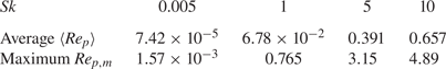
  $3\times 10^5$ (Cliff, Grace & Weber Reference Cliff, Grace and Weber1978). The average and maximum $Re_p$ for the four $Sk$ values considered herein are given in table 1, without exceeding 5.
The average particle Reynolds number  $\langle Re_p \rangle$ and peak value $Re_{p, m}$ for each $Sk$ at time $t^*$ within $X/D=[0.5, 20]$ spanning over all $Y$ and $Z$ directions.
The particle velocity  $\boldsymbol {u}_p$ is advanced forward in time by an adaptive fourth-order Rosenbrock–Wanner scheme with a third-order error estimator and the particle position $\boldsymbol {x}_p$ is temporally updated by an explicit Euler scheme (see Gobert Reference Gobert2010). The particle equations (2.1a,b) are integrated in time with the same time step as used for solving the flow field. The choice of $\tau _f$ used to define $Sk$ can be the nominal time scale $D/U_0$ or the vortex shedding period $T$ or a spanwise-vorticity-based time scale $1/|\omega _z|$. A small $Sk$ indicates that particles maintain a velocity equilibrium with local fluid elements while large- $Sk$ particles are highly self-organized and more loosely coupled to the carrier flow.
2.2. Computational set-up
The MGLET enables a multi-level structured Cartesian mesh (Manhart Reference Manhart2004; Strandenes Reference Strandenes2019) to discretize the computational domain. The overall mesh is generated in a hierarchical structure which consists of multiple cubic grid boxes (grids) at different levels. Each grid is further divided into  $N^3$ uniformly distributed cubic Cartesian cells. A local refinement of the near-cylinder grid is enforced by embedding a zonal algorithm, in which the parental grid is divided into eight equal child grids. A schematic of the multi-level grids at a slice $(Z/D=2.96)$ is shown in figure 1, where five different resolutions are illustrated and the smallest grid cell size is $\varDelta _{min}=0.02D$. A summary of the treatment of the multi-grid hierarchical solution is provided in Appendix A for interested readers. The present spatial resolution is justified to be sufficient for a step cylinder case at a similar $Re$ (Tian et al. Reference Tian, Jiang, Pettersen and Andersson2020), and Jiang et al. (Reference Jiang, Cheng, Draper, An and Tong2016) found that a resolution of 0.05 $D$ utilizing stretching mesh also guarantees a trustworthy transitional wake at $Re=220$. Note that all grids are homogeneous in the spanwise $Z$ direction. The size of the flow configuration is set up as $X/D=[-16.64, 41.6]$, $Y/D=[-8.32, 8.32]$ and $Z/D=[-8.32, 8.32]$, resulting in a total of 71.5 million grid cells. The length of the cylinder span is $L_z\approx 16D$, which is approximately four times the most unstable mode A wavelength $\lambda _z$ according to the mode A wavelength band in numerical work (Henderson Reference Henderson1997) and experimental observation (Williamson Reference Williamson1996). Jiang & Cheng (Reference Jiang and Cheng2017) justified the sufficiency of a spanwise length $L_z>12D$ at $Re=200$ to fully develop typical mode A structures with a large-scale vortex dislocation. A uniform free-stream incoming velocity profile $(U_0, 0,0)$ and a Neumann pressure condition $\partial p/\partial x=0$ are imposed at the inlet plane. At the outlet boundary, we impose Neumann conditions for velocity components $\partial u/\partial x=\partial v/\partial x=\partial w/\partial x=0$ and zero pressure. Free-slip boundary conditions ( $v=0$ and $\partial u/\partial y=\partial w/\partial y=0$) are enforced at the two sidewalls normal to the cross-flow $Y$ direction. An infinitely long cylinder is mimicked by using periodic boundary conditions in the spanwise $Z$ direction. At the surface of the cylinder, no-slip and impermeability boundary conditions are imposed. The boundary condition of particle–wall collisions is defined by a kinetic reduction of both tangential and normal components. The sliding collision model used in the present work is inherited from previous work at $Re=100$ by Shi et al. (Reference Shi, Jiang, Strandenes, Zhao and Andersson2020, Reference Shi, Jiang, Zhao and Andersson2021), where the normal velocity component damps to zero while the tangential component is fully preserved. A peculiar bow-shock clustering induced by the front-end particle–cylinder impaction was reported. The single-phase cylinder wake flow simulation was first run for 400 time units (measured in $D/U_0$) with a time step $0.008D/U_0$ until the flow properly developed into a 3-D state, as visualized in figure 2 by vorticity volume rendering. In the downstream wake, i.e. $X/D = [22, 41.6]$, the primary and secondary vortices might be slightly under-resolved due to lower spatial resolution. In the following, the analysis focuses on the flow and particle fields within the ‘domain of interest’ $X/D = [-2, 22]$ depicted in figure 1 spanning across all the $Y$ and $Z$ directions. Four pairs of streamwise vortices can be clearly observed in the upstream wake. Figure 3(a) shows that the three-dimensionality of mode A wake flow has been well developed after approximately $300 D/U_0$ and the lift coefficient $C_L$ varies periodically onward and with an amplitude lower than in the early stage of the simulation, i.e. before the occurrence of three-dimensionalization. Other flow statistics are sampled from signals within the time window $[300, 400] D/U_0$. The frequency spectra of three velocity components at a sampling point in the centre plane $Y = 0$ are obtained by fast Fourier transform (see figure 3b). The Strouhal number $St = 0.185$ is estimated from the peak frequency of the cross-flow component $f_v$ and the primary vortex shedding period $T$ is thus roughly $5.4 D/U_0$. The vortex shedding period $T$ can be introduced as a physical time scale to define an effective Stokes number, i.e. $Sk_e$. The time-averaged drag coefficient $\langle C_d \rangle$ is estimated as 1.329, which compares well with that reported by Persillon & Braza (Reference Persillon and Braza1998).
 \begin{equation} C_L = 2F_l/\rho_fU^2_0LD, \quad \langle C_d \rangle= \frac{1}{N}\sum_{i=1}^{N}2F_{d,i}/\rho_fU^2_0LD, \end{equation}
where  $N$ is the number of values in the time history of two surface forces within the sampling time interval. Inertial particles are seeded into the 3-D flow with initial velocity $U_0$ at the central part of the inlet plane, as illustrated in figure 1 in a range of $Y/D=[-4.16, 4.16]$. Instead of distributing particles into quiescent regions, i.e. close to the sidewalls, the central part corresponds to the streamwise vortex loops and Kármán vortices possessing major strength. The selective seeding region can reduce the computational dataset. The particle simulation starts at time $t^* = 400D/U_0$ and lasts for $13T$ in order to fully evolve the particles in the 3-D flow field. At each time step, a prescribed number of new particles are injected into the domain while some are leaving through the outlet after about $11T$. Four different Stokes numbers
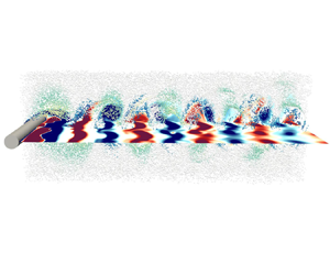
  $Sk = 0.005$, 1, 5, 10 are considered to explore the effects of particle inertia. Figure 4 shows instantaneous particle distributions of the tracer-like ( $Sk = 0.005$) and intermediate ( $Sk = 1$) particles, where the grey particles represent those less affected by the vortex structures in the wake and with only a slight velocity increase, i.e. $|\boldsymbol {u}_p|\in [1,1.1]U_0$. We observe that the almost inertialess particles are fully dispersed throughout the whole domain, while evident void regions are formed by the inertial $Sk = 1$ particles. The accelerated ( $|\boldsymbol {u}_p|>1.1U_0$) and decelerated ( $|\boldsymbol {u}_p|<1U_0$) particles in both cases exhibit an alternating pattern about the centre plane, and the inertial effect is clearly observed in figure 4(b) where the voids indicate a strong influence of the coherent vortices.
Schematic 2-D illustration of the 3-D grid configuration and refinement around the cylinder at  $(X,Y)=(0,0)$ with spanwise vorticity superimposed. The ascending number of levels corresponds to a decreasing spatial resolution $\varDelta$ by a factor of 2. Each square represents a grid box that consists of $N^3$ uniform cubic cells. The ‘volume of interest’ for detailed examinations spans the entire domain in the $Z$ direction with well-resolved large-scale Kármán vortex cells with spanwise vorticity $\omega _zD/U_0 > 1$ and the colour coding shows the alternating sense of spanwise rotation. Particles are injected only over the central half of the inlet plane and subjected to analysis in the indicated ‘domain of interest’.

Volume rendering representation of the instantaneous vorticity field at time  $t^*$, identified by normalized vorticity magnitude $|\omega |D/U_0$ within $[0, 2.3]$. Grey parallel planes illustrate the planes of interest referred to in § 4. Orange and blue swirls with arrows represent positive and negative vortices, respectively, for both the primary spanwise-oriented Kármán cells and the secondary streamwise-oriented braids.

(a) Time history of the lift coefficient  $C_L$ within $[100, 400]D/U_0$, where a regular 3-D state is established in the shaded region. (b) Frequency spectra of the three velocity components $f_{u/v/w}$, where the signals are used to calculate the frequency spectra of three velocity components at the sampling point $(X/D, Y/D, Z/D)=(2, 0, -2.32)$ obtained over $[300, 400]D/U_0$. The Strouhal number $St = 0.185$ representing the primary vortex shedding is obtained from $f_v$, which is half of the peak frequency $f_u$.

Visualizations of instantaneous particle distributions in the domain of interest  $X/D=[-2, 22]$. Side view of inertial particles projected onto the ( $X, Y$) plane: (a) $Sk= 0.005$ and (b) $Sk= 1$. The colour coding represents particle velocity magnitude $|\boldsymbol {u}_p|$ ranging from $0.4U_0$ to $1.3 U_0$.

3. Volume-averaged particle clustering: Voronoï analysis
First, a volume-averaged analysis of the particle concentration based on 3-D Voronoï tessellation is presented in this section. The analysis is confined to the upstream part of the wake in which neither the Kármán rollers nor the braids associated with mode A instability have been subjected to substantial viscous decay. The impact of particle–cylinder collisions, such as the formation of bow-shock clusters (Shi et al. Reference Shi, Jiang, Strandenes, Zhao and Andersson2020), is not evident in the present 3-D wake and can hardly be observed in figure 4. The 2-D Voronoï diagrams do not provide any clear evidence of a dense concentration layer in the vicinity of the cylinder. The effect of front-end particle–cylinder impaction on the particle concentration in the wake region is thus deemed negligible.
3.1. Scales and distributions of Voronoï volumes
We deploy Voronoï diagrams to quantify individual particle clusters, such that a small Voronoï volume is an indicator of locally high particle concentrations, i.e. clustering. The length scale of a certain cluster is an objective measure which only depends on the instantaneous particle distribution. An illustration of the topology of 2-D Voronoï cells in an ( $X,Y$) plane of the particle-laden wake is provided in the snapshot in figure 5. Voronoï cells within the vorticity-dominated wake are clearly larger than the surrounding Voronoï cells. The larger Voronoï cells in the central wake are associated with particularly high fluid vorticity. The evident intensity of local streamwise vorticity observed in figure 5(b) implies a perceptible role of streamwise vortices in particle clustering, besides the prospective effect of Kármán rollers.
A typical 2-D Voronoï cell diagram for  $Sk=1$ particles. The plots show an instantaneous side view of the particle concentration in a thin slice $(Z/D=2.96 \pm 0.1)$ indicated in figure 2. Blue dots represent the individual particle positions and black lines are the borders of each Voronoï cell. The cells are coloured by local (a) spanwise vorticity $\omega _{z, f@p}$ and (b) streamwise vorticity $\omega _{x, f@p}$.

Similarly, Voronoï volumes, i.e. 3-D polyhedral Voronoï cells, are expected to identify and measure clusters and void areas. The quality of the Voronoï analysis and the possibility of identifying a wide range of scales of the particle concentration field depend on the number of sampling particles ( $N_p$). The subsequent analysis considers about $1.9\times 10^5$ particles for each $Sk$ within the truncated domain $X/D = [1, 22]$ spanning over the whole cross-section. The uneven distribution of inertial particles in the near wake is explored by means of the kernel density estimation (k.d.e.) of the Voronoï volumes $\mathcal {V}$ (normalized by the mean value $\langle \mathcal {V} \rangle$). The k.d.e. distribution of the tracer-like $(Sk = 0.005)$ particles in figure 6(a) exhibits a close fit to the two-parameter $\varGamma$ distribution $f(x; a, b)=b^a/\varGamma (\textit {a})x^{a-1}\, {\rm e}^{-x/b}$ with $a = 5$ and $b = 0.2$, as suggested by Ferenc & Néda (Reference Ferenc and Néda2007). The modest deviations from the tails of the $\varGamma$ distribution reflect somewhat higher expectations of smaller and larger Voronoï volumes than in a perfectly random distribution.
Volume-averaged particle statistics for Stokes numbers  $Sk=0.005, 1, 5, 10$. (a) The k.d.e. of normalized Voronoï volumes $\mathcal {V}/\langle \mathcal {V} \rangle$. Here $P_{\mathcal {V}c0}$ and $P_{\mathcal {V}v0}$ denote the intersection points of the k.d.e.s with dotted random $\varGamma$ distribution. These intersection points define the thresholds $\mathcal {V}_{c0}\approx 0.7$ for clusters and $\mathcal {V}_{c0}\approx 2.5$ for voids. The inset compares the mean and standard deviation (std) of the four particle classes. (b) Density distribution of $\mathcal {V}/\langle \mathcal {V} \rangle$. The inset shows the fraction of particles classified as either clusters ( $N_{c0}/N_p$), middle ( $N_{m0}/N_p$) or voids ( $N_{v0}/N_p$).

The normalized k.d.e. distributions intersect the  $\varGamma$ distribution at $P_{\mathcal {V}c0}$ and $P_{\mathcal {V}v0}$, which correspond to normalized Voronoï volumes $\mathcal {V}_{c0}$ and $\mathcal {V}_{v0}$, respectively. Following Monchaux, Bourgoin & Cartellier (Reference Monchaux, Bourgoin and Cartellier2010), Tagawa et al. (Reference Tagawa, Mercado, Prakash, Calzavarini, Sun and Lohse2012), Baker et al. (Reference Baker, Frankel, Mani and Coletti2017) and Momenifar & Bragg (Reference Momenifar and Bragg2020), these intersection points are used to define clusters and voids. The coincidence of intersections for all considered Stokes numbers is consistent with the observation in HIT (Tagawa et al. Reference Tagawa, Mercado, Prakash, Calzavarini, Sun and Lohse2012). In the present particle-laden wake flow, clusters correspond to normalized Voronoï volumes smaller than $\mathcal {V}_{c0}\approx 0.7$ whereas voids are characterized by Voronoï volumes larger than $\mathcal {V}_{v0}\approx 2.5$. It is also noteworthy that all k.d.e.s for $Sk\leqslant 1$ tend to follow a power-law variation with slope $k=-2$ in the void range. This behaviour was also observed in HIT by Monchaux et al. (Reference Monchaux, Bourgoin and Cartellier2010) and Baker et al. (Reference Baker, Frankel, Mani and Coletti2017) and suggests self-similarity of the density distribution of the voids. The probability of clustering is substantially larger for inertial particles than for the tracer-like spheres and the range of the different sizes of Voronoï volumes is much broader, especially for voids, i.e. $\mathcal {V}/\langle \mathcal {V} \rangle$ larger than $\mathcal {V}_{v0}\approx 2.5$. The inset in figure 6(a) shows that the standard deviation and the mean value of the Voronoï volumes also exhibit a non-monotonic variation in $Sk$ with maxima at $Sk=5$. A non-monotonic dependence on inertia of particle clustering in HIT has been reported by Tagawa et al. (Reference Tagawa, Mercado, Prakash, Calzavarini, Sun and Lohse2012) and Baker et al. (Reference Baker, Frankel, Mani and Coletti2017). A possible explanation is that the largest voids observed in the k.d.e. for $Sk=5$ results in the larger standard deviation of $\mathcal {V}/\langle \mathcal {V} \rangle$. The recent work by Momenifar & Bragg (Reference Momenifar and Bragg2020) suggested that the standard deviation of Voronoï volumes is dominant by voids rather than small clusters. This may imply that the standard deviation of the Voronoï volumes cannot in general be considered as an objective indicator to measure the clustering level. A particularly important observation is that the highest occurrence probability of clustering is seen for $Sk = 5$ particles. This particular $Sk$ value well above unity reflects that the nominal Stokes number based on the time scale $D/U_0$ is physically irrelevant in the wake.
The method of defining two thresholds by the intersections between the k.d.e. and  $\varGamma$ distribution is widely applied to estimate the scales of clusters and voids. However, one may question its objectivity since the thresholds are not based on any physical quantities but only on the topology of k.d.e.s. Figure 6(b) shows the density distribution of the four particle classes and the inset shows the fraction of particles in the cluster, void and neutral ranges. The peaks of the distributions for inertial particles are all located to the left of $\mathcal {V}_{c0}\approx 0.7$, while only the tracer-like particles are almost symmetrically distributed about $\mathcal {V}_{c0}$, although slightly skewed to the right. The two thresholds $\mathcal {V}_{c0}$ and $\mathcal {V}_{v0}$ seem most appropriate for the tracer-like $Sk = 0.005$ particles which rarely sample tiny clusters and large voids. The inset shows a decreasing fraction of particle numbers as the scale increases, which is perceptually inconsistent with the density distribution. This can be compared and explained later in figure 9(b).
3.2. Local flow field effects on Voronoï volumes
The effects of particle inertia on the size distribution of Voronoï volumes in figure 6 give an overview of the scale range of particle clustering in the wake. To obtain insight into the likely clustering mechanisms, we now proceed to consider how the size of the individual Voronoï volumes correlates with some local and potentially relevant flow characteristics.
A commonly used method of vortex identification is the  $Q$ criterion (Hunt, Wray & Moin Reference Hunt, Wray and Moin1988). In figure 7, joint distributions of normalized Voronoï volumes versus $Q$ conditioned on particle position ( $Q_{f@p}$) display distinct effects of particle inertia, regarding both the asymmetry about $Q_{f@p}=0$ and the range of $\mathcal {V}$. For the $Sk=0.005$ particles shown in figure 7(a), the normalized Voronoï volumes concentrate within $[0.1, 4]$ and the local $Q$ ranges within $[-2, 2]$, which results in a flat rhomboid shape. These tracer-like particles are almost symmetrically distributed about $Q_{f@p}=0$, thereby indicating a well-mixed process with particles residing in both strain- and rotation-dominant regions. According to the thresholds $\mathcal {V}_{c0}\approx 0.7$ and $\mathcal {V}_{c0}\approx 2.5$, voids are almost non-existent and the particle clustering is modest.
Joint distributions of normalized Voronoï volumes  $\mathcal {V}/\langle \mathcal {V} \rangle$ versus local $Q_{f@p}$ coloured by $R_{Q\mathcal {V}}=\langle \mathcal {V} \rangle Q_{f@p}/\mathcal {V}$. Here $Q_{f@p}$ denotes the value of the normalized $Q$, i.e. $Q(D/U_0)^2$, evaluated at the particle position. Stokes number (a) $Sk=0.005$, (b) $Sk=1$ and (c) $Sk=10$. Dashed greenish curves denote the increasing joint probability density distribution towards centreline $Q_{f@p}=0$.

The joint distributions in figure 7(b,c) show that the  $Q_{f@p}$ range has narrowed to $[-0.5, 0.5]$ while the range of the size of the Voronoï volumes has extended as compared with the data in figure 7(a). This indicates that voids arise and particles cluster more densely in the presence of inertia. Moreover, the joint distributions become highly asymmetric since only a small number of particles sample the rotation-rate-dominant wing with $Q_{f@p}>0$. This asymmetry is particularly evident for $Sk=1$ particles, suggesting that the centrifugal ejection mechanism is even more influential at $Sk$ of unity than for higher $Sk$. The distinct variations of the Voronoï volumes appear mostly at small scales for higher-inertia particles. A number of $Sk=10$ particles appear on the right wing ( $Q_{f@p}>0$) in figure 7(c), which is consistent with the slightly narrower $\mathcal {V}$ range and lower k.d.e. in figure 6(a). The non-monotonic variation with $Sk$ is reflected in both the k.d.e.s and the joint distributions in figure 7. The concentration measure $\mathcal {V}^{-1}$ is most strongly correlated with $Q_{f@p}$ in the clustering range below $\mathcal {V}_{c0}\approx 0.7$. Another scalar field conditioned on particle position, i.e. local vorticity magnitude $|\boldsymbol {\omega }_{f@p}|$, represents the vorticity strength which is equivalent to the square root of the local enstrophy. Figure 8 compares the covariation of the Voronoï volume and $|\boldsymbol {\omega }_{f@p}|$ for each $Sk$. As $Sk$ increases from 0.005 to 1, the size of the Voronoï volumes scale up by two orders of magnitude while the maximum vorticity magnitude of the vast majority of samples reduces dramatically. At $Sk=10$, however, more particles are located in higher- $|\omega _{f@p}|$ regions while the range of $\mathcal {V}$ slightly narrows. We observed in figure 2 that the large- $|\boldsymbol {\omega }_{f@p}|$ above $2U_0/D$ are evident in the upstream Kármán vortices and the separated shear layers. The spanwise vorticity intensity in figure 2 decays downstream to around $0.5U_0/D$ at $X/D=22$ while the streamwise component ranges roughly from $0.65U_0/D$ to $0.30 U_0/D$ within $X/D=[8, 22]$. Tracer-like particles can stay within the separated shear layers or be trapped in the recirculation region, as reflected by several exceptionally high $|\boldsymbol {\omega }_{f@p}|$ values in figure 8(a). By contrast, more inertial particles are most often expelled out of the primary vortex core regions and such ejections are most prominent at $Sk=1$. The almost ballistic $Sk=10$ particles, however, can partially penetrate the separated shear layers and the circumference of rotation-dominant regions, as evidenced by relatively large $|\omega _{f@p}|$ values in figure 8(c). Strong correlations between the reciprocal Voronoï volume $\mathcal {V}^{-1}$ and the collocated vorticity magnitude $|\omega _{f@p}|$ are measured by $R_{|\omega |/\mathcal {V}}$ and observed way below $\mathcal {V}_{c0}\approx 0.7$. The joint distributions in figures 7 and 8 reveal how clusters and voids are associated with the local flow quantities. The effect of particle inertia also appears non-monotonically in Stokes number and $Sk=1$ exhibited the strongest inertial effect of the cases considered. These covariances alone do not reflect how the size of the Voronoï volumes is related to either of the correlations $R_{|\omega |/\mathcal {V}}$ and $R_{Q/\mathcal {V}}$. Figure 9(a,c) shows how the Voronoï-bin-averaged correlations $R_{|\omega |/\mathcal {V}}$ and $R_{Q/\mathcal {V}}$ vary with the size of the normalized Voronoï volume. It is observed that both $R_{|\omega |/\mathcal {V}}$ and $R_{Q/\mathcal {V}}$ decrease almost to zero when $\mathcal {V}/\langle \mathcal {V} \rangle$ exceeds 0.2, thereby indicating that the particle clustering is completely decorrelated from the vortex cores. Based on the decaying correlations, we thus propose the stricter threshold $\mathcal {V}_{c1}\approx 0.2$ for clustering. An evident $Sk$ effect is only observed for small Voronoï volumes, i.e. $\mathcal {V}/\langle \mathcal {V} \rangle$ below $\mathcal {V}_{c1}$. The $Sk = 1$ particles are almost consistently distributed below $R_{Q/\mathcal {V}}= 0$ and exhibit the tiniest Voronoï volumes. This is another manifestation of the observation that the $Sk = 1$ particles cluster more densely than the other particle classes considered.
Joint distributions of  $\mathcal {V}/\langle \mathcal {V} \rangle$ versus local vorticity magnitude $|\omega _{f@p}|$ coloured by $R_{|\omega |\mathcal {V}}=\langle \mathcal {V} \rangle |\omega _{f@p}|/\mathcal {V}$ at different Stokes numbers (a) $Sk=0.005$, (b) $Sk=1$ and (c) $Sk=10$.
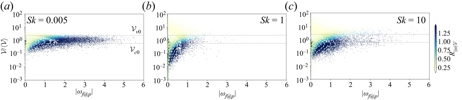
Voronoï-bin averages versus normalized Voronoï volume: (a)  $R_{|\omega |/\mathcal {V}}$; (b) $|\omega _{f@p}|$; (c) $R_{Q/\mathcal {V}}$; (d) $Q_{f@p}$. The data are averaged within narrow segments of the logarithmic Voronoï volume axis [ $10^{-3}, 10^2$] and the mean correlations in (a) and (c) are normalized by the maximum value for each $Sk$. The vertical dashed lines represent new thresholds for clusters and voids, i.e. $\mathcal {V}_{c1}\approx 0.2<\mathcal {V}_{c0}$ and $\mathcal {V}_{v1}\approx 2.5=\mathcal {V}_{v0}$, respectively. The inset in (b) shows the fraction of particles classified as either clusters ( $N_{c1}/N_p$), middle ( $N_{m1}/N_p$) or voids ( $N_{v1}/N_p$) based on the same samples in figure 6(b).
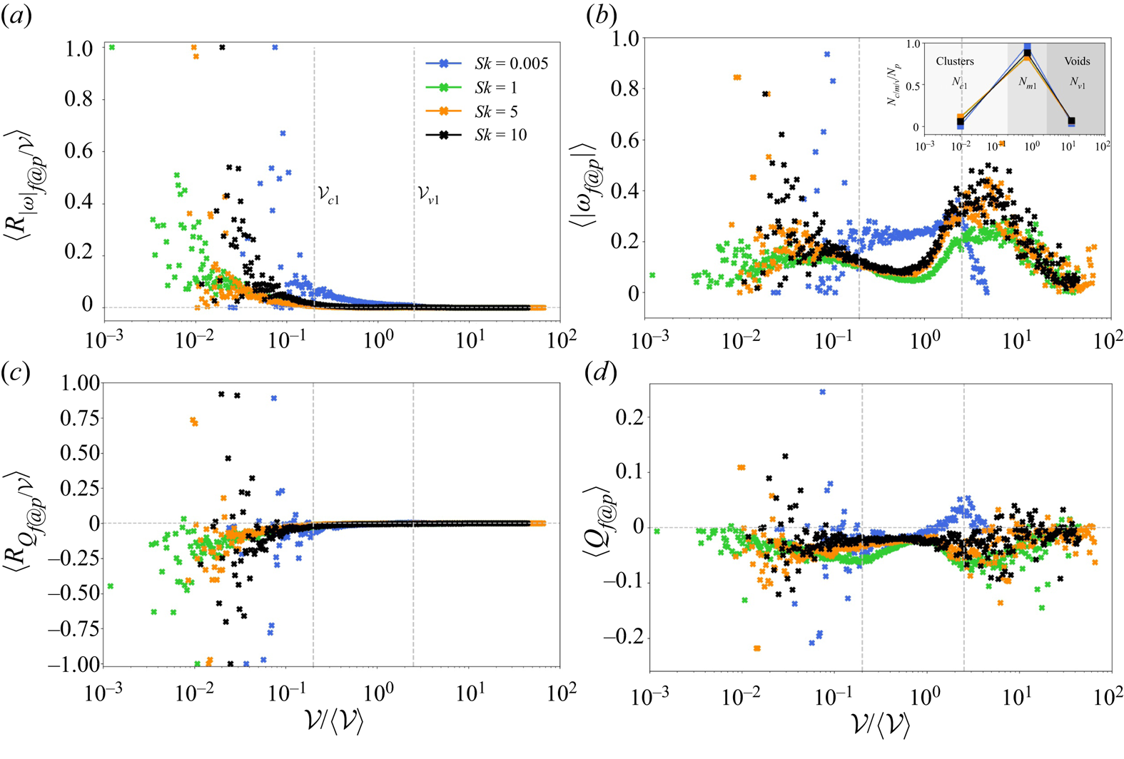
Figures 9(b) and 9(d) show how the Voronoï-bin-averaged local  $|\omega _{f@p}|$ and $Q_{f@p}$ vary with the normalized Voronoï volumes and add more quantitative information than the joint distributions in figures 7 and 8. The bimodal variation of $\langle |\omega _{f@p}| \rangle$ with local peaks at small and large scales is particularly interesting. The data for the inertial particles are fairly close in the middle range from $\approx 0.2$ to 2.5 and yet different from those for the $Sk = 0.005$ particles. The tracer-like particles are limited to $\mathcal {V}/\langle \mathcal {V} \rangle <5$, which reflects a fairly uniform particle distribution. In striking contrast, volumes more than 50 times larger than the average volume $\langle \mathcal {V} \rangle$ can be seen for the inertial particles. Irrespective of Stokes number, however, the conditionally averaged vorticity $|\omega _{f@p}|$ shows a decreasing trend with increasing Voronoï volumes although the decay sets in later for higher $Sk$. We believe that the rightmost peak of the bimodal distributions results from particles partially embedded in the most upstream and thus most energetic Kármán rollers, whereas $|\omega _{f@p}|$ decreases for more downstream voids in cells with gradually decaying vortex strength. A new threshold $\mathcal {V}_{v1}\approx 2.5$ for the existence of void areas can now be based on the bimodal distribution. This happens to be the same as the earlier threshold $\mathcal {V}_{v0}$ based on the k.d.e.s in figure 6.
At small scales of the Voronoï volumes ( $<\mathcal {V}_{c1}$), the spread of the scatters is more evident than at larger scales and rapid variations of $|\omega _{f@p}|$ between nearby $\mathcal {V}$ values are seen. The very large $|\omega _{f@p}|$ is likely corresponding to clusters located either on the cusps of primary vortex-core regions or in the separated shear layers. Rapid changes of both $|\omega _{f@p}|$ and $Q_{f@p}$ are observed for $\mathcal {V}/\langle \mathcal {V} \rangle$ below 0.1, while similar abrupt changes occur only for even smaller Voronoï volumes for $Sk=5$ and 10. By contrast, the variations of $|\omega _{f@p}|$ and $Q_{f@p}$ for $Sk=1$ particles are relatively modest and therefore indicate the least correspondence with vortex-core regions, i.e. maximum void formation and clustering. The extremely high $\langle Q_{f@p} \rangle$ values for $Sk=5$ and 10 particles at cluster scale in figure 9(d) appear in both strain- and rotation-dominant regions, while the corresponding extreme scatters of $\langle |\omega _{f@p}| \rangle$ indicate their appearance in the uppermost wake region. It is therefore most likely that these extremal scatters are associated with the shear-layer regions although the Voronoï volumes further downstream can return multi-valued $\langle |\omega _{f@p}| \rangle$.
As indicated in figure 4, inertial particles experience decelerations and accelerations during their interactions with the transient vortex structures. Figure 10 shows how the velocity distributions of the accelerated (figure 10b,d, f) and decelerated (figure 10a,c,e) particles vary with the scale of Voronoï volumes for the three  $Sk$ cases. The velocity magnitude of the $Sk=0.005$ particles in figure 10(a,b) ranges widely from $0.2U_0$ to $1.4 U_0$. Particles trapped in the recirculation region or approaching the stagnation point decelerate to the lowest whereas those within the vortex cores remain $0.6U_0$– $0.7U_0$, as illustrated in figure 4(a). The majority of the tracer-like particles correspond to Voronoï volumes $\mathcal {V}_{c1}<\mathcal {V}/\langle \mathcal {V} \rangle <\mathcal {V}_{v1}$ with a slight bias towards the cluster scales and well mixed over the $Q$ field. As $Sk$ increases, the number of accelerated particles reduces remarkably while the range of Voronoï volumes extends much wider, notably at $Sk=1$. Also the high- $|\boldsymbol {u}_p|$ particles are mostly located in strain-dominant regions.
Joint distributions of normalized Voronoï volumes  $\mathcal {V}/\langle \mathcal {V} \rangle$ versus particle velocity magnitude $|\boldsymbol {u}_p|$ coloured by $Q_{f@p}$. Particles are filtered by $|Q_{f@p}|>0.2$. Stokes number (a,b) $Sk=0.005$, (c,d) $Sk=1$ and (e, f) $Sk=10$. The horizontal dashed lines are the new thresholds for clusters and voids, i.e. $\mathcal {V}_{c1}\approx 0.2$ and $\mathcal {V}_{v1}\approx 2.5$, defined in figure 9.

By contrast, the lowest  $|\boldsymbol {u}_p|$ of the inertial particles is in the range $[0.55U_0\text {--}0.65 U_0]$. The majority of the decelerated $Sk=1$ particles are concentrated within a medium range of Voronoï volumes, while larger volumes are more frequently observed for $Sk=10$. Unlike the accelerated inertial particles, the decelerated particles are more involved with vortex structures since an increasing number of such particles are observed in rotation-rate-dominant regions as $Sk$ increases. It is exceptional that positive- $Q_{f@p}$ samples are almost negligible for $Sk=1$, which reveals that the particles are subjected to strong centrifugal ejections from the vortices. We also observe that the number of decelerated particles outweighs that of accelerated particles, as visualized earlier in figure 4. Those joint distributions manifest the role of particle inertia, parameterized by $Sk$, in particle acceleration and deceleration. To this point, it is certainly beneficial to include physical significance to define the scales of clusters and voids through the newly proposed thresholds. The inclusion of variations of flow quantities, to a great extent, corrected the bias of pure Voronoï size-based cluster thresholds. However, it should be clarified that these thresholds also hold over a range of applicable situations where particle clustering is preferentially sampled by underlying flow structures. Therefore, the local $Q$- or vorticity-based thresholds outperform the probability-distribution-based ones in such vortical flows. Tom & Bragg (Reference Tom and Bragg2020) discussed the relevant question in the context of particle settling, where clustering still appears at small scales, yet uniformly sampled by the velocity gradient field in the limit of a large gravity force. This observation indicates that the dominance of preferential sampling by the local flow field heavily depends on settling scales. In this scenario, the physics-based identification is confined by the presence of settling, while the conventional probability-density-distribution-based criterion may be more suitable in other scenarios.
4. Planar clustering patterns
The effect of particle inertia on clustering is thoroughly investigated by means of joint distributions of local flow characteristics and Voronoï voulmes in § 3. However, the 3-D Voronoï analysis does not enable us to distinguish the separate effects caused by the spanwise-oriented Kármán rollers and the streamwise-oriented braids resulting from mode A instabilities. We therefore proceed to analyse how the in-plane clustering varies in different directions with the intention of demonstrating the different roles of the primary and secondary vortices in the local clustering patterns and particle dynamics.
4.1. Secondary clustering and continuous voids
Figure 11(a–d) shows the topology of the  $Q$ field of the particle distribution in an ( $X, Y$) plane for $Sk=1$. Figure 11(a,b) presents the results at a spanwise location midway between two counter-rotating streamwise vortices, so that the flow field is almost 2-D and resembles the purely 2-D flow at $Re = 100$, i.e. well below the onset of mode A instability. In figure 11(e, f), the $Q$ field from the 2-D wake at $Re = 100$ exhibits the dominant Kármán rollers and qualitatively resembles the spanwise vortices in figure 11(a,b), despite some slight topological differences. It is therefore not surprising to learn from figure 11( f) that the topology of the particle clustering also resembles the concentration patterns reported by Shi et al. (Reference Shi, Jiang, Zhao and Andersson2021).
Planar  $Q$ field (a,c,e) in a specific ( $X,Y$) plane and particle distribution in a 0.2 $D$ thick slice about that $Z$ (b,d, f) for $Sk = 1$ particles for the present case $Re=200$: (a,b) $Z/D = 2.0$; (c,d) $Z/D = 2.96$. The particles are coloured by $|\boldsymbol {u}_p|$. The same colour bars are used at both locations and the two slices are shown in figure 2. (e, f) In comparison with (a,b), the $Q$ field and particle distribution at $Re=100$ flow without the three-dimensionalization are presented (Shi et al. Reference Shi, Jiang, Zhao and Andersson2021).

A more interesting observation in figure 11(c,d) shows the vortex and concentration fields at a spanwise interval 0.96 $D$, i.e. about 1/4 of $\lambda _z$ of mode A instability, away from the plane in figure 11(a,b). The spanwise position $Z/D = 2.96$ is the same as that considered in figure 5, where the vorticity contours show the presence of significant streamwise vorticity along with the usual spanwise vorticity. The $Q$ field in figure 11(c,d) confirms the presence of strong vortical flow in the braid areas (left) which gives rise to secondary void areas (right), which is considered as a result of inertial particles being expelled from the streamwise vortical loops. The outcome is the formation of an almost continuous void passage which persists at least 20 $D$ downstream. Another important observation is that particles trapped between Kármán cells and streamwise vortices form an inner layer of densely concentrated particles. Such inner clusters are seen neither in the plane 0.96 $D$ apart nor in the 2-D wake at $Re = 100$ (Shi et al. Reference Shi, Jiang, Zhao and Andersson2021). The formation of inner clusters is clearly an effect of the presence of streamwise vortices at $Re = 200$. This strongly suggests that the particle clustering is likely to exhibit substantial variations in the spanwise direction. Figure 12 shows the variation of slice-averaged particle velocity magnitude $|\boldsymbol {u}_p|$. The cyan and red squares plotted along the dashed line $|\boldsymbol {u}_p|=1U_0$ represent the positions of the cores of and the midpoints between streamwise vortices, respectively. These positions are identified by visual inspections of isocontours of the vorticity field. The presence of eight cyan squares, about 2.07 $D$ apart, implies that the flow field comprises four pairs of counter-rotating streamwise vortices. This is consistent with the chosen width $L_z = 16.64D$ of the computational domain, which leaves room for 4 wavelengths $\lambda _z$ of mode A instability. In contrast, the spanwise width $L_z = 10D$ used by Luo et al. (Reference Luo, Fan, Li and Cen2009) does not match with an integer multiple of $\lambda _z\approx 4D$. In view of the goal of the present study, namely to explore the consequences of the occurrence of the streamwise-oriented vortex braids on the particle concentration, we refrain from averaging the particle distribution in the inhomogeneous spanwise direction.
Spanwise variation of particle velocity magnitude  $|\boldsymbol {u}_p|$ averaged over individual ( $X,Y$) planes for $Sk = 0.005$, 1, 5, 10. Cyan squares denote the approximate $Z$ positions of streamwise vortex cores while red squares denote $Z$ positions midway between two neighbouring streamwise loops.

The particle velocity  $|\boldsymbol {u}_p|$ appears quasi-periodic in the spanwise direction with a local minimum near the position of the cyan squares, thereby suggesting an attenuation of the particle velocity by the streamwise vortices. Near the position of the red squares, where the mode-A-induced vortices are of negligible influence, $|\boldsymbol {u}_p|$ attains local maxima. This peculiar periodicity can be observed for all the four particle classes, although the actual particle velocity is higher for $Sk = 1$ particles than both for the tracer-like particles as well as for more inertial particles. Once again we observe that $Sk = 1$ particles exhibit the strongest effect of inertia. Although the data in figure 12 have been averaged both in $X$ and $Y$ as well as over the slice thickness ${\rm \Delta} Z$, the slice-averaged particle velocity exceeds the inlet velocity $1U_0$ over almost the entire span. This can only be explained by the centrifugal mechanism which expels inertial particles out of the vortical structures and therefore also away from the core of the wake where a substantial velocity defect is present in the fluid flow field.
4.2. Ribbon clumps
Large-scale vorticial flow structures are influential mostly within  $Y/D=[-3, 3]$ in the cross-flow direction (see figure 2). Let us therefore take a close look at the flow field (figure 13a–c) and particle concentration (figure 13d–f) in three representative horizontal planes. At the centre plane of the wake, shown in figure 13(a), we observe that the primary Kármán vortex cells are disrupted, apparently by the presence of streamwise braid vortices. This plot is encouragingly similar to the flow visualization shown by Williamson (Reference Williamson1996) in his figure 13(a). His experiments were also at $Re = 200$ and the spanwise wavelength reported $\lambda _z = 4.01D$. The primary Kármán vortices are deformed in a wavy fashion along their length, which results in local formation of vortex loops with a spanwise length scale around 3 to 4 diameters (Williamson Reference Williamson1996). In contrast, particles cluster in ribbons aligned with the cylinder axis in the space between two consecutive spanwise vortices. Shortly downstream of the cylinder, however, discrete clumps of particles appear along the otherwise thin ribbons. The four clumps, about 4 $D$ apart, observed in figure 13(d) correspond with the four vortex loops (red) seen in figure 13(a). The large amount of particles aggregate into clumps because of the sweeping motion of two neighbouring counter-rotating spanwise vortex cells. The particle ribbons can therefore persist only in regions where the Kármán rollers are uninterrupted by the presence of streamwise braids. The clumps are most pronounced at $X/D=[5, 7]$ and gradually shrink further downstream while the ribbons in between become wavy. The self-similarity of this peculiar clustering pattern persists beyond $X/D = 20$. However, the particle pattern in figure 13(a,d) is qualitatively different from that shown in figure 6(b) of Luo et al. (Reference Luo, Fan, Li and Cen2009). Despite the $Sk$ being the same, the higher Reynolds number $Re = 260$ makes their flow field more complex, probably with coexistence of mode A and mode B instabilities. On approaching the sidewalls, for instance at $Y/D = 1$ and 2 (see figures 13b,e and 13c, f, respectively), only the upper side of the vortex street is felt and the streamwise distance between neighbouring vortex structures is therefore doubled compared to at the midplane. Nevertheless, the ribbon-clump clustering is retained also at $Y/D = 1$ and even the streamwise periodicity remains the same as at $Y/D = 0$. This is apparently a memory effect due to particle inertia. The particles are also more dispersed and start to invade the originally void areas between two consecutive ribbon-clump clusters, especially around $Z/D = 2$ where a vortex dislocation occurs. It is interesting to see the close resemblance with the experimental flow visualization in figure 8 in Zhang et al. (Reference Zhang, Fey, Noack, König and Eckelmann1995) at $Re = 196$ by means of hydrogen bubbles released from a wire located at $(X/D, Y/D) = (2, 1)$. It is evident that the streamwise vortices play a major role in the particle clustering in the $(X, Z)$-plane off-set 2 $D$ from the midplane. Figure 13(c, f) shows that the ribbon-clump pattern has been dispersed, although a spanwise periodicity with wavelength of approximately 4 $D$ still persists, at least for $X/D > 10$ where four partially empty void circles can be seen.
Planar  $Q$ field (a–c) in a specific $(X,Z)$ plane and particle distribution in a 0.2 $D$ thick slice about that $Y$ (d–f) for $Sk = 1$ particles. The particles are coloured by $|\boldsymbol {u}_p|$. Positions (a,d) $Y/D = 0$, (b,e) $Y/D = 1$ and (c, f) $Y/D = 2$. The same colour bars are used for all locations.

The slice-averaged particle velocity over thin  ${\rm \Delta} Y$ slices is shown in figure 14(a). The symmetric velocity variation for tracer-like $Sk = 0.005$ particles resembles the well-known variation of the streamwise fluid velocity across the wake. The maximum velocity defect at $Y = 0$ is about $0.2U_0$, while the ‘free-stream’ particle velocity is 4 % above $U_0$. The particle velocity defect is almost halved for the $Sk = 1$ particles, and somewhere between $0.1 U_0$ and $0.2 U_0$ for the most inertial particles. Figure 14(b) shows the variation of the volume-averaged local spanwise vorticity $\langle \omega _{f@p,z} \rangle$, where an almost perfect antisymmetric distribution is observed for the tracer-like $Sk = 0.005$ particles, just as for the variation of the Eulerian fluid vorticity $-\partial U/\partial Y$ across the wake. The peak positions of $\langle \omega _{f@p,z} \rangle$ are dependent on particle inertia and are furthest away from the midplane of the wake for $Sk = 1$ particles, for which the peak values also are most noticeably decreased. The substantial reduction of the fluid vorticity $\langle \omega _{f@p,z} \rangle$ seen by the inertial particles indicates that these particles are expelled from the cores of the Kármán vortex cells, whereas the tracer-like particles populate the entire flow field. Since the fluid vorticity conditioned on particle position is a subset of the Eulerian vorticity field, the substantial reduction of $\langle \omega _{f@p,z} \rangle$ for $Sk \geq 1$ indicates an indirect effect of particle inertia. It is noteworthy that the particle velocity for $Sk = 0.005$ and $Sk = 1$ particles almost coincides outside of the wake region, i.e. for $| Y/D | > 1.5$, whereas $|\boldsymbol {u}_p|$ is lower for the more inertial particles. This is in striking contrast with the $Sk$ dependence of the particle velocity at themidplane where the tracer-like particles behave very differently from the $Sk = 1$ particles. This observation can probably be explained by the introduction of an effective Stokes number, i.e. $Sk_e=\tau _p/\tau _{fe}$, based on a physically relevant time scale $\tau _{fe}$ of the local flow field. The time scale $\tau _f=D/U_0$ originally used to define the nominal $Sk$ serves well only for book-keeping purposes. A time scale based on the primary shedding frequency in figure 3(b) will be more relevant but cannot reflect any spatial variations of the carrier flow. We therefore choose a spanwise-vorticity-based fluid time scale, i.e. $\tau _{fe}=1/|\omega _{z}|$, to account for variations of the flow field in both the cross-flow and the streamwise directions. The $Sk = 1$ particles behave clearly as inertial around the midplane of the wake where the fluid vorticity is largest due to the dominant influence of the vortical Kármán cells which make the local fluid time scale $\tau _{fe}$ small and the effective Stokes number $Sk_e=\tau _p|\omega _{z}|$ large. The vorticity-based time scale $\tau _{fe}=1/|\omega _{z}|$ increases rapidly with the distance $Y$ from the midplane (see figure 14b) and gives rise to a substantial reduction of $Sk_e$ such that the $Sk = 1$ particles experience a receding effect of inertia in the outer parts of the wake. The $Sk = 5$ and 10 particles are sufficiently inertial to still behave inertially in the outskirts of the wake.
(a) Slice-averaged particle velocity magnitude  $|\boldsymbol {u}_p|$ and (b) spanwise vorticity conditioned on particle positions $\langle \omega _{f@p,z} \rangle$ for four different $Sk$ numbers, together with the unconditioned spanwise vorticity $\langle \omega _{f,z} \rangle$ (grey curve denoted $Sk=0$).

4.3. Cross-sectional clustering patterns and tubular voids
Clustering of  $Sk = 1$ particles in two cross-sectional planes is presented in figure 15. The two planes at $X/D = 11.5$ and 13.5 shown in figure 2 cut through the centres of two consecutive Kármán vortices and the actual distance 2 $D$ between the planes is $\approx 0.5\lambda _x$. Despite the disruption of the Kármán vortices by streamwise-oriented secondary vortices observed in figure 13(a) and in figure 15(c), a non-interrupted void area is observed in figure 15(a,b). This continuous void extends all along the spanwise with a thickness larger than 2 $D$. The red circular contours at $Y/D \approx \pm 2$ in the $Q$ field signify the streamwise-oriented braid vortices and give rise to circular void areas in figure 15(a,b). These void areas, some of which are indicated in black, are cuts through tubular void cells.
Cross-sectional distribution of  $Sk = 1$ particles coloured by particle velocity magnitude $|\boldsymbol {u}_p|$ (a,b) and the corresponding planar $Q$ field (c,d) at (a,c) $X/D \approx 11.5$ and (b,d) $X/D \approx 13.5$. The black dotted circles in the upper panels show tubular voids.

The clustering patterns in figure 15(a,b) are very similar. However, a closer look shows that the particle clustering just above the continuous void in figure 15(a) and the particles below the spanwise void in figure 15(b) have a higher speed than the other particles. This phenomenon cannot be ascribed to the streamwise-oriented vortices, which always appear in oppositely rotating pairs. The Kármán cell at  $X/D = 11.5$ has negative $\omega _z$ while $\omega _z$ is positive at $X/D = 13.5$ (see figure 5a). The fluid velocity component in the streamwise direction is therefore locally high above the vortex centre at $X/D = 11.5$ and below the vortex centre at $X/D = 13.5$. This explains why the particle velocities in figure 15(b) are upside-down compared with those in figure 15(a).
The streamwise variation of the slice-averaged particle velocity  $\langle |\boldsymbol {u}_p| \rangle$ is shown in figure 16(a). The particle velocity varies periodically with wavelength $\approx 2D\approx 0.5\lambda _x$ since individual vortex cells contribute equally to the volume-averaged velocity irrespective of its sense of rotation. The minima of $\langle |\boldsymbol {u}_p| \rangle$ for the tracer-like particles correspond to the cores of the Kármán cells (cyan squares) and the maxima are about midway (red squares) between two consecutive vortex cells. Also, the spanwise vorticity $\langle \omega _{f@p,z} \rangle$ varies periodically in figure 16(b), but with a wavelength $\approx 4D \approx \lambda _x$, i.e. twice the periodicity found for $\langle |\boldsymbol {u}_p| \rangle$. The spatial periodicity reflects the vortex shedding process frozen at one time step. The cyan squares match well with the peaks and troughs of the spanwise vorticity, thereby reflecting the alternating sense of rotation in consecutive cells. The midpoints (red squares) correspond well with the locations where $\langle \omega _{f@p,z} \rangle$ changes sign. The most inertial particles ( $Sk = 5$ and 10) show similar periodic variations. Despite the phase shift, the wavelengths of the periodicity at $Sk = 5$ and 10 are the same as those for $Sk = 0.005$. However, the amplitude of the spanwise vorticity variations has been reduced, apparently since these inertial particles are expelled from the Kármán cells by the centrifugal mechanism. It is noteworthy that the $Sk = 1$ particles behave differently and their behaviour does not strongly correlate with the Kármán vortex street, which is another manifestation of the strongest inertial effect at $Sk = 1$. The majority of these particles are preferentially concentrated outside of the vortical flow structures, as reflected by the very modest spanwise vorticity at the particle positions shown in figure 16(b). In other words, the $Sk = 1$ particles reside primarily in strain-dominant regions, contrary to the tracer-like $Sk = 0.005$ particles which are almost homogeneously distributed and accordingly populate even the vortex cores. Despite the fairly periodic variations of $|\boldsymbol {u}_p|$ and $\langle \omega _{f@p, z} \rangle$ in figure 16(a,b), the particle velocity as well as the peaks of the fluid vorticity are decaying in the streamwise direction. This trend is particularly clear for the tracer-like particles, which are supposed to be the only ones that closely reflect the streamwise decay of the Kármán vortex cells. The behaviour of the sampled vorticity field by the more inertial particles is different. The vorticity amplitude for the $Sk = 5$ particles does exhibit a decaying trend and the vorticity amplitude sampled by the $Sk = 10$ particles is even increasing with streamwise distance. This is obviously an indirect effect of particle inertia at different $Sk$ as particles are convected downstream with the shed vortices. The heaviest particles behave more ballistically and are therefore able to partly penetrate the vortex cells and sample the high-vorticity field therein.
Streamwise variation of (a) particle velocity magnitude  $|\boldsymbol {u}_p|$ and (b) slice-averaged spanwise vorticity $\langle \omega _{f@p, z} \rangle$ averaged over individual ( $Y,Z$) planes for $Sk = 0.005$, 1, 5, 10. Cyan squares denote the approximate $X$ positions of the cores of Kármán vortex cells while red squares denote $X$ positions midway between two consecutive Kármán cells.

We have learned from the results shown in this section that the clustering patterns are influenced not only by the spanwise vortices, as at  $Re = 100$, but also by the streamwise vortices which emerge as a result of mode A instabilities. We observed varying clustering patterns in both horizontal and cross-sectional planes. The variations of slice-averaged particle velocity $|\boldsymbol {u}_p|$ reflect the streamwise periodicity of the spanwise-oriented vortex cells and the spanwise periodicity of the streamwise vortices. Generally, the local vortex structures tend to reduce the particle velocity magnitude for $Sk > 1$ inertial particles. All planar observations in this section support the conclusion from the preceding § 3 that the strongest effects of inertia occur for $Sk = 1$ particles.
5. Concluding remarks
In the present work, we have employed one-way coupled Eulerian–Lagrangian simulations of particle-laden flow to investigate the preferential concentration of inertial point particles in the 3-D laminar wake of a circular cylinder at  $Re=200$. The mode A instability in this transition regime induces streamwise vortices separated about 4 $D$ in the spanwise direction, which are likely to influence the particle dynamics and the topology of the particle clustering. Despite being unsteady and 3-D, the vortical flow field in the near wake is particularly attractive to in-depth explorations of how particles organize themselves in a wake with secondary vortex loops coexisting with the large-scale Kármán rollers.
Volume-averaged Voronoï analysis has been used to explore how the size of clusters and voids depends on particle inertia characterized by Stokes number ( $Sk$). The formation of the voids and clusters is believed to result mainly from the centrifugal ejections by local coherent vortices. In agreement with the observation in HIT (Monchaux et al. Reference Monchaux, Bourgoin and Cartellier2010; Tagawa et al. Reference Tagawa, Mercado, Prakash, Calzavarini, Sun and Lohse2012; Baker et al. Reference Baker, Frankel, Mani and Coletti2017), the inertia effect reflected by the probability distributions of Voronoï volumes was more pronounced at the cluster scale than at the void scale, the latter exhibiting self-similarity. While Monchaux et al. (Reference Monchaux, Bourgoin and Cartellier2010) proposed probability-distribution-based thresholds for clusters and voids, we instead suggested a physics-based identification criterion. The correlations between the Voronoï volume and either of the conditioned scalar fields of $Q_{f@p}$ and $|\omega _{f@p}|$ almost decay to zero at $\mathcal {V}/\langle \mathcal {V} \rangle \approx 0.2$, thereby suggesting strong clustering. This represents a major distinction from the conventional threshold $\mathcal {V}/\langle \mathcal {V} \rangle \approx 0.7$ given by the intersection point of the $\varGamma$ distribution and k.d.e.s of Voronoï volumes. The divergence at large Voronoï scales in the bimodal variations of $Q_{f@p}$ and $|\omega _{f@p}|$ indicated voids at $\mathcal {V}/\langle \mathcal {V} \rangle \approx 2.5$, which is very close to the threshold measured from the k.d.e.s. These new thresholds were also more consistent with the sparse sample density at the tails of the distributions. Particles’ preferential sampling of high-strain/low-vorticity regions was demonstrated by the joint distributions of Voronoï volumes $\mathcal {V}$ and $Q_{f@p}$, whereas the role of the centrifugal mechanism in the separated shear layers and in the immediate vicinity of the cylinder showed up in $\mathcal {V}$– $|\omega _{f@p}|$ scatter plots. Particularly strong clustering was observed at $Sk=1$ and a non-monotonic $Sk$ dependence was found in both joint distributions. This finding contrasts with the monotonic $Sk$ trend seen in the dispersion function by Yao et al. (Reference Yao, Zhao, Hu, Fan and Cen2009) in the 2-D wake at $Re=100$. However, the present results are in accordance with the non-monotonic $Sk$ dependence of the spanwise dispersion function reported by Luo et al. (Reference Luo, Fan, Li and Cen2009) in a 3-D wake at $Re=260$, even though mode B and mode A instabilities are coexisting at that $Re$.
$Re$.
The instantaneous distributions of particle velocities and positions revealed areas with distinct particle acceleration and deceleration, which we ascribed to particle inertia either aiding or opposing the local vortex structures. With increasing  $Sk$, the acceleration of inertial particles diminished, while the velocity distribution of the decelerated particles was only modestly affected. The $Sk=1$ particles were least coupled to the vortical motions since the majority of decelerated particles were expelled from vorticity-dominant regions.
In addition to the volume-averaged Voronoï analysis, planar distributions showed that clusters and voids in the  $(X,Y)$ plane were formed by the Kármán rollers, similarly to that in the 2-D wake at $Re=100$ (Yao et al. Reference Yao, Zhao, Hu, Fan and Cen2009; Shi et al. Reference Shi, Jiang, Zhao and Andersson2021). In addition, however, the secondary vortices give rise to inner clusters with a spanwise periodicity associated with mode A instability, which were non-existent at $Re=100$ (Yao et al. Reference Yao, Zhao, Hu, Fan and Cen2009; Shi et al. Reference Shi, Jiang, Zhao and Andersson2021). Clusters and voids caused by the secondary streamwise-oriented braids were observed also in the cross-sectional plane. The averaged particle velocity magnitude exhibited spatial periodicities associated with the Kármán cells in the streamwise direction and the streamwise vortex loops in the spanwise directions. Local minima of $\langle |\boldsymbol {u}_p| \rangle$ were ascribed to these braids and observed $\approx 0.5\lambda _z\approx 2 D$ apart along the span. Also these effects were most pronounced at $Sk=1$.
Another manifestation of the streamwise braids was the discrete particle clumps, about  $4D$ apart, on the otherwise thin ribbon-like clusters formed between two consecutive Kármán rollers. Particles aggregated in such clumps because the inertial particles were first centrifuged out of the vortical braids and subsequently swept towards the centre plane, cf. figure 13(a), by two neighbouring counter-rotating streamwise vortices.
The presence of streamwise-oriented vortices at  $Re = 200$ induces a more complex clustering and void topology than in the 2-D wake at $Re = 100$. The secondary vortex braids had a surprisingly strong influence on the particle distributions in the near wake. The highly non-uniform distribution of particles in the spanwise direction may have practical consequences in applications where even distributions are desired.
Funding
Computational resources were provided by Norwegian HPC infrastructure (www.sigma2.no), under project nn2649k granted by the Norwegian Research Council. This work is financially supported by NTNU Energy through a research fellowship. L.Z. acknowledges the Natural Science Foundation of China (grant nos 11911530141 and 91752205).
Declaration of interests
The authors report no conflict of interest.
Appendix A. Algorithm of multi-level grid solution
In § 2.2, the cross-sectional hierarchical structure of the multi-level grid is depicted in figure 1. The overall mesh is generated from coarse to fine grid cells while the solutions for pressure and velocities are transferred from fine to coarse grid cells in the overlapped regions. A summary of the algorithm regarding the multi-level grid solution is given as follows.
(1) Divergence field.
Before updating the pressure and velocity field at the new time step $n+1$, the intermediate velocity field $\boldsymbol {u}^*$ is computed with the evaluated viscous, convective and pressure gradient terms in Navier–Stokes equations as input at previous time steps, given as
(A 1)The divergence field is thus computed from\begin{equation} \boldsymbol{u}^*=\boldsymbol{u}^{n-1}+2{\rm \Delta} t\left[(\boldsymbol{u}^n\boldsymbol{\cdot}\boldsymbol{\nabla})\boldsymbol{u}^n+ \frac{1}{Re}\nabla^2\boldsymbol{u}^{n-1}-\boldsymbol{\nabla} p^n\right]. \end{equation}$\boldsymbol {u}^*$, as an input to solve the Poisson equation (A2) in order to obtain new pressure $p^{n+1}=p^n+{\rm \Delta} p^{n+1}$. The right-hand side of (A2) is restricted from fine grid cell to coarse one:
(A 2)\begin{equation} \nabla^2({\rm \Delta} p^{n+1})=\frac{1}{2{\rm \Delta} t}\boldsymbol{\nabla}\boldsymbol{\cdot}\boldsymbol{u}^*.\end{equation}
$n+1$, the intermediate velocity field $\boldsymbol {u}^*$ is computed with the evaluated viscous, convective and pressure gradient terms in Navier–Stokes equations as input at previous time steps, given as
(A 1)The divergence field is thus computed from\begin{equation} \boldsymbol{u}^*=\boldsymbol{u}^{n-1}+2{\rm \Delta} t\left[(\boldsymbol{u}^n\boldsymbol{\cdot}\boldsymbol{\nabla})\boldsymbol{u}^n+ \frac{1}{Re}\nabla^2\boldsymbol{u}^{n-1}-\boldsymbol{\nabla} p^n\right]. \end{equation}$\boldsymbol {u}^*$, as an input to solve the Poisson equation (A2) in order to obtain new pressure $p^{n+1}=p^n+{\rm \Delta} p^{n+1}$. The right-hand side of (A2) is restricted from fine grid cell to coarse one:
(A 2)\begin{equation} \nabla^2({\rm \Delta} p^{n+1})=\frac{1}{2{\rm \Delta} t}\boldsymbol{\nabla}\boldsymbol{\cdot}\boldsymbol{u}^*.\end{equation}(2) Iteration procedure to solve the Poisson equation: prolongation/restriction.
A velocity–pressure iterative procedure is applied to solve
${\rm \Delta} p^{n+1}$ from (A2) to obtain new pressure $p^{n+1}$ at a grid cell $(i, j, k)$. The iterative strongly implicit procedure method is first used to solve the Poisson equation on the coarsest level, then the solution is transferred to a finer level. The same process is applied on the next finer level until the finest level is completed, known as a multi-grid cycle. In this step, only the divergence field (right-hand side of (A2)) and the pressure solution are used.As the iteration reaches the finest level, the pressure correction is restricted from fine to coarse cell and the divergence field is updated. The divergence gradually approaches zero and the loop exits as the maximum divergence on each coarse grid cell is below a selected threshold, measured by the velocity error
${\rm \Delta} u \leq 10^{-5}U_0$. If the divergence is beyond the tolerance, the $V$ cycle (restriction–prolongation) is performed until convergence.On reaching the convergence at the last iteration in the loop, the velocity field is then corrected via the pressure correction (
$ii$ denotes iteration step):
(A 3)where\begin{equation} \boldsymbol{u}^{ii+1}=\boldsymbol{u}^{ii}+(\hat{p}-p^{ii})\frac{2{\rm \Delta} t}{{\rm \Delta} \boldsymbol{x}}, \end{equation}$\hat {p}$ is fine cell pressure after prolongation/interpolation and $p^{ii}$ is fine cell pressure before restriction. Then the velocity field is restricted from the fine grid cells to coarse ones by averaging:
(A 4)\begin{equation} \left. \begin{array}{c@{}} \displaystyle U(I,J)=\dfrac{1}{4}\sum_{m=1}^{2}\sum_{n=1}^{2}u(i+1, j+m, k+n), \\ \displaystyle P(I,J)=\dfrac{1}{8}\sum_{l=1}^{2}\sum_{m=1}^{2}\sum_{n=1}^{2}p(i+l, j+m, k+n). \end{array} \right\} \end{equation}(3) Boundary conditions at grid interface.
In the non-overlapping region, the boundary condition for the fine grid is taken from the solution on the coarse grid. At the coarse–fine grid interface sketched in figure 17, a Neumann condition for the pressure correction on the fine grid is first applied, i.e.
$p(i-1, j)=p(i, j)$. Then the interface velocity $U(I-1, J)$ is determined from the coarse grid solution followed by a correction to prevent discontinuities at the grid interface. The estimation of the fine grid solutions from the coarse grid is achieved by Lagrangian interpolation polynomials.


A sketch of zonal grid interface with the corresponding coarse/fine grid cells.
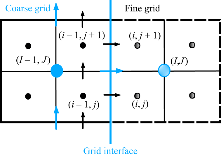
The detailed implementation of the above-summarized algorithm can be found in the original work by Manhart (Reference Manhart2004).


 Open access