


1. Introduction
Froth flotation, in which rising air bubbles are used for recovering hydrophobic particles, has been traditionally used in industry (Kitchener Reference Kitchener1984; Wills & Napier-Munn Reference Wills and Napier-Munn2006). However, this method is not efficient for particles smaller than approximately  $20\ \mathrm {\mu }$m, which, instead of being captured by the bubble, move around it (Mehrotra, Sastry & Morey Reference Mehrotra, Sastry and Morey1983; Barnocky & Davis Reference Barnocky and Davis1989; Loewenberg & Davis Reference Loewenberg and Davis1994; Miettinen, Ralston & Fornasiero Reference Miettinen, Ralston and Fornasiero2010). An alternative to froth flotation is provided by the more efficient hydrophobic oil-binder techniques (Sirianni, Capes & Puddington Reference Sirianni, Capes and Puddington1969; Mehrotra et al. Reference Mehrotra, Sastry and Morey1983; van Netten, Moreno-Atanasio & Galvin Reference van Netten, Moreno-Atanasio and Galvin2014, Reference van Netten, Moreno-Atanasio and Galvin2016). These methods, however, can be expensive due to the amount of oil required. The present project is motivated by a more recent particle-capture technique, which circumvents the limitations of froth flotation and oil-binder techniques (Galvin & van Netten Reference Galvin and van Netten2017; van Netten, Borrow & Galvin Reference van Netten, Borrow and Galvin2017). This method consists of using a binder containing droplets filled with saltwater and covered by thin, surfactant-stabilized, semi-permeable oil layers. The presence of salt inside the droplet results in an osmotic flow that increases particle capture.
Several works have used two-particle dynamics to characterize aggregation phenomena (e.g. Zeichner & Schowalter Reference Zeichner and Schowalter1977; Davis Reference Davis1984; Rother & Davis Reference Rother and Davis2001; Phan et al. Reference Phan, Nguyen, Miller, Evans and Jameson2003; Roure & Cunha Reference Roure and Cunha2018). In a recent work, Davis & Zinchenko (Reference Davis and Zinchenko2018) found both semi-analytical and asymptotic solutions (i.e. far field and near field) for the translational mobility functions (Batchelor & Green Reference Batchelor and Green1972b) for the relative motion of a solid particle and a semi-permeable drop interacting in creeping flow for linear external flows. In the work of Davis & Zinchenko (Reference Davis and Zinchenko2018), the collision rates were found in the absence of osmotic flow. However, it should be noted that their results regarding the collision rates, as well as the ones in the aforementioned studies, were obtained in a quasi-steady context, in the sense that they assume a steady-state pair distribution function.
The goal of the present work is to investigate the two-particle dynamics of a solid particle and an expanding semi-permeable drop in the presence of both osmotic flow and an external, extensional flow field. The numerical integration of the relative particle motion is performed using the mobility functions found in Davis & Zinchenko (Reference Davis and Zinchenko2018). The computational results from the numerical integration are used for calculating the particle–drop collision efficiency. Rather than making a quasi-steady assumption, we consider both the short-term dynamics, as the particle–drop pair distribution function is being established, and the long-term dynamics, as the drop expands. We compare our results with an analytical result for the collision efficiency at time zero and with the steady-state solution (in the case of non-expanding droplets) by Davis & Zinchenko (Reference Davis and Zinchenko2018).
The equivalence between our approach and the standard quasi-steady one relies on the expectation that, in the context of non-expanding droplets, an initially uniform probability distribution will eventually approach a steady state, as calculated by Batchelor & Green (Reference Batchelor and Green1972a). There are several works concerning the steady-state pair distribution function for shear and pure strain flows (e.g. Brady & Morris Reference Brady and Morris1997; Morris & Katyal Reference Morris and Katyal2002; Wilson Reference Wilson2005; Blanc et al. Reference Blanc, Lemaire, Meunier and Peters2013). These works use distinct approaches, ranging from experimental to theoretical. However, all of them focus on steady-state distributions. Although works such as Gadala-Maria & Acrivos (Reference Gadala-Maria and Acrivos1980) present some transient experiments, the transient regime of microstructure is rarely explored in the literature. Hence, in the present work, we provide a numerical solution of the transient pair distribution function for the case of a non-expanding droplet, which enables us to better explain the transient particle-capture rate in terms of the suspension microstructure. This solution, besides justifying the assumptions made in the work, provides an estimation of the time it takes to reach the steady state.
1.1. Problem description and drop growth
We consider the creeping motion of a solid spherical particle relative to a semi-permeable spherical droplet filled with saltwater in the presence of a linear flow at infinity. At the surface of the rigid particle, we consider both impenetrability and no-slip boundary conditions. At the drop interface, although we still consider a no-slip boundary condition, with the membrane allowed to rotate to remain torque-free, we allow the existence of a normal component of the fluid velocity, as the drop is semi-permeable. The relative velocity through the interface is described by Darcy's law as being proportional to the hydrodynamic pressure jump. We also assume continuity of velocity at the drop's interface and that changes in the viscosity and density of the fluid inside the drop due to the presence of salt are negligible. Details concerning analytical and asymptotic solutions for the hydrodynamic problem are provided by Davis & Zinchenko (Reference Davis and Zinchenko2018).
The normal component of the fluid velocity relative to the semi-permeable interface is given by Darcy's law
 \begin{equation} {-}(\boldsymbol{u} - \boldsymbol{u}_s)\boldsymbol{\cdot}\hat{\boldsymbol{n}} |_{S} = K (\varPi + {\rm \Delta} p), \end{equation}
where  $S$ represents the drop surface, $\hat {\boldsymbol {n}}$ is the outward unit normal vector, $K$ is the oil-layer or membrane permeability, $\varPi$ is the osmotic pressure, ${\rm \Delta} p$ is the jump in dynamic pressure across the thin oil layer at the drop interface, $\boldsymbol {u}_s$ is the velocity of the interface and $\boldsymbol {u}$ is the fluid velocity. The osmotic pressure for dilute solutions may be estimated by Van't Hoff's law
 \begin{equation} \varPi \approx RT c_s, \end{equation}
where  $c_s$ is the salt concentration near the drop's interior surface, $R$ is the ideal gas constant and $T$ is the absolute temperature. The pressure jump ${\rm \Delta} p$ is of order $\sim \mu \dot {\gamma }$, which is much smaller than the osmotic pressure jump $\varPi$ in typical cases. Here, $\mu$ is the fluid viscosity and $\dot {\gamma }$ is the intensity of the far-field extensional flow, whose undisturbed velocity field is given by $( \dot {\gamma } x, \dot {\gamma } y,-2\dot {\gamma }z)$.
As we are assuming flow of an incompressible liquid, the osmotic flow will result in an increase of the drop's size. To find the expansion rate of the drop, we note that the terms  $\boldsymbol {u}\boldsymbol {\cdot } \hat {\boldsymbol {n}}|_S$ and ${\rm \Delta} p$ in (1.1) cancel out due to the boundary conditions of the hydrodynamic problem. It is noted that the term $\varPi$ does not contribute to the velocity of the fluid at the boundary, as this extra source term would result in a violation of continuity, as the integral $\int _S \boldsymbol {u}\boldsymbol {\cdot }\hat {\boldsymbol {n}} \, \textrm {d} S$ at the drop's interface would be non-zero. Thus, as we consider the fluid motion to be quasi-stationary, as drop expansion happens slowly, the hydrodynamic problem at each time is reduced to the same one investigated by Davis & Zinchenko (Reference Davis and Zinchenko2018), with the same boundary conditions. Again, we refer to the aforementioned paper for the full analysis and solution of the hydrodynamic problem both outside and inside the drop. Considering that the interface velocity $\boldsymbol {u}_s = u_s \hat {\boldsymbol {e}}_r$ is purely radial, as the drop keeps its spherical shape, so $\hat {\boldsymbol {n}} = \hat {\boldsymbol {e}}_r$, the velocity of the interface is given by
 \begin{equation} u_s = K R T c_s. \end{equation}
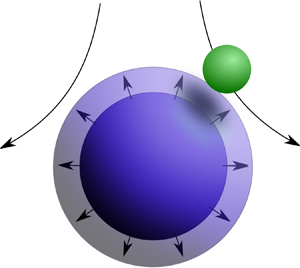
As the drop expands, its interface moves outward through the surrounding suspension, with velocity  $\boldsymbol {u}_s$, without modifying the fluid velocity $\boldsymbol {u}$, and it acts as a passive sieve that captures or engulfs the particles that it encounters in the suspension. Particles are also swept to this interface by the external flow, as shown in figure 1. From this point on, quantities are non-dimensional unless noted otherwise. For the non-dimensionalization of the problem, we use $a_{d0}$ as the length scale and $\dot {\gamma }^{-1}$ as the time scale, where $a_{d0}$ is the initial drop radius. Considering a small spherical drop with instant relaxation (i.e. in a regime of low Péclet numbers for the salt molecules), conservation of mass yields a differential equation for the non-dimensional drop radius
 \begin{equation} \textrm{d} a_d/\textrm{d} t = Eg \ a_d^{-3}, \end{equation}
where
 \begin{equation} Eg = K R T c_0/(\dot{\gamma} a_{d0}) \end{equation}
is the engulfment parameter, which represents the ratio between osmotic permeate flow and external convective flow and  $c_0$ is the initial salt concentration in the drop. The word engulfment here is used in analogy to the phenomenon in solidification where particles are engulfed by a solidifying or freezing moving interface (e.g. Omenyi & Neumann Reference Omenyi and Neumann1976; Asthana & Tewari Reference Asthana and Tewari1993; Stefanescu et al. Reference Stefanescu, Juretzko, Catalina, Dhindaw, Sen and Curreri1998; Mukherjee & Stefanescu Reference Mukherjee and Stefanescu2004). This parameter can also be thought as a ratio between the characteristic dimensional flow time $\tau _{\kern0.05em fl} = \dot {\gamma }^{-1}$ and the characteristic dimensional drop-expansion time $\tau _{eng} = a_{d0}/(K R T c_0)$. The engulfment parameter can be decomposed as $Eg = K^* c_0 R T / \mu \dot {\gamma }$, in which the first term is the non-dimensional permeability $K^* = K \mu / a_{d0}$, which is usually small (Davis & Zinchenko Reference Davis and Zinchenko2018), and the second term is the ratio between osmotic and viscous pressures, which is usually large. Thus, $Eg$ can take on a broad range of values. In particular, Davis & Zinchenko (Reference Davis and Zinchenko2018) noted that $\mu K \approx 10^{-4} \ \mathrm {\mu }\text {m}$ for microfiltration membranes, yielding $K^* = \mu K/a_{d0} \approx 10^{-6}\text{--}10^{-4}$ for $a_{d0} = 1\text {--}100 \ \mathrm {\mu }\text {m}$. Then, for $\mu = 0.01 \ \text {g}\ \text {cm-s}^{-1}, RTc_0 = 10^6 \ \text {g}\ \text {cm-s}^{-2}$ (i.e. $c_0 \approx 0.04 \ \text {M}$ at room temperature) and $\dot {\gamma } = 10^3 \ \text {s}^{-1}, Eg = 0.1\text {--}10$. As another example, Matsumoto et al. (Reference Matsumoto, Inoue, Kohda and Ikura1980) examined the swelling of small, oil-covered water drops and globules with $a_{d0} = 2\text {--}10 \ \mathrm {\mu }\text {m}, c_0 = 0.06\text {--}0.6 \ \text {M}$ and corresponding initial swelling rates of $K R T c_0 = {\textit{O}}(10^{-4}\text{--}10^{-3} \ \text {cm}\ \text {s}^{-1})$, from which $\mu K = {\textit{O}}(10^{-8} \ \mathrm {\mu }\text {m}), K^* = {\textit{O}}(10^{-9}\text{--}10^{-8})$ and $Eg \approx 0.1\text {--}10$ for very low shearing of $\dot {\gamma } = 1\ \textrm {s}^{-1}$. Corresponding permeabilities for the experiments of van Netten et al. (Reference van Netten, Borrow and Galvin2017) are thought to be somewhat higher, due to active water transport by micelles, but quantitative values are not available because swelling experiments with much larger binder fragments for their system exhibited diffusion limitations (DeIuliis et al. Reference DeIuliis, Sahasrabudhe, Davis and Galvin2020).
Schematic of a solid particle interacting with an expanding drop in an external extensional flow field.

For constant membrane permeabilities, (1.4) can be solved analytically, yielding
 \begin{equation} a_d(t) = (1 + 4 Eg \, t)^{1/4}. \end{equation}
From (1.6), the drop expands with time due to the osmotic flow. The flux across the drop interface, however, decreases with time due to dilution of the internal saltwater, resulting in a decrease of expansion effects at large times. The time it takes for expansion effects to become negligible can be estimated by a scaling argument. As pointed out before, the ratio between the osmotic and hydrodynamic pressure differences is of order  ${Eg}/(K^* a_d^3(t))$. Hence, for this ratio to be small, we should have $a_d(t) \gg ({Eg}/K^*)^{1/3}$. For rapid diffusion, $a(t) \sim (4 {Eg} \, t)^{1/4}$ at large times. Thus, for the hydrodynamic effects to dominate over osmotic ones, we should have $t \gg K^{*-4/3} {Eg}^{1/3}$, which can be quite large for $K^* \ll 1$ and $Eg = {\textit{O}}(1)$.
2. Two-particle dynamics
2.1. Kinematic equations
Following Batchelor & Green (Reference Batchelor and Green1972b), the general expression for the relative velocity between two smooth, spherical particles freely suspended in a linear flow field at small Reynolds number is
 \begin{equation} \boldsymbol{V} = \boldsymbol{\varOmega}^{\infty} \wedge \boldsymbol{r} + \boldsymbol{\mathsf{E}}^{\infty} \boldsymbol{\cdot} \boldsymbol{r} - \left[ A(r) \frac{\boldsymbol{rr}}{r^2} + B(r) \left( \boldsymbol{1} - \frac{\boldsymbol{rr}}{r^2} \right) \right]\boldsymbol{\cdot} \boldsymbol{\mathsf{E}}^{\infty}\boldsymbol{\cdot}\boldsymbol{r}, \end{equation}
where  $A(r)$ and $B(r)$ are the so-called mobility functions, $\boldsymbol {r}$ is the vector from the centre of the drop to the centre of the particle, $r = \|\boldsymbol {r}\|$ and $\boldsymbol {\varOmega }^{\infty }$ and $\boldsymbol{\mathsf{E}}^{\infty }$ are the undisturbed rotation vector and rate-of-strain tensor, respectively, for the far-field flow. These mobility functions arise in the solution of the hydrodynamic problem at low Reynolds number and are related to the intensity of hydrodynamic interaction between the particles, which cause them to deviate from the undisturbed flow streamlines. Both functions $A$ and $B$ vanish when the distance between the particle and the drop goes to infinity, as hydrodynamic interactions become weaker. For non-permeable surfaces, the quantity $1 - A$ goes to zero as the particle approaches the drop, which prevents contact in finite time, unless additional attractive forces are present. In contrast, the presence of a semi-permeable interface mitigates this lubrication resistance, allowing the particle and the drop to collide. In the context of the present problem, these functions depend on the non-dimensional permeability and the ratio between particle and drop radii (Davis & Zinchenko Reference Davis and Zinchenko2018). Although there is an implicit dependence of the mobility functions on the engulfment parameter and time (due to the changing radius ratio), there is no explicit dependence of the mobility functions on the expansion rate, as we are assuming the motion to be quasi-stationary for small Reynolds numbers (i.e. the diffusion of vorticity is much faster than the motion of the particles or the expansion rate). By definition of a pure extensional flow, the rotation vector is $\boldsymbol {\varOmega }^{\infty } = \boldsymbol {0}$ and the non-dimensional strain rate tensor at infinity is given by
 \begin{equation} \boldsymbol{\mathsf{E}}^{\infty} = \begin{bmatrix} 1 & 0 & 0 \\ 0 & 1 & 0 \\ 0 & 0 & -2 \end{bmatrix}. \end{equation}
Thus, in Cartesian components, the equations of motion are
 \begin{gather} {\textrm{d} x}/\textrm{d}t = (1 - B) x + E x, \end{gather}
 \begin{gather}{\textrm{d} y}/\textrm{d}t = (1 - B) y + E y, \end{gather}
 \begin{gather}\textrm{d}z/\textrm{d}t = - 2 (1 - B) z + E z, \end{gather}
where
 \begin{equation} E = (B - A) (x^2 + y^2 - 2 z^2)/r^2. \end{equation}
Note that the present set of differential equations is not autonomous for the case of an expanding drop, as the mobility functions depend on the decreasing ratio between the radii of the particle and drop, and, consequently, on time.
2.2. Particle trajectories
The numerical integration of the relative particle trajectories was performed using a fourth-order Runge–Kutta scheme. The exact solution of the hydrodynamic problem by Davis & Zinchenko (Reference Davis and Zinchenko2018) in terms of bi-spherical harmonics was used to evaluate the mobility functions. We also employed an adaptive time step at small gaps, to avoid particle-drop overlap in the intermediate Runge–Kutta steps. The drop-size evolution was described analytically by (1.6). As illustrated in figure 2, there are some initial conditions that lead to collision between the particle and the drop and others that do not. Hence, we perform several simulations for trajectories starting at varied initial positions to determine starting locations that lead to particle–drop collision within a certain time.
Trajectory simulation for  $Eg = 1.0, K^* = 10^{-4}, a_p = 0.5$ and $z_0 = 4.0$, with (a) $x_0 = 0.6$ and (b) $x_0 = 0.7$. The dashed line represents the final interface of the drop at the end of the trajectory. In $(a)$, the solid particle is captured by the expanding drop, whereas the trajectory in $(b)$ does not result in aggregation.

3. Collision efficiency
In this section, we start by showing the equivalence of the multiple definitions of the pair collision rate used in this work. Furthermore, we proceed to derive an analytical expression of the ideal pair collision rate between a particle with an expanding drop at time zero. This initial collision rate is used in latter sections to validate the numerical results for the collision efficiency.
3.1. Pair collision rates
The problem of calculating the rates at which two different species collide with one another is present in many branches of science, such as chemistry and colloidal sciences. In a classical point of view, this problem is closely related to the scenario of particles colliding with a surface. Namely, a particle will collide with another one when the surfaces make contact.
For a given surface  $S$ and given particle dynamics, we define $V_{col}(t;S)$ (the $S$ here will be usually omitted, reading $V_{col}(t)$) as the collisional volume of the surface $S$ in a time $t$. It is the volume in which every trajectory starting within this volume will result in a collision in a time smaller than $t$. By using this notation, the probability $\mathcal {P}_{col}(t)$ of a particle colliding with a surface $S$ in a time less than $t$ is given by the probability measure of a particle to be inside $V_{col}(t)$ at time equal zero. For two different species, we can compute the (average) total number of collisions between two species by multiplying the collisional probability $\mathcal {P}_{col}(t)$ by $N_1 N_2$, with $N_i$ being the total number of particles of species $i$, or, in the case of two particles of the same species, by $N (N-1)/2$. Hence, the general rate of pairwise collision between two species per unit volume is given by
 \begin{equation} J_{12} = n_1 n_2 \frac{\textrm{d}}{\textrm{d} t}\int_{V_{col}(t)} \tilde{f}(\boldsymbol{x}) \, \textrm{d} V, \end{equation}
where  $n_i$ is the number density of species $i$, and $\tilde {f}(\boldsymbol {x}) \equiv f(\boldsymbol {x},0)$ is the pair distribution function evaluated at $t = 0$. The unsteady state for $f(\boldsymbol {x},t)$ is governed by the Liouville equation (Batchelor & Green Reference Batchelor and Green1972a)
 \begin{equation} \frac{\partial f}{\partial t} + \boldsymbol{\nabla}\boldsymbol{\cdot}(\boldsymbol{V} f) = 0, \end{equation}
where  $\boldsymbol {V}$ is the relative velocity of the colliding species. For specific cases such as steady-state probability distributions, it is useful to use a modified version of Reynolds transport theorem to re-write the pair collision rate as a surface integral. We define $\tilde {\boldsymbol {V}}(\boldsymbol {x},t)$ as the velocity of the bounding surface of the collision volume. The lower portion of this surface is simply $S_{col}$, the original collision surface, as shown in figure 3, on which $\tilde {\boldsymbol {V}} = 0$. Hence, the pair collision rate is given by
 \begin{equation} J_{12} = n_1 n_2 \int_{A_{col}} \hat{\boldsymbol{n}} \boldsymbol{\cdot} \tilde{\boldsymbol{V}} \tilde{f}(\boldsymbol{x}) \, \textrm{d} A, \end{equation}
where  $A_{col}(t)$ is the upper or expanding portion of the collision surface (see figure 3), $\tilde {\boldsymbol {V}}$ is its velocity and $\hat {\boldsymbol {n}}$ is the outward unit normal to $A_{col}(t)$. The geometry of the problem for our specific context of collision of a particle with a spherical collision surface is illustrated in figure 3. Although (3.3) is general (i.e. it is valid for non-steady states), it is not very useful for unsteady states, given that the evaluation of $\tilde {\boldsymbol {V}}$ is not always straightforward. However, there are some properties of steady-state distributions that make this expression more useful. Namely, for a steady-state probability distribution, as the field $\boldsymbol {V}$ does not depend on time, the velocity $-\tilde {\boldsymbol {V}}$ coincides with the relative velocity $\boldsymbol {V}$ (note that $\boldsymbol {V}$ is inward, while $\tilde {\boldsymbol {V}}$ is outward) and $f(\boldsymbol {x},t) = f(\boldsymbol {x}) = \tilde {f}(\boldsymbol {x})$. Moreover, we can extend the collision area $A_{col}$ to infinity by using the continuity equation.
Illustration of the collision volume of a particle colliding with a collision surface  $S$. The shaded $S_{col}$ represents the portion of $S$ where particles are effectively captured, whereas the non-shaded region is where particles are pulled away from the drop by the extensional flow faster than the drop expands. In our specific case of a particle colliding with an expanding drop under an external pure extensional field, $S$ is a sphere of dimensionless radius $R = 1+ a_p$ (i.e. the original drop radius plus particle radius) and $S_{col}$ is located at the top and bottom of the sphere, starting at an elevation angle $\alpha$ to be determined. The collision volume $V_{col}(t)$ is the region composed of the starting positions that will lead to aggregation in a time less than or equal to $t$;
$t$;  $A_{col}(t)$ is the boundary of the collision volume with $S_{col}$ excluded. Although the drop expands in time, $S_{col}$ is kept fixed as $V_{col}$ smoothly increases, because $V_{col}(t)$ is the suspension volume at time zero from which all particles will be collected by time $t$.
$t$.

For a steady-state relative velocity field, the trajectories coincide with its integral curves. If we extend the collisional volume along a ‘streamtube’ of  $\boldsymbol {V}(\boldsymbol {x})$ that contains all the points inside the collisional volume extending toward infinity, by the divergence theorem and (3.2), the probability flux, defined as the integral in (3.3), is equal in every section of the extended volume. This fact allowed most researchers to focus their analysis on a collision section far from the reference particle, where $f(\boldsymbol {x}) \sim 1$. This consideration allows writing equation (3.3) for a steady-state probability distribution as
 \begin{equation} J_{12} = - n_1 n_2 \int_{A_{col}^{\infty}} \hat{\boldsymbol{n}} \boldsymbol{\cdot} \boldsymbol{V} \, \textrm{d} A, \end{equation}
where  $A_{col}^{\infty }$ is a section (typically a horizontal cross-section) of the extended collisional volume far from the reference particle. Equation (3.4) is a practical way to evaluate the collision efficiency, as it does not rely on previous knowledge of the pair distribution function (Zeichner & Schowalter Reference Zeichner and Schowalter1977; Davis Reference Davis1984; Davis & Zinchenko Reference Davis and Zinchenko2018). There are other works, such as Phan et al. (Reference Phan, Nguyen, Miller, Evans and Jameson2003), that compute the collision efficiency by evaluating the integral over $S_{col}$. However, in order to avoid using the probability distribution explicitly, they assume that the relative velocity $\boldsymbol {V}$ is a solenoidal field, which is often not the case.
Regarding the case in the absence of a steady-state distribution, for an initially uniform probability distribution (i.e.  $f(\boldsymbol {x},0) = 1$), the rate of collision between two different species per unit volume is given by
 \begin{equation} n_1 n_2 \, \textrm{d} V_{col}/ \textrm{d} t. \end{equation}
Equation (3.5) is essentially transient, as it assumes an initial distribution that is not at steady state, and, therefore, will only reach the steady-state collision efficiency if the chosen initial pair distribution also reaches a steady state. Throughout the subsequent sections, we show that this transient behaviour is indeed the case for non-expanding droplets. Furthermore, we define the collision efficiency as the ratio between the pair collision rate and the ideal collision rate, which was calculated by Zeichner & Schowalter (Reference Zeichner and Schowalter1977) by using (3.4) considering the case of rigid non-expanding spherical particles in an extensional flow in the absence of hydrodynamical interactions. This ideal collision rate is given by
 \begin{equation} J_{12}^{id} = n_1 n_2 \frac{8 {\rm \pi}}{3 \sqrt{3}} (a_1 + a_2)^3. \end{equation}
3.2. Important limiting cases
Physically, there are two distinct mechanisms that contribute to the capture of particles by expanding drops: convective capture due to the imposed flow and engulfment capture due to the drop's expansion. The interplay between these two mechanisms is characterized by the engulfment parameter  $Eg$, which was defined in the first section of the present paper. Here, we analyse the limits where $Eg = 0$ and $Eg \to \infty$.
In the first case, where  $Eg = 0$, the drop does not expand and the steady problem reduces to the one described in Davis & Zinchenko (Reference Davis and Zinchenko2018). For this case, the collision efficiency at steady state is solely due to flow and given by
 \begin{equation} E_{col}^{\,fl} = \frac{1}{\phi^3(R)}, \end{equation}
where the function  $\phi (r)$ involves an integral over the relative particle distance and is defined as
 \begin{equation} \phi(r) = \exp \left(\int_{r}^{\infty} \frac{A(r') - B(r')}{1 - A(r')} \frac{\textrm{d} r'}{r'}\right) . \end{equation}
 In the second limiting case, where  $Eg \to \infty$, the drop expands and flow effects are negligible. In this limit, particle capture due to pure expansion happens much faster than the particle motion, and, hence, relaxation of the probability distribution is negligible. Thus, we can use (1.6), (3.5) and (3.6) to derive the collision efficiency, resulting in
 \begin{equation} E_{col}^{exp}(t) = \frac{3 \sqrt{3}}{2} \frac{(a_d(t) + a_p)^2}{(1 + a_p)^3} \frac{{Eg}}{(a_d(t))^3}. \end{equation}
At large times, for  $a_d(t) \gg a_p$, this function slowly decays in proportion to $t^{-1/4}$, using (1.6). Of considerable practical importance is that the collision efficiency in this limit remains non-zero for $a_p \to 0$, whereas the collision efficiency for flow-induced capture becomes very small as $a_p \to 0$, due to hydrodynamic interactions.
3.3. Characteristic times and population dynamics at short times
At time zero, before any collection takes place, the only species present in the suspension are particles and drops. For simplicity, we consider that the particles are all of the same size and do not form agglomerates. In this case, the population dynamics for the particle phase is given by
 \begin{equation} \textrm{d} n_p/ \textrm{d} t = - J n_p n_d. \end{equation}
 When the particles are much smaller than the droplets, the capture of a single particle does not affect the capture efficiency of an additional particle by a given droplet. Hence, we can consider the resultant agglomerate as a single drop. In this case,  $n_d$ is a constant. By a scaling analysis of (3.10) and knowing that $J = \textrm {d} V_{col}/ \textrm {d} t$, the characteristic time of bulk capture is given by
 \begin{equation} \tau_{bulk} = T/(a_{d0}^3 n_d )= 4 {\rm \pi}T / (3 \phi_0), \end{equation}
where  $\phi _0 = 4 {\rm \pi}a_{d0}^3 n_d/3$ is the initial volume fraction of droplets and we choose the characteristic microscopic capture time $T$ to be
 \begin{equation} T = ( 1/\tau_{\kern0.05em fl} + 1/\tau_{eng} )^{-1}, \end{equation}
so that it scales with the smaller of the flow and engulfment times. Since  $\phi _0 \ll 1$ for dilute systems governed by pairwise interactions, the time scale for bulk capture of particles is long compared to the pairwise capture dynamics. Equation (3.10) can be solved analytically for an initially uniform pair distribution function, yielding (in non-dimensional quantities)
 \begin{equation} n_p = n_{p0} \exp(- V_{col}(t)/\tau), \end{equation}
where  $\tau = \tau _{bulk}/T$ is the ratio between the characteristic bulk capture time and microscopic capture time. Thus, $V_{col}(t)$ is as a direct measure of particle capture over time. For the practical systems discussed in § 1.1, the dimensional time scales are $\tau _{\kern0.05em fl} = \dot {\gamma }^{-1} = 10^{-3} \ \text {s}$ and $\tau _{eng} = a_{d0}/(KRT c_0) = 10^{-4}\text{--}10^{-2} \ \text {s}$ for the parameters cited by Davis & Zinchenko (Reference Davis and Zinchenko2018), and $\tau _{\kern0.05em fl} = 1 \ \text {s}$ and $\tau _{eng} = 0.1\text {--}10 \ \text {s}$ for the experiments of Matsumoto et al. (Reference Matsumoto, Inoue, Kohda and Ikura1980). For a dilute suspension with $\phi _0 \lessapprox 0.01, \tau _{bulk}$ is more than $100$-fold larger.
3.4. Initial rate of collision with an expanding drop
In this subsection, we derive an analytical solution for the initial rate of collision of a rigid spherical particle with an expanding drop, in the case of an initially uniform pair distribution function. This solution is then used in subsequent sections to confirm the transient results obtained via numerical simulations.
In the present problem, the relative radial velocity at the collisional surface at time zero (i.e. the surface of a sphere with radius  $R = 1 + a_p$) is, from (2.1) and (1.4),
 \begin{equation} V_{rel} = V_r - \frac{\textrm{d} a_d}{\textrm{d} t} = \frac{(1-A)}{(B-A)} E r - \frac{{Eg}}{a_{d}^3}. \end{equation}
At  $t = 0$, when $r = R = 1 + a_p$, the relative radial velocity is
 \begin{equation} V_{rel} = R (1 - A_0)(1- 3 \cos^2(\theta)) - {Eg}, \end{equation}
where  $A_0$ is the mobility function $A$ evaluated at the collisional radius $R$. Although $1 - A_0$ is zero for two solid particles, it has a non-zero value if one (or both) of the spheres is permeable, as noted by Davis & Zinchenko (Reference Davis and Zinchenko2018). To calculate the rate of collision, we need to restrict the domain of the collisional surface to the locations with negative relative velocity (so that the capture occurs). In this case,
 \begin{equation} \cos^2(\theta) > \frac{1}{3} \left( 1 - \frac{{Eg}}{R(1-A_0)} \right). \end{equation}
Thus, the domain of integration is restricted to  $\theta \in D = [0,\alpha ] \cup [{\rm \pi} - \alpha , {\rm \pi}]$, with
 \begin{equation} \alpha = \left\{\begin{array}{@{}ll} \arccos\left\{ \left[\dfrac{1}{3} \left( 1 - \dfrac{{Eg}}{R(1-A_0)} \right) \right]^{1/2} \right\}& \text{for ${Eg} < R(1 - A_0)$} \\ {\rm \pi}/ 2 & \text{for ${Eg} > R(1 - A_0)$} \end{array}\right. . \end{equation}
This domain is shown as the shaded area in figure 3. Therefore, for an initial uniform probability distribution, the integral in (3.3) at time zero is given by
 \begin{align} \int_{S_{col}} \tilde{\boldsymbol{V}} \boldsymbol{\cdot} \hat{\boldsymbol{n}} \, \textrm{d} S &= \int_{S_{col}} [{Eg} - R(1-A_0)(1 - 3 \cos^2(\theta))] \, \textrm{d} S \nonumber\\ &= S_{col} [ {Eg} - R(1 - A_0) ] + 12 {\rm \pi}R^3(1 - A_0) \int_{0}^{\alpha} \cos^2(\theta) \sin(\theta) \, \textrm{d} \theta \nonumber\\ &= 4 {\rm \pi}R^2 (1 - \cos(\alpha)) [ {Eg} - R(1 - A_0) ] + 4 {\rm \pi}R^3(1 - A_0) (1 - \cos^3(\alpha)). \end{align}
Dividing the collision rate at time zero by the ideal collision rate (3.6) yields the initial collision efficiency
 \begin{equation} E_{col}(0) = \frac{3 \sqrt{3}}{2} \left[ \frac{{Eg}}{R} (1 - \cos(\alpha)) + (1 - A_0) (\cos(\alpha) - \cos^3(\alpha))\right], \end{equation}
where  $\alpha$ is given by (3.17). For engulfment values larger than $R(1- A_0)$, all the cosines in (3.19) vanish, indicating that the collision efficiency for these cases is initially dominated entirely by expansion. In other words, the expansion is then fast enough to capture particles on all parts of the drop surface at time zero, even in regions where the extensional flow pulls particles away from the drop.
Figure 4 shows a plot of the initial collision efficiency versus the engulfment parameter for several values of the non-dimensional permeability. The results for  $Eg = 0$ are
 \begin{equation} E_{col}(0) |_{{Eg} = 0} = \frac{3 \sqrt{3}}{2} (1 - A_0)(\cos(\alpha) - \cos^3(\alpha)). \end{equation}
The collision efficiency for  $K^* = 0$ is necessarily zero in this limit, for which $A_0 = 1$, due to lubrication preventing the contact of impermeable spheres (when, at least, one of them is solid) in a finite time under the action of finite forces (Barnocky & Davis Reference Barnocky and Davis1989). However, the collision efficiency quickly increases in the presence of even small permeabilities. The initial collision efficiency, then, increases as $Eg$ increases, due to the increasing role of engulfment aiding the convective capture due to the extensional flow.
Initial collision efficiency versus the engulfment parameter for  $a_p = 0.5$ and different values of non-dimensional permeability. The solid line represents the limit where $K^* \to 0$, and, hence, $(1 - A_0) = 0$.

In the opposite limit of  $Eg \gg 1, \alpha = {\rm \pi}/2$ and the initial collision from (3.19) is simply
 \begin{equation} E_{col}(0) = 3 \sqrt{3} \ {Eg}/(2R). \end{equation}
The initial collision efficiency then increases linearly with the engulfment parameter and is independent of permeability (other than the dependence of the engulfment parameter on permeability per (1.5)). Equation (3.21) corresponds to the solid line for  $K^* = 0$ with $R = 1.5$ in figure 4. Moreover, from (3.9) and using (1.6), the collision efficiency for pure engulfment ( $Eg \gg 1$) is
 \begin{equation} E_{col}(t) = \frac{3 \sqrt{3} [ (1 + 4 {Eg} t)^{1/4} + a_p ]^{2} {Eg} }{2(1+a_p)^3 (1+4 {Eg} t)^{3/4}}, \end{equation}
valid for all times. Equation (3.22) reduces to (3.21) for  $t = 0$, using $R = 1 + a_p$. As noted before, the collision efficiency in this limit also remains finite for small particles ( $a_p \ll 1$).
3.5. Transient microstructure and collision efficiency
In this section, we provide a numerical solution of the transient pair distribution function  $f(\boldsymbol {x},t)$. This solution can be used to better understand the transient behaviour of the collision efficiency of a particle with a non-expanding drop.
The pair distribution function is governed by (3.2). Considering the motion of a particle relative to a non-expanding droplet, for which the vector field  $\boldsymbol {V}$ given by (2.1) is in a steady state, (3.2) can be re-written as (Batchelor & Green Reference Batchelor and Green1972a)
 \begin{equation} \frac{\textrm{D}}{\textrm{D}t} \left( \frac{f(\boldsymbol{r},t)}{q(r)} \right) = 0, \end{equation}
where  $\textrm {D}/\textrm {D}t = \partial /\partial t + \boldsymbol {V} \boldsymbol {\cdot } \boldsymbol {\nabla }$ and $q(r)$ is given by $(1-A)^{-1} \phi ^{-3}(r)$. Hence, for an initially uniform pair density function, (3.23) can be solved by the method of characteristics, yielding
 \begin{equation} f(\boldsymbol{r},t) = \frac{q(r)}{q(R(\boldsymbol{x},t))}, \end{equation}
where  $R(\boldsymbol {x},t)$ is the radial component of the starting position $\boldsymbol {R}$ that ends in $\boldsymbol {x}$ at time $t$. Due to the kinematic reversibility characteristic of Stokes flows, $\boldsymbol {R}(\boldsymbol {x},t)$ can be evaluated using the inverse flux of the dynamical equations. It should be noted that the solution by the method of characteristics is only valid at points for which the position at time $t$ can be traced back to an initial point in space. That means the collision volume of the inverse dynamics represents a particle depletion region adjacent to the collision surface. This region is also referred as wake region by Wilson (Reference Wilson2005). For points away from the wake region, where the particles come from infinity, we have $\lim _{t \to \infty } q(R(\boldsymbol {x},t)) = 1$, and, thus, the pair distribution function approaches $q(r)$ at large times, which is the analytical result given by Batchelor & Green (Reference Batchelor and Green1972a).
Coupling the analytical transient solution given by (3.24) with our trajectory simulations, we were able to find numerical values for the pair distribution function, which are displayed in figure 5 for  $K^* = 10^{-4}$ and $a_p = 0.5$, at $t = 0.25, 0.75, 1.0$ and $1.5$. From these results, we see the formation of the wake region near the $xy$ plane, which increases outward in time as the probability distribution approaches a steady state. Moreover, although the wake region continues to increase with time, comparison with the theoretical steady state shows that the pair distribution function away from this wake region becomes close to the theoretical steady state for $t = {\textit{O}}(1)$.
Numerical results for the transient pair distribution function for a rigid particle and a non-expanding permeable drop at distinct times. The values for the non-dimensional permeability and particle radius are  $K^* = 10^{-4}$ and $a_p = 0.5$, at times (a) $t = 0.25$, (b) $t = 0.75$, (c) $t = 1.0$ and (d) $t = 1.5$. The white region surrounding the origin is the excluded volume bounded by the collision surface.

On the upper region of the collision sphere, we can see an increase of the pair distribution function with time. This increase physically means that there is a higher probability of encountering a particle at this region, which results in an increase of the probability flux, and, hence, the collision efficiency should increase with time until it reaches a steady state.
4. Numerical results and discussion
In this section, we present the results of numerical computation of the collision efficiency. We start with the shapes of the collision volumes, which were obtained by numerical interpolation of the collision time as a function of starting position. We then present results on the change of the collision volume and collision efficiency with time.
4.1. Collision boundaries
The collision boundaries are, by definition, the level surfaces of the function  $t_{col}(\boldsymbol {x}_0)$ (i.e. the collision time of a certain trajectory starting at a point $\boldsymbol {x}_0$). Using data from multiple trajectory simulations, we obtained numerical values for these boundaries by numerical interpolation of the data for $t_{col}(\boldsymbol {x}_0)$, which are found by calculating multiple trajectories for different starting positions. As an example, figure 6 shows the collision boundaries for different values of $t$ and $Eg = 1$. Note that, as $t$ increases, the collision surface converges to a limit surface, except near the axis of symmetry, where there will be a collision tube as $t \to \infty$. In the absence of engulfment, this limit curve should be the same as the one predicted by Davis & Zinchenko (Reference Davis and Zinchenko2018).
Collision boundaries for  $Eg = 1.0, K^* = 10^{-4}, a_p = 0.5$, and (in to out) $t = 0.02, 0.1, 0.3, 0.5, 0.7, 0.9$ and $1.0$. The inset shows a zoom of the details of the right region of the graph, where the curves start to coincide. The shaded region represents the inside of the collision surface $r = 1 + a_p$. The collision volume ( $V_{col}$) is the unshaded region between the collision surface ( $S_{col}$) and the collision boundary ( $A_{col}$).

For non-expanding drops, the regular interpolation method fails to obtain some of the points on the collision boundary next to the drop at larger times, due to computational time constraints, as particle capture takes longer in the absence of drop expansion. Thus, in these cases, we used an auxiliary method that makes use of the fact that, for a stationary field  $\boldsymbol {V}(\boldsymbol {r})$, points on $A_{col}$ change in time with velocity $-\boldsymbol {V}(\boldsymbol {r})$. Thus, the inverse flux of the original dynamical system gives us a homotopy between surfaces $S_{col}$ and $A_{col}$ (i.e. we can continuously deform one surface into the other). Numerically, we permeate points throughout $S_{col}$ and evolve them using the velocity $-\boldsymbol {V}(\boldsymbol {r})$, which helps construct $A_{col}$.
The shapes of the collision boundaries displayed in figure 6 result from the interplay between the flow and expansion mechanisms. The different shapes of the collision volume for  $t = 0.5$ are shown in figure 7 for the cases of pure flow, pure expansion and combination of both effects. Due to the extensional flow, in which the flow is toward the drop near the axis of symmetry and away from the drop near the equator, non-expanding droplets display a lateral region in which particles are not captured. For engulfment parameters higher than $R(1-A_0)$, this region ceases to exist (See (3.17)) and, instead, there is a finite capture layer that results from the balance between drop-expansion effects (which decay with time) and pulling of particles away from the drop due to the extensional flow.
Different geometries of the collision volume for  $t = 0.5$ and $K^* = 10^{-4}$. The combined case and pure expansion consider $Eg = 1.0$.

4.2. Collision efficiency
Using knowledge about the collision boundaries, together with their symmetry about the  $z-$axis, we are able to calculate the collision volume numerically for distinct points in time using a simple trapezoidal method. Moreover, to validate our results, we use the analytical solution in (3.18) to predict the initial slope of the curve $V_{col}(t)$. Figure 8 shows the collision volume versus time for engulfment parameters $Eg = 0$, $0.125, 0.25, 0.5$ and $1.0$ for $a_p = 0.5$ and $K^* = 10^{-4}$. The values shown in figure 8 $(a)$ correspond to the actual values of the collision efficiency, whereas the values in 8 $(b)$ are normalized by the initial slope, which was calculated using (3.19) combined with the definition of collision efficiency. The dashed line in figure 8 $(b)$ is a straight line starting at the origin with unit slope. The collision volume grows noticeably faster for larger values of $Eg$, which indicates a larger collision efficiency. The normalization in 8 $(b)$ allows us to perceive a transition in behaviour as the engulfment number increases. There is a transition of patterns at short times, which occurs at values of engulfment near $0.5$. Namely, as the engulfment number increases, the collision volume curves transition from a flow-like behaviour to an expansion-like one (represented by the shaded region in figure 8). By examining the slopes of the curves in figure 8, we see that, for small values of $Eg$, the collision efficiency initially increases with time. In contrast, for $Eg = 1$, although the initial value is much larger, the collision efficiency decreases at short times. This decrease can be explained by the dominance of the expansion mechanism in the collision efficiency for large engulfment parameters, which slows with time due to dilution of the saltwater inside the drop, resulting in a reduction in the collision efficiency.
Collision volume increase with time for  $K^* = 10^{-4}, a_p = 0.5$ and engulfment parameters of $Eg = 0, 0.125, 0.25, 0.5$ and $1.0$. Here, $(a)$ shows the values for the collision volume, whereas the values in $(b)$ are normalized by their initial slopes predicted by the analytical solution for the initial collision rate. The solid curves represent the results obtained by numerical integration. The dashed line in $(b)$ is a straight line with unit slope. The shaded area in $(b)$ represents the region in which particle capture is dominated by expansion at short times.

The numerical values for the collision efficiency were obtained by numerical differentiation of  $V_{col}(t)$, according to (3.5). To reduce the numerical noise due to interpolation, we applied a smoothing spline to the collision volume function before taking the numerical derivative. The results for the collision efficiency obtained by this numerical differentiation are shown in figure 9. Note that the results agree with the prediction from the analytical solution for time zero. Moreover, in the case of a non-expanding droplet, the solution reaches a steady state with a numerical value close to the one predicted by Davis & Zinchenko (Reference Davis and Zinchenko2018) (as indicated by the dashed line on the top right of figure 9 $a$). As expected by the results and discussion in § 3.5, the collision efficiency increases monotonically as it approaches a steady state within a time near unity, due to the particles slowing down as they approach the drop, and, thus, building up in concentration. However, our results indicate that, even for small values of the engulfment parameter, the collision efficiency is much larger than for pure flow ( $Eg =0$). Another interesting feature is that, for small engulfment parameters such as $Eg = 0.25$, the shape of the collision efficiency curve is similar to the one without expansion. However, it should be noted that even small values of $Eg$ can increase the collision efficiency by several times. Furthermore, from figure 9 $(d)$, increasing the engulfment parameter results in a shape transition from a monotonically increasing curve to a decaying behaviour that is closer to the one observed in the pure expansion efficiency given by (3.9). For $Eg = 1$, the hydrodynamic and engulfment and flow time scales, $\tau _{eng}$ and $\tau _{\kern0.05em fl}$, are of the same order, and, thus, there is a substantial contribution of the far-field flow in particle capture, as the external flow drags particles closer to the drop, which is reflected, among other things, on the collision volume shape (see figure 7) and explains the difference between the curves. Moreover, engulfment dominates for short times when $Eg = 1$, but then the difference between the numerical results and the pure engulfment approximation deviate at longer times as engulfment slows and convective capture becomes more important. For larger values of $Eg$, as $\tau _{eng} > \tau _{\kern0.05em fl}$, the solution becomes closer to the pure expansion solution in (3.9) and (3.22), as can be seen in the inset of figure 9 $(d)$.
Numerical results for the transient collision efficiency versus time for  $K^* = 10^{-4}, a_p = 0.5$ and engulfment parameters (a) $Eg = 0$, (b) $Eg = 0.25$, (c) $Eg = 0.5$, (d) $Eg = 1.0$ and $7.0$ (in inset). The dashed lines represent the analytical solution at $t = 0$, and the value of the theoretical steady-state collision efficiency in $(a)$. The dashed curve in $(d)$ is the pure expansion collision efficiency, as described by (3.9) and (3.22).

We further validate our numerical results by simulating the non-expanding case for different values of non-dimensional permeability  $K^*$. The results concerning the collision efficiency for different values of permeability are displayed in figure 10. The numerical results for different permeabilities match within $0.01$ with both theoretical solutions for steady-state and initial collision efficiencies.
Numerical results for the transient collision efficiency with respect to time for  $Eg = 0, a_p = 0.5$ and different values of non-dimensional permeability: $K^* = 10^{-2}, K^* = 10^{-3}, K^* = 10^{-4}$ and $K^* = 10^{-5}$. The dashed lines represent the theoretical results for the initial and steady-state collision efficiencies.

We also plotted the results for different permeabilities in the case of expanding droplets (i.e.  $Eg \ne 0$). The results for these simulations are displayed in figure 11 for values of the engulfment parameter (a) $Eg = 0.25$ and (b) $Eg = 1.0$. Figure 11 shows that the differences between the values of collision efficiency for different values of $K^*$ shown in figure 10 are mitigated with an increase of the engulfment parameter. The results displayed in figure 11 $(b)$ show that the increase of $Eg$ results in the collapse of curves for different small permeabilities into a single limit curve. In this regime, engulfment is the primary capture mechanism, and the collision efficiency is governed by particle expansion and the external flow far from the drop, which drags particles close to the drop so that they will be captured by engulfment.
Numerical results for the transient collision efficiency with respect to time for (a)  $Eg = 0.25$, (b) $Eg = 1.0$. The results are for $a_p = 0.5$ and different values of non-dimensional permeability: $K^* = 10^{-4}, K^* = 10^{-5}$ and $K^* = 10^{-6}$. The dashed lines represent the theoretical results for the initial collision efficiency. The dashed curve in $(b)$ is the pure expansion collision efficiency. For high values of $Eg$, the system becomes less sensitive to changes in permeability and the curves collapse onto a single curve.

Another parameter that is important in the determination of collision efficiency is the non-dimensional particle radius. As mentioned before, previous works (e.g. Barnocky & Davis Reference Barnocky and Davis1989; Loewenberg & Davis Reference Loewenberg and Davis1994) show that particle capture is hindered for small particle sizes. As shown in Davis & Zinchenko (Reference Davis and Zinchenko2018), the presence of permeability increase capture efficiency at smaller radii. In fact, as we now show, the presence of particle engulfment further increases this efficiency. Figure 12 shows results for the transient collision efficiency for different values of particle radii,  $K^* = 10^{-4}$ and $Eg = 0.25$. Due to the high influence of engulfment over particle capture and the $1/R$ dependence of the engulfment-dominated collision efficiency (cf., (3.21) and (3.22)), the decrease in particle radius, in contrast to non-expanding cases, causes an increase in the collision efficiency at short times. However, by normalizing the results by the initial collision efficiency, as displayed in figure 12 $(b)$, we see that the increase of particle radius from $0.25$ to $1.0$ results in a larger percentage increase of the collision efficiency, given that such increase is caused by flow effects.
Numerical results for the transient collision efficiency for  $Eg = 0.25, K^* = 10^{-4}$ and different values of particle radii: $a_p = 0.25, a_p = 0.5$ and $a_p = 1.0$. Here, $(a)$ shows the values for the transient collision efficient, whereas, in $(b)$, the results are normalized by the numerical value for the initial collision efficiency. The dashed lines represent the theoretical results for the initial and steady-state collision efficiencies.

The strong effect of engulfment is demonstrated in a quantitative fashion in table 1. Here, the collision efficiency at  $t = 1$ is normalized with the steady-state collision efficiency for flow only, $E_{col}^* = E_{col}/E_{col}^{\,fl}$, for systems with the same dimensionless size ratio and permeability. For the conditions in this table, the increase in collision efficiency is roughly 3–18 fold. The highest values occur at lower permeability, smaller particle radius and higher engulfment parameter, as expected. It is also noteworthy that the largest increase occurs for small particles (which are the most difficult to capture).
Relative collision efficiency  $E_{col}^*$ at time $t = 1$ for $Eg = 0, 0.25, 0.5$ and $1.0$. The first two result columns show the relative collision efficiency for $a_p = 0.5$ for distinct permeabilities, whereas the last three result columns show the relative collision efficiency for $K^* = 10^{-4}$ for different particle radii.

5. Concluding remarks
We investigated the interaction between an expanding spherical droplet and a solid particle in an external extensional flow. Using the results of relative particle trajectories obtained via numerical simulation, we calculated the transient collision efficiencies for different parameter values. Further, we derived an analytical expression for the initial collision efficiency and numerical results for the pair distribution function.
In contrast with previous works (e.g. Zeichner & Schowalter Reference Zeichner and Schowalter1977; Davis Reference Davis1984; Davis & Zinchenko Reference Davis and Zinchenko2018; Roure & Cunha Reference Roure and Cunha2018), we have not restricted our analysis to a steady-state pair distribution function. Rather, by starting with a uniform pair distribution, we demonstrated the evolution of the collision efficiency at short times. We applied the numerical solutions of the relative dynamics of the rigid particle to find a numerical solution of the transient pair distribution function for the case of non-expanding droplets. This solution allowed us to investigate the transiency of the collision efficiency and the time it takes to reach a steady state. For non-expanding droplets, the collision efficiency increases with time and approaches the steady state predicted by Davis & Zinchenko (Reference Davis and Zinchenko2018). The time it takes for the system to reach a steady state is of order  $\dot {\gamma }^{-1}$ and agrees with our microstructure simulations, which also explain the monotonically increasing behaviour of the collision efficiency for these cases. The monotonicity, however, can be broken in the presence of engulfment.
The numerical results for the collision efficiency, obtained by numerical differentiation of the collision volume with respect to time, agree with theoretical results for both initial and steady-state collision efficiencies. Drop-expansion effects decay slowly with time, as engulfment capture slows with time due to a decrease in the osmotic driving force, as the internal saltwater is diluted. Overall, drop-expansion effects contribute to the increase of collision efficiency even for small values of the engulfment parameter  $Eg$. Of particular importance is that engulfment capture is relative insensitive to particle size, and so is particularly effective relative to convective capture for small particles. Further increase of $Eg$ results in a transition from a flow-dominated behaviour of the collision efficiency, with a monotonically increasing curve to a engulfment-dominated behaviour, where the collision efficiency decreases with time. At high values of $Eg$, the system becomes less sensitive to changes in the permeability, which indicates the predominance of the far-field flow and engulfment as the predominant capture mechanisms in these cases.
Funding
Acknowledgment is made to the donors of The American Chemical Society Petroleum Research Fund for partial support of this research. This work was also supported, in part, by a seed grant from the University of Colorado and a grant from the Australian Research Council (grant no. DP180101617, which is now covered by grant CE2000100009).
Declaration of interest
The authors report no conflict of interest.


 Open access