


1. Introduction
It has long been postulated that there is a coupling between the spontaneous polarisation of ferroelectric liquid crystals and an applied electric field (Clark & Lagerwall Reference Clark and Lagerwall1980; Lagerwall Reference Lagerwall2004); as a consequence, this has led to a resurgence of interest in these materials (Pleiner & Brand Reference Pleiner and Brand1999; Calderer & Joo Reference Calderer and Joo2008; Guo et al. Reference Guo, Yan, Chigrinov, Zhao and Tribelsky2019). This paper is concerned with the electromechanical effects that can arise from flow-induced movement of the liquid crystal.
Jákli et al. (Reference Jákli, Bata, Buka, Éber and Jánossy1985), Járkli & Saupe (Reference Járkli and Saupe1991) and Jákli (Reference Jákli1997) reported that a ferroelectric smectic C $^{\ast }$
(SmC*) liquid crystal sample exhibiting bookshelf-type alignment can vibrate laterally under the influence of an applied electric field when placed between two horizontal plates, where the lower plate is fixed and the upper plate is free to move. Jákli & Saupe (Reference Jákli and Saupe1995) also discovered, in contrast to Jákli et al. (Reference Jákli, Bata, Buka, Éber and Jánossy1985), Járkli & Saupe (Reference Járkli and Saupe1991) and Jákli (Reference Jákli1997), that a fast electric field reversal can induce vertical vibrations; see also Jákli & Saupe (Reference Jákli and Saupe1996).
$^{\ast }$
(SmC*) liquid crystal sample exhibiting bookshelf-type alignment can vibrate laterally under the influence of an applied electric field when placed between two horizontal plates, where the lower plate is fixed and the upper plate is free to move. Jákli & Saupe (Reference Jákli and Saupe1995) also discovered, in contrast to Jákli et al. (Reference Jákli, Bata, Buka, Éber and Jánossy1985), Járkli & Saupe (Reference Járkli and Saupe1991) and Jákli (Reference Jákli1997), that a fast electric field reversal can induce vertical vibrations; see also Jákli & Saupe (Reference Jákli and Saupe1996).
In order to understand this phenomenon from a theoretical perspective, Stewart (Reference Stewart2010) started with a continuum theory of fluids in which the viscous behaviour of the material is assumed to play a more important role than the elastic properties (Jákli et al. Reference Jákli, Bata, Buka, Éber and Jánossy1985), an approach that had previously been adopted in Jákli & Saupe (Reference Jákli and Saupe1996). Employing a simple ansatz for the velocity of the liquid crystal, given later in this paper by (4.1), Stewart (Reference Stewart2010) was then able to demonstrate this so-called pumping phenomenon qualitatively. The ansatz itself was motivated by the review of Leslie (Reference Leslie1992) and the work of Clark et al. (Reference Clark, Saunders, Shanks and Leslie1981) that examined oscillatory shear effects in nematic liquid crystals, with the form of the ansatz being such that the incompressibility condition was satisfied and the viscous stress tensor turned out to be identically zero. However, one drawback of the ansatz was that the no-slip condition cannot be satisfied at one of the plates, arbitrarily chosen to be the moving one, although it was argued by Stewart (Reference Stewart2010) that this might not be a cause for concern since the adopted profile velocity constitutes a qualitatively reasonable approximate form for the anticipated flow. Thus, the purpose of this paper is to determine what happens when Stewart’s ansatz is not used, but the velocity is found by using the full equations for the balance of angular and linear momentum. Moreover, although the original experiments in Jákli & Saupe (Reference Jákli and Saupe1995) were three-dimensional, we follow Stewart (Reference Stewart2010) in considering a two-dimensional (2-D) model. However, whereas both fast field reversal and the effect of an alternating electric field were considered in Stewart (Reference Stewart2010), here we investigate only the first of these and defer the second to future work: this is because taking account of fast field reversal alone in a more complete manner requires a far lengthier exposition. In view of the slender geometry in the original geometry, i.e. a thin layer of liquid crystal, we formulate and analyse a time-dependent squeeze-film model, akin to that in the classical slider bearing problem and in the modelling of flow in Hele-Shaw cells (Acheson Reference Acheson1990; Morrow et al. Reference Morrow, Moroney, Dallaston and McCue2021; Chandaragi et al. Reference Chandaragi, Shetty, Choudhari, Vaidya and Prasad2025); indeed, it is only fairly recently that there has been any concerted study of the Hele-Shaw flows of nematic liquid crystals (nematics), both experimentally and theoretically (Cousins et al. Reference Cousins, Wilson, Mottram, Wilkes and Weegels2019, Reference Cousins, Bhadwal, Corson, Duffy, Sage, Brown, Mottram and Wilson2023, Reference Cousins, Bhadwal, Mottram, Brown and Wilson2024a , Reference Cousins, Mottram and Wilson2024b ; Sengupta et al. Reference Sengupta, Pieper, Enderlein, Bahr and Herminghaus2013a , Reference Sengupta, Tkalec, Ravnik, Yeomans, Bahr and Herminghaus2013b ). Furthermore, the current problem turns out to be akin to an oscillatory squeeze flow (OSF) for a non-Newtonian fluid, wherein the fluid is driven periodically by the motion of one of the confining, parallel planes; this type of setting exists in some devices using magnetorheological fluids (Li et al. Reference Li, Mu, Sun, Li and Wang2018) or electrorheological fluids (Wingstrand et al. Reference Wingstrand, Alvarez, Hassager and Dealy2016), where the fluid is squeezed periodically under a variable magnetic or electric field, as a means of achieving continuously variable control of mechanical vibrations, and is also envisioned as a mode of achieving control over transport in confined systems (Yang et al. Reference Yang, Christov, Griffiths and Ramon2020). An early theoretical analysis of OSF for viscoelastic fluids was conducted by Phan-Thien & Tanner (Reference Phan-Thien and Tanner1983), who provided analytical solutions for the velocity profile and the normal force required to drive the plate; for more recent work, see Yang et al. (Reference Yang, Christov, Griffiths and Ramon2020) and Mederos et al. (Reference Mederos, Bautista, Méndez and Arcos2024). However, the current context is slightly different, in that the fluid motion is not driven by the periodic forcing of one of the plates, but by an electric field; moreover, we find that the bounding plate that is free to move undergoes an oscillatory motion, albeit damped, even though the electric field itself is not oscillatory.
The layout of the paper is as follows. In § 2 we provide a brief description of SmC* liquid crystals, followed by the governing equations for the problem in § 3. In § 4 we recap the approach employed in Stewart (Reference Stewart2010), although providing a non-dimensional interpretation that was not present in the original work. In § 5 the full model equations are non-dimensionalised and then asymptotically reduced to give a leading-order model; analysis of this model follows in § 6. The results are given in § 7 and conclusions are drawn in § 8.
2. SmC* description
We employ a standard description of SmC $^{\ast }$
liquid crystals and consider a sample consisting of equidistant layers between two horizontal parallel plates in a so-called bookshelf alignment, where the layers are arranged perpendicular to the plates (Stewart Reference Stewart2004). A unit vector
$^{\ast }$
liquid crystals and consider a sample consisting of equidistant layers between two horizontal parallel plates in a so-called bookshelf alignment, where the layers are arranged perpendicular to the plates (Stewart Reference Stewart2004). A unit vector $\boldsymbol{n}$
, called the director, is inclined at an angle
$\boldsymbol{n}$
, called the director, is inclined at an angle $\theta$
to the unit layer normal
$\theta$
to the unit layer normal $\boldsymbol{a}$
, as displayed in figure 1(a). In the case of SmC
$\boldsymbol{a}$
, as displayed in figure 1(a). In the case of SmC $^{\ast }$
liquid crystals, the director can maintain a relative tilt to the smectic layers while being free to rotate around the surface of a fictitious cone of semi-vertical angle
$^{\ast }$
liquid crystals, the director can maintain a relative tilt to the smectic layers while being free to rotate around the surface of a fictitious cone of semi-vertical angle $\theta$
, often referred to as the smectic cone angle; see figure 1(b). It is assumed that
$\theta$
, often referred to as the smectic cone angle; see figure 1(b). It is assumed that $\theta$
is fixed to be constant, so that the incompressible flow theory of Leslie, Stewart & Nakagawa (Reference Leslie, Stewart and Nakagawa1991) may be applied. It is convenient to introduce the unit vector
$\theta$
is fixed to be constant, so that the incompressible flow theory of Leslie, Stewart & Nakagawa (Reference Leslie, Stewart and Nakagawa1991) may be applied. It is convenient to introduce the unit vector $\boldsymbol{c}$
(known as the cvector), which is the unit orthogonal projection of
$\boldsymbol{c}$
(known as the cvector), which is the unit orthogonal projection of $\boldsymbol{n}$
onto the smectic planes, and the unit vector
$\boldsymbol{n}$
onto the smectic planes, and the unit vector $\boldsymbol{b}=\boldsymbol{a}\times \boldsymbol{c}$
. Ferroelectric liquid crystals are chiral in nature and, in general, possess a spontaneous polarisation,
$\boldsymbol{b}=\boldsymbol{a}\times \boldsymbol{c}$
. Ferroelectric liquid crystals are chiral in nature and, in general, possess a spontaneous polarisation, $\boldsymbol{P}$
: this can be written as a vector parallel to the vector
$\boldsymbol{P}$
: this can be written as a vector parallel to the vector $\boldsymbol{b}$
, so that
$\boldsymbol{b}$
, so that
 \begin{align} \boldsymbol{P}=P_{0}\boldsymbol{b},\phantom {space}P_{0}\gt 0, \end{align}
when the sign of $P_{0}$
is taken to be positive, as displayed in figure 1(b). The vectors
$P_{0}$
is taken to be positive, as displayed in figure 1(b). The vectors $\boldsymbol{b}$
and
$\boldsymbol{b}$
and $\boldsymbol{c}$
are orthogonal to each other and always lie in the plane of the smectic layers, perpendicular to
$\boldsymbol{c}$
are orthogonal to each other and always lie in the plane of the smectic layers, perpendicular to $\boldsymbol{a}$
as shown in figure 1(b). When there are no dislocations, it is well known that the smectic layer normal,
$\boldsymbol{a}$
as shown in figure 1(b). When there are no dislocations, it is well known that the smectic layer normal, $\boldsymbol{a}$
, is such that
$\boldsymbol{a}$
, is such that $\boldsymbol{\nabla }\times \boldsymbol{a}=0$
(Oseen Reference Oseen1933). This constraint is automatically satisfied when
$\boldsymbol{\nabla }\times \boldsymbol{a}=0$
(Oseen Reference Oseen1933). This constraint is automatically satisfied when $\boldsymbol{a}$
=
$\boldsymbol{a}$
= $\boldsymbol{i}$
(unit vector along the
$\boldsymbol{i}$
(unit vector along the $x$
axis) for planar layers as set out in figure 1(a). For fixed planar aligned layers, the orientation of the cdirector can be described by introducing the phase angle
$x$
axis) for planar layers as set out in figure 1(a). For fixed planar aligned layers, the orientation of the cdirector can be described by introducing the phase angle $\phi$
, which is defined to be the angle between the cdirector and the
$\phi$
, which is defined to be the angle between the cdirector and the $y$
axis measured in the positive direction; see figure 1(c). The problem consists of smectic layers, perpendicular to two horizontal parallel plates placed initially at a sample depth,
$y$
axis measured in the positive direction; see figure 1(c). The problem consists of smectic layers, perpendicular to two horizontal parallel plates placed initially at a sample depth, $h_{0}$
, apart in the
$h_{0}$
, apart in the $z$
direction, with the vector
$z$
direction, with the vector $\boldsymbol{a}$
being parallel to the
$\boldsymbol{a}$
being parallel to the $x$
axis. The lower plate is fixed and the upper plate is free to move. The width of the sample in the
$x$
axis. The lower plate is fixed and the upper plate is free to move. The width of the sample in the $y$
direction is initially
$y$
direction is initially $b_{0}$
, as are the widths of the plates. The electric field is applied across the plates in the negative
$b_{0}$
, as are the widths of the plates. The electric field is applied across the plates in the negative $z$
direction, as shown in figure 1(c). One possible initial equilibrium state at time
$z$
direction, as shown in figure 1(c). One possible initial equilibrium state at time $t=0$
is shown in figure 1(c) where the electric field is
$t=0$
is shown in figure 1(c) where the electric field is $\boldsymbol{E}=-E\boldsymbol{k}$
with
$\boldsymbol{E}=-E\boldsymbol{k}$
with $E=|\boldsymbol{E}|$
and
$E=|\boldsymbol{E}|$
and $\phi =\pi$
. For
$\phi =\pi$
. For $t\gt 0,$
the electric field is then reversed so that
$t\gt 0,$
the electric field is then reversed so that $\boldsymbol{E}=E\boldsymbol{k}$
. The sample can then experience a field-induced change, as shown schematically in figure 2 for a single representative smectic layer.
$\boldsymbol{E}=E\boldsymbol{k}$
. The sample can then experience a field-induced change, as shown schematically in figure 2 for a single representative smectic layer.
(a) The initial configuration of a bookshelf-aligned SmC* liquid crystal. The short, bold lines represent the local alignment of the director when it is inclined at a fixed angle $\theta$
relative to the local smectic layer normal. (b) The local geometrical description of the director
$\theta$
relative to the local smectic layer normal. (b) The local geometrical description of the director $\boldsymbol{n}$
, layer normal
$\boldsymbol{n}$
, layer normal $\boldsymbol{a}$
, spontaneous polarisation
$\boldsymbol{a}$
, spontaneous polarisation $\boldsymbol{P}$
and the vector
$\boldsymbol{P}$
and the vector $\boldsymbol{c}$
, the unit orthogonal projection of the director upon the smectic planes. Here
$\boldsymbol{c}$
, the unit orthogonal projection of the director upon the smectic planes. Here $\boldsymbol{n}$
is tilted at a fixed angle
$\boldsymbol{n}$
is tilted at a fixed angle $\theta$
to the layer normal
$\theta$
to the layer normal $\boldsymbol{a}=\boldsymbol{i}$
, the unit vector in the
$\boldsymbol{a}=\boldsymbol{i}$
, the unit vector in the $x$
direction. The angle
$x$
direction. The angle $\phi$
describes the orientation of
$\phi$
describes the orientation of $\boldsymbol{c}$
within the plane of the layers relative to the
$\boldsymbol{c}$
within the plane of the layers relative to the $y$
axis. (c) One possible initial configuration when an electric field is applied in the negative
$y$
axis. (c) One possible initial configuration when an electric field is applied in the negative $z$
direction, so that
$z$
direction, so that $\boldsymbol{P}$
is aligned with the field and the corresponding orientation angle of
$\boldsymbol{P}$
is aligned with the field and the corresponding orientation angle of $\boldsymbol{c}$
is
$\boldsymbol{c}$
is $\phi =\pi$
.
$\phi =\pi$
.

Geometrical description of a single representative incompressible SmC* layer under a fast electric field reversal. (a) At $t=0,$
the height of the layer is
$t=0,$
the height of the layer is $h_{0}$
and the width is
$h_{0}$
and the width is $b_{0}$
. (b) Under a field reversal, the top plate may move, leading to a change in the shape of the sample. To maintain a fixed volume of fluid, the area of the representative layer must effectively remain constant. Any increase in height must be accompanied by a corresponding decrease in the width, so that (3.4) is satisfied. Figure not drawn to scale.
$b_{0}$
. (b) Under a field reversal, the top plate may move, leading to a change in the shape of the sample. To maintain a fixed volume of fluid, the area of the representative layer must effectively remain constant. Any increase in height must be accompanied by a corresponding decrease in the width, so that (3.4) is satisfied. Figure not drawn to scale.

3. Governing equations
An electric field is imposed across the positive $z$
direction. As mentioned in § 2, it is known that the height of the liquid crystal sample will increase with time. In deriving what is a moving-boundary initial-value problem, only the following smectic viscosities are included in the stress tensor (Stewart Reference Stewart2010):
$z$
direction. As mentioned in § 2, it is known that the height of the liquid crystal sample will increase with time. In deriving what is a moving-boundary initial-value problem, only the following smectic viscosities are included in the stress tensor (Stewart Reference Stewart2010): $\mu _{0},\mu _{3},\mu _{4},\lambda _{2}$
and
$\mu _{0},\mu _{3},\mu _{4},\lambda _{2}$
and $\lambda _{5}$
. Finally, we assume that this is a 2-D problem; thus, there is no flow in the
$\lambda _{5}$
. Finally, we assume that this is a 2-D problem; thus, there is no flow in the $x$
direction. Following the usual convention, we shall assume that the velocity of the liquid crystal is
$x$
direction. Following the usual convention, we shall assume that the velocity of the liquid crystal is $\boldsymbol{v}=(v,w)$
, its density is
$\boldsymbol{v}=(v,w)$
, its density is $\rho$
and its pressure is
$\rho$
and its pressure is $p$
. We shall now provide the incompressibility equations, the equations of linear and angular momentum and the equation of motion for the upper plate, as well as the boundary and initial conditions.
$p$
. We shall now provide the incompressibility equations, the equations of linear and angular momentum and the equation of motion for the upper plate, as well as the boundary and initial conditions.
3.1. Incompressibility
Assuming incompressibility for the liquid crystal, we must have
 \begin{equation} \frac {\partial v}{\partial y}+\frac {\partial w}{\partial z}=0. \end{equation}
Moreover, although we assume that the liquid crystal sample will originally occupy $-b_{0}/2\le y\le b_{0}/2$
and
$-b_{0}/2\le y\le b_{0}/2$
and $0\le z\le h_{0},$
we can expect that, at a later time
$0\le z\le h_{0},$
we can expect that, at a later time $t,$
it will occupy
$t,$
it will occupy
 \begin{align} -\!\big ( b_{0}-b\big ( z,t\big) \big) /2\le y\le \big ( b_{0}-b\big ( z,t\big) \big) /2,\quad 0\le z\le h_{0}+h( t) , \end{align}
where $b,z\gt 0,$
whence we will require that
$b,z\gt 0,$
whence we will require that
 \begin{equation} h_{0}b_{0}=\int _{0}^{h_{0}+h( t) }\big ( b_{0}-b\big ( z^{\prime },t\big) \big) \mathrm{d}z^{\prime }, \end{equation}
as a direct result of mass conservation. Most generally, it is therefore possible that the upper plate will overhang the sample as the electric field is reversed. However, if we assume that $b$
does not depend on
$b$
does not depend on $z,$
as was done in Stewart (Reference Stewart2010) and is indicated in figure 2, and that
$z,$
as was done in Stewart (Reference Stewart2010) and is indicated in figure 2, and that $b\ll b_{0},$
we obtain
$b\ll b_{0},$
we obtain
 \begin{equation} b(t)=\dfrac {b_{0}\,h(t)}{h_{0}+h(t)}, \end{equation}
whence
 \begin{equation} \dot {b}(t)=\dfrac {b_{0}h_{0}\dot {h}(t)}{(h_{0}+h(t))^{2}}, \end{equation}
where the dot denotes differentiation with respect to time. We show later that, even in this paper where we do not employ the ansatz of Stewart (Reference Stewart2010), (3.3) will reduce to (3.4), to a good approximation.
3.2. Angular momentum and linear momentum
From Leslie et al. (Reference Leslie, Stewart and Nakagawa1991), we may express the conservation of angular momentum in terms of $\phi$
, the angle of the cdirector relative to the
$\phi$
, the angle of the cdirector relative to the $y$
axis, as
$y$
axis, as
 \begin{align} 2\lambda _{5}\,\frac {\mathrm{D}\phi }{\mathrm{D}t} & =-P_{0}\,E\,\sin \phi \nonumber \\ &\quad + \lambda _{2}\left [ \left ( \frac {\partial v}{\partial y}-\frac {\partial w}{\partial z}\right) \sin 2\phi -\left ( \frac {\partial v}{\partial z} +\frac {\partial w}{\partial y}\right) \cos 2\phi \right] \nonumber \\ &\quad - \lambda _{5}\left ( \frac {\partial v}{\partial z}-\frac {\partial w}{\partial y}\right)\! , \end{align}
where $\mathrm{D}/\mathrm{D}t$
denotes the material derivative and is given by
$\mathrm{D}/\mathrm{D}t$
denotes the material derivative and is given by
 \begin{align} \frac {\mathrm{D}}{\mathrm{D}t}=\frac {\partial }{\partial t}+v\frac {\partial }{\partial y}+w\frac {\partial }{\partial z}. \end{align}
Again, by appealing to the paper of Leslie et al. (Reference Leslie, Stewart and Nakagawa1991), or using directly the constitutive relations shown in Appendix A, we are able to obtain the $y$
and
$y$
and $z$
components of linear momentum, i.e.
$z$
components of linear momentum, i.e.
 \begin{align} \rho \frac {\mathrm{D}v}{\mathrm{D}t} & =-\frac {\partial p}{\partial y} +\frac {\partial }{\partial y}\bigg \{\mu _{0}\,\frac {\partial v}{\partial y} +\mu _{3}\,\cos ^{2}\phi \left [ \frac {\partial v}{\partial y}\cos ^{2}\phi +\frac {\partial w}{\partial z}\sin ^{2}\phi \right . \notag\\ &\quad\left .+\frac {1}{2}\left ( \frac {\partial v}{\partial z}+\frac {\partial w}{\partial y}\right) \sin 2\phi \right] +\ 2\mu _{4}\left [ \frac {\partial v}{\partial y}\cos \phi +\frac {1}{2}\left ( \frac {\partial v}{\partial z}+\frac {\partial w}{\partial y}\right) \sin \phi \right] \cos \phi \nonumber \\& \quad -\lambda _{2}\left [ \frac {\mathrm{D}\phi }{\mathrm{D}t}+\frac {1}{2}\left ( \frac {\partial v}{\partial z}-\frac {\partial w}{\partial y}\right) \right] \sin 2\phi \bigg \} +\frac {\partial }{\partial z}\bigg \{\frac {1}{2}\mu _{0}\left ( \frac {\partial v}{\partial z}+\frac {\partial w}{\partial y}\right) \notag\\ &\quad+\frac {1}{2}\mu _{3} \sin 2\phi \left [ \frac {\partial v}{\partial y}\cos ^{2}\phi +\frac {\partial w}{\partial z}\sin ^{2}\phi +\frac {1}{2}\left ( \frac {\partial v}{\partial z}+\frac {\partial w}{\partial y}\right) \sin 2\phi \right] \nonumber \\ &\quad +\ \frac {1}{2}\mu _{4}\left ( \frac {\partial v}{\partial z}+\frac {\partial w}{\partial y}\right) +\ \lambda _{2}\left [ \left ( \frac {\mathrm{D}\phi }{\mathrm{D}t}+\frac {\partial v}{\partial z}\right) \cos 2\phi -\frac {1} {2}\left ( \frac {\partial v}{\partial y}-\frac {\partial w}{\partial z}\right) \sin 2\phi \right] \nonumber \\ &\quad +\lambda _{5}\left [ \frac {\mathrm{D}\phi }{\mathrm{D}t}+\frac {1}{2}\left ( \frac {\partial v}{\partial z}-\frac {\partial w}{\partial y}\right) \right] \bigg \}, \end{align}
 \begin{align} \rho \frac {\mathrm{D}w}{\mathrm{D}t} & =-\frac {\partial p}{\partial z}-\rho g +\ \frac {\partial }{\partial y}\bigg \{\frac {1}{2}\mu _{0}\left ( \frac {\partial v}{\partial z}+\frac {\partial w}{\partial y}\right) \notag\\ &\quad+\frac {1}{2}\mu _{3}\sin 2\phi \left [ \frac {\partial v}{\partial y}\cos ^{2}\phi +\frac {\partial w}{\partial z}\sin ^{2}\phi +\frac {1}{2}\left ( \frac {\partial v}{\partial z}+\frac {\partial w}{\partial y}\right) \sin 2\phi \right] \nonumber \\ &\quad +\ \frac {1}{2}\mu _{4}\left ( \frac {\partial v}{\partial z}+\frac {\partial w}{\partial y}\right) +\lambda _{2}\left [ \frac {\mathrm{D}\phi }{\mathrm{D}t}\cos 2\phi +\frac {1} {2}\left ( \frac {\partial v}{\partial z}-\frac {\partial w}{\partial y}\right) \cos 2\phi \right. \notag\\ &\quad\left. +\frac {1}{2}\left ( \frac {\partial v}{\partial y}-\frac {\partial w}{\partial z}\right) \sin 2\phi -\frac {1}{2}\left ( \frac {\partial v}{\partial z}+\frac {\partial w}{\partial y}\right) \cos 2\phi \right] \nonumber \\ &\quad -\lambda _{5}\left [ \frac {\mathrm{D}\phi }{\mathrm{D}t}+\frac {1}{2}\left ( \frac {\partial v}{\partial z}-\frac {\partial w}{\partial y}\right) \right] \bigg \}\nonumber \\ &\quad +\frac {\partial }{\partial z}\bigg \{\mu _{0}\,\frac {\partial w}{\partial z}+\mu _{3}\left [ \frac {\partial v}{\partial y}\cos ^{2}\phi +\frac {\partial w}{\partial z}\sin ^{2}\phi +\frac {1}{2}\left ( \frac {\partial v}{\partial z}+\frac {\partial w}{\partial y}\right) \sin 2\phi \right] \sin ^{2} \phi \nonumber \\ &\quad +\ 2\mu _{4}\left [ \frac {\partial w}{\partial z}\sin \phi +\frac {1}{2}\left ( \frac {\partial v}{\partial z}+\frac {\partial w}{\partial y}\right) \cos \phi \right] \sin \phi \nonumber \\ &\quad +\lambda _{2}\left [ \frac {\mathrm{D}\phi }{\mathrm{D}t}+\frac {1}{2}\left ( \frac {\partial v}{\partial z}-\frac {\partial w}{\partial y}\right) \right] \sin 2\phi \bigg \}, \end{align}
respectively, where $g$
is the acceleration due to gravity.
$g$
is the acceleration due to gravity.
3.3. Equation of the motion of the top plate
To obtain the equation of motion of the top plate, we have, from Newton’s second law,
 \begin{equation} m_{\!p}\frac {\mathrm{d}^{2}h}{\mathrm{d}t^{2}}=-\int\!\! \int _{A}\left ( t_{33} +p_{a}\right) _{z=h_{0}+h(t)}\mathrm{d}y\mathrm{d}x, \end{equation}
where $A$
is the area of the plate,
$A$
is the area of the plate, $m_{\!p}$
is its mass and
$m_{\!p}$
is its mass and $p_{a}$
is the force per unit area exerted on the upper boundary of the plate, i.e. atmospheric pressure, and
$p_{a}$
is the force per unit area exerted on the upper boundary of the plate, i.e. atmospheric pressure, and $t_{33}$
is the appropriate component of the stress tensor. From (A1), we have
$t_{33}$
is the appropriate component of the stress tensor. From (A1), we have
 \begin{equation} t_{33}=-p+\tilde {t}_{33}, \end{equation}
with
 \begin{align} \tilde {t}_{33} & =\mu _{0}\,\frac {\partial w}{\partial z}+\mu _{3}\left [ \frac {\partial v}{\partial y}\cos ^{2}\phi +\frac {\partial w}{\partial z} \sin ^{2}\phi +\frac {1}{2}\left ( \frac {\partial v}{\partial z}+\frac {\partial w}{\partial y}\right) \sin 2\phi \right] \sin ^{2}\phi \nonumber \\ &\quad +\ 2\mu _{4}\left [ \frac {\partial w}{\partial z}\sin ^{2}\phi +\frac {1} {4}\left ( \frac {\partial v}{\partial z}+\frac {\partial w}{\partial y}\right) \sin 2\phi \right] \nonumber \\ &\quad +\ \lambda _{2}\left [ \frac {\mathrm{D}\phi }{\mathrm{D}t}+\frac {1}{2}\left ( \frac {\partial v}{\partial z}-\frac {\partial w}{\partial y}\right) \right] \sin 2\phi . \end{align}
For a square plate, as was the case in the original experiment in Jákli & Saupe (Reference Jákli and Saupe1995), (3.10) becomes
 \begin{equation} m_{\!p}\frac {\mathrm{d}^{2}h}{\mathrm{d}t^{2}}=-b_{0}\int _{-\frac {1}{2} \,(b_{0}-b(t))}^{\frac {1}{2}\,(b_{0}-b(t))}\left ( t_{33}+p_{a}\right) _{z=h_{0}+h(t)}\mathrm{d}y. \end{equation}
Thus, assuming symmetry about $y=0,$
we have
$y=0,$
we have
 \begin{align} -\frac {1}{2}\left ( \frac {m_{\!p}}{b_{0}}\right) \,\frac {\mathrm{d}^{2} h}{\mathrm{d}t^{2}} & =\int _{0}^{\frac {1}{2}\,(b_{0}-b(t))}\bigg (\mu _{0}\,\frac {\partial w}{\partial z} +\mu _{3}\left [ \frac {\partial v}{\partial y}\cos ^{2}\phi +\frac {\partial w}{\partial z}\sin ^{2}\phi \right . \notag\\ &\quad\left . +\frac {1}{2}\left ( \frac {\partial v}{\partial z}+\frac {\partial w}{\partial y}\right) \sin 2\phi \right] \sin ^{2}\phi + 2\mu _{4}\left [ \frac {\partial w}{\partial z}\sin ^{2}\phi \right . \notag\\ &\quad\left .+\frac {1} {4}\left ( \frac {\partial v}{\partial z}+\frac {\partial w}{\partial y}\right) \sin 2\phi \right] \nonumber \\ &\quad + \lambda _{2}\left [ \frac {\mathrm{D}\phi }{\mathrm{D}t}+\frac {1}{2}\left ( \frac {\partial v}{\partial z}\quad-\frac {\partial w}{\partial y}\right) \right] \sin 2\phi \bigg)_{z=h_{0}+h(t)}\mathrm{d}y \notag\\ &\quad-\int _{0}^{\frac {1}{2}\,(b_{0} -b(t))}\left ( p-p_{a}\right) _{z=h_{0}+h(t)}\mathrm{d}y. \end{align}
3.4. Boundary and initial conditions
The boundary conditions are then
 \begin{align} v=0,\quad w=0\quad \text{at }z=0,\quad 0\le y\le \frac {1}{2}\,(b_{0} -b(t)), \end{align}
which describe no slip and no normal flow, respectively;
 \begin{align} v=0,\quad \frac {\partial w}{\partial y}=0\quad \text{at }y=0,\quad 0\le z\le h_{0}+h(t), \end{align}
i.e. symmetry conditions;
 \begin{align} v=-\frac {1}{2}\frac {\mathrm{d}b}{\mathrm{d}t},\quad \,\frac {\partial w}{\partial y}=0,\quad p=p_{a}\quad \text{at }y=\frac {1}{2} \,(b_{0}-b(t)),\quad 0\le z\le h_{0}+h(t), \end{align}
i.e. the normal velocity component equals the velocity of the crystal/air interface, zero shear stress and atmospheric pressure, respectively;
 \begin{align} v=0,\ \quad w=\frac {\mathrm{d}h}{\mathrm{d}t}\quad \text{at }z=h_{0} +h(t),\quad 0\le y\le \frac {1}{2}\,(b_{0}-b(t)), \end{align}
which accounts for no slip and the fact that the liquid crystal remains attached to the plate and moves vertically with it, respectively. We also comment that, as in Stewart (Reference Stewart2010), we do not apply any type of anchoring condition to $\phi$
at
$\phi$
at $z=0$
and
$z=0$
and $h_{0}+h(t).$
As for the initial conditions, we have, at $t=0$
,
$t=0$
,
 \begin{align} v=0,\quad w=0, \end{align}
i.e. no velocity;
 \begin{align} h=0,\ \quad \frac {\mathrm{d}h}{\mathrm{d}t}=0, \end{align}
with the second of these indicating that the plate is initially stationary;
 \begin{equation} \phi =\phi _{0}\left ( y,z\right)\! . \end{equation}
In (3.21) we allow for a more general initial condition than in Stewart (Reference Stewart2010), where the only possibility that was considered was $\phi _{0}=\pi .$
Strictly speaking, what was actually considered was
$\phi _{0}=\pi .$
Strictly speaking, what was actually considered was
 \begin{equation} \phi _{0}=\pi -\varepsilon , \end{equation}
where $\varepsilon$
was a small strictly positive constant; we shall return to the significance of this modification later in § 6.2.
$\varepsilon$
was a small strictly positive constant; we shall return to the significance of this modification later in § 6.2.
4. Stewart’s analysis of fast field reversal
In this section, by employing Stewart’s ansatz for the velocity of the liquid crystal sample, we show that Stewart’s results, which were computed numerically, can be recovered analytically using asymptotic arguments.
Setting
 \begin{align} v=k( t) y,\quad w=-k( t) z, \end{align}
it follows that (3.1) is satisfied automatically; in addition, assuming that $\phi =\phi ( t) ,$
(3.6) becomes, at
$\phi =\phi ( t) ,$
(3.6) becomes, at $z=h_{0}+h(t)$
,
$z=h_{0}+h(t)$
,
 \begin{equation} 2\lambda _{5}\frac {\mathrm{d}\phi }{\mathrm{d}t}=-P_{0}E\sin \phi -\frac {4\lambda _{2}}{h_{0}+h( t) }\sin \phi \cos \phi \frac {\mathrm{d} h}{\mathrm{d}t}, \end{equation}
where we have employed the relationship
 \begin{equation} k(t)=-\frac {1}{h_{0}+h(t)}\frac {\mathrm{d}h}{\mathrm{d}t}, \end{equation}
which itself is obtained from (3.18b ) and (4.1b ).
The equations of balance of linear momentum, (3.8) and (3.9), are
 \begin{align} \rho \left ( \frac {\mathrm{d}k}{\mathrm{d}t}+k^{2}(t)\right) y & =-\frac {\partial p}{\partial y}, \end{align}
 \begin{align} \rho \left (\!-\frac {\mathrm{d}k}{\mathrm{d}t}+k^{2}(t)\right) z & =-\frac {\partial p}{\partial z}-\rho g; \end{align}
this is by virtue of the fact that the viscous terms vanish, thanks to the form of the ansatz. Integrating (4.4) and (4.5) with respect to $y$
and
$y$
and $z,$
respectively, we obtain
$z,$
respectively, we obtain
 \begin{align} p & =-\frac {1}{2}\rho \left ( \frac {\mathrm{d}k}{\mathrm{d}t}+k^{2} (t)\right) y^{2}+F_{1}\left ( z,t\right)\! , \end{align}
 \begin{align} p & =-\frac {1}{2}\rho \left (\! -\frac {\mathrm{d}k}{\mathrm{d}t}+k^{2} (t)\right) z^{2}+F_{2}\left ( y,t\right) -\rho gz, \end{align}
respectively, where $F_{1} ( z,t)$
and
$F_{1} ( z,t)$
and $F_{2} ( y,y)$
are arbitrary functions. In order that (4.6) and (4.7) are consistent with each other, we must have
$F_{2} ( y,y)$
are arbitrary functions. In order that (4.6) and (4.7) are consistent with each other, we must have
 \begin{equation} p=-\frac {1}{2}\rho \frac {\mathrm{d}k}{\mathrm{d}t}\big ( y^{2}-z^{2}\big) -\frac {1}{2}\rho k^{2}(t)\big ( y^{2}+z^{2}\big) -\rho gz+F_{3}( t) ; \end{equation}
in Stewart (Reference Stewart2010), $F_{3} ( t)$
is taken to be
$F_{3} ( t)$
is taken to be $p_{a}+\rho gh_{0}.$
Proceeding with
 \begin{equation} p=-\frac {1}{2}\rho \frac {\mathrm{d}k}{\mathrm{d}t}\big ( y^{2}-z^{2}\big) -\frac {1}{2}\rho k^{2}(t)\big ( y^{2}+z^{2}\big) +\rho g\big ( h_{0}-z\big) +p_{a}, \end{equation}
the equation for the motion of the top plate, (3.14), becomes, following Stewart (Reference Stewart2010),
 \begin{align} \rho _{p}\frac {\mathrm{d}^{2}h}{\mathrm{d}t^{2}} & =\frac {1}{2}\rho \left ( \frac {1}{12}\frac {b_{0}^{2}h_{0}^{2}}{\left ( h_{0}+h( t) \right) ^{3}}-\left ( h_{0}+h( t) \right) \right) \frac {\mathrm{d}^{2}h}{\mathrm{d}t^{2}}-\frac {1}{12}\frac {\rho b_{0}^{2} h_{0}^{2}}{\left ( h_{0}+h( t) \right) ^{4}}\left ( \frac {\mathrm{d}h}{\mathrm{d}t}\right) ^{2}\nonumber \\ &\quad -\frac {1}{h_{0}+h( t) }\big [ \mu _{0}+\mu _{3}\big ( \sin ^{2}\phi -\cos ^{2}\phi \big) \sin ^{2}\phi +2\mu _{4}\sin ^{2}\phi \big] \frac {\mathrm{d}h}{\mathrm{d}t} \notag\\&\quad -2\lambda _{2}\sin \phi \cos \phi \frac {\mathrm{d}\phi }{\mathrm{d}t}-\rho gh, \end{align}
where $\rho _{p}=m_{\!p}/b_{0}^{2}.$
Now, although the equations were not non-dimensionalised in Stewart (Reference Stewart2010), it is instructive to consider their dimensionless form, and we therefore do so here. We non-dimensionalise with
 \begin{equation} \tilde {t}=\frac {t}{[t] },\quad \tilde {h}=\frac {h}{[h] }, \end{equation}
where $ [ h]$
and
$ [ h]$
and $ [ t]$
are scales for
$ [ t]$
are scales for $h$
and
$h$
and $t$
that are still to be determined. Equations (4.2) and (4.10) become, on dropping the tildes,
$t$
that are still to be determined. Equations (4.2) and (4.10) become, on dropping the tildes,
 \begin{equation} 2\left ( \frac {\lambda _{5}}{\lambda _{2}}\right) \frac {\mathrm{d}\phi }{\mathrm{d}t}=-\left \{ \frac {P_{0}E[t] }{\lambda _{2}}\right \} \sin \phi -\frac {4\delta }{\big ( 1+\delta h\big) }\sin \phi \cos \phi \frac {\mathrm{d}h}{\mathrm{d}t}, \end{equation}
 \begin{align} \frac {\mathrm{d}^{2}h}{\mathrm{d}t^{2}} & =\frac {1}{2}\varGamma \left ( \frac {1}{12}\frac {1}{\big ( 1+\delta h\big) ^{3}}-\epsilon ^{2}\big ( 1+\delta h\big) \right) \frac {\mathrm{d}^{2}h}{\mathrm{d}t^{2}}-\frac {\delta \varGamma }{12\big ( 1+\delta h\big) ^{4}}\left ( \frac {\mathrm{d}h}{\mathrm{d} t}\right) ^{2}\nonumber \\ &\quad -\left \{ \frac {\mu _{0} [ t] }{\rho _{p} [ h ] }\right \} \frac {\delta }{1+\delta h}\big [ 1+\bar {\mu }_{3}\big ( \sin ^{2}\phi -\cos ^{2}\phi \big) \sin ^{2}\phi +2\bar {\mu }_{4}\sin ^{2}\phi \big] \frac {\mathrm{d}h}{\mathrm{d}t}\nonumber \\ &\quad -2\left \{ \frac {\lambda _{2}[t] }{\rho _{p}[h] }\right \} \sin \phi \cos \phi \frac {\mathrm{d}\phi }{\mathrm{d}t}-\left \{ \frac {\rho g[t] ^{2}}{\rho _{p}}\right \} h, \end{align}
respectively, where
 \begin{align} \delta =\frac {[h] }{h_{0}},\quad \epsilon =\frac {h_{0}}{b_{0} },\quad \varGamma =\frac {\rho b_{0}^{2}}{h_{0}\rho _{p}},\quad \bar {\mu }_{3} =\frac {\mu _{3}}{\mu _{0}},\quad \bar {\mu }_{4}=\frac {\mu _{4}}{\mu _{0} }; \end{align}
for later use, we also introduce
 \begin{align} \bar {\lambda }_{2}=\frac {\lambda _{2}}{\mu _{0}},\quad \bar {\lambda }_{5} =\frac {\lambda _{5}}{\mu _{0}}. \end{align}
Model parameters.

Using the data in table 1, we note that
 \begin{align} \epsilon \approx 1.7\times 10^{-4},\quad \varGamma \approx 5.5\times 10^{3},\quad \bar {\mu }_{3}\approx 0.5,\quad \bar {\mu }_{4}\approx 2.7; \end{align}
thus, we proceed with $\epsilon \ll 1,$ $\varGamma \gg 1,$ $\bar {\mu }_{3}\sim O ( 1) ,\bar {\mu }_{4}\sim O ( 1) .$
In addition, if we assume for the time being that
$\bar {\mu }_{3}\sim O ( 1) ,\bar {\mu }_{4}\sim O ( 1) .$
In addition, if we assume for the time being that $\delta \ll 1,$
(4.12) and (4.13) reduce, at leading order, to
$\delta \ll 1,$
(4.12) and (4.13) reduce, at leading order, to
 \begin{equation} 2\frac {\mathrm{d}\phi }{\mathrm{d}t}=-\left \{ \frac {P_{0}E[t] }{\lambda _{5}}\right \} \sin \phi , \end{equation}
 \begin{align} 0 & =\frac {\varGamma }{24}\frac {\mathrm{d}^{2}h}{\mathrm{d}t^{2}}-\left \{ \frac {\mu _{0}[t] }{\rho _{p}[h] }\right \} \delta \big [ 1+\bar {\mu }_{3}\big ( \sin ^{2}\phi -\cos ^{2}\phi \big) \sin ^{2}\phi +2\bar {\mu }_{4}\sin ^{2}\phi \big] \frac {\mathrm{d}h} {\mathrm{d}t}\nonumber \\ &\quad -2\left \{ \frac {\lambda _{2}[t] }{\rho _{p}[h] }\right \} \sin \phi \cos \phi \frac {\mathrm{d}\phi }{\mathrm{d}t}-\left \{ \frac {\rho g[t] ^{2}}{\rho _{p}}\right \} h, \end{align}
respectively; note that we retain the term in (4.18) containing $\delta$
since the overall size of this term has yet to be ascertained, as
$\delta$
since the overall size of this term has yet to be ascertained, as $ [ t]$
and
$ [ t]$
and $ [ h]$
have not yet been determined. Equations (4.17) and (4.18) are subject to, at
$ [ h]$
have not yet been determined. Equations (4.17) and (4.18) are subject to, at $t=0,$
 \begin{align} h=0,\ \quad \frac {\mathrm{d}h}{\mathrm{d}t}=0, \end{align}
and
 \begin{equation} \phi =\phi _{0}, \end{equation}
noting here that $\phi _{0}$
can only be a constant since it has been assumed that
$\phi _{0}$
can only be a constant since it has been assumed that $\phi =\phi ( t) .$
Now, in order that the problem posed by (4.17)–(4.20) is well scaled, we need to choose
 \begin{equation} [t] =\frac {\lambda _{5}}{P_{0}E}; \end{equation}
from the data in table 1, this gives $ [ t] \approx 3\times 10^{-5}$
s. Furthermore, the leading-order balance in (4.18) must contain the term with the second derivative; otherwise, (4.19a
,
b
) cannot both be satisfied. Moreover, the second derivative must balance with one of the other first-derivative terms; otherwise,
$ [ t] \approx 3\times 10^{-5}$
s. Furthermore, the leading-order balance in (4.18) must contain the term with the second derivative; otherwise, (4.19a
,
b
) cannot both be satisfied. Moreover, the second derivative must balance with one of the other first-derivative terms; otherwise, $ [ h]$
would not be determined. Next, since
$ [ h]$
would not be determined. Next, since $\mu _{0}/\lambda _{2}\sim O ( 1) ,$
it is clear that the term containing
$\mu _{0}/\lambda _{2}\sim O ( 1) ,$
it is clear that the term containing $\mathrm{d} h/\mathrm{d}t$
is much smaller than the one containing
$\mathrm{d} h/\mathrm{d}t$
is much smaller than the one containing $\mathrm{d} \phi /\mathrm{d}t,$
since the former contains
$\mathrm{d} \phi /\mathrm{d}t,$
since the former contains $\delta .$
Thus, the only possibility is that
$\delta .$
Thus, the only possibility is that
 \begin{equation} \varGamma =\frac {\lambda _{2}[t] }{\rho _{p}[h] }, \end{equation}
whence, from (4.14c ), (4.21) and (4.22), we obtain
 \begin{equation} [h] =\frac {\lambda _{2}\lambda _{5}h_{0}}{\rho b_{0}^{2}P_{0}E}, \end{equation}
and thence,
 \begin{equation} \varGamma =\frac {\rho b_{0}^{2}}{\rho _{p}h_{0}}. \end{equation}
Thus, we have
 \begin{align} [h] \approx 1.02\times 10^{-11}\text{ m},\quad \varGamma \approx 5.5\times 10^{3}. \end{align}
Now, note that $\delta \approx 2\times 10^{-6},$
from (4.14a
), which justifies the earlier assumption that
$\delta \approx 2\times 10^{-6},$
from (4.14a
), which justifies the earlier assumption that $\delta \ll 1.$
Observe also that, since
$\delta \ll 1.$
Observe also that, since $\rho g [ t] ^{2}/\rho _{p}\approx 2.7\times 10^{-7},$
we find that
$\rho g [ t] ^{2}/\rho _{p}\approx 2.7\times 10^{-7},$
we find that $\varGamma \gg \rho g [ t] ^{2}/\rho _{p},$
meaning that the last term on the right-hand side of (4.18) will not participate in the leading-order balance; hence, gravity can be safely neglected. Thus, (4.17) and (4.18) reduce to
$\varGamma \gg \rho g [ t] ^{2}/\rho _{p},$
meaning that the last term on the right-hand side of (4.18) will not participate in the leading-order balance; hence, gravity can be safely neglected. Thus, (4.17) and (4.18) reduce to
 \begin{align} 2\frac {\mathrm{d}\phi }{\mathrm{d}t} & =-\sin \phi , \end{align}
 \begin{align} \frac {\mathrm{d}^{2}h}{\mathrm{d}t^{2}} & =48\sin \phi \cos \phi \frac {\mathrm{d}\phi }{\mathrm{d}t}, \end{align}
respectively, subject to, at $t=0,$
 \begin{align}& h=0,\ \quad \frac {\mathrm{d}h}{\mathrm{d}t}=0, \end{align}
 \begin{align}&\qquad \phi =\phi _{0}. \end{align}
It is readily seen from (4.26)–(4.29) that if $\phi _{0}=\pi $
then we obtain
$\phi _{0}=\pi $
then we obtain
 \begin{align} \phi \equiv \pi ,\quad h\equiv 0; \end{align}
indeed, even (4.12)–(4.20) would have given this. For this reason, as in Stewart (Reference Stewart2010), we take $\phi _{0}=\pi -\varepsilon ,$
where
$\phi _{0}=\pi -\varepsilon ,$
where $0\lt \varepsilon \ll 1.$
Integrating (4.26), subject to (4.29), we obtain
$0\lt \varepsilon \ll 1.$
Integrating (4.26), subject to (4.29), we obtain
 \begin{equation} 2\ln \left ( \tan \frac {1}{2}\phi \right) =-t+2\ln \left ( \tan \frac {1}{2}\left ( \pi -\varepsilon \right) \right) \end{equation}
or, equivalently,
 \begin{equation} \tan \frac {1}{2}\phi =\exp \left ( -\frac {1}{2}t\right) \tan \frac {1}{2}\left ( \pi -\varepsilon \right)\! , \end{equation}
and hence,
 \begin{equation} \phi =2\tan ^{-1}\left ( \exp \left ( -\frac {1}{2}t\right) \tan \frac {1} {2}\left ( \pi -\varepsilon \right) \right)\! . \end{equation}
Turning to (4.27) and integrating once, we obtain, on using the initial condition (4.28b ),
 \begin{equation} \frac {\mathrm{d}h}{\mathrm{d}t}=24\big ( \sin ^{2}\phi -\sin ^{2}\varepsilon \big) , \end{equation}
which, as it turns out, may be more conveniently expressed as
 \begin{equation} \frac {\mathrm{d}h}{\mathrm{d}t}=24\left ( \frac {4\tan ^{2}\frac {\phi }{2} }{\left ( 1+\tan ^{2}\frac {\phi }{2}\right) ^{2}}-\sin ^{2}\varepsilon \right)\! ; \end{equation}
on using (4.32), we obtain
 \begin{equation} \frac {\mathrm{d}h}{\mathrm{d}t}=24\left ( \frac {4\exp ( -t ) \tan ^{2}\frac {1}{2}\big ( \pi -\varepsilon \big) }{\big ( 1+\exp ( -t ) \tan ^{2}\frac {1}{2}\big ( \pi -\varepsilon \big) \big) ^{2} }-\sin ^{2}\varepsilon \right)\! . \end{equation}
Hence, on integrating and applying (4.28a ), we have
 \begin{equation} h=24\left ( \frac {4\big ( 1-\exp ( -t ) \big) \sin ^{2}\frac {1}{2}\big ( \pi -\varepsilon \big) }{1+\exp ( -t ) \tan ^{2} \frac {1}{2}\big ( \pi -\varepsilon \big) }-t\sin ^{2}\varepsilon \right)\! . \end{equation}
Neglecting the term containing $\sin ^{2}\varepsilon ,$
we have a steady state for which
$\sin ^{2}\varepsilon ,$
we have a steady state for which
 \begin{equation} h\rightarrow 96\sin ^{2}\frac {1}{2}\big ( \pi -\varepsilon \big) ; \end{equation}
in dimensional variables, this yields, for $\varepsilon \ll 1,$
 \begin{equation} h\rightarrow \frac {96\lambda _{2}\lambda _{5}h_{0}}{\rho b_{0}^{2}P_{0}E} \sim 9.8\times 10^{-10}\text{ m,} \end{equation}
which gives good agreement with figure 3(b) in Stewart (Reference Stewart2010). Strictly speaking, however, if the term containing $\sin ^{2}\varepsilon$
is not neglected, then (4.38) results from considering
$\sin ^{2}\varepsilon$
is not neglected, then (4.38) results from considering $t\ll 1/\varepsilon ^{2}.$
On the other hand, for
$t\ll 1/\varepsilon ^{2}.$
On the other hand, for $t\gg 1/\varepsilon ^{2},$
(4.37) becomes
$t\gg 1/\varepsilon ^{2},$
(4.37) becomes
 \begin{align} h\sim -24t\sin ^{2}\varepsilon , \end{align}
with $h$
decreasing without bound. However, this indicates that some of the terms that were neglected in (4.12) and (4.13) may start to become of importance at such long time scales; we do not explore this further, as the regime of interest vis-à-vis the original experiments and the work in Stewart (Reference Stewart2010) is clearly for
$h$
decreasing without bound. However, this indicates that some of the terms that were neglected in (4.12) and (4.13) may start to become of importance at such long time scales; we do not explore this further, as the regime of interest vis-à-vis the original experiments and the work in Stewart (Reference Stewart2010) is clearly for $t\ll 1/\varepsilon ^{2}.$
Although (4.33) and (4.37) give the desired solution, it is nevertheless instructive to consider the solutions to the full equations, which by this stage are
 \begin{align} &\qquad\qquad\quad 2\frac {\mathrm{d}\phi }{\mathrm{d}t}=-\sin \phi -\frac {4\delta }{\big ( 1+\delta h\big) }\left ( \frac {\bar {\lambda }_{2}}{\bar {\lambda }_{5}}\right) \sin \phi \cos \phi \frac {\mathrm{d}h}{\mathrm{d}t}, \end{align}
 \begin{align} &\left ( \frac {1}{\big ( 1+\delta h\big) ^{3}}-12\epsilon ^{2}\big ( 1+\delta h\big) -\frac {24}{\varGamma }\right) \frac {\mathrm{d}^{2} h}{\mathrm{d}t^{2}} =\frac {2\delta }{\big ( 1+\delta h\big) ^{4} }\left ( \frac {\mathrm{d}h}{\mathrm{d}t}\right) ^{2} +\frac {24\delta }{\bar {\lambda }_{2}\big ( 1+\delta h\big) }\nonumber \\ &\quad\times \big [ 1+\bar {\mu }_{3}\big ( \sin ^{2}\phi -\cos ^{2}\phi \big) \sin ^{2}\phi +2\bar {\mu }_{4}\sin ^{2}\phi \big] \frac {\mathrm{d}h}{\mathrm{d}t} +48\sin \phi \cos \phi \frac {\mathrm{d}\phi }{\mathrm{d}t}+24\gamma h, \end{align}
Solutions for $\varepsilon =10^{-3}$
: (a)
$\varepsilon =10^{-3}$
: (a) $\phi$
; (b)
$\phi$
; (b) $h$
.
$h$
.

where
 \begin{equation} \gamma =\frac {gh_{0}\lambda _{5}^{2}}{b_{0}^{2}P_{0}^{2}E^{2}}\left ( \ll 1\right)\! , \end{equation}
Figure 3 compares the solutions for $\phi$
and
$\phi$
and $h$
from Stewart (Reference Stewart2010), those obtained by solving (4.41) and (4.42) numerically and the expressions given in (4.33) and (4.37). There is more or less perfect agreement between the solutions obtained using the methods of this paper, even though (4.33) and (4.37) are obtained from the reduced versions of (4.41) and (4.42), i.e. (4.26) and (4.27); in addition, there is reasonable agreement with the solutions from Stewart (Reference Stewart2010), indicating that the asymptotically reduced approach has captured the essence of the full equations correctly.
$h$
from Stewart (Reference Stewart2010), those obtained by solving (4.41) and (4.42) numerically and the expressions given in (4.33) and (4.37). There is more or less perfect agreement between the solutions obtained using the methods of this paper, even though (4.33) and (4.37) are obtained from the reduced versions of (4.41) and (4.42), i.e. (4.26) and (4.27); in addition, there is reasonable agreement with the solutions from Stewart (Reference Stewart2010), indicating that the asymptotically reduced approach has captured the essence of the full equations correctly.
5. Full-problem equations and reduction
5.1. Non-dimensionalisation
This time, the non-dimensionalisation takes the form
 \begin{align} Y & =\frac {y}{b_{0}},\quad Z=\frac {z}{h_{0}},\quad H=\frac {h}{[h] },\quad B=\frac {b}{[ b ] },\quad \tau =\frac {t}{[t] },\nonumber \\ V & =\frac {v}{[ v ] },\quad W=\frac {w}{[ w ] },\quad P=\frac {p-p_{a}}{\Delta p}, \end{align}
where $ [ b] , [ h] , [ t] , [ v] , [ w]$
and
$ [ b] , [ h] , [ t] , [ v] , [ w]$
and $\Delta p$
are scales to be determined. From the analysis in § 4, we might expect that
$\Delta p$
are scales to be determined. From the analysis in § 4, we might expect that
 \begin{align} [t] =\frac {\lambda _{5}}{P_{0}E},\quad [h] =\frac {\lambda _{2}\lambda _{5}h_{0}}{\rho b_{0}^{2}P_{0}E},\quad [ b ] =\frac {\lambda _{2}\lambda _{5}}{\rho b_{0}P_{0}E}, \end{align}
i.e. $ [ h] / [ b] =\epsilon =h_{0}/b_{0} ( \ll 1) .$
However, we shall only keep
$ [ h] / [ b] =\epsilon =h_{0}/b_{0} ( \ll 1) .$
However, we shall only keep $ [ t] =\lambda _{5}/P_{0}E,$
as this is evidently the correct time scale from the original experiments, but we shall leave
$ [ t] =\lambda _{5}/P_{0}E,$
as this is evidently the correct time scale from the original experiments, but we shall leave $ [ b] , [ h] , [ v] , [ w]$
and
$ [ b] , [ h] , [ v] , [ w]$
and $\Delta p$
undetermined for the time being.
$\Delta p$
undetermined for the time being.
5.2. Governing equations
Equation (3.6) gives
 \begin{align} & 2\left ( \frac {\partial \phi }{\partial \tau }+\frac {[ v ] [t] }{b_{0}}V\frac {\partial \phi }{\partial Y}+\frac {[ w ] [t] }{h_{0}}W\frac {\partial \phi }{\partial Z}\right) \notag\\ &\quad =-\,\sin \phi \nonumber \\ &\qquad +\ \frac {\lambda _{2}[t] }{\lambda _{5}}\left [ \left ( \frac {[ v ] }{b_{0}}\frac {\partial V}{\partial Y}-\frac {[ w ] }{h_{0}}\frac {\partial W}{\partial Z}\right) \sin 2\phi -\left ( \frac {[ v ] }{h_{0}}\frac {\partial V}{\partial Z}+\frac {[ w ] }{b_{0}}\frac {\partial W}{\partial Y}\right) \cos 2\phi \right] \nonumber \\ &\qquad -\ [t] \left ( \frac {[ v ] }{h_{0}}\frac {\partial V}{\partial Z}-\frac {[ w ] }{b_{0}}\frac {\partial W}{\partial Y}\right)\! . \end{align}
The largest terms on the right-hand side are of size $ [ v] [ t] /h_{0},$
noting from table 1 that
$ [ v] [ t] /h_{0},$
noting from table 1 that $\lambda _{2}/\lambda _{5}\sim O ( 1)$
; these should balance the largest terms in the rest of the equation, which are the
$\lambda _{2}/\lambda _{5}\sim O ( 1)$
; these should balance the largest terms in the rest of the equation, which are the $O ( 1)$
terms,
$O ( 1)$
terms, $ {\partial \phi }/{\partial \tau }$
and
$ {\partial \phi }/{\partial \tau }$
and $\sin \phi$
. So, taking
$\sin \phi$
. So, taking $ [ v] =h_{0}/ [ t]$
and noting that the incompressibility equation forces
$ [ v] =h_{0}/ [ t]$
and noting that the incompressibility equation forces
 \begin{align} \frac {[ v ] }{b_{0}}=\frac {[ w ] }{h_{0}}, \end{align}
whence $ [ w] =\epsilon [ v] ,$
(5.3) becomes
$ [ w] =\epsilon [ v] ,$
(5.3) becomes
 \begin{align} & 2\left ( \frac {\partial \phi }{\partial \tau }+\epsilon \left [ V\frac {\partial \phi }{\partial Y}+W\frac {\partial \phi }{\partial Z}\right] \right) \notag\\ &\quad =-\,\sin \phi \nonumber \\ &\qquad +\ \frac {\bar {\lambda }_{2}}{\bar {\lambda }_{5}}\left [ \epsilon \left ( \frac {\partial V}{\partial Y}-\frac {\partial W}{\partial Z}\right) \sin 2\phi -\left ( \frac {\partial V}{\partial Z}+\epsilon ^{2}\frac {\partial W}{\partial Y}\right) \cos 2\phi \right] -\left ( \frac {\partial V}{\partial Z}-\epsilon ^{2}\frac {\partial W}{\partial Y}\right)\! , \end{align}
which, at leading order in $\epsilon$
, reduces to
$\epsilon$
, reduces to
 \begin{equation} 2\frac {\partial \phi }{\partial \tau }=-\sin \phi -\left ( \frac {\bar {\lambda }_{2} }{\bar {\lambda }_{5}}\cos 2\phi +1\right) \frac {\partial V}{\partial Z}; \end{equation}
thus, here and henceforth, the material time derivative reduces to the partial time derivative at leading order in $\epsilon$
, although we emphasise that
$\epsilon$
, although we emphasise that $\phi$
can still depend on
$\phi$
can still depend on $Y$
and
$Y$
and $Z$
as well as
$Z$
as well as $\tau .$
Turning attention to (3.8), on realising that terms containing $\partial V/\partial Z$
will dominate viscous terms and, hence, should be retained, we have
$\partial V/\partial Z$
will dominate viscous terms and, hence, should be retained, we have
 \begin{align} &\rho \left ( \frac {[ v ] }{[t] }\frac {\partial V}{\partial \tau }+\frac {[ v ] ^{2}}{b_{0}}\left \{ V\frac {\partial V}{\partial Y}+W\frac {\partial V}{\partial Z}\right \} \right) \notag\\ &\quad=-\frac {\Delta p}{b_{0}}\frac {\partial P}{\partial Y}\nonumber \\ & \qquad +\frac {1}{h_{0}}\frac {\partial }{\partial Z}\left \{ \frac {[ v ] }{h_{0}}\left ( \frac {1}{2}\mu _{0}+\frac {1}{4}\mu _{3}\sin ^{2}2\phi +\frac {1} {2}\mu _{4}+\lambda _{2}\cos 2\phi +\frac {1}{2}\lambda _{5}\right) \frac {\partial V}{\partial Z} \right.\notag\\ &\qquad\left.+\frac {1}{[t] }\big ( \lambda _{2}\cos 2\phi +\lambda _{5}\big) \frac {\partial \phi }{\partial \tau }\right \} ; \end{align}
tidying up this expression gives
 \begin{align} &\frac {\partial V}{\partial \tau }+\epsilon \left ( V\frac {\partial V}{\partial Y}+W\frac {\partial V}{\partial Z}\right) \notag\\ &\quad=-\frac {[t] \Delta p}{\rho b_{0}[ v ] }\frac {\partial P}{\partial Y}\nonumber \\ &\qquad+\frac {\mu _{0}}{\rho [ v ] h_{0}}\ \frac {\partial }{\partial Z}\left \{ \left ( \frac {1}{2}+\frac {1}{4}\bar {\mu }_{3}\sin ^{2}2\phi +\frac {1}{2}\bar {\mu }_{4}+\bar {\lambda }_{2}\cos 2\phi +\frac {1}{2}\bar {\lambda } _{5}\right) \frac {\partial V}{\partial Z}\right. \notag\\ & \qquad\left.+\big ( \bar {\lambda }_{2}\cos 2\phi +\bar {\lambda }_{5}\big) \frac {\partial \phi }{\partial \tau }\right \} . \end{align}
Normally, for a squeeze-film flow, (5.8) would be used to determine $\Delta p$
(Acheson Reference Acheson1990; Hori Reference Hori2006; Cousins et al. Reference Cousins, Wilson, Mottram, Wilkes and Weegels2019, Reference Cousins, Mottram and Wilson2024b
)
$\Delta p$
(Acheson Reference Acheson1990; Hori Reference Hori2006; Cousins et al. Reference Cousins, Wilson, Mottram, Wilkes and Weegels2019, Reference Cousins, Mottram and Wilson2024b
) $.$
Note, however, that
$.$
Note, however, that
 \begin{align} \frac {\rho [ v ] h_{0}}{\mu _{0}}=\frac {\rho h_{0}^{2}}{\mu _{0}[t] }\approx 0.02\ll 1; \end{align}
so, the viscous term is much greater than the terms on the left-hand side, and we choose the pressure-gradient term to balance it, thereby taking
 \begin{equation} \Delta p=\frac {b_{0}\mu _{0}}{h_{0}[t] }, \end{equation}
whence
 \begin{align} & \textit{Re}\left ( \frac {\partial V}{\partial \tau }+\epsilon \left ( V\frac {\partial V}{\partial Y}+W\frac {\partial V}{\partial Z}\right) \right) \nonumber \\ &\quad = -\frac {\partial P}{\partial Y}+\ \frac {\partial }{\partial Z}\left \{ \left ( \frac {1}{2}+\frac {1}{4}\bar {\mu }_{3}\sin ^{2}2\phi +\frac {1}{2}\bar {\mu } _{4}+\bar {\lambda }_{2}\cos 2\phi +\frac {1}{2}\bar {\lambda }_{5}\right) \frac {\partial V}{\partial Z}\right. \notag\\ &\qquad\left. +\big ( \bar {\lambda }_{2}\cos 2\phi +\bar {\lambda }_{5}\big) \frac {\partial \phi }{\partial \tau }\right \}\! , \end{align}
where
 \begin{align} \textit{Re}=\frac {\rho h_{0}^{2}}{\mu _{0}[t] }, \end{align}
which can be identified as a conventional Reynolds number, with $h_{0}/ [ t]$
being thought of as a velocity scale. Note also that
$h_{0}/ [ t]$
being thought of as a velocity scale. Note also that $Re\sim 10^{-2},\epsilon \sim 10^{-4},$
so that (5.11) reduces at leading order to
$Re\sim 10^{-2},\epsilon \sim 10^{-4},$
so that (5.11) reduces at leading order to
 \begin{align} 0 &=-\frac {\partial P}{\partial Y}+\ \frac {\partial }{\partial Z}\left \{ \left ( \frac {1}{2}+\frac {1}{4}\bar {\mu }_{3}\sin ^{2}2\phi +\frac {1}{2}\bar {\mu } _{4}+\bar {\lambda }_{2}\cos 2\phi +\frac {1}{2}\bar {\lambda }_{5}\right) \frac {\partial V}{\partial Z} \right.\notag\\ & \quad\left.+\big ( \bar {\lambda }_{2}\cos 2\phi +\bar {\lambda }_{5}\big) \frac {\partial \phi }{\partial \tau }\right \}\! . \end{align}
Also, the $z$
-momentum equation, i.e. (3.9), becomes
$z$
-momentum equation, i.e. (3.9), becomes
 \begin{align} & \textit{Re}\epsilon ^{2}\left ( \frac {\partial W}{\partial \tau }+\epsilon \left ( V\frac {\partial W}{\partial Y}+W\frac {\partial W}{\partial Z}\right) \right) =-\frac {\partial P}{\partial Z}-\frac {\rho gh_{0}^{2}[t] } {b_{0}\mu _{0}}\nonumber \\ &\qquad +\epsilon \frac {\partial }{\partial Z}\bigg \{\frac {1}{2}\big ( \bar {\mu } _{3}\sin ^{2}\phi +\ \bar {\mu }_{4}+\bar {\lambda }_{2}\big) \sin 2\phi \frac {\partial V}{\partial Z}+\bar {\lambda }_{2}\frac {\partial \phi } {\partial \tau }\sin 2\phi \bigg \}, \end{align}
with $\rho gh_{0}^{2} [ t] /b_{0}\mu _{0}\ll 1,$
(5.14) reduces at leading order to
$\rho gh_{0}^{2} [ t] /b_{0}\mu _{0}\ll 1,$
(5.14) reduces at leading order to
 \begin{equation} \frac {\partial P}{\partial Z}=0, \end{equation}
implying that $P=P ( Y,\tau) .$
Furthermore, we point out that although the resulting equations, (5.13) and (5.15), are very similar to those obtained in classical lubrication theory, there are some differences. In the classical theory, e.g. as in the slider bearing problem (Acheson Reference Acheson1990), one would expect that
$P=P ( Y,\tau) .$
Furthermore, we point out that although the resulting equations, (5.13) and (5.15), are very similar to those obtained in classical lubrication theory, there are some differences. In the classical theory, e.g. as in the slider bearing problem (Acheson Reference Acheson1990), one would expect that $ [ v]$
should scale as
$ [ v]$
should scale as $b_{0}/ [ t] .$
Here, however, it scales as
$b_{0}/ [ t] .$
Here, however, it scales as $h_{0}/ [ t] ,$
as already discussed after (5.3). Note also that if we had scaled
$h_{0}/ [ t] ,$
as already discussed after (5.3). Note also that if we had scaled $ [ v]$
as
$ [ v]$
as $b_{0}/ [ t] ,$
then (5.3) would have reduced to just
$b_{0}/ [ t] ,$
then (5.3) would have reduced to just $\partial V/\partial Z\approx 0,$
giving an incorrectly scaled problem, since there would now be no way to determine
$\partial V/\partial Z\approx 0,$
giving an incorrectly scaled problem, since there would now be no way to determine $\phi .$
Then, once the non-dimensionalisation has been completed, the orders of magnitude of the inertia terms in (5.13) and (5.15) are different: in the classical theory, one would have obtained
$\phi .$
Then, once the non-dimensionalisation has been completed, the orders of magnitude of the inertia terms in (5.13) and (5.15) are different: in the classical theory, one would have obtained
 \begin{align} \textit{Re}\epsilon ^{2}\left ( \frac {\partial V}{\partial \tau }+V\frac {\partial V}{\partial Y}+W\frac {\partial V}{\partial Z}\right)\! ,\quad \textit{Re}\epsilon ^{4}\left ( \frac {\partial W}{\partial \tau }+V\frac {\partial W}{\partial Y}+W\frac {\partial W}{\partial Z}\right)\! , \end{align}
respectively. Also, for the viscous term in (5.15), one would have obtained a term in $O ( \epsilon ^{2}) ,$
not
$O ( \epsilon ^{2}) ,$
not $O ( \epsilon) .$
Turning to (3.14), we have, at leading order,
 \begin{align} &-\frac {1}{2}\frac {\rho _{p}[h] }{[t] ^{2}} \,\frac {\mathrm{d}^{2}H}{\mathrm{d}\tau ^{2}} \notag\\ &\quad =\frac {\mu _{0}[ v ] }{h_{0}}\int _{0}^{\frac {1}{2}}\left . \bigg (\left ( \frac {1} {2}\big [ \bar {\mu }_{3}\sin ^{2}\phi +\bar {\mu }_{4}+\bar {\lambda }_{2}\big] \frac {\partial V}{\partial Z}+\bar {\lambda }_{2}\frac {\partial \phi } {\partial \tau }\right) \sin 2\phi \bigg)\right \vert _{Z=1+\frac {[h] }{h_{0}}H(\tau)}\mathrm{d}Y\nonumber \\ &\qquad -\Delta p\int _{0}^{\frac {1}{2}}\left . P\right \vert _{Z=1+\frac {[h] }{h_{0}}H(\tau)}\mathrm{d}Y. \end{align}
This equation contains $ [ h]$
as an (as yet) undetermined scale, but there will still be the possibility to determine
$ [ h]$
as an (as yet) undetermined scale, but there will still be the possibility to determine $ [ h]$
from boundary condition (3.18
b). Now, on using (5.10) and recalling that
$ [ h]$
from boundary condition (3.18
b). Now, on using (5.10) and recalling that $ [ v] =h_{0}/ [ t] ,$
we have
$ [ v] =h_{0}/ [ t] ,$
we have
 \begin{align} &-\frac {1}{2}\chi \,\frac {\mathrm{d}^{2}H}{\mathrm{d}\tau ^{2}} \notag\\ & \qquad=\int _{0} ^{\frac {1}{2}}\bigg (\epsilon \left ( \frac {1}{2}\big [ \bar {\mu }_{3}\sin ^{2}\phi +\ \bar {\mu }_{4}+\ \bar {\lambda }_{2}\big] \frac {\partial V}{\partial Z}+\ \bar {\lambda }_{2}\frac {\partial \phi }{\partial \tau }\right) \sin 2\phi -P\bigg)_{Z=1+\frac {[h] }{h_{0}}H(\tau)}\mathrm{d}Y, \end{align}
where
 \begin{equation} \chi :=\frac {\rho _{p}h_{0}[h] }{\mu _{0}b_{0}[t] }. \end{equation}
5.3. Boundary and initial conditions
For the boundary conditions, we have
 \begin{align} &V=0,\quad W=0\quad \text{at }Z=0,\quad 0\le Y\le \frac {1}{2}\left(1-\frac {[ b ] }{b_{0}}B(\tau)\right)\!, \end{align}
 \begin{align} & V=0,\quad \frac {\partial W}{\partial Y}=0\quad \text{at }Y=0,\quad 0\le Z\leq 1+\frac {[h] }{h_{0}}H(\tau), \end{align}

 \begin{align} &V=0,\quad W=\frac {[h] }{[ w ] [t] }\frac {\mathrm{d}H}{\mathrm{d}\tau }\quad \text{at }Z=1+\frac {[h] }{h_{0}}H\left ( \tau \right)\! ,\quad 0\le Y\le \frac {1}{2}\left(1-\frac {[ b ] }{b_{0}}B(\tau)\right)\!. \end{align}
Equation (5.23b ) suggests that we take
 \begin{align} [h] =[ w ] [t] =\epsilon h_{0} =\frac {h_{0}^{2}}{b_{0}}\sim 10^{-9}\text{ m;} \end{align}
this would give $\delta \sim 10^{-3},$
i.e. still small, but larger by several orders of magnitude than what was obtained earlier in § 4. Observe also that
$\delta \sim 10^{-3},$
i.e. still small, but larger by several orders of magnitude than what was obtained earlier in § 4. Observe also that $\chi \approx 3.8\times 10^{-6},$
which is in line with what was required at (5.18). Furthermore, we have
$\chi \approx 3.8\times 10^{-6},$
which is in line with what was required at (5.18). Furthermore, we have $ [ b] = [ h] /\epsilon =h_{0},$
and thence
$ [ b] = [ h] /\epsilon =h_{0},$
and thence $ [ b] /b_{0} \ll 1,$
which would imply that
$ [ b] /b_{0} \ll 1,$
which would imply that $b/b_{0}\ll 1,$
as was assumed prior to (3.4). Thus, the boundary conditions end up as being (5.20a
,
b
) and
$b/b_{0}\ll 1,$
as was assumed prior to (3.4). Thus, the boundary conditions end up as being (5.20a
,
b
) and
 \begin{align} V=0,\quad \frac {\partial W}{\partial Y}=0\quad &\text{at }Y=0,\quad 0\le Z\leq 1, \end{align}
 \begin{align} V=0,\quad W=\frac {\mathrm{d}H}{\mathrm{d}\tau }\quad &\text{at } Z=1. \end{align}
The initial conditions are, at $\tau =0$
:
$\tau =0$
:
 \begin{align}& H=0,\ \quad \frac {\mathrm{d}H}{\mathrm{d}\tau }=0, \end{align}
 \begin{align}&\quad \phi =\phi _{0}\big ( Y,Z\big) . \end{align}
Note also that we may want to retain initial conditions (3.19a
,
b
) for $V$
and
$V$
and $W,$
respectively, since these are also dependent variables in this time-dependent problem. In this case, we have
$W,$
respectively, since these are also dependent variables in this time-dependent problem. In this case, we have
 \begin{align} V=0,\ \quad W=0\quad \text{at }\tau =0; \end{align}
however, one should then retain the time derivatives that were dropped in (5.13) and (5.15), i.e. one should solve
 \begin{align} \textit{Re}\epsilon ^{2}\frac {\partial V}{\partial \tau }&=-\ \frac {\partial P}{\partial Y}+\frac {\partial }{\partial Z}\left \{ \frac {1}{2}\left ( 1+\frac {1}{2} \bar {\mu }_{3}\sin ^{2}2\phi +\bar {\mu }_{4}+\bar {\lambda }_{2}\cos 2\phi +\bar {\lambda }_{5}\right) \frac {\partial V}{\partial Z}\right. \notag\\ &\qquad\left.+\big ( \bar {\lambda }_{2}\cos 2\phi +\bar {\lambda }_{5}\big) \frac {\partial \phi }{\partial \tau }\right \}\! , \end{align}
 \begin{align}&\qquad\qquad\qquad\qquad \textit{Re}\epsilon ^{2}\frac {\partial W}{\partial \tau }=-\frac {\partial P}{\partial Z}, \end{align}
respectively.
5.4. Summary
At this stage, we omit the boundary layers in time for $V$
and
$V$
and $W$
near
$W$
near $\tau =0$
and boundary conditions (5.25a
,
b
) and (5.26a
,
b
) at
$\tau =0$
and boundary conditions (5.25a
,
b
) and (5.26a
,
b
) at $Y=0$
and
$Y=0$
and $1/2,$
respectively, as these cannot be satisfied because we have dropped the second derivatives in
$1/2,$
respectively, as these cannot be satisfied because we have dropped the second derivatives in $Y$
in the linear momentum equations; in fact, boundary layers for which
$Y$
in the linear momentum equations; in fact, boundary layers for which $Y\sim \epsilon$
and
$Y\sim \epsilon$
and $ 1/2 -Y\sim \epsilon$
would be required to accommodate these boundary conditions, although we omit the details here. Thus, we are left with
$ 1/2 -Y\sim \epsilon$
would be required to accommodate these boundary conditions, although we omit the details here. Thus, we are left with
 \begin{align}&\qquad\qquad\qquad\qquad\qquad \frac {\partial V}{\partial Y}+\frac {\partial W}{\partial Z}=0, \end{align}
 \begin{align}&\qquad\qquad\quad 2\bar {\lambda }_{5}\frac {\partial \phi }{\partial \tau }=-\bar {\lambda }_{5}\sin \phi -\left ( \bar {\lambda }_{2}\cos 2\phi +\bar {\lambda }_{5}\right) \frac {\partial V}{\partial Z}, \end{align}
 \begin{align} 0&=-\frac {\partial P}{\partial Y}+\ \frac {\partial }{\partial Z}\left \{ \frac {1}{2}\left ( 1+\frac {1}{2}\bar {\mu }_{3}\sin ^{2}2\phi +\bar {\mu }_{4} +\bar {\lambda }_{2}\cos 2\phi +\bar {\lambda }_{5}\right) \frac {\partial V}{\partial Z}\right.\notag\\ &\quad\left.+\left ( \bar {\lambda }_{2}\cos 2\phi +\bar {\lambda }_{5}\right) \frac {\partial \phi }{\partial \tau }\right \}\! , \end{align}
 \begin{align}&\qquad\qquad\qquad\qquad\qquad\qquad \frac {\partial P}{\partial Z}=0, \end{align}
 \begin{align}&\qquad\qquad\qquad\qquad\qquad \int _{0}^{\frac {1}{2}}P_{Z=1}\mathrm{d}Y=0, \end{align}
subject to
 \begin{align} V=0,\quad W=0\quad \text{at }Z=0,\quad 0\le Y\le \frac {1}{2} , \end{align}
 \begin{align} V=0,\quad W=\frac {\mathrm{d}H}{\mathrm{d}\tau }\quad \text{at }Z=1,\quad 0\le Y\le \frac {1}{2}, \end{align}
 \begin{equation} P=0\quad \text{at }Y=\frac {1}{2},\quad 0\le Z\leq 1; \end{equation}
at $\tau =0,$
 \begin{align} H=0,\ \quad \frac {\mathrm{d}H}{\mathrm{d}\tau }=0, \end{align}
 \begin{align} \phi =\phi _{0}\big ( Y,Z\big) . \end{align}
At this stage, a comment is in order regarding (5.37), which is the leading-order version of (5.18). The latter contained a term involving $\mathrm{d}^{2}H/\mathrm{d}\tau ^{2}$
that has been neglected; thus, at this stage, it is not clear whether (5.41a
,
b
) can both be satisfied. We should recall, however, that this term also proved to be negligible in the analysis in § 4, although the nature of the ansatz ended up ensuring that another term containing
$\mathrm{d}^{2}H/\mathrm{d}\tau ^{2}$
that has been neglected; thus, at this stage, it is not clear whether (5.41a
,
b
) can both be satisfied. We should recall, however, that this term also proved to be negligible in the analysis in § 4, although the nature of the ansatz ended up ensuring that another term containing $\mathrm{d}^{2}H/\mathrm{d}\tau ^{2}$
appeared, and hence, both initial conditions for
$\mathrm{d}^{2}H/\mathrm{d}\tau ^{2}$
appeared, and hence, both initial conditions for $H$
could be satisfied. For the time being, we proceed with (5.41a
,
b
); a resolution of these issues will appear after (6.80) and in Appendix B.
$H$
could be satisfied. For the time being, we proceed with (5.41a
,
b
); a resolution of these issues will appear after (6.80) and in Appendix B.
6. Analysis of the asymptotically reduced model
Although one could now attempt to solve (5.33)–(5.37) subject to (5.38)–(5.42) numerically, the system is somewhat non-standard and we therefore consider first some of the properties of the solution. In § 6.1 we investigate whether a solution will exist and if it is unique, while in § 6.2 we determine the possible steady states. Then, in § 6.3 we discuss the stability of the steady states and how the stable one is approached. In § 6.4 we show that the model equations can be formulated just in terms of one variable, $\phi$
, for which we have a 2-D, time-dependent, integro-differential equation;
$\phi$
, for which we have a 2-D, time-dependent, integro-differential equation; $H$
can be determined afterwards as the solution of an ordinary differential equation (ODE). In § 6.5 the nature of the possible transient solutions is linked to the prescribed initial conditions for
$H$
can be determined afterwards as the solution of an ordinary differential equation (ODE). In § 6.5 the nature of the possible transient solutions is linked to the prescribed initial conditions for $\phi$
; it becomes clear that the initial conditions used in Stewart (Reference Stewart2010) would not in fact lead to the upward movement of the top plate. All of these findings are then summarised in § 6.6.
$\phi$
; it becomes clear that the initial conditions used in Stewart (Reference Stewart2010) would not in fact lead to the upward movement of the top plate. All of these findings are then summarised in § 6.6.
6.1. Uniqueness and existence of solutions
Setting
 \begin{equation} \varPi \big ( Y,\tau \big) =\frac {\partial P}{\partial Y}, \end{equation}
we integrate (5.35) once with respect to $Z$
to obtain
$Z$
to obtain
 \begin{align} &\frac {1}{2}\left ( 1+\frac {1}{2}\bar {\mu }_{3}\sin ^{2}2\phi +\bar {\mu }_{4} +\bar {\lambda }_{2}\cos 2\phi +\bar {\lambda }_{5}\right) \frac {\partial V}{\partial Z}+\big ( \bar {\lambda }_{2}\cos 2\phi +\bar {\lambda }_{5}\big) \frac {\partial \phi }{\partial \tau }\notag\\ &\quad =\varPi \big ( Y,\tau \big) Z+F\big ( Y,\tau \big) , \end{align}
where $\varPi ( Y,\tau)$
and
$\varPi ( Y,\tau)$
and $F ( Y,\tau)$
are still to be determined. However, it is already evident that (5.34) and (6.2) will lead to a solvability condition on
$F ( Y,\tau)$
are still to be determined. However, it is already evident that (5.34) and (6.2) will lead to a solvability condition on $\partial V/\partial Z$
and
$\partial V/\partial Z$
and $\partial \phi /\partial \tau .$
Writing
$\partial \phi /\partial \tau .$
Writing
 \begin{equation} \left (\!\! \begin{array} [c]{cc} A_{11}( \phi ) & A_{12}\\ A_{21}( \phi ) & A_{22}( \phi ) \end{array} \!\!\right) \left ( \!\!\begin{array} [c]{c} \partial V/\partial Z\\ \partial \phi /\partial \tau \end{array} \!\!\right) =\left ( \!\!\begin{array} [c]{c} -\bar {\lambda }_{5}\sin \phi \\ \varPi \big ( Y,\tau \big) Z+F\big ( Y,\tau \big) \end{array}\!\! \right)\! , \end{equation}
where
 \begin{align} \begin{array} [c]{c} A_{11}( \phi ) =\bar {\lambda }_{2}\cos 2\phi +\bar {\lambda }_{5},\quad A_{12}=2\bar {\lambda }_{5},\\ A_{21}( \phi ) =\dfrac {1}{2}\left ( 1+\dfrac {1}{2}\bar {\mu }_{3} \sin ^{2}2\phi +\bar {\mu }_{4}+\bar {\lambda }_{2}\cos 2\phi +\bar {\lambda } _{5}\right)\! ,\quad A_{22}( \phi ) =\bar {\lambda }_{2}\cos 2\phi +\bar {\lambda }_{5}, \end{array} \end{align}
it is clear that $\partial V/\partial Z$
and
$\partial V/\partial Z$
and $\partial \phi /\partial \tau$
can be determined uniquely if
$\partial \phi /\partial \tau$
can be determined uniquely if $A_{11}A_{22}-A_{12}A_{21}\neq 0,$
i.e.
$A_{11}A_{22}-A_{12}A_{21}\neq 0,$
i.e.
 \begin{equation} \bar {\lambda }_{2}\big ( \bar {\lambda }_{2}\cos 2\phi +\bar {\lambda }_{5}\big) \cos 2\phi -\bar {\lambda }_{5}\left ( 1+\frac {1}{2}\bar {\mu }_{3}\sin ^{2} 2\phi +\bar {\mu }_{4}\right) \neq 0; \end{equation}
in this case, we have
 \begin{equation} \frac {\partial V}{\partial Z}=-\frac {\bar {\lambda }_{5}\big ( 2\varPi \big ( Y,\tau \big) Z+2F\big ( Y,\tau \big) +\big ( \bar {\lambda }_{2}\cos 2\phi +\bar {\lambda }_{5}\big) \sin \phi \big) }{J( \phi ) }, \end{equation}
 \begin{equation} 2\frac {\partial \phi }{\partial \tau }=-\sin \phi +\frac {\big ( \bar {\lambda } _{2}\cos 2\phi +\bar {\lambda }_{5}\big) \big ( 2\varPi \big ( Y,\tau \big) Z+2F\big ( Y,\tau \big) +\big ( \bar {\lambda }_{2}\cos 2\phi +\bar {\lambda }_{5}\big) \sin \phi \big) }{J( \phi ) }, \end{equation}
where
 \begin{equation} J( \phi ) :=\left ( \frac {1}{2}\bar {\mu }_{3}\bar {\lambda }_{5} +\bar {\lambda }_{2}^{2}\right) \cos ^{2}2\phi +\bar {\lambda }_{2}\bar {\lambda }_{5}\cos 2\phi -\bar {\lambda }_{5}\left ( 1+\frac {1}{2}\bar {\mu }_{3}+\bar {\mu }_{4}\right)\! , \end{equation}
noting that $J ( \phi) =A_{11}A_{22}-A_{12}A_{21}.$
On the other hand, if
$J ( \phi) =A_{11}A_{22}-A_{12}A_{21}.$
On the other hand, if $A_{11}A_{22}-A_{12}A_{21}=0,$
there is an infinite number of solutions if
$A_{11}A_{22}-A_{12}A_{21}=0,$
there is an infinite number of solutions if
 \begin{equation} \varPi \big ( Y,\tau \big) Z+F\big ( Y,\tau \big) =-\frac {1}{2}\big ( \bar {\lambda }_{2}\cos 2\phi +\bar {\lambda }_{5}\big) \sin \phi , \end{equation}
and no solution at all if not. In practice, this should mean that, in the main, (6.5) will hold, but that it is possible that it will cease to hold as $\phi$
evolves; thus, on rewriting (6.5) solely in terms of
$\phi$
evolves; thus, on rewriting (6.5) solely in terms of $\cos 2\phi$
and considering the equality, we should check if it is possible that
$\cos 2\phi$
and considering the equality, we should check if it is possible that $J ( \phi) =0.$
Now, as we expect
$J ( \phi) =0.$
Now, as we expect $0\le \phi \le \pi ,$
and noting that
$0\le \phi \le \pi ,$
and noting that
 \begin{align} J\big ( \pi /4\big) =-\bar {\lambda }_{5}\left ( 1+\frac {1}{2}\bar {\mu } _{3}+\bar {\mu }_{4}\right) \lt 0, \end{align}
it is evident that we require $J\lt 0$
for all
$J\lt 0$
for all $0\le \phi \le \pi ,$
in order to avoid either an infinite number of solutions or no solution at all
$0\le \phi \le \pi ,$
in order to avoid either an infinite number of solutions or no solution at all $.$
Furthermore,
$.$
Furthermore, $J$
will take its greatest value when
$J$
will take its greatest value when $\cos 2\phi =1,$
whence we require
$\cos 2\phi =1,$
whence we require
 \begin{equation} 1+\bar {\mu }_{4}\gt \bar {\lambda }_{2}\left ( \frac {\bar {\lambda }_{2}}{\bar {\lambda }_{5}}+1\right)\! . \end{equation}
From the data in table 1, we have
 \begin{align} \bar {\mu }_{4}\approx 2.5,\quad \bar {\lambda }_{2}/\bar {\lambda }_{5}\approx 2,\quad \bar {\lambda }_{2}\approx 1.5, \end{align}
whence we see that (6.11) will not be satisfied, since
 \begin{align} 1+\bar {\mu }_{4}\approx 3.5,\quad \bar {\lambda }_{2}\left ( \frac {\bar {\lambda }_{2}}{\bar {\lambda }_{5}}+1\right) \approx 4.5. \end{align}
Thus, (6.11) can be thought of as giving a necessary constraint, in terms of $\bar {\mu }_{4},\bar {\lambda }_{2}$
and
$\bar {\mu }_{4},\bar {\lambda }_{2}$
and $\bar {\lambda }_{5},$
for there to be unique solutions for
$\bar {\lambda }_{5},$
for there to be unique solutions for $\partial V/\partial Z$
and
$\partial V/\partial Z$
and $\partial \phi /\partial \tau$
for all
$\partial \phi /\partial \tau$
for all $\tau .$
Writing (6.11) in dimensional quantities as
$\tau .$
Writing (6.11) in dimensional quantities as
 \begin{equation} \mu _{0}+\mu _{4}\gt \lambda _{2}\left ( \frac {\lambda _{2}}{\lambda _{5}}+1\right)\! , \end{equation}
we may note that this is not one of the basic inequalities for the smectic viscosities that has to be satisfied; a further discussion of these viscosities is given in Appendix C. An incomplete list of the inequalities is given in Stewart (Reference Stewart2004, pp. 300–301); the most relevant would appear to be
 \begin{equation} \mu _{0}+\mu _{4}\gt \lambda _{2}^{2}/\lambda _{5}. \end{equation}
Whilst it would have been affirmatory, had we obtained the same inequality as in Stewart (Reference Stewart2004), it is interesting that the one we have obtained resembles the original, but is slightly more restrictive in terms of the allowable ( $\mu _{0},\mu _{4},\lambda _{2},\lambda _{5}$
) combinations. This may be quite natural since we have used the theory in the context of a limiting geometrical configuration, whereas the original inequality was obtained using a detailed viscous dissipation argument; see Stewart (Reference Stewart2004) for details. Thus, it is likely that the difference has arisen because of the omission of
$\mu _{0},\mu _{4},\lambda _{2},\lambda _{5}$
) combinations. This may be quite natural since we have used the theory in the context of a limiting geometrical configuration, whereas the original inequality was obtained using a detailed viscous dissipation argument; see Stewart (Reference Stewart2004) for details. Thus, it is likely that the difference has arisen because of the omission of $O ( \epsilon)$
terms in the model reduction. We would therefore surmise that if the full 2-D equations were to be solved numerically, then this limitation ought not to arise, although there might be numerical convergence issues for
$O ( \epsilon)$
terms in the model reduction. We would therefore surmise that if the full 2-D equations were to be solved numerically, then this limitation ought not to arise, although there might be numerical convergence issues for $\lambda _{2}^{2}/\lambda _{5}+\lambda _{2}\gt \mu _{0}+\mu _{4}\gt \lambda _{2} ^{2}/\lambda _{5},$
were the aspect ratio of the geometry used for the computation too small.
$\lambda _{2}^{2}/\lambda _{5}+\lambda _{2}\gt \mu _{0}+\mu _{4}\gt \lambda _{2} ^{2}/\lambda _{5},$
were the aspect ratio of the geometry used for the computation too small.
6.2. Steady state
At steady state, (5.33)–(5.40) reduce to
 \begin{align}&\qquad\qquad\qquad\qquad\qquad\quad \frac {\partial V}{\partial Y}+\frac {\partial W}{\partial Z}=0, \end{align}
 \begin{align}&\qquad\qquad\qquad\quad 0=-\bar {\lambda }_{5}\sin \phi -\big ( \bar {\lambda }_{2}\cos 2\phi +\bar {\lambda }_{5}\big) \frac {\partial V}{\partial Z}, \end{align}
 \begin{align}& 0=-\frac {\mathrm{d}P}{\mathrm{d}Y}+\frac {1}{2}\frac {\partial }{\partial Z}\left \{ \left ( 1+\frac {1}{2}\bar {\mu }_{3}\sin ^{2}2\phi +\bar {\mu }_{4} +\bar {\lambda }_{2}\cos 2\phi +\bar {\lambda }_{5}\right) \frac {\partial V}{\partial Z}\right \}\! , \end{align}
 \begin{align}&\qquad\qquad\qquad\qquad\qquad\quad \int _{0}^{\frac {1}{2}}P_{Z=1}\mathrm{d}Y=0, \end{align}
subject to
 \begin{align} V=0,\quad W=0\quad &\text{at }Z=0,\quad 0\le Y\le \frac {1}{2} , \end{align}
 \begin{align} V=0,\quad W=0\quad &\text{at }Z=1,\quad 0\le Y\le \frac {1}{2} , \end{align}
 \begin{align} P=0\quad &\text{at }Y=\frac {1}{2},\quad 0\le Z\leq 1. \end{align}
Now, from (6.17) and (6.20a ), we have
 \begin{equation} V=-\bar {\lambda }_{5}\int _{0}^{Z}\dfrac {\sin \phi \,\mathrm{d}Z}{\bar {\lambda } _{2}\cos 2\phi +\bar {\lambda }_{5}}, \end{equation}
but (6.21a ) will also require that
 \begin{equation} \int _{0}^{1}\dfrac {\sin \phi \,\mathrm{d}Z}{\bar {\lambda }_{2}\cos 2\phi +\bar {\lambda }_{5}}=0. \end{equation}
It is clear that $\phi \equiv 0,\pi$
are possible steady-state solutions, and it is also not difficult to show that there are no others. To see this, suppose that
$\phi \equiv 0,\pi$
are possible steady-state solutions, and it is also not difficult to show that there are no others. To see this, suppose that $\phi _{ss} ( Y,Z)$
is a steady-state solution. Since we must have
$\phi _{ss} ( Y,Z)$
is a steady-state solution. Since we must have $0\le \phi _{ss}\le \pi ,$
the numerator in the integrand in (6.24) will be positive. Thus, for (6.24) to have a chance of being satisfied, the denominator must change sign. Now, if
$0\le \phi _{ss}\le \pi ,$
the numerator in the integrand in (6.24) will be positive. Thus, for (6.24) to have a chance of being satisfied, the denominator must change sign. Now, if $\bar {\lambda }_{2}\lt \bar {\lambda } _{5},$
this is not possible, since the denominator will always be positive. On the other hand, if
$\bar {\lambda }_{2}\lt \bar {\lambda } _{5},$
this is not possible, since the denominator will always be positive. On the other hand, if $\bar {\lambda }_{2}\ge \bar {\lambda }_{5},$
as is the case in table 1, the denominator can change sign, but the integrand will have an unintegrable singularity when the denominator vanishes, and hence, this possibility can be ruled out. Thus, in summary, and on applying (6.16)–(6.19) to determine
$\bar {\lambda }_{2}\ge \bar {\lambda }_{5},$
as is the case in table 1, the denominator can change sign, but the integrand will have an unintegrable singularity when the denominator vanishes, and hence, this possibility can be ruled out. Thus, in summary, and on applying (6.16)–(6.19) to determine $V,W,P$
and
$V,W,P$
and $H$
, the only steady states will be
$H$
, the only steady states will be
 \begin{equation} (V,W,P,\phi ,H)\equiv ( 0,0,0,0,H_{c}) \end{equation}
and
 \begin{equation} (V,W,P,\phi ,H)\equiv ( 0,0,0,\pi ,H_{c}) , \end{equation}
where $H_{c}$
is, in all generality, a non-zero constant whose value can only be determined by solving the full problem.
$H_{c}$
is, in all generality, a non-zero constant whose value can only be determined by solving the full problem.
6.3. Linear stability about $\phi =0,\pi$
and approach to steady state
$\phi =0,\pi$
and approach to steady state

Setting
 \begin{equation} (V,W,P,\phi ,H)=(0,0,0,\phi ^{\ast },H_{c})+(\hat {V},\hat {W},\hat {P},\hat {\phi },\hat {H}), \end{equation}
where $\phi ^{\ast }=0,\pi$
and
$\phi ^{\ast }=0,\pi$
and $\hat {V},\hat {W},\hat {P},\hat {\phi },\hat {H} \ll 1,$
we linearise (5.33)–(5.40) about
$\hat {V},\hat {W},\hat {P},\hat {\phi },\hat {H} \ll 1,$
we linearise (5.33)–(5.40) about $ ( 0,0,0,\phi ^{\ast },H_{c})$
to obtain
$ ( 0,0,0,\phi ^{\ast },H_{c})$
to obtain
 \begin{equation} \frac {\partial \hat {V}}{\partial Y}+\frac {\partial \hat {W}}{\partial Z}=0, \end{equation}
 \begin{equation} 2\bar {\lambda }_{5}\frac {\partial \hat {\phi }}{\partial \tau }=-\bar {\lambda } _{5}\big ( \cos \phi ^{\ast }\big) \hat {\phi }-\big ( \bar {\lambda }_{2} \cos 2\phi ^{\ast }+\bar {\lambda }_{5}\big) \frac {\partial \hat {V}}{\partial Z}, \end{equation}
 \begin{align} 0&=-\frac {\partial \hat {P}}{\partial Y}+\ \frac {\partial }{\partial Z}\left \{ \frac {1}{2}\left ( 1+\frac {1}{2}\bar {\mu }_{3}\sin ^{2}2\phi ^{\ast }+\bar {\mu }_{4}+\bar {\lambda }_{2}\cos 2\phi ^{\ast }+\bar {\lambda }_{5}\right) \frac {\partial \hat {V}}{\partial Z} \right. \notag \\ &\quad\left.+\big ( \bar {\lambda }_{2}\cos 2\phi ^{\ast }+\bar {\lambda }_{5}\big) \frac {\partial \hat {\phi }}{\partial \tau }\right \}\! , \end{align}
 \begin{equation} \frac {\partial \hat {P}}{\partial Z}=0, \end{equation}
 \begin{equation} \int _{0}^{\frac {1}{2}}\hat {P}_{Z=1}\mathrm{d}Y=0, \end{equation}
subject to
 \begin{align} \hat {V}=0,\quad \hat {W}=0\quad \text{at }Z=0,\quad 0\le Y\le \frac {1} {2}, \end{align}
 \begin{align} \hat {V}=0,\quad \hat {W}=\frac {\mathrm{d}\hat {H}}{\mathrm{d}\tau }\quad \text{at }Z=1,\quad 0\le Y\le \frac {1}{2}, \end{align}
 \begin{align} \hat {P}=0\quad \text{at }Y=\frac {1}{2},\quad 0\le Z\leq 1. \end{align}
Next, we set
 \begin{equation} \big ( \hat {V},\hat {W},\hat {P},\hat {\phi },\hat {H}\big) =\big ( \tilde {V}\big ( Y,Z\big), \tilde {W}\big ( Y,Z\big), \tilde {P}\big ( Y\big),\tilde {\phi }\big ( Y,Z\big) ,\tilde {H}\big) {\rm e}^{\varLambda \tau }, \end{equation}
where $\varLambda ( \neq 0)$
is an eigenvalue, not necessarily real, that is to be determined and
$\varLambda ( \neq 0)$
is an eigenvalue, not necessarily real, that is to be determined and
 \begin{align} \big ( \tilde {V}\big ( Y,Z\big), \tilde {W}\big ( Y,Z\big), \tilde {P}\big ( Y\big), \tilde {\phi }\big ( Y,Z\big), \tilde {H}\big) \end{align}
can be thought of as an eigenvector, with $\tilde {H}$
constant; as usual in this type of linear stability analysis, a steady state will be stable if
$\tilde {H}$
constant; as usual in this type of linear stability analysis, a steady state will be stable if $\operatorname {Re} ( \varLambda) \lt 0.$
Substituting (6.36) into (6.28)–(6.35), we have
$\operatorname {Re} ( \varLambda) \lt 0.$
Substituting (6.36) into (6.28)–(6.35), we have
 \begin{equation} \frac {\partial \tilde {V}}{\partial Y}+\frac {\partial \tilde {W}}{\partial Z}=0, \end{equation}
 \begin{equation} 2\bar {\lambda }_{5}\varLambda \tilde {\phi }=-\bar {\lambda }_{5}\big ( \cos \phi ^{\ast }\big) \tilde {\phi }-\big ( \bar {\lambda }_{2}\cos 2\phi ^{\ast } +\bar {\lambda }_{5}\big) \frac {\partial \tilde {V}}{\partial Z}, \end{equation}
 \begin{align} 0&=-\frac {\mathrm{d}\tilde {P}}{\mathrm{d}Y}+\ \frac {\partial }{\partial Z}\left \{ \frac {1}{2}\left ( 1+\frac {1}{2}\bar {\mu }_{3}\sin ^{2}2\phi ^{\ast }+\bar {\mu }_{4}+\bar {\lambda }_{2}\cos 2\phi ^{\ast }+\bar {\lambda }_{5}\right) \frac {\partial \tilde {V}}{\partial Z} \right.\notag\\ & \quad\left.+\varLambda \big ( \bar {\lambda }_{2}\cos 2\phi ^{\ast }+\bar {\lambda }_{5}\big) \tilde {\phi }\right \}\! , \end{align}
 \begin{equation} \int _{0}^{\frac {1}{2}}\tilde {P}_{Z=1}\mathrm{d}Y=0, \end{equation}
subject to
 \begin{align} \tilde {V}=0,\quad \tilde {W}=0\quad \text{at }Z=0,\quad 0\le Y\le \frac {1} {2}, \end{align}
 \begin{align} \tilde {V}=0,\quad \tilde {W}=\varLambda \tilde {H}\quad \text{at }Z=1,\quad 0\le Y\le \frac {1}{2}, \end{align}
 \begin{align} \tilde {P}=0\quad \text{at }Y=\frac {1}{2},\quad 0\le Z\leq 1. \end{align}
Hence, (6.39) gives
 \begin{equation} \bar {\lambda }_{5}\big ( 2\varLambda +\cos \phi ^{\ast }\big) \tilde {\phi }=-\big ( \bar {\lambda }_{2}\cos 2\phi ^{\ast }+\bar {\lambda }_{5}\big) \frac {\partial \tilde {V}}{\partial Z}, \end{equation}
and, thence, (6.40) yields
 \begin{equation} 0=-\frac {\mathrm{d}\tilde {P}}{\mathrm{d}Y}+\tilde {A}\frac {\partial ^{2} \tilde {V}}{\partial Z^{2}}, \end{equation}
where
 \begin{equation} \tilde {A}=\frac {1}{2}\left ( 1+\frac {1}{2}\bar {\mu }_{3}\sin ^{2}2\phi ^{\ast }+\bar {\mu }_{4}+\bar {\lambda }_{2}\cos 2\phi ^{\ast }+\bar {\lambda }_{5}\right) -\frac {\varLambda }{\bar {\lambda }_{5}}\left ( \frac {\big ( \bar {\lambda }_{2} \cos 2\phi ^{\ast }+\bar {\lambda }_{5}\big) ^{2}}{2\varLambda +\cos \phi ^{\ast } }\right)\! . \end{equation}
Thence, (6.42a ), (6.43a ) and (6.46) give
 \begin{equation} \tilde {V}=\frac {1}{2\tilde {A}}\left ( \frac {\mathrm{d}\tilde {P}}{\mathrm{d} Y}\right) \big ( Z^{2}-Z\big) , \end{equation}
with (6.38) and (6.42b ) leading to
 \begin{equation} \tilde {W}=-\frac {1}{2\tilde {A}}\left ( \frac {\mathrm{d}^{2}\tilde {P} }{\mathrm{d}Y^{2}}\right) \left ( \frac {1}{3}Z^{3}-\frac {1}{2}Z^{2}\right)\! ; \end{equation}
hence, applying (6.43b ) gives
 \begin{equation} \frac {\mathrm{d}^{2}\tilde {P}}{\mathrm{d}Y^{2}}=12\tilde {A}\varLambda \tilde {H}. \end{equation}
So, since $\tilde {P}$
satisfies (6.44) and should be an even function of
$\tilde {P}$
satisfies (6.44) and should be an even function of $Y,$
we obtain
$Y,$
we obtain
 \begin{equation} \tilde {P}=\left ( 6Y^{2}-\frac {3}{2}\right) \tilde {A}\varLambda \tilde {H}, \end{equation}
whence
 \begin{align} \tilde {V} & =6Y\varLambda \tilde {H}\left ( Z^{2}-Z\right)\! , \end{align}
 \begin{align} \tilde {W} & =\varLambda \tilde {H}\left ( 3Z^{2}-2Z^{3}\right)\! , \end{align}
from (6.48) and (6.49), respectively, as well as
 \begin{equation} \tilde {\phi }=-\frac {6\varLambda \tilde {H}\left ( \bar {\lambda }_{2}\cos 2\phi ^{\ast }+\bar {\lambda }_{5}\right) Y\left ( 2Z-1\right) }{\bar {\lambda }_{5}\left ( 2\varLambda +\cos \phi ^{\ast }\right) }, \end{equation}
from (6.45) and (6.52). However, in order that (6.41) is satisfied, we need $\tilde {A}=0$
, which requires that
$\tilde {A}=0$
, which requires that
 \begin{equation} \varLambda =\frac {\bar {\lambda }_{5}\left ( 1+\frac {1}{2}\bar {\mu }_{3}\sin ^{2} 2\phi ^{\ast }+\bar {\mu }_{4}+\bar {\lambda }_{2}\cos 2\phi ^{\ast }+\bar {\lambda } _{5}\right) \cos \phi ^{\ast }}{2J\!\left ( \phi ^{\ast }\right) }, \end{equation}
from (6.47). Thence, we have
 \begin{equation} \varLambda =\left \{ \begin{array} [c]{cc} \frac {\bar {\lambda }_{5}\left ( 1+\bar {\mu }_{4}+\bar {\lambda }_{2}+\bar {\lambda }_{5}\right) }{2\left [ \bar {\lambda }_{2}^{2}+\bar {\lambda }_{5}\left ( \bar {\lambda }_{2}-1-\bar {\mu }_{4}\right) \right] } & \text{if }\phi ^{\ast }=0\\[8pt] -\frac {\bar {\lambda }_{5}\left ( 1+\bar {\mu }_{4}+\bar {\lambda }_{2}+\bar {\lambda }_{5}\right) }{2\left [ \bar {\lambda }_{2}^{2}+\bar {\lambda } _{5}\left ( \bar {\lambda }_{2}-1-\bar {\mu }_{4}\right) \right] } & \text{if }\phi ^{\ast }=\pi \end{array} \right . , \end{equation}
and since $\bar {\lambda }_{2}^{2}+\bar {\lambda }_{5} ( \bar {\lambda } _{2}-1-\bar {\mu }_{4}) \lt 0,$
it is clear that
$\bar {\lambda }_{2}^{2}+\bar {\lambda }_{5} ( \bar {\lambda } _{2}-1-\bar {\mu }_{4}) \lt 0,$
it is clear that $\phi ^{\ast }=0$
will be the stable steady state to which the time-dependent solution should tend, with
$\phi ^{\ast }=0$
will be the stable steady state to which the time-dependent solution should tend, with $\phi ^{\ast }=\pi$
being unstable. Furthermore, the value of
$\phi ^{\ast }=\pi$
being unstable. Furthermore, the value of $\varLambda$
given in (6.56) will be used later to ascertain that the numerical solution tends to the steady state correctly.
$\varLambda$
given in (6.56) will be used later to ascertain that the numerical solution tends to the steady state correctly.
6.4.
$\phi$
-only formulation

Continuing with the assumption that (6.11) is satisfied, on integrating (6.6) with respect to $Z,$
we have
$Z,$
we have
 \begin{equation} V=-\bar {\lambda }_{5}\!\left (\! 2\varPi \big ( Y,\tau \big) \!\!\int _{0}^{Z}\! \frac {Z^{\prime }\mathrm{d}Z^{\prime }}{J( \phi ) }+2F\big ( Y,\tau \big) \!\int _{0}^{Z}\frac {\mathrm{d}Z^{\prime }}{J( \phi ) }+\!\int _{0}^{Z}\!\frac {\left ( \bar {\lambda }_{2}\cos 2\phi +\bar {\lambda } _{5}\right) \sin \phi \,\mathrm{d}Z^{\prime }}{J( \phi ) }\right)\! , \end{equation}
which satisfies (5.38a ); to ensure that (5.39a ) will be satisfied, we require that
 \begin{equation} F\big ( Y,\tau \big) =\frac {-\left ( \frac {1}{2}\int _{0}^{1}\frac {\left ( \bar {\lambda }_{2}\cos 2\phi +\bar {\lambda }_{5}\right) \sin \phi \,\mathrm{d} Z^{\prime }}{J( \phi ) }+\varPi \big ( Y,\tau \big) \int _{0} ^{1}\frac {Z^{\prime }\mathrm{d}Z^{\prime }}{J( \phi ) }\right) }{\int _{0}^{1}\frac {\mathrm{d}Z^{\prime }}{J( \phi ) }}, \end{equation}
although $\varPi ( Y,\tau)$
is still to be determined.
$\varPi ( Y,\tau)$
is still to be determined.
Setting
 \begin{equation} V=\frac {\partial \psi }{\partial Z},\quad W=-\frac {\partial \psi }{\partial Y}, \end{equation}
where $\psi$
can be interpreted as a streamfunction, (6.6) gives
$\psi$
can be interpreted as a streamfunction, (6.6) gives
 \begin{equation} \frac {\partial ^{2}\psi }{\partial Z^{2}}=-\frac {\bar {\lambda }_{5}\left ( 2\varPi \big ( Y,\tau \big) Z+2F\big ( Y,\tau \big) +\left ( \bar {\lambda }_{2}\cos 2\phi +\bar {\lambda }_{5}\right) \sin \phi \right) }{J( \phi ) }, \end{equation}
with (5.38b ) and (5.39b ) becoming
 \begin{align} \frac {\partial \psi }{\partial Y} & =0\quad \text{at }Z=0, \end{align}
 \begin{align} \frac {\partial \psi }{\partial Y} & =-\frac {\mathrm{d}H}{\mathrm{d}\tau } \quad \text{at }Z=1, \end{align}
respectively; both of these can then be integrated once with respect to $Y$
to give
$Y$
to give
 \begin{align} \psi & =0\quad \text{at }Z=0, \end{align}
 \begin{align} \psi & =-Y\frac {\mathrm{d}H}{\mathrm{d}\tau }\quad \text{at }Z=1. \end{align}
Strictly speaking, integration will yield different functions of $\tau$
at each boundary, but since the boundary at
$\tau$
at each boundary, but since the boundary at $Z=0$
is a streamline, we can simply take this function to be zero. For the boundary at
$Z=0$
is a streamline, we can simply take this function to be zero. For the boundary at $Z=1,$
we can, without loss of generality, set the function there to be zero also, since any other choice will not affect
$Z=1,$
we can, without loss of generality, set the function there to be zero also, since any other choice will not affect $V$
and
$V$
and $W.$
$W.$
Integrating (6.60) once with respect to $Z,$
we have
$Z,$
we have
 \begin{equation} V=-\varPi \big ( Y,\tau \big) \mathcal{P}\big ( Y,Z,\tau \big) -F\big ( Y,\tau \big) \mathcal{Q}\big ( Y,Z,\tau \big) -\mathcal{R}\big ( Y,Z,\tau \big) , \end{equation}
where
 \begin{align} \mathcal{P}\big ( Y,Z,\tau \big) & =2\bar {\lambda }_{5}\int _{0}^{Z} \frac {\zeta \mathrm{d}\zeta }{J( \phi ) }, \end{align}
 \begin{align} \mathcal{Q}\big ( Y,Z,\tau \big) & =2\bar {\lambda }_{5}\int _{0}^{Z} \frac {\mathrm{d}\zeta }{J( \phi ) }, \end{align}
 \begin{align} \mathcal{R}\big ( Y,Z,\tau \big) & =\bar {\lambda }_{5}\int _{0}^{Z} \frac {\big ( \bar {\lambda }_{2}\cos 2\phi +\bar {\lambda }_{5}\big) \sin \phi \,\mathrm{d}\zeta }{J( \phi ) }. \end{align}
Then, integrating (6.65) once with respect to $Z$
, we obtain
$Z$
, we obtain
 \begin{equation} \psi =-\varPi \big ( Y,\tau \big) \mathcal{\bar {P}}\big ( Y,Z,\tau \big) -F\big ( Y,\tau \big) \mathcal{\bar {Q}}\big ( Y,Z,\tau \big) -\mathcal{\bar {R}}\big ( Y,Z,\tau \big)\! , \end{equation}
where, for $\varrho = ( \mathcal{P},\mathcal{Q},\mathcal{R}) ,$
 \begin{equation} \bar {\varrho }\big ( Y,Z,\tau \big) =\int _{0}^{Z}\varrho \big ( Y,\zeta ,\tau \big) \mathrm{d}\zeta . \end{equation}
As it stands, (6.70), combined with (6.66)–(6.68), will involve nested double integrals, but integrating by parts gives
 \begin{align} \mathcal{\bar {P}}\big ( Y,Z,\tau \big) & =Z\mathcal{P}\big ( Y,Z,\tau \big) -\mathcal{P}_{1}\big ( Y,Z,\tau \big) , \end{align}
 \begin{align} \mathcal{\bar {Q}}\big ( Y,Z,\tau \big) & =Z\mathcal{Q}\big ( Y,Z,\tau \big) -\mathcal{P}\big ( Y,Z,\tau \big) , \end{align}
 \begin{align} \mathcal{\bar {R}}\big ( Y,Z,\tau \big) & =Z\mathcal{R}\big ( Y,Z,\tau \big) -\mathcal{R}_{1}\big ( Y,Z,\tau \big) , \end{align}
where
 \begin{align} \mathcal{P}_{1}\big ( Y,Z,\tau \big) & =2\bar {\lambda }_{5}\int _{0} ^{Z}\frac {\zeta ^{2}\mathrm{d}\zeta }{J( \phi ) }, \end{align}
 \begin{align} \mathcal{R}_{1}\big ( Y,Z,\tau \big) & =\bar {\lambda }_{5}\int _{0} ^{Z}\frac {\zeta \big ( \bar {\lambda }_{2}\cos 2\phi +\bar {\lambda }_{5}\big) \sin \phi \,\mathrm{d}\zeta }{J( \phi ) }. \end{align}
Hence, from (6.64), we must have
 \begin{equation} \varPi \big ( Y,\tau \big) \mathcal{\bar {P}}\big ( Y,1,\tau \big) +F\big ( Y,\tau \big) \mathcal{\bar {Q}}\big ( Y,1,\tau \big) +\mathcal{\bar {R} }\big ( Y,1,\tau \big) =Y\frac {\mathrm{d}H}{\mathrm{d}\tau }, \end{equation}
which will give, on using (6.58),
 \begin{equation} \varPi \big ( Y,\tau \big) =\frac {\mathcal{R}\big ( Y,1,\tau \big) \mathcal{\bar {Q}}\big ( Y,1,\tau \big) -\mathcal{Q}\big ( Y,1,\tau \big) \left \{ -\left ( \dfrac {\mathrm{d}H}{\mathrm{d}\tau }\right) Y+\mathcal{\bar {R}}\big ( Y,1,\tau \big) \right \} }{\mathcal{Q}\big ( Y,1,\tau \big) \mathcal{\bar {P}}\big ( Y,1,\tau \big) -\mathcal{P}\big ( Y,1,\tau \big) \mathcal{\bar {Q}}\big ( Y,1,\tau \big) }; \end{equation}
this can be tidied up to give
 \begin{equation} \varPi \big ( Y,\tau \big) =\frac {\mathcal{Q}\big ( Y,1,\tau \big) \left [ \mathcal{R}_{1}\big ( Y,1,\tau \big) +Y\dfrac {\mathrm{d}H}{\mathrm{d}\tau }\right] -\mathcal{P}\big ( Y,1,\tau \big) \mathcal{R}\big ( Y,1,\tau \big) }{\mathcal{P}^{2}\big ( Y,1,\tau \big) -\mathcal{Q}\big ( Y,1,\tau \big) \mathcal{P}_{1}\big ( Y,1,\tau \big) }. \end{equation}
Finally, we note that integrating (5.37) by parts and applying (5.40), we obtain
 \begin{equation} \int _{0}^{ \frac 12 }Y\varPi \big ( Y,\tau \big) \mathrm{d}Y=0; \end{equation}
thence, on inserting (6.78) into (6.79), we have
 \begin{equation} \frac {\mathrm{d}H}{\mathrm{d}\tau }=\frac {\int _{0}^{ \frac 12 }Y\left ( \dfrac {\mathcal{P}\big ( Y,1,\tau \big) \mathcal{R}\big ( Y,1,\tau \big) -\mathcal{Q}\big ( Y,1,\tau \big) R_{1}\big ( Y,1,\tau \big) }{\mathcal{P}^{2}\big ( Y,1,\tau \big) -\mathcal{Q}\big ( Y,1,\tau \big) \mathcal{P}_{1}\big ( Y,1,\tau \big) }\right) \mathrm{d}Y}{\int _{0}^{ \frac 12 }\dfrac {Y^{2}\mathcal{Q}\big ( Y,1,\tau \big) \mathrm{d}Y}{\mathcal{P} ^{2}\big ( Y,1,\tau \big) -\mathcal{Q}\big ( Y,1,\tau \big) \mathcal{P}_{1}\big ( Y,1,\tau \big) }}, \end{equation}
since $\mathrm{d}H/\mathrm{d}\tau$
is, of course, only a function of
$\mathrm{d}H/\mathrm{d}\tau$
is, of course, only a function of $\tau$
. Now, on substituting (6.80) into (6.78), we have
$\tau$
. Now, on substituting (6.80) into (6.78), we have $\varPi ( Y,\tau)$
solely in terms of
$\varPi ( Y,\tau)$
solely in terms of $\phi .$
Now, eliminate this new expression for
$\phi .$
Now, eliminate this new expression for $\varPi ( Y,\tau)$
in (6.7) and (6.58). The resulting expression for
$\varPi ( Y,\tau)$
in (6.7) and (6.58). The resulting expression for $F ( Y,\tau)$
is a function of
$F ( Y,\tau)$
is a function of $\phi$
only and so the problem as a whole has now been formulated in terms of
$\phi$
only and so the problem as a whole has now been formulated in terms of $\phi$
alone. After
$\phi$
alone. After $\phi$
is calculated,
$\phi$
is calculated, $P$
,
$P$
, $H,$
$H,$ $V$
and
$V$
and $W$
can be determined. Furthermore, since (6.80) is a first-order ODE, it is clear that (5.41a
,
b
) cannot both be used; we use only (5.41a
), deferring an explanation for this to Appendix B.
$W$
can be determined. Furthermore, since (6.80) is a first-order ODE, it is clear that (5.41a
,
b
) cannot both be used; we use only (5.41a
), deferring an explanation for this to Appendix B.
Although one could now attempt to obtain numerical solutions for $\phi$
for arbitrary profiles of
$\phi$
for arbitrary profiles of $\phi _{0},$
it is more instructive first to consider how these solutions will depend on the choice of
$\phi _{0},$
it is more instructive first to consider how these solutions will depend on the choice of $\phi _{0}$
; for this, however, it is useful to return to (5.33)–(5.42).
$\phi _{0}$
; for this, however, it is useful to return to (5.33)–(5.42).
6.5. Effect of initial condition
$\phi _{0}$

It turns out that one can deduce by inspection the qualitative nature of possible solutions, and thence, the initial conditions that would lead to these solutions. These considerations are useful for ruling out solutions that lead to $H\equiv 0,$
i.e. no movement of the upper plate.
$H\equiv 0,$
i.e. no movement of the upper plate.
The simplest type of solution has the form
 \begin{equation} \phi =\phi \left ( \tau \right)\! ,\quad H\equiv 0,\quad P\equiv 0,\quad V\equiv 0,\quad W\equiv 0, \end{equation}
which would arise if $\phi _{0}$
is a constant. Similarly, if
$\phi _{0}$
is a constant. Similarly, if $\phi _{0}$
is a function of
$\phi _{0}$
is a function of $Y,$
there will be a solution of the form
$Y,$
there will be a solution of the form
 \begin{equation} \phi =\phi \big ( Y,\tau \big),\quad H\equiv 0,\quad P\equiv 0,\quad V\equiv 0,\quad W\equiv 0. \end{equation}
In fact, it is only if $\phi _{0}=\phi _{0} ( Z)$
or
$\phi _{0}=\phi _{0} ( Z)$
or $\phi _{0} =\phi _{0} ( Y,Z)$
that we obtain solutions such that
$\phi _{0} =\phi _{0} ( Y,Z)$
that we obtain solutions such that $\phi =\phi ( Y,Z,\tau)$
and with
$\phi =\phi ( Y,Z,\tau)$
and with $H\neq 0.$
6.6. Summary
It now remains to solve (6.7), which is a non-standard 2-D, time-dependent, integro-differential equation, subject to (5.42). We adopt the simplest possible approach, which is to use an explicit Euler forward-difference scheme in time; thus, the right-hand side of (6.7) from the previous time step is used to update the value of $\phi$
at the current step. As (6.7) does not include any spatial derivatives, there is no von Neumann-type stability criterion that needs to be fulfilled. Nevertheless, (6.7) does require integrals in
$\phi$
at the current step. As (6.7) does not include any spatial derivatives, there is no von Neumann-type stability criterion that needs to be fulfilled. Nevertheless, (6.7) does require integrals in $Y$
and
$Y$
and $Z$
to be computed, which were calculated using the trapezoidal rule, as well as time stepping; thus, we need to ensure that enough points are taken in the
$Z$
to be computed, which were calculated using the trapezoidal rule, as well as time stepping; thus, we need to ensure that enough points are taken in the $Y$
and
$Y$
and $Z$
directions and that the time steps are not too large. For simplicity, all computations were carried out with uniform spacing in the
$Z$
directions and that the time steps are not too large. For simplicity, all computations were carried out with uniform spacing in the $Y$
and
$Y$
and $Z$
directions and uniform time steps, and up to
$Z$
directions and uniform time steps, and up to $\tau =20$
; this value was found to be great enough to resolve the large-
$\tau =20$
; this value was found to be great enough to resolve the large- $\tau$
behaviour. Details of the grid-independent studies that were carried out in order to validate the code are given in Appendix D.
$\tau$
behaviour. Details of the grid-independent studies that were carried out in order to validate the code are given in Appendix D.
A further point to note concerns (6.80) for $H.$
As this is a first-order ODE, it is clear that (5.41a
,
b
) cannot both be satisfied; in what follows, we retain only (5.41a
).
$H.$
As this is a first-order ODE, it is clear that (5.41a
,
b
) cannot both be satisfied; in what follows, we retain only (5.41a
).
7. Results
As already discussed in § 6.1, the data given in table 1, which itself was taken from Stewart (Reference Stewart2010), will not give a unique solution for all time if (6.14) is not satisfied; on the other hand, it does satisfy the basic inequalities for the viscosities given in Stewart (Reference Stewart2004, pp. 300–301) and originally in Gill (Reference Gill1993), which are
 \begin{equation} \mu _{0}+\mu _{4}+\lambda _{5}\pm 2\lambda _{2}\gt 0. \end{equation}
So, in order to ensure a unique solution, we use slightly different data. It is evident that (6.14) can be satisfied if a slightly lower value of $\lambda _{2}$
is used; if this is done, (7.1) will still be satisfied. Thus, instead of the value given in table 1, we use
$\lambda _{2}$
is used; if this is done, (7.1) will still be satisfied. Thus, instead of the value given in table 1, we use $\lambda _{2}=0.05$
Pa s. More generally, note also that lowering the value of
$\lambda _{2}=0.05$
Pa s. More generally, note also that lowering the value of $\lambda _{2}$
is not the only way to ensure a unique solution, but is without doubt the simplest, whilst still ensuring that inequality (6.15) is satisfied; other possibilities would involve altering one or more out of
$\lambda _{2}$
is not the only way to ensure a unique solution, but is without doubt the simplest, whilst still ensuring that inequality (6.15) is satisfied; other possibilities would involve altering one or more out of $\mu _{0},\mu _{4}$
and
$\mu _{0},\mu _{4}$
and $\lambda _{5}$
Since a primary goal is to be able to compare the results of this new approach with those of the method in Stewart (Reference Stewart2010), we take $\phi _{0}$
in (5.42) as
$\phi _{0}$
in (5.42) as
 \begin{equation} \phi _{0}\big ( Y,Z\big) =\varPhi _{0}+\Delta \varphi \big ( Y,Z\big) , \end{equation}
where $\varPhi _{0}$
is an
$\varPhi _{0}$
is an $O ( 1)$
constant,
$O ( 1)$
constant, $\varphi ( Y,Z)$
is an
$\varphi ( Y,Z)$
is an $O ( 1)$
function and
$O ( 1)$
function and $\varDelta ( \ll 1)$
is a small parameter. In what follows, it will be convenient to consider the average value of
$\varDelta ( \ll 1)$
is a small parameter. In what follows, it will be convenient to consider the average value of $\phi$
over
$\phi$
over $0\le Y\leq 1/2,0\le Z\leq 1,$
which we denote by
$0\le Y\leq 1/2,0\le Z\leq 1,$
which we denote by $\phi _{av} ( \tau)$
and define via
$\phi _{av} ( \tau)$
and define via
 \begin{equation} \phi _{av}\big ( \tau \big) :=2\int _{0}^{1}\int _{0}^{1/2}\phi \big ( Y,Z,\tau \big) \mathrm{d}Y\mathrm{d}Z. \end{equation}
Furthermore, we limit the possible choices for $\varphi$
by requiring that
$\varphi$
by requiring that
 \begin{equation} \frac {\partial \varphi }{\partial Y}=0\quad \text{at }Y=0, \end{equation}
so that the solution for $\phi$
will be symmetric about
$\phi$
will be symmetric about $Y=0,$
and
$Y=0,$
and
 \begin{equation} \int _{0}^{1/2}\int _{0}^{1}\varphi \big ( Y,Z\big) \mathrm{d}Z\mathrm{d}Y=0, \end{equation}
so that $\phi _{av} ( 0) =\varPhi _{0}.$
Also, for general choices of
$\phi _{av} ( 0) =\varPhi _{0}.$
Also, for general choices of $\varphi ,$
it will be possible that
$\varphi ,$
it will be possible that $\mathrm{d}H/\mathrm{d}\tau \lt 0,$
in contrast to the results in Stewart (Reference Stewart2010); this will mean that the plate can move down relative to its initial position, as well as up. To see this, we need only consider (6.80) at
$\mathrm{d}H/\mathrm{d}\tau \lt 0,$
in contrast to the results in Stewart (Reference Stewart2010); this will mean that the plate can move down relative to its initial position, as well as up. To see this, we need only consider (6.80) at $\tau =0.$
Substituting (7.2) into (6.80), we calculate the leading-order term in the
$\tau =0.$
Substituting (7.2) into (6.80), we calculate the leading-order term in the $\varDelta$
expansion for
$\varDelta$
expansion for $\mathrm{d}H/\mathrm{d}\tau$
as
$\mathrm{d}H/\mathrm{d}\tau$
as
 \begin{equation} \frac {\mathrm{d}H}{\mathrm{d}\tau }\approx 24\Delta \bar {\lambda }_{5} \mathcal{H}\left ( \varPhi _{0}\right) \int _{0}^{\frac {1}{2}}\int _{0}^{1}Y\left ( \frac {1}{2}-Z\right) \varphi \, \mathrm{d}Z\mathrm{d}Y, \end{equation}
where
 \begin{equation} \mathcal{H}\big ( \varPhi _{0}\big) =\frac {\bar {\lambda }_{2}\big ( \cos 2\varPhi _{0}\cos \varPhi _{0}-2\sin 2\varPhi _{0}\sin \varPhi _{0}\big) +\bar {\lambda } _{5}\cos \varPhi _{0}}{J\big ( \varPhi _{0}\big) }, \end{equation}
which simplifies to
 \begin{equation} \mathcal{H}\big ( \varPhi _{0}\big) =\frac {\big ( \bar {\lambda }_{2}\big ( 1-6\sin ^{2}\varPhi _{0}\big) +\bar {\lambda }_{5}\big) \cos \varPhi _{0}}{J\big ( \varPhi _{0}\big) }; \end{equation}
for clarity, the profile of $\mathcal{H}$
as a function of
$\mathcal{H}$
as a function of $\varPhi _{0}$
is given in figure 4. We find that
$\varPhi _{0}$
is given in figure 4. We find that $\mathcal{H}$
vanishes when
$\mathcal{H}$
vanishes when
 \begin{equation} \cos \varPhi _{0}=0,\quad \sin \varPhi _{0}=\pm \sqrt {\frac {1}{6}\left ( 1+\frac {\bar {\lambda }_{5}}{\bar {\lambda }_{2}}\right) }. \end{equation}
Here, we are only interested in the roots for $\varPhi _{0}$
that lie in
$\varPhi _{0}$
that lie in $ ( 0,\pi)$
. Thus, there will be three real roots if
$ ( 0,\pi)$
. Thus, there will be three real roots if $-1<\bar{\lambda}_{5}/\bar{\lambda}_{2}<5$
; one real root if
$-1<\bar{\lambda}_{5}/\bar{\lambda}_{2}<5$
; one real root if $\bar{\lambda}_{5}/\bar{\lambda}_{2}>5 $
or
$\bar{\lambda}_{5}/\bar{\lambda}_{2}>5 $
or $\bar{\lambda}_{5}/\bar{\lambda}_{2}<-1$
; one triple root,
$\bar{\lambda}_{5}/\bar{\lambda}_{2}<-1$
; one triple root, $\Phi _{0}=\pi /2$
, if
$\Phi _{0}=\pi /2$
, if $\bar{\lambda}_{5}/\bar{\lambda}_{2}=5$
; and one root,
$\bar{\lambda}_{5}/\bar{\lambda}_{2}=5$
; and one root, $\Phi _{0}=\pi /2$
, if
$\Phi _{0}=\pi /2$
, if $\bar{\lambda}_{5}/\bar{\lambda}_{2}=-1$
. In view of the data in table 1, we limit the discussion to the case for
$\bar{\lambda}_{5}/\bar{\lambda}_{2}=-1$
. In view of the data in table 1, we limit the discussion to the case for $-1 < \bar{\lambda}_{5} / \bar{\lambda}_{2} < 5;$
hence, we have
$-1 < \bar{\lambda}_{5} / \bar{\lambda}_{2} < 5;$
hence, we have
 \begin{equation} \varPhi _{0}=\frac {1}{2}\pi ,\quad \sin ^{-1}\left ( \sqrt {\frac {1}{6}\left ( 1+\frac {\bar {\lambda }_{5}}{\bar {\lambda }_{2}}\right) }\right)\! ,\quad \pi -\sin ^{-1}\left ( \sqrt {\frac {1}{6}\left ( 1+\frac {\bar {\lambda }_{5}} {\bar {\lambda }_{2}}\right) }\right)\! , \end{equation}
noting that taking the positive sign in the second equation in (7.9) gives two roots, but taking the negative sign gives none. If we now choose
 \begin{equation} \varphi ( Y,Z) =\varphi _{1} ( Y ) \varphi _{2} ( Z), \end{equation}
we have
 \begin{equation} \frac {\mathrm{d}H}{\mathrm{d}\tau }\approx 24\Delta \bar {\lambda }_{5} \mathcal{H}\big ( \varPhi _{0}\big) \left ( \int _{0}^{\frac {1}{2}}Y\varphi _{1} ( Y ) \mathrm{d}Y\right) \left ( \int _{0}^{1}\left ( \frac {1}{2}-Z\right) \varphi _{2} ( Z ) \mathrm{d}Z\right)\! . \end{equation}
The simplest possible case is
 \begin{equation} \varphi _{1}\equiv 1; \end{equation}
in view of (7.5), we would then need
 \begin{equation} \int _{0}^{1}\varphi _{2} ( Z ) \mathrm{d}Z=0. \end{equation}
Since $\mathcal{H}\gt 0$
for
$\mathcal{H}\gt 0$
for $\varPhi _{0}\approx \pi ,$
we would need
$\varPhi _{0}\approx \pi ,$
we would need
 \begin{equation} \int _{0}^{1}Z\varphi _{2} ( Z ) \mathrm{d}Z\lt 0 \end{equation}
to ensure that $\mathrm{d}H/\mathrm{d}\tau \gt 0$
at
$\mathrm{d}H/\mathrm{d}\tau \gt 0$
at $\tau =0$
; on introducing
$\tau =0$
; on introducing
 \begin{equation} \varphi _{2} ( Z ) =\pm \left ( \frac {1}{2}-Z\right)\! , \end{equation}
it is easily seen that $\mathrm{d}H/\mathrm{d}\tau \gtrless 0,$
respectively. To fix ideas, we use (7.13) and first take the positive sign in (7.16).
$\mathrm{d}H/\mathrm{d}\tau \gtrless 0,$
respectively. To fix ideas, we use (7.13) and first take the positive sign in (7.16).
Plot of $\mathcal{H}$
, given by (7.7), as a function of
$\mathcal{H}$
, given by (7.7), as a function of $\varPhi _{0}$
.
$\varPhi _{0}$
.

Furthermore, the result in (7.12) serves another role. If we take the initial condition in the form given by (7.2), it is then plausible to consider the solution for all time in the form
 \begin{equation} \phi =\phi ^{\left ( 0\right) }+\Delta \phi ^{\left ( 1\right) }+O\left ( \varDelta ^{2}\right)\! . \end{equation}
Substituting (7.17) into (6.7), we obtain, at leading order,
 \begin{equation} 2\frac {\partial \phi ^{\left ( 0\right) }}{\partial \tau }=-\sin \phi ^{\left ( 0\right) }, \end{equation}
subject to, at $\tau =0,$
 \begin{equation} \phi ^{\left ( 0\right) }=\varPhi _{0}; \end{equation}
thus,
 \begin{equation} \phi ^{\left ( 0\right) }=2\tan ^{-1}\left ( \exp \left ( -\frac {1}{2} \tau \right) \tan \frac {1}{2}\varPhi _{0}\right)\! . \end{equation}
Note that, on setting $\varPhi _{0}=\pi -\varepsilon ,$
we obtain (4.33). Next, although we can also obtain an integro-differential equation for
$\varPhi _{0}=\pi -\varepsilon ,$
we obtain (4.33). Next, although we can also obtain an integro-differential equation for $\phi ^{ ( 1) }$
, this proves to be rather cumbersome, involving both single and double integrals, and we do not present it here; in any case, it seems unlikely that
$\phi ^{ ( 1) }$
, this proves to be rather cumbersome, involving both single and double integrals, and we do not present it here; in any case, it seems unlikely that $\phi ^{ ( 1) }$
can be determined analytically. However, we can note that (7.12) will give
$\phi ^{ ( 1) }$
can be determined analytically. However, we can note that (7.12) will give
 \begin{equation} \frac {\mathrm{d}H}{\mathrm{d}\tau }\approx 24\Delta \bar {\lambda }_{5} \mathcal{H}\left ( \phi ^{\left ( 0\right) }\left ( \tau \right) \right) \int _{0}^{\frac {1}{2}}\int _{0}^{1}Y\left ( \frac {1}{2}-Z\right) \phi ^{\left ( 1\right) }\big ( Y,Z,\tau \big) \mathrm{d}Z\mathrm{d}Y. \end{equation}
Thus, if
 \begin{equation} \int _{0}^{\frac {1}{2}}\int _{0}^{1}Y\left ( \frac {1}{2}-Z\right) \phi ^{\left ( 1\right) }\big ( Y,Z,\tau \big) \mathrm{d}Z\mathrm{d}Y\neq 0, \end{equation} $\mathrm{d}H/\mathrm{d}\tau$
will vanish when
$\mathrm{d}H/\mathrm{d}\tau$
will vanish when $\mathcal{H}$
does. This observation proves useful in explaining some aspects of the numerical solutions. In fact, it is possible to determine analytically the three values of
$\mathcal{H}$
does. This observation proves useful in explaining some aspects of the numerical solutions. In fact, it is possible to determine analytically the three values of $\tau$
when
$\tau$
when $\mathrm{d}H/\mathrm{d}\tau$
will vanish: on replacing
$\mathrm{d}H/\mathrm{d}\tau$
will vanish: on replacing $\varPhi _{0}$
by
$\varPhi _{0}$
by $\phi ^{ ( 0) } ( \tau)$
in (7.10) and using (7.20), we obtain
$\phi ^{ ( 0) } ( \tau)$
in (7.10) and using (7.20), we obtain
 \begin{equation} \tau =2\ln \left ( \tan \frac {1}{2}\varPhi _{0}\right)\! , \quad -2\ln \left [ \left ( \frac {\left [ 11-\frac {\bar {\lambda }_{5}} {\bar {\lambda }_{2}}\right] \pm \sqrt {24\left ( 5-\frac {\bar {\lambda }_{5}} {\bar {\lambda }_{2}}\right) }}{1+\frac {\bar {\lambda }_{5}}{\bar {\lambda }_{2}} }\right) ^{1/2}\cot \frac {1}{2}\varPhi _{0}\right]\! , \end{equation}
which correspond to the three roots in (7.10).
Our initial expectation was that we would be able to find numerical solutions for any $ ( \varPhi _{0},\varDelta)$
combination, where
$ ( \varPhi _{0},\varDelta)$
combination, where $0\lt \varPhi _{0}\lt \pi$
and
$0\lt \varPhi _{0}\lt \pi$
and $\varDelta \gt 0,$
and, in particular, for values of
$\varDelta \gt 0,$
and, in particular, for values of $\varPhi _{0}$
and
$\varPhi _{0}$
and $\varDelta$
arbitrarily close to
$\varDelta$
arbitrarily close to $\pi$
and zero, respectively, so as to be able to compare our results with those in Stewart (Reference Stewart2010); however, this turned out not to be the case. A distinct trend was that, as
$\pi$
and zero, respectively, so as to be able to compare our results with those in Stewart (Reference Stewart2010); however, this turned out not to be the case. A distinct trend was that, as $\varPhi _{0}/\pi$
approached 1, accurate solutions could only be obtained for smaller and smaller values of
$\varPhi _{0}/\pi$
approached 1, accurate solutions could only be obtained for smaller and smaller values of $\varDelta$
: for example, for
$\varDelta$
: for example, for $\varPhi _{0}/\pi =0.94,$
we required
$\varPhi _{0}/\pi =0.94,$
we required $\varDelta \le 10^{-3},$
whereas for
$\varDelta \le 10^{-3},$
whereas for $\varPhi _{0}/\pi =0.97,$
we required
$\varPhi _{0}/\pi =0.97,$
we required $\varDelta \leq 10^{-5}.$
What seemed to occur was that the right-hand side of (6.7) became positive, meaning that
$\varDelta \leq 10^{-5}.$
What seemed to occur was that the right-hand side of (6.7) became positive, meaning that $\partial \phi /\partial \tau \gt 0$
locally; as a consequence, in runs when this happened, the anticipated steady state was not reached. This behaviour was observed even for the finest mesh and smallest time step considered in Appendix D, with the solution obtained depending on the size of the time step, although independent of the mesh spacing in
$\partial \phi /\partial \tau \gt 0$
locally; as a consequence, in runs when this happened, the anticipated steady state was not reached. This behaviour was observed even for the finest mesh and smallest time step considered in Appendix D, with the solution obtained depending on the size of the time step, although independent of the mesh spacing in $Y$
and
$Y$
and $Z$
. At this stage, it is unclear whether this is a sign that (6.7) itself reaches some kind of critical state or whether these are artefacts of the numerical scheme; more work would be necessary to understand this in detail. Instead, in what follows, we consider only results for
$Z$
. At this stage, it is unclear whether this is a sign that (6.7) itself reaches some kind of critical state or whether these are artefacts of the numerical scheme; more work would be necessary to understand this in detail. Instead, in what follows, we consider only results for $ ( \varPhi _{0},\varDelta)$
combinations for which these issues do not arise.
$ ( \varPhi _{0},\varDelta)$
combinations for which these issues do not arise.
(a) Plot of $\phi _{av}$
as a function of
$\phi _{av}$
as a function of $\tau ,$
obtained with
$\tau ,$
obtained with $\varPhi _{0}/\pi =0.93$
and
$\varPhi _{0}/\pi =0.93$
and $\varDelta =10^{-2},$
and the solution for
$\varDelta =10^{-2},$
and the solution for $\phi$
given in (4.33); (b) a semilog version of plot (a). In (a) the two curves are on top of each other and, therefore, virtually indistinguishable. In (b) the dashed line has a gradient of −1/2, which is the same, at large
$\phi$
given in (4.33); (b) a semilog version of plot (a). In (a) the two curves are on top of each other and, therefore, virtually indistinguishable. In (b) the dashed line has a gradient of −1/2, which is the same, at large $\tau$
, as that of (7.20).
$\tau$
, as that of (7.20).

In figure 5(a) we compare $\phi _{av}$
as a function of
$\phi _{av}$
as a function of $\tau ,$
obtained with the positive sign in (7.16) and
$\tau ,$
obtained with the positive sign in (7.16) and $ ( \varPhi _{0}/\pi ,\varDelta) = ( 0.93,10^{-2}) ,$
with the solution given in (4.33), where
$ ( \varPhi _{0}/\pi ,\varDelta) = ( 0.93,10^{-2}) ,$
with the solution given in (4.33), where $\pi -\varepsilon$
has been replaced by
$\pi -\varepsilon$
has been replaced by $0.93\pi$
; clearly, the results are so similar as to be indistinguishable
$0.93\pi$
; clearly, the results are so similar as to be indistinguishable $.$
Figure 5(b) shows a semilog plot for
$.$
Figure 5(b) shows a semilog plot for $\phi _{av},$
as well as a dashed line of slope
$\phi _{av},$
as well as a dashed line of slope $-1/2.$
This indicates that
$-1/2.$
This indicates that $\phi _{av}$
decays exponentially to zero as the steady state is approached, as was predicted at the end of § 6.3, although not with the same decay constant as was predicted in (6.55); with the parameter values given in table 1, we would have obtained
$\phi _{av}$
decays exponentially to zero as the steady state is approached, as was predicted at the end of § 6.3, although not with the same decay constant as was predicted in (6.55); with the parameter values given in table 1, we would have obtained $\varLambda \approx -7.62.$
The difference is explained by the fact that the results are for the regime where
$\varLambda \approx -7.62.$
The difference is explained by the fact that the results are for the regime where $\varDelta \ll 1,$
with the change in
$\varDelta \ll 1,$
with the change in $\phi$
affecting
$\phi$
affecting $V,W,P$
and
$V,W,P$
and $H,$
but not vice versa. As a consequence,
$H,$
but not vice versa. As a consequence, $\phi _{av}$
behaves in the same way as
$\phi _{av}$
behaves in the same way as $\phi ^{ ( 0) }$
in (7.18), which yields a
$\phi ^{ ( 0) }$
in (7.18), which yields a $\exp ( -\tau /2)$
behaviour for large
$\exp ( -\tau /2)$
behaviour for large $\tau .$
An alternative way to see this is to return to (6.45) and to neglect the right-hand side, which would lead to
$\tau .$
An alternative way to see this is to return to (6.45) and to neglect the right-hand side, which would lead to $\varLambda =-1/2.$
Figure 6 shows $H$
as a function of
$H$
as a function of $\tau$
for the same values of
$\tau$
for the same values of $\varPhi _{0}/\pi$
and
$\varPhi _{0}/\pi$
and $\varDelta $
. The result now is qualitatively different to that obtained in figure 3(b). We find that
$\varDelta $
. The result now is qualitatively different to that obtained in figure 3(b). We find that $H$
increases, then oscillates before finally settling to the steady state, which turns out not to be zero; in fact, it is slightly negative, suggesting that the plate ends up at a lower level than that at which it started. The plot also suggests that
$H$
increases, then oscillates before finally settling to the steady state, which turns out not to be zero; in fact, it is slightly negative, suggesting that the plate ends up at a lower level than that at which it started. The plot also suggests that $H\sim O ( \varDelta)$
throughout; the results of other computations for the same value of
$H\sim O ( \varDelta)$
throughout; the results of other computations for the same value of $\varPhi _{0}$
and smaller values of
$\varPhi _{0}$
and smaller values of $\varDelta ,$
as well as for smaller values of
$\varDelta ,$
as well as for smaller values of $\varPhi _{0}$
and greater values of
$\varPhi _{0}$
and greater values of $\varDelta ,$
confirm this trend. In figure 6 we have also included three dashed vertical lines that indicate the values of
$\varDelta ,$
confirm this trend. In figure 6 we have also included three dashed vertical lines that indicate the values of $\tau$
at which d
$\tau$
at which d $H/$
d
$H/$
d $\tau =0,$
as given in (7.23); as can be seen, the agreement between the analytical prediction and the computed value is very good. We should emphasise that it is not necessarily the case that d
$\tau =0,$
as given in (7.23); as can be seen, the agreement between the analytical prediction and the computed value is very good. We should emphasise that it is not necessarily the case that d $H/$
d
$H/$
d $\tau$
will vanish exactly three times; it just happens to do so for the particular set of initial conditions for
$\tau$
will vanish exactly three times; it just happens to do so for the particular set of initial conditions for $\phi$
that we have used. More generally, however, d
$\phi$
that we have used. More generally, however, d $H/$
d
$H/$
d $\tau$
will vanish at least three times, provided that
$\tau$
will vanish at least three times, provided that
 \begin{align} \varPhi _{0}\gt \pi -\sin ^{-1}\left ( \sqrt {\frac {1}{6}\left ( 1+\frac {\bar {\lambda }_{5}}{\bar {\lambda }_{2}}\right) }\right)\! . \end{align}
Plot of $H$
as a function of
$H$
as a function of $\tau ,$
obtained with
$\tau ,$
obtained with $\varPhi _{0}/\pi =0.93$
and
$\varPhi _{0}/\pi =0.93$
and $\varDelta =10^{-2}$
. The dashed vertical lines indicate the values of
$\varDelta =10^{-2}$
. The dashed vertical lines indicate the values of $\tau$
at which d
$\tau$
at which d $H/$
d
$H/$
d $\tau =0,$
as given in (7.23).
$\tau =0,$
as given in (7.23).


Finally, to confirm that it is possible for the plate to end up at a higher level than that at which it started, figure 7 shows the computed result for $H$
when we use the negative sign in (7.16); as the result, since
$H$
when we use the negative sign in (7.16); as the result, since $\phi _{av}$
is similar to that in figure 5, we do not present it. As indicated by (7.21), d
$\phi _{av}$
is similar to that in figure 5, we do not present it. As indicated by (7.21), d $H/$
d
$H/$
d $\tau$
is initially negative, yet the plate comes to rest at a level that is higher than the original one. We can also note that the plots in figures 6 and 7 appear to be mirror images of each other. One might expect that it could be possible to generate figure 7 by setting a minus sign on the right-hand side of (6.80); although that appears to be effectively what has happened, because the value of
$\tau$
is initially negative, yet the plate comes to rest at a level that is higher than the original one. We can also note that the plots in figures 6 and 7 appear to be mirror images of each other. One might expect that it could be possible to generate figure 7 by setting a minus sign on the right-hand side of (6.80); although that appears to be effectively what has happened, because the value of $\varDelta$
is still sufficiently small, this would not in general be the case.
$\varDelta$
is still sufficiently small, this would not in general be the case.
8. Conclusions
In this paper we have considered a detailed mathematical model for the effect of fast electric field reversal on SmC* liquid crystals that does not rely on the assumptions made in an earlier elementary model (Stewart Reference Stewart2010). Instead, we formulated and analysed a time-dependent, 2-D squeeze-film model, which could ultimately be formulated in terms of a highly nonlinear integro-differential equation for the phase angle, $\phi .$
Subsequent analysis led to an unexpected solvability condition involving the five SmC* viscosity coefficients regarding the existence and uniqueness of solutions. Furthermore, we found that, when solutions do exist, they imply that the plate can move down as well as up, with the final resting position turning out to be dependent on the initial conditions; this is in stark contrast to the results of the earlier model, even though the two modelling approaches predict very similar behaviour for
$\phi .$
Subsequent analysis led to an unexpected solvability condition involving the five SmC* viscosity coefficients regarding the existence and uniqueness of solutions. Furthermore, we found that, when solutions do exist, they imply that the plate can move down as well as up, with the final resting position turning out to be dependent on the initial conditions; this is in stark contrast to the results of the earlier model, even though the two modelling approaches predict very similar behaviour for $\phi .$
There are a number of possible future directions emanating from this work. A natural one is to consider the effect of an alternating electric field, which is known to lead to the pumping phenomenon observed in experiments (Jákli & Saupe Reference Jákli and Saupe1996). Although this was already investigated theoretically in Stewart (Reference Stewart2010), the simple ansatz given by (4.1) was employed. Thus, we anticipate that a more complete analysis that is not reliant on this ansatz will lead to further unexpected results. This is because of the possible non-monotonic behaviour of the location of the plate with time; it is difficult to predict beforehand how this will interact with the frequency of the alternating field. Furthermore, although we have been able to obtain some numerical solutions to the asymptotically reduced set of partial differential equations with a very simple explicit-in-time numerical scheme, this could only be done for a near-constant initial condition for $\phi$
; as this corresponded quite well to the initial condition used in Stewart (Reference Stewart2010), this was adequate enough here. However, attempts to obtain solutions when the initial condition was not of this form always ran into difficulties; it is not clear if this is because the numerical scheme used was too simple or whether a hitherto undiscovered singularity emerges as the system of equations evolves. It would also be of interest to obtain numerical solutions to the original model equations, as detailed in § 3, so that the results of the two approaches can be compared. However, at first sight, this seems to be an even more challenging undertaking than the one we have presented, as it would result in a full-blown moving-boundary problem; one merit of the asymptotic approach was to identify that the displacement of the plate would be much smaller than the initial height of the liquid crystal layer, giving effectively a fixed-boundary problem from the mathematical point of view, with the displacement being determined a posteriori.
$\phi$
; as this corresponded quite well to the initial condition used in Stewart (Reference Stewart2010), this was adequate enough here. However, attempts to obtain solutions when the initial condition was not of this form always ran into difficulties; it is not clear if this is because the numerical scheme used was too simple or whether a hitherto undiscovered singularity emerges as the system of equations evolves. It would also be of interest to obtain numerical solutions to the original model equations, as detailed in § 3, so that the results of the two approaches can be compared. However, at first sight, this seems to be an even more challenging undertaking than the one we have presented, as it would result in a full-blown moving-boundary problem; one merit of the asymptotic approach was to identify that the displacement of the plate would be much smaller than the initial height of the liquid crystal layer, giving effectively a fixed-boundary problem from the mathematical point of view, with the displacement being determined a posteriori.
Finally, and in a broader context, we can note that the inclusion of an alternating electric field will result in an OSF problem that differs from the usual ones (Phan-Thien & Tanner Reference Phan-Thien and Tanner1983; Yang et al. Reference Yang, Christov, Griffiths and Ramon2020; Mederos et al. Reference Mederos, Bautista, Méndez and Arcos2024), wherein the motion of one of the confining plates is periodically forced. Instead, it will yield a problem that is closer to the actual situation encountered in devices that use magnetorheological and electrorheological fluids (Wingstrand et al. Reference Wingstrand, Alvarez, Hassager and Dealy2016; Li et al. Reference Li, Mu, Sun, Li and Wang2018); to the best of our knowledge, this type of problem remains essentially theoretically unexplored.
Acknowledgements
The first author would like to acknowledge the award of a Sir David Anderson Bequest from the University of Strathclyde. Both authors are grateful to I. W. Stewart for bringing this problem to their attention, and subsequent constructive discussion, as well as to the anonymous reviewers for their constructive suggestions.
Declaration of interests
The authors report no conflict of interest.
Appendix A. the constitutive relationship
The constitutive relation for the stress tensor for SmC* liquid crystals, $t_{\textit{ij}},$
is
$t_{\textit{ij}},$
is
 \begin{equation} t_{\textit{ij}}=-p\delta _{\textit{ij}}+\tilde {t}_{\textit{ij}}, \end{equation}
where $\delta _{\textit{ij}}$
is the Kronecker delta and
$\delta _{\textit{ij}}$
is the Kronecker delta and $\tilde {t}_{\textit{ij}}$
is the viscous stress tensor. In turn, we have
$\tilde {t}_{\textit{ij}}$
is the viscous stress tensor. In turn, we have
 \begin{equation} \tilde {t}_{\textit{ij}}=\tilde {t}_{\textit{ij}}^{s}+\tilde {t}_{\textit{ij}}^{ss}, \end{equation}
where $\tilde {t}_{\textit{ij}}^{s}$
and
$\tilde {t}_{\textit{ij}}^{s}$
and $\tilde {t}_{\textit{ij}}^{ss}$
are the symmetric and the skew-symmetric parts of the viscous stress tensor, given by Stewart (Reference Stewart2004, Reference Stewart2010),
$\tilde {t}_{\textit{ij}}^{ss}$
are the symmetric and the skew-symmetric parts of the viscous stress tensor, given by Stewart (Reference Stewart2004, Reference Stewart2010),
 \begin{align} \tilde {t}_{\textit{ij}}^{s} & =\mu _{0}D_{\textit{ij}}+\mu _{3}c_{p}D_{p}^{c}c_{i}c_{\!j}+\mu _{4}\big(D_{i}^{c}c_{\!j}+D_{j}^{c}c_{i}\big)+\lambda _{2}\big(C_{i}c_{\!j}+C_{\!j}c_{i}\big), \end{align}
 \begin{align} \tilde {t}_{\textit{ij}}^{ss} & =\lambda _{2}\big(D_{j}^{c}c_{i}-D_{i}^{c}c_{\!j}\big)+\lambda _{5}\big(C_{\!j}c_{i}-C_{i}c_{\!j}\big), \end{align}
respectively. Note that, for the 2-D model, we only require $t_{\textit{ij}}$
(
$t_{\textit{ij}}$
( $i,j=2,3$
); so, all zero terms have been omitted.
$i,j=2,3$
); so, all zero terms have been omitted.
Additionally, we require that
 \begin{align} \boldsymbol{c} & =(0,\cos \phi ,\sin \phi), \end{align}
 \begin{align} C_{i} & =\dot {c}_{i}-W_{\textit{ij}}c_{\!j}, \end{align}
 \begin{align} D_{i}^{c} & =D_{\textit{ij}}c_{\!j}, \end{align}
together with
 \begin{equation} D_{\textit{ij}}=\frac {1}{2}\left ( \frac {\partial v_{i}}{\partial x_{j}}+\frac {\partial v_{j}}{\partial x_{i}}\right)\! ,\phantom {space}W_{\textit{ij}}=\frac {1}{2}\left ( \frac {\partial v_{i}}{\partial x_{j}}-\frac {\partial v_{j}}{\partial x_{i} }\right)\! . \end{equation}
Appendix B. Boundary layers in time near
$\tau =0$

Equations (5.11) and (5.14) suggest that $V$
and
$V$
and $W$
will have boundary layers in time of duration
$W$
will have boundary layers in time of duration $O ( Re)$
and
$O ( Re)$
and $O ( \textit{Re}\epsilon ^{2}) ,$
respectively; using the data in table 1, this gives
$O ( \textit{Re}\epsilon ^{2}) ,$
respectively; using the data in table 1, this gives $O ( 10^{-2})$
and
$O ( 10^{-2})$
and $O ( 10^{-10}) ,$
respectively. However, since
$O ( 10^{-10}) ,$
respectively. However, since $\chi \ll 1,$
(5.18) suggests that there will be a boundary layer in
$\chi \ll 1,$
(5.18) suggests that there will be a boundary layer in $H$
also. Rewriting (5.18) as
$H$
also. Rewriting (5.18) as
 \begin{align} &-\frac {1}{2}\chi \,\frac {\mathrm{d}^{2}H}{\mathrm{d}\tau ^{2}}\notag\\ &\quad =\int _{0} ^{\frac {1}{2}}\left (\epsilon \left ( \frac {1}{2}\left [ \bar {\mu }_{3}\sin ^{2}\phi +\ \bar {\mu }_{4}+\ \bar {\lambda }_{2}\right] \frac {\partial V}{\partial Z}+\ \bar {\lambda }_{2}\frac {\partial \phi }{\partial \tau }\right) \sin 2\phi +Y\varPi \big ( Y,\tau \big) \right)_{Z=1}\mathrm{d}Y, \end{align}
and then using (6.78), we arrive at
 \begin{align} {-\frac {1}{2}\chi \,\frac {\mathrm{d}^{2}H}{\mathrm{d}\tau ^{2}}} & {=\epsilon \int _{0}^{\frac {1}{2}}\bigg (\!\left ( \frac {1}{2}\left [ \bar {\mu }_{3}\sin ^{2}\phi +\ \bar {\mu }_{4}+\ \bar {\lambda }_{2}\right] \frac {\partial V}{\partial Z}+\ \bar {\lambda }_{2}\frac {\partial \phi }{\partial \tau }\right) \sin 2\phi \bigg)_{Z=1}\mathrm{d}Y}\nonumber \\ &\quad {+\int _{0}^{\frac {1}{2}}Y\left ( \frac {\mathcal{Q}\big ( Y,1,\tau \big) \mathcal{R}_{1}\big ( Y,1,\tau \big) -\mathcal{P}\big ( Y,1,\tau \big) \mathcal{R}\big ( Y,1,\tau \big) }{\mathcal{P}^{2}\big ( Y,1,\tau \big) -\mathcal{Q}\big ( Y,1,\tau \big) \mathcal{P}_{1}\big ( Y,1,\tau \big) }\right)\! \mathrm{d}Y}\nonumber \\ &\quad {+\left \{ \int _{0}^{\frac {1}{2}}\frac {Y^{2}\mathcal{Q}\big ( Y,1,\tau \big) }{\mathcal{P}^{2}\big ( Y,1,\tau \big) -\mathcal{Q}\big ( Y,1,\tau \big) \mathrm{d}Y\mathcal{P}_{1}\big ( Y,1,\tau \big) }\right \} \frac {\mathrm{d}H}{\mathrm{d}\tau },} \end{align}
subject to (5.41a , b ). To satisfy both initial conditions, we rescale according to
 \begin{equation} {H=\chi \hat {H},\quad \tau =\chi \hat {\tau },} \end{equation}
which gives, at leading order,
 \begin{equation} {\frac {\mathrm{d}^{2}\hat {H}}{\mathrm{d}\hat {\tau }^{2}}=A^{\ast }+B^{\ast } \frac {\mathrm{d}\hat {H}}{\mathrm{d}\hat {\tau }},} \end{equation}
subject to, at $\hat {\tau }=0,$
 \begin{align} {\hat {H}=0,\ \quad \frac {\mathrm{d}\hat {H}}{\mathrm{d}\hat {\tau }} =0,} \end{align}
with
 \begin{align} {A^{\ast }} & {=-2\int _{0}^{\frac {1}{2}}Y\left ( \frac {\mathcal{Q}\left ( Y,1,0\right) \mathcal{R}_{1}\left ( Y,1,0\right) -\mathcal{P}\left ( Y,1,0\right) \mathcal{R}\left ( Y,1,0\right) }{\mathcal{P}^{2}\left ( Y,1,0\right) -\mathcal{Q}\left ( Y,1,0\right) \mathcal{P}_{1}\left ( Y,1,0\right) }\right)\!\mathrm{d}Y,} \end{align}
 \begin{align} {B^{\ast }} & {=-2\int _{0}^{\frac {1}{2}}\frac {Y^{2}\mathcal{Q}\left ( Y,1,0\right) }{\mathcal{P}^{2}\left ( Y,1,0\right) -\mathcal{Q}\left ( Y,1,0\right) \mathcal{P}_{1}\left ( Y,1,0\right) } \mathrm{d}Y;} \end{align}
note here that $A^{\ast }$
and
$A^{\ast }$
and $B^{\ast }$
are both
$B^{\ast }$
are both $O ( 1)$
constants. It is then straightforward to obtain
$O ( 1)$
constants. It is then straightforward to obtain
 \begin{equation} {\hat {H}=-\left ( \frac {A^{\ast }}{B^{\ast }}\right) \left ( \hat {\tau }+\frac {1}{B^{\ast }}\left ( 1-\exp \left ( B^{\ast }\hat {\tau }\right) \right) \right)\! .} \end{equation}
This solution can only match to the solution for $H$
for
$H$
for $\tau \sim O ( 1)$
considered in § 6.4 if
$\tau \sim O ( 1)$
considered in § 6.4 if $B^{\ast }\lt 0.$
To see that this is the case, we note that
$B^{\ast }\lt 0.$
To see that this is the case, we note that
 \begin{align} {\mathcal{P}\left ( Y,1,0\right)} & =2\bar {\lambda }_{5}\int _{0}^{1} \frac {\zeta \mathrm{d}\zeta }{J\left ( \phi _{0}\right) }, \end{align}
 \begin{align} {\mathcal{Q}\left ( Y,1,0\right)} & =2\bar {\lambda }_{5}\int _{0}^{1} \frac {\mathrm{d}\zeta }{J\left ( \phi _{0}\right) }, \end{align}
 \begin{align} {\mathcal{P}_{1}\left ( Y,1,0\right)} &= 2\bar {\lambda }_{5}\int _{0}^{1} \frac {\zeta ^{2}\mathrm{d}\zeta }{J\left ( \phi _{0}\right) }, \end{align}
and if we have $\phi _{0}\approx \varPhi _{0},$
as was effectively the case in § 7, then
$\phi _{0}\approx \varPhi _{0},$
as was effectively the case in § 7, then
 \begin{align} {\mathcal{Q}\left ( Y,1,0\right) \approx \frac {2\bar {\lambda }_{5}}{J\left ( \phi _{0}\right) }\lt 0,\quad \mathcal{P}^{2}\left ( Y,1,0\right) -\mathcal{Q} \left ( Y,1,0\right) \mathcal{P}_{1}\left ( Y,1,0\right) \approx -\frac {\bar {\lambda }_{5}^{2}}{3J^{2}\left ( \varPhi _{0}\right) }\lt 0,} \end{align}
giving $B^{\ast }\lt 0,$
as required.
$B^{\ast }\lt 0,$
as required.
In summary, we have a boundary layer in time for $H$
for which
$H$
for which $\tau \sim \chi$
and
$\tau \sim \chi$
and $H\sim \chi ,$
which is considerably shorter in duration than that for
$H\sim \chi ,$
which is considerably shorter in duration than that for $V,$
although longer than that for
$V,$
although longer than that for $W.$
In spite of these multiply nested layers, there is no reason to believe that these boundary layers will have any effect on the results when
$W.$
In spite of these multiply nested layers, there is no reason to believe that these boundary layers will have any effect on the results when $\tau \sim O ( 1) ,$
which is the main focus of the analysis.
$\tau \sim O ( 1) ,$
which is the main focus of the analysis.
Appendix C. The smectic viscosities
The smectic viscosities supplied in table 1 were for the liquid crystal 4-n dodecyloxybenzal 2 chloro 1–4phenylenediamine (DOBCP). Some of the viscosity coefficients have been measured by Galerne et al. (Reference Galerne, Martinand, Durand and Veyssie1972) and these viscosity measurements have been put into the context of the standard SmC continuum theory by Leslie & Gill (Reference Leslie and Gill1993); see also Gill (Reference Gill1993). A summary of these results can be found in Stewart (Reference Stewart2004) and for DOBCP we have from (6.253), (6.254) and (6.257) in Stewart’s book:
 \begin{align} \lambda _{5} & =0.0300\text{ Pa s},\nonumber \\ |\lambda _{5}-\lambda _{2}| & =0.0325\text{ Pa s},\nonumber \\ \mu _{0}+\mu _{4}-2\lambda _{2}+\lambda _{5} & =0.0533\text{ Pa s}. \end{align}
These provide $\lambda _{5}=0.0300$
Pa s,
$\lambda _{5}=0.0300$
Pa s, $\lambda _{2}=0.0625$
Pa s or
$\lambda _{2}=0.0625$
Pa s or $-0.0025$
Pa s and
$-0.0025$
Pa s and $\mu _{0}+\mu _{4}=0.1483$
Pa s or
$\mu _{0}+\mu _{4}=0.1483$
Pa s or $0.0183$
Pa s. The point here is that, even for DOBCP, the values of the smectic viscosities are not well prescribed. However, in their pumping experiments Jákli & Saupe (Reference Jákli and Saupe1996) used the SmC* FLC6430 series of liquid crystals (from Hoffmann-La Roche) that are apparently even less well known. Nevertheless, we can say with some certainty that they will be of the same order of magnitude and consequently the analysis of this paper is still valid. An estimate can be made, though, for
$0.0183$
Pa s. The point here is that, even for DOBCP, the values of the smectic viscosities are not well prescribed. However, in their pumping experiments Jákli & Saupe (Reference Jákli and Saupe1996) used the SmC* FLC6430 series of liquid crystals (from Hoffmann-La Roche) that are apparently even less well known. Nevertheless, we can say with some certainty that they will be of the same order of magnitude and consequently the analysis of this paper is still valid. An estimate can be made, though, for $\lambda _{5}$
(for the liquid crystal SmC* ZLI-3) from the experimental results of Escher, Geelhaar & Bohm (Reference Escher, Geelhaar and Bohm1988), i.e.
$\lambda _{5}$
(for the liquid crystal SmC* ZLI-3) from the experimental results of Escher, Geelhaar & Bohm (Reference Escher, Geelhaar and Bohm1988), i.e.
 \begin{align} \lambda _{5}=0.0628\text{ Pa s;} \end{align}
this is close to the value employed for DOBCP (here, we have taken the average of the three values given in Stewart (Reference Stewart2004, p. 301), with a tilt angle of $\theta =27^{\circ }$
). Now, we know that
$\theta =27^{\circ }$
). Now, we know that $\mu _{0}+\mu _{4}\geq 0$
and
$\mu _{0}+\mu _{4}\geq 0$
and $\lambda _{5}\geq 0$
and so, by treating the inequality (6.14) as a quadratic in
$\lambda _{5}\geq 0$
and so, by treating the inequality (6.14) as a quadratic in $\lambda _{2}$
with roots
$\lambda _{2}$
with roots $\lambda _{2}^{+}$
and
$\lambda _{2}^{+}$
and $\lambda _{2}^{-},$
we may write
$\lambda _{2}^{-},$
we may write
 \begin{equation} \lambda _{2}^{-}=\frac {1}{2}\left ( -\lambda _{5}-\sqrt {\lambda _{5}(\lambda _{5}+4(\mu _{0}+\mu _{4}))}\right)\! ,\quad\lambda _{2}^{+}=\frac {1} {2}\left ( -\lambda _{5}+\sqrt {\lambda _{5}(\lambda _{5}+4(\mu _{0}+\mu _{4}))}\right)\! , \end{equation}
and clearly $\lambda _{2}^{-}\lt 0$
and
$\lambda _{2}^{-}\lt 0$
and $\lambda _{2}^{+}\gt 0$
. Thus, it may well be that inequality (6.14) specifies physically that
$\lambda _{2}^{+}\gt 0$
. Thus, it may well be that inequality (6.14) specifies physically that $\lambda _{2}$
must lie in the range
$\lambda _{2}$
must lie in the range $(\lambda _{2}^{-},\lambda _{2}^{+})$
.
$(\lambda _{2}^{-},\lambda _{2}^{+})$
.
Appendix D. Code validation
Figures 8 and 9 show the results of the mesh-independence study that was carried out in order to validate the numerical method outlined in § 6.6; for both plots, $\varPhi _{0}/\Pi =0.93$
and
$\varPhi _{0}/\Pi =0.93$
and $\varDelta =10^{-4}.$
We denote by
$\varDelta =10^{-4}.$
We denote by $N_{Y},N_{Z}$
and
$N_{Y},N_{Z}$
and $N_{\tau }$
the number of divisions of the intervals
$N_{\tau }$
the number of divisions of the intervals $0\le Y\leq 1/2,0\le Z\leq 1$
and
$0\le Y\leq 1/2,0\le Z\leq 1$
and $0\le \tau \leq 10,$
respectively; for simplicity, we take
$0\le \tau \leq 10,$
respectively; for simplicity, we take $N_{Y}=N_{Z}.$
Results of mesh-independence studies for $\phi _{av}$
as a function of
$\phi _{av}$
as a function of $\tau$
: (a)
$\tau$
: (a) $N_{Z}=25$
and three values for
$N_{Z}=25$
and three values for $N_{\tau }$
; (b)
$N_{\tau }$
; (b) $N_{\tau }=2000$
and three values for
$N_{\tau }=2000$
and three values for $N_{Z}$
.
$N_{Z}$
.

Results of mesh-independence studies for $H$
as a function of
$H$
as a function of $\tau$
: (a)
$\tau$
: (a) $N_{Z}=25$
and three values for
$N_{Z}=25$
and three values for $N_{\tau }$
; (b)
$N_{\tau }$
; (b) $N_{\tau }=2000$
and three values for
$N_{\tau }=2000$
and three values for $N_{Z}$
.
$N_{Z}$
.

In figure 8(a), we fix $N_{Z}=25$
and vary
$N_{Z}=25$
and vary $N_{\tau },$
while in figure 9(b), we fix
$N_{\tau },$
while in figure 9(b), we fix $N_{\tau }=2000$
and vary
$N_{\tau }=2000$
and vary $N_{Z}$
; in both plots, we show
$N_{Z}$
; in both plots, we show $\phi _{av}$
as a function of
$\phi _{av}$
as a function of $\tau .$
In both cases, there is clearly very little variation in
$\tau .$
In both cases, there is clearly very little variation in $\phi _{av}$
as
$\phi _{av}$
as $N_{Z}$
and
$N_{Z}$
and $N_{\tau }$
are varied, indicating that the solution has been computed accurately enough. The corresponding results for
$N_{\tau }$
are varied, indicating that the solution has been computed accurately enough. The corresponding results for $H$
are shown in figure 9(a,b).
$H$
are shown in figure 9(a,b).


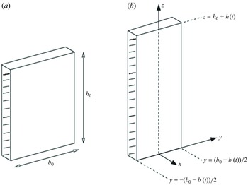


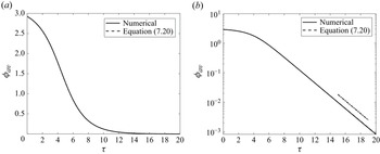


 Open access