3.1. Eddy thermal diffusivity model

Integrating (2.5) with respect to $x$ , one obtains

(3.1) \begin{equation} \overline {u'T'} - \kappa \frac {{\rm d}\overline {T}}{{\rm d}x} = - \kappa \frac {{\rm d} \overline {T}}{{\rm d}x} \bigg |_{x=0} = \kappa {\textit{Nu}} \frac {\varDelta T}{H} ,\end{equation}

where ${\textit{Nu}}$ , being the ratio of the actual heat flux normal to the walls to the heat flux when there is only thermal conduction, is defined by

(3.2) \begin{equation} {\textit{Nu}} \equiv \frac {\overline { u' T'} - \kappa {\rm d}\overline {T} /{\rm d}x}{\kappa \varDelta T/H} \equiv \frac {q}{\kappa \varDelta T/H} .\end{equation}

The heat flux is given by the product of $q$ and $\rho c$ , where $c$ is the specific heat capacity of the fluid. We introduce a space-dependent function $K(x)$ for the eddy thermal diffusivity

(3.3) \begin{equation} \overline {u'T'} \equiv - K(x) \frac {{\rm d}\overline {T}}{{\rm d}x} .\end{equation}

Then (3.1) with (3.3) can be integrated to give (Ruckenstein & Felske Reference Ruckenstein and Felske1980)

(3.4) \begin{equation} \frac {1}{\varDelta T} [\overline {T}(x)-T_m]= \frac {1}{2} - {\textit{Nu}} \int _0^{x/H} \frac {{\rm d}y}{1+K(yH)/\kappa } , \end{equation}

and ${\textit{Nu}}$ is obtained by using the boundary condition at $x=H/2$ in (2.7)

(3.5) \begin{equation} {\textit{Nu}} = \frac {1}{2} \left [ \int _0^{1/2} \frac {{\rm d}y}{1+K(yH)/\kappa } \right ]^{-1} .\end{equation}

Thus, both $\overline {T}$ and ${\textit{Nu}}$ can be determined if $K(x)$ is known.

The characteristic temperature scales in the inner region near the wall and the outer region near the centreline between the two walls should have different dependencies on $\nu$ and $\kappa$ as molecular diffusivities are expected to play a significant role in the inner region but not the outer region. As seen from (3.4), this suggests that the eddy diffusivity $K(x)$ is governed by two independent parameters in the inner and outer regions. Thus, we model $K(x)$ separately in the inner and outer regions and in the intermediate region between them. Due to the no-slip and isothermal boundary conditions at the two vertical sidewalls, $u'$ , $T'$ and $\partial u'/\partial x=-(\partial v'/\partial y+ \partial w'/\partial z)$ vanish at $x=0$ , and this leads to the vanishing of $\overline {u'T'}$ and its first- and second-order derivatives with respect to $x$ at $x=0$ (Ruckenstein & Felske Reference Ruckenstein and Felske1980; Ching Reference Ching2023). Since the temperature gradient at $x=0$ , being proportional to ${\textit{Nu}}$ , is non-zero, $K(x)$ and its first- and second-order derivatives should also vanish at $x=0$ . Thus, we model $K(x)/\nu$ by a cubic function in the inner region. In the outer region, we make use of the symmetry of the problem. Since $\overline {u'T'}$ is symmetric and $\overline {T}$ is antisymmetric about the centreline $x=H/2$ , $K(x)$ is symmetric about $x=H/2$ and attains a maximum value at $x=H/2$ . This motivates us to model $K(x)/\nu$ by the simplest symmetric quadratic function with a peak at $x=H/2$ in the outer region. For the intermediate region, we choose a linear function that connects continuously to the other two regions as it is simple and the resulting $K(x)$ gives rise to a ${\textit{Nu}}$ that scales as ${\textit{Ra}}^{1/3}$ in the high-Ra limit in accord with the theoretical result (Ching Reference Ching2023) (cf. § 4). Putting all these results together, we propose a three-layer model for $K(x)/\nu$

(3.6) \begin{eqnarray} \frac {K(x)}{\nu } = \begin{cases} A y^3, & 0 \le y \le y_1 ,\\ c_1 + c_2 y, & y_1 \lt y \lt y_2, \\ C_m[1- b(1/2-y)^2], & y_2 \le y \le 1/2, \end{cases} \end{eqnarray}

where $y=x/H$ . Near the walls, the turbulent heat flux is expected to be small compared with the conductive heat flux, or equivalently, $K(x)$ is expected to be small compared with  $\kappa$ . Thus, a natural characteristic length scale for the inner region is given by

(3.7) \begin{equation} l_i = \frac {H}{(\textit{Pr} A)^{1/3}} , \end{equation}

which is the position at which our proposed model of eddy thermal diffusivity is equal to $\kappa$ , and we set the width of the inner region to be $2 l_i$ , i.e. $y_1 H= 2 l_i$ . We note that the equality of the eddy and molecular thermal diffusivities was used to define the thickness of the thermal boundary layer in vertical convection by Howland et al. (Reference Howland, Ng, Verzicco and Lohse2022). We fix the width of the outer region to be $0.2 H$ with $y_2=0.3$ and take $b=4$ . These values are guided by the DNS data (Howland et al. Reference Howland, Ng, Verzicco and Lohse2022). The constants $c_1$ and $c_2$ are fixed by the continuity of $K(x)/\nu$ at $x=y_1H$ and $x=y_2H$

(3.8) \begin{align} c_1 = \frac {Ay_1^3 y_2-C_m\left [1-b(1/2-y_2)^2\right ]y_1}{y_2-y_1}, \quad c_2 = \frac {C_m\left [1-b(1/2-y_2)^2\right ]- Ay_1^3}{y_2-y_1} .\end{align}

Hence, the model has two independent parameters: $A$ and $C_m$ . We will show below that they determine the characteristic velocities for heat transfer in the inner and outer regions, respectively.

3.2. Mean temperature profiles

Substituting (3.6) into (3.4) and evaluating the integral, we obtain $\overline {T}(x)$

(3.9) \begin{align} \frac {1}{\varDelta T} [T_h - \overline {T}(yH)] &=\begin{cases} {\textit{Nu}} \ I_1(y), \qquad 0 \le y \le y_1 , \\ {\textit{Nu}} \ [I_1(y_1)+I_2(y)], & y_1 \lt y \lt y_2,\end{cases} \\[-12pt] \nonumber \end{align}

(3.10) \begin{align} \frac {1}{\varDelta T} [\overline {T}(yH)-T_{m}] &= {\textit{Nu}} \ I_3(y), \qquad y_2 \le y \le 1/2 , \\[9pt] \nonumber \end{align}

where

(3.11) \begin{equation} {\textit{Nu}} = \frac {1}{2[I_1(y_1)+ I_2(y_2) + I_3(y_2)]} , \end{equation}

and

(3.12) \begin{align} \nonumber I_1(y) &\equiv \frac {1}{\textit{Pr}^{\frac {1}{3}} {A^{\frac {1}{3}}}} \int _0^{\textit{Pr}^{1/3} A^{1/3}y} \frac {{\rm d}y' }{1+ y'^3} = \frac {1}{3\textit{Pr}^{\frac {1}{3}} A^{\frac {1}{3}}} \left \{ \frac {1}{2} \log \left [\frac {\left(1+\textit{Pr}^{\frac {1}{3}} A^{\frac {1}{3}} y\right)^3}{1+\textit{Pr} A y^3}\right ] \right . \nonumber \\& \quad +\left . \sqrt {3}\arctan \left (\frac {2 {\textit{Pr}^{\frac {1}{3}}} A^{\frac {1}{3}} y -1}{\sqrt {3}} \right ) + \frac {\sqrt {3} \pi }{6} \right \}\! , \end{align}

(3.13) \begin{align} I_2(y) &\equiv \int _{y_1}^{y} \frac {{\rm d}y' }{1+ \textit{Pr}(c_1 + c_2 y')} = \frac {1}{\textit{Pr} c_2} \log \left [ \frac {1+\textit{Pr}(c_1+ c_2y)}{1+\textit{Pr}(c_1 + c_2 y_1)} \right ]\! , \end{align}

(3.14) \begin{align} I_3 (y) &\equiv \int _{y}^{1/2} \frac {{\rm d}y' }{1+ {\textit{Pr}} C_m[1- b(1/2-y')^2]} \nonumber \\&= \frac {1}{2B(1+C_m {\textit{Pr}})} \log \left | \frac {1 + B (1/2-y)}{1 - B (1/2-y)} \right | , \ B= \sqrt {b C_m {\textit{Pr}}/(1+C_m {\textit{Pr}})}. \end{align}

We focus on the mean temperature profile in the inner and outer regions. The analytical results (3.9) and (3.10) reveal that $\overline {T}(x)$ is given by two universal scaling functions of their respective characteristic temperature and length scales in these two regions, namely

(3.15) \begin{align} T_h - \overline {T}(x) &= T_i F_i (x/l_i) \qquad \mbox{inner wall region} ,\end{align}

(3.16) \begin{align} \overline {T}(x) - T_m &= T_o F_o(x/H) \qquad \mbox{outer centreline region} , \end{align}

where the inner and outer scaling functions are

(3.17) \begin{align} F_i(z) &= \frac {1}{6}\log \left [\frac {(1+z)^3}{1+z^3}\right ] + \frac {\sqrt {3}}{3} \arctan \left ( \frac {2z -1}{\sqrt {3}}\right ) + \frac {\sqrt {3}\pi }{18} , \end{align}

(3.18) \begin{align} F_o(z) &= \frac {1}{2\sqrt {b}} \log \left | \frac {1+\sqrt {b}(1/2-z)}{1-\sqrt {b}(1/2-z)} \right | = \frac {1}{4} \log \left (\frac {1 -z}{z}\right )\!, \end{align}

the inner and outer temperature scales are

(3.19) \begin{align} T_i &= \frac {\varDelta T Nu}{(\textit{Pr} A)^{1/3}} , \end{align}

(3.20) \begin{align} T_o &= \frac {\varDelta T \textit{Nu}}{\textit{Pr} C_m} , \end{align}

and the characteristic length scales in the inner and outer regions are $l_i$ and $H$ , respectively. To obtain (3.16) with (3.18), we have used the approximation ${\textit{Pr}} C_m \gg 1$ , which follows from the dominance of the turbulent heat flux over the conductive heat flux, $|\overline {u'T'}| \gg \kappa |{\rm d} \overline {T}/{\rm d}x|$ , at $x=H/2$ in the outer region for turbulent convective flows. Using (3.2) and (3.7), we can rewrite (3.19) and (3.20) as

(3.21) \begin{equation} V_i T_i = V_o T_o = q ,\end{equation}

where

(3.22) \begin{align} V_i &\equiv \frac {\kappa }{l_i} = \frac {\kappa }{H} (\textit{Pr} A)^{1/3} , \end{align}

(3.23) \begin{align} V_o &\equiv \frac {K(H/2)}{H} = \frac {\nu C_m}{H} . \end{align}

Thus, the two parameters $A$ and $C_m$ determine $V_i$ and $V_o$ , the characteristic velocities for heat transfer in the inner and outer regions, respectively.

4.1. Validation

Using DNS data for ${\textit{Pr}}=1, 2, 5, 10$ and $100$ and ${\textit{Ra}}$ ranging from $10^{6}$ to $10^{9}$ (Howland et al. Reference Howland, Ng, Verzicco and Lohse2022), we evaluate $K(x)/\nu$ , we fit it by $A (x/H)^3$ in the region $0 \le x/H \le 2 l_i/H=2/(\textit{Pr} A)^{1/3}$ using the least-square method to obtain $A$ and extract $C_m$ directly as $C_m=K(H/2)/\nu$ . The values of $A$ and $C_m$ are shown in table 1. In determining $\overline {T}(x)$ and ${\textit{Nu}}$ , the relevant quantity is $F(x) = 1/[1+ Pr K(x)/\nu ]$ (see (3.4) and (3.5)). We compare $F(x)$ evaluated using the eddy diffusivity model (3.6) and the DNS data in figure 1. Good agreement can be seen, which is further supported by the relatively small errors of the values of ${\textit{Nu}}$ estimated using the model with respect to the DNS data (see table 1). Good agreement between the analytical result for $\overline {T}$ and the DNS data is also shown in figure 1. If $K(x)/\nu$ is modelled by $A(x/H)^3$ throughout the whole region (Ruckenstein & Felske Reference Ruckenstein and Felske1980), the estimated ${\textit{Nu}}$ would be given by $1/[2 I_1(1/2)]$ . As shown in table 1, the relative errors of these estimates of ${\textit{Nu}}$ are substantially larger for ${\textit{Pr}} \le 5$ .

Table 1.

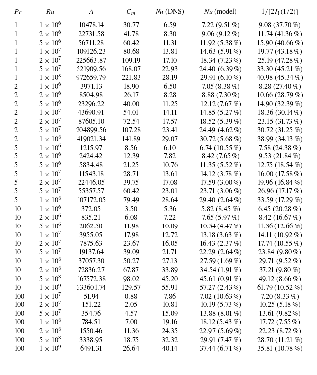
Values of the parameters $A$ and $C_m$ of the eddy thermal diffusivity model. Here, ${\textit{Nu}}$ (model) are the  ${\textit{Nu}}$ values estimated using the eddy diffusivity model with these values of $A$ and $C_m$ and $1/[I_1(1/2)]$ are the values of ${\textit{Nu}}$ obtained when $K(x)/\nu$ is modelled instead by $A(x/H)^3$ . The numbers in parentheses are the relative errors of the estimated values of ${\textit{Nu}}$ with respect to the DNS data by Howland et al. (Reference Howland, Ng, Verzicco and Lohse2022).

Figure 1.

Value of $F(x) = 1/[1+Pr K(x)/\nu ]$ vs $x$ at ${\textit{Ra}}=10^8$ for ${\textit{Pr}}=1$ (black), ${\textit{Pr}}=10$ (blue) and ${\textit{Pr}}=100$ (green). The symbols are DNS data (Howland et al. Reference Howland, Ng, Verzicco and Lohse2022) and the solid lines are evaluated using the eddy diffusivity model (3.6) with the values of $A$ and $C_m$ from table 1. In the inset, we compare the analytical result of the mean temperature profiles $\overline {T}(x)$ from the model (solid lines) with the DNS data. The dashed lines denote the positions of $y_1$ and $y_2=0.3$ .

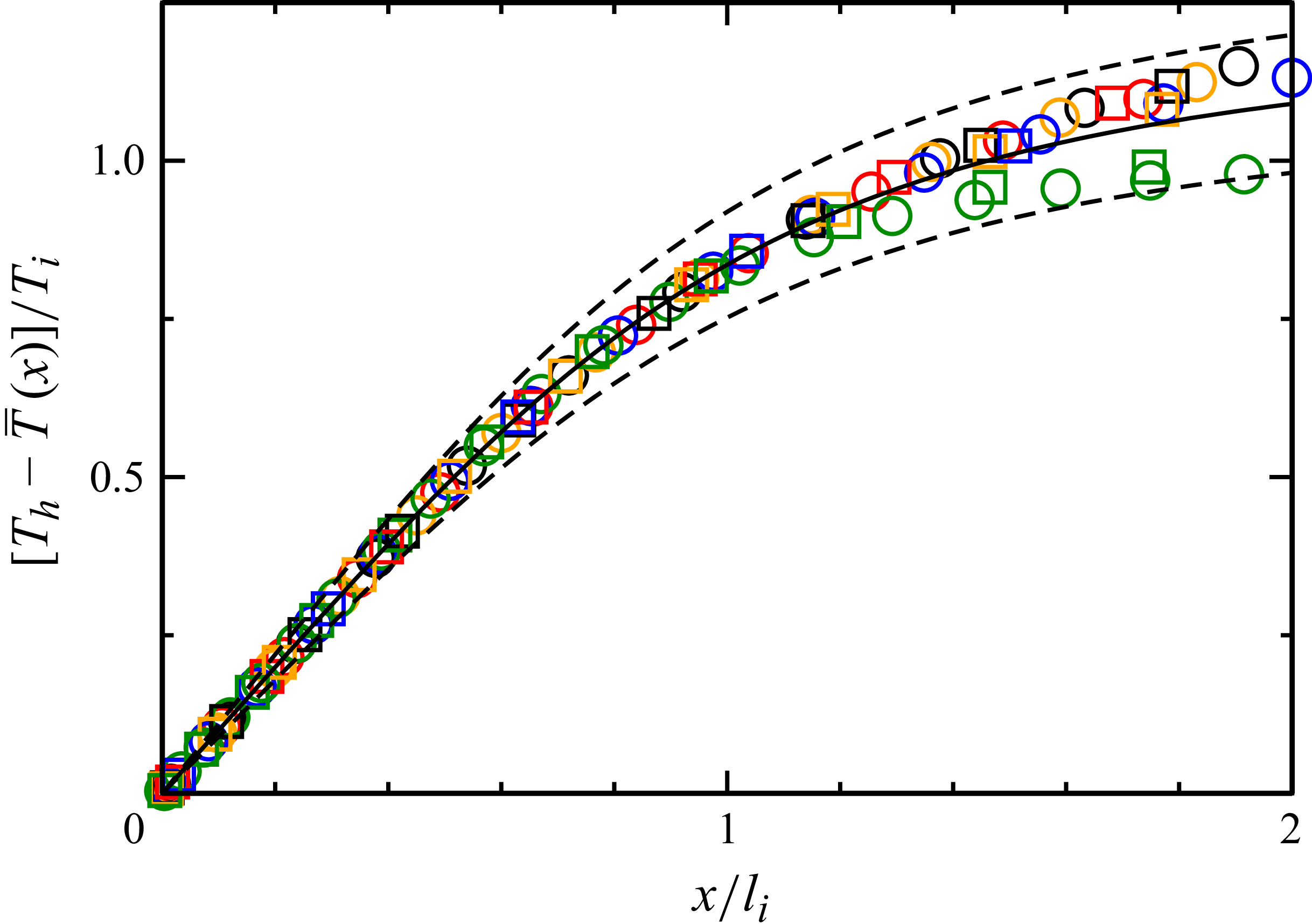
In figure 2, we plot $(T_h-\overline {T} )/T_i$ as a function of $x/l_i$ . The DNS data for different ${\textit{Pr}}$ and ${\textit{Ra}}$ collapse onto a single curve that is well described by the theoretical inner scaling function $F_i$ in (3.17) for $0 \le x/l_i \lt 2$ , validating (3.15). In this region, $F_i$ clearly deviates from a linear function, showing that the turbulent heat flux $\overline {u'T'}$ cannot be neglected even within the inner region. Following George & Capp (Reference George and Capp1979), we express the temperature and length scales in the inner region in terms of heat flux, or equivalently, $q$ , the buoyancy parameter $\alpha g$ and the molecular diffusivities $\nu$ and $\kappa$ . Dimensional analysis then yields

(4.1) \begin{eqnarray} T_i = \left ( \frac {q^3}{\alpha g \kappa } \right )^{\!\frac {1}{4}} g_i(\textit{Pr}) = T_{i,\textit{GC}} g_i(\textit{Pr}) = \varDelta T \textit{Nu}^{3/4} (\textit{Ra} \textit{Pr})^{-\frac {1}{4}} g_i(\textit{Pr}) ,\end{eqnarray}

up to some ${\textit{Pr}}$ -dependent function $g_i(\textit{Pr})$ . Using (3.21) and (3.22), we have

(4.2) \begin{equation} l_i = \left ( \frac {\kappa ^3}{\alpha g q}\right )^{\!\frac {1}{4}} g_i(\textit{Pr}) = l_{i,\textit{GC}} g_i(\textit{Pr}) .\end{equation}

Figure 2.

Value of $(T_h-\overline {T})/T_i$ vs $x/l_i$ at ${\textit{Ra}}_{\textit{min}}$ (circles) and ${\textit{Ra}}_{\textit{max}}$ (squares) for ${\textit{Pr}}=1$ (black), ${\textit{Pr}}=2$ (red), ${\textit{Pr}}=5$ (orange), ${\textit{Pr}}=10$ (blue) and ${\textit{Pr}}=100$ (green). Here, ${\textit{Ra}}_{\textit{min}}$ and ${\textit{Ra}}_{\textit{max}}$ are the minimum and maximum values of ${\textit{Ra}}$ for the corresponding ${\textit{Pr}}$ (see table 1). The solid line is the inner scaling function $F_i$ given by (3.17) and the two dashed lines indicate $0.9F_i$ and $1.1F_i$ .

Our inner temperature and length scales $T_i$ and $l_i$ thus differ from the scales $T_{i,\textit{GC}} = (q^3/\alpha g \kappa )^{1/4}$ and $l_{i,\textit{GC}}=(\kappa ^3/\alpha g q)^{1/4}$ adopted by George & Capp (Reference George and Capp1979). The inclusion of $\nu$ in our analysis leads to an additional function $g_i(\textit{Pr})$ , and this enables us to obtain a universal scaling function $F_i$ in the inner region for all ${\textit{Pr}}$ . By comparing (3.19) with (4.1), we obtain

(4.3) \begin{eqnarray} (\textit{Pr} A)^{-1/3} = (\textit{Ra} \textit{Pr} \textit{Nu})^{-1/4} g_i(\textit{Pr}) ,\end{eqnarray}

which is used to evaluate $g_i(\textit{Pr})$ . We find that $g_i(\textit{Pr})$ can be fitted by a power law $k_i \textit{Pr}^{\beta }$ with $\beta = 0.425 \approx 3/7$ and $k_i = 2.18$ . A commonly used velocity scale in the inner region is the friction velocity $u_\tau = \sqrt {\nu{\rm d}\overline {w}/{\rm d}x |_{x=0}}$ . It is interesting to compare the inner velocity scale $V_i$ and $u_\tau$ . Using (3.22) and (4.3), we obtain

(4.4) \begin{equation} \frac {V_i}{u_\tau } =\frac {(\textit{Ra} \textit{Nu})^{1/4} }{g_i(\textit{Pr}) \textit{Pr}^{3/4} Re_\tau } ,\end{equation}

where ${\textit{Re}}_\tau =u_\tau H/\nu$ is the shear Reynolds number. The theoretical results of Ching (Reference Ching2023) that ${\textit{Nu}}$ and ${\textit{Re}}_\tau$ scale as ${\textit{Ra}}^{1/3}$ in the high- ${\textit{Ra}}$ limit then imply that $V_i$ is related to $u_\tau$ by a ${\textit{Pr}}$ -dependent function $h(\textit{Pr})$ when ${\textit{Ra}}$ is sufficiently large

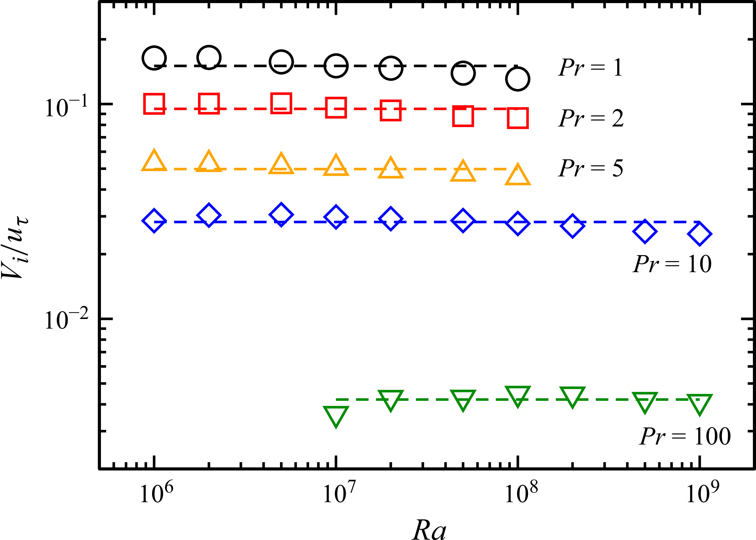
(4.5) \begin{equation} V_i \approx h(\textit{Pr}) u_\tau .\end{equation}

It can be seen in figure 3 that (4.5) is confirmed and $h(\textit{Pr})$ is a decreasing function of ${\textit{Pr}}$ . As a result, if the mean temperature profiles are rescaled by $l_\tau \equiv \kappa /u_\tau$ and $T_\tau \equiv q/u_\tau$ instead of $l_i$ and $T_i$ , the profiles for different ${\textit{Pr}}$ do not collapse beyond the linear region near the wall (as shown in figure 5b of Howland et al. Reference Howland, Ng, Verzicco and Lohse2022).

Figure 3.

Value of $V_i/u_\tau$ as a function of ${\textit{Ra}}$ . The dashed lines give the average values of $V_i/u_\tau$ over ${\textit{Ra}}$ for each ${\textit{Pr}}$ .

Next we check (3.16). As shown in figure 4, the rescaling of $\overline {T}-T_m$ by $T_o$ results in an approximate collapse of the data in the region $0.3 \le x/H \le 0.5$ . The collapsed data are consistent with the outer scaling function $F_o$ with $b=4$ in (3.18). These observations support our choice of $y_2=0.3$ and $b=4$ and validate our proposed functional form of $K(x)$ in the outer region. If the outer temperature scale $T_{o,\textit{GC}}$ proposed by George & Capp (Reference George and Capp1979) is used instead of $T_o$ , the data collapse is worse (see the inset of figure 4). The scale $T_{o,\textit{GC}}$ , given by

(4.6) \begin{equation} T_{o,\textit{GC}}=\left (\frac {q^2}{\alpha g H} \right )^{1/3} , \end{equation}

was obtained by assuming that the temperature scale in the outer region depends on $q$ , $\alpha g$ and $H$ only and not on the molecular diffusivities $\nu$ and $\kappa$ . We find that

(4.7) \begin{equation} C_m \to k_o (\textit{Ra} \textit{Nu})^{1/3} \textit{Pr}^{-2/3} ,\end{equation}

with $k_o = 0.162$ for sufficiently large ${\textit{Ra}}$ . This implies that $T_o \to k_o^{-1} T_{o,\textit{GC}}$ when ${\textit{Ra}}$ is greater than certain threshold value ${\textit{Ra}}_c(\textit{Pr})$ and ${\textit{Ra}}_c(\textit{Pr})$ increases with ${\textit{Pr}}$ .

Figure 4.

Plot of $(\overline {T} - T_m)/T_o$ vs $x/H$ at ${\textit{Ra}}_{\textit{min}}$ and ${\textit{Ra}}_{\textit{max}}$ for ${\textit{Pr}}=1, 2, 5, 10, 100$ . Same symbols as in figure 2. The solid line is the function $F_o$ given by (3.18). A similar plot is shown in the inset with the temperature rescaled by $T_{o,\textit{GC}}$ instead of $T_o$ .

Finally, we show that our model gives ${\textit{Nu}} \sim \textit{Ra}^{1/3}$ in the high- ${\textit{Ra}}$ limit. Using (4.3) and (4.7), it can be shown that, for sufficiently large ${\textit{Ra}}$ , $I_1(y_1) \sim (Ra Nu)^{-1/4}$ , $I_2(y_2) \sim (Ra Nu)^{-1/3} \ln (Ra Nu)$ and $I_3(y_2) \sim (Ra Nu)^{-1/3}$ and hence

(4.8) \begin{eqnarray} {\textit{Nu}} \approx \frac {1}{2I_1(y_1)} \Rightarrow {\textit{Nu}} \sim \textit{Ra}^{1/3} . \end{eqnarray}

Substituting the theoretical result of ${\textit{Nu}} \approx [C^2f(\textit{Pr})]^{1/3}\textit{Pr}^{-1/9} \textit{Ra}^{1/3} = \gamma (\textit{Pr}) \textit{Ra}^{1/3}$ for ${\textit{Pr}} \ge 1$ in the high- ${\textit{Ra}}$ limit (Ching Reference Ching2023) into (4.3) and (4.7), we obtain

(4.9) \begin{align} A &\approx [\gamma (\textit{Pr})]^{3/4} [g_i(\textit{Pr})]^{-3} \textit{Pr}^{-1/4} \textit{Ra} = C_1(\textit{Pr}) \textit{Ra} ,\end{align}

(4.10) \begin{align} C_m &\approx k_o [\gamma (\textit{Pr})]^{1/3} \textit{Pr}^{-2/3} \textit{Ra}^{4/9} = C_2(\textit{Pr}) \textit{Ra}^{4/9} , \end{align}

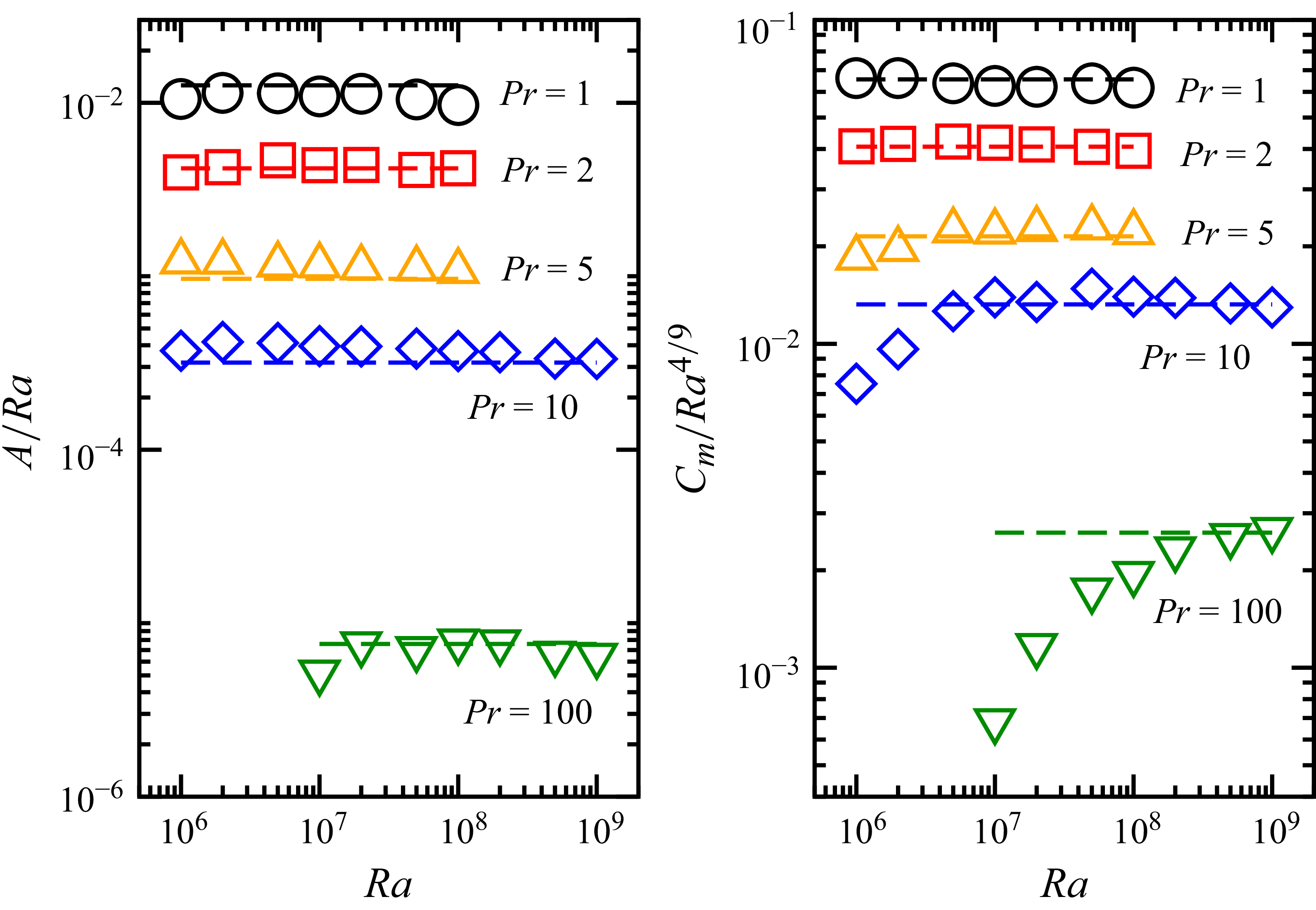
when ${\textit{Ra}}$ is sufficiently large. Such ${\textit{Ra}}$ -dependencies of $A$ and $C_m$ are confirmed in figure 5.

Figure 5.

Plot of $A/Ra$ and $C_m/\textit{Ra}^{4/9}$ vs ${\textit{Ra}}$ .The dashed lines for different ${\textit{Pr}}$ are the values of $C_1(\textit{Pr})$ and $C_2(\textit{Pr})$ obtained by using $C=0.043$ , $f(\textit{Pr})\approx 0.19$ (Ching Reference Ching2023) and the fitted values of $k_i$ , $\beta$ and $k_o$ (see (4.9) and (4.10)).

4.2. Comparison with mean temperature profiles reported in previous studies

One often-cited result for the mean temperature profile was obtained by George & Capp (Reference George and Capp1979). They proposed scaling functions in terms of $T_{i,\textit{GC}}$ and $l_{i,\textit{GC}}$ in the inner region and $T_{o,\textit{GC}}$ and $H$ in the outer region. In an overlap layer in which both scaling functions hold, they obtained

(4.11) \begin{align} \frac {T_h - \overline {T}(x)}{T_{i,\textit{GC}}} &= - K_1 \left (\frac {x}{l_{i,\textit{GC}}}\right )^{-1/3} + \phi _1(\textit{Pr}) , \end{align}

(4.12) \begin{align} \frac {\overline {T}(x)-T_m}{T_{o,\textit{GC}}} &= K_1 \left (\frac {x}{H}\right )^{-1/3} + \theta _1 , \end{align}

with undetermined constants $K_1$ , $\phi _1(\textit{Pr})$ and $\theta _1$ ; the independence of $K_1$ and $\theta _1$ from ${\textit{Pr}}$ follows from the independence of the outer scaling function from $\nu$ or $\kappa$ . Fitting their DNS data for ${\textit{Pr}}=0.709$ (air), Versteegh & Nieuwstadt (Reference Versteegh and Nieuwstadt1999) and Ng et al. (Reference Ng, Chung and Ooi2013) found $K_1=4.2$ . Using the DNS data of Howland et al. (Reference Howland, Ng, Verzicco and Lohse2022), we find that the region that (4.11) with $K_1=4.2$ can fit decreases drastically for larger ${\textit{Pr}}$ while our result for the inner region (3.15) with (3.17), rewritten as

(4.13) \begin{eqnarray} \frac {T_h - \overline {T}(x)}{T_{i,\textit{GC}}} = g_i(\textit{Pr}) F_i \left (\frac {1}{g_i(\textit{Pr})}\frac {x}{l_{i,\textit{GC}}}\right ) , \end{eqnarray}

can give good fits for all the 5 values of ${\textit{Pr}}$ studied. The comparison for ${\textit{Pr}}=1$ and ${\textit{Pr}}=100$ is shown in figure 6.

Figure 6.

Plots of $[T_h - \overline {T}(x)]/T_{i,\textit{GC}}$ vs $x/l_{i,\textit{GC}}$ for ${\textit{Pr}}=1$ (left panel) and ${\textit{Pr}}=100$ (right panel) at ${\textit{Ra}} = 10^6$ (plusses), $2\times 10^6$ (crosses), $5\times 10^6$ (stars), $10^7$ (circles), $2\times 10^7$ (squares), $5\times 10^7$ (diamonds), $10^8$ (triangles), $2\times 10^8$ (left triangles), $5\times 10^8$ (inverted triangles) and $10^9$ (right triangles). The red solid lines are (4.13) and the blue dashed lines are (4.11) with $K_1=4.2$ , $\phi _1(1)=5.10$ and $\phi _1(100)=5.15$ .

Using the same approach but with the temperature scale $T_{i,\textit{GC}}$ for both the inner and outer regions, Hölling & Herwig (Reference Hölling and Herwig2005) obtained a logarithmic profile in the overlap layer

(4.14) \begin{align} \frac {T_h - \overline {T}(x)}{T_{i,\textit{GC}}} &= K_2 \log \left (\frac {x}{l_{i,\textit{GC}}}\right ) + \phi _2(\textit{Pr}) , \end{align}

(4.15) \begin{align} \frac {\overline {T}(x)-T_m}{T_{i,\textit{GC}}} &= - K_2 \log \left (\frac {x}{H}\right ) + \theta _2 , \end{align}

with undetermined constants $K_2$ , $\phi _2(\textit{Pr})$ and $\theta _2$ . Different values of $K_2$ and $\phi _2$ , obtained by fitting DNS data for air, were reported (Versteegh & Nieuwstadt Reference Versteegh and Nieuwstadt1999; Hölling & Herwig Reference Hölling and Herwig2005; Kiš & Herwig Reference Kiš and Herwig2012; Ng et al. Reference Ng, Chung and Ooi2013). We thus test instead the relation between ${\textit{Nu}}$ , ${\textit{Ra}}$ and ${\textit{Pr}}$ , obtained by adding (4.14) and (4.15) and using (4.1) and (4.2)

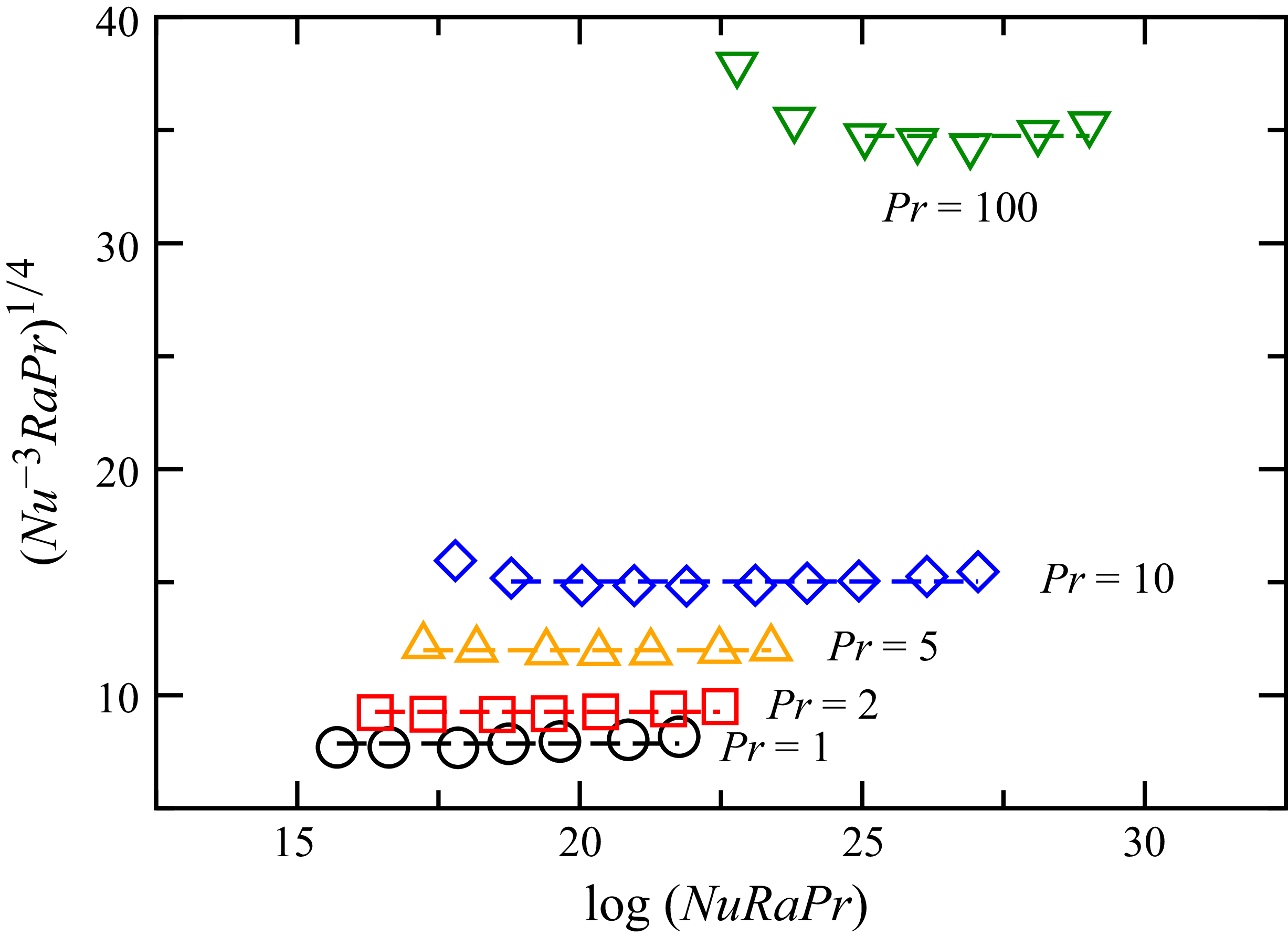
(4.16) \begin{align} (\textit{Nu}^{-3} \textit{Ra} \textit{Pr})^{1/4} = \frac {K_2}{2} \log (\textit{Nu} \textit{Ra} \textit{Pr}) + 2[\phi _2(\textit{Pr})+\theta _2] .\end{align}

Balaji, Hölling & Herwig (Reference Balaji, Hölling and Herwig2007) assumed (4.14) to hold up to $x=H/2$ and obtained a different relation than (4.16). As shown in figure 7, the DNS data (Howland et al. Reference Howland, Ng, Verzicco and Lohse2022) are consistent with (4.16) with $K_2=0$ , indicating their incompatibility with (4.14) and (4.15). When $K_2=0$ , (4.16) reduces to ${\textit{Nu}} \sim \textit{Ra}^{1/3}$ .

Figure 7.

Plot of $(\textit{Nu}^{-3} \textit{Ra} Pr)^{1/4}$ vs $\log (Nu \textit{Ra} Pr)$ using DNS data of Howland et al. (Reference Howland, Ng, Verzicco and Lohse2022). The dashed lines for different ${\textit{Pr}}$ are the best fits of (4.16) with $K_2=0$ .

A recent work (Li et al. Reference Li, Jia, Liu, Jiao and Zhang2023) studied the mean velocity and temperature profiles by modelling the Reynolds stress and turbulent heat flux

(4.17) \begin{align} \overline {u'w'} &= -k_1 x^2 \left ( \frac {\partial \overline {w}}{\partial x} \right )^2 \!,\end{align}

(4.18) \begin{align} \overline {u'T'} &= -k_2 x^2 \frac {\partial \overline {w}}{\partial x} \frac {\partial \overline {T}}{\partial x} ,\end{align}

where $k_1$ and $k_2$ are dimensionless coefficients. As discussed in § 3.1, $\overline {u'T'}$ and its first- and second-order derivatives with respect to $x$ vanish at $x=0$ due to the boundary conditions. Similar arguments require $\overline {u'w'}$ and its first- and second-order derivatives with respect to $x$ to vanish at $x=0$ . These properties should be satisfied by any closure model but they are violated by (4.17) and (4.18). Since both the mean velocity and temperature gradients, $\partial \overline {w}/\partial x$ and $\partial \overline {T}/\partial x$ , are non-zero at $x=0$ , the model expressions on the right-hand side of (4.17) and (4.18) have non-vanishing second-order derivatives at $x=0$ . Applying (4.17) and (4.18) to the near-centreline outer region, Li et al., obtained an inverse cubic-root dependence for the mean temperature profile ((2.14b) of Li et al. Reference Li, Jia, Liu, Jiao and Zhang2023), which we rewrite as

(4.19) \begin{equation} \frac {\overline {T}(x)-T_m}{T_\tau } = c K\left [ \left (\frac {x}{H} \right )^{-1/3} - 2^{1/3} \right ] =c K x^* ,\end{equation}

where $K = (\alpha g H T_\tau /u_\tau ^2)^{1/3}$ , $c \approx 3.8$ and

(4.20) \begin{equation} x^*\equiv \left (\frac {x}{H} \right )^{-1/3} - 2^{1/3} .\end{equation}

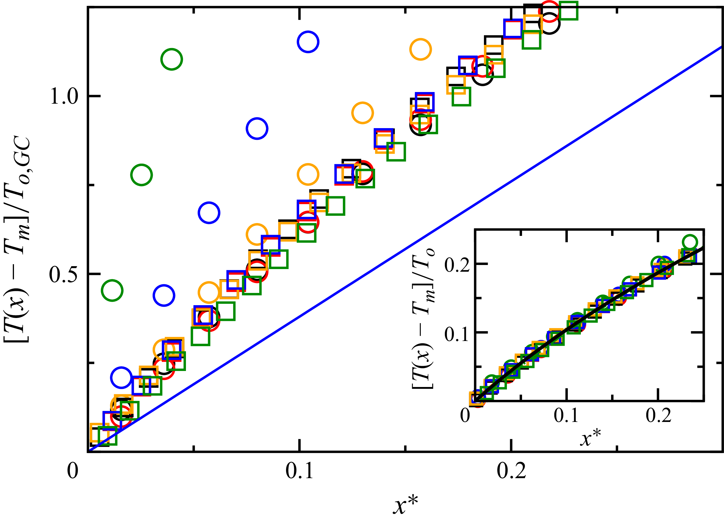
We note that (4.19) implies that the mean temperature profiles in the outer region would collapse onto a straight line in $x^*$ when temperature is rescaled by $T_\tau /K=T_{o,\textit{GC}}$ . Using (4.20), we rewrite our result for the outer region, (3.16) with (3.18), in terms of $x^*$

(4.21) \begin{equation} \frac {\overline {T}(x)-T_m}{T_o} = \frac {1}{4} \log \left[\left(x^*+2^{1/3}\right)^3 - 1\right]\! .\end{equation}

In figure 8, it can be clearly seen that the mean temperature profiles in the outer region do not collapse onto the straight line $c x^*$ when rescaled by $T_{o,\textit{GC}}$ , contrary to the prediction by (4.19), but they are well represented by (4.21).

Figure 8.

Plot of $(\overline {T} - T_m)/(T_{o,\textit{GC}})$ vs $x^*$ at ${\textit{Ra}}_{\textit{min}}$ and ${\textit{Ra}}_{\textit{max}}$ for ${\textit{Pr}}=1, 2, 5, 10, 100$ . Same symbols as in figure 2 and the solid straight line is $c x^*$ . In the inset, a similar plot is shown with the temperature rescaled by $T_{o}$ instead of $T_{o,\textit{GC}}$ and the solid line is (4.21).