2. Drift kinetic equation for ions in a generic stellarator

We assume $a \sim R$ in this section, but we keep the distinction between $a$ and $R$ in our estimates in preparation for the expansion in small inverse aspect ratio in §§ 3, 4, 5 and 8.

We assume that the magnetic field $\boldsymbol {B}$ is constant in time and hence the electric field $\boldsymbol {E}$ satisfies $\boldsymbol {E}(\boldsymbol {x}, t) = - \boldsymbol {\nabla } \phi (\boldsymbol {x}, t)$. The electric potential $\phi$ is of order $T_i/e$, has a characteristic length scale of the order of the minor radius $a$, and is determined by the quasineutrality equation

(2.1)\begin{equation} Z_i \int f_i (\boldsymbol{x}, \boldsymbol{v}, t) \, \mathrm{d}^{3} v = \int f_{e} (\boldsymbol{x}, \boldsymbol{v}, t) \, \mathrm{d}^{3} v, \end{equation}

where $f_i (\boldsymbol {x}, \boldsymbol {v}, t)$ and $f_e(\boldsymbol {x}, \boldsymbol {v}, t)$ are the distribution functions of ions and electrons, $\boldsymbol {x}$ and $\boldsymbol {v}$ are the particle's Cartesian position and velocity, and $t$ is time. Throughout the paper, we assume that the electrons can be modelled with the modified Maxwell–Boltzmann response

(2.2)\begin{equation} \int f_e (\boldsymbol{x}, \boldsymbol{v}, t) \, \mathrm{d}^{3} v = \hat{n}_e(r(\boldsymbol{x}), t)\exp\left(\frac{e\phi(\boldsymbol{x}, t)}{T_e (r(\boldsymbol{x}), t)}\right), \end{equation}

where $T_e (r, t)$ is the temperature of the electrons and $\hat {n}_e(r, t)$ is the density of electrons in the absence of $\phi$. Note that $\hat {n}_e$ and $T_e$ are flux functions that only depend on the flux surface label $r(\boldsymbol {x})$. We define $r$ more carefully below.

We use the drift kinetic equation (Hazeltine Reference Hazeltine1973) to obtain the ion distribution function. To describe velocity space, we choose the coordinates $\{ \mathcal {E}, \mu, \sigma, \varphi \}$, where $\mathcal {E} :=v^{2}/2 +Z_i e \phi /m_i$ is the total energy per unit mass, $\mu :=v_\perp ^{2} /2B$ is the magnetic moment, $\sigma$ is the sign of the parallel velocity and $\varphi$ is the gyrophase, defined such that

(2.3)\begin{equation} \frac{\boldsymbol{v}_\perp}{v_\perp} = \hat{\boldsymbol{e}}_\perp (\boldsymbol{x}, \varphi) := \cos \varphi\, \hat{\boldsymbol{e}}_1 (\boldsymbol{x}) + \sin \varphi \, \hat{\boldsymbol{e}}_2 (\boldsymbol{x}). \end{equation}

Here, $\boldsymbol {v}_\perp$ is the component of $\boldsymbol {v}$ perpendicular to the magnetic field, $v_\perp := |\boldsymbol {v}_\perp |$ and $\hat {\boldsymbol {e}}_1(\boldsymbol {x})$ and $\hat {\boldsymbol {e}}_2(\boldsymbol {x})$ are two unit vectors that form an orthonormal basis with the unit vector parallel to the magnetic field $\hat {\boldsymbol {b}}(\boldsymbol {x}) = \boldsymbol {B}/B$ and satisfy $\hat {\boldsymbol {e}}_1 \times \hat {\boldsymbol {e}}_2 = \hat {\boldsymbol {b}}$. In the coordinates $\{ \mathcal {E}, \mu, \sigma, \varphi \}$, the velocity-space volume element is

(2.4)\begin{equation} \mathrm{d}^{3} v = \frac{\mathrm{d} \mathcal{E}\, \mathrm{d} \mu\, \mathrm{d} \varphi}{|(\boldsymbol{\nabla}_v \mathcal{E} \times \boldsymbol{\nabla}_v \mu) \boldsymbol{\cdot} \boldsymbol{\nabla}_v \varphi|} = \frac{B}{|v_\||} \, \mathrm{d} \mathcal{E}\, \mathrm{d} \mu\, \mathrm{d} \varphi, \end{equation}

where

(2.5)\begin{equation} v_\| (\boldsymbol{x}, \mathcal{E}, \mu, \sigma) := \sigma \sqrt{2 \left ( \mathcal{E} - \mu B(\boldsymbol{x}) - \frac{Z_i e \phi (\boldsymbol{x})}{m_i} \right )} \end{equation}

is the parallel velocity.

The distribution function can be split into its gyroaverage, $\bar {f}_i := (2{\rm \pi} )^{-1} \int _0^{2{\rm \pi} } f_i\, \mathrm {d} \varphi$, and the gyrophase-dependent piece $\tilde {f}_i := f_i - \bar {f}_i$. The gyrophase-dependent piece is of order $\rho _{i*} \bar {f}_i$ and can be neglected in the limit $\rho _{i*} \sim \nu _{i*}$ because the fluxes of particles and energy depend to lowest order on the much larger gyroaveraged piece $\bar {f}_i$, unlike the fluxes in the neoclassical regimes of moderate collisionality ($\nu _{i*} \sim 1$) in which the piece of the gyroaveraged distribution function that matters for transport is small in $\rho _{i*}$ (see the discussion at the end of this section for more details). Since the ion–electron collisions can be neglected within an expansion in the electron-to-ion mass ratio, the equation for $\bar {f}_i$ is

(2.6)\begin{equation} \partial_t \bar{f}_i + \dot{\boldsymbol{x}} \boldsymbol{\cdot} \boldsymbol{\nabla} \bar{f}_i + \dot{\mathcal{E}}\, \partial_\mathcal{E} \bar{f}_i + \dot{\mu}\, \partial_\mu \bar{f}_i= C_{ii}[\bar{f}_i, \bar{f}_i] (1 + O(\rho_{i*}^{2})) + \bar{S}_i (1 + O(\rho_{i*} )) . \end{equation}

Here, $S_i$ is a source term representing fuelling and heating, and $\bar {S}_i$ is the gyroaverage of $S_i$. The particle motion can be split into parallel motion and perpendicular drifts,

(2.7)\begin{equation} \dot{\boldsymbol{x}} := \left ( v_\parallel{+} \frac{m_i c \mu}{Z_i e} \hat{\boldsymbol{b}} \boldsymbol{\cdot} \boldsymbol{\nabla} \times \hat{\boldsymbol{b}} \right ) \hat{\boldsymbol{b}} + \boldsymbol{v}_{Mi} + \boldsymbol{v}_E + O(\rho_{i*}^{2} v_{ti}), \end{equation}

where

(2.8)\begin{equation} \boldsymbol{v}_{Mi} := \frac{1}{\varOmega_i} \hat{\boldsymbol{b}} \times (v_\parallel^{2} \, \boldsymbol{\kappa} + \mu \boldsymbol{\nabla} B) \end{equation}

are the curvature and $\boldsymbol {\nabla } B$ drifts, collectively known as magnetic drift, $\boldsymbol {\kappa } := \hat {\boldsymbol {b}} \boldsymbol {\cdot } \boldsymbol {\nabla } \hat {\boldsymbol {b}}$ is the curvature of the magnetic field lines and

(2.9)\begin{equation} \boldsymbol{v}_{E}:=\frac{c}{B} \hat{\boldsymbol{b}} \times \boldsymbol{\nabla} \phi \end{equation}

is the $\boldsymbol {E}\times \boldsymbol {B}$ drift. The time derivative of the total energy is

(2.10)\begin{equation} \dot{\mathcal{E}} := \frac{Z_i e}{m_i} \partial_t \phi + O \left ( \rho_{i*}^{2} \frac{v_{ti}^{3}}{a} \right ). \end{equation}

The time derivative of the magnetic moment is

(2.11)\begin{equation} \dot{\mu} := v_\| \hat{\boldsymbol{b}} \boldsymbol{\cdot} \boldsymbol{\nabla} \left ( \frac{v_\| \mu}{\varOmega_i} \hat{\boldsymbol{b}} \boldsymbol{\cdot} \boldsymbol{\nabla} \times \hat{\boldsymbol{b}} \right ) + O \left ( \rho_{i\ast}^{2} \frac{v_{ti}^{3}}{a B} \right ). \end{equation}

The ion–ion collision operator $C_{ii}$ is a Fokker–Planck collision operator,

(2.12)\begin{equation} C_{ii} [ f_a, f_b ] := \gamma_{ii} \boldsymbol{\nabla}_v \boldsymbol{\cdot} \left ( \boldsymbol{\nabla}_v \boldsymbol{\nabla}_v H [ f_b] \boldsymbol{\cdot} \boldsymbol{\nabla}_v f_a - f_a \boldsymbol{\nabla}_v L [f_b] \right ), \end{equation}

where $\gamma _{ii} := 2{\rm \pi} Z_i^{4} e^{4} \ln \varLambda /m_i^{2}$, and the Rosenbluth potentials $H$ and $L$ (Rosenbluth, MacDonald & Judd Reference Rosenbluth, MacDonald and Judd1957) are the functionals

(2.13)\begin{equation} H[f](\boldsymbol{v}) := \int f(\boldsymbol{v}^{\prime}) |\boldsymbol{v} - \boldsymbol{v}^{\prime}|\, \mathrm{d}^{3} v^{\prime} \end{equation}

and

(2.14)\begin{equation} L[f] (\boldsymbol{v}) := 2 \int \frac{f(\boldsymbol{v}^{\prime})}{|\boldsymbol{v} - \boldsymbol{v}^{\prime}|}\, \mathrm{d}^{3} v^{\prime}. \end{equation}

Note that, in our notation, the first argument of $C_{ii}$ refers to the distribution function that is evaluated at the velocity $\boldsymbol {v}$ of interest, whereas the second argument refers to the distribution function that is integrated to obtain the Rosenbluth potentials. In the coordinates $\{ \mathcal {E}, \mu, \sigma, \varphi \}$, the Fokker–Planck collision operator is given by

(2.15)\begin{gather} C_{ii}[f_a , f_b] = \gamma_{ii} |v_\| | \, \partial_\mathcal{E} \left [ \frac{1}{|v_\| |} \left ( H_{\mathcal{E} \mathcal{E}} [ f_b ] \, \partial_\mathcal{E} f_a + H_{\mathcal{E} \mu} [ f_b ] \, \partial_\mu f_a - L_\mathcal{E} [ f_b ] \, f_a \right ) \right ] \nonumber\\ + \gamma_{ii} |v_\| | \, \partial_\mu \left [ \frac{1}{|v_\| |} \left ( H_{\mu \mathcal{E}} [ f_b ] \,\partial_\mathcal{E} f_a + H_{\mu \mu} [ f_b ] \, \partial_\mu f_a - L_\mu [ f_b ] \, f_a \right ) \right ], \end{gather}

where we have used the fact that $f_a$ does not depend on the gyrophase $\varphi$, and we have defined $H_{pq} [f] := \boldsymbol {\nabla }_v p \boldsymbol {\cdot } \boldsymbol {\nabla }_v \boldsymbol {\nabla }_v H [f] \boldsymbol {\cdot } \boldsymbol {\nabla }_v q$ and $L_p [ f] := \boldsymbol {\nabla }_v p \boldsymbol {\cdot } \boldsymbol {\nabla }_v L [f]$, with $p = \mathcal {E}, \mu$ and $q = \mathcal {E}, \mu$. Note that, in (2.7), (2.10), (2.11) and on the right-hand side of (2.6), we have indicated the size of terms associated with the gyrophase-dependent piece of the distribution function $\tilde {f}_i \sim \rho _{i\ast } \bar {f}_i$ that we have neglected – the errors in the collision operator $C_{ii}$ are smaller than expected due to its gyrotropy.

Instead of the Cartesian coordinates $\boldsymbol {x}$, it is convenient to use spatial coordinates that conform to the shape of the magnetic field. From here on, we use $\{ r, \alpha, l \}$, where $r$ is a flux surface label with units of length and of the order of the minor radius $a$, $\alpha$ is a poloidal angle that labels magnetic field lines on a given flux surface and $l$ is the arc length of the magnetic field line and is used to determine the position along the field line. In these coordinates, the magnetic field can be written as

(2.16)\begin{equation} \boldsymbol{B} =\varPsi_t'(r) \boldsymbol{\nabla} r \times \boldsymbol{\nabla} \alpha, \end{equation}

where $\varPsi _t(r)$ is the toroidal magnetic flux within the flux surface $r$ divided by $2{\rm \pi}$, and $\varPsi _t^{\prime } := \mathrm {d} \varPsi _t/\mathrm {d} r$. In these coordinates, the unit vector $\hat {\boldsymbol {b}}$ is given by

(2.17)\begin{equation} \hat{\boldsymbol{b}} = \partial_l \boldsymbol{x}, \end{equation}

and the element of volume is

(2.18)\begin{equation} \mathrm{d}^{3} x = \frac{\mathrm{d} r\, \mathrm{d} \alpha\, \mathrm{d} l}{|(\boldsymbol{\nabla} r \times \boldsymbol{\nabla} \alpha) \boldsymbol{\cdot} \boldsymbol{\nabla} l |} = \frac{\varPsi_t^{\prime}}{B}\, \mathrm{d} r\, \mathrm{d} \alpha\, \mathrm{d} l. \end{equation}

The equations for general stellarators with $\nu _{i*} \sim \rho _{i*}$ were derived in § 3.1 of Calvo et al. (Reference Calvo, Parra, Velasco and Alonso2017). Here, we generalize the work done in Calvo et al. (Reference Calvo, Parra, Velasco and Alonso2017), and change the presentation in places to make the derivation of the large aspect ratio stellarator equations easier. We remind the reader that in this section we assume $\epsilon \sim 1$, but that we will perform a subsidiary expansion in $\epsilon \ll 1$ in the rest of the paper. We expand the drift kinetic system of equations in $\rho _{i*}\ll 1$ assuming $\nu _{i*} \sim \rho _{i*}$ and

(2.19)\begin{equation} \partial_t \sim \frac{S_i}{f_i} \sim \nu_{ii} \sim \rho_{i\ast} \frac{v_{ti}}{R}. \end{equation}

Our assumption for the size of the time derivative and the source $S_i$ might be surprising, but it is justified by the fact that the final equation is consistent. Physically, these estimates are the result of the particle orbits being comparable to the size of the device. Thus, the time derivative and the source must compensate for both direct particle losses ($\partial _t \sim S_i/f_i \sim \rho _{i\ast } v_{ti}/R$) and, for particles in confined orbits, losses due to collisions ($\partial _t \sim S_i/f_i \sim \nu _{ii}$). With these assumptions, we can write $\bar {f}_i$ as

(2.20)\begin{equation} \bar{f}_{i} = \bar{f}_{i}^{(0)} + \bar{f}_{i}^{(1)} + \cdots, \end{equation}

with $\bar {f}_{i}^{(n)}\sim \rho _{i*}^{n} \bar {f}_{i}^{(0)}$. To lowest order in $\rho _{i*}$, (2.6) gives

(2.21)\begin{equation} v_{{\parallel}}\, \partial_{l} \bar{f}_{i}^{(0)} =0. \end{equation}

To solve this equation, we need to distinguish between passing and trapped particles. The function

(2.22)\begin{equation} U(r, \alpha, l, \mu, t) := \mu B (r, \alpha, l) + \frac{Z_i e \phi (r, \alpha, l, t)}{m_i} \end{equation}

is an effective potential for the motion parallel to the magnetic field line. If $\mathcal {E}$ is larger than the maximum of $U$ on a flux surface, $U_M (r, \mu, t)$, the parallel velocity in (2.5) never vanishes and the particle is a passing particle. If $\mathcal {E}$ is smaller than $U_M (r, \mu, t)$, the parallel velocity vanishes at least at two bounce points, $l_{bL,W} (r, \alpha, \mathcal {E}, \mu, t)$ and $l_{bR,W}(r, \alpha, \mathcal {E}, \mu, t)$, defined by $\mathcal {E} - U(r, \alpha, l_{bL,W}, \mu, t) = 0 = \mathcal {E} - U(r, \alpha, l_{bR,W}, \mu, t)$ (the subscripts $L$ and $R$ refer to ‘left’ and ‘right’, respectively; see figure 1). Note that, for given values of $\mathcal {E}$ and $\mu$, a trapped particle can be located inside several different $U$ wells. We will use the discrete index $W$ to distinguish between these wells, where $W$ takes Roman numeral values (see figure 1).

Figure 1.

Sketch of the effective potential $U := \mu B + Z_i e \phi /m_i$ as a function of $l$.

On an ergodic flux surface where a single field line connects any two points, (2.21) implies that $\bar {f}_{i}^{(0)}$ must be independent of $\alpha$ for passing particles. For trapped particles, due to continuity at the bounce points $l_{bL,W}$ and $l_{bR,W}$ and (2.21), $\bar {f}_i^{(0)}$ cannot depend on $\sigma$. Using these conditions, we write $\bar {f}_i^{(0)}$ as

(2.23)\begin{equation} \bar{f}_{i}^{(0)} = \left \{ \begin{array}{@{}ll} g_{i, W}(r, \alpha, \mathcal{E}, \mu, t), & \mathrm{for}\ \mathcal{E} \leq U_M(r, \mu, t), \\ h_{i} (r, \mathcal{E}, \mu, \sigma, t), & \mathrm{for}\ \mathcal{E} > U_M(r, \mu, t), \end{array} \right. \end{equation}

where $g_{i,W}$ is defined only in the trapped-particle region, $\mathcal {E} \leq U_M(r, \mu, t)$, and $h_i$ is defined only in the passing-particle region, $\mathcal {E} > U_M(r, \mu, t)$. In most of this article, we will consider stellarators in which the effective potential $U$ only reaches the maximum value $U_M(r, \mu, t)$ at a finite number of points on the flux surface $r$ (the exception is § 8, where we discuss a case with contours $U = U_M$ that are lines that wrap around the flux surface: the omnigeneous stellarator). In an ergodic flux surface where the value $U_M$ is only reached at a finite number of points, there is one barely trapped particle orbit with $\mathcal {E} = U_M$ that covers the entire flux surface between its two bounce points (except for possibly a subset of points that has no area, i.e. a segment of magnetic field line of finite length might connect two of the maxima of $U$, but not all of them). If a surface-covering barely-trapped-particle orbit did not exist, we would be able to join all the points with $U = U_M$ with a single magnetic field line that closes on itself, contradicting the initial assumption that the surface is ergodic. We denote the well index of this surface-covering barely trapped particle as $W_\mathrm {bt}$. For $W = W_\mathrm {bt}$ and $\mathcal {E} = U_M$, $g_{i,W}$ does not depend on $\alpha$, and we can impose the boundary conditions

(2.24)\begin{equation} g_{i,W_\mathrm{bt}} (r, \alpha, U_M(r, \mu, t), \mu, t) = h_i (r, U_M(r, \mu, t), \mu, \sigma, t) \end{equation}

and

(2.25)\begin{equation} \partial_\mathcal{E} g_{i,W_\mathrm{bt}} (r, \alpha, U_M(r, \mu, t), \mu, t) = \partial_\mathcal{E} h_i (r, U_M(r, \mu, t), \mu, \sigma, t). \end{equation}

These conditions imply that $h_i$ cannot depend on $\sigma$ at $\mathcal {E} = U_M$.

To next order in $\rho _{i*}$, (2.6) gives

(2.26)\begin{align} & v_\parallel \partial_l \left ( \bar{f}_{i}^{(1)} + \frac{v_\| \mu}{\varOmega_i} \hat{\boldsymbol{b}} \boldsymbol{\cdot} \boldsymbol{\nabla} \times \hat{\boldsymbol{b}} \, \partial_\mu \bar{f}_i^{(0)} \right ) + \partial_t \bar{f}_i^{(0)} + \frac{Z_i e}{m_i} \partial_t \phi \, \partial_\mathcal{E} \bar{f}_i^{(0)} \nonumber\\ & \qquad + (\boldsymbol{v}_{E}+\boldsymbol{v}_{Mi}) \boldsymbol{\cdot} (\boldsymbol{\nabla} \alpha\, \partial_{\alpha} \bar{f}_{i}^{(0)} + \boldsymbol{\nabla} r\, \partial_{r} \bar{f}_{i}^{(0)})=C_{ii}[ \bar{f}_{i}^{(0)}, \bar{f}_{i}^{(0)}] + \bar{S}_i. \end{align}

We proceed to eliminate $\bar {f}_i^{(1)}$ from the equation. For trapped particles, we divide equation (2.26) by $|v_\parallel |$, sum over the two possible values of $\sigma$ and integrate over $l$ between bounce points to obtain

(2.27)\begin{align} & \partial_t g_{i,W} + \frac{Z_i e}{m_i} \left \langle \partial_t \phi \right \rangle_{\tau, W} \, \partial_\mathcal{E} g_{i,W} + \langle (\boldsymbol{v}_{E}+\boldsymbol{v}_{Mi}) \boldsymbol{\cdot} \boldsymbol{\nabla} \alpha \rangle_{\tau, W}\, \partial_{\alpha} g_{i,W} \nonumber\\ & \qquad + \langle (\boldsymbol{v}_{E}+\boldsymbol{v}_{Mi}) \boldsymbol{\cdot} \boldsymbol{\nabla} r \rangle_{\tau, W}\, \partial_{r} g_{i,W} = \langle C_{ii}[g_{i,W} ,\bar{f}_{i}^{(0)}] \rangle_{\tau, W} + \langle \bar{S}_i \rangle_{\tau, W}, \end{align}

where we have used the transit average

(2.28)\begin{equation} \langle \cdots \rangle_{\tau, W}:= \frac{1}{\tau_W} \sum_{\sigma} \int_{l_{bL,W}}^{l_{bR,W}}\frac{(\cdots)}{|v_{{\parallel}}|}\,\mathrm{d}l, \end{equation}

and

(2.29)\begin{equation} \tau_W :=2\int^{l_{bR,W}}_{l_{bL,W}}\frac{\mathrm{d}l}{|v_{{\parallel}}|}, \end{equation}

is the period of a trapped-particle orbit. For passing particles, we divide equation (2.26) by $|v_\||$ and we integrate over $l$ and $\alpha$ to find

(2.30)\begin{equation} \left \langle \frac{B}{|v_{{\parallel}}|} \right \rangle_\mathrm{fs} \partial_t h_i + \frac{Z_i e}{m_i} \left \langle \frac{B}{|v_{{\parallel}}|} \partial_t \phi \right \rangle_\mathrm{fs} \, \partial_\mathcal{E} h_i + \left \langle \frac{B}{|v_{{\parallel}}|} C_{ii}[h_i, \bar{f}_{i}^{(0)}] \right \rangle_\mathrm{fs} = \left \langle \frac{B}{|v_{{\parallel}}|} \bar{S}_i \right \rangle_\mathrm{fs}, \end{equation}

where we have defined the flux surface average

(2.31)\begin{equation} \langle \cdots \rangle_\mathrm{fs} := \frac{1}{V^{\prime}} \int_0^{2{\rm \pi}} \,\mathrm{d} \alpha \int_0^{L(r, \alpha)} \,\mathrm{d} l \, \frac{\varPsi_t^{\prime}}{B} (\cdots). \end{equation}

Here, $L(r,\alpha )$ is the length along the magnetic field line between the two points where the magnetic field line crosses the curve defined by $l=0$, and

(2.32)\begin{equation} V^{\prime}(r) := \int_0^{2{\rm \pi}} \,\mathrm{d} \alpha \int_0^{L(r, \alpha)} \,\mathrm{d} l \, \frac{\varPsi_t^{\prime}}{B} \end{equation}

is the derivative with respect to $r$ of the volume $V(r)$ contained within the flux surface $r$. To obtain (2.30), we have written the radial component of the drifts as $(\boldsymbol {v}_E + \boldsymbol {v}_{Mi}) \boldsymbol {\cdot } \boldsymbol {\nabla } r = (v_\|/\varOmega _i) \boldsymbol {\nabla } \boldsymbol {\cdot } ( v_\| \hat {\boldsymbol {b}} \times \boldsymbol {\nabla } r)$ to find

(2.33)\begin{equation} \left \langle \frac{B}{|v_{{\parallel}}|} (\boldsymbol{v}_E + \boldsymbol{v}_{Mi}) \boldsymbol{\cdot} \boldsymbol{\nabla} r \right \rangle_\mathrm{fs} = 0. \end{equation}

Equation (2.27) cannot be used at values of $\mathcal {E}$ that are junctures of three or more types of wells. We show an example of such a value of $\mathcal {E}$ in figure 1. At these junctures, particles can and, in most cases, will transition from one type of well to another. In general, the value of $\mathcal {E}$ at which several types of well coincide, $\mathcal {E} = \mathcal {E}_c (r, \alpha, \mu, t)$, depends on $r$, $\alpha$, $\mu$ and $t$. Around these values of $\mathcal {E}$, there are boundary layers, thin in $\mathcal {E}$, where the dependence of $\bar {f}_i$ on $l$ cannot be neglected (see, for example, Nemov et al. Reference Nemov, Kasilov, Kernbichler and Heyn1999; Calvo et al. Reference Calvo, Parra, Alonso and Velasco2014). These boundary layers impose continuity in $g_{i,W}$ across these junctures. The derivatives of $g_{i,W}$ with respect $\mathcal {E}$ and $\mu$ are not necessarily continuous. The derivatives of $g_{i, W}$ with respect to $\mathcal {E}$ and $\mu$ on the different wells of a juncture are related to each other by two conditions: the combination $\partial _\mu \mathcal {E}_c \, \partial _\mathcal {E} g_{i,W} + \partial _\mu g_{i,W}$ is continuous across a juncture, and the collisional flux in velocity space across a juncture must be conserved. The combination $\partial _\mu \mathcal {E}_c \, \partial _\mathcal {E} g_{i,W} + \partial _\mu g_{i,W}$ is continuous at $\mathcal {E} = \mathcal {E}_c (r, \alpha, \mu, t)$ because $g_{i,W}$ is continuous at $\mathcal {E} = \mathcal {E}_c (r, \alpha, \mu, t)$. In the example of figure 1, continuity of $g_{i, W}$ at $\mathcal {E} = \mathcal {E}_c (r, \alpha, \mu, t)$ imposes

(2.34)\begin{align} g_{i, I} (r, \alpha, \mathcal{E}_c (r, \alpha, \mu, t), \mu, t) & = g_{i, II} (r, \alpha, \mathcal{E}_c (r, \alpha, \mu, t), \mu, t)\nonumber\\ & = g_{i, III} (r, \alpha, \mathcal{E}_c (r, \alpha, \mu, t), \mu, t). \end{align}

for all $\mu$. Differentiating this expression with respect to $\mu$, we find

(2.35)\begin{align} & \partial_\mu \mathcal{E}_c (r, \alpha, \mu, t) \, \partial_\mathcal{E} g_{i, I} (r, \alpha, \mathcal{E}_c (r, \alpha, \mu, t), \mu, t) + \partial_\mu g_{i, I} (r, \alpha, \mathcal{E}_c (r, \alpha, \mu, t), \mu, t) \nonumber\\ & \qquad = \partial_\mu \mathcal{E}_c (r, \alpha, \mu, t)\, \partial_\mathcal{E} g_{i, II} (r, \alpha, \mathcal{E}_c (r, \alpha, \mu, t), \mu, t) + \partial_\mu g_{i, II} (r, \alpha, \mathcal{E}_c (r, \alpha, \mu, t), \mu, t) \nonumber\\ & \qquad = \partial_\mu \mathcal{E}_c (r, \alpha, \mu, t)\, \partial_\mathcal{E} g_{i, III} (r, \alpha, \mathcal{E}_c (r, \alpha, \mu, t), \mu, t) + \partial_\mu g_{i, III} (r, \alpha, \mathcal{E}_c (r, \alpha, \mu, t), \mu, t), \end{align}

that is, the combination $\partial _\mu \mathcal {E}_c\, \partial _\mathcal {E} g_{i, W} + \partial _\mu g_{i, W}$ is continuous. The other condition for the derivatives of $g_{i, W}$ at $\mathcal {E} = \mathcal {E}_c (r, \alpha, \mu, t)$ is conservation of particle number in phase space. For example, for the case represented in figure 1, one needs to calculate the particles that are leaving wells $I$ and $II$ due to collisions, and then enforce that they enter well $III$. This velocity-space flux continuity condition is manipulated in Appendix A to give the following relation between the derivatives of $g_{i, W}$ with respect of $\mathcal {E}$ on different sides of the juncture:

(2.36)\begin{align} & \tau_I [ \langle H_{\mathcal{E} \mathcal{E}}[ \bar{f}_i^{(0)}]\rangle_{\tau, I} - 2 \langle H_{\mathcal{E} \mu}[ \bar{f}_i^{(0)}]\rangle_{\tau, I} \, \partial_\mu \mathcal{E}_c + \langle H_{\mu \mu}[ \bar{f}_i^{(0)}]\rangle_{\tau, I} \, (\partial_\mu \mathcal{E}_c)^{2} ] \partial_\mathcal{E} g_{i, I} \nonumber\\ & \qquad + \tau_{II} [ \langle H_{\mathcal{E} \mathcal{E}}[ \bar{f}_i^{(0)}]\rangle_{\tau, II} - 2 \langle H_{\mathcal{E} \mu}[ \bar{f}_i^{(0)}]\rangle_{\tau, II} \, \partial_\mu \mathcal{E}_c+ \langle H_{\mu \mu}[ \bar{f}_i^{(0)}] \rangle_{\tau, II} \, (\partial_\mu \mathcal{E}_c)^{2} ] \partial_\mathcal{E} g_{i, II} \nonumber\\ & \quad = \tau_{III} [ \langle H_{\mathcal{E} \mathcal{E}}[ \bar{f}_i^{(0)}]\rangle_{\tau, III} - 2 \langle H_{\mathcal{E} \mu}[ \bar{f}_i^{(0)}]\rangle_{\tau, III} \, \partial_\mu \mathcal{E}_c + \langle H_{\mu \mu} [\bar{f}_i^{(0)}] \rangle_{\tau, III} \, (\partial_\mu \mathcal{E}_c)^{2} ]\partial_\mathcal{E} g_{i, III}. \end{align}

The relation between the derivatives $\partial _\mu g_{i,W}$ on each side of the juncture can be obtained from (2.36) by using the fact that the combination $\partial _\mu \mathcal {E}_c \, \partial _\mathcal {E} g_{i,W} + \partial _\mu g_{i,W}$ is continuous.

Equations (2.1), (2.2), (2.27), (2.30) and (2.36) are the same as (31), (33) and (37) of Calvo et al. (Reference Calvo, Parra, Velasco and Alonso2017) but for the inclusion of sources and time derivatives, and a different treatment of the split of $\bar {f}_i^{(0)}$ between trapped and passing particles. These equations are radially non-local and lead to very large transport and to a non-Maxwellian distribution function. In Calvo et al. (Reference Calvo, Parra, Velasco and Alonso2017), closeness to omnigeneity was employed to derive radially local equations for a near-Maxwellian distribution function, but here we will use an expansion in the small inverse aspect ratio $\epsilon$.

Equations (2.1), (2.2), (2.27), (2.30) and (2.36) are noticeably different from the usual neoclassical equations (Hinton & Hazeltine Reference Hinton and Hazeltine1976), derived assuming $\nu _{i*} \sim 1$. In the limit $\nu _{i\ast } \sim 1$, to lowest order in $\rho _{i\ast }$, the gyroaveraged ion distribution is a stationary Maxwellian with density $n_i$ and temperature $T_i$ that only depend on the flux label $r$, $\bar {f}_i^{(0)} = f_{Mi}$, and the electrostatic potential is a flux function to lowest order in $\rho _\ast$, $\phi (r, \alpha, l, t) = \phi ^{(0)}(r, t) + \phi ^{(1)} (r, \alpha, l, t) + \cdots$ The next-order corrections in $\rho _{i*}$, $\bar {f}_i^{(1)}$ and $\phi ^{(1)}$, are determined by

(2.37)\begin{equation} v_\| \, \partial_l \bar{f}_i^{(1)} - C_{ii}^{\ell} [ \bar{f}_i^{(1)}] ={-} \boldsymbol{v}_{Mi} \boldsymbol{\cdot} \boldsymbol{\nabla} r \, \partial_r f_{Mi} \end{equation}

and the quasineutrality equation, respectively. Here, $C_{ii}^{\ell }$ is the linearized collision operator, discussed further in § 5.2. The density and temperature in the Maxwellian $f_{Mi}$ are calculated using particle and energy conservation equations. The neoclassical fluxes in these conservation equations are integrals of $\bar {f}_i^{(1)}\boldsymbol {v}_{Mi} \boldsymbol {\cdot } \boldsymbol {\nabla } r$, and hence scale as $\rho _{i\ast }^{2}$. These neoclassical fluxes give a typical time scale for changes in density and temperature of $\partial _t \sim \rho _{i\ast }^{2} \nu _{ii}$. For comparison, in a generic stellarator with $\nu _{i\ast } \sim \rho _{i\ast }$, (2.1), (2.2), (2.27), (2.30) and (2.36) show that the distribution function need not be close to a Maxwellian, and the typical time scale for transport is $\partial _t \sim \nu _{ii} \sim \rho _{i\ast } v_{ti}/R$. The difference between the orderings $\nu _{i\ast } \sim 1$ and $\nu _{i\ast } \sim \rho _{i\ast }$ is due to the typical radial separation between the position of a particle and the flux surface $r$ that the particle started at. For $\nu _{i\ast } \sim 1$, particles collide often, and hence the radial drift does not have time to act and move the particle away from its initial radial position more than a distance of the order of the ion gyroradius $\rho _i$ between collisions. For smaller collision frequencies ($\rho _{i*} \ll \nu _{i*} \ll 1$), particles in a stellarator drift out distances of order $\rho _i/\nu _{i\ast }$ (Ho & Kulsrud Reference Ho and Kulsrud1987), giving higher and higher transport as the collision frequency decreases until eventually, for $\nu _{i\ast } \sim \rho _{i\ast }$, the separation between the initial radial position of the particle and its typical position becomes of the order of the minor radius of the device, $a$. In this regime, orbits are as large as the device, and transport occurs by either direct losses, giving the typical time scale $\partial _t \sim \rho _{i\ast } v_{ti}/R$, or, for particles in confined orbits, by collisions, giving $\partial _t \sim \nu _{ii}$. By expanding in closeness to omnigeneity (Calvo et al. Reference Calvo, Parra, Velasco and Alonso2017) or in the small inverse aspect ratio (this article), one can recover that the distribution function is close to a Maxwellian, and that the radial flux of particles and energy is determined by a higher-order correction to that Maxwellian. The equations for these higher corrections in general look similar to (2.37), but the parallel streaming term is replaced by the drift in the $\alpha$-direction. The correction to the Maxwellian in this case does not scale with $\rho _{i\ast }$ as the expansion parameter is not $\rho _{i\ast }$ but closeness to omnigeneity or the inverse aspect ratio. One can devise equations for the correction to the Maxwellian that recover both orderings $\nu _{i\ast } \sim 1$ and $\nu _{i\ast } \sim \rho _{i\ast }$ by including both parallel streaming and drifts in the $\alpha$-direction – we show in Appendix G that the equations in DKES are an example of this, recovering both the $\nu _{i\ast } \sim 1$ and $\nu _{i\ast } \sim \rho _{i\ast }$ limits for large aspect ratio stellarators.

3. MHD equilibria in large aspect ratio stellarators

In the coordinates $\{ r, \alpha, l \}$, a large aspect ratio stellarator shape is

(3.1)\begin{equation} \boldsymbol{x} (r, \alpha, l) = \boldsymbol{x}_0(l) + \boldsymbol{x}_1(r, \alpha, l) + \boldsymbol{x}_2(r, \alpha, l) + \cdots, \end{equation}

where $\boldsymbol {x}_0(l) \sim R$ is the magnetic axis, and $\boldsymbol {x}_n (r, \alpha, l) \sim \epsilon ^{n} R$. We assume that

(3.2)\begin{equation} \partial_r \sim \frac{1}{a}, \quad \partial_\alpha \sim 1, \quad \partial_l \sim \frac{1}{R}. \end{equation}

Note that the expansion in (3.1) is not the Garren & Boozer (Reference Garren and Boozer1991) polynomial expansion because we are not assuming that $\boldsymbol {x}_n(r, \alpha, l)$ is proportional to $r^{n}$. The Garren & Boozer (Reference Garren and Boozer1991) expansion is a particular case of the expansion used here.

The values that $\boldsymbol {x}(r, \alpha, l)$ can take are constrained by the definition of arc length,

(3.3)\begin{equation} \left | \partial_l \boldsymbol{x} \right |^{2} = 1, \end{equation}

and by the MHD force balance equation,

(3.4)\begin{equation} \boldsymbol{\nabla}_\perp \left ( P + \frac{B^{2}}{8{\rm \pi}} \right ) = \frac{B^{2}}{4{\rm \pi}} \hat{\boldsymbol{b}} \boldsymbol{\cdot} \boldsymbol{\nabla} \hat{\boldsymbol{b}}, \end{equation}

where $\boldsymbol {\nabla }_\perp := \boldsymbol {\nabla } - \hat {\boldsymbol {b}} \hat {\boldsymbol {b}} \boldsymbol {\cdot } \boldsymbol {\nabla }$ is the projection of the gradient in the plane perpendicular to the magnetic field, and $P(r)$ is the total plasma pressure, which is a flux function. We project equation (3.4) on $\partial _r \boldsymbol {x}$ and $\partial _\alpha \boldsymbol {x}$ to obtain

(3.5)\begin{equation} P^{\prime} + \partial_r \left ( \frac{B^{2}}{8{\rm \pi}} \right ) - \partial_l \left ( \frac{B^{2}}{8{\rm \pi}} \right ) \partial_l \boldsymbol{x} \boldsymbol{\cdot} \partial_r \boldsymbol{x} = \frac{B^{2}}{4{\rm \pi}} \partial^{2}_{ll} \boldsymbol{x} \boldsymbol{\cdot} \partial_r \boldsymbol{x} \end{equation}

and

(3.6)\begin{equation} \partial_\alpha \left ( \frac{B^{2}}{8{\rm \pi}} \right ) - \partial_l \left ( \frac{B^{2}}{8{\rm \pi}} \right ) \partial_l \boldsymbol{x} \boldsymbol{\cdot} \partial_\alpha \boldsymbol{x} = \frac{B^{2}}{4{\rm \pi}} \partial^{2}_{ll} \boldsymbol{x} \boldsymbol{\cdot} \partial_\alpha \boldsymbol{x}, \end{equation}

where $P^{\prime } := \mathrm {d} P/\mathrm {d} r$. To solve these equations, we need to obtain the magnitude of the magnetic field $B$ from $\boldsymbol {x}(r, \alpha, l)$. Using (2.18), we find that the magnitude of the magnetic field is given by

(3.7)\begin{equation} B = \frac{\varPsi_t^{\prime}}{( \partial_r \boldsymbol{x} \times \partial_\alpha \boldsymbol{x} ) \boldsymbol{\cdot} \partial_l \boldsymbol{x}}. \end{equation}

We expand the MHD equilibrium equations in $\epsilon \ll 1$ by assuming that the plasma pressure is sufficiently small to satisfy

(3.8)\begin{equation} \beta := \frac{8{\rm \pi} P}{B^{2}} \lesssim \epsilon \ll 1. \end{equation}

We are particularly interested in the magnitude of the magnetic field, given by

(3.9)\begin{equation} B(r, \alpha, l) = B_0(r, \alpha, l) + B_1(r, \alpha, l) + \cdots, \end{equation}

where $B_n \sim \epsilon ^{n} B_0 \ll 1$. To lowest order in $\epsilon$, (3.5) and (3.6) become $\partial _r ( B_0^{2}/8{\rm \pi} ) = 0$ and $\partial _\alpha ( B_0^{2}/8{\rm \pi} ) = 0$. The solution to these equations is that $B_0(l)$ can only be a function of $l$. As a result, the lowest-order version of (3.7),

(3.10)\begin{equation} \left ( \partial_r \boldsymbol{x}_1 \times \partial_\alpha \boldsymbol{x}_1 \right ) \boldsymbol{\cdot} \hat{\boldsymbol{b}}_0 = \frac{\varPsi_t^{\prime}(r)}{B_0(l)} \end{equation}

cannot depend on $\alpha$. Here, $\hat {\boldsymbol {b}}_0 (l) := \mathrm {d} \boldsymbol {x}_0/\mathrm {d} l$ is the unit vector parallel to the magnetic axis. Note that condition (3.10) implies that

(3.11)\begin{equation} \varPsi_t^{\prime} \sim B_0 a. \end{equation}

Condition (3.10) limits the choice of $\boldsymbol {x}_1(r, \alpha, l)$. The function $\boldsymbol {x}_1 (r, \alpha, l)$ must satisfy two constraints in addition to satisfying (3.10): the first-order correction to (3.3) and the conservation of electric current. These two extra constraints will not be needed for rest of the article, but we give them in Appendix B for completeness. For the rest of this paper, we only need to know that the three scalar constraints discussed above can be satisfied by choosing the three components of $\boldsymbol {x}_1 (r, \alpha, l)$ wisely, i.e. the large aspect ratio expansion is self-consistent.

The first-order correction $B_1$ can be calculated using MHD force balance. Keeping only the first order terms in $\epsilon$ in (3.5) and (3.6), we find

(3.12)\begin{equation} P^{\prime} + \frac{B_0}{4{\rm \pi}} \partial_r B_1 - \frac{B_0}{4{\rm \pi}} \frac{\mathrm{d} B_0}{\mathrm{d} l} \hat{\boldsymbol{b}}_0 \boldsymbol{\cdot} \partial_r \boldsymbol{x}_1 = \frac{B_0^{2}}{4{\rm \pi}} \frac{\mathrm{d}^{2} \boldsymbol{x}_0}{\mathrm{d} l^{2}} \boldsymbol{\cdot} \partial_r \boldsymbol{x}_1 \end{equation}

and

(3.13)\begin{equation} \frac{B_0}{4{\rm \pi}} \partial_\alpha B_1 - \frac{B_0}{4{\rm \pi}} \frac{\mathrm{d} B_0}{\mathrm{d} l} \hat{\boldsymbol{b}}_0 \boldsymbol{\cdot} \partial_\alpha \boldsymbol{x}_1 = \frac{B_0^{2}}{4{\rm \pi}} \frac{\mathrm{d}^{2} \boldsymbol{x}_0}{\mathrm{d} l^{2}} \boldsymbol{\cdot} \partial_\alpha \boldsymbol{x}_1. \end{equation}

Equations (3.12) and (3.13) can be integrated to find

(3.14)\begin{equation} B_1 (r, \alpha, l) = B_0(l) \boldsymbol{\kappa}_0 (l) \boldsymbol{\cdot} \boldsymbol{x}_1 (r, \alpha, l) + \frac{\mathrm{d} B_0(l)}{\mathrm{d} l} \hat{\boldsymbol{b}}_0(l) \boldsymbol{\cdot} \boldsymbol{x}_1(r, \alpha, l) - \frac{4{\rm \pi} P(r)}{B_0(l)}, \end{equation}

where $\boldsymbol {\kappa }_0 (l) := \mathrm {d}^{2} \boldsymbol {x}_0/\mathrm {d} l^{2}$ is the curvature of the magnetic axis.

For a given $\boldsymbol {x}_1$, we can calculate the components of the drifts that we need to solve (2.27). In a general stellarator, the radial and $\alpha$ components of the magnetic drift are

(3.15)\begin{equation} \boldsymbol{v}_{Mi} \boldsymbol{\cdot} \boldsymbol{\nabla} r ={-} \frac{m_i c}{Z_i e \varPsi_t^{\prime}} \left ( v_\|^{2} \partial_\alpha \boldsymbol{x} \boldsymbol{\cdot} \partial_{ll}^{2} \boldsymbol{x} + \mu\, \partial_\alpha B - \mu\, \partial_l B \, \partial_\alpha \boldsymbol{x} \boldsymbol{\cdot} \partial_l \boldsymbol{x} \right ) \end{equation}

and

(3.16)\begin{equation} \boldsymbol{v}_{Mi} \boldsymbol{\cdot} \boldsymbol{\nabla} \alpha = \frac{m_i c}{Z_i e \varPsi_t^{\prime}} \left ( v_\|^{2} \partial_r \boldsymbol{x} \boldsymbol{\cdot} \partial_{ll}^{2} \boldsymbol{x} + \mu\, \partial_r B - \mu\, \partial_l B \, \partial_r \boldsymbol{x} \boldsymbol{\cdot} \partial_l \boldsymbol{x} \right ), \end{equation}

and the same components of the $\boldsymbol {E} \times \boldsymbol {B}$ drift are

(3.17)\begin{equation} \boldsymbol{v}_E \boldsymbol{\cdot} \boldsymbol{\nabla} r ={-} \frac{c}{\varPsi_t^{\prime}} \left ( \partial_\alpha \phi - \partial_l \phi \, \partial_\alpha \boldsymbol{x} \boldsymbol{\cdot} \partial_l \boldsymbol{x} \right ) \end{equation}

and

(3.18)\begin{equation} \boldsymbol{v}_E \boldsymbol{\cdot} \boldsymbol{\nabla} \alpha = \frac{c}{\varPsi_t^{\prime}} \left ( \partial_r \phi - \partial_l \phi \, \partial_r \boldsymbol{x} \boldsymbol{\cdot} \partial_l \boldsymbol{x} \right ). \end{equation}

To lowest order in $\epsilon \ll 1$, the expressions for the magnetic drift become

(3.19)\begin{equation} \boldsymbol{v}_{Mi} \boldsymbol{\cdot} \boldsymbol{\nabla} r ={-} \frac{m_i c (v_\|^{2} + \mu B_0)}{Z_i e B_0 \varPsi_t^{\prime}} \partial_\alpha \left ( B_1 - \frac{\mathrm{d} B_0}{\mathrm{d} l} \hat{\boldsymbol{b}}_0 \boldsymbol{\cdot} \boldsymbol{x}_1 \right ) + O(\epsilon^{2} \rho_{i*} v_{ti} ) \sim \epsilon \rho_{i\ast} v_{ti} \end{equation}

and

(3.20)\begin{align} \boldsymbol{v}_{Mi} \boldsymbol{\cdot} \boldsymbol{\nabla} \alpha & = \frac{m_i c (v_\|^{2} + \mu B_0)}{Z_i e B_0 \varPsi_t^{\prime}} \partial_r \left ( B_1 - \frac{\mathrm{d} B_0}{\mathrm{d} l} \hat{\boldsymbol{b}}_0 \boldsymbol{\cdot} \boldsymbol{x}_1 \right ) + \frac{4{\rm \pi} m_i c P^{\prime} v_\|^{2}}{Z_i e B_0^{2} \varPsi_t^{\prime}} \nonumber\\ & \quad + O\left (\epsilon^{2} \rho_{i*} \frac{v_{ti}}{a} \right ) \sim \epsilon \rho_{i\ast} \frac{v_{ti}}{a}, \end{align}

where we have used (3.14) to write the magnetic drift components as derivatives of $B_1$. Similarly, the radial and $\alpha$ components of the $\boldsymbol {E} \times \boldsymbol {B}$ drift are

(3.21)\begin{equation} \boldsymbol{v}_E \boldsymbol{\cdot} \boldsymbol{\nabla} r ={-} \frac{c}{\varPsi_t^{\prime}} \partial_\alpha \phi + O\left (a |\partial_l \ln \phi| \rho_{i*} v_{ti} \right ) \sim \rho_{i\ast} v_{ti} \end{equation}

and

(3.22)\begin{equation} \boldsymbol{v}_E \boldsymbol{\cdot} \boldsymbol{\nabla} \alpha = \frac{c}{\varPsi_t^{\prime}} \partial_r \phi + O\left ( |\partial_l \ln \phi| \rho_{i*} v_{ti} \right ) \sim \rho_{i\ast} \frac{v_{ti}}{a}, \end{equation}

to lowest order in $\epsilon \ll 1$. For the $\boldsymbol {E} \times \boldsymbol {B}$ drift, we have emphasized that the size of the first-order corrections in $\epsilon$ is proportional to the derivative of $\phi$ with respect to $l$. The fact that the next-order corrections only depend on $\partial _l \phi$ is important because we show in § 4 that the potential is a flux function to lowest order, making these corrections even smaller than first order in $\epsilon$.

For most of this article (§§ 4–7 and § 8.2), we will focus on large aspect ratio stellarators with constant $B_0$, that is, $\mathrm {d} B_0/\mathrm {d} l = 0$. According to (3.10), stellarators with constant $B_0$ must have flux surfaces such that the area of a cut of a flux surface $r$ through a plane perpendicular to the magnetic axis cannot depend on the position along the magnetic axis. Indeed, this area is given by

(3.23)\begin{equation} A(r, l) := \int_0^{r} \,\mathrm{d} r^{\prime} \int_0^{2{\rm \pi}} \,\mathrm{d} \alpha \, \left [ \partial_{r} \boldsymbol{x}_1 (r^{\prime}, \alpha, l) \times \partial_\alpha \boldsymbol{x}_1 (r^{\prime}, \alpha, l) \right ] \boldsymbol{\cdot} \hat{\boldsymbol{b}}_0 (l) = \frac{2{\rm \pi} \varPsi_t(r)}{B_0}. \end{equation}

From here on, we refer to these large aspect ratio stellarators as stellarators with mirror ratios close to unity because the ratio between the maximum and the minimum of $B$ on a flux surface (mirror ratio) is $1 + O(\epsilon ) \simeq 1$. We focus on large aspect ratio stellarators with mirror ratios close to unity for two reasons: (i) their description requires careful analysis and an unintuitive choice of velocity-space coordinates, and (ii) these stellarators with mirror ratio close to unity are extremely common – see, for example, the maps of magnetic field magnitude $B$ in Beidler et al. (Reference Beidler, Allmaier, Isaev, Kasilov, Kernblichler, Leitold, Maaßberg, Mikkelsen, Murakami and Schimdt2011) that show mirror ratios in the interval 1.05–1.2.

To have a mirror ratio significantly different from unity in a large aspect ratio stellarator, $B_0$ must depend on $l$. In this case, the mirror ratio is $B_{0,M}/B_{0,m}$, where $B_{0, M}$ and $B_{0, m}$ are the maximum and minimum of $B_0(l)$, respectively. We are not aware of any large aspect ratio stellarators with mirror ratios significantly different from unity that have been built. Despite this fact, we will study large aspect ratio stellarators with mirror ratios significantly different from unity (from here on, ‘with large mirror ratios’ for short) in § 8.1, where we will consider $B_0(l)$ to be a general function of $l$. This type of stellarator is always close to omnigeneous and hence one can use the formalism developed by Calvo et al. (Reference Calvo, Parra, Velasco and Alonso2017) to calculate neoclassical transport in them.

4. New velocity-space coordinates for large aspect ratio stellarators with mirror ratios close to unity

We first consider the possibility of the potential $\phi (\boldsymbol {x}, t)$ being very different from a flux function, that is, $\partial _\alpha \phi \neq 0$ and $\partial _l \phi \neq 0$. We show that this is not possible in a large aspect ratio stellarator with mirror ratios close to unity, that is, large aspect ratio stellarators with constant $B_0$. If $\phi$ is not a flux function, the variation of $v_\|$ within a flux surface is dominated by the variation of $\phi$,

(4.1)\begin{equation} v_\| \simeq \sigma \sqrt{ 2 \left ( \mathcal{E} - \mu B_0 - \frac{Z_i e \phi(r, \alpha, l, t)}{m_i} \right )}. \end{equation}

Thus, for a general $\phi$, trapped particles satisfy $\mathcal {E} \leq U_M \simeq \mu B_0 + Z_i e \phi _M(r, t)/m_i$, where $\phi _M(r, t)$ is the maximum of $\phi$ on the flux surface. The parallel velocity of trapped particles is of order $v_{ti}$, and the fraction of trapped particles is of order unity. In this case, the quasineutrality equation (2.1) becomes

(4.2)\begin{align} & 4{\rm \pi} Z_i \int_0^{\infty} \,\mathrm{d} \mu \int_{\mu B_0 + Z_i e \phi/m_i}^{\mu B_0 + Z_i e \phi_M/m_i} \,\mathrm{d} \mathcal{E}\, \frac{B_0}{\sqrt{ 2 ( \mathcal{E} - \mu B_0 - Z_i e \phi/m_i )}} \sum_{W \in \mathcal{W}} g_{i,W} (r, \alpha, \mathcal{E}, \mu, t) \nonumber\\ & \qquad + 2{\rm \pi} Z_i \sum_\sigma \int_0^{\infty} \,\mathrm{d} \mu \int_{\mu B_0 + Z_i e \phi_M/m_i}^{\infty} \,\mathrm{d} \mathcal{E}\, \frac{B_0 h_i (r, \mathcal{E}, \mu, \sigma, t)}{\sqrt{ 2 ( \mathcal{E} - \mu B_0 - Z_i e \phi/m_i )}} \nonumber\\ & \quad = \hat{n}_e (r, t) \exp \left ( \frac{e\phi}{T_e(r, t)} \right ), \end{align}

to lowest order in $\epsilon$. The function $g_{i, W}$ is defined for $\mathcal {E} \leq U_M$, but it is zero for the values of $\mathcal {E}$ outside of well $W$ (in the example of figure 1, $g_{i, I}$ and $g_{i, II}$ are zero for $\mathcal {E} > \mathcal {E}_c$, and $g_{i, III}$ is zero for $\mathcal {E} < \mathcal {E}_c$). Then, the sum of $g_{i,W}$ over the well index $W$ gives a continuous function of $\mathcal {E}$. Note that the sum over $W$ is performed over a subset $\mathcal {W}$ of all possible wells. Set $\mathcal {W}$ depends on the location where the quasineutrality is being evaluated because any well $W$ has a limited range of values of $l$. In the example in figure 1, $l$ in well $I$ is between $l_{bL, I}$ and $l_{bR, I}$, and $l$ in well $II$ is between $l_{bL, II}$ and $l_{bR, II}$. When the ion density is evaluated for $l \in [l_{bL, I}, l_{bR, I}]$, set $\mathcal {W}$ should include wells $I$ and $III$, but exclude well $II$. Note that set $\mathcal {W}$ is independent of $l$ in a finite region of $l$ around most points in the stellarator (e.g. in the case of figure 1, set $\mathcal {W}$ includes wells $I$ and $III$ for $l \in [l_{bL, I}, l_{bR, I}]$). Thus, the quasineutrality equation (4.2) only depends on $\phi$, $r$ and $\alpha$ around most spatial points, giving a solution $\phi$ that can only depend on $r$ and $\alpha$, that is, $\partial _l \phi = 0$. As we are considering only ergodic flux surfaces, $\partial _l \phi = 0$ implies that $\partial _\alpha \phi = 0$, and hence $\phi$ is a flux function, $\phi = \phi (r)$. Note that this is an arbitrary flux function because we can choose it at will using the free function $\hat {n}_e (r, t)$.

Since the electric potential is a flux function to lowest order in $\epsilon$, we write it as

(4.3)\begin{equation} \phi(r, \alpha, l, t) =\phi_0(r, t) + \phi_{3/2}(r, \alpha, l, t) + \cdots, \end{equation}

where $\phi _0(r, t) \sim T_i/e$ is a flux function, and $\phi _{3/2}(r, \alpha, l, t) \sim \epsilon ^{3/2} T_i/e$. We show that the correction to the lowest-order flux function is small in $\epsilon ^{3/2}$ in § 5.2. Due to expansion (4.3), (4.1) is a bad approximation for trapped particles. Instead, we need to use

(4.4)\begin{equation} v_\| = \sigma \sqrt{ 2 \left (\mathcal{E}_1 - \mu B_1(r, \alpha, l) - \frac{Z_i e \phi_{3/2}(r, \alpha, l, t)}{m_i} \right )} [1 + O(\epsilon)], \end{equation}

where the quantity $\mathcal {E}_1 := \mathcal {E} - \mu B_0 - Z_i e \phi _0(r, t)/m_i$ must be of order $\epsilon v_{ti}^{2}$ for trapped particles – otherwise, $v_\|$ would not vanish. Thus, the characteristic size of the parallel velocity of trapped particles is $v_\| \sim \sqrt {\epsilon } v_{ti}$, and the fraction of trapped particles is of order $\sqrt {\epsilon }$.

Before expanding the ion distribution function in $\epsilon$, we need new velocity-space coordinates for trapped and passing particles. We discuss the velocity-space coordinates for trapped and passing particles in §§ 4.1 and 4.2, respectively.

4.1. Velocity-space coordinates for trapped particles

Due to the smallness of $v_\|$ and to the expansion in (4.3), the magnetic and $\boldsymbol {E} \times \boldsymbol {B}$ drifts in (3.19), (3.20), (3.21) and (3.22) simplify to

(4.5)\begin{equation} (\boldsymbol{v}_E + \boldsymbol{v}_{Mi}) \boldsymbol{\cdot} \boldsymbol{\nabla} r ={-} \frac{m_i c}{Z_i e \varPsi_t^{\prime}} \left ( \mu \partial_\alpha B_1 + \frac{Z_i e}{m_i} \partial_\alpha \phi_{3/2} \right ) + O \left ( \epsilon^{2} \rho_{i\ast} v_{ti} \right ) \sim \epsilon \rho_{i\ast} v_{ti} \end{equation}

and

(4.6)\begin{equation} (\boldsymbol{v}_E + \boldsymbol{v}_{Mi}) \boldsymbol{\cdot} \boldsymbol{\nabla} \alpha = \frac{c \phi_0^{\prime}}{\varPsi_t^{\prime}} [1 + O ( \epsilon ) ] \sim\rho_{i\ast} \frac{v_{ti}}{a}, \end{equation}

for trapped particles. Here $\phi _0^{\prime } := \partial _r \phi _0$.

Since the radial component of the drifts is small in $\epsilon$, it is tempting to neglect the term proportional to the radial drift in (2.27). Unfortunately, this term cannot be neglected because the radial derivative of $g_{i,W}$ is very large,

(4.7)\begin{equation} \partial_r \ln g_{i,W} (r, \alpha, \mathcal{E}, \mu, t) \sim \frac{1}{\epsilon a}. \end{equation}

In order to understand estimate (4.7), one has to keep in mind that the potential changes significantly with radius. Indeed, the change in potential due to radial displacement $\Delta r \sim \epsilon a$ is $\Delta r\, \phi _0^{\prime } \sim \epsilon T_i/e$, and this change in potential energy means that $v_\parallel$ has to change by $\sqrt {Z_i e \Delta r\, \phi _0^{\prime } /m_i} \sim \sqrt {\epsilon } v_{ti}$ if we keep $\mathcal {E}$ constant when varying $r$. Hence, surprisingly, trapped particles with the same value of $\mathcal {E}$ and separated only by $\Delta r \sim \epsilon a$ occupy very different heights with respect to the minimum of the $U$ well. This situation is represented in figure 2. The difference in the height of the particle with respect to the minimum of the $U$ well leads to the large radial derivative in (4.7). Note that the characteristic length of $g_{i,W}$, $\Delta r \sim \epsilon a$, is of the order of the width $w$ of the particle orbits in (1.5), indicating that we need to keep the radial drifts in (2.27).

Figure 2.

Trajectories of trapped particles in a given $U$ well in the $(\mathcal {E}, l)$ plane when one moves from a given flux surface to a neighbouring one keeping either $J$ or $\mathcal {E}$ constant. The shape of the $U$ well does not change much whereas the whole well moves up and down due to the change in potential $\phi$.

Importantly, the radial derivative of $g_{i,W}$ is very large because we are holding $\mathcal {E}$ fixed and, as a result, the radial derivative of $g_{i,W}$ is related to the radial derivative of $\phi _0$. In contrast with the electric potential, the magnitude of the magnetic field does not change much if $r$ is changed by $\Delta r \sim \epsilon a$ because its characteristic length of variation is $R$. Indeed, the change in $B$ is $\Delta r\, \partial _r B \simeq \Delta r\, \partial _r B_1 \sim \epsilon ^{2} B_0$. The lack of rapid variation in $B$ suggests using velocity-space coordinates that, when held constant, do not change the height of the trapped particle with respect to the minimum of the $B$ well. The coordinates $v$ and

(4.8)\begin{equation} \lambda :=\frac{v_{{\perp}}^{2}}{v^{2}B} \end{equation}

are often used because the variation of $v$ along a orbit is small in $\epsilon$ and $\lambda$ is equal to $1/B$ at the bounce points. To see that $v$ does not change much during an orbit, note that in a large aspect ratio stellarator, the parallel velocity of a trapped particle is very small, giving $v \simeq v_\perp \simeq \sqrt {2\mu B_0}$, where $B_0$ is constant. Conversely, $\lambda$ is not constant along trajectories. Writing $\lambda$ as

(4.9)\begin{equation} \lambda = \frac{\mu}{\mathcal{E}-Z_i e \phi/m_i} = \frac{\mu}{\mathcal{E}-Z_i e \phi_0/m_i} [ 1 + O(\epsilon^{3/2})] \end{equation}

shows that $\lambda$ changes by an amount of order $\epsilon /B_0$ along the orbit because of the variation of $\phi _0$. Changes of order $\epsilon /B_0$ in $\lambda$ are important for trapped particles because the interval of $\lambda$ values where we find trapped particles, $\lambda \in [B_M^{-1}, B_m^{-1}]$, has a length of order $\epsilon /B_0$. Here $B_m(r)$ and $B_M(r)$ are the minimum and maximum of $B$ on flux surface $r$, respectively.

Instead of the usual coordinates $v$ and $\lambda$, we propose two other coordinates. In § 5, we will discover that $v$ is not constant to a sufficiently high order in $\epsilon$ for one of the calculations that we perform: $v = \sqrt {2 ( \mathcal {E} - Z_i e \phi /m_i )}$ causes problems because it introduces dependence on $l$ through $\phi _{3/2}$. Due to this limitation, we choose

(4.10)\begin{equation} \bar{v} (r, \mathcal{E}, t) := \sqrt{2 \left ( \mathcal{E} - \frac{Z_i e \phi_0(r, t)}{m_i} \right )} \end{equation}

to be one of our velocity-space coordinates. Regarding $\lambda$, using it as a velocity-space coordinate is inconvenient because it is not constant in time. Fortunately, there is another quantity that gives the same information as $\lambda$ and is constant in time: the second adiabatic invariant

(4.11)\begin{align} J_W (r, \alpha, \mathcal{E}, \mu, t) & := 2\int_{l_{bL,W}}^{l_{bR,W}}|v_{{\parallel}}| \, \mathrm{d}l \nonumber\\ & = 2\int_{l_{bL,W}}^{l_{bR,W}} \sqrt{2\left ( \mathcal{E} - \mu B (r, \alpha, l) - \frac{Z_i e \phi(r, \alpha, l, t)}{m_i} \right ) } \, \mathrm{d}l. \end{align}

We use the second adiabatic invariant as a velocity-space coordinate for trapped particles. Employing $\partial _\mathcal {E} J_W = \tau _W \sim \epsilon ^{-1/2} R/ v_{ti}$ and $\partial _\mu J_W = - \tau _W \langle B \rangle _{\tau, W} \sim \epsilon ^{-1/2} B_0 R/v_{ti}$ to find

(4.12)\begin{equation} \boldsymbol{\nabla}_v J_W = \partial_\mathcal{E} J_W\, \boldsymbol{\nabla}_v \mathcal{E} + \partial_\mu J_W\, \boldsymbol{\nabla}_v \mu = \tau_W v_\| \hat{\boldsymbol{b}} + \left (1 - \frac{\langle B \rangle_{\tau, W}}{B} \right ) \tau_W \boldsymbol{v}_\perp, \end{equation}

we can calculate the velocity-space volume element,

(4.13)\begin{align} \mathrm{d}^{3} v = \frac{\mathrm{d} \bar{v}\, \mathrm{d} J\, \mathrm{d} \varphi}{|(\boldsymbol{\nabla}_v \bar{v} \times \boldsymbol{\nabla}_v J_W) \boldsymbol{\cdot} \boldsymbol{\nabla}_v \varphi|} = \frac{\bar{v} B}{\tau_W |v_\|| \langle B \rangle_{\tau, W}} \, \mathrm{d} \bar{v}\, \mathrm{d} J\, \mathrm{d} \varphi = \frac{\bar{v}}{\tau_W |v_\||} \, \mathrm{d} \bar{v}\, \mathrm{d} J\, \mathrm{d} \varphi\, [ 1 + O(\epsilon)]. \end{align}

Note that we use the symbol $J_W$ when the second adiabatic invariant is considered a function of $r$, $\alpha$, $\mathcal {E}$, $\mu$, $t$ and the type of well $W$, whereas we employ the symbol $J$ without the subscript $W$ when the second adiabatic invariant is a coordinate.

Previous work (Hazeltine & Catto Reference Hazeltine and Catto1981; Calvo et al. Reference Calvo, Parra, Velasco and Alonso2017) has used $J$ as a coordinate, but as a replacement for the radial coordinate $r$ instead of as a replacement for the pitch-angle variable $\lambda$. Note that the three quantities $\mathcal {E}$, $\mu$ and $J$ are all desirable coordinates because they are constant along particle trajectories. One of the three variables works as a proxy for the radial position of the particle, whereas the other two represent velocity space. In three-dimensional magnetic fields close to omnigeneity (Hazeltine & Catto Reference Hazeltine and Catto1981; Calvo et al. Reference Calvo, Parra, Velasco and Alonso2017), $J$ is a flux function to lowest order and hence it can be used to replace $r$. For trapped particles in large aspect ratio stellarators with mirror ratios close to unity, the kinetic energy associated with the parallel velocity is negligible compared with the perpendicular kinetic energy $\mu B \simeq \mu B_0$, giving $\mathcal {E} \simeq \mu B_0 + Z_i e\phi _0 (r, t)/m_i$. As a result, the total energy determines the radial position $r$ for a given $\mu$ through the potential energy $Z_i e \phi _0(r, t)/m_i$, and $\mu$ and $J$ are the velocity-space coordinates – note that $\bar {v} \simeq \sqrt {2\mu B_0}$. We make the relation between the total energy and the radial position obvious in § 5.4, where we discuss the motion of the deeply trapped particles to demonstrate the advantages of our formulation.

We remind the reader that we are changing from the coordinates $\mathcal {E}$ and $\mu$ to the coordinates $\bar {v}$ and $J$ to reduce the size of the derivative $\partial _r \ln g_{i,W}$ from $(\epsilon a)^{-1}$ to $a^{-1}$. We will not be able to show that the derivative of $g_{i,W}$ with respect to $r$ holding $\bar {v}$ and $J$ constant is small in $\epsilon$ until § 5.2, but we can now show that if

(4.14)\begin{equation} \partial_r \ln g_{i,W} (r, \alpha, \bar{v}, J, t) \sim \frac{1}{a}, \end{equation}

the derivative of $g_{i,W}$ with respect to $r$ holding $\mathcal {E}$ and $\mu$ fixed is as large as estimated in (4.7). Indeed, by using the chain rule, we find

(4.15)\begin{align} \partial_r \ln g_{i,W} (r, \alpha, \mathcal{E}, \mu, t) & = \partial_r \ln g_{i,W} (r, \alpha, \bar{v}, J, t) + \partial_r \bar{v}(r, \mathcal{E}, t)\, \partial_{\bar{v}} \ln g_{i,W} (r, \alpha, \bar{v}, J, t) \nonumber\\ & \quad + \partial_r J_W (r, \alpha, \mathcal{E}, \mu, t)\, \partial_J \ln g_{i,W} (r, \alpha, \bar{v}, J, t). \end{align}

Noting that

(4.16)\begin{gather} \partial_r \bar{v} ={-} \frac{Z_i e \phi_0^{\prime}}{m_i \bar{v}} \sim \frac{v_{ti}}{a}, \end{gather}

(4.17)\begin{gather} \partial_r J_W ={-} 2 \int_{l_{bL,W}}^{l_{bR,W}} \frac{\mu \partial_r B + Z_i e \partial_r \phi/m_i}{|v_\||}\, \mathrm{d} l \simeq{-} \frac{Z_i e \phi_0^{\prime} \tau_W}{m_i} \sim \frac{v_{ti}}{\epsilon^{3/2}}, \end{gather}

(4.18)\begin{gather} \partial_{\bar{v}} \ln g_{i,W} (r, \alpha, \bar{v}, J, t) \sim \frac{1}{v_{ti}} \end{gather}

and

(4.19)\begin{equation} \partial_J \ln g_{i,W} (r, \alpha, \bar{v}, J, t) \sim \frac{1}{\sqrt{\epsilon} v_{ti} R}, \end{equation}

we obtain estimate (4.7).

4.2. Velocity-space coordinates for passing particles

For passing particles, the variable $J$ cannot be defined. For most passing particles, $v \simeq \bar {v} := \sqrt {2(\mathcal {E} - Z_i e \phi _0/m_i)}$ and $v_\| \simeq \sigma \sqrt {2(\mathcal {E} - \mu B_0 - Z_i e \phi _0/m_i)}$ are approximate constants of the motion. For this reason, we use the coordinates $\bar {v}$ and $\xi := v_\|/v$ for passing particles. The velocity-space volume element in these variables is

(4.20)\begin{equation} \mathrm{d}^{3} v = \frac{\mathrm{d} \bar{v}\, \mathrm{d} \xi\, \mathrm{d} \varphi}{| (\boldsymbol{\nabla}_v \bar{v} \times \boldsymbol{\nabla}_v \xi) \boldsymbol{\cdot} \boldsymbol{\nabla}_v \varphi |} = \bar{v} v\, \mathrm{d} \bar{v}\, \mathrm{d} \xi\, \mathrm{d} \varphi = \bar{v}^{2} \, \mathrm{d} \bar{v}\, \mathrm{d} \xi\, \mathrm{d} \varphi [1 + O(\epsilon^{3/2})]. \end{equation}

For the few passing particles with $|\xi | \sim \sqrt {\epsilon } \ll 1$, $\xi$ is not approximately constant, but we show in Appendix D that this region of phase space can be treated as a boundary condition for the passing-particle distribution function $h_i$ at $\xi = 0$. Appendix D should be read after having gone through §§ 5.1 and 5.2 and Appendix C.

5. Ion distribution function and potential in low collisionality large aspect ratio stellarators with mirror ratios close to unity

We proceed to expand equations (2.27), (2.30) and (2.36) in the inverse aspect ratio $\epsilon \ll 1$ assuming that $B_0$ is independent of $l$ and that $\rho _{i*} \sim \nu _{i*}$. Based on estimates (4.5) and (4.6) for the components of the $\boldsymbol {E} \times \boldsymbol {B}$ and magnetic drifts, we will show in § 5.3 that we need to order the time derivative and the source as

(5.1)\begin{equation} \partial_t \sim \frac{S_i}{f_i} \sim \epsilon^{3/2} \nu_{ii}. \end{equation}

This estimate is the result of a subsidiary expansion in $\epsilon \ll 1$ of the radially global equations for generic stellarators in § 2. Note that it is consistent with assumption (2.19) in § 2 when $\epsilon \sim 1$.

We expand $g_{i,W}$ and $h_i$ in $\epsilon \ll 1$ assuming that $\rho _{i*} \sim \nu _{i*}$ and using the estimates in (5.1). For $g_{i,W}$, we find

(5.2)\begin{equation} g_{i,W} = g_{i,0, W} + g_{i, 1, W} + g_{i,3/2, W} + g_{i,2, W} \cdots, \end{equation}

where $g_{i, n, W} \sim \epsilon ^{n} g_{i, 0, W}$. For $h_i$, the expansion gives

(5.3)\begin{equation} h_i = h_{i,0} + h_{i,3/2} + \cdots, \end{equation}

where $h_{i,n} \sim \epsilon ^{n} h_{i,0}$. The corrections $g_{i, 3/2, W}$, $g_{i, 2, W}$ and $h_{i.3/2}$ are important because their size determines the boundary conditions for $g_{i, 1, W}$, but in the end we do not need to calculate them.

We need to consider half-integer powers of $\epsilon$ in our expansion for two reasons: (i) the size of the trapped-particle region in velocity space is small by a factor of order $\sqrt {\epsilon }$, and (ii) boundary condition (2.25) introduces these half-integer powers naturally, as we will see shortly.

We organize the calculation as follows. In § 5.1 we argue that the lowest-order solution is a Maxwellian. In § 5.2 we obtain the equation and boundary conditions for $g_{i, 1, W}$. Finally, in § 5.3 we obtain the transport equations for the ion density and temperature. In § 5.4, we summarize the equations, we compared them with those implemented in DKES (Hirshman et al. Reference Hirshman, Shaing, van Rij, Beasley and Crume1986) and we illustrate how they work by discussing the behaviour of deeply trapped particles.

5.1. Lowest-order ion distribution function

The proof that the distribution is a stationary Maxwellian to lowest order in $\epsilon$ does not follow the derivation used in standard neoclassical theory – for examples of the usual procedure, see § V.4 of Hinton & Hazeltine (Reference Hinton and Hazeltine1976) or § 3.1 of Calvo et al. (Reference Calvo, Parra, Velasco and Alonso2017). In the typical derivation, the radial drifts are small and can be neglected in the lowest-order kinetic equation. By calculating a certain moment of this simplified lowest-order kinetic equation, one obtains an entropy equation for an infinitesimal volume between two flux surfaces close to each other. In this equation, the entropy production due to collisions within the infinitesimal volume cannot be compensated by any outward flow of entropy because the radial drifts are negligible. Consequently, in steady state, the average entropy production must vanish to lowest order, leading to a distribution function close to Maxwellian. In large aspect ratio stellarators with mirror ratios close to unity, we cannot follow this procedure because, for $\nu _{i*} \sim \rho _{i*}$, the typical frequency associated with the radial drift, $\langle (\boldsymbol {v}_E + \boldsymbol {v}_{Mi}) \boldsymbol {\cdot } \boldsymbol {\nabla } r \rangle _{\tau, W}/a \sim \rho _{i*} v_{ti}/R$, is comparable to the collision frequency $\nu _{ii}$. As a result, trapped particles move a significant radial distance in the time that the distribution function evolves towards a Maxwellian. This motion can, in principle, disrupt the natural evolution of the distribution function towards a Maxwellian.

We proceed to argue that the distribution function is close to a Maxwellian in large aspect ratio stellarator with mirror ratios close to unity even though the trapped-particle radial drifts are large. Collisions can drive the distribution function close to a Maxwellian because only trapped particles drift off flux surfaces. The number of trapped particles is small by $\sqrt {\epsilon }$ and, for this reason, despite the considerable radial displacements of trapped particles, the radial flux of entropy due to trapped particles is not sufficient to compensate for the large entropy production associated with a distribution function far from Maxwellian. Moreover, trapped particles themselves are close to Maxwellian despite their large displacements because they exchange momentum and energy with passing particles much faster than the ion–ion collision frequency $\nu _{ii}$ would suggest. Indeed, due to the small parallel velocity of trapped particles, $v_\| \sim \sqrt {\epsilon } v_{ti}$, grazing collisions can detrap them, leading to an effective collision frequency $\nu _{ii}/\epsilon \gg \rho _{i*} v_{ti}/R$.

Appendix C contains the calculations that show that the lowest-order distribution function is Maxwellian. In this appendix, we first argue that collisions force the lowest-order trapped-particle distribution function $g_{i,0,W} (r, \alpha, \bar {v}, J, t)$ to be independent of $\alpha$ and $J$. Continuity at the trapped–passing-particle boundary then imposes that the trapped-particle distribution function be the passing-particle distribution function $h_{i, 0} (r, \bar {v}, \xi, t)$ at small pitch angles $\xi \sim \sqrt {\epsilon } \ll 1$,

(5.4)\begin{equation} g_{i, 0, W} (r, \alpha, \bar{v}, J, t) = h_{i,0} (r, \bar{v}, 0, t). \end{equation}

When we examine the barely-passing-particle region of velocity space, we find that, to the order of interest, the collisional flux from the trapped-particle region to the passing-particle region is negligible. Thus, passing particles collide with each other without exchanging significant momentum and energy with trapped particles and as a result their distribution function $h_{i, 0}$ becomes Maxwellian. The trapped particles, however, have a role to play. The lack of collisional flux imposes that the derivative of $h_{i, 0} (r, \bar {v}, \xi, t)$ with respect to $\xi$ at small values of $\xi \sim \sqrt {\epsilon } \ll 1$ must be close to zero. Thus, the Maxwellian must have zero average flow, that is, the friction between trapped and passing particles damps the average flow to subsonic levels. Finally, noting that the passing-particle distribution function $h_{i, 0}$ cannot depend on $\alpha$ or $l$, we find that $h_{i,0}$ is a Maxwellian with density $n_i$ and temperature $T_i$ that are flux functions,

(5.5)\begin{equation} h_{i,0} (r, \bar{v}, \xi, t) = f_{Mi} (r, \bar{v}, t) := n_i (r, t) \left ( \frac{m_i}{2{\rm \pi} T_i(r, t)} \right )^{3/2} \exp \left ( - \frac{m_i \bar{v}^{2}}{2T_i(r, t)} \right ). \end{equation}

The lowest-order trapped-particle distribution function $g_{i, 0, W}$ is also a Maxwellian because of (5.4),

(5.6)\begin{equation} g_{i, 0, W} (r, \alpha, \bar{v}, J, t) = f_{Mi} (r, \bar{v}, t). \end{equation}

5.2. Corrections to the lowest-order solutions for the ion distribution function and the electric potential

Since the lowest-order distribution function is a Maxwellian, from here on we need to use the linearized collision operator $C_{ii}^{\ell }[f] :=C_{ii}[f, f_{Mi}] + C_{ii}[f_{Mi}, f]$. The linearized Fokker–Planck collision operator is composed of two terms: a differential part $C_{ii, D}^{\ell }$ and an integral part $C_{ii, I}^{\ell }$,

(5.7)\begin{equation} C_{ii}^{\ell}[f] = C_{ii, D}^{\ell}[f] + C_{ii, I}^{\ell}[f]. \end{equation}

The differential part of the linearized collision operator is

(5.8)\begin{equation} C_{ii, D}^{\ell}[f] := \boldsymbol{\nabla}_v \boldsymbol{\cdot} \left[\frac{\nu_{ii, \perp} f_{Mi}}{4}(v^{2}\boldsymbol{\mathsf{I}}-\boldsymbol{vv}) \, \boldsymbol{\cdot} \, \boldsymbol{\nabla}_v \left( \frac{f}{ f_{Mi}} \right) + \frac{\nu_{ii, \parallel} f_{Mi}}{2} \boldsymbol{vv} \, \boldsymbol{\cdot} \, \boldsymbol{\nabla}_v \left( \frac{f}{ f_{Mi}} \right) \right], \end{equation}

where $\boldsymbol{\mathsf{I}}$ is the unit matrix,

(5.9)\begin{equation} \nu_{ii,\perp}(r, v, t) := \frac{4 \gamma_{ii}}{v^{3}} \partial_v H [ f_{Mi} ] = \frac{3\sqrt{2{\rm \pi}} \nu_{ii}}{2} \frac{v_{ti}^{3}}{v^{3}} \left[ \mathrm{erf}(v/v_{ti}) - \chi(v/v_{ti})\right], \end{equation}

is the pitch-angle scattering frequency and

(5.10)\begin{equation} \nu_{ii,\parallel}(r, v, t):= \frac{2 \gamma_{ii}}{v^{2}} \partial^{2}_{vv} H [ f_{Mi} ] = \frac{3\sqrt{2{\rm \pi}} \nu_{ii}}{2} \frac{v_{ti}^{3}}{v^{3}} \chi(v/v_{ti}) \end{equation}

is the energy diffusion frequency. Here, the function $H[f_{Mi}] (r, v, t)$ only depends on the velocity through its magnitude $v$, $\mathrm {erf}(x) :=(2/\sqrt {{\rm \pi} })\int _0^{x} \exp (-s^{2})\,\mathrm {d}s$ is the error function and

(5.11)\begin{equation} \chi (x) := \frac{1}{2x^{2}} \left [ \mathrm{erf}(x)-\frac{2x}{\sqrt{\rm \pi}}\exp({-}x^{2}) \right ]. \end{equation}

The integral part of the collision operator is

(5.12)\begin{equation} C_{ii,I}^{\ell}[f] := \gamma_{ii} \boldsymbol{\nabla}_v \boldsymbol{\cdot} \left ( \boldsymbol{\nabla}_v \boldsymbol{\nabla}_v H[f] \boldsymbol{\cdot} \boldsymbol{\nabla}_v f_{Mi} - f_{Mi} \boldsymbol{\nabla}_v L[f] \right ). \end{equation}

Using the linearized collision operator, we proceed to obtain an equation and boundary conditions for $g_{i, 1, W}$, to discuss the equation for the passing-particle distribution function, and to show that the correction to the lowest-order potential $\phi _0(r)$ is of order $\epsilon ^{3/2} T_i/e$.

5.2.1. Equation for $g_{i, 1, W}$

We first rewrite (2.27) using the coordinates $\bar {v}$ and $J$, and the fact that $g_{i, 0, W} = f_{Mi}$ and $h_{i, 0} = f_{Mi}$. We neglect the time derivatives and the source $S_i$ because of the estimates in (5.1). We also use the fact that the derivatives with respect to $J$, $\partial _J \sim \epsilon ^{-1/2}/v_{ti} R$, are larger by $\epsilon ^{-1/2}$ than the derivatives with respect to $\bar {v}$, $\partial _{\bar {v}} \sim v_{ti}^{-1}$. This difference in size is particularly important for the linearized collision operator that can be approximated by

(5.13)\begin{equation} C_{ii, D}^{\ell} [g_{i,1,W} ] \simeq \boldsymbol{\nabla}_v J_W\boldsymbol{\cdot} \partial_J \left[ \left ( \frac{\nu_{ii, \perp}}{4}(v^{2}\boldsymbol{\mathsf{I}}-\boldsymbol{vv}) + \frac{\nu_{ii, \parallel}}{2} \boldsymbol{vv} \right ) \boldsymbol{\cdot} \boldsymbol{\nabla}_v J_W \, \partial_J g_{i, 1, W} \right]. \end{equation}

Finally, we take into account that, according to (4.5) and (4.6), the component of the drifts in the radial direction is much smaller than the component in the $\alpha$ direction. With all these considerations, to lowest order in $\epsilon$, (2.27) becomes

(5.14)\begin{align} & \langle (\boldsymbol{v}_{E}+\boldsymbol{v}_{Mi}) \boldsymbol{\cdot} \boldsymbol{\nabla} \alpha \rangle_{\tau, W}\, ( \partial_\alpha g_{i,1,W} + \partial_\alpha J_W \, \partial_J g_{i,1,W} ) \nonumber\\ & \qquad + \langle (\boldsymbol{v}_{E}+\boldsymbol{v}_{Mi}) \boldsymbol{\cdot} \boldsymbol{\nabla} r \rangle_{\tau, W}\, ( \partial_r f_{Mi} + \partial_r \bar{v} \, \partial_{\bar{v}} f_{Mi} + \partial_r J_W \, \partial_J g_{i,1,W} ) \nonumber\\ & \quad = \left \langle \boldsymbol{\nabla}_v J_W\boldsymbol{\cdot} \partial_J \left[ \left ( \frac{\nu_{ii, \perp}}{4}(v^{2}\boldsymbol{\mathsf{I}}-\boldsymbol{vv}) + \frac{\nu_{ii, \parallel}}{2} \boldsymbol{vv} \right ) \boldsymbol{\cdot} \boldsymbol{\nabla}_v J_W \, \partial_J g_{i, 1, W} \right] \right \rangle_{\tau, W} , \end{align}

where the derivatives of $g_{i,W}$ with respect to $r$ and $\alpha$ are performed holding $\bar {v}$ and $J$ fixed, whereas the derivatives of $\bar {v}$ and $J_W$ with respect to the same variables are performed holding $\mathcal {E}$ and $\mu$ constant. To simplify (5.14), we need to use the fact that $J$ is an adiabatic invariant. Employing the exact expressions (3.15) and (3.17), we find

(5.15)\begin{equation} \langle (\boldsymbol{v}_E + \boldsymbol{v}_{Mi}) \boldsymbol{\cdot} \boldsymbol{\nabla} r \rangle_{\tau, W} = \frac{m_i c}{Z_i e \varPsi_t^{\prime} \tau_W}\, \partial_\alpha J_W; \end{equation}

similarly, using (3.16) and (3.18), we obtain

(5.16)\begin{equation} \langle (\boldsymbol{v}_E + \boldsymbol{v}_{Mi}) \boldsymbol{\cdot} \boldsymbol{\nabla} \alpha \rangle_{\tau, W} ={-} \frac{m_i c}{Z_i e \varPsi_t^{\prime} \tau_W}\, \partial_r J_W. \end{equation}

Thus, the second adiabatic invariant satisfies

(5.17)\begin{equation} \langle (\boldsymbol{v}_{E}+\boldsymbol{v}_{Mi}) \boldsymbol{\cdot} \boldsymbol{\nabla} \alpha \rangle_{\tau, W}\, \partial_{\alpha} J_W + \langle (\boldsymbol{v}_{E}+\boldsymbol{v}_{Mi}) \boldsymbol{\cdot} \boldsymbol{\nabla} r \rangle_{\tau, W}\, \partial_{r} J_W = 0. \end{equation}

Employing the lowest-order expression (4.5), we find

(5.18)\begin{equation} \langle (\boldsymbol{v}_{E}+\boldsymbol{v}_{Mi}) \boldsymbol{\cdot} \boldsymbol{\nabla} r \rangle_{\tau, W}\, \partial_{r} \bar{v} = \frac{c \phi_0^{\prime}}{\bar{v} \varPsi_t^{\prime}} \left \langle \frac{\bar{v}^{2}}{2B_0} \partial_\alpha B_1 + \frac{Z_i e}{m_i} \partial_\alpha \phi_{3/2} \right \rangle_{\tau, W} [ 1 + O(\epsilon) ] \sim \epsilon \rho_{i*} \frac{v_{ti}^{2}}{a}. \end{equation}

With this result, (5.17) and employing the fact that $\boldsymbol {\nabla }_v J_W \simeq \tau _W v_\| \hat {\boldsymbol {b}}$ for trapped particles (see (4.12)), (5.14) can be rewritten as

(5.19)\begin{equation} \frac{c \phi_0^{\prime}}{\varPsi_t^{\prime}} \partial_\alpha g_{i, 1, W} - \frac{\bar{v}^{2} \nu_{ii,\perp}(r, \bar{v}, t)}{4}\, \partial_{J} ( \tau_W J \, \partial_{J} g_{i, 1, W} ) = \frac{m_i c \phi_0^{\prime} \bar{v}^{2}}{2 Z_i e B_0 \varPsi_t^{\prime}} \left \langle \partial_\alpha B_1 \right \rangle_{\tau, W} \varUpsilon_i f_{Mi}, \end{equation}

where

(5.20)\begin{equation} \varUpsilon_i (r, \bar{v}, t) := \frac{n_i^{\prime}}{n_i} + \frac{Ze\phi_0^{\prime}}{T_i} + \left(\frac{m_i \bar{v}^{2}}{2 T_i}-\frac{3}{2} \right) \frac{T_i^{\prime}}{T_i}, \end{equation}

and the quantities $n_i^{\prime }$ and $T_i^{\prime }$ are $\partial _r n_i$ and $\partial _r T_i$, respectively. Importantly, note that $r$ only appears as a parameter in (5.14), and hence, the derivative of $g_{i, 1, W}$ with respect to $r$ is determined by the variation of the coefficients in (5.14), giving $\partial _r \ln g_{i, 1, W} \sim a^{-1}$, as announced in § 4.1.

We can rewrite (5.19) in a more convenient form. Using the variable

(5.21)\begin{equation} \bar{\lambda} (r, \mathcal{E}, \mu, t) := \frac{\mu}{\mathcal{E} - Z_i e \phi_0(r, t)/m_i} = \lambda + O \left ( \frac{\epsilon^{3/2}}{B_0} \right ), \end{equation}

the coordinate $J$ can be expressed as

(5.22)\begin{equation} J_W (r, \alpha, \bar{v}, \bar{\lambda}) \simeq 2 \bar{v} \int_{l_{bL,0,W}}^{l_{bR,0,W}} \sqrt{1 - \bar{\lambda} B_0 - \frac{B_1(r, \alpha, l)}{B_0} }\, \mathrm{d} l \end{equation}

to lowest order in $\epsilon$. Here, $l_{bL,0,W} (r, \alpha, \bar {\lambda })$ and $l_{bR,0,W} (r, \alpha, \bar {\lambda })$ are the approximate bounce points, determined by the equations $B_1(r, \alpha, l_{bL,0,W} ) /B_0 = 1 - \bar {\lambda } B_0 = B_1(r, \alpha, l_{bR,0,W} ) /B_0$. We can invert (5.22) to obtain $\bar {\lambda }_W (r, \alpha, \bar {v}, J, t)$ as a function of $r$, $\alpha$, $\bar {v}$, $J$ and the well index $W$. We can also calculate $\partial _\alpha \bar {\lambda }_W$ by differentiating equation (5.22) with respect to $\alpha$ holding $r$, $\bar {v}$ and $J$ constant,

(5.23)\begin{equation} 0 \simeq{-} \int_{l_{bL,0,W}}^{l_{bR,0,W}} \frac{B_0^{{-}1} \partial_\alpha B_1}{\sqrt{1 - \bar{\lambda}_W B_0 - B_1/B_0}}\, \mathrm{d} l - B_0\, \partial_\alpha \bar{\lambda}_W \int_{l_{bL,0,W}}^{l_{bR,0,W}} \frac{1}{\sqrt{ 1 - \bar{\lambda}_W B_0 - B_1/B_0}}\, \mathrm{d} l. \end{equation}

This expression gives

(5.24)\begin{equation} \left \langle \partial_\alpha B_1 \right \rangle_{\tau, W} \simeq{-} B_0^{2} \, \partial_\alpha \bar{\lambda}_W. \end{equation}

We can use this result to rewrite (5.19) as

(5.25)\begin{equation} \frac{c \phi_0^{\prime}}{\varPsi_t^{\prime}} \partial_\alpha g_{i, 1, W} - \frac{\bar{v}^{2} \nu_{ii,\perp}(r, \bar{v}, t)}{4}\, \partial_{J} (\tau_W J \, \partial_{J} g_{i, 1, W} ) ={-} \frac{c \phi_0^{\prime}}{\varPsi_t^{\prime}} \partial_\alpha r_{i,1, W} \varUpsilon_i f_{Mi}, \end{equation}

where

(5.26)\begin{align} r_{i, 1, W} (r, \alpha, \bar{v}, J, t) := \frac{m_i B_0 \bar{v}^{2}}{2Z_i e \phi_0^{\prime}(r, t)} [ \bar{\lambda}_W (r, \alpha, \bar{v}, J, t) - \lim_{J \rightarrow \infty} \bar{\lambda}_{W_\mathrm{bt}} (r, \alpha, \bar{v}, J, t) ] \sim \epsilon a \end{align}

is the lowest-order radial displacement of the particle. We have defined $r_{i, 1, W}$ such that it goes to zero at $J \rightarrow \infty$. This limit corresponds to the surface-filling barely trapped particle with $\mathcal {E} = U_M(r, \mu, t)$ and $W = W_\mathrm {bt}$. Note that $\bar {\lambda }_W (r, \alpha, \bar {v}, J, t)$ does not depend on $\alpha$ for $J \rightarrow \infty$.

In addition to (5.25), we need the conditions to be imposed in junctures of several types of wells. With the new variables $\bar {v}$ and $J$, these junctures of different types of wells happen at particular values of $J$, $J = J_{c,W} (r, \alpha, \bar {v}, t)$, which depend on $r$, $\alpha$, $\bar {v}$, $t$ and the type of well $W$. Note, for example, the juncture in figure 1: the value of $J$ for the juncture is different for each type of well. These values of $J$ are related by

(5.27)\begin{equation} J_{c, I} (r, \alpha, \bar{v}, t) + J_{c, II} (r, \alpha, \bar{v}, t) = J_{c, III} (r, \alpha, \bar{v}, t). \end{equation}

As we noted in § 2, the function $g_{i, W}$ is continuous across the juncture, but the derivatives $\partial _\mathcal {E} g_{i, W}$ and $\partial _\mu g_{i, W}$ are discontinuous. There are two conditions that we use to relate the discontinuous derivatives on different sides of the juncture. On the one hand, the combination $\partial _\mu \mathcal {E}_c \, \partial _\mathcal {E} g_{i, W} + \partial _\mu g_{i, W}$, which is the derivative along the boundary $\mathcal {E} = \mathcal {E}_c (r, \alpha, \mu, t)$, is continuous. On the other hand, the discontinuous derivatives $\partial _\mathcal {E} g_{i, W}$ around the juncture are related to each other by (2.36). In the new variables $\bar {v}$ and $J$, the derivative along the boundary $J = J_{c, W} (r, \alpha, \bar {v}, t)$ is $\partial _{\bar {v}} g_{i, 1, W} + \partial _{\bar {v}} J_{c, W}\, \partial _J g_{i, 1, W}$, and hence this combination of $\partial _{\bar {v}} g_{i, 1, W}$ and $\partial _J g_{i, 1, W}$ is continuous across the juncture. To finish our discussion of the junctures, we need to rewrite (2.36) in the new coordinates $\bar {v}$ and $J$. We first note that expression (2.36) vanishes to lowest order in $\epsilon$ because $g_{i,0,W}$ and $h_{i, 0}$ are Maxwellians. Thus, (2.36) becomes

(5.28)\begin{align} & \tau_I \left [ \langle H_{\mathcal{E} \mathcal{E}}[ f_{Mi} ]\rangle_{\tau, I} - 2 \langle H_{\mathcal{E} \mu}[ f_{Mi} ]\rangle_{\tau, I} \, \partial_\mu \mathcal{E}_c + \langle H_{\mu \mu}[ f_{Mi} ]\rangle_{\tau, I} \, (\partial_\mu \mathcal{E}_c)^{2} \right ] \partial_\mathcal{E} g_{i, 1, I} \nonumber\\ & \qquad + \tau_{II} \left [ \langle H_{\mathcal{E} \mathcal{E}}[ f_{Mi} ]\rangle_{\tau, II} - 2 \langle H_{\mathcal{E} \mu}[ f_{Mi} ]\rangle_{\tau, II} \, \partial_\mu \mathcal{E}_c+ \langle H_{\mu \mu}[ f_{Mi} ] \rangle_{\tau, II} \, (\partial_\mu \mathcal{E}_c)^{2} \right ] \partial_\mathcal{E} g_{i, 1, II} \nonumber\\ & \quad = \tau_{III} \left [ \langle H_{\mathcal{E} \mathcal{E}}[ f_{Mi} ]\rangle_{\tau, III} - 2 \langle H_{\mathcal{E} \mu}[ f_{Mi} ]\rangle_{\tau, III} \, \partial_\mu \mathcal{E}_c + \langle H_{\mu \mu} [ f_{Mi} ] \rangle_{\tau, III} \, (\partial_\mu \mathcal{E}_c)^{2} \right ] \partial_\mathcal{E} g_{i, 1, III}. \end{align}

Note that the perturbations due to $H_{pq} [ h_{i,3/2} ]$ and $H_{pq} [ g_{i, 1, W} ]$ can be neglected because they are small in $\epsilon$ – in the case of $H_{pq} [ g_{i, 1, W} ]$ because the integral that gives $H_{pq} [ g_{i,1,W} ]$ is over a region of velocity space small by $\sqrt {\epsilon }$. Using the definitions (5.9) and (5.10), we find $H_{\mathcal {E}\mathcal {E}} = \boldsymbol {\nabla }_v \mathcal {E} \boldsymbol {\cdot } \boldsymbol {\nabla }_v \boldsymbol {\nabla }_v H [ f_{Mi} ] \boldsymbol {\cdot } \boldsymbol {\nabla }_v \mathcal {E} = v^{2}\, \partial _{vv}^{2} H [ f_{Mi}] = v^{4} \nu _{ii,\|}/2\gamma _{ii}$, $H_{\mathcal {E}\mu } = \boldsymbol {\nabla }_v \mathcal {E} \boldsymbol {\cdot } \boldsymbol {\nabla }_v \boldsymbol {\nabla }_v H [ f_{Mi} ] \boldsymbol {\cdot } \boldsymbol {\nabla }_v \mu = (v_\perp ^{2}/B)\, \partial _{vv}^{2} H [ f_{Mi}] = v^{2} v_\perp ^{2} \nu _{ii,\|}/2\gamma _{ii} B$ and $H_{\mu \mu } = \boldsymbol {\nabla }_v \mu \boldsymbol {\cdot } \boldsymbol {\nabla }_v \boldsymbol {\nabla }_v H [ f_{Mi} ] \boldsymbol {\cdot } \boldsymbol {\nabla }_v \mu = (v_\|^{2} v_\perp ^{2}/v^{3} B^{2}) \, \partial _v H [f_{Mi}] $ $+ (v_\perp ^{4}/v^{2} B^{2}) \, \partial _{vv}^{2} H [ f_{Mi}] = v_\|^{2} v_\perp ^{2} \nu _{ii, \perp }/4\gamma _{ii} B^{2} + v_\perp ^{4} \nu _{ii,\|}/2\gamma _{ii} B^{2}$. Moreover, $\mathcal {E}_c (r, \alpha, \mu, t)$ for the example in figure 1 is given by

(5.29)\begin{equation} \mathcal{E}_c (r, \alpha, \mu, t) = \mu B_{lM} (r, \alpha) + \frac{Z_i e\phi_0 (r, t)}{m_i} + O(\epsilon^{3/2} v_{ti}^{2}) \end{equation}

to lowest order in $\epsilon$. Here, $B_{lM} (r, \alpha )$ is the local maximum of $B$ on magnetic field line $(r, \alpha )$ on which the juncture occurs. Then, $\partial _\mu \mathcal {E}_c = B_{lM} + O(\epsilon ^{3/2} B_0)$. As a result of all these considerations, we find

(5.30)\begin{align} & H_{\mathcal{E} \mathcal{E}}[ f_{Mi} ] - 2 H_{\mathcal{E} \mu}[ f_{Mi} ] \, \partial_\mu \mathcal{E}_c + H_{\mu \mu}[ f_{Mi} ] (\partial_\mu \mathcal{E}_c)^{2} = \frac{v_\|^{2} v_\perp^{2} B_{lM}^{2} \nu_{ii, \perp}}{4\gamma_{ii} B^{2}} \nonumber\\ & \quad+ \frac{\nu_{ii,\|}}{2\gamma_{ii}} \left ( v_\|^{2} + v_\perp^{2} \left ( 1 - \frac{B_{lM}}{B} \right ) \right )^{2}. \end{align}

Note that $v_\| \sim \sqrt {\epsilon } v_{ti}$ and that $1 - B_{lM}/B \sim \epsilon$. Then, expression (5.30) simplifies to

(5.31)\begin{equation} H_{\mathcal{E} \mathcal{E}}[ f_{Mi} ] - 2 H_{\mathcal{E} \mu}[ f_{Mi} ] \, \partial_\mu \mathcal{E}_c + H_{\mu \mu}[ f_{Mi} ] (\partial_\mu \mathcal{E}_c)^{2} = \frac{v_\|^{2} \bar{v}^{2} \nu_{ii, \perp} (r, \bar{v}, t)}{4\gamma_{ii}} \left [ 1 + O(\epsilon) \right ]. \end{equation}

With this result and the fact that $\tau _W \langle v_\|^{2} \rangle _{\tau, W} = J$, we can simplify (5.28) to

(5.32)\begin{equation} \frac{\bar{v}^{2} \nu_{ii, \perp}}{4\gamma_{ii}} \left ( J_{c, I} \lim_{J \rightarrow J_{c, I}} \partial_\mathcal{E} g_{i, 1, I} + J_{c, II} \lim_{J \rightarrow J_{c, II}} \partial_\mathcal{E} g_{i, 1, II} \right ) = \frac{\bar{v}^{2} \nu_{ii, \perp}}{4\gamma_{ii}} J_{c, III} \lim_{J \rightarrow J_{c, III}} \partial_\mathcal{E} g_{i, 1, III} . \end{equation}

To obtain a final expression, we need to rewrite $\partial _\mathcal {E} g_{i, 1, W} (r, \alpha, \mathcal {E}, \mu, t)$ as a linear combination of the derivatives of $g_{i, 1, W} (r, \alpha, \bar {v}, J, t)$ with respect to $\bar {v}$ and $J$. Using $\partial _\mathcal {E} g_{i, 1, W} = \partial _\mathcal {E} \bar {v} \, \partial _{\bar {v}} g_{i, 1, W} + \partial _\mathcal {E} J_W\, \partial _J g_{i, 1, W}$, $\partial _\mathcal {E} \bar {v} = \bar {v}^{-1} \sim v_{ti}^{-1}$, $\partial _\mathcal {E} J_W = \tau _W \sim \epsilon ^{-1/2} R/v_{ti}$, $\partial _{\bar {v}} g_{i,1,W} \sim g_{i,1,W}/v_{ti}$ and $\partial _J g_{i,1,W} \sim \epsilon ^{-1/2} g_{i, 1, W}/v_{ti}R$, we can approximate $\partial _\mathcal {E} g_{i, 1, W} \simeq \tau _W\, \partial _J g_{i,1,W}$ to lowest order in $\epsilon$. This approximation might seem to be in contradiction with the fact that the two terms in the combination $\partial _{\bar {v}} g_{i,1,W} + \partial _{\bar {v}} J_{c, W}\, \partial _J g_{i, 1, W}$ are of the same order, a property that we have used earlier in this paragraph. Note, however, that the function $J_{c, W} (r, \alpha, \bar {v}, t)$ does not have a large derivative with respect to $\bar {v}$ – indeed, when $\phi _{3/2}$ is neglected, $J_{c, W}$ is simply proportional to $\bar {v}$, giving $\partial _{\bar {v}} J_{c, W} \sim \epsilon ^{1/2} R$, which should be compared with the scaling with $\epsilon$ of $\partial _\mathcal {E} J_W = \tau _W \sim \epsilon ^{-1/2} R/v_{ti}$. Using $\partial _\mathcal {E} g_{i, 1, W} \simeq \tau _W\, \partial _J g_{i,1,W}$, (5.32) finally becomes

(5.33)\begin{equation} J_{c, I} \lim_{J \rightarrow J_{c, I}} \tau_I\, \partial_J g_{i,1,I} + J_{c, II} \lim_{J \rightarrow J_{c, II}} \tau_{II}\, \partial_J g_{i,1,II} = J_{c, III} \lim_{J \rightarrow J_{c, III}} \tau_{III}\, \partial_J g_{i,1,III}. \end{equation}

This equation gives the relationship among the derivatives $\partial _J g_{i, 1, W}$ on different sides of the juncture. The orbit periods $\tau _W$ diverge at junctures because particles spend a logarithmically large time at local maxima of $U$, where the velocity $v_\|$ vanishes. For this reason, we have to consider the discontinuities of the combination $\tau _W\, \partial _J g_{i, 1, W}$ instead of the discontinuities of $\partial _J g_{i, 1, W}$.

Condition (2.24) determines the boundary condition for $g_{i, 1, W}$ at $J \rightarrow \infty$. According to expansion (5.3), there is no correction to $h_{i,0}$ of order $\epsilon f_{Mi}$, and as a result, the boundary condition for $g_{i, 1, W}$ is

(5.34)\begin{equation} \lim_{J \rightarrow \infty} g_{i, 1, W_\mathrm{bt}} (r, \alpha, \bar{v}, J, t) = 0. \end{equation}

We discuss this boundary condition in more detail in Appendix D.

5.2.2. Correction to the passing-particle distribution function

To obtain boundary condition (5.34), we had to use the fact that the first correction to $h_{i,0}$ is $h_{i,3/2}$. Indeed, had there been a correction to the passing-particle distribution function of order $\epsilon f_{Mi}$, we could not have imposed condition (5.34).

We proceed to show that expansion (5.3) is consistent and that, indeed, the largest correction to $h_{i,0}$ is of order $\epsilon ^{3/2} h_{i,0}$. The correction to $h_{i,0}$ can be driven by the integral contribution of the trapped-particle distribution function $g_{i, 1, W}$ to the linearized collision operator, by the time derivatives of $n_i$ and $T_i$, by the source $S_i$ and by boundary condition (2.25) that requires that the derivatives of $g_{i,W}$ and $h_i$ with respect to $\boldsymbol {v}$ are continuous at the trapped–passing boundary. The contribution of $g_{i, 1, W}$ to the integral piece of the linearized collision operator is $C_{ii, I}^{\ell } [ g_{i, 1, W} ] \sim \epsilon ^{3/2} \nu _{ii} f_{Mi}$ because $g_{i, 1, W}$ is defined in a region of velocity space small by $\sqrt {\epsilon }$. As a result, along with the time derivatives of $n_i$ and $T_i$ and the source $S_i$, $C^{\ell }_{ii, I} [ g_{i, 1, W} ]$ drives a piece of $h_i$ that is of order $\epsilon ^{3/2} f_{Mi}$, as demonstrated by the expansion of (2.30) in $\epsilon \ll 1$,

(5.35)\begin{equation} C_{ii}^{\ell} [ h_{i,3/2} ] + \langle C_{ii, I}^{\ell} [ g_{i, 1, W} ] \rangle_\mathrm{fs} + \left [ \frac{\partial_t n_i}{n_i} + \frac{\partial_t T_i}{T_i} \left ( \frac{m_i \bar{v}^{2}}{T_i} - \frac{3}{2} \right ) \right ] f_{Mi} = \langle \bar{S}_i \rangle_\mathrm{fs}, \end{equation}

where we have used $B \simeq B_0$ and the fact that $v_\|$ is independent of $\alpha$ and $l$ for most passing particles. Recall that the time derivatives in (2.30) are performed holding $\mathcal {E}$ and $\mu$ fixed, and that $\bar {f}_i^{(0)}$ in the term $\langle (B/|v_\| |) C_{ii} [h_i, \bar {f}_i^{(0)}] \rangle _\mathrm {fs}$ in (2.30) includes both the passing- and trapped-particle distribution functions $h_i$ and $g_{i, W}$. Thus, the integral collisional contribution $\langle C_{ii, I}^{\ell } [ g_{i, 1, W} ] \rangle _\mathrm {fs}$ is a result of the term $\langle (B/|v_\| |) C_{ii} [h_i, \bar {f}_i^{(0)}] \rangle _\mathrm {fs}$ in (2.30).

To finish our discussion of the correction to the passing-particle distribution function, we need to consider the boundary condition (2.25). This condition establishes that the derivatives with respect to $\boldsymbol {v}$ of the trapped- and passing-particle distribution functions must be continuous across the trapped–passing boundary. It can also be viewed as a flux continuity condition: the collisional flux driven by the trapped-particle distribution function across the trapped–passing boundary must be the flux into the passing-particle region, driving a correction to the passing-particle distribution. The collisional flux across the trapped–passing boundary $J \rightarrow \infty$ driven by $g_{i, 1, W}$ is, according to the collision operator in (5.25), $- (\bar {v}^{2} \nu _{ii, \perp }/2)\, \tau _W J\, \partial _J g_{i, 1, W}$ for $J \rightarrow \infty$. If this flux were different from zero, it would drive a correction to the passing-particle distribution function of order $\epsilon ^{1/2} f_{Mi}$. We can obtain this result by imposing continuity of derivatives across the trapped–passing boundary. Due to $v_\| \sim \sqrt {\epsilon } v_{ti}$, $\boldsymbol {\nabla }_v g_{i,1,W} \sim \sqrt {\epsilon } f_{Mi}/v_{ti}$. This gradient must be equal to the gradient of the correction to the passing-particle distribution function, $\boldsymbol {\nabla }_v (h_i - f_{Mi}) \sim (h_i - f_{Mi})/v_{ti}$, giving the incorrect estimate $h_i - f_{Mi} \sim \sqrt {\epsilon } f_{Mi}$, as announced. This estimate is invalid because there is no net collisional flux across the trapped–passing boundary due to $g_{i, 1, W}$, a property that we prove below. Moreover, we will see that there is no flux due to $g_{i, 3/2, W}$ and hence the collisional flux across the trapped–passing boundary is due to the gradients in velocity space of $g_{i, 2, W}$. Since $\boldsymbol {\nabla }_v g_{i, 2, W} \sim \epsilon ^{3/2} f_{Mi}/v_{ti}$, the correction to the passing-particle distribution function is indeed $h_{i, 3/2}$ (see Appendix D for more detail on how the flux continuity condition across the barely-passing-particle region leads to this result). These arguments show that boundary condition (5.34) for $g_{i,1, W}$ is justified because the largest correction to the passing-particle distribution function is indeed of order $\epsilon ^{3/2} f_{Mi}$. We proceed to show that $\tau _W\, J\, \partial _J g_{i, 1, W}$ and $\tau _W\, J\, \partial _J g_{i, 3/2, W}$ vanish at the trapped–passing boundary $J \rightarrow \infty$, that is, that neither $g_{i, 1, W}$ nor $g_{i, 3/2, W}$ drive a collisional flux from the trapped-particle region into the passing-particle region.

We start by showing

(5.36)\begin{equation} \lim_{J \rightarrow \infty} \tau_{W_\mathrm{bt}} J \, \partial_{J} g_{i, 1, W_\mathrm{bt}} (r, \alpha, \bar{v}, J, t) = 0. \end{equation}

We first integrate equation (5.25) over the region in $J$ where orbits in well $W$ with given values of $\alpha$ and $\bar {v}$ exist, $J \in [ J_{m, W} (r, \alpha, \bar {v}, t), J_{M, W} (r, \alpha, \bar {v}, t)]$,

(5.37)\begin{align} & \frac{c \phi_0^{\prime}}{\varPsi_t^{\prime}} \partial_\alpha \left [ \int_{J_{m, W}}^{J_{M, W}} \left( g_{i, 1, W} + r_{i, 1, W}\, \varUpsilon_i f_{Mi} \right)\, \mathrm{d} J \right ] \nonumber\\ & \qquad - \frac{c \phi_0^{\prime}}{\varPsi_t^{\prime}} \partial_\alpha J_{M, W}\, \left[ g_{i, 1, W}(r, \alpha, \bar{v}, J_{M, W}, t ) + r_{i, 1, W}(r, \alpha, \bar{v}, J_{M, W}, t )\, \varUpsilon_i f_{Mi} \right] \nonumber\\ & \qquad + \frac{c \phi_0^{\prime}}{\varPsi_t^{\prime}} \partial_\alpha J_{m, W}\, \left[ g_{i, 1, W}(r, \alpha, \bar{v}, J_{m, W}, t ) + r_{i, 1, W}(r, \alpha, \bar{v}, J_{m, W}, t )\, \varUpsilon_i f_{Mi} \right] \nonumber\\ & \qquad - \frac{\bar{v}^{2} \nu_{ii, \perp}}{4} \left( J_{M, W} \lim_{J \rightarrow J_{M, W}} \tau_W \, \partial_{J} g_{i, 1, W} - J_{m, W} \lim_{J \rightarrow J_{m, W}} \tau_W \, \partial_{J} g_{i, 1, W} \right) = 0. \end{align}

The second and third terms in this equation are included to cancel the derivatives with respect to $\alpha$ of the limits of the integral in the first term. The values of $J_{m, W}$ and $J_{M, W}$ are either $0$, $\infty$ or values at which there is a juncture between different wells. We proceed to integrate equation (5.37) for all the values of $\alpha$ allowed in well $W$ for a given $\bar {v}$. The interval $[ \alpha _{L, W}(r, \bar {v}, t), \alpha _{R, W}(r, \bar {v}, t) ]$ is the region in $\alpha$ where orbits in well $W$ with a given value of $\bar {v}$ exist. The limits $\alpha _{L, W}$ and $\alpha _{R, W}$ exist for two different reasons:

1. (i) either well $W$ closes at $\alpha _{L, W}$ and $\alpha _{R, W}$ because $J_{m, W} = J_{M, W}$; or

2. (ii) well $W$ extends to all values of $\alpha$ and hence $\alpha _{L, W} = 0$ and $\alpha _{R, W} = 2{\rm \pi}$.

In figure 3, we give an example in which one of the wells, well $IV$, disappears ($J_{m, IV} = J_{M, IV}$ at $\alpha = \alpha _{R, IV}$) and a new well, well $VI$, appears ($J_{m, VI} \neq J_{M, VI}$ for $\alpha > \alpha _{R, IV}$). Not all cases in which a well disappears are as straightforward as the example in figure 3. We discuss a pathological example in Appendix E, where we also show that choices can be made such that either $J_{m, W} = J_{M, W}$ or the distribution function is periodic at $\alpha _{L, W}$ and $\alpha _{R, W}$. In either case, integrating equation (5.37) over $\alpha$, we find

(5.38)\begin{align} & - \frac{c \phi_0^{\prime}}{\varPsi_t^{\prime}} \int_{\alpha_{L, W}}^{\alpha_{R, W}} \left[ \partial_\alpha J_{M, W}\, \left( g_{i, 1, W}(r, \alpha, \bar{v}, J_{M, W}, t ) + r_{i, 1, W}(r, \alpha, \bar{v}, J_{M, W}, t )\, \varUpsilon_i f_{Mi} \right)\right. \nonumber\\ & \left. \qquad - \partial_\alpha J_{m, W}\, \left( g_{i, 1, W}(r, \alpha, \bar{v}, J_{m, W}, t ) + r_{i, 1, W}(r, \alpha, \bar{v}, J_{m, W}, t ) \, \varUpsilon_i f_{Mi} \right) \right] \, \mathrm{d} \alpha \nonumber\\ & \qquad- \frac{\bar{v}^{2} \nu_{ii, \perp}}{4} \int_{\alpha_{L, W}}^{\alpha_{R, W}} \left( J_{M, W} \lim_{J \rightarrow J_{M, W}} \tau_W \, \partial_{J} g_{i, 1, W} - J_{m, W} \lim_{J \rightarrow J_{m, W}} \tau_W \, \partial_{J} g_{i, 1, W} \right)\, \mathrm{d} \alpha \nonumber\\ & \quad = 0. \end{align}

Summing over all possible well indices $W$, and using the fact that, at the juncture of several wells, $g_{i, 1, W}$ is continuous and $\tau _W\, \partial _J g_{i, 1, W}$ satisfies (5.33), several terms cancel and we find the result in (5.36). To illustrate the different cancellations that lead to (5.36), we consider the juncture of wells $I$, $II$ and $IV$ in figure 3, characterized by $J_{c, I}$, $J_{c, II}$ and $J_{c, IV} = J_{c, I} + J_{c, II}$. For well $I$, we find $J_{m, I} = 0$ and $J_{M, I} = J_{c, I}$. Similarly, for well $II$, we have $J_{m, II} = 0$ and $J_{M, II} = J_{c, II}$. For well $IV$ we only know the minimum value $J_{m, IV} = J_{c, IV}$. In the sum of (5.38) over all wells, the terms proportional to $J_{m, I}$, $J_{m, II}$ and their derivatives with respect to $\alpha$ vanish. The contributions from the juncture of wells $I$, $II$ and $IV$ in figure 3 are then

(5.39)\begin{align} & - \frac{c \phi_0^{\prime}}{\varPsi_t^{\prime}} \left[ \int_{\alpha_{L, I}}^{\alpha_{R, I}} \partial_\alpha J_{c, I}\, \left( g_{i, 1, I}(r, \alpha, \bar{v}, J_{c, I}, t ) + r_{i, 1, I}(r, \alpha, \bar{v}, J_{c, I}, t )\, \varUpsilon_i f_{Mi} \right) \, \mathrm{d} \alpha\right. \nonumber\\ & \qquad + \int_{\alpha_{L, II}}^{\alpha_{R, II}} \partial_\alpha J_{c, II}\, \left( g_{i, 1, II}(r, \alpha, \bar{v}, J_{c, II}, t ) + r_{i, 1, II}(r, \alpha, \bar{v}, J_{c, II}, t ) \, \varUpsilon_i f_{Mi} \right) \, \mathrm{d} \alpha \nonumber\\ & \left.\qquad - \int_{\alpha_{L, IV}}^{\alpha_{R, IV}} \partial_\alpha J_{c, IV}\, \left( g_{i, 1, IV}(r, \alpha, \bar{v}, J_{c, IV}, t ) + r_{i, 1, IV}(r, \alpha, \bar{v}, J_{c, IV}, t ) \, \varUpsilon_i f_{Mi} \right) \, \mathrm{d} \alpha \right] \nonumber\\ & \qquad - \frac{\bar{v}^{2} \nu_{ii, \perp}}{4} \left[ \int_{\alpha_{L, I}}^{\alpha_{R, I}} J_{c, I} \lim_{J \rightarrow J_{c, I}} \tau_I \, \partial_{J} g_{i, 1, I} \, \mathrm{d} \alpha + \int_{\alpha_{L, II}}^{\alpha_{R, II}} J_{c, II} \lim_{J \rightarrow J_{c, II}} \tau_{II} \, \partial_{J} g_{i, 1, II} \, \mathrm{d} \alpha \right. \nonumber\\ & \left. \qquad - \int_{\alpha_{L, IV}}^{\alpha_{R, IV}} J_{c, IV} \lim_{J \rightarrow J_{c, IV}} \tau_{IV} \, \partial_{J} g_{i, 1, IV} \, \mathrm{d} \alpha \right] + \cdots \nonumber\\ & \quad = 0. \end{align}

The ellipsis points $\cdots$ here indicates that there are more terms corresponding to other junctures that we have not included in the equation. The first three lines of (5.39) cancel each other because of continuity of $g_{i, 1, W}$ and $r_{i, 1, W}$ across the juncture and the fact that $\partial _\alpha J_{c, I} + \partial _\alpha J_{c, II} = \partial _\alpha J_{c, IV}$. The displacement $r_{i, 1, W}$ is continuous across junctures because each juncture has a single value of $\bar {\lambda }$, $\bar {\lambda } = \bar {\lambda }_c (r, \alpha, \bar {v})$. Lines four and five of (5.39) vanish because of condition (5.33).

Figure 3.

Example of limits $\alpha _{L, W}$ and $\alpha _{R, W}$. Well $IV$ disappears at $\alpha = \alpha _{R, IV}$, and at that same value of $\alpha$, a new well $VI$ appears, giving $\alpha _{L, VI} = \alpha _{R, IV}$.

The correction $g_{i, 3/2, W}$ to the trapped-particle distribution function is shown to be independent of $\alpha$ and $J$ in Appendix F. Using $\bar {v}$ instead of $v$ is crucial to obtain this result (see Appendix F for more details on the role of $\bar {v}$ in the derivation). By continuity across the trapped–passing boundary, we also find that

(5.40)\begin{equation} g_{i, 3/2, W} (r, \alpha, \bar{v}, J, t) = h_{i,3/2} (r, \bar{v}, 0, t). \end{equation}

Thus, $\tau _W\, J\, \partial _J g_{i, 3/2, W}$ is zero at the trapped–passing boundary.

5.2.3. Electric potential $\phi _{3/2}$

To determine the piece of the electric potential that is not a flux function, we use quasineutrality (2.1). To calculate the integral of $\bar {f}_i^{(0)}$ over velocity space, we employ $\bar {v} \simeq v + Z_i e \phi _{3/2}/m_i v$ to perform a Taylor expansion around $v$, finding

(5.41)\begin{equation} g_{i,W} (r, \alpha, \bar{v}, J, t) = f_{Mi} (r, v, t) + g_{i, 1, W} (r, \alpha, v, J, t) + O(\epsilon^{3/2} f_{Mi}), \end{equation}

and

(5.42)\begin{align} h_i (r, \bar{v}, \xi, t) = f_{Mi} (r, v, t) + h_{i,3/2} (r, v, \xi, t) - \frac{Z_i e \phi_{3/2}(r, \alpha, l, t)}{T_i(r)} f_{Mi}(r, v, t) + O(\epsilon^{2} f_{Mi}). \end{align}

Then, the lowest-order quasineutrality equation (2.1) gives

(5.43)\begin{equation} \left ( \frac{e n_e}{T_e} + \frac{Z_i^{2} n_i}{T_i} \right ) \phi_{3/2} = Z_i \int \sum_{W \in \mathcal{W}} g_{i, 1, W} \, \mathrm{d}^{3} v, \end{equation}

showing that the next-order correction to the flux function $\phi _0$ is indeed small by $\epsilon ^{3/2}$, as predicted in § 4. Here, $n_e \simeq \hat {n}_e \exp ( e\phi _0/T_e)$, and $\int g_{i, 1, W} \, \mathrm {d}^{3} v \sim \epsilon ^{3/2} n_i$ because, again, the region of velocity space where $g_{i, 1, W}$ is defined is small by $\sqrt {\epsilon }$. Note that we need not include $\int h_{i,3/2}\, \mathrm {d}^{3} v$ in the quasineutrality equation because this integral does not depend on $\alpha$ or $l$ to lowest order in $\epsilon$, and hence can be absorbed into the definition of $n_i(r)$.

5.3. Ion transport equations

We finish by integrating equations (2.27) and (2.30) to find equations for $n_i$ and $T_i$. Before we integrate, we rewrite the equations in a convenient form. Using (5.15) and (5.16) and employing $Z_i e \langle \partial _t \phi \rangle _{\tau, W}/m_i = - \tau _W^{-1} \partial _t ( \tau _W \langle v_\|^{2} \rangle _{\tau, W})$ and $\partial _\mathcal {E} ( \tau _W \langle v_\|^{2} \rangle _{\tau, W}) = \tau _W$, (2.27) can be written as

(5.44)\begin{align} & \frac{1}{\tau_W} \partial_t \left ( \tau_W g_{i,W} \right )+ \frac{1}{\tau_W} \partial_\mathcal{E} \left ( \frac{Z_i e \tau_W}{m_i} \left \langle \partial_t \phi \right \rangle_{\tau, W} \, g_{i,W} \right ) \nonumber\\ & \qquad + \frac{1}{\tau_W} \partial_\alpha \left ( \tau_W \langle (\boldsymbol{v}_{E}+\boldsymbol{v}_{Mi}) \boldsymbol{\cdot} \boldsymbol{\nabla} \alpha \rangle_{\tau, W}\, g_{i,W} \right ) \nonumber\\ & \qquad + \frac{1}{\tau_W} \partial_r \left ( \tau_W \langle (\boldsymbol{v}_{E}+\boldsymbol{v}_{Mi}) \boldsymbol{\cdot} \boldsymbol{\nabla} r \rangle_{\tau, W}\, g_{i,W} \right ) = \langle C_{ii}[g_{i,W} ,\bar{f}_{i}^{(0)}] \rangle_{\tau, W} + \langle \bar{S}_i \rangle_{\tau, W}. \end{align}

Using $Z_i e \langle (B/|v_\| |)\, \partial _t \phi \rangle _\mathrm {fs}/m_i = - \partial _t \langle B |v_\|| \rangle _\mathrm {fs}$ and $\partial _\mathcal {E} \langle B |v_\|| \rangle _\mathrm {fs} = \langle B/|v_\|| \rangle _\mathrm {fs}$, (2.30) can be written as

(5.45)\begin{equation} \partial_t \left ( \left \langle \frac{B}{|v_{{\parallel}}|} \right \rangle_\mathrm{fs} \, h_i \right ) + \partial_\mathcal{E} \left ( \frac{Z_i e}{m_i} \left \langle \frac{B}{|v_{{\parallel}}|} \partial_t \phi \right \rangle_\mathrm{fs} \, h_i \right ) + \left \langle \frac{B}{|v_{{\parallel}}|} C_{ii}[h_i, \bar{f}_{i}^{(0)}] \right \rangle_\mathrm{fs} = \left \langle \frac{B}{|v_{{\parallel}}|} \bar{S}_i \right \rangle_\mathrm{fs}. \end{equation}

Multiplying (5.44) by $\tau _W$ and (5.45) by 1, integrating over $\alpha$, $\mathcal {E}$, $\mu$ and $\varphi$, and summing over both signs of $\sigma$ and over the well index $W$, we find ion particle conservation equation

(5.46)\begin{equation} \partial_t n_i + \frac{1}{V^{\prime}} \partial_r \left ( V^{\prime} \varGamma_i \right ) = \left \langle \int S_i\, \mathrm{d}^{3} v \right \rangle_\mathrm{fs}, \end{equation}

where

(5.47)\begin{equation} \varGamma_i := 4{\rm \pi} \left \langle \int_0^{\infty} \,\mathrm{d} \mu \int_U^{U_M} \,\mathrm{d} \mathcal{E} \, \frac{B}{|v_\| |} \sum_{W \in \mathcal{W}} g_{i,W} \langle (\boldsymbol{v}_E + \boldsymbol{v}_{Mi} ) \boldsymbol{\cdot} \boldsymbol{\nabla} r \rangle_{\tau, W} \right \rangle_\mathrm{fs} \end{equation}

is the particle flux. Note that the passing-particle piece $h_i$ does not contribute due to property (2.33). Using the expansion in (5.2), the integration variables $v \simeq \bar {v}$ and $J$ and the lowest-order expression for the radial drifts in (4.5), and employing equation (5.24) to relate the drifts to $r_{i, 1, W}$, defined in (5.26), the particle flux becomes

(5.48)\begin{equation} \varGamma_i \simeq \frac{2{\rm \pi} c \phi_0^{\prime}}{B_0 V^{\prime}} \int_0^{\infty} \,\mathrm{d} v \sum_W \int_{\alpha_{L, W}}^{\alpha_{R, W}} \,\mathrm{d} \alpha \int_{J_{m, W}}^{J_{M, W}} \,\mathrm{d} J\, v g_{i, 1, W}\, \partial_\alpha r_{i, 1, W} \sim \epsilon^{5/2} \rho_{i*} n_i v_{ti}. \end{equation}

To obtain the order of magnitude estimate, we have used $\phi _0^{\prime } \sim T_i/ea$, $V^{\prime } \sim Ra$, $J \sim \sqrt {\epsilon } v_{ti} R$ and $r_{i, 1, W} \sim \epsilon a$. The order of magnitude estimate in (5.48) justifies estimates (5.1).

The estimate for the size of the particle flux in (5.48) can also be obtained from a random walk argument. In the introduction, in (1.5), we argued that trapped particle orbits had a radial width $w \sim \epsilon a$ due to the smallness of the magnetic drift compared with the $\boldsymbol {E} \times \boldsymbol {B}$ drift, $|\boldsymbol {v}_M|/|\boldsymbol {v}_E| \sim \epsilon$. These orbits are interrupted by collisions that have an effective collision frequency $\nu _{ii}/\epsilon$, causing a radial random walk with steps of length $w$ every time $\epsilon /\nu _{ii}$. The effective collision frequency $\nu _{ii}/\epsilon$ is larger than $\nu _{ii}$ because small angle collisions can easily detrap particles with $v_\| \sim \sqrt {\epsilon } v_{ti}$ by providing a small amount of parallel momentum. Since we assume $\nu _{i*} \sim \rho _{i*}$, $\nu _{ii}/\epsilon \sim \rho _{i*} v_{ti}/a$. Thus, the random walk diffusion coefficient associated with trapped-particle orbits is $D \sim \sqrt {\epsilon } w^{2} \rho _{i*} v_{ti}/a$. The factor of $\sqrt {\epsilon }$ in the estimate of the diffusion coefficient is due to the fact that only trapped particles, which are a fraction of order $\sqrt {\epsilon } \ll 1$ of the total number of particles, participate in the diffusion. Using $D \sim \epsilon ^{5/2} \rho _{i*} a v_{ti}$ and $\varGamma _i \sim D |\boldsymbol {\nabla } n_i| \sim D n_i/a$, we obtain the estimate in (5.48).

Multiplying (5.44) and (5.45) by $m_i \mathcal {E}$ and integrating over velocity space, we find the ion energy conservation equation

(5.49)\begin{gather} \partial_t \left ( \frac{3}{2} n_i T_i + Z_i e n_i \phi_0 \right ) + \frac{1}{V^{\prime}} \partial_r \left [ V^{\prime} \left ( Q_i + Z_i e \phi_0 \varGamma_i \right ) \right ] = Z_i e n_i \partial_t \phi_0 \nonumber\\ + \left \langle \int \left ( \frac{1}{2} m_i v^{2} + Z_i e \phi_0 \right ) S_i\, \mathrm{d}^{3} v \right \rangle_\mathrm{fs}, \end{gather}

where

(5.50)\begin{equation} Q_i \simeq \frac{{\rm \pi} m_i c \phi_0^{\prime}}{B_0 V^{\prime}} \int_0^{\infty} \,\mathrm{d} v \sum_W \int_{\alpha_{L, W}}^{\alpha_{R, W}} \,\mathrm{d} \alpha \int_{J_{m, W}}^{J_{M, W}} \,\mathrm{d} J\, v^{3} g_{i, 1, W}\, \partial_\alpha r_{i, 1, W} \sim \epsilon^{5/2} \rho_{i*} n_i T_i v_{ti} \end{equation}

is the ion energy flux. Note that, using (5.46), (5.49) can also be written as

(5.51)\begin{equation} \partial_t \left ( \frac{3}{2} n_i T_i \right ) + \frac{1}{V^{\prime}} \partial_r \left ( V^{\prime} Q_i \right ) ={-} Z_i e \phi_0^{\prime} \varGamma_i + \left \langle \int \frac{1}{2} m_i v^{2}\, S_i\, \mathrm{d}^{3} v \right \rangle_\mathrm{fs}. \end{equation}

The expressions for the particle and energy fluxes given in (5.48) and (5.50) would seem to suggest that both fluxes are proportional to the radial electric field $\phi _0^{\prime }$. This is, however, not the case as $r_{i,1,W}$, defined in (5.26), is inversely proportional to $\phi _0^{\prime }$. Thus, $\phi _0^{\prime }$ only enters in the fluxes through its influence on the correction to the distribution function $g_{i, 1, W}$.

5.4. Summary

To summarize, for $\rho _{i*} \sim \nu _{i*}$, the ion distribution function is Maxwellian to lowest order. The density and temperature of this Maxwellian can be calculated using particle and energy conservation equations once the particle and energy fluxes in (5.48) and (5.50) are obtained. To calculate these fluxes, we must obtain the correction $g_{i, 1, W}$ that is only defined in the trapped-particle region. The equation for $g_{i, 1, W}$ is (5.25). This equation must be solved along with boundary condition (5.34) and relation (5.33) for the junctures of different types of wells.

Importantly, due to the presence of the small correction $\phi _{3/2}$ to the potential, we had to use the velocity-space coordinates $\bar {v}$ and $J$, defined in (4.10) and (4.11), and the approximate pitch-angle variable $\bar {\lambda }$, defined in (5.21). These variables were crucial to show that boundary condition (5.34) applies, but once this is done, we can use the approximations $\bar {v} \simeq v$ and $\bar {\lambda } \simeq \lambda$, where $\lambda$ is defined in (4.8). From here on, we replace $\bar {v}$ with $v$ and $\bar {\lambda }$ with $\lambda$.

The same set of equations that we have obtained can be derived from the kinetic equation implemented in DKES (Hirshman et al. Reference Hirshman, Shaing, van Rij, Beasley and Crume1986) in the limit given by $\rho _{i*} \sim \nu _{i*} \ll 1$ and $\epsilon \ll 1$. The procedure to derive (5.25), (5.33) and (5.34) from the DKES kinetic equation is similar to the method described in § 2 and in this section. We sketch the derivation in Appendix G. There are three differences with our derivation that are worth mentioning.

1. (i) The DKES equations assume from the start that the lowest-order distribution is Maxwellian and that the potential is an exact flux function.

2. (ii) We use the second adiabatic invariant as a variable because it remains constant as the particle moves. However, the DKES kinetic equation does not ensure that the second adiabatic invariant remains constant. Instead, the DKES kinetic equation maintains the quantity

   (5.52)\begin{equation} \hat{J}_W := 2 \int_{l_{bL,W}}^{l_{bR,W}} B |v_\| |\, \mathrm{d} l \end{equation}
   constant. In the expansion in $\epsilon \ll 1$, this quantity is approximately proportional to $J$, $\hat {J} \simeq B_0 J$.

3. (iii) The perturbation to the passing-particle distribution function $h_i$ calculated by DKES is of order $\epsilon ^{3/2} f_{Mi}$, but unlike the physical correction $h_{i,3/2}$, determined by (5.35), the DKES correction to the passing-particle distribution function is not driven by the time derivatives of density, potential and temperature, the heating and fuelling sources or the integral terms of the collision operator. In DKES, the perturbation to the passing-particle distribution function is only driven by the collisional flux from and to the trapped-particle region because DKES only evolves the perturbation to the Maxwellian and uses a simple pitch-angle scattering operator without integral contributions.

The three previous differences mean that, even though the DKES kinetic equation leads to the same equations as the full kinetic equation to lowest order in $\rho _{i*} \sim \nu _{i*} \ll 1$ and $\epsilon \ll 1$, the higher-order equations given by DKES will be very different from the physical ones. The higher-order equations merit further study because they might be important even for small values of $\epsilon$: for example, $g_{i, 1, W}$ is not zero at the trapped–passing boundary, but of order $\sqrt {\epsilon } g_{i, 1, W}$, and this boundary value is determined by the perturbation to the passing-particle distribution function, $h_i - f_{Mi}$, that we have neglected. DKES cannot determine $h_i - f_{Mi}$ in the limit given by $\rho _{i*} \sim \nu _{i*} \ll 1$ and $\epsilon \ll 1$.

Finally, to demonstrate the advantages of (5.25), (5.33) and (5.34), we consider the deeply trapped particles. These particles were singled out as problematic for, for example, the first version of the local orbit-averaged code KNOSOS (Velasco et al. Reference Velasco, Calvo, Parra and García-Regaña2020). The first version of KNOSOS was valid only for stellarators close to omnigeneity (Calvo et al. Reference Calvo, Parra, Velasco and Alonso2017), and as a result, the radial displacement of particles is neglected to lowest order in the expansion in closeness to omnigeneity. This approximation is valid for most particles, but fails for deeply and barely trapped particles because these particles cannot move across magnetic field lines within the same flux surface if they do not move simultaneously along $\boldsymbol {\nabla } r$ (across flux surfaces).

We proceed to explain this problem in detail. First, we consider a particle deeply trapped in a given magnetic well $W$ on a given flux surface $r$. The deeply trapped particles have a small $J$ and hence must have a parallel velocity close to zero to keep $J$ constant. Their total energy per unit mass is, to lowest order in $\epsilon$,

(5.53)\begin{equation} \mathcal{E} = \mu B_{lm, W} (r, \alpha) + \frac{Z_ie}{m_i}\phi_0(r, t), \end{equation}

where $B_{lm, W}(r, \alpha )$ denotes the local minimum of $B$ in well $W$ along the magnetic field line determined by $r$ and $\alpha$. Since the total energy $\mathcal {E}$ is a constant of the motion, a deeply trapped particle can move across magnetic field lines of the same flux surface $r$ only if the value of $B_{lm, W}$ remains the same while it does so, as in the case represented in figure 4(a). In the case of omnigeneity, treated by Cary & Shasharina (Reference Cary and Shasharina1997a,Reference Cary and Shasharinab) and Parra et al. (Reference Parra, Calvo, Helander and Landreman2015), $B_{lm, W}$ remains the same for different values of $\alpha$ on a given flux surface. Thus, deeply trapped particles precess around the flux surface without moving radially.

Figure 4.

(a) A particle deeply trapped in well $W$ can move across field lines along the red line in the particular case in which the local minima of $B$, $B_{lm, W} (r, \alpha )$, are independent of $\alpha$. The local minima of $B$ in omnigeneous magnetic fields behave in this manner. (b) In the more general case in which $B_{lm, W}$ varies with $\alpha$, deeply trapped particles cannot move along the red line to precess around the flux surface unless they are allowed to move radially as well.

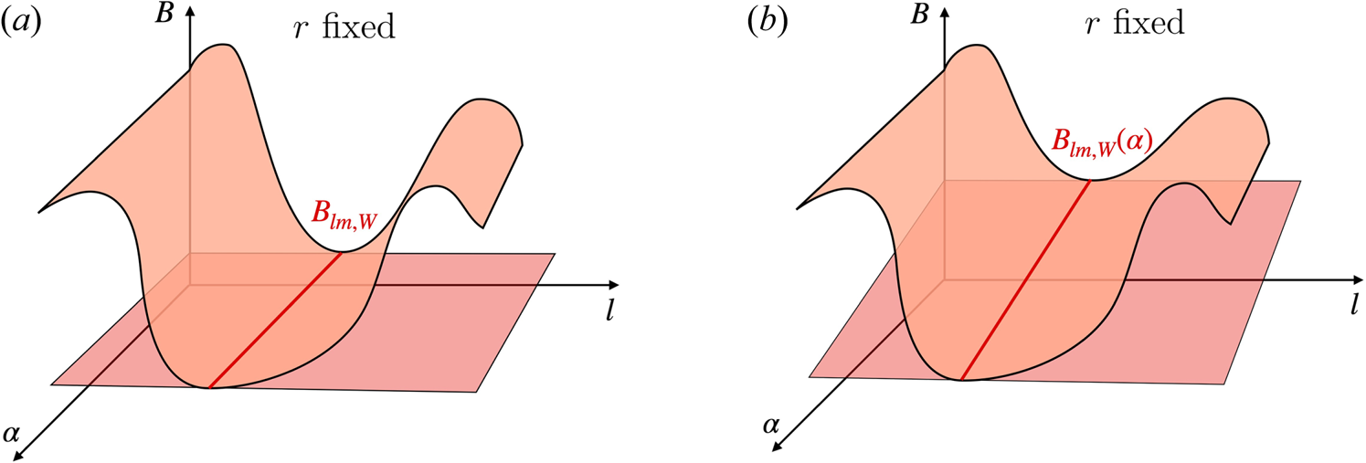
In a generic large aspect ratio stellarator with mirror ratio close to unity, the deeply trapped particles cannot move across magnetic field lines on a given flux surface, as shown on figure 4(b). However, since the electric potential $\phi _0$ varies with $r$, it is possible for $v_\parallel$ to be approximately equal to zero after a displacement $\Delta \alpha$ if the particle moves across flux surfaces by a distance $\Delta r$. Using (5.53), we find that $\Delta \alpha$ and $\Delta r$ must satisfy

(5.54)\begin{equation} 0=\mu\, \partial_{\alpha}B_{lm, W}(\alpha,r) \Delta \alpha + \frac{Z_ie \phi_0^{\prime}(r, t)}{m_i} \Delta r, \end{equation}

where we have neglected the radial derivative of $B_{lm, W}(r, \alpha )$ because it is small by a factor of $\epsilon$ compared with the radial derivative of $\phi _0$. This is consistent with the velocities $\mathrm {d}\alpha /\mathrm {d}t$ and $\mathrm {d}r / \mathrm {d}t$ obtained from the transit average drifts in (4.5) and (4.6),

(5.55)\begin{equation} \frac{\mathrm{d}\alpha}{\mathrm{d}t} \simeq \frac{c \phi_0^{\prime}}{\varPsi_t^{\prime}} \end{equation}

and

(5.56)\begin{equation} \frac{\mathrm{d}r}{\mathrm{d}t} \simeq{-}\frac{m_i c v^{2}}{2Z_i e B_0 \varPsi_t^{\prime}}\partial_{\alpha}B_{1,lm, W}, \end{equation}

where $B_{1,lm, W}(r, \alpha )$ is the local minimum of $B_1$ in well $W$ along the magnetic field line determined by $r$ and $\alpha$. Moreover, (5.54) is also consistent with the definition of the radial displacement $r_{i, 1, W}$ given in (5.26). Indeed, to lowest order in $\epsilon$, $\lambda = B_{lm, W}^{-1}$ for deeply trapped particles, and $\lambda \rightarrow B_M^{-1}$ for $J \rightarrow \infty$, giving

(5.57)\begin{equation} r_{i, 1, W} \simeq \frac{m_i v^{2}}{2Z_i e \phi_0^{\prime}} \frac{B_{1,M} (r) - B_{1, lm, W}(r, \alpha)}{B_0}. \end{equation}

This equation is a solution to (5.55) and (5.56), and it shows how the particle moves radially to increase and decrease its electric energy to keep its total energy constant.

We can draw the path followed by a deeply trapped particle with $J=0$ on an $(l,\alpha )$ plane, sketched in figure 5 for $\phi _0^{\prime } > 0$ and $\varPsi _t^{\prime } > 0$. The particle moves towards increasing $\alpha$ following the local minima $B_{lm, W}$. Simultaneously, the particle moves back and forth across flux surfaces, increasing $r$ when $\partial _{\alpha }B < 0$ or decreasing $r$ when $\partial _{\alpha }B > 0$. It is interesting to note that

(5.58)\begin{equation} \frac{\Delta r}{\Delta \alpha} \sim \epsilon a, \end{equation}

showing that the oscillating displacement across flux surfaces is much smaller that the precession around it. Equation (5.25) reproduces this motion for deeply trapped particles.

Figure 5.

Map of the magnetic field magnitude $B$ in an $(l,\alpha )$ plane. In black with arrows, we sketch the path followed by particles with $J=0$ in a stellarator with $\phi _0^{\prime } > 0$ and $\varPsi _t^{\prime } > 0$. The coordinate $r$ is not constant, and its variation around its average value has the opposite sign to the value of $B_1 = B - B_0$, as shown in (5.57).

6. The $1/\nu$ regime in large aspect ratio stellarators with mirror ratios close to unity

In this section, we briefly consider the limit $\nu _{i*} \gg \rho _{i*}$. In this limit, we can neglect the term $(c \phi _0^{\prime }/\varPsi _t^{\prime })\, \partial _\alpha g_{i, 1, W}$ in (5.25), giving to lowest order

(6.1)\begin{equation} - \frac{v^{2} \nu_{ii,\perp}(v)}{4}\, \partial_{J} \left ( \tau_W J \, \partial_{J} g_{i, 1, W} \right ) \simeq{-} \frac{c \phi_0^{\prime}}{\varPsi_t^{\prime}} \, \partial_\alpha r_{i, 1, W} \varUpsilon_i f_{Mi}. \end{equation}

This equation can be integrated using boundary condition (5.34) and relation (5.33) at the junctures of several types of wells. The final result is a trapped-particle distribution function of order $g_{i, 1, W} \sim \epsilon \rho _{i*} f_{Mi}/\nu _{i*}$. Using this result in (5.48) and (5.50) for the particle and energy fluxes, we obtain

(6.2a,b)\begin{equation} \varGamma_i \sim \frac{\rho_{i*}}{\nu_{i*}} \epsilon^{5/2} \rho_{i*} n_i v_{ti}, \quad Q_i \sim \frac{\rho_{i*}}{\nu_{i*}} \epsilon^{5/2} \rho_{i*} n_i T_i v_{ti}. \end{equation}

These are the typical $1/\nu$ regime order-of-magnitude estimates (Ho & Kulsrud Reference Ho and Kulsrud1987).

Estimates (6.2a,b) can be obtained using a random walk argument. For $\nu _{i*} \gg \rho _{i*}$, a typical trapped particle moves radially due to the radial magnetic drift $\boldsymbol {v}_{Mi} \boldsymbol {\cdot } \boldsymbol {\nabla } r \sim \epsilon \rho _{i*} v_{ti}$ until a collision detraps it. As a result, particles move a distance $\boldsymbol {v}_{Mi} \boldsymbol {\cdot } \boldsymbol {\nabla } r/\nu _\mathrm {eff}$ between collisions, where $\nu _\mathrm {eff} \sim \nu _{ii}/\epsilon$ is the effective collision frequency for trapped particles. After each detrapping collision, a trapped particle becomes passing and moves along the magnetic field line until another low angle collision reduces its parallel velocity sufficiently to trap it in a different well. The magnitude and sign of $\boldsymbol {v}_{Mi} \boldsymbol {\cdot } \boldsymbol {\nabla } r$ in the new well will in general be different from the sign and magnitude of the radial drift in the original well because the particle has moved a significant distance along the magnetic field line while being a passing particle. For this reason, the radial displacement of a typical trapped particle is similar to a random walk with a characteristic step size $\boldsymbol {v}_{Mi} \boldsymbol {\cdot } \boldsymbol {\nabla } r/\nu _\mathrm {eff} \sim (\rho _{i*}/\nu _{i*}) \epsilon a \ll \epsilon a$ and a characteristic time $1/\nu _\mathrm {eff} \sim \epsilon /\nu _{ii}$. The corresponding diffusion coefficient is $D \sim \sqrt {\epsilon } (\boldsymbol {v}_{Mi} \boldsymbol {\cdot } \boldsymbol {\nabla } r/\nu _\mathrm {eff})^{2} \nu _\mathrm {eff}$, where $\sqrt {\epsilon }$ is the estimate for the trapped-particle fraction. With $D \sim \epsilon ^{5/2} \rho _{i*}^{2} a v_{ti}/\nu _{i*}$ and using $\varGamma _i \sim D|\boldsymbol {\nabla } n_i| \sim D n_i/a$ and $Q_i \sim n_i D |\boldsymbol {\nabla } T_i| \sim D n_i T_i/a$, we recover estimates (6.2a,b).

7. The $\nu$ regime in large aspect ratio stellarators with mirror ratios close to unity

In this section, we study the limit $\nu _{i*} \ll \rho _{i*}$. We expand $g_{i, 1, W}$ in $\nu _{i*}/\rho _{i*} \ll 1$,

(7.1)\begin{equation} g_{i, 1, W} = g_{i,1,W}^{\{0\}} + g_{i,1,W}^{\{1\}} + \cdots, \end{equation}

with $g_{i,1,W}^{\{n\}} \sim (\nu _{i*}/\rho _{i*})^{n} \epsilon f_{Mi}$. We proceed to expand (5.25) in $\nu _{i*}/\rho _{i*} \ll 1$. In § 7.1, we solve the lowest-order version of (5.25) and we show that the lowest-order distribution function does not give rise to radial fluxes of particles or energy. In § 7.2, we go to next order in $\nu _{i*}/\rho _{i*} \ll 1$. Finally, in § 7.3, we calculate the particle and energy fluxes.

7.1. Lowest-order distribution function

Equation (5.25) becomes, to lowest order in $\nu _{i*}/\rho _{i*} \ll 1$,

(7.2)\begin{equation} \frac{c\phi_0^{\prime}}{\varPsi_t^{\prime}} \partial_{\alpha} g_{i,1,W}^{\{0\}} ={-} \frac{c\phi_0^{\prime}}{\varPsi_t^{\prime}} \partial_\alpha r_{i, 1, W}\, \varUpsilon_i f_{Mi}. \end{equation}

Using the fact that $\varUpsilon _i f_{Mi}$ does not vary with $\alpha$, we obtain the expression

(7.3)\begin{equation} g_{i,1,W}^{\{0\}} (r, \alpha, v, J, t) ={-} r_{i, 1, W} \varUpsilon_i f_{Mi} + K_{i, W} (r, v, J, t), \end{equation}

where the function $K_{i, W}$ does not depend on $\alpha$.

Due to the existence of junctures between different types of wells such as the one sketched in figure 1, the function $K_{i, W}$ can be independent of $J$ in large regions of velocity space. Before we explain why, we need to consider what happens with well junctures in the limit $\nu _{i*}/\rho _{i*} \ll 1$. In this limit, it is in general impossible to impose continuity of $g_{i,1,W}$ across the juncture, or condition (5.33) that relates the derivatives $\partial _J g_{i, 1, W} \simeq \partial _J g_{i,1,W}^{\{0\} }$ on different sides of a juncture to each other. This is hardly surprising since continuity of $g_{i,1,W}$ and condition (5.33) are a result of collisions, and we have neglected collisions to lowest order. In reality, continuity and condition (5.33) are not satisfied in appearance only, because boundary layers where collisions become important can form around well junctures.

The rest of this subsection is split into three parts. In the first one, we show that collisional boundary layers only form around certain junctures, and we find a condition that $K_{i, W}$ must satisfy when these boundary layers form. In the second part, we study an example that illustrates the shape of $K_{i, W}$. We finish with a general discussion.

7.1.1. Junctures of different types of wells for very small collision frequencies

Not all well junctures are problematic and need a boundary layer. Whether a juncture has a boundary layer or not depends on the direction of the velocity in $\alpha$, $c\phi _0^{\prime }/\varPsi _t^{\prime }$, and the derivatives of the juncture coordinates $J_{c, W} (r, \alpha, v)$ with respect to $\alpha$. To explain this further, we consider the juncture in figure 1. Some particles in well $I$ leave this well if the time derivative of $J_{c, I} (r, \alpha, v)$ is negative. Indeed, if a particle with $J = J_{c, I}(r(t), \alpha (t), v(t))$ at time $t$ were to stay in well $I$, it would have to do so keeping its second adiabatic invariant constant. However, such a particle would find itself with $J > J_{c, I}(r(t+\Delta t), \alpha (t + \Delta t), v(t + \Delta t))$ at $t + \Delta t$. Since there are no possible orbits with $J > J_{c, I}$ in well $I$, the particle must have moved into well $II$ or well $III$, and in doing so, the value of $J$ of the particle has changed abruptly. This is consistent with $J$ being an adiabatic invariant: it is only constant when the motion is a slowly changing periodic orbit, a description that does not apply to a transition from one well to another. These transitions between different types of wells can be understood to be a result of the conservation of phase-space volume. The second adiabatic invariant is the phase-space volume inside a trapped orbit. When $J_{c, I}$ becomes lower than the $J$ of a particle, the phase-space volume of the particle orbit cannot be contained inside well $I$ and the particle ‘spills over’ into wells $II$ and $III$ (Dobrott & Greene Reference Dobrott and Greene1971; Cary et al. Reference Cary, Escande and Tennyson1986).

Equivalently to particles moving out of well $I$ when the time derivative of $J_{c, I}$ is negative, some particles move into well $I$ if the time derivative of $J_{c, I}$ is positive. As we will see shortly, the fact that the time derivative of $J_{c, I}$ is positive implies that particles are leaving well $II$, well $III$ or both, and since these particles must move into another well, it is intuitive that conservation of phase-space volume will force these particles to move to a well where there is ‘space’. Well $I$, with a positive time derivative of $J_{c, I}$, is such a well because at time $t$ all particles in that well have $J \leq J_{c, I} (r(t), \alpha (t), v(t))$, and hence, if no particle were to move into well $I$, at time $t + \Delta t$ there would be no particles that have second adiabatic invariant between $J_{c, I} (r(t), \alpha (t), v(t))$ and $J_{c, I} (r(t + \Delta t), \alpha (t + \Delta t), v(t + \Delta t))$.

To summarize, some particles move out of well $I$ if the time derivative of $J_{c,I}$ is negative and some particles move into well $I$ if the time derivative of $J_{c, I}$ is positive. Similarly, some particles transition out of well $II$ if the time derivative of $J_{c, II}$ is negative, and some transition into it if the time derivative of $J_{c, II}$ is positive. The signs reverse for well $III$ because the orbits in this well have $J$ larger than $J_{c, III}$. Thus, particles move out of well $III$ if the time derivative of $J_{c, III}$ is positive, and transition into it if the time derivative of $J_{c, III}$ is negative.

Since both $r$ and $v$ have time derivatives that are small in $\epsilon$, the time derivative of $J_{c, W} (r, \alpha, v)$ is simply

(7.4)\begin{equation} \frac{\mathrm{d} J_{c, W}}{\mathrm{d} t} \simeq \boldsymbol{v}_E \boldsymbol{\cdot} \boldsymbol{\nabla} \alpha\, \partial_\alpha J_{c, W} \simeq \frac{c\phi_0^{\prime}}{\varPsi_t^{\prime}}\, \partial_\alpha J_{c, W}. \end{equation}

Importantly, condition (5.27) imposes that $\partial _\alpha J_{c, I} + \partial _\alpha J_{c, II} = \partial _\alpha J_{c, III}$. With this equality, it is easy to check that, if some particles are moving into well $I$, i.e. $(c\phi _0^{\prime }/\varPsi _t^{\prime })\, \partial _\alpha J_{c, I} > 0$, some particles must be leaving well $II$, $(c\phi _0^{\prime }/\varPsi _t^{\prime })\, \partial _\alpha J_{c, II} < 0$, well $III$, ${(c\phi _0^{\prime }/\varPsi _t^{\prime })\, \partial _\alpha J_{c, III} > 0}$, or both. It cannot be the case that particles are moving into all three wells, or leaving all three wells.

Armed with the results above, we can start discussing the collisional boundary layers. There are two distinct cases to consider:

1. (i) the signs of $c\phi _0^{\prime }/\varPsi _t^{\prime }$ and $\partial _\alpha J_{c, W}$ are such that some particles leave one of the wells and move into the other two wells; in this case, there is no boundary layer around the juncture; or

2. (ii) the signs of $c\phi _0^{\prime }/\varPsi _t^{\prime }$ and $\partial _\alpha J_{c, W}$ are such that some particles leave two of the wells and move into the third well; in this case, a thin boundary layer forms around the juncture.

To illustrate what happens in the case that some particles leave one of the wells and enter the other two, we consider the following example. With the sign choices $(c\phi _0^{\prime }/\varPsi _t^{\prime })\, \partial _\alpha J_{c, I} < 0$, $(c\phi _0^{\prime }/\varPsi _t^{\prime })\, \partial _\alpha J_{c, II} > 0$ and $(c\phi _0^{\prime }/\varPsi _t^{\prime })\, \partial _\alpha J_{c, III} < 0$, some particles leave well $I$ and enter well $II$ and $III$. For small collisionality, kinetic equation (7.2) imposes that the piece of the distribution function $K_{i, W}$ is continuous along particle trajectories. Since particles are leaving well $I$ and moving into well $II$ and well $III$, the distribution function in wells $II$ and $III$ must be the same as in well $I$, that is, $K_{i,II} = K_{i,I}$ and $K_{i,III} = K_{i,I}$. Thus, there is no need for a boundary layer because the distribution is continuous. Note that this process is irreversible: if we reverse time, particles leave wells $II$ and $III$ and move into well $I$, and we will see shortly that this leads, in principle, to discontinuities in the distribution function. In our equations, collisions are the only element that introduces irreversibility, so it is surprising that they do not seem to play a role in the discussion. In reality, collisions have led to this solution indirectly. If one assumes that, due to some unknown mechanism, more particles move into well $II$ than into well $III$, giving $K_{i, II} > K_{i, III}$, the distribution function is discontinuous across the juncture. Fokker–Planck collisions impose continuity in the distribution function, and as a result we need a boundary layer around such a hypothetical juncture. Appendix H shows that it is impossible to construct such a boundary layer, a result that implies that the distribution function $K_{i, W}$ must be continuous across junctures where particles leave one well to move into the other two wells.

We proceed to consider a juncture in which particles leave two wells and enter into the third well. For example, consider the situation that arises if the signs of $\phi _0^{\prime }$, $\varPsi _t^{\prime }$ and the derivatives of $J_{c,I}$, $J_{c,II}$ and $J_{c,III}$ with respect to $\alpha$ imply that particles leave wells $I$ and $II$ to enter well $III$. In this case, in general, $K_{i,I}$ and $K_{i,II}$ are different and we need to obtain a value for $K_{i,III}$. One can think of this problem as particles flowing into the juncture from wells $I$ and $II$, mixing inside the juncture, and leaving through well $III$ with a new distribution function $K_{i, III}$. A collisional boundary layer, described in Appendix H, forms around any juncture in which particles move out of two wells and into the third. The result of this boundary layer is simply a balance among the phase-space fluxes of particles across the juncture. The infinitesimal element of phase-space volume integrated over the gyrophase and $l$ can be constructed from (2.18) and (4.13), and it is $(2{\rm \pi} \varPsi _t^{\prime } v/B_0)\, \mathrm {d} r\, \mathrm {d} \alpha \, \mathrm {d} v \, \mathrm {d} J$ to lowest order in $\epsilon$. With this phase-space volume element, we can calculate the number of particles crossing $J = J_{c,W}$. One first replaces the variable $J$ with $\Delta J_W := J - J_{c, W}$. With this new set of coordinates, the infinitesimal phase-space volume becomes $(2{\rm \pi} \varPsi _t^{\prime } v/B_0)\, \mathrm {d} r\, \mathrm {d} \alpha \, \mathrm {d} v \, \mathrm {d} \Delta J_W$. Then, the rate at which phase-space volume crosses the boundary $J = J_{c, W}$, equivalent to $\Delta J_W = 0$, is

(7.5)\begin{equation} \frac{2{\rm \pi} \varPsi_t^{\prime} v}{B_0}\frac{\mathrm{d} \Delta J_W}{\mathrm{d} t}\, \mathrm{d} r\, \mathrm{d} \alpha\, \mathrm{d} v ={-} \frac{2{\rm \pi} c \phi_0^{\prime} v}{B_0} \partial_\alpha J_{c, W}\, \mathrm{d} r\, \mathrm{d} \alpha\, \mathrm{d} v, \end{equation}

where we have used (7.4) and the fact that the time derivative of $J$ is zero to obtain $\mathrm {d} \Delta J_W/\mathrm {d} t \simeq - (c \phi _0^{\prime }/\varPsi _t^{\prime }) \, \partial _\alpha J_{c, W}$. Using (7.5), we find that the number of particles crossing the boundary is $- (2{\rm \pi} c \phi _0^{\prime } v g_{i,1,W}^{\{ 0 \} }/B_0)\, \partial _\alpha J_{c, W} \, \mathrm {d} r\, \mathrm {d} \alpha \, \mathrm {d} v$. Balance between the three fluxes leaving and entering the juncture in figure 1 gives

(7.6)\begin{align} & - \frac{2{\rm \pi} c \phi_0^{\prime} v}{B_0} g_{i,1,I}^{\{ 0 \} }\, \partial_\alpha J_{c, I} \, \mathrm{d} r\, \mathrm{d} \alpha\, \mathrm{d} v - \frac{2{\rm \pi} c \phi_0^{\prime} v}{B_0} \, g_{i,1,II}^{\{ 0 \} }\, \partial_\alpha J_{c, II} \, \mathrm{d} r\, \mathrm{d} \alpha\, \mathrm{d} v \nonumber\\ & \quad ={-} \frac{2{\rm \pi} c \phi_0^{\prime} v}{B_0} \, g_{i,1,III}^{\{ 0 \} }\, \partial_\alpha J_{c, III} \, \mathrm{d} r\, \mathrm{d} \alpha\, \mathrm{d} v. \end{align}

We can simplify this expression by dividing by $- (2{\rm \pi} c \phi _0^{\prime } v/B_0)\, \mathrm {d} r\, \mathrm {d} \alpha \, \mathrm {d} v$. Furthermore, using (7.3), we find the relationship

(7.7)\begin{gather} ( K_{i, I} - r_{i, 1, I}\, \varUpsilon_i f_{Mi} ) \partial_\alpha J_{c, I} + ( K_{i, II} - r_{i, 1, II}\, \varUpsilon_i f_{Mi} )\, \partial_\alpha J_{c, II} \nonumber\\ =( K_{i, III} - r_{i, 1, III}\, \varUpsilon_i f_{Mi} )\, \partial_\alpha J_{c, III}. \end{gather}

The definition $r_{i, 1, W}$ in (5.26) implies that $r_{i, I} = r_{i, II} = r_{i, III}$ at the juncture because all the particles on the juncture have the same value of $\bar {\lambda } \simeq \lambda$. With this result and the fact that condition (5.27) gives $\partial _\alpha J_{c, I} + \partial _\alpha J_{c, II} = \partial _\alpha J_{c, III}$, all the terms that contain $r_{i, 1, W}$ cancel each other, leaving

(7.8)\begin{equation} K_{i, I}\, \partial_\alpha J_{c, I} + K_{i,II}\, \partial_\alpha J_{c,II} = K_{i, III} \, \partial_\alpha J_{c, III}. \end{equation}

Equation (7.8) can be used to calculate $K_{i,III}$ given $K_{i,I}$ and $K_{i,II}$. Note that, due to condition (5.27), $K_{i,III}$ is equal to both $K_{i,I}$ and $K_{i,II}$ if $K_{i,I} = K_{i,II}$.

The discussion in this section is related to the probabilities of transition calculated by Cary et al. (Reference Cary, Escande and Tennyson1986). If instead of the particle distribution function, one considers individual particle motion across a juncture, the problem with junctures is reversed. When a particle leaves one well to move into two other wells, the particle cannot be split into two. The exact position of the trapped particle along its quasi-periodic motion (that is, its phase) when it reaches the juncture determines the well that it moves into. Orbit-averaged motion ignores this phase, but one can assume that particles are equally distributed along this phase and, using this assumption, obtain the probability of transitioning into one well or the other. Following Cary et al. (Reference Cary, Escande and Tennyson1986), if a particle leaves well $I$, $(c\phi _0^{\prime }/\varPsi _t^{\prime })\, \partial _\alpha J_{c, I} < 0$, to move into either well $II$, $(c\phi _0^{\prime }/\varPsi _t^{\prime })\, \partial _\alpha J_{c, II} > 0$, or well $III$, $(c\phi _0^{\prime }/\varPsi _t^{\prime })\, \partial _\alpha J_{c, III} < 0$, the probability that it moves into well $II$ is $- \partial _\alpha J_{c, II}/\partial _\alpha J_{c, I}$, whereas the probability that it transitions to well $III$ is $\partial _\alpha J_{c, III}/\partial _\alpha J_{c, I}$. Thus, for single particle motion, the derivatives of $J_{c, W}$ with respect to $\alpha$ enter in the problem, but they apply to the junctures in which the particle leaves one well to move into one of the other two wells, instead of applying to the case in which particles leave two wells to transition into the third well. In this latter type of juncture, a single particle leaving one of the wells does not have any other choice but to move into the well that is accepting particles. To summarize, our formulation does not require transition probabilities because it is based on the distribution function instead of single particle motion and because, by keeping collisions, it develops the collisional boundary layers described in Appendix H.

7.1.2. Example

After explaining how the distribution function behaves around junctures of different types of wells, we proceed to argue that the function $K_{i, W}$ is independent of $J$ in large regions of velocity space. To illustrate the problem, we consider the simple situation sketched in figure 6. In this figure, we show the dependence of the effective potential $U \simeq \mu B + Z_i e \phi _0/m_i$ on $l$ for several values of $\alpha$. We consider particle motion in this effective potential for a radial electric field that forces particles to move in the direction of increasing $\alpha$, that is, $c\phi _0^{\prime }/\varPsi _t^{\prime } > 0$. Due to the changes in the $U$ profile with $\alpha$, we can divide the motion into four steps:

1. (i) Step (a) $\to$ (b). The minimum of well $II$ decreases with $\alpha$, while well $I$ does not change. Thus, $\partial _\alpha J_{c, II} > 0$ and $\partial _\alpha J_{c, III} > 0$, but $\partial _\alpha J_{c, I} = 0$. Since $c\phi _0^{\prime }/\varPsi _t^{\prime } > 0$, the discussion of the previous section implies that particles in well $III$ with low values of $J$ transition into well $II$. Particles cannot transition into well $I$ because $\partial _\alpha J_{c, I} = 0$.

2. (ii) Step (b) $\to$ (c). The minimum of well $I$ decreases, while well $II$ does not change. Hence, $\partial _\alpha J_{c, I} > 0$, $\partial _\alpha J_{c, II} = 0$ and $\partial _\alpha J_{c, III} > 0$, and particles in well $III$ with low values of $J$ transition into well $I$. Particles cannot transition into well $II$ because $\partial _\alpha J_{c, II} = 0$.

3. (iii) Step (c) $\to$ (d). The minimum of well $II$ increases until it reaches the value it had in (a), while well $I$ does not change. As a result, $\partial _\alpha J_{c, I} = 0$, $\partial _\alpha J_{c, II} < 0$ and $\partial _\alpha J_{c, III} < 0$, and particles that had transitioned into well $II$ during step (i) go back into well $III$, but their value of $J$ is greater than their initial one. Particles cannot transition into well $I$ because $\partial _\alpha J_{c, I} = 0$.

4. (iv) Step (d) $\to$ (e). The minimum of well $I$ increases until it reaches the value it had in (a), while well $II$ does not change. Then, $\partial _\alpha J_{c, I} < 0$, $\partial _\alpha J_{c, II} = 0$ and $\partial _\alpha J_{c, III} < 0$, and particles that had transitioned into well $I$ during step (ii) go back into well $III$, but their value of $J$ is lower than their initial one. Particles cannot transition into well $II$ because $\partial _\alpha J_{c, II} = 0$.

Figure 6.

Example of effective potential $U(\alpha, l)$. Each panel corresponds to a particular value of $\alpha$.

In the configuration in figure 6, there is only one juncture between wells $I$, $II$ and $III$. This juncture is characterized by the functions $J_{c, I} (r, \alpha, v)$, $J_{c, II} (r, \alpha, v)$ and $J_{c, III} (r, \alpha, v)$, sketched in figure 7(b). Each of these functions has a maximum and a minimum in $\alpha$ that we denote $J_{c, W, M} (r, v)$ and $J_{c, W, m} (r, v)$, respectively. Particles in well $I$ with values of $J$ smaller than $J_{c, I, m} (r, v)$ never transition to wells $II$ or $III$. Similarly, particles in well $II$ with $J$ smaller than $J_{c, II, m}(r, v)$ and particles in well $III$ with $J$ larger than $J_{c, III, M} (r, v)$ do not transition into the other two wells. In these regions of velocity space, the dependence of $K_{i, W}$ on $J$ will be determined in § 7.2.

Figure 7.

Evolution of the value of $J$ of a particle in the magnetic field sketched in figure 6. We start with a particle in well $III$ with initial value of the second adiabatic invariant $J = J_{\mathrm {in},0}$. Panel (a) shows the second adiabatic invariant of particles with $J = J_{III, \mathrm {in}}$ after these particles has transition into well $I$ (dark pink straight line) or well $II$ (light pink straight line), and then back to well $III$. The trajectory of the particle with initial second adiabatic invariant $J_{\mathrm {in}, 0}$ is represented by the black staircase-like line. Panel (b) shows the initial part of the same trajectory in the plane $(\alpha, J)$. The pink lines are $J_{c, I} (\alpha )$, $J_{c, II} (\alpha )$ and $J_{c, III} (\alpha )$.

The situation is very different for particles in well $III$ that have $J_{c, III, m} (r, v) < J < J_{c, III, M} (r, v)$. These particles transition into wells $I$ and $II$ and eventually transition back into well $III$. There is a value of $J$, $J_{I, II} (r, v) := J_{c, I, m} (r, v) + J_{c, II, M}(r, v)$, such that particles in well $III$ with $J_{c, III, m} < J < J_{I, II}$ transition into well $II$, and particles with $J_{I, II} < J < J_{c, III, M}$ transition into well $I$.

To understand what happens for particles with $J_{c, III, m} < J < J_{c, III, M}$, we define the function $J_{III, \mathrm {out}} (J_{III, \mathrm {in}})$. This function determines the value of the second adiabatic invariant of a particle in well $III$ after it has transitioned into well $I$ or well $II$ and has then transitioned back to well $III$. The value $J_{III, \mathrm {out}}$ of the adiabatic invariant after the particle has transition in and out of well $I$ or well $II$ depends only on the value that the adiabatic invariant had before the particle transitioned, $J_{III, \mathrm {in}}$. For the magnetic field configuration in figure 6, the function $J_{III, \mathrm {out}} (J_{III, \mathrm {in}})$ is sketched in figure 7(a) as a light pink straight line for particles that transition into well $II$ ($J_{c, III, m} < J < J_{I, II}$), and as a dark pink straight line for particles that transition into well $I$ ($J_{I, II} < J < J_{c, III, M}$). To sketch the function $J_{III, \mathrm {out}} (J_{III, \mathrm {in}})$, we have used the fact that

(7.9)\begin{equation} J_{III, \mathrm{out}} (J_{III, \mathrm{in}}) = \left \{ \begin{array}{@{}ll} J_{III, \mathrm{in}} + J_{c, I, M} - J_{c, I, m}, & \text{for }J_{c, III, m} < J < J_{I, II},\\ J_{III, \mathrm{in}} - J_{c, II, M} + J_{c, II, m}, & \text{for }J_{I, II} < J < J_{c, III, M}. \end{array} \right. \end{equation}

Using the function $J_{III, \mathrm {out}} (J_{III, \mathrm {in}})$, we can schematically describe particle motion for particles with $J_{c, III, m} < J < J_{c, III, M}$. This motion is shown in figure 7(a) as a black staircase-like line with arrows. We start with a particle with initial second adiabatic invariant $J_{\mathrm {in, 0}} < J_{I, II}$. After its transitions in and out of well $II$, this particle has acquired the second adiabatic invariant $J_{III, \mathrm {out}} (J_{\mathrm {in}, 0})$, which is necessarily in the interval $[J_{c, III, m}, J_{c, III, M}]$. As a result, the particle will transition again into well $I$ or well $II$. This fact is shown in figure 7(a) by noting that $J_{III, \mathrm {out}} (J_{\mathrm {in}, 0})$ becomes $J_{\mathrm {in}, 1}$, and this particle in turn will transition in and out of well $II$ to acquire the second adiabatic invariant $J_{III, \mathrm {out}} (J_{\mathrm {in}, 1}) = J_{III, \mathrm {out}} (J_{III, \mathrm {out}} (J_{\mathrm {in}, 0}))$. In figure 7(a), the fact that $J_{\mathrm {in}, 1} = J_{III, \mathrm {out}} (J_{\mathrm {in}, 0})$ is represented as a horizontal solid line that joins $J_{III, \mathrm {out}} (J_{\mathrm {in}, 0})$ with the diagonal line $J_{III, \mathrm {out}} = J_{III, \mathrm {in}}$, shown as a dotted line, and the fact that $J_{\mathrm {in}, 1}$ becomes $J_{III, \mathrm {out}} (J_{\mathrm {in}, 1})$ is represented as a vertical dashed line from the diagonal to $J_{III, \mathrm {out}} (J_{\mathrm {in}, 1})$. Thus, in the $J_{III, \mathrm {out}}$ vs $J_{III, \mathrm {in}}$ graph, particle trajectories are the staircase-like lines sketched in figure 7(a). The initial part of the same trajectory is sketched in figure 7(b) in the $(\alpha, J)$ plane.

Figure 7(a) shows that any particle that starts with $J_{c, III, m} < J < J_{c, III, M}$ ends up sampling all possible values of the second adiabatic invariant between $J_{c, III, m}$ and $J_{c, III, M}$ unless the function $J_{III, \mathrm {out}} (J_{III, \mathrm {in}})$ is very specific – a possible special case of this kind is represented in figure 8, where particle trajectories close on themselves in a loop in the $(J, \alpha )$ plane. We expect magnetic field magnitude profiles to satisfy the necessary constraints that lead to configurations similar to the one in figure 8 only in a countable number of flux surfaces. Thus, in general, particles in well $III$ with $J$ values between $J_{c, III, m}$ and $J_{c, III, M}$ sample all possible values of $J$ between $J_{c, III, m}$ and $J_{c, III, M}$. Since $K_{i, W}$ is constant along particle trajectories (it is independent of $\alpha$ and it is continuous at the junctures of several wells because both $g_{i, 1, W}$ and $r_{i, 1, W}$ are continuous there), we find that $K_{i, III}$ does not depend on $J$ for $J_{c, III, m} < J < J_{c, III, M}$. For the same reasons, $K_{i, I}$ in the interval $[J_{c, I, m}, J_{c, I, M}]$ and $K_{i, II}$ in the interval $[J_{c, II, m}, J_{c, II, M}]$ are both independent of $J$ and equal to the value of $K_{i, III}$ in the interval $[J_{c, III, m}, J_{c, III, M}]$. In figure 9, we sketch $K_{i, W}$ for the configuration in figure 6.

Figure 8.

Function $J_{III, \mathrm {out}}(J_{III, \mathrm {in}})$ for which particle trajectories describe a loop and do not sample a finite interval of $J$.

Figure 9.

Sketch of the function $K_{i, W}$ for the case in figure 6.

7.1.3. General considerations

We have used the example in figure 6 to illustrate the dependence of $K_{i, W}$ on $J$ because of its simplicity. In this particular configuration, particles do not have the option to choose between two wells, and particles from two different wells are not forced to move into the same well at the same time (this last case requires using (7.8)). Despite the simplicity of the example, we believe that only very specific configurations allow for a $K_{i, W}$ that is not constant in $J$ in regions with junctures of different types of wells. We note that (7.8) accepts a constant $K_{i, W}$ as a solution, and our believe is that in most cases this is the only solution. Interestingly, this $K_{i, W}$ solution does not have discontinuities in $K_{i, W}$ across junctures, and hence does not have the collisional boundary layers described in Appendix H. These layers disappear only to lowest order, as we will see that they are necessary for the next-order correction in the $\nu _{i*}/\rho _{i*} \ll 1$ expansion.

For large values of $J$, there are always junctures of different types of wells (see figure 10 and the appendix of Boozer & Gardner Reference Boozer and Gardner1990), so we expect $K_{i, W}$ to be independent of $J$ above certain value of $J$. Moreover, since $r_{i, 1, W} \rightarrow 0$ for $J \rightarrow \infty$ by definition (5.26), boundary condition (5.34) imposes that $K_{i, W} = 0$ in this region. From here on, the value of $J$ at which $K_{i, W}$ vanishes is denoted by $J_{K_{i, W} = 0}$ – see figure 9 for an example of $J_{K_{i, W} = 0}$.

Figure 10.

Sketch of trajectories with large $J$ in the $(l, \alpha )$ plane. For large $J$, $\lambda$ must be close to $1/B_M$, and hence it must have bounce points at a value of $B$ close to $B_M$. In the figure, we sketch the contour $B = 1/\lambda \approx B_M$ as a thick red line (we have assumed that there is only one maximum of $B$). The total trajectory of the particle is sketched in panel (a) as a thin red line. The best way to identify a trajectory with a given $\lambda$ is to determine the location of the bounce points (note that the left bounce point $l_{bL,W}$ is on the right of the figure and the right bounce point $l_{bR,W}$ is on the left). Particles with the kind of trajectory shown in panel (a) are exposed to four junctures with other wells, as demonstrated by panels (b–e). In panel (b), if the particle moves towards negative $\alpha$, it will transition to another type of well, similarly to panel (d). In panels (c,e), the particle transitions when it moves towards positive $\alpha$.

We finish by proving that the particle and energy fluxes due to $g_{i,1,W}^{\{0\}}$ vanish. From (5.48), we obtain that the flux of particles is

(7.10)\begin{align} \varGamma_i \simeq \frac{2{\rm \pi} c \phi_0^{\prime} }{B_0 V^{\prime}} \int^{\infty}_0 \,\mathrm{d} v \sum_W \int_{\alpha_{L, W}}^{\alpha_{R, W}}\,\mathrm{d} \alpha \int^{J_{M, W}}_{J_{m, W}} \mathrm{d} J\, v \left[ \partial_\alpha ( r_{i, 1, W} K_{i, W} ) - \partial_\alpha \left ( \frac{1}{2} r_{i, 1, W}^{2} \varUpsilon_i f_{Mi} \right ) \right]. \end{align}

The particle flux vanishes due to the integral over $\alpha$ and the fact that $r_{i, 1, W}$ and $K_{i, W}$ are continuous across junctures between several wells. A similar proof shows that the ion heat flux vanishes to lowest order in $\nu _{i*}/\rho _{i*} \ll 1$.