


1. Introduction
In two-phase systems (liquid–liquid or liquid–gas), surface tension phenomena play a vital role in controlling their shape, for example, the shape of droplets, emulsions, bubbles and the flatness of a liquid layer. However, in the presence of scalar fields, such as temperature, concentration and electric charge, the system exhibits a convective motion induced by the inhomogeneity of surface tension at the liquid–gas interface, which is known as the Marangoni effect (Levich Reference Levich1962; Davies & Rideal Reference Davies and Rideal1963; Levich & Krylov Reference Levich and Krylov1969), and the corresponding instability mechanisms are referred to as thermocapillary, solutocapillary and electrocapillary, respectively (Scriven & Sternling Reference Scriven and Sternling1960; Davis Reference Davis1987).
Surface tension- or capillary-driven flows are ubiquitous in nature, biological transport processes and our day-to-day industrial products (Manikantan & Squires Reference Manikantan and Squires2020; Temprano-Coleto & Stone Reference Temprano-Coleto and Stone2024), for instance, drying paint (Pearson Reference Pearson1958), footprint of whales (Levy et al. Reference Levy, Uminsky, Park and Calambokidis2011), formation of ripples on the skinned surface of chocolate pudding near the cup centre (Probstein Reference Probstein1994), embryo and tissue growth (Gsell et al. Reference Gsell, Tlili, Merkel and Lenne2025), single crystal growth in a microgravity environment (Schwabe et al. Reference Schwabe, Scharmann, Preisser and Oeder1978), controlling the motion of surface waves (Erinin et al. Reference Erinin, Liu, Liu, Mostert, Deike and Duncan2023), the stability of foams and emulsions (Cohen-Addad, Höhler & Pitois Reference Cohen-Addad, Höhler and Pitois2013; Grassia Reference Grassia2021; Bidoire & Vermant Reference Bidoire and Vermant2025; Chatzigiannakis et al. Reference Chatzigiannakis, Alicke, Bars, Bidoire and Vermant2025; Sharma et al. Reference Sharma, Borkar, Baumli, Shi, Wu, Myung and Fuller2025) and breakup of a thread (Hameed et al. Reference Hameed, Siegel, Young, Li, Booty and Papageorgiou2008), to mention a few.
In all the applications mentioned above, surfactants appreciably reduce surface tension, leading to the onset of the solutal Marangoni flow (Palmer & Berg Reference Palmer and Berg1972; Shklyaev & Nepomnyashchy Reference Shklyaev and Nepomnyashchy2013; Morozov, Oron & Nepomnyashchy Reference Morozov, Oron and Nepomnyashchy2014; Guzmán et al. Reference Guzmán, Martínez-Pedrero, Calero, Maestro, Ortega and Rubio2022). On the other hand, in certain situations, the Marangoni flow also appears when the surface tension increases with the scalar field, resulting in an anomalous Marangoni instability (Priede et al. Reference Priede, Cramer, Bojarevics, Gelfgat, Bar-Yoseph, Yarin and Gerbeth1999; Braverman et al. Reference Braverman, Eckert, Nepomnyashchy, Simanovskii and Thess2000). The theoretical framework for the investigation of the dynamics and stability in the case of surfactants or micelles (Stebe, Lin & Maldarelli Reference Stebe, Lin and Maldarelli1991; Jensen & Grotberg Reference Jensen and Grotberg1992; Shen et al. Reference Shen, Gleason, McKinley and Stone2002; Edmonstone, Craster & Matar Reference Edmonstone, Craster and Matar2006; Craster & Matar Reference Craster and Matar2009; Craster, Matar & Papageorgiou Reference Craster, Matar and Papageorgiou2009; Karapetsas, Craster & Matar Reference Karapetsas, Craster and Matar2011; Shklyaev & Nepomnyashchy Reference Shklyaev and Nepomnyashchy2013; Morozov et al. Reference Morozov, Oron and Nepomnyashchy2014; Manikantan & Squires Reference Manikantan and Squires2020) is well established. Likewise, a colloidal suspension made of a mixture of base liquid and nanoparticles of diameter $d_p^*\sim 10-100$
nm, known as a nanofluid, displays variation of surface tension depending on the interaction between the nanoparticle and the liquid–gas interface (Tanvir & Qiao Reference Tanvir and Qiao2012; Machrafi Reference Machrafi2022). Therefore, depending on the properties of nanoparticles and carrier liquids, the nanofluid displays a non-trivial variation of surface tension with the nanoparticle concentration. Nanofluids are actively used in many practical applications, such as paint coatings, ink-jet printing (Lohse Reference Lohse2022), microgravity experiments (Vailati et al. Reference Vailati2023) and nanofluid fuels (Abramzon & Sirignano Reference Abramzon and Sirignano1989; Basu & Miglani Reference Basu and Miglani2016; Vang & Shaw Reference Vang and Shaw2020; Shaw Reference Shaw2022). Marangoni instability is also explored in complex fluids, such as viscoelastic fluids. Sarma & Mondal (Reference Sarma and Mondal2019, Reference Sarma and Mondal2021a
,
Reference Sarma and Mondalb
) investigated the onset of Marangoni convection in a pure viscoelastic fluid and viscoelastic binary liquid with different heating/cooling conditions.
$d_p^*\sim 10-100$
nm, known as a nanofluid, displays variation of surface tension depending on the interaction between the nanoparticle and the liquid–gas interface (Tanvir & Qiao Reference Tanvir and Qiao2012; Machrafi Reference Machrafi2022). Therefore, depending on the properties of nanoparticles and carrier liquids, the nanofluid displays a non-trivial variation of surface tension with the nanoparticle concentration. Nanofluids are actively used in many practical applications, such as paint coatings, ink-jet printing (Lohse Reference Lohse2022), microgravity experiments (Vailati et al. Reference Vailati2023) and nanofluid fuels (Abramzon & Sirignano Reference Abramzon and Sirignano1989; Basu & Miglani Reference Basu and Miglani2016; Vang & Shaw Reference Vang and Shaw2020; Shaw Reference Shaw2022). Marangoni instability is also explored in complex fluids, such as viscoelastic fluids. Sarma & Mondal (Reference Sarma and Mondal2019, Reference Sarma and Mondal2021a
,
Reference Sarma and Mondalb
) investigated the onset of Marangoni convection in a pure viscoelastic fluid and viscoelastic binary liquid with different heating/cooling conditions.
Legros (Reference Legros1986), Oron & Rosenau (Reference Oron and Rosenau1994) and Braverman et al. (Reference Braverman, Eckert, Nepomnyashchy, Simanovskii and Thess2000) investigated the thermocapillary instability in the case of non-monotonic variation of surface tension with temperature. Recently, Sarma & Mondal (Reference Sarma and Mondal2018) investigated the onset of Marangoni instability in a thin liquid film heated at the substrate with a non-monotonic variation of surface tension with temperature at the gas–liquid interface. They presented the onset of thermocapillary instability in both the long- and short-wave regimes. Moreover, this anomalous dependence of surface tension on temperature has found applications in heat pipes employing self-rewetting fluids (Zhang Reference Zhang2001; Abe Reference Abe2006; Batson, Agnon & Oron Reference Batson, Agnon and Oron2017). We note that the anomalous solutocapillary instability affects a broad spectrum of applications. Recently, Diddens, Dekker & Lohse (Reference Diddens, Dekker and Lohse2025) and Dekker, Diddens & Lohse (Reference Dekker, Diddens and Lohse2025) highlighted the impact of a non-monotonic variation of surface tension with concentration on spontaneous solutal Marangoni flow. The emergence of the anomalous solutocapillary instability remains unexplored. In the framework of theoretical development for colloidal dispersions, nanoparticles, in particular, additionally promote the ingredient of inhomogeneity of surface concentration, which may cause the solutal Marangoni instability.
Our earlier investigations (Gandhi et al. Reference Gandhi, Nepomnyashchy and Oron2025a , Reference Gandhi, Nepomnyashchy and Oronb , Reference Gandhi, Nepomnyashchy and Oronc ) addressed the following aspects: (i) it was assumed there that the equilibration between the bulk concentration and the surface concentration is very fast, and thus a consideration of the dynamics of the adsorbed nanoparticles as a special two-dimensional subsystem is unnecessary. In fact, the effects of adsorption and desorption were ignored there; (ii) it was assumed there that the surface tension decreases with nanoparticle concentration, which is actually valid only for relatively low concentrations of nanoparticles; (iii) the layer was subjected to heat transfer being either heated or cooled at the substrate. Therefore, the instabilities considered in Gandhi et al. (Reference Gandhi, Nepomnyashchy and Oron2025a , Reference Gandhi, Nepomnyashchy and Oronb , Reference Gandhi, Nepomnyashchy and Oronc ) resulted from the existence of surface tension gradients of temperature and concentration at the layer interface. We stress that suspensions of nanoparticles present in both the bulk of the base fluid and at the interface with the ambient gas are considered here in the case of an isothermal system, implying that all non-equilibrium effects caused by heating/cooling are absent. The presence of nanoparticles is similar to the presence of surfactants; therefore, we refer to flows induced by nanoparticles as solutocapillary flows. Thus, the goal of the present paper is to demonstrate the emergence of a qualitatively novel instability mechanism based on the anomalous solutocapillary effect and interfacial nanoparticle kinetics in an isothermal nanofluid layer. The findings of the present paper have a direct impact on various industrial processes, for instance, the stabilisation of foams, emulsions and distillation, to name just a few.
The article is arranged in the following order. Section 2 outlines the general problem formulation, comprising the model for surface tension for a colloidal dispersion, interfacial nanoparticle dynamics and dimensional and non-dimensional governing equations and boundary conditions. § 3 provides details of the equilibrium solution and linear stability analysis to obtain the linear eigenvalue problem (EVP). Section 4 presents the analytical solution and discussion on the emergence of the anomalous solutocapillary instability. Finally, § 5 summarises the findings of the present paper.
2. Problem formulation
We consider an isothermal nanofluid layer of mean thickness $h_0^*$
deposited on a rigid and impermeable horizontal substrate and exposed to a quiescent gas environment held at constant pressure
$h_0^*$
deposited on a rigid and impermeable horizontal substrate and exposed to a quiescent gas environment held at constant pressure $p^\ast _\infty$
in the gravity field
$p^\ast _\infty$
in the gravity field $g^*$
. For simplicity, we assume constant physical properties of the nanofluid, which are density
$g^*$
. For simplicity, we assume constant physical properties of the nanofluid, which are density $\rho ^*$
, dynamic viscosity
$\rho ^*$
, dynamic viscosity $\mu ^*$
and kinematic viscosity
$\mu ^*$
and kinematic viscosity $\nu ^*= \mu ^*/\rho ^*$
. We also assume that the liquid–gas interface is non-deformable, as shown in figure 1.
$\nu ^*= \mu ^*/\rho ^*$
. We also assume that the liquid–gas interface is non-deformable, as shown in figure 1.
Nanofluid layer with particles of diameter $d_p^* \sim 20$
–
$d_p^* \sim 20$
– $50 \,\text{nm}$
deposited on the solid substrate, exposed to the gas phase at its non-deformable interface with interfacial adsorption/desorption particle kinetics. Here,
$50 \,\text{nm}$
deposited on the solid substrate, exposed to the gas phase at its non-deformable interface with interfacial adsorption/desorption particle kinetics. Here, $J_a,J_d$
and
$J_a,J_d$
and $J_{Ds}$
represent the dimensionless molar nanoparticle fluxes due to adsorption, desorption and surface diffusion, respectively, whode dimensional counterparts are given in § 2.2. The
$J_{Ds}$
represent the dimensionless molar nanoparticle fluxes due to adsorption, desorption and surface diffusion, respectively, whode dimensional counterparts are given in § 2.2. The $J_D$
is the dimensionless molar diffusive flux of nanoparticles in the bulk corresponding to the dimensional molar diffusive flux
$J_D$
is the dimensionless molar diffusive flux of nanoparticles in the bulk corresponding to the dimensional molar diffusive flux $J_D^*= - D^*_B \nabla^* C^* \phi$
represents dimensionless volumetric concentration of particles in the bulk.
$J_D^*= - D^*_B \nabla^* C^* \phi$
represents dimensionless volumetric concentration of particles in the bulk.

The frame of reference used here has the $x^*$
and
$x^*$
and $y^*$
axes located on the substrate, whereas the
$y^*$
axes located on the substrate, whereas the $z^*$
axis is normal to the substrate and directed into the fluid layer. The nanofluid layer is assumed to contain particles whose volumetric bulk concentration is
$z^*$
axis is normal to the substrate and directed into the fluid layer. The nanofluid layer is assumed to contain particles whose volumetric bulk concentration is $\phi ^*(x^*,y^*,z^*,t^*)$
, which varies in space
$\phi ^*(x^*,y^*,z^*,t^*)$
, which varies in space $(x^*,y^*,z^*)$
and time
$(x^*,y^*,z^*)$
and time $t^*$
. Our recent investigation (Gandhi et al. Reference Gandhi, Nepomnyashchy and Oron2025c
) revealed that, in the case of a moderately dense nanofluid layer, the thermophysical properties do not significantly impact the threshold values of the Marangoni instabilities. Therefore, to simplify the problem at hand and reveal the underlying instability mechanisms, we assume constant density, viscosity and Brownian diffusivity. We further neglect the effects of gravity and interfacial deformability in the current setting; however, we emphasise that for the system that features the onset of Marangoni instability in the long-wave domain, gravity and interfacial deformability may become the dominant instability mechanisms.
$t^*$
. Our recent investigation (Gandhi et al. Reference Gandhi, Nepomnyashchy and Oron2025c
) revealed that, in the case of a moderately dense nanofluid layer, the thermophysical properties do not significantly impact the threshold values of the Marangoni instabilities. Therefore, to simplify the problem at hand and reveal the underlying instability mechanisms, we assume constant density, viscosity and Brownian diffusivity. We further neglect the effects of gravity and interfacial deformability in the current setting; however, we emphasise that for the system that features the onset of Marangoni instability in the long-wave domain, gravity and interfacial deformability may become the dominant instability mechanisms.
We analyse the stability of our nanofluid system for two different carrier liquids, water and tri-ethylene glycol, respectively, where the diameter of nanoparticles $d_p^*$
varies between
$d_p^*$
varies between $20$
and
$20$
and $50$
nm. We also note that nanoparticle interaction with the surrounding gas phase mediated by the carrier liquid leads to nanoparticle adsorption and desorption at/from the liquid–gas interface (Machrafi Reference Machrafi2022). In what follows, we denote the surface nanoparticle concentration by the scalar field
$50$
nm. We also note that nanoparticle interaction with the surrounding gas phase mediated by the carrier liquid leads to nanoparticle adsorption and desorption at/from the liquid–gas interface (Machrafi Reference Machrafi2022). In what follows, we denote the surface nanoparticle concentration by the scalar field $\varGamma ^*(x^*,y^*,t^*)$
. We further assume that the lateral nanoparticle interactions (Adamczyk Reference Adamczyk2012) are negligible; therefore, the influence is limited to the effects of the vertical interfacial kinetics only.
$\varGamma ^*(x^*,y^*,t^*)$
. We further assume that the lateral nanoparticle interactions (Adamczyk Reference Adamczyk2012) are negligible; therefore, the influence is limited to the effects of the vertical interfacial kinetics only.
2.1. Surface tension model of a nanofluid layer with interfacial kinetics
Fluid dispersions, such as emulsions, foams, etc. are stabilised by the adsorption of the soluble surfactants, which can be ionic and non-ionic surfactants, lipids, proteins, etc. In these solutions, the interfacial surface tension tends to decrease as described by the Gibbs adsorption equation (Kralchevsky, Danov & Denkov Reference Kralchevsky, Danov and Denkov2008; Manikantan & Squires Reference Manikantan and Squires2020)
 \begin{align} \mathrm{d}\sigma ^* = -\sum _i\varGamma _{\textit{ei}}^*\mathrm{d}\varXi ^*_i, \end{align}
where $\varGamma _{\textit{ei}}^*$
and
$\varGamma _{\textit{ei}}^*$
and $\varXi ^*_i$
are the excess surface concentration and the chemical potential of the
$\varXi ^*_i$
are the excess surface concentration and the chemical potential of the $i^{{}}$
th component, respectively. Here, we briefly present the surface tension model following the derivations given by Machrafi (Reference Machrafi2022). The Gibbs free energy of nanoparticle dispersion,
$i^{{}}$
th component, respectively. Here, we briefly present the surface tension model following the derivations given by Machrafi (Reference Machrafi2022). The Gibbs free energy of nanoparticle dispersion, $\mathcal{F}^{\kern1pt *} = -T^*_\infty \varDelta \mathscr{S}^{\kern1.5pt *}_d$
, as presented in Appendix A, accounting for both contributions, occupied and unoccupied, is given by (Machrafi Reference Machrafi2022)
$\mathcal{F}^{\kern1pt *} = -T^*_\infty \varDelta \mathscr{S}^{\kern1.5pt *}_d$
, as presented in Appendix A, accounting for both contributions, occupied and unoccupied, is given by (Machrafi Reference Machrafi2022)
 \begin{align} \mathcal{F}^{\kern1pt *} = K_B^*T_{\infty }^*N_A^*\left [\vartheta _{\textit{np}}\ln \left (\vartheta _{\textit{np}}\right ) + \vartheta _{\textit{no}}\ln \left (\vartheta _{\textit{no}}\right ) \right ], \end{align}
where $K_B^* = 1.380649\times 10^{-23}$
J K−1 is the Boltzmann constant and
$K_B^* = 1.380649\times 10^{-23}$
J K−1 is the Boltzmann constant and $N_A^* = 6.02\times 10^{23}$
mole
$N_A^* = 6.02\times 10^{23}$
mole $^{-1}$
is Avogadro’s number. Further, the non-occupied interfacial coverage is expressed via
$^{-1}$
is Avogadro’s number. Further, the non-occupied interfacial coverage is expressed via
 \begin{align} \vartheta _{\textit{no}} = 1-\vartheta _{\textit{np}}. \end{align}
The Gibbs free energy form (2.2) is consistent with the Langmuir free energy expression presented by Kralchevsky et al. (Reference Kralchevsky, Danov and Denkov2008) and Manikantan & Squires (Reference Manikantan and Squires2020). With an expression of the free energy of a nanoparticle dispersion (2.2) at hand, we now deduce the expressions for the chemical potential and the surface tension. The chemical potential for a nanofluid, kept at the constant temperature $T^*$
and the area, is given by
$T^*$
and the area, is given by
 \begin{align} \varXi ^*_{\textit{np}} = N_A^*\frac {\partial }{\partial n_{\textit{np}}}\left (\frac {n_{\textit{np}} + n_{\textit{no}}}{N_A^*}\mathcal{F}^{\kern1pt *}\right )_{T^*,n_{\textit{no}}}. \end{align}
The chemical potential, representing the free energy cost of one additional nanoparticle to adsorb at the interface, is found as
 \begin{align} \varXi ^*_{\textit{np}} = K_B^*T^*_{\infty }N_A^*\left [\ln \left (\vartheta _{\textit{np}}\right )-\omega _{\textit{np}}\ln \left (1-\vartheta _{\textit{np}}\right )\right ]\!. \end{align}
Here,
 \begin{align} \omega _{\textit{np}} = \frac {(\rho _{\textit{bf}}^*/\mathcal{M}_{\textit{bf}}^*)\mathcal{L}_{\textit{bf}}^*}{(\rho _{\textit{np}}^*/\mathcal{M}_{\textit{np}}^*)\mathcal{L}_{\textit{np}}^*}, \end{align}
is the parameter which represents the ratio between the specific interfacial area per mole occupied by nanoparticles to that covered by the base fluid molecules, where
 \begin{align} \quad \mathcal{L}_{\textit{bf}}^\ast = \frac {1}{3} \left (\frac {3\mathcal{M}_{\textit{bf}}^\ast }{4\pi \rho _{\textit{bf}}^\ast N_A^\ast } \right )^{1/3},\quad \mathcal{L}_{\textit{np}}^* = \frac {d_p^*}{3}, \end{align}
and $\rho _{\textit{bf}}^*$
and
$\rho _{\textit{bf}}^*$
and $\mathcal{M}_{\textit{bf}}^*$
denote the base fluid density and the molar mass, respectively, and the factor
$\mathcal{M}_{\textit{bf}}^*$
denote the base fluid density and the molar mass, respectively, and the factor
 \begin{align} \frac {\rho _{\textit{np}}^*}{\mathcal{M}_{\textit{np}}^*} = \left [\frac {4\pi ^2}{9\sqrt {2}}\left (\frac {d_p^*}{2}\right )^3N_A^*\right ]^{-1} \end{align}
yields the ratio of an equivalent bulk nanoparticle concentration volume fraction to the interfacial molar mass, in units of mol m− $^3$
. The values
$^3$
. The values $\mathcal{L}^*_{\textit{bf}}$
and
$\mathcal{L}^*_{\textit{bf}}$
and $\mathcal{L}^*_{\textit{np}}$
represent the effective radius of the base fluid molecule and that of the nanoparticle, respectively, both in units of m. Furthermore, we note that for
$\mathcal{L}^*_{\textit{np}}$
represent the effective radius of the base fluid molecule and that of the nanoparticle, respectively, both in units of m. Furthermore, we note that for $\omega _{\textit{np}}=1$
, the chemical potential (2.5), effectively, converges to the standard non-interacting Langmuir model of surfactant solution. The molar mass of a nanoparticle is given by
$\omega _{\textit{np}}=1$
, the chemical potential (2.5), effectively, converges to the standard non-interacting Langmuir model of surfactant solution. The molar mass of a nanoparticle is given by
 \begin{align} \mathcal{M}_{\textit{np}}^* = \mathcal{M}_{\textit{np}}^{*\prime }f_{\textit{np}}\frac {\mathcal{V}_{\textit{np}}^{\kern1.5pt *}}{\mathcal{V}_{\textit{np}}^{\kern1.5pt *\prime }}, \end{align}
where $\mathcal{M}_{\textit{np}}^{*\prime }$
and
$\mathcal{M}_{\textit{np}}^{*\prime }$
and $\displaystyle {f_{\textit{np}} = {\pi }/{3\sqrt {2}}}$
denote the molar mass of one molecule and maximum three-dimensional nanoparticle packing density, e.g. face-centred cubic array of spheres, respectively. It follows that the volumes of a nanoparticle and a spherical molecule are defined, respectively, as:
$\displaystyle {f_{\textit{np}} = {\pi }/{3\sqrt {2}}}$
denote the molar mass of one molecule and maximum three-dimensional nanoparticle packing density, e.g. face-centred cubic array of spheres, respectively. It follows that the volumes of a nanoparticle and a spherical molecule are defined, respectively, as:
 \begin{align} \mathcal{V}_{\textit{np}}^{*} = \frac {4\pi }{3}\left (\frac {d_p^*}{ 2}\right )^3\quad \text{and}\quad \mathcal{V}_{\textit{np}}^{*\prime } = \frac {4\pi }{3}\ell _{\textit{np}}^{*3};\quad \ell _{\textit{np}}^{*} = \left (\frac {3\mathcal{M}_{\textit{np}}^{*\prime }}{4\pi \rho _{\textit{np}}^*N_A^*}\right )^{1/3}. \end{align}
Here, $\ell _{\textit{np}}^{*}$
depicts the radius of a molecule. Likewise, we deduce the surface chemical potential of bulk liquid molecules, as
$\ell _{\textit{np}}^{*}$
depicts the radius of a molecule. Likewise, we deduce the surface chemical potential of bulk liquid molecules, as
 \begin{align} \varXi ^*_{\textit{bf}} = K_B^*T^*_{\infty }N_A^*\omega _{\textit{bf}}\ln \left (1-\vartheta _{\textit{np}}\right ), \end{align}
which, intuitively, represents the thermal energy cost of the base molecule to acquire the unoccupied space at the interface. We note that, since the base fluid molecules and molecules in the unoccupied surface area are equivalent, $\omega _{\textit{bf}}=1$
.
$\omega _{\textit{bf}}=1$
.
In what follows, the Gibbs adsorption equation
 \begin{align} \int _{\sigma _r^*}^{\sigma ^*}\mathrm{d}\sigma ^* = -\int _0^{\vartheta _{\textit{np}}}\varGamma _e^*\mathrm{d}\varXi ^*_{\textit{np}}, \end{align}
is then integrated to obtain an expression for surface tension $\sigma ^*$
as a function of surface and bulk particle concentrations. We note that the lower limit
$\sigma ^*$
as a function of surface and bulk particle concentrations. We note that the lower limit $\sigma _r^*$
in (2.12) corresponds to the equilibrium reference value related to the clean surface. Here, the excess interfacial concentration
$\sigma _r^*$
in (2.12) corresponds to the equilibrium reference value related to the clean surface. Here, the excess interfacial concentration $\varGamma _e^*$
is obtained by subtracting the maximum interfacial concentration in the occupied space and the surface equivalent imaginary bulk concentration (see Appendix B), thus
$\varGamma _e^*$
is obtained by subtracting the maximum interfacial concentration in the occupied space and the surface equivalent imaginary bulk concentration (see Appendix B), thus
 \begin{align} \varGamma ^*_e = \vartheta _{\textit{np}}\varGamma _\infty ^*-\phi ^*\varGamma _b^* = \left (\vartheta _{\textit{np}} K_\varSigma -\phi ^*\right )\varGamma _b^*, \end{align}
where $\displaystyle {K_\varSigma = \varGamma _\infty ^\ast /\varGamma _b^\ast }$
accounts for the ability of nanoparticle to adsorb to the interface or stay in the bulk and
$\displaystyle {K_\varSigma = \varGamma _\infty ^\ast /\varGamma _b^\ast }$
accounts for the ability of nanoparticle to adsorb to the interface or stay in the bulk and $\varGamma _b^* =\displaystyle { {\mathcal{L}_{\textit{np}}^{*2}\rho _{\textit{np}}^*}/{\mathcal{L}_{\textit{bf}}^{*}\mathcal{M}_{\textit{np}}^*}}$
. Here,
$\varGamma _b^* =\displaystyle { {\mathcal{L}_{\textit{np}}^{*2}\rho _{\textit{np}}^*}/{\mathcal{L}_{\textit{bf}}^{*}\mathcal{M}_{\textit{np}}^*}}$
. Here, $\phi ^*$
represents the bulk nanoparticle concentration, and for further simplification, we denote the interfacial nanoparticle concentration
$\phi ^*$
represents the bulk nanoparticle concentration, and for further simplification, we denote the interfacial nanoparticle concentration $\varGamma ^* = \vartheta _{\textit{np}}\varGamma ^*_{\infty }$
in units of mol
$\varGamma ^* = \vartheta _{\textit{np}}\varGamma ^*_{\infty }$
in units of mol $/$
m
$/$
m $^2$
. Note that nanoparticles are neither molecules nor atoms, yet we treat them as a polymer made of many monomers, a collection of chemically connected atoms or molecules. Therefore, molar mass per volume (2.8) with the characteristic nanoparticle radius
$^2$
. Note that nanoparticles are neither molecules nor atoms, yet we treat them as a polymer made of many monomers, a collection of chemically connected atoms or molecules. Therefore, molar mass per volume (2.8) with the characteristic nanoparticle radius $\mathcal{L}_{\textit{np}}^\ast$
gives the dimension of surface nanoparticle concentration as mol
$\mathcal{L}_{\textit{np}}^\ast$
gives the dimension of surface nanoparticle concentration as mol $/$
m
$/$
m $^2$
. The maximum interfacial concentration is given by
$^2$
. The maximum interfacial concentration is given by $\displaystyle {\varGamma ^*_\infty = \vartheta _\infty \mathcal{L}_{\textit{np}}^*( {\rho _{\textit{np}}^*}/{\mathcal{M}_{\textit{np}}^*}})$
, for spherical nanoparticles, the maximum surface packing/coverage
$\displaystyle {\varGamma ^*_\infty = \vartheta _\infty \mathcal{L}_{\textit{np}}^*( {\rho _{\textit{np}}^*}/{\mathcal{M}_{\textit{np}}^*}})$
, for spherical nanoparticles, the maximum surface packing/coverage $\vartheta _\infty = 0.547$
.
$\vartheta _\infty = 0.547$
.
Finally, based on the Gibbs adsorption (2.12), we derive an expression for surface tension as a function of the surface and bulk concentration of a nanofluid, which in the isothermal case reduces to
 \begin{multline} \sigma ^*(\varGamma ^*,\,\phi ^*) = \sigma _r^* + T_\infty ^* N_A^* \varGamma _b^* K_B^* \Biggl \{-K_{\varSigma } \frac {\varGamma ^*}{\varGamma _\infty ^*} + \phi ^* \ln \left (\frac {\varGamma ^*}{\varGamma _\infty ^*}\right ) +\\\omega _{\textit{np}} \biggl [\left (K_{\varSigma }-\phi ^* \right ) \ln \left (1-\frac {\varGamma ^*}{\varGamma _\infty ^*}\right )+K_{\varSigma } \frac {\varGamma ^*}{\varGamma _\infty ^*}\biggr ] \Biggr \}. \end{multline}
It is interesting to note that, according to (2.14), the surface tension depends on both bulk and surface nanoparticle concentrations, due to the definition of excess interfacial concentration detailed in Appendix B. We note that nanoparticles are effectively the Gibbs monolayers, which represent the equilibrium between the adsorbed surface concentration $\varGamma ^*$
and the bulk nanoparticle concentration at the interface
$\varGamma ^*$
and the bulk nanoparticle concentration at the interface $\phi ^*(z^*=h_0^*)$
. This implies that, at equilibrium, the concentration variables in (2.14) are not independent but related via a thermodynamic quantity, the adsorption constant. At thermodynamic equilibrium, the total change in Gibbs free energy, which accounts for the free energy cost to adsorb one particle to the interface and the free energy liberated due to dissolution of one particle to the bulk, should be zero. Hence, at equilibrium, the interfacial nanoparticle concentration is adequately described by the standard Langmuir isotherm (Manikantan & Squires Reference Manikantan and Squires2020; Machrafi Reference Machrafi2022), a further discussion is presented in Appendix C. In the absence of empirical thermodynamic quantities, it is sufficient to describe the equilibrium condition via dynamic equilibrium, which accounts for the ratio of adsorption to desorption rate, instead of free energy (Dugyala et al. Reference Dugyala, Muthukuru, Mani and Basavaraj2016; Machrafi Reference Machrafi2022), which will be discussed in the subsequent § 2.2. We note that the equation of state for the variation of surface tension (2.14) is applicable for the system with no interfacial interparticle interactions, including direct interactions and interactions mediated by interfacial deformation (Guzmán et al. Reference Guzmán, Martínez-Pedrero, Calero, Maestro, Ortega and Rubio2022). We further stress that in situations where the interfacial particle spacing is larger than their dimension or low to moderate surface coverage
$\phi ^*(z^*=h_0^*)$
. This implies that, at equilibrium, the concentration variables in (2.14) are not independent but related via a thermodynamic quantity, the adsorption constant. At thermodynamic equilibrium, the total change in Gibbs free energy, which accounts for the free energy cost to adsorb one particle to the interface and the free energy liberated due to dissolution of one particle to the bulk, should be zero. Hence, at equilibrium, the interfacial nanoparticle concentration is adequately described by the standard Langmuir isotherm (Manikantan & Squires Reference Manikantan and Squires2020; Machrafi Reference Machrafi2022), a further discussion is presented in Appendix C. In the absence of empirical thermodynamic quantities, it is sufficient to describe the equilibrium condition via dynamic equilibrium, which accounts for the ratio of adsorption to desorption rate, instead of free energy (Dugyala et al. Reference Dugyala, Muthukuru, Mani and Basavaraj2016; Machrafi Reference Machrafi2022), which will be discussed in the subsequent § 2.2. We note that the equation of state for the variation of surface tension (2.14) is applicable for the system with no interfacial interparticle interactions, including direct interactions and interactions mediated by interfacial deformation (Guzmán et al. Reference Guzmán, Martínez-Pedrero, Calero, Maestro, Ortega and Rubio2022). We further stress that in situations where the interfacial particle spacing is larger than their dimension or low to moderate surface coverage $\vartheta _{\textit{np}}\leq 0.1$
, the interaction contribution can be safely omitted.
$\vartheta _{\textit{np}}\leq 0.1$
, the interaction contribution can be safely omitted.
It is emphasised that, under non-equilibrium conditions, the equilibrium relationship between the surface and bulk concentrations of particles does not hold anymore. Therefore, we shall consider independent disturbances for the bulk and surface concentrations of particles in our stability analysis (see its equilibrium (2.21) reached in the presence of kinetic processes, which will be considered in § 2.2.
2.2. Dynamics of interfacial nanoparticle concentration
The spatio-temporal evolution of the interfacial nanoparticle concentration $\varGamma ^*(x^*,y^*,t^*)$
at the non-deformable interface
$\varGamma ^*(x^*,y^*,t^*)$
at the non-deformable interface $z^* = const$
is given by the extension of the conservation equation derived for the case without interfacial kinetics
$z^* = const$
is given by the extension of the conservation equation derived for the case without interfacial kinetics $\mathcal{J}_a^{\kern1.5pt *} = \mathcal{J}_d^{\kern1.5pt *}=0$
(Scriven Reference Scriven1960; Edwards, Brenner & Wasan Reference Edwards, Brenner and Wasan1991; Wong, Rumschitzki & Maldarelli Reference Wong, Rumschitzki and Maldarelli1996; Pereira & Kalliadasis Reference Pereira and Kalliadasis2008; Manikantan & Squires Reference Manikantan and Squires2020)
$\mathcal{J}_a^{\kern1.5pt *} = \mathcal{J}_d^{\kern1.5pt *}=0$
(Scriven Reference Scriven1960; Edwards, Brenner & Wasan Reference Edwards, Brenner and Wasan1991; Wong, Rumschitzki & Maldarelli Reference Wong, Rumschitzki and Maldarelli1996; Pereira & Kalliadasis Reference Pereira and Kalliadasis2008; Manikantan & Squires Reference Manikantan and Squires2020)
 \begin{align} \frac {\partial \varGamma ^\ast }{\partial t^*} +{\nabla} _s^*\boldsymbol{\cdot }\left (\boldsymbol{u}_s^*\varGamma ^*\right ) = -{\nabla} _s^*\mathcal{J}_{Ds}^{\kern1.5pt *} + \varGamma _\infty ^*\mathcal{S}_a^*\left [\mathcal{J}_a^{\kern1.5pt *} - \mathcal{J}_d^{\kern1.5pt *}\right ]\!, \end{align}
where $\boldsymbol{u}_s^* \equiv (u^*,\,v^*,\,0 )$
and
$\boldsymbol{u}_s^* \equiv (u^*,\,v^*,\,0 )$
and $\displaystyle {{\nabla} _s^*\equiv (( {\partial }/{\partial x^*}),\,({\partial }/{\partial y^*}),0 )}$
are, respectively, the interface component of the velocity field and the surface gradient operator. We note that the interfacial nanoparticle evolution (2.15) is valid for the non-deformable liquid–gas interface; however, for the case of a deformable interface, the equation should incorporate the impact of compression or dilatation induced by the interfacial deformation, e.g.
$\displaystyle {{\nabla} _s^*\equiv (( {\partial }/{\partial x^*}),\,({\partial }/{\partial y^*}),0 )}$
are, respectively, the interface component of the velocity field and the surface gradient operator. We note that the interfacial nanoparticle evolution (2.15) is valid for the non-deformable liquid–gas interface; however, for the case of a deformable interface, the equation should incorporate the impact of compression or dilatation induced by the interfacial deformation, e.g. $\displaystyle {\varGamma ^* ({\nabla} _s^*\boldsymbol{\cdot }\boldsymbol{n}^* ) (\boldsymbol{u}^*\boldsymbol{\cdot }\boldsymbol{n}^* )}$
, where
$\displaystyle {\varGamma ^* ({\nabla} _s^*\boldsymbol{\cdot }\boldsymbol{n}^* ) (\boldsymbol{u}^*\boldsymbol{\cdot }\boldsymbol{n}^* )}$
, where $\boldsymbol{n}^*$
is the unit surface normal vector. The specific surface area covered by the interfacial nanoparticles per their unit mole is given by
$\boldsymbol{n}^*$
is the unit surface normal vector. The specific surface area covered by the interfacial nanoparticles per their unit mole is given by
 \begin{align} \mathcal{S}_a^* = \frac {\mathcal{M}_{\textit{np}}^{*}}{\rho _{\textit{np}}^*\mathcal{L}_{\textit{np}}^*}. \end{align}
At the non-deformable interface, the interfacial nanoparticle concentration is subjected to the fluxes due to surface diffusion $\mathcal{J}_{D_S}^*$
, the adsorption flux
$\mathcal{J}_{D_S}^*$
, the adsorption flux $\mathcal{J}_a^{\kern1.5pt *}$
and the desorption flux
$\mathcal{J}_a^{\kern1.5pt *}$
and the desorption flux $\mathcal{J}_d^{\kern1.5pt *}$
. We represent the surface diffusion flux via Fick’s law of diffusion with a constant surface diffusivity
$\mathcal{J}_d^{\kern1.5pt *}$
. We represent the surface diffusion flux via Fick’s law of diffusion with a constant surface diffusivity $D_s^*$
 \begin{align} \mathcal{J}_{Ds}^{\kern1.5pt *} = -D_s^*{\nabla} _s^*\varGamma ^*. \end{align}
We emphasise that the surface diffusivity $D_s^*$
is generally non-constant and depends on the interfacial nanoparticle concentration, as noted by Valkovska & Danov (Reference Valkovska and Danov2000) and Manikantan & Squires (Reference Manikantan and Squires2020). However, in the range of low nanoparticle concentrations, the variation of surface diffusion is quite weak. Thus, in what follows, we proceed with the constant surface diffusivity
$D_s^*$
is generally non-constant and depends on the interfacial nanoparticle concentration, as noted by Valkovska & Danov (Reference Valkovska and Danov2000) and Manikantan & Squires (Reference Manikantan and Squires2020). However, in the range of low nanoparticle concentrations, the variation of surface diffusion is quite weak. Thus, in what follows, we proceed with the constant surface diffusivity $D_s^*$
.
$D_s^*$
.
At the liquid–gas interface, the adsorption/desorption fluxes describe the nanoparticle exchange between the bulk and the interface. Here, we adopt the Langmuir isotherm model for a nanoparticle suspension, and the adsorption flux $\mathcal{J}_a^{\kern1.5pt *}$
is expressed by the adsorption of the bulk molar concentration
$\mathcal{J}_a^{\kern1.5pt *}$
is expressed by the adsorption of the bulk molar concentration $C^*$
to the available empty interfacial space
$C^*$
to the available empty interfacial space $\displaystyle (1-\varGamma ^*/\varGamma _\infty ^*)$
with the adsorption rate
$\displaystyle (1-\varGamma ^*/\varGamma _\infty ^*)$
with the adsorption rate $k_a^*$
, which yields
$k_a^*$
, which yields
 \begin{align} \mathcal{J}_a^{\kern1.5pt *} = k_a^* C^*\left (1-\frac {\varGamma ^*}{\varGamma ^*_\infty }\right )\!, \end{align}
where $\displaystyle {C^* =({\rho _{\textit{np}}^*}/{\mathcal{M}_{\textit{np}}^*})\phi ^*}$
is the bulk molar nanoparticle concentration. The desorption flux
$\displaystyle {C^* =({\rho _{\textit{np}}^*}/{\mathcal{M}_{\textit{np}}^*})\phi ^*}$
is the bulk molar nanoparticle concentration. The desorption flux $\mathcal{J}_d^{\kern1.5pt *}$
of the adsorbed nanoparticles per unit area with a desorption rate
$\mathcal{J}_d^{\kern1.5pt *}$
of the adsorbed nanoparticles per unit area with a desorption rate $k_d^*$
is given by
$k_d^*$
is given by
 \begin{align} \mathcal{J}_d^{\kern1.5pt *} = \frac {k_d^*}{\mathcal{S}_a^*}\left (\frac {\varGamma ^*}{\varGamma _\infty ^*}\right )\!. \end{align}
Variation of the surface tension $\sigma ^*(\phi ^*)$
in units of N m−1 with the nanoparticle concentration
$\sigma ^*(\phi ^*)$
in units of N m−1 with the nanoparticle concentration $\phi ^*$
. (a) Variation of surface tension for a Al
$\phi ^*$
. (a) Variation of surface tension for a Al $_2$
O
$_2$
O $_3$
nanoparticle (
$_3$
nanoparticle ( $d_p^*=50$
nm) dispersion in water. The inset shows a blowup of the domain of a low nanoparticle concentration. The thick line
$d_p^*=50$
nm) dispersion in water. The inset shows a blowup of the domain of a low nanoparticle concentration. The thick line $(\boldsymbol{-})$
,
$(\boldsymbol{-})$
, $\circ$
and
$\circ$
and $\triangle$
points represent the surface tension values obtained theoretically using equations (2.14) and (2.21), and from the experiments,
$\triangle$
points represent the surface tension values obtained theoretically using equations (2.14) and (2.21), and from the experiments, $1$
(Tanvir & Qiao Reference Tanvir and Qiao2012) and
$1$
(Tanvir & Qiao Reference Tanvir and Qiao2012) and $2$
(Harikrishnan et al. Reference Harikrishnan, Dhar, Agnihotri, Gedupudi and Das2017), respectively. (b) Variation of the surface tension for an Al
$2$
(Harikrishnan et al. Reference Harikrishnan, Dhar, Agnihotri, Gedupudi and Das2017), respectively. (b) Variation of the surface tension for an Al $_2$
O
$_2$
O $_3$
(
$_3$
( $d_p^*=20$
nm) nanoparticle dispersion in tri-ethylene glycol (TEG). The thick line
$d_p^*=20$
nm) nanoparticle dispersion in tri-ethylene glycol (TEG). The thick line $(\boldsymbol{-})$
and
$(\boldsymbol{-})$
and $\star$
points correspond to the values obtained theoretically using equations (2.14) and (2.21), and from the experiment (Machrafi Reference Machrafi2022). The deviation between the results obtained theoretically and experimentally is approximately
$\star$
points correspond to the values obtained theoretically using equations (2.14) and (2.21), and from the experiment (Machrafi Reference Machrafi2022). The deviation between the results obtained theoretically and experimentally is approximately $2.5\,\%$
. Note that the axis for the experimental data in panel (b) is on the right-hand side.
$2.5\,\%$
. Note that the axis for the experimental data in panel (b) is on the right-hand side.

Henceforth, the generalised interfacial spatio-temporal evolution equation for the interfacial nanoparticle concentration is obtained by substitution of (2.17), (2.18) and (2.19) into (2.15).
At equilibrium between the adsorption and desorption fluxes
 \begin{align} \begin{split} \mathcal{J}_a^{\kern1.5pt *} ={}& \mathcal{J}_d^{\kern1.5pt *},\\ k_a^* \frac {\rho _{\textit{np}}^*}{\mathcal{M}_{\textit{np}}^*}\phi ^*\left (1-\frac {\varGamma ^*}{\varGamma ^*_\infty }\right ) = {}& \frac {k_d^*}{\mathcal{S}_a^*}\left (\frac {\varGamma ^*}{\varGamma _\infty ^*}\right )\!, \end{split} \end{align}
thus, the dimensionless surface coverage $\displaystyle {\vartheta _{\textit{np}} = \varGamma ^\ast /\varGamma _\infty ^\ast }$
is given by
$\displaystyle {\vartheta _{\textit{np}} = \varGamma ^\ast /\varGamma _\infty ^\ast }$
is given by
 \begin{align} \vartheta _{\textit{np}} = \frac {\phi ^*k_a^*\mathcal{S}_a^*}{\left (\frac {\mathcal{M}_{\textit{np}}^*}{\rho _{\textit{np}}^*}\right )k_d^* + \phi ^*k_a^*\mathcal{S}_a^*}. \end{align}
Equation (2.21) can now be substituted in (2.14) to yield an expression for surface tension that shows its dependence on the bulk nanoparticle concentration $\phi ^*$
at the interface in equilibrium condition. Figure 2 displays the variation of surface tension
$\phi ^*$
at the interface in equilibrium condition. Figure 2 displays the variation of surface tension $\sigma ^* (\phi ^* )$
with the bulk nanoparticle concentration
$\sigma ^* (\phi ^* )$
with the bulk nanoparticle concentration $\phi ^*$
at the interface, for two different nanoparticle dispersions, Al
$\phi ^*$
at the interface, for two different nanoparticle dispersions, Al $_2$
O
$_2$
O $_3$
nanoparticles (
$_3$
nanoparticles ( $d_p^*=50$
nm) in water (Al
$d_p^*=50$
nm) in water (Al $_2$
O
$_2$
O $_3$
–W), figure 2(a), and Al
$_3$
–W), figure 2(a), and Al $_2$
O
$_2$
O $_3$
nanoparticles (
$_3$
nanoparticles ( $d_p^*=20$
nm) in tri-ethylene glycol (Al
$d_p^*=20$
nm) in tri-ethylene glycol (Al $_2$
O
$_2$
O $_3$
–TEG), figure 2(b). We observe that the Al
$_3$
–TEG), figure 2(b). We observe that the Al $_2$
O
$_2$
O $_3$
–W suspension exhibits a steady increase in surface tension with the nanoparticle concentration, as shown in figure 2(a). We ascribe this to the weak surface energetics of alumina nanoparticles in water. This implies that with an increase in interfacial concentration, the nanoparticle weakly attaches to the interface only for the lower limit of the nanoparticle concentration, where a mild bend in the surface tension is observed in the inset of figure 2(a).
$_3$
–W suspension exhibits a steady increase in surface tension with the nanoparticle concentration, as shown in figure 2(a). We ascribe this to the weak surface energetics of alumina nanoparticles in water. This implies that with an increase in interfacial concentration, the nanoparticle weakly attaches to the interface only for the lower limit of the nanoparticle concentration, where a mild bend in the surface tension is observed in the inset of figure 2(a).
On the other hand, figure 2(b) displays a noticeable decrease in surface tension with an increase in the nanoparticle concentration up to $\phi ^* \approx 0.003$
, which indicates that for small values of nanoparticle concentration, the alumina nanoparticle in tri-ethylene glycol strongly adsorbs at the liquid–gas interface and subsequently lowers the surface tension. For higher values of
$\phi ^* \approx 0.003$
, which indicates that for small values of nanoparticle concentration, the alumina nanoparticle in tri-ethylene glycol strongly adsorbs at the liquid–gas interface and subsequently lowers the surface tension. For higher values of $\phi ^*$
, the advancing nanoparticles feel the presence of already adsorbed nanoparticles at the liquid–gas interface, which leads to an increase in the surface tension. Furthermore, we note that the experimental results (Tanvir & Qiao Reference Tanvir and Qiao2012; Machrafi Reference Machrafi2022) show a good agreement with the theoretical model, with a deviation of
$\phi ^*$
, the advancing nanoparticles feel the presence of already adsorbed nanoparticles at the liquid–gas interface, which leads to an increase in the surface tension. Furthermore, we note that the experimental results (Tanvir & Qiao Reference Tanvir and Qiao2012; Machrafi Reference Machrafi2022) show a good agreement with the theoretical model, with a deviation of $2.5\,\%$
in figure 2(b).
$2.5\,\%$
in figure 2(b).
2.3. Governing equations and boundary conditions
The set of equations that govern the dynamics of a nanofluid layer contains the continuity equation in its incompressible version due to significantly low values of particle diffusion and moderate values of average bulk nanoparticle concentration $\varPhi ^*\leqslant 0.1$
, resulting in
$\varPhi ^*\leqslant 0.1$
, resulting in ${\nabla} ^*\boldsymbol{\cdot }\boldsymbol{u}^*\approx 0$
(Gandhi et al. Reference Gandhi, Nepomnyashchy and Oron2025a
,
Reference Gandhi, Nepomnyashchy and Oronb
,
Reference Gandhi, Nepomnyashchy and Oronc
), Navier–Stokes and advection–diffusion nanoparticle mass transfer equations, respectively, (Rohsenow, Hartnett & Cho Reference Rohsenow, Hartnett and Cho1998; Batchelor Reference Batchelor2000; Colinet, Legros & Velarde Reference Colinet, Legros and Velarde2001; Bird, Stewart & Lightfoot Reference Bird, Stewart and Lightfoot2002)
${\nabla} ^*\boldsymbol{\cdot }\boldsymbol{u}^*\approx 0$
(Gandhi et al. Reference Gandhi, Nepomnyashchy and Oron2025a
,
Reference Gandhi, Nepomnyashchy and Oronb
,
Reference Gandhi, Nepomnyashchy and Oronc
), Navier–Stokes and advection–diffusion nanoparticle mass transfer equations, respectively, (Rohsenow, Hartnett & Cho Reference Rohsenow, Hartnett and Cho1998; Batchelor Reference Batchelor2000; Colinet, Legros & Velarde Reference Colinet, Legros and Velarde2001; Bird, Stewart & Lightfoot Reference Bird, Stewart and Lightfoot2002)
 \begin{align} {\nabla} ^\ast \boldsymbol{\cdot }\boldsymbol{u}^* &= 0, \\[-12pt] \nonumber \end{align}
 \begin{align} \rho ^*\left [\boldsymbol{u}^*_{t^*} + \boldsymbol{u}^*\boldsymbol{\cdot }{\nabla} ^\ast \boldsymbol{u}^*\right ] &= -{\nabla} ^\ast p^* + {\nabla} ^\ast \boldsymbol{\cdot }\boldsymbol{\tau }^*, \\[-12pt] \nonumber \end{align}
 \begin{align} \phi ^*_{t^*} + \boldsymbol{u}^*\boldsymbol{\cdot }{\nabla} ^\ast \phi ^* &={\nabla} ^\ast \boldsymbol{\cdot }\left (D_B^*{\nabla} ^\ast \phi ^*\right )\!, \end{align}
where ${\boldsymbol u}^* = (u^*,v^*,w^* )$
is the flow velocity field vector, and
${\boldsymbol u}^* = (u^*,v^*,w^* )$
is the flow velocity field vector, and $\boldsymbol{\tau }^*$
is the viscous part of the stress tensor
$\boldsymbol{\tau }^*$
is the viscous part of the stress tensor $\displaystyle \boldsymbol{\tau }^* = \mu ^\ast [{\nabla} ^\ast {\boldsymbol u^*}+ ({\nabla} ^\ast {\boldsymbol u^*} )^\intercal ]$
, where the superscript
$\displaystyle \boldsymbol{\tau }^* = \mu ^\ast [{\nabla} ^\ast {\boldsymbol u^*}+ ({\nabla} ^\ast {\boldsymbol u^*} )^\intercal ]$
, where the superscript $^\intercal$
denotes the transpose of the corresponding tensor, the subscript
$^\intercal$
denotes the transpose of the corresponding tensor, the subscript $t^\ast$
stands for a partial derivative with respect to time
$t^\ast$
stands for a partial derivative with respect to time $t^\ast$
and
$t^\ast$
and $\displaystyle {{\nabla} ^*\equiv (({\partial }/{\partial x^*}),({\partial }/{\partial y^*}), ({\partial }/{\partial z^*} ))}$
. In (2.22c
), we consider the mass flux of the nanoparticles due to Brownian diffusion with a constant diffusivity
$\displaystyle {{\nabla} ^*\equiv (({\partial }/{\partial x^*}),({\partial }/{\partial y^*}), ({\partial }/{\partial z^*} ))}$
. In (2.22c
), we consider the mass flux of the nanoparticles due to Brownian diffusion with a constant diffusivity $D_B^*$
, expressed by the Stokes–Einstein formula
$D_B^*$
, expressed by the Stokes–Einstein formula
 \begin{align} D_B^* = \frac {K_B^*T^\ast }{3\pi \mu ^\ast d_p^\ast }. \end{align}
At the solid–liquid interface $z^*=0$
, we impose two boundary conditions. The boundary conditions at the solid substrate are
$z^*=0$
, we impose two boundary conditions. The boundary conditions at the solid substrate are
 \begin{align} \boldsymbol{u}^*=0\quad \text{and}\quad \phi ^*_z = 0, \end{align}
where the former corresponds to no slip and no penetration of the flow field at the substrate, while the latter describes the zero net mass flux at the substrate.
In what follows, we consider the non-deformable liquid–gas interface exposed to the gas phase. The kinematic boundary condition for a non-deformable boundary condition at $z^*=h^*(x^*,y^*)=const$
reads
$z^*=h^*(x^*,y^*)=const$
reads
 \begin{align} \boldsymbol{u}^*\boldsymbol{\cdot }\boldsymbol{e}_{z^*} = 0, \end{align}
where $\boldsymbol{e}_{z^*}$
is the unit vector in the
$\boldsymbol{e}_{z^*}$
is the unit vector in the $z$
direction. Furthermore, because of the non-deformability of the interface, the normal stress balance on it is automatically satisfied. However, the variation of nanoparticle concentration along the interface promotes the emergence of the tangential surface tension gradient, which is balanced by the tangential viscous stress
$z$
direction. Furthermore, because of the non-deformability of the interface, the normal stress balance on it is automatically satisfied. However, the variation of nanoparticle concentration along the interface promotes the emergence of the tangential surface tension gradient, which is balanced by the tangential viscous stress
 \begin{align} \mu ^*\left (u^*_{z^*} + w^*_{x^*}\right ) = \sigma ^*_{x^*}\quad \text{and}\quad \mu ^*\big (v^*_{z^*} + w^*_{y^*}\big ) = \sigma _{y^*}^*, \end{align}
where the surface tension is given by (2.14).
The boundary condition for the bulk nanoparticle concentration is expressed by the balance between the total normal molar mass flux and the total interfacial kinetic mass flux
 \begin{align} -D_B^*C^*_{z^*} = \mathcal{J}^*_a - \mathcal{J}^*_d. \end{align}
The spatio-temporal evolution of the interfacial nanoparticle concentration obeys the boundary condition (2.15).
Finally, to obtain the closure of the problem, one more condition must be satisfied. The average molar mass of the particles $(\displaystyle {\rho _{\textit{np}}^*}/{\mathcal{M}_{\textit{np}}^*})\varPhi ^*$
with
$(\displaystyle {\rho _{\textit{np}}^*}/{\mathcal{M}_{\textit{np}}^*})\varPhi ^*$
with $\varPhi ^\ast$
being the average volume concentration of the particles is conserved, therefore
$\varPhi ^\ast$
being the average volume concentration of the particles is conserved, therefore
 \begin{align} \left (\frac {\rho _{\textit{np}}^*}{\mathcal{M}_{\textit{np}}^*}\right )I(\mathcal{D}^*)h_0^* \varPhi ^* = \left [\int _{0}^{h_0^*}\left (\iint _{\mathcal{D}^*}\frac {\rho _{\textit{np}}^*}{\mathcal{M}_{\textit{np}}^*}\phi ^*(x^*,\,y^*,\,z^*){\textrm{d}}x^*{\textrm{d}}y^*\right ){\textrm{d}}z^* \right. \nonumber \\+ \left. \iint _{\mathscr{L}^{\kern1.5pt *}}\varGamma ^*(x^*,\,y^*)\,{\textrm{d}}x^*{\textrm{d}}y^* \right ], \end{align}
where $\mathcal{D}^*$
is a projection of the flow domain onto the
$\mathcal{D}^*$
is a projection of the flow domain onto the $x^\ast -y^\ast$
plane and
$x^\ast -y^\ast$
plane and $I({\mathcal{D}^*})$
is the area of this projection, whereas
$I({\mathcal{D}^*})$
is the area of this projection, whereas $\mathscr{L}^{\kern1.5pt *}$
represents the projection of the gas–liquid interface onto the
$\mathscr{L}^{\kern1.5pt *}$
represents the projection of the gas–liquid interface onto the $x^*-y^*$
surface. We mention that the average particle concentration
$x^*-y^*$
surface. We mention that the average particle concentration $\varPhi ^*$
is multiplied by the volume, i.e.
$\varPhi ^*$
is multiplied by the volume, i.e. $I(\mathcal{D}^*)h_0^*$
, implying the mass distribution across the volume of a nanofluid layer (Edmonstone et al. Reference Edmonstone, Craster and Matar2006). This implies that the total mass of nanoparticles in the bulk and at the interface is conserved; it also suggests an inherent inhomogeneity of nanoparticle distribution in the bulk and at the interface. A needed closure of the problem is obtained by imposing a constraint (2.28) with a prescribed and fixed positive value of
$I(\mathcal{D}^*)h_0^*$
, implying the mass distribution across the volume of a nanofluid layer (Edmonstone et al. Reference Edmonstone, Craster and Matar2006). This implies that the total mass of nanoparticles in the bulk and at the interface is conserved; it also suggests an inherent inhomogeneity of nanoparticle distribution in the bulk and at the interface. A needed closure of the problem is obtained by imposing a constraint (2.28) with a prescribed and fixed positive value of $\varPhi ^*$
. We note that the condition of the constant nanoparticle averaged bulk concentration
$\varPhi ^*$
. We note that the condition of the constant nanoparticle averaged bulk concentration $\varPhi ^*$
is appropriate for the case of the quiescent base state. However, in the presence of the base state flow, the conservation of the nanoparticle mass flux or the nanoparticle concentration current should be employed (Krishnan, Beimfohr & Leighton Reference Krishnan, Beimfohr and Leighton1996; Frank et al. Reference Frank, Anderson, Weeks and Morris2003; Ramachandran & Leighton Reference Ramachandran and Leighton2008; Morris Reference Morris2020).
$\varPhi ^*$
is appropriate for the case of the quiescent base state. However, in the presence of the base state flow, the conservation of the nanoparticle mass flux or the nanoparticle concentration current should be employed (Krishnan, Beimfohr & Leighton Reference Krishnan, Beimfohr and Leighton1996; Frank et al. Reference Frank, Anderson, Weeks and Morris2003; Ramachandran & Leighton Reference Ramachandran and Leighton2008; Morris Reference Morris2020).
2.4. Dimensionless governing equations and boundary conditions
We note that the governing equations and boundary conditions (2.3) possess the rotational symmetry $x^*\leftrightarrow y^*$
and
$x^*\leftrightarrow y^*$
and $u^*\leftrightarrow v^*$
. Henceforth, we constrain our system to the two-dimensional (2-D) case in the
$u^*\leftrightarrow v^*$
. Henceforth, we constrain our system to the two-dimensional (2-D) case in the $x^*-z^*$
plane. That is sufficient because in the present paper, only linear stability theory is considered. We non-dimensionalise the governing equations and boundary conditions with the following scales:
$x^*-z^*$
plane. That is sufficient because in the present paper, only linear stability theory is considered. We non-dimensionalise the governing equations and boundary conditions with the following scales:
 \begin{align} \begin{split} \left (x^*,z^* \right )=h_0^\ast \left (x,z\right ), \quad h^\ast =h_0^\ast h,\quad {\boldsymbol{u}^*}= \frac {\nu ^\ast }{h_0^\ast } {\boldsymbol{u}}, \quad t^*=\frac {h_0^{*2}}{\nu ^\ast } t,\quad \phi ^* = \phi _m \phi ,\\ \varPhi ^* = \phi _m\varPhi ,\quad p^*=p^\ast _\infty +\frac {\mu ^*\nu ^\ast }{h_0^{*2}} p, \quad \varGamma ^* = \varGamma _\infty ^* \varGamma . \end{split} \end{align}
From here on, the quantities without an asterisk represent the variables in a dimensionless form. In what follows, we obtain the dimensionless governing equations in the form
 \begin{align} \boldsymbol{\nabla }\boldsymbol{\cdot }\boldsymbol{u} = 0, \\[-28pt] \nonumber \end{align}
 \begin{align} \boldsymbol{u}_t + \boldsymbol{u}\boldsymbol{\cdot }\boldsymbol{\nabla }\boldsymbol{u} = -\boldsymbol{\nabla }\!p +\boldsymbol{\nabla }\boldsymbol{\cdot }\boldsymbol{\tau }, \\[-28pt] \nonumber \end{align}
 \begin{align} \mathcal{S}\left (\phi _t + \boldsymbol{u}\boldsymbol{\cdot }\boldsymbol{\nabla }\phi \right ) ={\nabla} ^2\phi , \\[-12pt] \nonumber \end{align}
where $\displaystyle \boldsymbol{\nabla }\equiv (({\partial }/{\partial x}),( {\partial }/{\partial z}) )$
and
$\displaystyle \boldsymbol{\nabla }\equiv (({\partial }/{\partial x}),( {\partial }/{\partial z}) )$
and $\displaystyle \boldsymbol{\tau } =\boldsymbol{\nabla }{\boldsymbol u}+ \boldsymbol{\nabla }{\boldsymbol u}^\intercal$
is the dimensionless viscous component of the stress tensor.
$\displaystyle \boldsymbol{\tau } =\boldsymbol{\nabla }{\boldsymbol u}+ \boldsymbol{\nabla }{\boldsymbol u}^\intercal$
is the dimensionless viscous component of the stress tensor.
The dimensionless boundary conditions at the solid substrate $z=0$
are expressed by
$z=0$
are expressed by
 \begin{align} \boldsymbol{u} = 0\quad \text{and}\quad \phi _z = 0. \end{align}
The dimensionless kinematic boundary condition and the continuity of the tangential stress at $z=1$
read
$z=1$
read
 \begin{align} w=0\quad \text{and}\quad u_z + w_x = \sigma _x, \end{align}
respectively. Following (2.14), we express the dimensionless equation of state as
 \begin{align} \sigma = \varSigma _0 + E \bigg [\omega _{\textit{np}}\phi _m \left [\left (\frac {K_{\varSigma }}{\phi _m}-\phi \right ) \ln \left (1-\varGamma \right )+ \frac {K_{\varSigma }}{\phi _m} \varGamma \right ]- \phi _m\left ( \frac {K_{\varSigma }}{\phi _m} \varGamma - \phi \ln \left (\varGamma \right )\right )\biggr ], \end{align}
where $E$
is the elasticity number defined as
$E$
is the elasticity number defined as
 \begin{align} E = \frac {N_A^*\varGamma _b^*K_B^*T_\infty ^*h_0^*}{\mu ^*\nu ^*} , \end{align}
which describes the ratio of interfacial elasticity moduli at a fixed $\varGamma _b^*$
to viscous stress (Stebe et al. Reference Stebe, Lin and Maldarelli1991; Seiwert, Dollet & Cantat Reference Seiwert, Dollet and Cantat2014; Manikantan & Squires Reference Manikantan and Squires2020).
$\varGamma _b^*$
to viscous stress (Stebe et al. Reference Stebe, Lin and Maldarelli1991; Seiwert, Dollet & Cantat Reference Seiwert, Dollet and Cantat2014; Manikantan & Squires Reference Manikantan and Squires2020).
The dimensionless balance between the bulk diffusion mass flux and the interfacial nanoparticle kinetic mass flux, and the evolution equation for the interfacial nanoparticle concentration, are given by
 \begin{align} -\phi _z = \mathcal{B}_D\big [K_{\textit{ad}}\phi (1-\varGamma ) - \varGamma \big ],\quad \varGamma _{t} + (u\varGamma )_x = \mathcal{S}^{-1}_s\varGamma _{xx} + \mathcal{B}_A\big [K_{\textit{ad}}\phi (1-\varGamma ) - \varGamma \big ]. \end{align}
The non-dimensionalisation results in the following dimensionless numbers:
 \begin{align} \mathcal{S} = \frac {\nu ^*}{D_B^*},\quad \mathcal{S}_s = \frac {\nu ^*}{D_s^*},\quad \varSigma _0 = \frac {\sigma _r^*h_0^*}{\mu ^*\nu ^*}, \end{align}
where $\mathcal{S},$ $\mathcal{S}_s$
and
$\mathcal{S}_s$
and $\varSigma _0$
denote, respectively, the bulk and surface Schmidt numbers, which describe the disparity between the viscosity of the fluid and the Brownian diffusivity, and the dimensionless surface tension number.
$\varSigma _0$
denote, respectively, the bulk and surface Schmidt numbers, which describe the disparity between the viscosity of the fluid and the Brownian diffusivity, and the dimensionless surface tension number.
The investigation in the current paper focuses on the case of a non-deformable liquid–gas interface. In the case of a gravity field, the Galileo number is defined as
 \begin{align} G=\frac { g^\ast h_0^{\ast 3}}{\nu ^{\ast 2}}. \end{align}
For a layer of thickness $h^*_0=10^{-6}$
m and water as a base fluid in a terrestrial gravity
$h^*_0=10^{-6}$
m and water as a base fluid in a terrestrial gravity $g^*=9.81$
m s−
$g^*=9.81$
m s− $^2$
, the Galileo and surface tension numbers are
$^2$
, the Galileo and surface tension numbers are $G\approx 10^{-5}$
and
$G\approx 10^{-5}$
and $\varSigma _0\approx 70$
. To evaluate the relative importance of gravity and interfacial deformability, the ratio between the two, i.e. the Bond number (Takashima Reference Takashima1981), is
$\varSigma _0\approx 70$
. To evaluate the relative importance of gravity and interfacial deformability, the ratio between the two, i.e. the Bond number (Takashima Reference Takashima1981), is
 \begin{align} Bo = \frac {G}{\varSigma _0} = \frac {\rho ^*g^*h_0^{*2}}{\sigma _r^*}\sim \big (1.36\times 10^5\,\text{m}^{-2}\big )\,h_0^{*2}. \end{align}
Therefore, for a layer thickness $h_0^*=10^{-6}$
m, the Bond number
$h_0^*=10^{-6}$
m, the Bond number $Bo\approx 10^{-7}$
and in this situation, the gravity contribution can be safely omitted. The impact of interfacial deformations on the dominant regimes, long wave
$Bo\approx 10^{-7}$
and in this situation, the gravity contribution can be safely omitted. The impact of interfacial deformations on the dominant regimes, long wave $(k\sim O(\epsilon ))$
and short wave
$(k\sim O(\epsilon ))$
and short wave $(k\sim O(1))$
, with
$(k\sim O(1))$
, with $\epsilon$
being a small parameter, is estimated via (Colinet et al. Reference Colinet, Legros and Velarde2001; Nepomnyashchy, Velarde & Colinet Reference Nepomnyashchy, Velarde and Colinet2001; Gandhi et al. Reference Gandhi, Nepomnyashchy and Oron2025b
)
$\epsilon$
being a small parameter, is estimated via (Colinet et al. Reference Colinet, Legros and Velarde2001; Nepomnyashchy, Velarde & Colinet Reference Nepomnyashchy, Velarde and Colinet2001; Gandhi et al. Reference Gandhi, Nepomnyashchy and Oron2025b
)
 \begin{align} \zeta \sim \frac {1}{G+k^2\varSigma _0} , \end{align}
implying that, for the emergence of a short-wave flow, i.e. $k\sim O(1)$
,
$k\sim O(1)$
, $G\sim O( \epsilon ^2)$
and
$G\sim O( \epsilon ^2)$
and $\varSigma _0\sim O(\epsilon ^{-2})$
, the influence of interfacial deformation is negligible
$\varSigma _0\sim O(\epsilon ^{-2})$
, the influence of interfacial deformation is negligible $\zeta \ll 1$
; however, for the onset of a long-wave flow, i.e.
$\zeta \ll 1$
; however, for the onset of a long-wave flow, i.e. $k\sim O(\epsilon )$
,
$k\sim O(\epsilon )$
, $G\sim O(\epsilon ^2)$
with
$G\sim O(\epsilon ^2)$
with $\varSigma _0\sim O(1)$
or
$\varSigma _0\sim O(1)$
or $G\sim O(1)$
with
$G\sim O(1)$
with $\varSigma _0\sim O(\epsilon ^{-2})$
, the interfacial deformation
$\varSigma _0\sim O(\epsilon ^{-2})$
, the interfacial deformation $\zeta=O(1)$
, remarkably, influences the dynamics of the system. Hence, with the emergence of long-wave instability, one should revise the problem statement and include the interfacial deformation.
$\zeta=O(1)$
, remarkably, influences the dynamics of the system. Hence, with the emergence of long-wave instability, one should revise the problem statement and include the interfacial deformation.
We also estimate the relative strength of the particle flux due to the gravitational settling (Shliomis & Smorodin Reference Shliomis and Smorodin2005; Cherepanov & Smorodin Reference Cherepanov and Smorodin2019) versus the flux due to Brownian diffusion, via
 \begin{align} \mathcal{S}_g^* = \frac {h_0^*\big (\rho _{\textit{np}}^*-\rho _{\textit{bf}}^*\big )g^*\big (\pi d_p^{*3}/6\big )}{K_B^*T_\infty ^*}, \end{align}
where $\rho _{\textit{np}}^*\approx 4000$
kg m−
$\rho _{\textit{np}}^*\approx 4000$
kg m− $^3$
and
$^3$
and $\rho _{\textit{bf}}^*\approx 1000$
kg m−
$\rho _{\textit{bf}}^*\approx 1000$
kg m− $^3$
, respectively, represent the density of alumina nanoparticles and of water. Hence, for a nanoparticle of
$^3$
, respectively, represent the density of alumina nanoparticles and of water. Hence, for a nanoparticle of $d_p^*=50$
nm in a nanofluid layer of
$d_p^*=50$
nm in a nanofluid layer of $h_0^*=10^{-6}$
m, the relative sedimentation strength is
$h_0^*=10^{-6}$
m, the relative sedimentation strength is $\mathcal{S}^*_g\approx 4.6\times 10^{-4}$
; therefore, in the current investigation, the influence of gravitational sedimentation is omitted. We emphasise that, for a thicker layer
$\mathcal{S}^*_g\approx 4.6\times 10^{-4}$
; therefore, in the current investigation, the influence of gravitational sedimentation is omitted. We emphasise that, for a thicker layer $h_0^*\sim 10^{-4}$
m or a larger particle diameter
$h_0^*\sim 10^{-4}$
m or a larger particle diameter $d_p^*\approx 100$
nm, both gravity and gravitational sedimentation effects need to be taken into account.
$d_p^*\approx 100$
nm, both gravity and gravitational sedimentation effects need to be taken into account.
At the non-deformable interface, the interfacial adsorption and desorption kinetics are controlled by the following dimensionless parameters:
 \begin{align} K_{\textit{ad}} = \frac {k_a^* \rho _{\textit{np}}^*\phi _m\mathcal{S}_a^*}{\mathcal{M}_{\textit{np}}^*k_d^*}, \quad \mathcal{B}_D = \frac {k_d^*h_0^*\mathcal{M}_{\textit{np}}^{*}}{D_B^*\phi _m\mathcal{S}_a^*\rho _{\textit{np}}^*},\quad \mathcal{B}_A = \frac {k_d^*h_0^{*2}}{\nu ^*}, \end{align}
where the dimensionless parameter $K_{\textit{ad}}$
controls the interfacial adsorption/desorption kinetics through the ratio of adsorption to desorption rate. The value of the adsorption/desorption rate ratio
$K_{\textit{ad}}$
controls the interfacial adsorption/desorption kinetics through the ratio of adsorption to desorption rate. The value of the adsorption/desorption rate ratio $K_{\textit{ad}}$
can also be related to an empirically determined value
$K_{\textit{ad}}$
can also be related to an empirically determined value $\widehat {K}_{\textit{ad}}$
appearing in the Langmuir adsorption isotherm presented in (C14). Dimensionless numbers
$\widehat {K}_{\textit{ad}}$
appearing in the Langmuir adsorption isotherm presented in (C14). Dimensionless numbers $\mathcal{B}_D$
and
$\mathcal{B}_D$
and $\mathcal{B}_A$
denote the ratio of the desorption flux to the diffusion flux and to the advection flux, respectively. Furthermore, it is challenging to measure the interfacial nanoparticle concentration in experiments under the action of adsorption/desorption kinetics.
$\mathcal{B}_A$
denote the ratio of the desorption flux to the diffusion flux and to the advection flux, respectively. Furthermore, it is challenging to measure the interfacial nanoparticle concentration in experiments under the action of adsorption/desorption kinetics.
The elasticity number defined in (2.31d
) is inherently associated with the change in surface tension with interfacial nanoparticle concentration $\partial \sigma /\partial \varGamma$
and with bulk nanoparticle concentration
$\partial \sigma /\partial \varGamma$
and with bulk nanoparticle concentration $\partial \sigma /\partial \phi$
. In fact, we infer that there exist two true dynamic solutal Marangoni numbers (more specifically, Marangoni functions), namely, the surface concentration Marangoni number
$\partial \sigma /\partial \phi$
. In fact, we infer that there exist two true dynamic solutal Marangoni numbers (more specifically, Marangoni functions), namely, the surface concentration Marangoni number
 \begin{align} M_\varGamma (\varGamma ,\phi ) \equiv \frac {\partial \sigma }{\partial \varGamma } = \frac { E \left (1 -\varGamma +\varGamma \omega _{\textit{np}}\right ) \left (\varGamma K_{\varSigma }-\phi \phi _m\right )}{(\varGamma -1) \varGamma }, \end{align}
and the bulk concentration Marangoni number
 \begin{align} M_\phi (\varGamma ) \equiv \frac {\partial \sigma }{\partial \phi } = E \phi _m \left [\ln (\varGamma )- \omega _{\textit{np}} \ln (1-\varGamma )\right ]\!. \end{align}
It is interesting to note that the surface concentration Marangoni number (2.38a ) depends on both the surface and bulk nanoparticle concentrations; while the bulk concentration Marangoni number (2.38b ) depends only on the interfacial nanoparticle concentration.
Variation of solutal Marangoni numbers $M_\phi$
and
$M_\phi$
and $M_\varGamma$
with nanoparticle concentration
$M_\varGamma$
with nanoparticle concentration $\phi$
obtained from (2.31c
) in equilibrium given by (2.21) in the case of Al
$\phi$
obtained from (2.31c
) in equilibrium given by (2.21) in the case of Al $_2$
O
$_2$
O $_3$
–TEG dispersion at
$_3$
–TEG dispersion at $E\approx 2.46\times 10^{-4},$ $K_{\textit{ad}} = 1.43,$ $K_\varSigma = 10.3\times 10^{-3}$
and
$K_\varSigma = 10.3\times 10^{-3}$
and $\omega _{\textit{np}}= 0.262\times 10^3$
. The solid and dashed curves represent the variation of surface concentration Marangoni number
$\omega _{\textit{np}}= 0.262\times 10^3$
. The solid and dashed curves represent the variation of surface concentration Marangoni number $M_\varGamma$
and bulk concentration Marangoni number
$M_\varGamma$
and bulk concentration Marangoni number $M_\phi$
, respectively.
$M_\phi$
, respectively.

Figure 3 illustrates the variations with the nanoparticle concentration of the surface tension gradients with respect to the surface and bulk concentration obtained from (2.31c
) at an equilibrium interfacial nanoparticle concentration $\displaystyle \varGamma = \phi K_{\textit{ad}}/ (1+\phi K_{\textit{ad}} )$
, following from (2.21). We note that
$\displaystyle \varGamma = \phi K_{\textit{ad}}/ (1+\phi K_{\textit{ad}} )$
, following from (2.21). We note that $M_\varGamma$
monotonically (for low
$M_\varGamma$
monotonically (for low $\phi$
it may look linear, as in figure 3) increases with an increase in the nanoparticle concentration
$\phi$
it may look linear, as in figure 3) increases with an increase in the nanoparticle concentration $\phi$
. The positivity of
$\phi$
. The positivity of $M_\varGamma$
for all nanoparticle concentration values
$M_\varGamma$
for all nanoparticle concentration values $\phi$
suggests that the system may promote an intrinsic solutocapillary instability due to the surface tension gradient with respect to interfacial nanoparticle concentration. On the other hand, we observe that
$\phi$
suggests that the system may promote an intrinsic solutocapillary instability due to the surface tension gradient with respect to interfacial nanoparticle concentration. On the other hand, we observe that $M_\phi$
is negative for low bulk nanoparticle concentrations, monotonically increasing changing its sign, and then further increases with an increase in the nanoparticle concentration. Figure 3 also shows an intersection point
$M_\phi$
is negative for low bulk nanoparticle concentrations, monotonically increasing changing its sign, and then further increases with an increase in the nanoparticle concentration. Figure 3 also shows an intersection point $\tilde {M}$
corresponding to
$\tilde {M}$
corresponding to $\tilde {\phi }$
, such that,
$\tilde {\phi }$
, such that, $M_{\varGamma } \gt M_{\phi }$
for
$M_{\varGamma } \gt M_{\phi }$
for $\phi \lt \tilde {\phi }$
and
$\phi \lt \tilde {\phi }$
and $M_{\varGamma } \lt M_{\phi }$
for
$M_{\varGamma } \lt M_{\phi }$
for $\phi \gt \tilde {\phi }$
. Note that the dynamic solutal Marangoni number, specifically
$\phi \gt \tilde {\phi }$
. Note that the dynamic solutal Marangoni number, specifically $M_\varGamma$
and
$M_\varGamma$
and $M_\phi$
, converges to the known Langmuir value (Manikantan & Squires Reference Manikantan and Squires2020)
$M_\phi$
, converges to the known Langmuir value (Manikantan & Squires Reference Manikantan and Squires2020)
 \begin{align} M_\varGamma \equiv \frac {\partial \sigma }{\partial \varGamma } \sim -\frac {1}{1-\varGamma }\quad \text{and}\quad M_\phi = 0, \end{align}
in the limit of $\omega _{\textit{np}}=1$
and
$\omega _{\textit{np}}=1$
and $\varGamma _b^*=0$
equivalent to
$\varGamma _b^*=0$
equivalent to $\varGamma _e^*=\varGamma _\infty ^*\vartheta _{\textit{np}}$
before substitution into the Gibbs adsorption (2.12).
$\varGamma _e^*=\varGamma _\infty ^*\vartheta _{\textit{np}}$
before substitution into the Gibbs adsorption (2.12).
Furthermore, it is crucial to understand that the full variation of surface tension due to the solutal effects is given by
 \begin{align} \varDelta \sigma = M_\varGamma \varDelta \varGamma + M_\phi \varDelta \phi = M_\varGamma \left ( \varDelta \varGamma + \frac {M_\phi }{M_\varGamma } \varDelta \phi \right ). \end{align}
We stress that, under non-equilibrium conditions, $\varDelta \varGamma$
and
$\varDelta \varGamma$
and $\varDelta \phi$
may be independent and of either sign; therefore, it is impossible to claim whether
$\varDelta \phi$
may be independent and of either sign; therefore, it is impossible to claim whether $\varDelta \sigma$
given by (2.40) leads to the emergence of the solutocapillary instability before obtaining the solution of the EVP derived in § 3.
$\varDelta \sigma$
given by (2.40) leads to the emergence of the solutocapillary instability before obtaining the solution of the EVP derived in § 3.
The adsorption and desorption rates for the alumina nanoparticle in water (Al $_2$
O
$_2$
O $_3$
–W) and tri-ethylene glycol (Al
$_3$
–W) and tri-ethylene glycol (Al $_2$
O
$_2$
O $_3$
–TEG) are obtained by calculation of the interaction potential between a nanoparticle and the liquid–gas interface (Ruckenstein & Prieve Reference Ruckenstein and Prieve1976; Grow & Shaeiwitz Reference Grow and Shaeiwitz1982; Machrafi Reference Machrafi2022). The adsorption and desorption rates for a Al
$_3$
–TEG) are obtained by calculation of the interaction potential between a nanoparticle and the liquid–gas interface (Ruckenstein & Prieve Reference Ruckenstein and Prieve1976; Grow & Shaeiwitz Reference Grow and Shaeiwitz1982; Machrafi Reference Machrafi2022). The adsorption and desorption rates for a Al $_2$
O
$_2$
O $_3$
–W suspension (
$_3$
–W suspension ( $d_p^*=50$
nm) are
$d_p^*=50$
nm) are $k_a^* = 2.27\times 10^{-4}$
m s−1 and
$k_a^* = 2.27\times 10^{-4}$
m s−1 and $k_d^* = 2.3\times 10^3$
s
$k_d^* = 2.3\times 10^3$
s $^{-1}$
, respectively. For a Al
$^{-1}$
, respectively. For a Al $_2$
O
$_2$
O $_3$
–TEG suspension (
$_3$
–TEG suspension ( $d_p^*=20$
nm), the adsorption and desorption rates are
$d_p^*=20$
nm), the adsorption and desorption rates are $k_a^* = 4.23\times 10^{-5}$
m s−1 and
$k_a^* = 4.23\times 10^{-5}$
m s−1 and $k_d^* = 2.88\times 10^3$
s
$k_d^* = 2.88\times 10^3$
s $^{-1}$
, respectively. It should be mentioned that the disparity between interfacial kinetics rates for these two different nanoparticle suspensions varies with the nanoparticle diameter
$^{-1}$
, respectively. It should be mentioned that the disparity between interfacial kinetics rates for these two different nanoparticle suspensions varies with the nanoparticle diameter $d_p^*$
and the physical properties of the base liquid, and therefore reflects a non-trivial variation of surface tension, as shown in figure 2. The parameter ranges for other parameters used in this work are listed in table 1. Finally, following (2.28), the dimensionless version of the conservation of nanoparticles in the layer is expressed by
$d_p^*$
and the physical properties of the base liquid, and therefore reflects a non-trivial variation of surface tension, as shown in figure 2. The parameter ranges for other parameters used in this work are listed in table 1. Finally, following (2.28), the dimensionless version of the conservation of nanoparticles in the layer is expressed by
 \begin{align} I(\mathcal{D})\varPhi = \int _{0}^{1}\left (\iint _{\mathcal{D}}\phi (x,\,y,\,z){\textrm{d}}x\,{\textrm{d}}y\right ){\textrm{d}}z + \mathcal{A} \iint _{\mathscr{L}}\varGamma (x,\,y)\,{\textrm{d}}x\,{\textrm{d}}y, \end{align}
where $\displaystyle {\mathcal{A} = {\mathcal{M}_{\textit{np}}^*\varGamma _\infty ^*}/{\rho _{\textit{np}}^*h_0^*\phi _m}}$
represents the particle adsorption factor at the liquid–gas interface.
$\displaystyle {\mathcal{A} = {\mathcal{M}_{\textit{np}}^*\varGamma _\infty ^*}/{\rho _{\textit{np}}^*h_0^*\phi _m}}$
represents the particle adsorption factor at the liquid–gas interface.
Parameter nomenclature and their typical values used in this investigation.

3. Base state solution and linear stability analysis
We search for a quiescent $ (\boldsymbol{u} = \boldsymbol{u}_0 = 0 )$
steady state for the given system in terms of nanoparticle concentration
$ (\boldsymbol{u} = \boldsymbol{u}_0 = 0 )$
steady state for the given system in terms of nanoparticle concentration $\phi _0(z)$
, interfacial nanoparticle concentration
$\phi _0(z)$
, interfacial nanoparticle concentration $\varGamma _0$
and pressure
$\varGamma _0$
and pressure $p_0(z)$
. It follows from (2.30b
) and (2.30)c, and boundary conditions (2.31), that the solution is found by solving the following equations with the boundary conditions at the substrate
$p_0(z)$
. It follows from (2.30b
) and (2.30)c, and boundary conditions (2.31), that the solution is found by solving the following equations with the boundary conditions at the substrate $z=0$
and at the non-deformable interface
$z=0$
and at the non-deformable interface $z=1$
:
$z=1$
:
 \begin{align} \phi _{0,zz} = 0\quad \text{and}\quad p_{0,z} = 0, \\[-28pt] \nonumber \end{align}
 \begin{align} \phi _{0,z} = 0\quad \text{at}\quad z=0, \\[-28pt] \nonumber \end{align}
 \begin{align} \phi _{0,z} = 0,\quad p_0=0,\quad \mathcal{B}_D\left [\left (K_{\textit{ad}}\phi _0\left (1-\varGamma _0\right )\right )-\varGamma _0\right ]\quad \text{at}\quad z=1, \\[-12pt] \nonumber \end{align}
where the subscript $z$
is used to denote the differentiation with respect to
$z$
is used to denote the differentiation with respect to $z$
.
$z$
.
We deduce that the steady state bulk nanoparticle concentration $\phi _0$
is constant; however, the base state component of the interfacial nanoparticle concentration
$\phi _0$
is constant; however, the base state component of the interfacial nanoparticle concentration $\varGamma _0$
displays a jump in nanoparticle concentration due to the presence of adsorption/desorption kinetics. Additionally, in the absence of gravity and concentration stratification, the steady state pressure is zero
$\varGamma _0$
displays a jump in nanoparticle concentration due to the presence of adsorption/desorption kinetics. Additionally, in the absence of gravity and concentration stratification, the steady state pressure is zero
 \begin{align} \phi _0 = \gamma (\varPhi ),\quad \varGamma _0 = \frac {\gamma (\varPhi )K_{\textit{ad}}}{1+\gamma (\varPhi )K_{\textit{ad}}}\quad \text{and}\quad p_0 = 0. \end{align}
We note that the base state component of the bulk nanoparticle concentration is constant throughout the system. Finally, the conservation of the particle number in the bulk and at the interface is imposed by specifying the constant value of the average concentration of the nanoparticles $\varPhi$
 \begin{align} \varPhi = \phi _0 + \mathcal{A}\varGamma _0. \end{align}
For the parameter values given in table 1, $\phi _0$
is always larger than
$\phi _0$
is always larger than $\mathcal{A}\varGamma _0$
; therefore, as follows from (3.3), the bulk concentration
$\mathcal{A}\varGamma _0$
; therefore, as follows from (3.3), the bulk concentration $\phi _0$
represents the dominant component of the total number of nanoparticles in the layer.
$\phi _0$
represents the dominant component of the total number of nanoparticles in the layer.
In what follows, the value of $\gamma (\varPhi )$
is determined by substituting (3.2) into (3.3), as
$\gamma (\varPhi )$
is determined by substituting (3.2) into (3.3), as
 \begin{align} \gamma (\varPhi ) = \frac {(\varPhi - \mathcal{A}) K_{\textit{ad}}- 1 + \sqrt {4 \varPhi K_{\textit{ad}}+\left [1+(\mathcal{A}- \varPhi ) K_{\textit{ad}}\right ]^2}}{2 K_{\textit{ad}}}, \end{align}
where the constant $\gamma (\varPhi )$
depends on
$\gamma (\varPhi )$
depends on $\phi _m,$ $K_{\textit{ad}}$
and
$K_{\textit{ad}}$
and $\rho _{\textit{np}}^*/\mathcal{M}_{\textit{np}}^*$
, and is positive.
$\rho _{\textit{np}}^*/\mathcal{M}_{\textit{np}}^*$
, and is positive.
The dimensionless governing equations (2.30) and boundary conditions (2.31) are linearised around the base state (3.2) in the form
 \begin{align} \boldsymbol{u} = \boldsymbol{u}_0 + \bar {\boldsymbol{u}},\quad p = p_0 + \bar {p},\quad \phi = \phi _0 + \bar {\phi }, \quad \varGamma = \varGamma _0 + \bar {\varGamma }, \end{align}
where the terms with an overbar represent the disturbances.
The linearised set of governing equations reads in vector form
 \begin{align} \boldsymbol{\nabla }\boldsymbol{\cdot }\bar {\boldsymbol{u}} = 0,\quad \frac {\partial \bar {\boldsymbol u}}{\partial t} -{\nabla} ^2 \bar {\boldsymbol u} + \boldsymbol{\nabla }\bar p =0, \\[-28pt] \nonumber \end{align}
 \begin{align} \mathcal{S}\left [\frac {\partial \bar {\phi }}{\partial t} + \phi _0 \boldsymbol{\nabla }\boldsymbol{\cdot }\bar {\boldsymbol u} +\frac {{\textrm{d}}\phi _0}{{\textrm{d}} z}\bar {w}\right ] - {\nabla} ^2 \bar \phi =0, \\[0pt] \nonumber \end{align}
where (3.6a ) and (3.6b ) represent the linearised version of the continuity and 2-D momentum conservation and the nanoparticle advection–diffusion equations, respectively.
The linearised boundary conditions at $z=0$
are
$z=0$
are
 \begin{align} \bar {\boldsymbol{u}}=0\quad \text{and}\quad \frac {\partial \bar {\phi }}{\partial z}=0. \end{align}
At the interface $z=1$
, the linearised boundary conditions are
$z=1$
, the linearised boundary conditions are
 \begin{align} \bar {w}=0,\quad \frac {\partial \bar {u}}{\partial z} + \frac {\partial \bar {w}}{\partial x} + E \left (\alpha \frac {\partial \bar {\varGamma }}{\partial x} + \beta \frac {\partial \bar {\phi }}{\partial x} \right ) = 0, \\[-28pt] \nonumber \end{align}
 \begin{align} \frac {\partial \bar {\phi }}{\partial z}= \mathcal{B}_D\left [\chi _1\bar {\varGamma } + \chi _2 \bar {\phi }\right ],\quad \frac {\partial \bar {\varGamma }}{\partial t} + \varGamma _0\frac {\partial \bar {u}}{\partial x} - \mathcal{S}^{-1}_s\frac {\partial ^2\bar {\varGamma }}{\partial x^2} + \mathcal{B}_A\left [\chi _1\bar {\varGamma } + \chi _2 \bar {\phi }\right ] = 0, \\[0pt] \nonumber \end{align}
where, for simplicity, we introduce
 \begin{align} \left . \begin{array}{c@{}} \alpha = \frac {\left (\varGamma _0 \left (\omega _{\textit{np}}-1\right )+1\right ) \left (\varGamma _0 K_{\varSigma } - \phi _m \phi _0(1)\right )}{\left (1- \varGamma _0\right ) \varGamma _0}, \quad \beta = \phi _m \left (\ln \left (1-\varGamma _0\right ) \omega _{\textit{np}} -\ln \left (\varGamma _0\right )\right ),\\[12pt]{ \chi _1 = \phi _0 K_{\textit{ad}}+1, \quad \chi _2 = K_{\textit{ad}}\left (\varGamma _0-1\right )}. \end{array}\right \} \end{align}
We note that, in the linearised tangential stress balance (3.6d
), the perturbations of the interfacial concentration $\bar {\varGamma }$
are represented by the linearisation of the surface tension using the Taylor expansion around
$\bar {\varGamma }$
are represented by the linearisation of the surface tension using the Taylor expansion around $\varGamma _0$
. Additionally, the linearised form of the tangential stress balance (3.6d
) contains the perturbations of the two dynamic Marangoni numbers from their equilibrium state, i.e.
$\varGamma _0$
. Additionally, the linearised form of the tangential stress balance (3.6d
) contains the perturbations of the two dynamic Marangoni numbers from their equilibrium state, i.e. $M_\varGamma (\varGamma _0,\phi _0) = E\alpha$
and
$M_\varGamma (\varGamma _0,\phi _0) = E\alpha$
and $M_\phi (\varGamma _0) = E\beta$
.
$M_\phi (\varGamma _0) = E\beta$
.
We now introduce the normal perturbation modes to the system variables
 \begin{align} \left (\bar u,\,\bar {w},\,\bar {\phi },\,\bar {\varGamma }\right )\left (x,z,t\right ) = \left (u(z), \,w(z),\,\varphi (z),\,\varGamma \right )\exp (ikx+\lambda t), \end{align}
where $u,\, w,$ $\varphi $
and
$\varphi $
and $\varGamma$
are the amplitudes of the perturbations of the horizontal and vertical components of the fluid velocity field, the bulk nanoparticle concentration and the interfacial nanoparticle concentration, respectively. We determine the stability of the base state with respect to the disturbance wavenumber
$\varGamma$
are the amplitudes of the perturbations of the horizontal and vertical components of the fluid velocity field, the bulk nanoparticle concentration and the interfacial nanoparticle concentration, respectively. We determine the stability of the base state with respect to the disturbance wavenumber $k\in \mathbb{R}$
via the growth rate
$k\in \mathbb{R}$
via the growth rate $\lambda \in \mathbb{C}$
of the disturbances. In this representation, the negative and positive values of the real part of the growth rate
$\lambda \in \mathbb{C}$
of the disturbances. In this representation, the negative and positive values of the real part of the growth rate $\lambda$
correspond to the stability and instability regimes of the system, respectively.
$\lambda$
correspond to the stability and instability regimes of the system, respectively.
The Orr–Sommerfeld EVP is obtained in the form
 \begin{align} \mathcal{L}\mathsf{A} = 0, \end{align}
where the linear operator $\mathcal{L}$
and the eigenvector
$\mathcal{L}$
and the eigenvector $\mathsf{A}$
are
$\mathsf{A}$
are
 \begin{align} \mathcal{L} = \left ( \begin{array}{cc} -\left (2 k^2+\lambda \right ) \mathcal{D}^2 + k^2 \left (k^2+\lambda \right ) + \mathcal{D}^4 &\,\,\,\,\,\,\, 0 \\[10pt] 0 &\,\,\,\,\,\,\, \left (k^2+\lambda \mathcal{S}\right ) -\mathcal{D}^2 \\ \end{array} \right ), \quad \mathsf{A} = \left ( \begin{array}{c} w \\ \displaystyle \varphi \\ \end{array} \right ), \end{align}
and $\mathcal{D}^n\equiv {({d^n}/{{\textrm{d}}z^n})}$
. The EVP is subjected to the following boundary conditions:
$\mathcal{D}^n\equiv {({d^n}/{{\textrm{d}}z^n})}$
. The EVP is subjected to the following boundary conditions:
 \begin{align} w = 0,\quad \mathcal{D}w=0,\quad \mathcal{D}\varphi =0 \quad \text{at}\quad z=0. \end{align}
The boundary conditions at $z=1$
are
$z=1$
are
 \begin{align} w=0,\quad k^2 \left [E (\alpha \varGamma +\beta \varphi ) + w \right ]+ \mathcal{D}^2w = 0, \\[-28pt] \nonumber \end{align}
 \begin{align} \mathcal{B}_D \left (\varGamma \chi _1 + \chi _2 \varphi \right ) - \mathcal{D}\varphi = 0,\quad \varGamma \left (\frac {k^2}{\mathcal{S}_s}+\lambda \right )-\varGamma _0 \mathcal{D}w + \mathcal{B}_A \left (\varGamma \chi _1 + \chi _2 \varphi \right ) = 0. \\[0pt] \nonumber \end{align}
4. Results and discussions
The EVP (3.8) is solved in terms of the eigenvalue, the elasticity number $E$
. An analytical solution of this EVP is found for the case of the monotonic
$E$
. An analytical solution of this EVP is found for the case of the monotonic $(\lambda =0)$
solutocapillary instability. In the general case, the EVP (3.8) is solved numerically employing the approach based on the shooting method and the numerical construction of the complex-valued Evans function (Evans & Feroe Reference Evans and Feroe1977) and the compound matrix method (Ng & Reid Reference Ng and Reid1979). The roots of the Evans function represent the eigenvalues of the EVP (Pearce et al. Reference Pearce, Heil, Jensen, Jones and Prokop2018). More details can be found in (Gandhi et al. Reference Gandhi, Nepomnyashchy and Oron2025a
,
Reference Gandhi, Nepomnyashchy and Oronb
,
Reference Gandhi, Nepomnyashchy and Oronc
).
$(\lambda =0)$
solutocapillary instability. In the general case, the EVP (3.8) is solved numerically employing the approach based on the shooting method and the numerical construction of the complex-valued Evans function (Evans & Feroe Reference Evans and Feroe1977) and the compound matrix method (Ng & Reid Reference Ng and Reid1979). The roots of the Evans function represent the eigenvalues of the EVP (Pearce et al. Reference Pearce, Heil, Jensen, Jones and Prokop2018). More details can be found in (Gandhi et al. Reference Gandhi, Nepomnyashchy and Oron2025a
,
Reference Gandhi, Nepomnyashchy and Oronb
,
Reference Gandhi, Nepomnyashchy and Oronc
).
The general solution of the EVP (3.8) in terms of the dependent variables, $w$
and
$w$
and $\phi$
, in the case of the monotonic solutocapillary instability
$\phi$
, in the case of the monotonic solutocapillary instability $(\lambda =0)$
is found as
$(\lambda =0)$
is found as
 \begin{align} w &= e^{-k z} \left [c_3 e^{2 k z}+z \left (c_4 e^{2 k z}+c_2\right )+c_1\right ]\!, \\[-28pt] \nonumber \end{align}
 \begin{align} \varphi &= c_5 e^{k z}+c_6 e^{-k z}, \\[0pt] \nonumber \end{align}
where $c_i,\,i=1,2,\ldots ,6$
represent the integration constants whose values are to be found from the boundary conditions. The general solution (4.1) is substituted into the boundary conditions of the EVP (3.8) and a set of linear algebraic equations with constant coefficients
$c_i,\,i=1,2,\ldots ,6$
represent the integration constants whose values are to be found from the boundary conditions. The general solution (4.1) is substituted into the boundary conditions of the EVP (3.8) and a set of linear algebraic equations with constant coefficients $c_i$
is obtained, as shown in Appendix D. The solvability condition of a zero determinant of the coefficient matrix
$c_i$
is obtained, as shown in Appendix D. The solvability condition of a zero determinant of the coefficient matrix $\mathbb{M}$
of order
$\mathbb{M}$
of order $6 \times 6$
of this linear set of equations yields the marginal value of the elasticity number
$6 \times 6$
of this linear set of equations yields the marginal value of the elasticity number $E$
in the form
$E$
in the form
 \begin{align} E = \frac {2 \left [\sinh (2 k)-2 k \right ] \left [\gamma (\varPhi ) K_{\textit{ad}}+1\right ] \left [\sinh (k) \left (\mathcal{S}_s \chi _1 \mathcal{B}_A + k^2\right ) - k \chi _2 \mathcal{B}_D \cosh (k)\right ]}{\gamma (\varPhi ) \mathcal{S}_s K_{\textit{ad}} \left [2 k^2-\cosh (2 k)+1\right ] \left [\mathcal{B}_D \cosh (k) \left (\beta \chi _1 - \alpha \chi _2\right )+\alpha k \sinh (k)\right ]}. \end{align}
We have validated the accuracy of the numerical method by comparing its results with the analytical expression (4.2), and found the negligible difference of $\sim 10^{-16}$
for the values of
$\sim 10^{-16}$
for the values of $\varPhi$
in the range
$\varPhi$
in the range $(0.01,0.05)$
.
$(0.01,0.05)$
.
4.1. The role of surface tension gradient and the onset of anomalous solutocapillary instability
The presence of a surfactant is generally perceived to reduce surface tension and promote the onset of solutocapillary instability (Shklyaev & Nepomnyashchy Reference Shklyaev and Nepomnyashchy2013; Morozov et al. Reference Morozov, Oron and Nepomnyashchy2014; Shmyrov et al. Reference Shmyrov, Mizev, Demin, Petukhov and Bratsun2019; Gandhi et al. Reference Gandhi, Nepomnyashchy and Oron2025c ). However, a non-uniformity in surface tension may also arise due to the advection of adsorbed interfacial nanoparticles/surfactants or an inhomogeneous adsorption of nanoparticles from the bulk (Manikantan & Squires Reference Manikantan and Squires2020). It was also revealed that, not only the negative surface tension gradient, but also the positive surface tension gradient induces the Marangoni flow, known as an anomalous Marangoni instability (Priede et al. Reference Priede, Cramer, Bojarevics, Gelfgat, Bar-Yoseph, Yarin and Gerbeth1999; Braverman et al. Reference Braverman, Eckert, Nepomnyashchy, Simanovskii and Thess2000).
Monotonic solutocapillary instability at $K_{\textit{ad}}=3.84,$ $\mathcal{B}_A = 0.0023,$ $\mathcal{B}_D=6.72,$ $\mathcal{S}=\mathcal{S}_s=1.14\times 10^5,$ $\omega _{\textit{np}}=6.23\times 10^{3}$
and
$\omega _{\textit{np}}=6.23\times 10^{3}$
and $K_\varSigma = 2.11\times 10^{-3}$
. (a) The neutral curve
$K_\varSigma = 2.11\times 10^{-3}$
. (a) The neutral curve $E(k)$
for
$E(k)$
for $\varPhi =0.01$
,
$\varPhi =0.01$
, $0.012$
and
$0.012$
and $0.013$
. (b) Variation of the critical elasticity number
$0.013$
. (b) Variation of the critical elasticity number $E_c$
with the average bulk nanoparticle concentration
$E_c$
with the average bulk nanoparticle concentration $\varPhi$
. The inset shows the variation of the critical wavenumber
$\varPhi$
. The inset shows the variation of the critical wavenumber $k_c$
with
$k_c$
with $\varPhi$
. The symbols
$\varPhi$
. The symbols $U$
and
$U$
and $S$
denote the unstable and stable domains, respectively.
$S$
denote the unstable and stable domains, respectively.

We first analyse the solutocapillary instability for the alumina–water (Al $_2$
O
$_2$
O $_3-$
W) nanofluid. We recall that this nanofluid exhibits a positive surface tension gradient with respect to the nanoparticle concentration
$_3-$
W) nanofluid. We recall that this nanofluid exhibits a positive surface tension gradient with respect to the nanoparticle concentration $\phi$
, as shown in figure 2(a). Intuitively, in such a situation, one may assume the stabilising role of the solutocapillary Marangoni effect. However, figure 4(a) presents the neutral curve
$\phi$
, as shown in figure 2(a). Intuitively, in such a situation, one may assume the stabilising role of the solutocapillary Marangoni effect. However, figure 4(a) presents the neutral curve $E(k)$
for the onset of the short-wave monotonic solutocapillary instability for different values of average particle concentration
$E(k)$
for the onset of the short-wave monotonic solutocapillary instability for different values of average particle concentration $\varPhi$
. Therefore, this fact demonstrates the onset of anomalous solutocapillary instability due to the positive surface tension gradient with respect to nanoparticle concentration. We also find that the system displays significant destabilisation in terms of solutocapillary instability with an increase in the average bulk nanoparticle concentration
$\varPhi$
. Therefore, this fact demonstrates the onset of anomalous solutocapillary instability due to the positive surface tension gradient with respect to nanoparticle concentration. We also find that the system displays significant destabilisation in terms of solutocapillary instability with an increase in the average bulk nanoparticle concentration $\varPhi$
. This is witnessed by a decrease in the critical elasticity number
$\varPhi$
. This is witnessed by a decrease in the critical elasticity number $E_c$
with an increase in
$E_c$
with an increase in $\varPhi$
, as shown in figure 4(b). The critical value of
$\varPhi$
, as shown in figure 4(b). The critical value of $E_c$
tends to extremely small values with an increase in
$E_c$
tends to extremely small values with an increase in $\varPhi$
, e.g.
$\varPhi$
, e.g. $E\approx 10^{-6}$
in figure 4(b) and
$E\approx 10^{-6}$
in figure 4(b) and $E\approx 10^{-7}$
in figure 8(a). We also find that the critical wavenumber
$E\approx 10^{-7}$
in figure 8(a). We also find that the critical wavenumber $k_c$
increases with
$k_c$
increases with $\varPhi$
, as shown in the inset of figure 4(b). Similarly, figure 5 presents the variation of the growth rate
$\varPhi$
, as shown in the inset of figure 4(b). Similarly, figure 5 presents the variation of the growth rate $\lambda$
with the wavenumber for different parameter sets. Figure 5(a) displays the variation of the growth rate
$\lambda$
with the wavenumber for different parameter sets. Figure 5(a) displays the variation of the growth rate $\lambda (k)$
for various values of the elasticity number. The curve
$\lambda (k)$
for various values of the elasticity number. The curve $\lambda (k)$
corresponding to the elasticity number
$\lambda (k)$
corresponding to the elasticity number $E=8.6\times 10^{-5}$
lies entirely in the stable domain in figure 4(a), implying that any infinitesimal perturbation to the system-dependent variables will die out with time. However, we observe that for the values of the elasticity number in the unstable domain of figure 4(a), 5(a) exhibits the growth rate assuming positive values in some range of the wavenumbers, representing unstable modes for these values of
$E=8.6\times 10^{-5}$
lies entirely in the stable domain in figure 4(a), implying that any infinitesimal perturbation to the system-dependent variables will die out with time. However, we observe that for the values of the elasticity number in the unstable domain of figure 4(a), 5(a) exhibits the growth rate assuming positive values in some range of the wavenumbers, representing unstable modes for these values of $E$
. We also find that with an increase in the elasticity number, the range of unstable wavelengths tends to expand, making neighbouring modes unstable. Following the discussion on the strong destabilisation by the average nanoparticle concentration, as shown in figure 4(b), 5(b) displays a substantial amplification of the growth rates, including the maximal one with
$E$
. We also find that with an increase in the elasticity number, the range of unstable wavelengths tends to expand, making neighbouring modes unstable. Following the discussion on the strong destabilisation by the average nanoparticle concentration, as shown in figure 4(b), 5(b) displays a substantial amplification of the growth rates, including the maximal one with $\varPhi$
. We emphasise that the elasticity number itself does not contain the values of surface tension gradients with either bulk or interfacial nanoparticle concentration; however, it represents an eigenvalue of the problem at hand and the role of surface tension gradients via the dynamic solutal Marangoni numbers (2.40).
$\varPhi$
. We emphasise that the elasticity number itself does not contain the values of surface tension gradients with either bulk or interfacial nanoparticle concentration; however, it represents an eigenvalue of the problem at hand and the role of surface tension gradients via the dynamic solutal Marangoni numbers (2.40).
Variation of the growth rate $\lambda$
with the wavenumber
$\lambda$
with the wavenumber $k$
, in the short-wave regime at
$k$
, in the short-wave regime at $K_{\textit{ad}}=3.84$
,
$K_{\textit{ad}}=3.84$
, $\mathcal{B}_A=0.0023$
,
$\mathcal{B}_A=0.0023$
, $\mathcal{B}_D= 6.72$
,
$\mathcal{B}_D= 6.72$
, $\mathcal{S}=\mathcal{S}_s=1.14\times 10^5,$ $\omega _{\textit{np}}=6.23\times 10^{3}$
and
$\omega _{\textit{np}}=6.23\times 10^{3}$
and $K_\varSigma = 2.11\times 10^{-3}$
. (a) Variation of the growth rate
$K_\varSigma = 2.11\times 10^{-3}$
. (a) Variation of the growth rate $\lambda$
vs
$\lambda$
vs $k$
for
$k$
for $\varPhi =0.01$
and various values of the elasticity number
$\varPhi =0.01$
and various values of the elasticity number $E$
. (b) Variation of the growth rate
$E$
. (b) Variation of the growth rate $\lambda$
vs
$\lambda$
vs $k$
for
$k$
for $E = 8.8\times 10^{-5}$
and various values of the average bulk nanoparticle concentration
$E = 8.8\times 10^{-5}$
and various values of the average bulk nanoparticle concentration $\varPhi$
.
$\varPhi$
.

Normalised eigenfunctions of the EVP (3.8) corresponding to the monotonic solutocapillary instability for the critical wavenumber $k_c=3.18$
at
$k_c=3.18$
at $E = 8.8\times 10^{-5},$ $\mathcal{S}=\mathcal{S}_s = 1.13\times 10^5,$ $K_{\textit{ad}} = 3.84,$ $\mathcal{B}_A = 0.0023,$ $\mathcal{B}_D = 6.72,$ $\varPhi =0.01,$ $\omega _{\textit{np}} = 6.23\times 10^{3},$ $K_\varSigma = 2.11\times 10^{-3}$
and
$K_\varSigma = 2.11\times 10^{-3}$
and $\lambda = 1.8295\times 10^{-6}$
. (a) The eigenfunction
$\lambda = 1.8295\times 10^{-6}$
. (a) The eigenfunction $\bar {\phi }(x,z)$
superimposed with the velocity vector field
$\bar {\phi }(x,z)$
superimposed with the velocity vector field $\bar {\boldsymbol{u}}(x,z)$
. (b) The disturbance of the interfacial nanoparticle concentration
$\bar {\boldsymbol{u}}(x,z)$
. (b) The disturbance of the interfacial nanoparticle concentration $\bar {\varGamma }(x)$
.
$\bar {\varGamma }(x)$
.

Schematic top view of the 2-D arrangement of interfacial nanoparticle concentration and the onset of an anomalous Marangoni flow. (a) System (a nanofluid layer) under thermodynamic equilibrium, where the surface tension at the liquid–gas interface remains uniform. (b) The emergence of an anomalous Marangoni flow due to surface particle concentration inhomogeneity, leading to a non-uniform surface tension distribution at the liquid–gas interface. Symbols $\sigma ^+$
and
$\sigma ^+$
and $\sigma ^-$
, respectively, denote the locations with a high and low interfacial surface tension, corresponding to high and low surface particle concentrations. Arrows
$\sigma ^-$
, respectively, denote the locations with a high and low interfacial surface tension, corresponding to high and low surface particle concentrations. Arrows $(\rightarrow )$
guide the pictorial convective motion, from
$(\rightarrow )$
guide the pictorial convective motion, from $\sigma ^-$
to
$\sigma ^-$
to $\sigma ^+$
, induced by the Marangoni flow.
$\sigma ^+$
, induced by the Marangoni flow.

We now describe the underlying mechanism of the solutocapillary instability by presenting the eigenfunctions for a parameter set near the critical wavenumber $k_c$
corresponding to the critical elasticity number
$k_c$
corresponding to the critical elasticity number $E_c$
. Figures 6(a) and 6(b) illustrate the normalised eigenfunctions of the perturbed bulk nanoparticle concentration
$E_c$
. Figures 6(a) and 6(b) illustrate the normalised eigenfunctions of the perturbed bulk nanoparticle concentration $\bar {\phi }(x,z)$
, superimposed with the velocity field
$\bar {\phi }(x,z)$
, superimposed with the velocity field $\bar {\boldsymbol{u}}(x,z)$
, and the interfacial nanoparticle concentration
$\bar {\boldsymbol{u}}(x,z)$
, and the interfacial nanoparticle concentration $\bar {\varGamma }(x)$
, respectively. In figure 6, we observe that the interfacial nanoparticle concentration exhibits a strong fluctuation, compared with other components of the eigenfunctions. Thus, it reflects a strong inhomogeneity of the nanoparticle distribution at the interface. Consequently, the bulk diffusion, surface diffusion and interfacial kinetics tend to homogenise the interfacial nanoparticle concentration. However, because the particle diffusivity is weak, it is hard for interfacial nanoparticles to redistribute and return to the equilibrium state. Therefore, there exists a spot with a low surface nanoparticle concentration, and hence, with a low surface tension. The solutocapillary stress acts from this spot outward along the interface, moving the fluid accordingly. Since the total average nanoparticle concentration is conserved, the bulk nanoparticles fill the sites vacated by surface nanoparticles at the interface, and a rising flow below that nanoparticle-depleted spot is created, which is clearly seen in figure 6(a). This flow enhances the nanoparticle concentration and damps the amplified interfacial nanoparticle fluctuations. Additionally, we note that the mechanisms resulting from the variation of the surface and bulk particle concentrations due to interfacial kinetics towards the onset of instability are on a par, implying that they both contribute to the emerging Marangoni flow.
$\bar {\varGamma }(x)$
, respectively. In figure 6, we observe that the interfacial nanoparticle concentration exhibits a strong fluctuation, compared with other components of the eigenfunctions. Thus, it reflects a strong inhomogeneity of the nanoparticle distribution at the interface. Consequently, the bulk diffusion, surface diffusion and interfacial kinetics tend to homogenise the interfacial nanoparticle concentration. However, because the particle diffusivity is weak, it is hard for interfacial nanoparticles to redistribute and return to the equilibrium state. Therefore, there exists a spot with a low surface nanoparticle concentration, and hence, with a low surface tension. The solutocapillary stress acts from this spot outward along the interface, moving the fluid accordingly. Since the total average nanoparticle concentration is conserved, the bulk nanoparticles fill the sites vacated by surface nanoparticles at the interface, and a rising flow below that nanoparticle-depleted spot is created, which is clearly seen in figure 6(a). This flow enhances the nanoparticle concentration and damps the amplified interfacial nanoparticle fluctuations. Additionally, we note that the mechanisms resulting from the variation of the surface and bulk particle concentrations due to interfacial kinetics towards the onset of instability are on a par, implying that they both contribute to the emerging Marangoni flow.
Figure 7 illustrates the schematic top view of a 2-D distribution of interfacial nanoparticle concentration under thermodynamic equilibrium with a quiescent base state and the onset of Marangoni flow due to an inhomogeneity of the surface particle concentration. In a controlled experimental set-up, for instance, in a system under thermodynamic equilibrium, the distribution of interfacial particles is macroscopically uniform, resulting in a uniform surface tension distribution at the liquid–gas interface. However, due to an infinitesimal disturbance that moves the system out of equilibrium, an inhomogeneity in particle adsorption from the bulk leads to the redistribution of the particles at the interface and to the advection of adsorbed particles at the interface. Accordingly, for low particle concentrations, dissipative effects and interfacial nanoparticle kinetics effectively stabilise the system by returning it to equilibrium; on the other hand, for moderate particle concentrations, the interface contains enough particles that observable interfacial particle inhomogeneity arises. In this situation, rapid particle diffusion at the surface promotes a homogeneous particle distribution there and tends to stabilise the system. However, for slow particle diffusion at the surface, the system exhibits a spot at the interface with a higher particle concentration and hence a higher surface tension, and vice versa. Note that for the colloidal dispersions considered here, e.g. Al $_2$
O
$_2$
O $_3$
–W or Al
$_3$
–W or Al $_2$
O
$_2$
O $_3$
–TEG, the surface tension exhibits an anomalous variation with particle concentration (a positive surface tension gradient), thus promoting the emergence of anomalous Marangoni flow, as shown in figure 7(b). In fact, in various experimental settings related to colloidal dispersions (Bresme & Oettel Reference Bresme and Oettel2007; Ji et al. Reference Ji, Wang, Zhang and Zang2020; Guzmán et al. Reference Guzmán, Martínez-Pedrero, Calero, Maestro, Ortega and Rubio2022), the emergence of surface patterning has been observed due to convective flux at the surface, even though the particles themselves are hard spheres. Therefore, this probably suggests that the inherent Marangoni flow is responsible for the observed surface patterning, whose emergence is beyond the range of applicability of the present model.
$_3$
–TEG, the surface tension exhibits an anomalous variation with particle concentration (a positive surface tension gradient), thus promoting the emergence of anomalous Marangoni flow, as shown in figure 7(b). In fact, in various experimental settings related to colloidal dispersions (Bresme & Oettel Reference Bresme and Oettel2007; Ji et al. Reference Ji, Wang, Zhang and Zang2020; Guzmán et al. Reference Guzmán, Martínez-Pedrero, Calero, Maestro, Ortega and Rubio2022), the emergence of surface patterning has been observed due to convective flux at the surface, even though the particles themselves are hard spheres. Therefore, this probably suggests that the inherent Marangoni flow is responsible for the observed surface patterning, whose emergence is beyond the range of applicability of the present model.
We now consider the non-monotonic variation of surface tension with the nanoparticle concentration $\phi$
for the Al
$\phi$
for the Al $_2$
O
$_2$
O $_3-$
TEG nanofluid. We recall that
$_3-$
TEG nanofluid. We recall that $\varDelta \sigma$
given by (2.40) reflects the stability or instability due to an intricate balance between
$\varDelta \sigma$
given by (2.40) reflects the stability or instability due to an intricate balance between $\varDelta \varGamma$
and
$\varDelta \varGamma$
and $\varDelta \phi$
. Figure 8(a) illustrates the variation of the critical elasticity number
$\varDelta \phi$
. Figure 8(a) illustrates the variation of the critical elasticity number $E_c$
and the corresponding critical wavenumber
$E_c$
and the corresponding critical wavenumber $k_c$
with the average nanoparticle concentration
$k_c$
with the average nanoparticle concentration $\varPhi$
. We note that the system demonstrates stabilisation with respect to solutocapillarity in the range of low values of
$\varPhi$
. We note that the system demonstrates stabilisation with respect to solutocapillarity in the range of low values of $\varPhi$
, as shown in figure 8(b) with the negative ‘critical value of the neutral curve’
$\varPhi$
, as shown in figure 8(b) with the negative ‘critical value of the neutral curve’ $E(k)$
, suggesting that for all
$E(k)$
, suggesting that for all $E$
the system is stable for all
$E$
the system is stable for all $k$
. However, remarkably, we find that, with an increase in
$k$
. However, remarkably, we find that, with an increase in $\varPhi$
, the solutocapillary instability emerges due to the inhomogeneity of surface nanoparticle distribution, as shown in figure 8(c). We find that the solutocapillary instability occurs with an asymptote for a small value of
$\varPhi$
, the solutocapillary instability emerges due to the inhomogeneity of surface nanoparticle distribution, as shown in figure 8(c). We find that the solutocapillary instability occurs with an asymptote for a small value of $\varPhi$
. Additionally, the inset of figure 8(a) presents the non-monotonic variation of the critical wavenumber
$\varPhi$
. Additionally, the inset of figure 8(a) presents the non-monotonic variation of the critical wavenumber $k_c$
. Figure 8(d) further illustrates the comparative variation in the growth rate
$k_c$
. Figure 8(d) further illustrates the comparative variation in the growth rate $\lambda$
with the wavenumber
$\lambda$
with the wavenumber $k$
for two different nanofluids, Al
$k$
for two different nanofluids, Al $_2$
O
$_2$
O $_3$
–W and Al
$_3$
–W and Al $_2$
O
$_2$
O $_3$
–TEG. We note that, for a fixed value of the elasticity number
$_3$
–TEG. We note that, for a fixed value of the elasticity number $E=6.2\times 10^{-5}$
, a Al
$E=6.2\times 10^{-5}$
, a Al $_2$
O
$_2$
O $_3$
–TEG nanofluid layer exhibits the emergence of solutocapillary instability as shown by the positive growth rate in a certain domain of the wavenumber; however, a Al
$_3$
–TEG nanofluid layer exhibits the emergence of solutocapillary instability as shown by the positive growth rate in a certain domain of the wavenumber; however, a Al $_2$
O
$_2$
O $_3$
–W nanofluid layer remains stable, as illustrated by the negative sign of
$_3$
–W nanofluid layer remains stable, as illustrated by the negative sign of $\lambda (k)$
. Therefore, this demonstrates that nanofluid properties, such as the nanoparticle diameter and the base fluid properties, significantly affect the stability properties of the system.
$\lambda (k)$
. Therefore, this demonstrates that nanofluid properties, such as the nanoparticle diameter and the base fluid properties, significantly affect the stability properties of the system.
Monotonic solutocapillary instability at $K_{\textit{ad}}=1.43,$ $\mathcal{B}_A = 7.2\times 10^{-5},$ $\mathcal{B}_D=65.22,$ $\mathcal{S}=\mathcal{S}_s= 8.84\times 10^7,$ $\omega _{\textit{np}}= 0.262\times 10^{3}$
and
$\omega _{\textit{np}}= 0.262\times 10^{3}$
and $K_\varSigma = 10.3\times 10^{-3}$
. (a) Variation of the critical elasticity number
$K_\varSigma = 10.3\times 10^{-3}$
. (a) Variation of the critical elasticity number $E_c$
with the average bulk nanoparticle concentration
$E_c$
with the average bulk nanoparticle concentration $\varPhi$
. The inset shows the variation of the critical wavenumber
$\varPhi$
. The inset shows the variation of the critical wavenumber $k_c$
with
$k_c$
with $\varPhi$
. Panels (b) and (c) shows the variation of neutral curve
$\varPhi$
. Panels (b) and (c) shows the variation of neutral curve $E(k)$
at
$E(k)$
at $\varPhi =0.003$
and
$\varPhi =0.003$
and $0.01$
, respectively. The symbols
$0.01$
, respectively. The symbols $U$
and
$U$
and $S$
depict the unstable and stable solutocapillary instability domains, respectively. (d) Variation of the growth rate
$S$
depict the unstable and stable solutocapillary instability domains, respectively. (d) Variation of the growth rate $\lambda$
with wavenumber
$\lambda$
with wavenumber $k$
for two different nanofluids, Al
$k$
for two different nanofluids, Al $_2$
O
$_2$
O $_3-$
W and Al
$_3-$
W and Al $_2$
O
$_2$
O $_3-$
TEG at a fixed value of the elasticity number
$_3-$
TEG at a fixed value of the elasticity number $E=6.2\times 10^{-5}$
and the parameter sets of figures 5(a) and 8(c), respectively. Note that
$E=6.2\times 10^{-5}$
and the parameter sets of figures 5(a) and 8(c), respectively. Note that $\lambda (k)$
for Al
$\lambda (k)$
for Al $_2$
O
$_2$
O $_3-$
W is presented when multiplied by
$_3-$
W is presented when multiplied by $10^{-4}$
.
$10^{-4}$
.

5. Summary and conclusions
In this paper, we investigate the stability of a thin isothermal nanofluid layer deposited on a planar solid substrate and exposed to the ambient atmosphere at its non-deformable interface, where adsorption/desorption kinetics of nanoparticles take place. The adsorption/desorption kinetics of nanoparticles at the liquid–gas interface occur because of the nanoparticle interaction with the liquid–gas interface in a carrier liquid. The surface tension model for a colloidal suspension is briefly revisited to account for the effect of the interface fraction covered by the base fluid molecules. We note that the surface tension exhibits dependence on both the bulk and the surface nanoparticle concentrations. In particular, we reveal that the Al $_2$
O
$_2$
O $_3$
–W nanofluid displays a consistent increase in the surface tension with the nanoparticle concentration; however, the Al
$_3$
–W nanofluid displays a consistent increase in the surface tension with the nanoparticle concentration; however, the Al $_2$
O
$_2$
O $_3$
–TEG nanofluid exhibits a non-monotonic variation of surface tension with nanoparticle concentration, both in agreement with the results of experimental measurements reported in the literature.
$_3$
–TEG nanofluid exhibits a non-monotonic variation of surface tension with nanoparticle concentration, both in agreement with the results of experimental measurements reported in the literature.
We address the dynamics of the interfacial nanoparticle concentration based on the spatio-temporal evolution equation at the non-deformable interface governing it. The dynamics of the interfacial nanoparticles is coupled to the bulk via the balance between the bulk mass flux in the normal direction and the adsorption/desorption mass flux at the liquid–gas interface.
We formulate the linear stability theory around the base state of the system and obtain the analytical solution of the linear EVP for the monotonic solutocapillary instability, in terms of the critical elasticity number $E_c$
. We find that an Al
$E_c$
. We find that an Al $_2$
O
$_2$
O $_3$
–W nanofluid layer exhibits the short-wave solutocapillary instability. Counterintuitively, this solutocapillary instability emerges when driven by the variation of the surface tension with a positive gradient with respect to the bulk concentration of the particles. Therefore, this effect represents an anomalous solutocapillary instability in an isothermal nanofluid layer. Moreover, we explain the physical mechanism behind the emergence of this anomalous solutocapillary instability via the properties of the eigenfunctions near criticality. We reveal that the anomalous dependence of the surface tension on the particle concentration induces a spontaneous enhancement of inhomogeneity of surface particle concentration, thereby leading to flow driven by the solutocapillary stresses. On the other hand, the Al
$_3$
–W nanofluid layer exhibits the short-wave solutocapillary instability. Counterintuitively, this solutocapillary instability emerges when driven by the variation of the surface tension with a positive gradient with respect to the bulk concentration of the particles. Therefore, this effect represents an anomalous solutocapillary instability in an isothermal nanofluid layer. Moreover, we explain the physical mechanism behind the emergence of this anomalous solutocapillary instability via the properties of the eigenfunctions near criticality. We reveal that the anomalous dependence of the surface tension on the particle concentration induces a spontaneous enhancement of inhomogeneity of surface particle concentration, thereby leading to flow driven by the solutocapillary stresses. On the other hand, the Al $_2$
O
$_2$
O $_3$
–TEG nanofluid exhibits a stabilising effect of solutocapillarity for low nanoparticle concentrations. However, subsequently, with an increase in the average bulk nanoparticle concentration
$_3$
–TEG nanofluid exhibits a stabilising effect of solutocapillarity for low nanoparticle concentrations. However, subsequently, with an increase in the average bulk nanoparticle concentration $\varPhi$
, the system displays the emergence of the anomalous solutocapillary instability. Hence, we stress that the anomalous solutocapillary instability emerges only for the case of surface tension increasing with particle concentration.
$\varPhi$
, the system displays the emergence of the anomalous solutocapillary instability. Hence, we stress that the anomalous solutocapillary instability emerges only for the case of surface tension increasing with particle concentration.
We further clarify the effect of the anomalous solutocapillary instability found here. As noted above, the solutocapillary instability promotes an accumulation of the particles on the interface, which may propel the system towards phase separation. Such phase separation phenomena are often encountered in theoretical and experimental investigations of layers of colloidal dispersions (Bresme & Oettel Reference Bresme and Oettel2007; Ji et al. Reference Ji, Wang, Zhang and Zang2020; Guzmán et al. Reference Guzmán, Martínez-Pedrero, Calero, Maestro, Ortega and Rubio2022; Zhang et al. Reference Zhang, Sibley, Tseluiko and Archer2024), where particles gathering at the layer interface form islands with a high concentration of particles and thus a high surface tension, and a clean part of the interface with depleted nanoparticle concentration and a low surface tension. Consequently, the system may attain a new equilibrium state, exhibiting phase separation, as observed in experiments (Bresme & Oettel Reference Bresme and Oettel2007). Therefore, the results of the present work contribute an additional spontaneous physical mechanism for the emergence of instability and bridge the gap in our understanding of phase separation in colloidal suspensions. Additionally, we note that our mathematical model serves as a starting point for further accounting for a partial no-slip condition along the layer interface at the island locations upon reaching the new phase separation state.
Funding
This work is supported by the grant from the European Union’s Horizon 2020 research and innovation program under the Marie Skłodowska-Curie grant agreement number 955612 (NanoPaInt).
Declaration of interests
The authors report no conflicts of interest.
Appendix A. Gibbs free energy
We denote the number density of adsorbed nanoparticles and the unoccupied sites by $n_{\textit{np}}$
and
$n_{\textit{np}}$
and $n_{\textit{no}}$
, expressed both in units of particles/m
$n_{\textit{no}}$
, expressed both in units of particles/m $^2$
, respectively. Furthermore, the arrangement of nanoparticles at the interface is represented by the total number of microstates given by
$^2$
, respectively. Furthermore, the arrangement of nanoparticles at the interface is represented by the total number of microstates given by
 \begin{align} \displaystyle {\mathsf{W} = \frac {\left (n_{\textit{np}}+n_{\textit{no}}\right )!}{n_{\textit{np}}!n_{\textit{no}}!}}. \end{align}
Given the total possible number of microstates (A1), we obtain the entropy of nanoparticle dispersion as $\displaystyle {\mathsf{S}_d^* = K_B^*\ln \mathsf{W}}$
, where
$\displaystyle {\mathsf{S}_d^* = K_B^*\ln \mathsf{W}}$
, where $K_B^* = 1.380649\times 10^{-23}$
J/K is the Boltzmann constant. However, for the case of a pure base liquid, i.e.
$K_B^* = 1.380649\times 10^{-23}$
J/K is the Boltzmann constant. However, for the case of a pure base liquid, i.e. $(n_{\textit{np}}=0)$
, the entropy results in
$(n_{\textit{np}}=0)$
, the entropy results in $\displaystyle {\mathsf{S}_{\textit{bf}}^* = K_B^*\ln {1} = 0}$
.
$\displaystyle {\mathsf{S}_{\textit{bf}}^* = K_B^*\ln {1} = 0}$
.
The surface coverage by the ith component is now expressed as
 \begin{align} \displaystyle {\vartheta _i = \frac {n_i}{\sum _i n_i};\,i = np,no}, \end{align}
so that $\vartheta _{\textit{np}}+\vartheta _{\textit{no}} = 1$
. Subsequently, we recast the configuration entropy of the dispersion using the Stirling approximation
$\vartheta _{\textit{np}}+\vartheta _{\textit{no}} = 1$
. Subsequently, we recast the configuration entropy of the dispersion using the Stirling approximation $\ln \mathsf{X}! \approx \mathsf{X}\ln \mathsf{X}-\mathsf{X}$
, which leads to
$\ln \mathsf{X}! \approx \mathsf{X}\ln \mathsf{X}-\mathsf{X}$
, which leads to
 \begin{align} \varDelta \mathscr{S}^{\kern1.5pt *}_d = \mathsf{S}_d^*N_A^* - \mathsf{S}_{\textit{bf}}^*N_A^* = -K_B^*N_A^*\left [\vartheta _{\textit{np}}\ln \left (\vartheta _{\textit{np}}\right ) + \vartheta _{\textit{no}}\ln \left (\vartheta _{\textit{no}}\right ) \right ], \end{align}
where $N_A^* = 6.02\times 10^{23}$
mole
$N_A^* = 6.02\times 10^{23}$
mole $^{-1}$
is Avogadro’s number, and the properties of the nanoparticles and the base fluid are denoted by the subscripts
$^{-1}$
is Avogadro’s number, and the properties of the nanoparticles and the base fluid are denoted by the subscripts $np$
and
$np$
and $bf$
, respectively. Following the configuration entropy (A3), we deduce the Gibbs free energy of nanoparticle dispersion as (Machrafi Reference Machrafi2022)
$bf$
, respectively. Following the configuration entropy (A3), we deduce the Gibbs free energy of nanoparticle dispersion as (Machrafi Reference Machrafi2022)
 \begin{align} \mathcal{F}^{\kern1pt *} = -T^*_\infty \varDelta \mathscr{S}^{\kern1.5pt *}_d = K_B^*T_{\infty }^*N_A^*\left [\vartheta _{\textit{np}}\ln \left (\vartheta _{\textit{np}}\right ) + \vartheta _{\textit{no}}\ln \left (\vartheta _{\textit{no}}\right ) \right ]. \end{align}
Appendix B. Surface excess nanoparticle concentration
Following the Gibbs adsorption (2.1), the variation of surface tension at the liquid–gas interface follows (Chattoraj & Birdi Reference Chattoraj and Birdi1984; Adamson & Gast Reference Adamson and Gast1997; Machrafi Reference Machrafi2022):
 \begin{align} \mathrm{d}\sigma ^* = -\varGamma _e^*\,\mathrm{d}\varXi _{\textit{np}}^* - \varGamma ^*_{\textit{bf}}\,\mathrm{d}\varXi ^*_{\textit{bf}}, \end{align}
where $\varXi _{\textit{np}}^*$
and
$\varXi _{\textit{np}}^*$
and $\varXi _{\textit{bf}}^*$
represent the surface chemical potential of nanoparticles and the base fluid, respectively. In (B1),
$\varXi _{\textit{bf}}^*$
represent the surface chemical potential of nanoparticles and the base fluid, respectively. In (B1), $\varGamma _e^*$
and
$\varGamma _e^*$
and $\varGamma _{\textit{bf}}^*$
denote the excess surface concentrations, respectively, of nanoparticles and molecules of the base fluid. For an equimolecular dividing surface (in Gibbs’ sense) with respect to the base fluid, we have
$\varGamma _{\textit{bf}}^*$
denote the excess surface concentrations, respectively, of nanoparticles and molecules of the base fluid. For an equimolecular dividing surface (in Gibbs’ sense) with respect to the base fluid, we have $\varGamma _{\textit{bf}}^*=0$
. We denote the location of the imaginary subphase interface by
$\varGamma _{\textit{bf}}^*=0$
. We denote the location of the imaginary subphase interface by $h_s^*$
, and express the difference between the excess surface nanoparticle concentration and the surface nanoparticle concentration, equivalent to the nanoparticle concentration in the volume between the surfaces at the location of the mean thickness of the layer
$h_s^*$
, and express the difference between the excess surface nanoparticle concentration and the surface nanoparticle concentration, equivalent to the nanoparticle concentration in the volume between the surfaces at the location of the mean thickness of the layer $h_0^*$
and
$h_0^*$
and $h_s^*$
 \begin{align} \varGamma _e^*-\varGamma ^* = -\int _{h_0^*}^{h_s^*}\,\mathrm{d}z^*\,C^*\equiv -C^*\varDelta h^*;\quad \varDelta h^* = h_s^*-h_0^*, \end{align}
where $C^*$
represents the molar nanoparticle concentration in the bulk. Note that the right-hand side in (B2) denotes an approximation for the amount of bulk nanoparticles at an imaginary surface at
$C^*$
represents the molar nanoparticle concentration in the bulk. Note that the right-hand side in (B2) denotes an approximation for the amount of bulk nanoparticles at an imaginary surface at $z^*=h_s^*$
. We underline that for equimolecular surfactant solutions, the right-hand side of (B2) vanishes due to
$z^*=h_s^*$
. We underline that for equimolecular surfactant solutions, the right-hand side of (B2) vanishes due to $\varDelta h^*\to 0$
, implying that the surface excess nanoparticle concentration is equivalent to the interfacial nanoparticle concentration, e.g.,
$\varDelta h^*\to 0$
, implying that the surface excess nanoparticle concentration is equivalent to the interfacial nanoparticle concentration, e.g., $\varGamma _e^*=\varGamma ^*$
(Manikantan & Squires Reference Manikantan and Squires2020). However, the imaginary volume formed between
$\varGamma _e^*=\varGamma ^*$
(Manikantan & Squires Reference Manikantan and Squires2020). However, the imaginary volume formed between $z^*=h_s^*$
and
$z^*=h_s^*$
and $z^*=h^*_0$
with thickness
$z^*=h^*_0$
with thickness $\mathcal{L}_{\textit{np}}^*$
and the specific surface area
$\mathcal{L}_{\textit{np}}^*$
and the specific surface area $\mathcal{S}^*_a$
contains the equivalent surface nanoparticle concentration
$\mathcal{S}^*_a$
contains the equivalent surface nanoparticle concentration $\displaystyle {\varGamma ^*_{bs}\equiv C^*\varDelta h^*}$
. The volume per mole of the nanoparticles is given by
$\displaystyle {\varGamma ^*_{bs}\equiv C^*\varDelta h^*}$
. The volume per mole of the nanoparticles is given by $\mathcal{S}_a^*\mathcal{L}_{\textit{np}}^*$
. The relative volume fraction in the imaginary slab is given by
$\mathcal{S}_a^*\mathcal{L}_{\textit{np}}^*$
. The relative volume fraction in the imaginary slab is given by
 \begin{align} \frac {\phi ^*}{1-\phi ^*} = \frac {\mathcal{S}_a^*\varGamma ^*_{bs}}{\mathcal{S}_{\textit{bf}}^*C^*_{\textit{bf}}\mathcal{L}_{\textit{np}}^*};\quad C_{\textit{bf}}^* = (1-\phi ^*)\frac {\rho _{\textit{bf}}^*}{\mathcal{M}_{\textit{bf}}^*},\quad C^* = \phi ^*\frac {\rho ^*_{\textit{np}}}{\mathcal{M}_{\textit{np}}^*}. \end{align}
Substituting the definitions of the specific surface area corresponding to the nanoparticles and the base fluid, (2.16) into (B3), we obtain an expression for the surface excess nanoparticle concentration as
 \begin{align} \varGamma _e^* = \varGamma ^* - \phi ^*\varGamma _b^*\equiv \vartheta _{\textit{np}}\varGamma _\infty ^* - \phi ^*\varGamma _b^*;\quad \varGamma _b^* = \frac {\mathcal{L}_{\textit{np}}^{*2}\rho _{\textit{np}}^*}{\mathcal{L}_{\textit{bf}}^{*}\mathcal{M}_{\textit{np}}^*}. \end{align}
Note that the non-vanishing buffer thickness $\varDelta h^*\neq 0$
leads to the dependence of the surface tension on both interfacial and bulk nanoparticle concentrations in the equation of state upon integration (2.12).
$\varDelta h^*\neq 0$
leads to the dependence of the surface tension on both interfacial and bulk nanoparticle concentrations in the equation of state upon integration (2.12).
Appendix C. Surface adsorption isotherm
At equilibrium, the energy cost of adding one particle to the interface must balance the energy released by desorption of a nanoparticle to the subphase. A total zero change in the total Gibbs free energy
 \begin{align} \mathrm{d}\varDelta \mathcal{F}^{\kern1pt *}_T \equiv \mathrm{d}\varDelta \mathcal{F}^{\kern1pt *}_{\textit{ad}} + \mathrm{d}\varDelta \mathcal{F}^{*b}_{\textit{ad}} + \mathrm{d}\varDelta \mathcal{F}^{\kern1pt *} + \mathrm{d}\varDelta \mathcal{F}^{*b} = 0, \end{align}
with $b$
and
$b$
and $ad$
representing the variation of the total free energy in the bulk and due to adsorption, respectively, describes the equilibrium between adsorbed nanoparticles and bulk nanoparticles in the nanofluid (Manikantan & Squires Reference Manikantan and Squires2020; Machrafi Reference Machrafi2022).
$ad$
representing the variation of the total free energy in the bulk and due to adsorption, respectively, describes the equilibrium between adsorbed nanoparticles and bulk nanoparticles in the nanofluid (Manikantan & Squires Reference Manikantan and Squires2020; Machrafi Reference Machrafi2022).
Denote the contributions of the surface and bulk free energies by
 \begin{align} \varDelta \mathcal{F}^{\kern1pt *} = \mathsf{A}\left (\frac {n_{\textit{no}}+n_{\textit{np}}}{N_A^*}\right )\mathcal{F}^{\kern1pt *} \quad \text{and}\quad \varDelta \mathcal{F}^{*b} = \mathsf{V}\left (\frac {n_{\textit{bf}}^b+n_{\textit{np}}^b}{N_A^*}\right )\mathcal{F}^{*b}, \end{align}
respectively, where $n_{\textit{np}}$
and
$n_{\textit{np}}$
and $n_{\textit{no}}$
represent the number density of adsorbed nanoparticles and of unoccupied sites, respectively, whereas
$n_{\textit{no}}$
represent the number density of adsorbed nanoparticles and of unoccupied sites, respectively, whereas $\mathsf{A}$
and
$\mathsf{A}$
and $\mathsf{V}$
denote arbitrary unit area and volume, respectively. Note that the surface and bulk particle number density have units of particle
$\mathsf{V}$
denote arbitrary unit area and volume, respectively. Note that the surface and bulk particle number density have units of particle $/$
m
$/$
m $^2$
and particle
$^2$
and particle $/$
m
$/$
m $^3$
, respectively. Therefore, the variation of dispersion surface free energy is
$^3$
, respectively. Therefore, the variation of dispersion surface free energy is
 \begin{align} \mathrm{d}\varDelta \mathcal{F}^{\kern1pt *}\left (n_{\textit{np}},\,n_{\textit{bf}}\right ) = \mathsf{A}\big (\varXi ^*_{\textit{np}}\mathrm{d}n_{\textit{np}}+\varXi ^*_{\textit{bf}}\mathrm{d}n_{\textit{bf}}\big ). \end{align}
Equation (C3) is simplified by introducing the definition of interfacial site availability for nanoparticles given by
 \begin{align} \mathcal{S}^*_{\textit{no}}n_{\textit{no}} = \mathcal{S}^*_{\textit{bf}}n_{\textit{bf}} - \mathcal{S}^*_{a}n_{\textit{np}}, \end{align}
where $\mathcal{S}_{\textit{no}}^*$
and
$\mathcal{S}_{\textit{no}}^*$
and $\mathcal{S}_{\textit{bf}}^*$
follow a similar definition for
$\mathcal{S}_{\textit{bf}}^*$
follow a similar definition for $\mathcal{S}_{a}^*$
(2.16) with the respective properties of the available sites and the molecules of the base fluid used. Subsequently, the variation of the base fluid number density is expressed by
$\mathcal{S}_{a}^*$
(2.16) with the respective properties of the available sites and the molecules of the base fluid used. Subsequently, the variation of the base fluid number density is expressed by
 \begin{align} \mathrm{d}n_{\textit{bf}} = \left (\omega _{\textit{np}}-1\right )\mathrm{d}n_{\textit{np}}. \end{align}
Equations (2.5), (2.11) and (C5) are now substituted into (C3) to yield the variation of the surface free energy of the dispersion
 \begin{align} \mathrm{d}\varDelta \mathcal{F}^{\kern1pt *} = K_B^*T_\infty ^*N_A^*\ln \left (\frac {\vartheta _{\textit{np}}}{1-\vartheta _{\textit{np}}}\right )\mathsf{A}\,\mathrm{d}n_{\textit{np}}. \end{align}
In the case of a dilute dispersion, the variation of the free energy in the bulk is given by
 \begin{align} \mathrm{d}\varDelta \mathcal{F}^{*b} = K_B^*T_\infty ^*N_A^*\ln \left (\frac {n_{\textit{np}}^b}{n_{\textit{bf}}^b + n_{\textit{np}}^b}\right )\mathsf{V}\,\mathrm{d}n_{\textit{np}}^b = -K_B^*T_\infty ^*N_A^*\ln \left (\frac {n_{\textit{np}}^b}{n_{\textit{bf}}^b + n_{\textit{np}}^b}\right )\mathsf{A}\,\mathrm{d}n_{\textit{np}}, \end{align}
where the expression of the variation in the bulk mass $\mathsf{V}\mathrm{d}n_{\textit{np}}^b$
was replaced by -
$\mathsf{V}\mathrm{d}n_{\textit{np}}^b$
was replaced by - $\displaystyle \mathsf{A}\mathrm{d}n_{\textit{np}}$
based on the mass conservation. Similarly, the combined change in the free energy of the surface and the bulk due to nanoparticle adsorption is given by
$\displaystyle \mathsf{A}\mathrm{d}n_{\textit{np}}$
based on the mass conservation. Similarly, the combined change in the free energy of the surface and the bulk due to nanoparticle adsorption is given by
 \begin{align} \mathrm{d}\varDelta \mathcal{F}^{\kern1pt *}_{\textit{ad}}\left (\mathsf{A}n_{\textit{np}}\right ) + \mathrm{d}\varDelta \mathcal{F}^{*b}_{\textit{ad}} \big (\mathsf{V}n_{\textit{np}}^b\big ) = \mathcal{F}^{\kern1pt *}_{\textit{ad}}\,\mathsf{A}\,\mathrm{d}n_{\textit{np}} + \mathcal{F}^{*b}_{\textit{ad}}\,\mathsf{V}\,\mathrm{d}n_{\textit{np}}^b, \end{align}
which, upon substituting the mass conservation relation, leads to
 \begin{align} \mathrm{d}\varDelta \mathcal{F}^{\kern1pt *}_{\textit{ad}}\left (\mathsf{A}n_{\textit{np}}\right ) + \mathrm{d}\varDelta \mathcal{F}^{*b}_{\textit{ad}} \big (\mathsf{V}n_{\textit{np}}^b\big ) = \big (\mathcal{F}^{\kern1pt *}_{\textit{ad}}-\mathcal{F}^{*b}_{\textit{ad}}\big )\,\mathsf{A}\,\mathrm{d}n_{\textit{np}} \equiv \varDelta \mathcal{F}^{\kern1pt *}_{\textit{ad}}\,\mathsf{A}\,\mathrm{d}n_{\textit{np}}. \end{align}
In (C9), $\varDelta \mathcal{F}^{\kern1pt *}_{\textit{ad}}$
stands for the net difference in the free energy due to the adsorption per mole of adsorbed nanoparticles. Following the thermodynamic relation, the net change in the free energy due to adsorption is described via Van’t Hoff’s equation (Salvestrini, Ambrosone & Kopinke Reference Salvestrini, Ambrosone and Kopinke2022) as
$\varDelta \mathcal{F}^{\kern1pt *}_{\textit{ad}}$
stands for the net difference in the free energy due to the adsorption per mole of adsorbed nanoparticles. Following the thermodynamic relation, the net change in the free energy due to adsorption is described via Van’t Hoff’s equation (Salvestrini, Ambrosone & Kopinke Reference Salvestrini, Ambrosone and Kopinke2022) as
 \begin{align} \varDelta \mathcal{F}^{\kern1pt *}_{\textit{ad}} = -K_B^*T_\infty ^*N_A^*\ln \left (K_e\right ), \end{align}
where $K_e$
is the thermodynamic adsorption constant, which relates to the equilibrium constant for Langmuir adsorption, via the relation:
$K_e$
is the thermodynamic adsorption constant, which relates to the equilibrium constant for Langmuir adsorption, via the relation: $K_e = c^*K^{L}$
. Note that
$K_e = c^*K^{L}$
. Note that $c^*$
and
$c^*$
and $K^L$
have the units of unit moles per volume and volumes per mole, respectively. Finally, we substitute (C6), (C7) and (C9) into (C1) to obtain the adsorption isotherm relation
$K^L$
have the units of unit moles per volume and volumes per mole, respectively. Finally, we substitute (C6), (C7) and (C9) into (C1) to obtain the adsorption isotherm relation
 \begin{align} -\ln \left (c^*K^{L}\right ) + \ln \left (\frac {\vartheta _{\textit{np}}}{1-\vartheta _{\textit{np}}}\right ) - \ln \left (\frac {n_{\textit{np}}^b}{n_{\textit{bf}}^b + n_{\textit{np}}^b}\right ) = 0. \end{align}
We note that the product of the bulk nanoparticle fraction and the unit of mole per volume leads to the molar nanoparticle concentration in the bulk
 \begin{align} c^*\left (\frac {n_{\textit{np}}^b}{n_{\textit{bf}}^b + n_{\textit{np}}^b}\right ) = C^*. \end{align}
Therefore, it follows from (C11) that
 \begin{align} \vartheta _{\textit{np}} = \frac {K^LC^*}{1+K^LC^*}, \end{align}
which is Langmuir’s adsorption isotherm. We note that the adsorption constant in the Langmuir isotherm (C13) depends on the thermodynamic quantity obtained from the experiments, such as molar adsorption enthalpies and entropies, for the given nanoparticle suspensions and concentrations. At thermodynamic equilibrium, the Langmuir isotherm reads in non-dimensional form
 \begin{align} \varGamma = \frac {\widehat {K}_{\textit{ad}}\phi }{1 + \widehat {K}_{\textit{ad}}\phi }, \end{align}
where the dimensionless adsorption constant $\displaystyle {\widehat {K}_{\textit{ad}} = {\rho ^*_{\textit{np}}K^L\phi _m}/{\mathcal{M}^*_{\textit{np}}}}$
relates the empirical thermodynamic value
$\displaystyle {\widehat {K}_{\textit{ad}} = {\rho ^*_{\textit{np}}K^L\phi _m}/{\mathcal{M}^*_{\textit{np}}}}$
relates the empirical thermodynamic value $K^L$
to the dimensionless adsorption/desorption rate ratio by equating
$K^L$
to the dimensionless adsorption/desorption rate ratio by equating $\widehat {K}_{\textit{ad}}=K_{\textit{ad}}$
.
$\widehat {K}_{\textit{ad}}=K_{\textit{ad}}$
.
Appendix D. The solvability condition of EVP (3.8)
Substitution of the general solution (4.1) into the boundary conditions of the EVP (3.8) results in the following set of linear algebraic equations:
 \begin{align} \mathbb{M}\mathcal{C} = 0, \end{align}
where
 \begin{align} \mathbb{M} = \left [ \begin{array}{ccc@{}c@{}c@{}c} -i &\,\, 1 &\,\, 0 \,\,& \sinh (k)-\cosh (k) &\,\,\, -\frac {\gamma (\varPhi ) e^{-k} \chi _1 K_{\textit{ad}} \mathcal{B}_D \mathcal{S}_s}{\gamma (\varPhi ) k K_{\textit{ad}} + k}&\,\,\, \frac {i e^{-k} \left (\gamma (\varPhi ) K_{\textit{ad}} \left (2 k-\alpha E \mathcal{S}_s\right )+2 k\right )}{\gamma (\varPhi ) K_{\textit{ad}}+1} \\[10pt] \frac {i}{k} &\,\, 0 &\,\, 0 &\,\, \sinh (k)-\cosh (k)&\,\,\, -\frac {\gamma (\varPhi ) e^{-k} (k-1) \chi _1 K_{\textit{ad}} \mathcal{B}_D \mathcal{S}_s}{k^2 \left (\gamma (\varPhi ) K_{\textit{ad}}+1\right )}&\,\,\, \frac {i e^{-k} (k-1) \left (\gamma (\varPhi ) K_{\textit{ad}} \left (2 k-\alpha E \mathcal{S}_s\right )+2 k\right )}{\gamma (\varPhi ) k K_{\textit{ad}}+k} \\[10pt] i&\,\, 1&\,\, 0&\,\, -e^k&\,\,\, \frac {\gamma (\varPhi ) e^k \chi _1 K_{\textit{ad}} \mathcal{B}_D \mathcal{S}_s}{\gamma (\varPhi ) k K_{\textit{ad}}+k}&\,\,\, \frac {i e^k \left (\gamma (\varPhi ) K_{\textit{ad}} \left (2 k+\alpha E \mathcal{S}_s\right )+2 k\right )}{\gamma (\varPhi ) K_{\textit{ad}}+1} \\[10pt] \frac {i}{k}&\,\, 0 &\,\, 0 &\,\, -e^k &\,\,\, \frac {\gamma (\varPhi ) e^k (k+1) \chi _1 K_{\textit{ad}} \mathcal{B}_D \mathcal{S}_s}{k^2 \left (\gamma (\varPhi ) K_{\textit{ad}}+1\right )} &\,\,\, \frac {i e^k (k+1) \left (\gamma (\varPhi ) K_{\textit{ad}} \left (2 k+\alpha E \mathcal{S}_s\right )+2 k\right )}{\gamma (\varPhi ) k K_{\textit{ad}}+k}\\[10pt] 0 &\,\, 0 &\,\, k &\,\,0 &\,\,\, -\frac {e^k \left (\chi _1 \mathcal{B}_A \mathcal{S}_s+k \left (k-\chi _2 \mathcal{B}_D\right )\right )}{k} &\,\,\, \frac {i e^k E \left (\beta k \mathcal{B}_D - \alpha \mathcal{B}_A \mathcal{S}_s\right )}{\mathcal{B}_D}\\[10pt] 0&\,\, 0 &\,\, -k &\,\, 0 &\,\,\, \frac {e^{-k} \left (\chi _1 \mathcal{B}_A \mathcal{S}_s+k \left (\chi _2 \mathcal{B}_D+k\right )\right )}{k} &\,\,\, \frac {i e^{-k} E \left (\alpha \mathcal{B}_A \mathcal{S}_s+\beta k \mathcal{B}_D\right )}{\mathcal{B}_D} \end{array} \right ] \end{align}
and
 \begin{align} \mathcal{C}= \left (c_1,\,c_2,\,\ldots ,\,c_6\right )^\intercal . \end{align}
In what follows, we obtain the analytical expression for the elasticity number $E$
by imposing a zero value for the determinant of the coefficient matrix
$E$
by imposing a zero value for the determinant of the coefficient matrix $\mathbb{M}$
.
$\mathbb{M}$
.


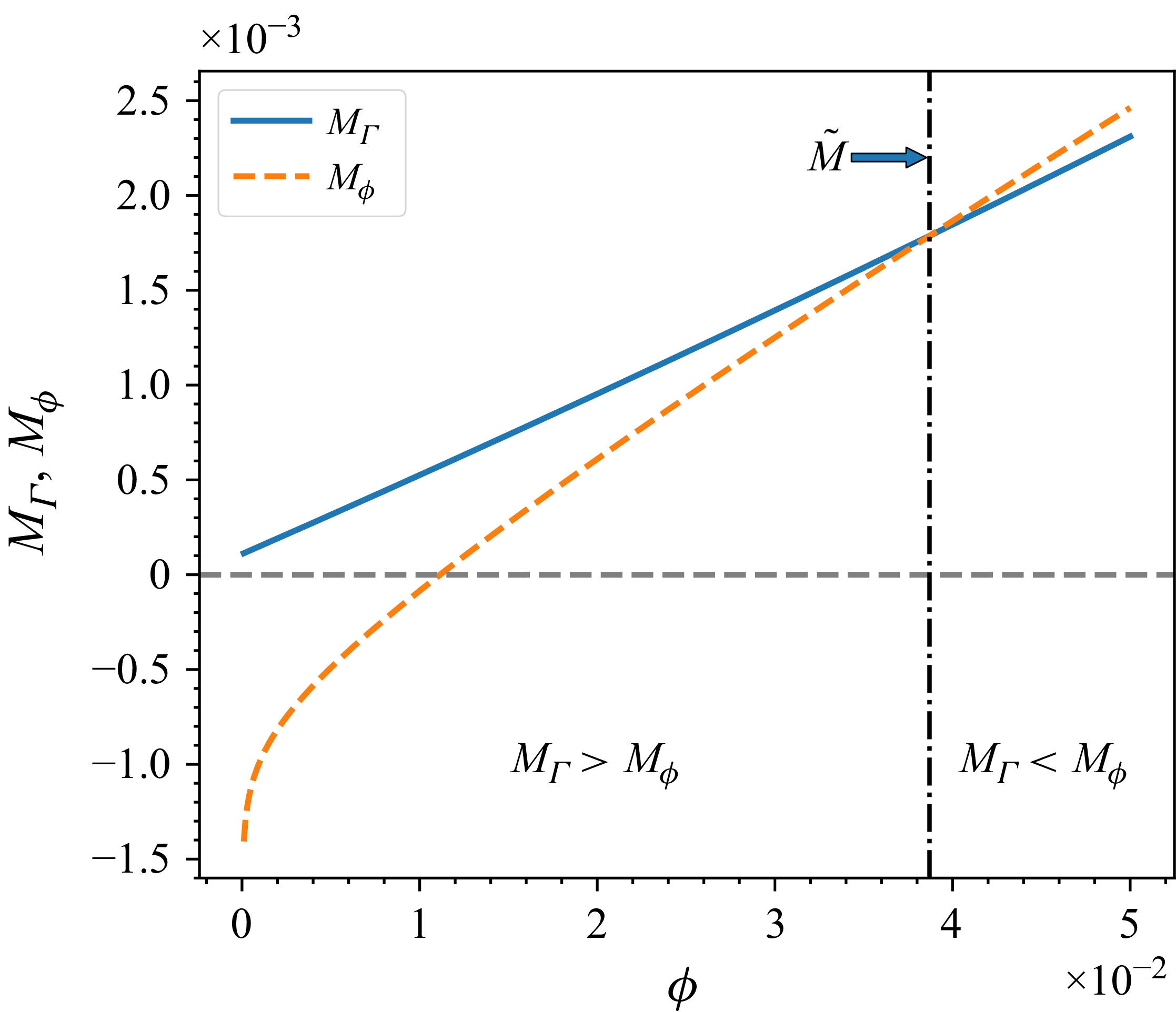


 Open access