2.1. Data description

The United Nations Convention to Combat Desertification in 2017 defined land as “the terrestrial bio-productive system that comprises soil, vegetation, other biota, and the ecological and hydrological processes that operate within the system.” Land degradation describes how one or more of the land resources has changed for the worse. In general, land degradation signifies the temporary or permanent decline in the productive capacity of land, including its major uses (rain-fed, arable, irrigated, rangeland, forest), its farming systems and its value as an economic resource (?).

To carry out the calibration and estimation implemented in this study, we use land data from different sources.Footnote ² Bai et al. (Reference Bai, Dent, Olsson and Schaepman2008) quantify degradation over 1981–2003 by using the normalized difference vegetation index (NDVI) as a proxy for net primary productivity. They find a declining trend in net primary production across 2.7 bn ha (21 per cent) of global land area, but at the same time, they also find that 16 per cent of global land area is increasing in net primary production. We will use their estimates to calibrate some key parameters of the model, but for the empirical exploration we use our own estimates from the EVI. We collect Monthly Moderate resolution Imaging Spectroradiometer (MODIS) data at resolution 0.05 degree (5600 m), from the MODIS data we select the Global MOD13C2 version 6 product, which provides vegetation index values at a per pixel basis. This product provides two vegetation indices: the NDVI and the EVI. In this study we opt for the EVI because it has improved sensitivity over high biomass regions.Footnote ³ The EVI data are monthly data and are available from 2000. As data are at a per pixel basis, the computation of the country's average EVI is time consuming. Therefore, we only collect the MOD13C2 for one month (March) from 2000 to 2015. Afterwards, we import the MODIS data and the country boundaries shapefile into ArcGis and compute the average EVI for each country and year.

The EVI for a given pixel is always a number that ranges from $-1$ to $+1$. Positive values generally indicate the presence of vegetation and negative values generally indicate a lack of vegetation (water, rock, etc.). However, no green leaves gives a value close to zero (a zero means no vegetation) and close to one indicates the highest possible density of green leaves. For instance, the USA's average EVI value over the period 2000–2011 is 0.135 while the average EVI values for the United Kingdom and Spain are 0.332 and 0.267, respectively. We will use a normalization of the EVI data to compute a land quality index as follows: $1-(\max EVI-EVI_{i})$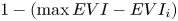, where $\max EVI$ is the maximum value of EVI in our sample which is 0.69 (Samoa) and $EVI_{i}$ is the average value of EVI observed in each country $i$. The physical measure of land adjusted by quality will be the product of this normalized index by the land area. The data on land area are from FAO (land area excluding area under inland water bodies) measured in 1000 ha. We will call this measure of land the “EVI-adjusted land”.

From the World Bank's Wealth of Nations data we obtain estimates of the land-to-output ratios. In this case the value of land is the value of natural capital excluding sub-soil assets. Unfortunately, these estimates are only available for the years 1995, 2000 and 2005, but we will try to get some insights to define our land capital input from the available evidence. The data on income come from the Penn World Table (PWT) in Feenstra et al. (Reference Feenstra, Inklaar and Timmer2015), which cover 182 countries between 1950 and 2014.

The data on pollution abatement efforts to be used in the empirical convergence analysis come from the OECD environmental protection expenditure and revenues dataset and are available for the period 2000-2011 for 35 countries. Finally, data on carbon dioxide emissions are from the World Development Indicators 2016 (World Bank, 2016), which cover 214 countries over the period 1960-2011. These data include gases from the burning of fossil fuels and cement manufacture, but unfortunately exclude emissions from land use and land cover change due to large uncertainties.Footnote ⁴

2.2. Stylized facts

In this section we provide new evidence regarding the EVI-adjusted land, the World Bank's natural capital estimates, and carbon dioxide (CO$_{2}$) emissions. First, we have found a positive significant relationship between the input output ratios of natural capital (excluding sub-soil assets) and the EVI-adjusted land for the available years, 2000 and 2005. Figure 1 shows the positive relationship between these two estimates after controlling for the urban land share effect. It is evident that figure 1 also tells us that there must be other important factors affecting the land capital intensity of economic activity, such as land demand forces stemming from different land uses.Footnote ⁵ We will use this positive relationship as a proxy of the efficiency of land in the production of final goods, meaning that healthier land in a given period is, on average, more valuable and productive. Specifically, we define the variable ‘land capital’ as the product $Z=Q\cdot N,$ where $N$ represents the EVI-adjusted land and $Q$ a technological efficiency factor. Thus, given output, the slopes of the lines in figure 1 can be interpreted as proxies of (proportional to) the average $Q$ for the years 2000 and 2005, respectively. Then, according to this interpretation, the (average world) productivity of land might have decreased over this five-year period. For instance, Amundson et al. (Reference Amundson, Berhe, Hopmans, Olson, Sztein and Sparks2015) show that the ability of soil to support the growth of food supply is plateauing, pointing out that we have the knowledge to recycle soil nutrients but that stronger commitment to implement the solutions is needed.

Figure 1.

Conditional land capital per dollar and EVI-adjusted land per dollar. (a) 2000, (b) 2005. Notes: The land capital per dollar is the value of natural capital excluding sub-soil assets divided by the real GDP at constant 2005 national prices. The EVI-adjusted land per dollar is the product between the normalized vegetation index, $1-(\max EVI - EVI_{i})$, which is between zero and one, and the land area (in 1000 ha) divided by the real GDP at constant 2005 national prices (in mil. 2005US). Figures 1(a) and 1(b) represent the relationship between land capital per dollar and EVI-adjusted land per dollar conditional on the urban land share in the 2000 and 2005, respectively. To remove some outliers, the studentized residuals were calculated and the observations with a residual larger than 3 were removed. The regression in panel (a) has a slope parameter of 0.709 with a standard error of 0.15 and $R^2$ of 0.20. The regression in panel (b) has a slope parameter of 0.608 with a standard error of 0.13 and $R^2$ of 0.17.

Figure 2 illustrates the relationship between the (log) natural capital output and the (log) CO$_{2}$ emissions output ratios for the years 2000 and 2005. It shows that countries with higher natural capital output ratios (higher propensities to save natural capital) are, on average, those with lower emissions per unit of output. Comparing the 2000 and 2005 slopes of this relation, we note that an additional unit of land capital output is associated with a drop in the emissions intensity from 2000 to 2005 of $-0.055$ units. Although data on anthropogenic CO$_{2}$ emissions do not include emissions from the land use and land cover change, we find that there is a statistically-significant relation between the growth of CO$_{2}$ emissions per capita and the growth of EVI-adjusted land per capita. Figure 3 shows that, on average, an increase of one percentage point in the latter is associated with a decrease in the growth rate of emissions per capita of 0.33 percentage points, ceteris paribus.

Figure 2.

CO2 emissions per dollar and land capital per dollar (in logs). (a) 2000, (b) 2005. Notes: To compute the CO2 emissions per dollar, we divide CO2 emissions (in kilotons) by the real GDP at constant 2005 national prices (in mil. 2005US). The land capital per dollar is the value of natural capital excluding sub-soil assets divided by the real GDP at constant 2005 national prices (in mil. 2005US). The left-hand side regression has a slope parameter of -.131 with a standard error of .058 and $R^2$ of 0.05. The right-hand side regression has a slope parameter of -.186 with a standard error of .045 and $R^2$ of 0.13.

Figure 3.

Growth of emissions per capita and growth of EVI-adjusted land per capita. Notes: To compute the CO2 emissions per capita, we divide CO2 emissions (in kilotons) by the population (in millions). The EVI-adjusted land per capita is the product of the normalized vegetation index, which is between zero and one, and the land area (in 1000 ha) divided by the total population (in millions). The growth rates of these two variables are annual growth rates. The corresponding regression has a slope parameter of $-.3349$ with a standard error of $.1673$ and $R^2$ of $0.022$.

Finally, we plot the evolution of CO$_{2}$ output ratios and CO$_{2}$ emissions per capita by income groups. Figure 4 illustrates the evolution of CO$_{2}$ emissions per dollar (emissions per unit of gross domestic product or GDP) over time. The first observation is the declining trend on emissions per dollar for the high income countries in line with the evidence in Brock and Taylor (Reference Brock and Taylor2010). The second observation is that, unfortunately, this fact is not the rule. In a context of technological progress and resource scarcity, emissions per dollar should reflect a downward trend if cleaner and energy-saving technologies are being adopted. In middle income countries the emissions per dollar present a constant positive trend over time and both in low and low-middle income countries the emissions per dollar have in general increased over the last 50 years, which suggests high inefficiencies in production and/or weak growth processes.

Figure 4.

CO2 emissions per dollar by income level. (a) High income, (b) Upper-middle income, (c) Low-middle income, (d) Low income. Notes: To compute the CO2 emissions per dollar, we divide CO2 emissions (in kilotons) by the real GDP at constant 2005 national prices (in mil. 2005US). To classify countries by income group we use the Atlas method used by the World Bank.

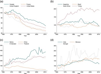
Figure 5 illustrates total CO$_{2}$ emissions for the same groups of countries. We can observe, however, that for the high income countries there is not always a tendency for total carbon emissions to fall. Except for the United Kingdom, showing a downward trend over the whole period, high income countries show something like an inverted-U relationship (an EKC) over time. France and the United States follow similar upward trends until the beginning of the eighties, but only France shows a clear downward trend afterwards. Total emissions in the United States and Canada show a very marked upward trend until 2008 and then start to decline, though Canada registers the highest growth in total emissions over the whole period.

Figure 5.

Total CO2 emissions by income level. (a) High income, (b) Upper-middle income, (c) Low-middle income, (d) Low income. Notes: Total CO2 emissions in kilotons. To classify countries by income group we use the Atlas method used by the World Bank.

3.1. Adding land capital to the Green Solow model

The level of economic activity is represented by an aggregate production function, $F( K,Z,BL)$, satisfying the standard neoclassical properties. In this function, $K$ represents manufactured capital, $Z$ is land capital, $L$ is labor, and $B$ is a labor-augmenting technology parameter that grows exogenously at the rate $g_{B}$. We assume that the labor supply of the economy is equal to the population size and that population grows at the rate $g_{L}$, which is also exogenous. For simplicity, and since we are interested in finding convenient closed-form solutions for the empirical analysis, we assume that $F$ is a Cobb-Douglas production function,

(1)\begin{equation} F\left( K,Z,BL\right) =K^{\alpha }Z^{\beta }\left( BL\right) ^{1-\alpha -\beta }\ with\ \alpha ,\beta \in \left( 0,1\right).\end{equation}

Land capital, $Z=Q\cdot N,$ is an environmental asset that results from the combination of environmental knowledge, $Q$, and a quality (EVI-adjusted) land area, $N.$ Environmental knowledge is the result of learning and adapting the existing knowledge to land services, which is costly.Footnote ⁶ Thus, given a fixed land area, land productivity is captured by the product of the biological index (normalized EVI) and the knowledge factor, which is modelled just as a land-augmenting efficiency factor.Footnote ⁷ The definition of land capital is related to the soil input in Braussman and Bretscheger (Reference Braussman and Bretscheger2018), where the quality and quantity aspects of soil are important. In that model, soil investments include both investment effort to increase productivity and land clearing to increase quantity, but they only study aggregate investment in an integrated manufactured capital-soil asset. Here, we treat land in a broad sense, including all land resources (not only soil) and consider land capital investment and manufactured capital investment separately. Nevertheless, the mechanism by which the productivity of the natural input can be improved is the same as in Braussman and Bretscheger (Reference Braussman and Bretscheger2018); the rise in productivity is driven by the amount of environmental investment. We assume that the resulting environmental knowledge is proportional to the amount spent on environmental investment, $I_{z},$ per unit of land. Taking into account the depreciation of knowledge, which occurs at the rate $\delta _{Q}$, the net environmental productivity gains are

(2)\begin{equation} \overset{\cdot }{Q}=\upsilon \frac{I_{z}}{N}-\delta _{Q}Q,\quad 0<\upsilon \leq 1. \end{equation}

In addition, the economic activity generates a negative production externality on land quality, which is assumed to be proportional to the land capital intensity of economic activity, $\Psi \frac {F}{Z}$, where $\Psi$ is a constant externality parameter. This externality includes, for example, land damage from industrial residuals, inadequate management of households’ residuals and harmful soil management practices. With this specification, given output and land endowment, larger stocks of environmental knowledge tend to alleviate the effect of production on land degradation. We follow Braussman and Bretscheger (Reference Braussman and Bretscheger2018) and assume that the economy's efforts in protection and abatement activities decrease the human-induced damage on land quality. We define the net damage as $( \Psi F-\Psi P) /Z$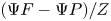, where protection $P$ is a strictly concave constant returns to scale function of total output and the economy's protection efforts, $P( F,\theta F)$, with $\theta$ being the fraction of output spent on protection and abatement activities. Then, we can write the evolution of the quality (EVI)-land $N$ as

(3)\begin{align} \overset{\cdot }{N} & ={-}\mu \left( K,Z\right) N, \end{align}

(4)\begin{align} \mu \left( K,Z\right) & :=\delta _{N}-\eta +\Psi p\left( \theta \right)\frac{F}{Z},\quad p\left( \theta \right) =1-P\left( 1,\theta \right) , \end{align}

where the function $\mu$ represents the overall rate of land degradation; $\delta _{N}-\eta$ is the exogenous rate of land depreciation upon use in production net of natural regeneration; $P( 1,\theta )$ represents total protection per unit of output; and so $\Psi p( \theta )$ is net damage per unit of output. Then, taking into account (2), (3) and (4), the evolution of $Z$ can be written as

(5)\begin{equation} \overset{\cdot }{Z}=\upsilon I_{Z}-\delta _{Z}Z-\Psi p\left( \theta \right) F\left( K,Z,BL\right) ,\quad \delta _{Z}=\delta _{Q}+\delta _{N}-\eta.\end{equation}

In this framework, gross output net of protection and abatement expenditures, $( 1-\theta ) F$, will be allocated to consumption, $C$, environmental investment, $I_{Z}$, and manufactured capital investment, $I_{K}$. So, given a constant rate of depreciation of manufactured capital, $\delta _{K}$, we can write the evolution of $K$ as

(6)\begin{equation} \overset{\cdot }{K}=\left( 1-\theta \right) F\left( K,Z,BL\right) -C-I_{z}-\delta _{K}K. \end{equation}

Let $s_{K}$ and $s_{Z}$ be the exogenous investment rates of manufactured capital and land capital out of $( 1-\theta ) F$, respectively. Then, transforming the measures of output, manufactured capital and land capital into intensive units, and defining the normalized variable of $X$ as $x\equiv X/BL,$ capital accumulation in the extended Green Solow model with land degradation is given by

(7)\begin{align} \frac{\overset{\cdot }{k}}{k} & = s_{K}\left( 1-\theta \right) \frac{f\left( k,z\right) }{k}-\left( \delta _{K}+g_{B}+g_{L}\right) , \end{align}

(8)\begin{align} \frac{\overset{\cdot }{z}}{z} & =\left[ \upsilon s_{Z}\left( 1-\theta \right) -\Psi p\left( \theta \right) \right] \frac{f\left( k,z\right) }{z} -\left( \delta _{Z}+g_{B}+g_{L}\right) . \end{align}

3.1.1. Balanced growth in the extended Green Solow model

A Balanced Growth (BG) solution to manufactured capital and land capital accumulation is a stationary solution $( k^{\ast },z^{\ast })$ to the above system, where $K$, $Z$ and $F$ will grow at the rate $g_{B}+g_{L},$ and the corresponding per capita variables at the rate $g_{B}.$ This solution exists and it is unique as long as $\upsilon s_{Z}( 1-\theta ) -\Psi p( \theta ) >0$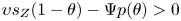, that is, that the economy's efforts at investing and protecting land capital are sufficient to counter land degradation. Under this condition, the economy converges to $( k^{\ast },z^{\ast })$ for any given $k( 0) >0,$ $z( 0) >0.$ The corresponding capital output ratios and the BG solution are, respectively:

(9)\begin{align} \frac{k^{{\ast} }}{f\left( k^{{\ast} },z^{{\ast} }\right) } & =\frac{s_{K}\left( 1-\theta \right) }{\left( \delta _{K}+g_{B}+g_{L}\right) }, \end{align}

(10)\begin{align} \frac{z^{{\ast} }}{f\left( k^{{\ast} },z^{{\ast} }\right) } & =\frac{\upsilon s_{Z}\left( 1-\theta \right) -\Psi p\left( \theta \right) }{\left( \delta _{Z}+g_{B}+g_{L}\right) }, \end{align}

(11)\begin{align} k^{{\ast} } & =\left( \frac{s_{K}\left( 1-\theta \right) }{\delta _{K}+g_{B}+g_{L}}\right) ^{\frac{1-\beta }{1-\alpha -\beta }}\left( \frac{ \upsilon s_{Z}\left( 1-\theta \right) -\Psi p\left( \theta \right) }{\delta _{Z}+g_{B}+g_{L}}\right) ^{\frac{\beta }{1-\alpha -\beta }} \end{align}

(12)\begin{align} z^{{\ast} } & =\left( \frac{s_{K}\left( 1-\theta \right) }{\delta _{K}+g_{B}+g_{L}}\right) ^{\frac{\alpha }{1-\alpha -\beta }}\left( \frac{ \upsilon s_{Z}\left(1-\theta \right) -\Psi p\left( \theta \right) }{\delta _{Z}+g_{B}+g_{L}}\right) ^{\frac{1-\alpha }{1-\alpha -\beta }}. \end{align}

To close the Green Solow model, we have to add the emissions externality equation. As in Brock and Taylor (Reference Brock and Taylor2010), we assume that each unit of output generates $\Omega$ units of pollution that can be in part reduced by the economy's efforts at abatement. The emissions abatement function is a concave constant returns to scale function of output and the economy's abatement effort, $A( F,\theta ^{a}F)$, where $\theta ^{a}$ is the fraction of output spent specifically on air emissions abatement. So the level of emissions released into the atmosphere is $E=( 1-A( 1,\theta ^{a}) ) \Omega F( K,Z,BL) ,$ or in terms of the normalized variables:

(13)\begin{equation} e=a\left( \theta ^{a}\right) \Omega f\left( k,z\right) ,\quad a\left( \theta ^{a}\right) \equiv 1-A\left( 1,\theta ^{a}\right) , \end{equation}

where it is assumed that each period technological progress in abatement makes the intensity of emissions, $\Omega$, fall at the exogenous rate $g_{A}.$ To this setting we add a link between the growth rate of emissions and the change in land capital intensity of economic activity, trying to incorporate the facts illustrated in figures 2 and 3. Specifically, taking into account equation (4), we assume that

(14)\begin{equation} \overset{\cdot }{\Omega }=\Omega \left[{-}g_{A}+\zeta \cdot \left( \frac{ \overset{\cdot }{F}}{F}-\frac{\overset{\cdot }{Z}}{Z}\right) \right] ,\;\zeta >0, \end{equation}

where the parameter $\zeta$ captures the sensitivity of emissions intensity to the change in the land degradation rate. We call this parameter the environmental stress parameter. Since environmental stress appears when the demand or use of a natural factor grows faster than its natural supply, land degradation is a form of environmental stress. Assuming that the growth rate of demand for natural capital services is proportional to the growth rate of economic activity, the difference between the growth rate of output and the growth rate of natural capital supply will capture the extent of this environmental stress. However, note that along the BG solution, total output and total capital output will grow at the same rate, so

(15)\begin{equation} g_{E}^{{\ast} }=\frac{\overset{\cdot }{\Omega }}{\Omega }+\frac{\overset{\cdot }{F}}{F}={-}g_{A}+g_{B}+g_{L}. \end{equation}

Therefore, the long-run air quality condition, $g_{E}^{\ast }<0,$ and sustained output growth, $g_{B}>0$, will imply the same sustainability restrictions as in Brock and Taylor (Reference Brock and Taylor2010):

(16)\begin{equation} g_{B}+g_{L}< g_{A},\;g_{B}>0. \end{equation}

3.2. Parameter values

In this subsection we discuss the numerical values that will be assigned to some technology and environmental parameters, which will be assumed to be the same across countries in the empirical analysis, and compute the investment rates implied by the model. We take the US economy as the reference for most of the parameters, assuming that it is on its balanced growth path.

The US average growth rates of population and income per capita over the last 30 years are $1$ per cent and $2$ per cent, respectively. So the estimated rate of technological progress is also $2$ per cent, $g_{B}=0.02$. The factor shares of total output in the Cobb-Douglas technology can be calibrated using the respective factor income shares of total GDP. The problem we face here is that the natural factor comprises the value of services that do not always have a market value. We will rely on the World Bank's estimates provided in “Changing wealth of nations, measuring sustainable development in the new millennium” (World Bank, 2011, table 5.4), where the elasticities of output for all countries with respect to natural capital and produced capital are $0.068$ and $0.32$, respectively. These values are similar to the land and capital income shares estimated by Valentinyi and Herrendof (Reference Valentinyi and Herrendof2008) from the USA input-output dataset, which are $0.05$ and $0.33$, respectively. The ratios of land capital and manufactured capital to output can be calculated from the World Bank data available for the years 1995, 2000 and 2005. These data imply an average value of produced capital to gross national income equal to $2.27$, and an average value of natural capital excluding sub-soil assets (crop land, pasture land, forest land and protected areas) to gross output equal to $0.29.$

With respect to the depreciation rate of manufactured capital, we can set $\delta _{K}=0.1$, a frequent value in global economy models (e.g., Lanz et al., Reference Lanz, Dietz and Swanson2017a; Hwang et al., Reference Hwang, Tol and Hofkes2019), or $\delta _{K}=0.05$, a standard value in the growth literature.Footnote ⁸ However, we do not have standard values for the depreciation of land. To assign values to $( \delta _{N}-\eta )$ and $\mu$ in equation (4), we will assume that the former corresponds to the part of land degradation that is directly due to agricultural activities. Based on the NDVI, Bai et al. (Reference Bai, Dent, Olsson and Schaepman2008) estimate that the degrading land for the USA over $1981-2003$ accounted for $20.6$ per cent of total land area, which would imply an annual average degrading rate of $1$ per cent over that period given that significant human-induced land degradation started 200 years ago. Assuming $\ 23$ per cent of total degraded area is due to agricultural activities, this would imply an annual depreciation rate due to agriculture of around $0.18$ per cent.Footnote ⁹ In summary, we fix $\mu ^{\ast }=0.01$ and $( \delta _{N}-\eta ) =0.0018$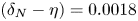.Footnote ¹⁰ With these values, we can use equation (4) and the land capital output ratio set above, $z/f=0.29$, to get an estimate for the net human-induced damage factor, $\Psi p( \theta ) =0.0024.$ 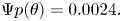Under a situation of zero protection effort, this equation would imply a damage parameter of $\Psi =0.0024.$ Finally, regarding land capital depreciation, we consider a depreciation rate of environmental research equal to $\delta _{Q}=0.1,$ as in the active learning approach of Hwang et al. (Reference Hwang, Tol and Hofkes2019).

The enacted budgets of the Environmental Protection Agency (EPA) yield an average agency budget share of GDP around $0.058$ per cent per year over $1998-2018$, with a maximum $0.08$ per cent share in $1998$ and around $0.04$ per cent since $2014$. Data from the US Department of Agriculture (USDA) budget outlays report spending shares of natural resources conservation service and wildland fire management that add up to $0.02$ per cent every year over $2006-2015.$ With respect to pollution abatement costs, Brock and Taylor (Reference Brock and Taylor2010) report a GDP share of $1.6$ per cent, or $0.5$ per cent if abatement costs refer specifically to air pollutants. Altogether, these estimates suggest an average protection and abatement expenditure share $\theta$ of GDP around $1.68$ per cent.

Taking into account these parameter values, we use equations (9 ) and (10) to compute the implied investment rates of the model. The investment rate for manufactured capital is $18$ or $30$ per cent depending on whether the depreciation rate considered is $5$ or $10$ per cent, respectively, which is consistent with average historical values of the USA economy of around 20 per cent. In contrast, the implied investment rate for land capital hinges on the conversion factor of environmental investment, $0.04/\upsilon,$ and we do not have systematic historical data to compare with. The environmental research spending that we have found for the USA economy (which for other countries is even worse) refers to the USDA annual spending on Agricultural, Forest and Rangeland research services over $2006-2015$ and to the EPA annual spending in Science and Technology over $2010-2018.$ They yield annual average GDP shares of $0.0098$ and $0.004$ per cent, respectively. Altogether these values would imply an environmental investment rate of $\ 0.014$ per cent, which assuming a very optimistic conversion factor $\upsilon =1,$ would clearly be well below the $4$ per cent investment rate implied by the model. Note that this parameter captures the conversion of foregone consumption (or manufactured capital) to environmental knowledge, and so it is a key parameter, together with $\Psi$ in the tradeoff between land protection and land investment efforts.

Finally, we assign values to $\zeta$ (the environmental stress parameter of emissions) and $g_{A}$ (the rate of technological progress in air emissions abatement). Figure 2 implies that the estimated change in emissions intensity from $2000$ to $2005$ due to an additional unit of land capital output ratio is, on average, $-0.055.$ So we fix the environmental stress parameter (partial effect of the change in the output land capital ratio on the change of emissions intensity in equation (14)) to $\zeta =0.055.$ With respect to the rate of technological progress in air emissions abatement, first we note that since emissions per capita have been falling at an average rate of $-0.6$ per cent per year and population has been rising at an average rate of $1$ per cent per year, the growth rate of total emissions is positive in the USA economy. In other words, these data do not satisfy the sustainability condition in emissions, $g_{E}^{\ast }<0.$ Note that equation (15) would imply that $g_{A}=g_{B}+g_{L}-g_{E}^{\ast }=0.026,$ thus, violating the condition that requires long-run sustainability, $g_{A}>0.03$.

Table 1 summarizes the calibrated parameters. The empirical tests in the regression analysis will confirm that most of these parameter values are reasonable.

Table 1.

Calibrated parameters

4.1. Econometric specification

In this section we derive the estimating equation and estimate the model using the data described in section 2.1. Our purpose is to explore how the EVI-adjusted land input, economic activity and actual environmental policies affect the growth of emissions per capita. To do that, we rewrite equation ( 13) in per capita terms,

\[ e^{c}=\frac{a\left( \theta ^{a}\right) }{1-\theta }\Omega y^{c}, \]

where $x^{c}$ is variable $x$ in per capita terms. Differentiating with respect to time and taking into account expression (14), we obtain the growth rate of emissions per capita,

(17)\begin{equation} \frac{\overset{\cdot }{e^{c}}}{e^{c}}={-}g_{A}+\left( 1+\zeta \right) \frac{ \overset{\cdot }{y^{c}}}{y^{c}}-\zeta \frac{\overset{\cdot }{z^{c}}}{z^{c}}.\end{equation}

As our data is discrete and we are interested in a time horizon of size T, we follow the approach in Mankiw et al. (Reference Mankiw, Romer and Weil1992) and Brock and Taylor (Reference Brock and Taylor2010), approximating the continuous growth rates of emissions per capita and income per capita by their log changes, and the growth rate over a given period by the average of log changes:

(18)\begin{equation} \frac{1}{T}\ln \left( \frac{e_{t}^{c}}{e_{t-T}^{c}}\right) ={-}g_{A}+\left( 1+\zeta \right) \frac{1}{T}\ln \left( \frac{y_{t}^{c}}{y_{t-T}^{c}}\right) -\zeta \frac{1}{T}\ln \left( \frac{z_{t}^{c}}{z_{t-T}^{c}}\right) .\end{equation}

Next, following the standard approach we log-linearize the growth of income per capita and land capital per capita around the model's steady state:Footnote ¹¹

(19)\begin{align} \ln \left(\frac{y_{t}^c}{y_{t-T}^c} \right) & = \big(1-\exp\left(-\gamma_{y} T\right)\big) \ln (y^{c*}) - \big(1-\exp \left(-\gamma_{y} T\right)\big)\ln(y_{t-T}^c), \end{align}

(20)\begin{align} \ln \left(\frac{z_{t}^c}{z_{t-T}^c} \right) & = \big(1-\exp\left(-\gamma_{z} T\right)\big) \ln (z^{c*}) - \big(1-\exp \left(-\gamma_{z} T\right)\big)\ln(z_{t-T}^c), \end{align}

where $\gamma _{y}$ and $\gamma _{z}$ denote the long-run convergence rates of $y$ and $z$, given by $\gamma _{y}\approx ( 1-\alpha -\beta ) (\delta +g_{B}+g_{L})$ and $\gamma _{z}\approx ( 1-\beta ) ( \delta +g_{B}+g_{L})$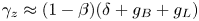, respectively. Substituting $y^{c\ast }=( 1-\theta ) Bk^{\ast ^{\alpha }}z^{\ast ^{\beta }}$ 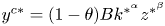into equation (19) and using equation (17) to get $y_{t-T}^{c}=\frac {( 1-\theta ) e_{t-T}^{c}}{a(\theta )\Omega _{t-T}}$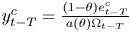, we can rewrite (18) and obtain the estimating equation:

(21)\begin{align} \frac{1}{T}\ln \frac{e_{it}^{c}}{e_{it-T}^{c}}& = \rho _{0}+\rho _{1}\ln e_{it-T}^{c}+\rho _{2}\ln z_{it-T}^{c}+\rho _{3}\ln s_{k_{i}} +\rho _{4}\ln (\upsilon s_{Z_{i}}(1-\theta _{i}) \notag\\ & \quad -p\left( \theta _{i}\right) \Psi _{i})+ \rho _{5}\ln \left( 1-\theta _{i}\right) +\rho _{6}\ln \left( \delta +g_{B}+g_{L}\right) _{i}+\nu _{i}, \nonumber\\ \rho _{0}& = g_{B}-g_{A}+(1+\zeta )\Big[\frac{\big(1-exp\left( -\gamma _{y}T\right) \big)}{T}\ln \Omega _{t-T}B_{t-T}\Big] \nonumber\\ \rho {1}& ={-}\left( 1+\zeta \right) \frac{\left( 1-exp\left( -\gamma _{y}T\right) \right) }{T} \nonumber\\ \rho _{2}& = \zeta \frac{\left( 1-exp\left( -\gamma _{z}T\right) \right) }{T} \nonumber\\ \rho _{3}=& \frac{\alpha }{1-\alpha -\beta }\Big[(1+\zeta )\frac{\big( 1-exp\left( -\gamma _{y}T\right) \big)}{T}-\zeta \frac{\big(1-exp\left( -\gamma _{z}T\right) \big)}{T}\Big] \nonumber\\ \rho _{4}=& \Big[(1+\zeta )\frac{\beta }{1-\alpha -\beta }\frac{\big( 1-exp\left( -\gamma _{y}T\right) \big)}{T}-\zeta \frac{1-\alpha }{1-\alpha -\beta }\frac{\big(1-exp\left( -\gamma _{z}T\right) \big)}{T}\Big] \nonumber\\ \rho _{5}=& \Big[(1+\zeta )(\epsilon -1+\frac{1-\beta }{1-\alpha -\beta }) \frac{\big(1-exp\left( -\gamma _{y}T\right) \big)}{T} \notag \\ & \qquad -\zeta \frac{\alpha }{ 1-\alpha -\beta }\frac{\big(1-exp\left( -\gamma _{z}T\right) \big)}{T}\Big]\end{align}

(22)\begin{align} \rho _{6}=& -\Big[(1+\zeta )\frac{\beta }{1-\alpha -\beta }\frac{\big( 1-exp\left( -\gamma _{y}T\right) \big)}{T} \notag \\ & \qquad -\zeta \frac{1-\alpha }{1-\alpha -\beta }\frac{\big(1-exp\left( -\gamma _{z}T\right) \big)}{T}\Big]. \end{align}

Thus, the average change in emissions per capita over a period of length $T$ is determined by the initial value of emissions per capita, $e_{t-T}^{c}$, the initial value of land capital per capita, $z_{t-T}^{c}$, and a set of variables that capture the effect of income per capita in the long run. These variables are the manufactured capital investment rate, $s_{k}$; the land capital investment rate, $s_{z}$; the abatement effort, $\theta$; the human-induced damage, $\Psi$; and the depreciation term, $( \delta +g_{B}+g_{L})$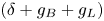, which depends on the depreciation rate of capital ($\delta =\delta _{k}=\delta _{z}$), the rate of labor-augmenting technological progress, $g_{B}$, and the rate of population growth, $g_{L}$.

4.2. Empirical results

Data used in the econometric analysis were described in sections 2 and 3.2. To summarize briefly, for emissions we consider data on CO$_{2}$ in kilotons (kt) from the World Development Indicators 2016. For data on population, GDP and GDP share of manufactured capital investment, we collect data from the Penn World Table. Data on abatement efforts come from the OECD, and data related to land capital come from different sources: natural capital excluding sub-soil assets from the World Bank, land area from FAO, and EVI data from the NASA Earth Observatory.

The time period under analysis is 2000–2011. Recall that land capital in the model is defined as $Z=Q\ast EVI\ast \overline {N}$, and that data on this asset is only available from the World Bank for a few years. We proxy $Z$ by the EVI-adjusted land variable and the land capital investment term by the World Bank capital output ratio estimates. By doing this, first note that the constant term in equation (21) will include an additional term proportional to $\ln Q_{t-T}$. Second, using the land capital output data and the calibrated values of $\delta _{Z}=0.1$, $g_{B}=0.02$ and $g_{L}=0.01$, we obtain from equation (9) the country values of the variable $\upsilon s_{Z}(1-\theta )-p( \theta ) \Psi$ to be used in the estimation of (21). It is worth mentioning that $s_{z}{}_{i},$ $s_{k}{}_{i}$, $\theta _{i}$ and $( \delta +g_{B}+g_{L}) _{i}$ 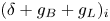are time-average country specific. Moreover, we follow Brock and Taylor (Reference Brock and Taylor2010) and set the abatement technology factor as $a(\theta ^{a})=(1-\theta ^{a})^{\varepsilon }$, with $\varepsilon >1$. As the abatement intensity for carbon is close to zero, we set $\theta ^{a}=0.005$ for every country.

Finally, regarding the variable $(\delta +g_{B}+g_{L})$, we use the population data to find the population growth over the period 2000–2011, and use the calibrated values of $\delta _{k}=0.1$ and $g_{B}=0.02$. Thus, this term captures only the variation in population growth rates across countries. The study covers 146 countries; the country sample is limited by the availability of data in the Penn World Table.

To estimate the model, we follow Barro (Reference Barro1991), Durlauf and Johnson (Reference Durlauf and Johnson1995), Brock and Taylor (Reference Brock and Taylor2010), and others, and employ the heteroskedasticity-corrected standard error estimates. The estimation results are presented in table 2 and the empirical tests presented have to be interpreted as a test of the devised model.Footnote ¹² Column A presents the unconditional convergence results, column B reports the results for the shorter specification of the model (controlling only for the initial value of land capital) and columns C-E report the results for the longer specification of the model. Columns A-C include all countries in our sample while columns D and E only include the upper-middle income and the low income countries, respectively.Footnote ¹³

Table 2.

Estimated model results for CO2 emissions per capita growth rates

Notes: Standard errors are in parentheses. Columns (A) and (B) estimate the short version of our model described in (21) and the remaining columns estimate the longer version of the model. Columns (A)-(C) include all countries in the sample while Columns (D) and (E) only include the upper-middle income and the low income countries, respectively. Column (C) is the preferred model. The dependent variable is the average growth rate in log emissions per capita over the 2000–2011 period, $e_{t-T}^c$ is the emissions per capita in 2000, $z_{t-T}^c$ is the land capital per capita in 2000 (proxied by the EVI-adjusted land per capita), the $s_{k}$ is the average capital investment to GDP ratio over the 2000–2011 period, $(\delta +g_{B}+g_{L})$ is the average population growth over the period where $\delta$ is set equal to 0.1, $g_{B}$ is set equal to 0.02 and $s_{z}$ represents the land capital investment rate net of land degradation (proxied by the average land capital output ratio).

The Green Solow model with land capital explains quite well the cross-country variation in the growth rates of CO$_{2}$ emissions per capita over the period 2000–2011. The short version of the empirical model (column B) shows that the negative coefficient of the initial emissions per capita, $\ln e_{t-T}^{c}$, and the positive coefficient of the initial quality-adjusted land per capita, $\ln z_{t-T}^{c}$, are both statistically significant. These results are confirmed by the longer version of the model in column C, which is our preferred model, and by the subsequent restricted country samples (columns D and E). Not surprisingly, the explanatory power of the long version of the model is greater than that of the short version, explaining approximately $24$ per cent of the variation of the per capita carbon emissions growth rates over the period.

The empirical results imply that, given control variables, an equal proportional increase in initial emissions and land capital would reduce the growth rate of emissions per capita (columns B (short version) and C (long version)). That is, the net convergence effect (i.e., the combined impact from initial per capita values of emissions and land capital on the growth rate of emissions per capita) is negative and statistically significant. Moreover, the speed of convergence (i.e., the reaction of the growth rate of emissions to the initial emissions level) is greater in the long version of the model despite the higher influence of the initial EVI-adjusted land endowment. In the short version of the model (column B), the speed of convergence is slightly lower than in the unconditional convergence case (column A), implying that the omission of the natural endowment might be behind the convergence results in some empirical studies. In the long version of the model (column C), however, the speed of convergence more than doubles the unconditional rate of the shorter version (column B). Figure 6 plots the absolute and conditional convergence results for the whole country sample (columns A, B and C). In other words, if there were identical parameter values across countries (same steady states), the model would predict absolute convergence in emissions per capita but at a slower speed for countries with better initial endowments of EVI-adjusted land.

Figure 6.

Unconditional and conditional convergence. (a) Unconditional convergence, (b) Conditional convergence, (c) Conditional convergence. Notes: Panel (a) plots the growth of emissions per capita against the initial emissions per capita. Panel (b) plots the growth of emissions per capita against the initial emissions per capita conditional on the initial adjusted land quality. Panel (c) plots the the growth of emissions per capita against the initial emissions per capita conditional on the initial EVI-adjusted land per capita, the average capital investment share $(s_{k})$, the population growth rate, $(\delta +g_{B}+g_{L})$, and the land capital investment rate net of land degradation $(\upsilon s_{z}(1-\theta )-\Psi p( \theta ) )$.

A positive and statistically-significant coefficient of the initial EVI-adjusted land means that the implied environmental stress parameter $\zeta$ is positive in all estimations (see definition of $\rho _{2}$ in equation (22)), which is in accordance with the theoretical prediction of the model. Everything else constant, a lower initial value of land capital means a higher growth rate of $z$ and so a lower growth rate of emissions (see equation (14)). This is a direct negative effect of the growth rate of land capital on the growth rate of emissions. But the theoretical model also establishes an indirect positive effect that goes through the growth of final output; that is, lower initial levels of land capital are associated with lower initial levels of output and so higher growth rates of output and emissions along the transition path. What the empirical result tells us about the role of the initial EVI-adjusted land endowment is that the direct effect dominates. In contrast, the coefficient of the land capital investment rate is negative (statistically significant in all specifications of the model except for the low income country subsample, column D). This coefficient captures the overall long-run effect of land capital intensity on the growth rate of emissions per capita. A higher land capital output ratio means faster land capital growth relative to output growth and a lower emissions intensity. Note that this effect is driven by the effectiveness of technological progress in abatement (equation (11)); without this collateral effect, a higher land capital investment rate would just increase both long-run output and emissions. Thus, the model predicts that the overall effect of investment can slow down the growth rate of emissions per capita through higher investment rates in land capital. No doubt there are other plausible theoretical interpretations arising from alternative frameworks, but the estimates in table 2 have to be interpreted as a test of the extended Green Solow model with land capital.Footnote ¹⁴

Also in accordance with the predictions of the theoretical model, the manufactured capital investment rate has a positive and statistically-significant effect on the growth rate of CO$_{2}$ emissions per capita (not statistically significant in the upper-middle income subsample, column D). The population growth effect is not in accordance with Brock and Taylor (Reference Brock and Taylor2010) results (negative or not significant); here it is positive and statistically significant only for the restricted sample of upper-middle income countries. A possible interpretation of this result is that upper-middle income countries are those undergoing faster degradation due to structural changes and greater population pressure.

These convergence results should be interpreted with caution due to the limited time horizon considered. Nevertheless, they shed light on the mixed evidence about convergence of CO$_{2}$ emissions across countries, pointing to the need to account for specific structural characteristics such as climate or natural resources (see Pettersson et al., Reference Pettersson, Maddison, Acar and Soderholm2014 for a review of the literature). Therefore, better international data on environmental services is a prerequisite for more profound analysis of the emissions convergence issue. Another prerequisite, as already mentioned, is better data on emissions from land use and land cover change at the country or regional level.

Despite the data limitations, the implied values for the key parameters of the model, $\zeta$ and $\beta,$ are very close to the calibrated values reported in table 1. Specifically, using the estimated coefficients of the general case (column B) and equations in (22), the imputed values are $\zeta =0.065$ and $\beta =0.051$. In contrast, the implied GDP share of manufactured capital, $\alpha =0.697$, and the speed of convergence of income per capita, $\gamma _{y}=0.02$, are too large and too low, respectively, compared to reasonable theoretical values, but similar to those reported in Brock and Taylor (Reference Brock and Taylor2010) and other related empirical work (see, for example, Barro and Sala-i-Martin (Reference Barro and Sala-i-Martin2004), chapter 12).