


1. Introduction
Malaria, a vector-borne disease transmitted to humans through the bite of an infected female Anopheles mosquito, remains a significant public health challenge, affecting nearly half of the global population. In 2022, malaria caused 249 million infections and 608,000 deaths worldwide, with 95% of the burden concentrated in sub-Saharan Africa [37]. To mitigate the impact of malaria, global initiatives have focused on vector control measures, which significantly reduced the disease burden in Africa between 2005 and 2015 [Reference Bhatt, Weiss, Cameron, Bisanzio, Mappin, Dalrymple, Battle, Moyes, Henry, Eckhoff, Wenger, Briët, Penny, Smith, Bennett, Yukich, Eisele, Griffin, Fergus, Lynch, Lindgren, Cohen, Murray, Smith, Hay, Cibulskis and Gething7, Reference Thomas and Read44]. This success was largely driven by widespread use of pyrethroid-based insecticides and indoor residual spraying (IRS), with pyrethroid-treated nets (ITNs) playing a pivotal role due to their low toxicity to mammals and strong irritant effects on mosquitoes [Reference Alout, Roche, Dabiré, Cohuet and Knoll2, Reference Thomas and Read44].
However, these gains are now under threat due to the rapid emergence of insecticide resistance in mosquito populations. Prolonged insecticide use exerts selection pressure, allowing mosquitoes to survive and reproduce despite exposure to chemical agents such as pyrethroids [Reference Alout, Roche, Dabiré, Cohuet and Knoll2, Reference Hemingway, Ranson, Magill, Kolaczinski, Fornadel, Gimnig, Coetzee, Simard, Roch, Hinzoumbe, Pickett, Schellenberg, Gething, Hoppé and Hamon21, 36]. Since long-lasting insecticidal nets (LLINs) form the cornerstone of malaria eradication strategies, resistance in Anopheles mosquitoes presents a critical challenge to public health efforts in sub-Saharan Africa [35]. Resistance arises as exposure to insecticides selects genetic mutations that confer survival advantages, enabling the spread of resistance genes in mosquito populations (e.g. [Reference Adams, Selland, Willett, Carew, Vidoudez, Singh, Catteruccia and McGraw1, Reference Hamid-Adiamoh, Amambua-Ngwa, Nwakanma, D’Alessandro, Awandare and Afrane19, Reference Machani, Ochomo, Zhong, Zhou, Wang, Githeko, Yan and Afrane26]). Understanding the evolutionary dynamics underlying the emergence and spread of mosquito insecticide resistance is therefore essential for developing sustainable management strategies.
Mathematical modelling has long been a valuable tool for understanding the complex dynamics of biological systems with nonlocal terms and structured populations, particularly in epidemiology (e.g. [Reference Bentout5, Reference Bentout6, Reference Djidjou-Demasse, Ducrot and Fabre13, Reference Pane, Richard, Seydi and Djidjou-Demasse38]). In the context of vector-borne diseases, mathematical models have played a key role in elucidating how mosquito population dynamics influence disease transmission. More recently, models incorporating population genetics have been developed to investigate the community-level consequences of insecticide resistance in mosquito populations [Reference Barbosa and Hastings3, Reference Barbosa, Kay, Chitnis and Hastings4, Reference Birget and Koella8, Reference Hobbs, Weetman and Hastings22, Reference Kuniyoshi and dos Santos24, Reference Levick, South, Hastings and Pascual25, Reference Madgwick and Kanitz27, Reference Mohammed-Awel and Gumel33, Reference Mohammed-Awel and Gumel34, Reference Sudo, Takahashi, Andow, Suzuki and Yamanaka40]. These models typically address qualitative resistance by examining the dynamics of specific resistance alleles – homozygous sensitive (SS), heterozygous (RS) and homozygous resistant (RR) – and their interactions within the population. While these approaches provide valuable insights into the genetic basis and spread of resistance, they often overlook the transient evolutionary dynamics that contribute to its emergence.
In cases where resistance is driven by point mutations, mosquito insecticide resistance can be viewed as a continuous trait, referred to as quantitative insecticide resistance. This form of resistance arises from the combined effects of multiple genes, each contributing incrementally to the overall resistance phenotype [Reference Hardy20, Reference Siddiqui, Fan, Naz, Bamisile, Hafeez, Ghani, Wei, Xu and Chen39]. Unlike qualitative resistance, which is typically governed by one or a few major genes, quantitative resistance varies continuously within a population. This variability highlights the need for a deeper understanding of the evolutionary mechanisms that drive the emergence of resistance.
In this study, we introduce a continuous phenotypic trait, $x$
taking values in the open set
$x$
taking values in the open set $\Omega$
and representing the level of mosquito insecticide resistance. This framework enables the simultaneous study of mosquito population dynamics and the evolutionary dynamics of resistance. This trait influences various aspects of the mosquito life cycle, including egg laying and mortality rates. We propose an age-structured mosquito model that treats insecticide resistance as a continuous trait. Insecticide resistance selection is influenced not only by vector control activities; mosquitoes may also be exposed to agricultural or household insecticides during their aquatic or adult stages [Reference Dusfour, Vontas, David, Weetman, Fonseca, Corbel, Raghavendra, Coulibaly, Martins, Kasai, Chandre and Fuehrer16]. Therefore, our model considers both eggs and adult female mosquitoes (AFMs), regardless of their exposure to insecticides. By capturing the transient evolutionary dynamics underlying resistance emergence, our model offers a novel approach to studying this phenomenon. To our knowledge, this is the first framework to address the continuous nature of insecticide resistance in mosquito populations using an age-structured approach. Employing this quantitative framework, we develop a system of integro-differential and age-structured equations to investigate the emergence and spread of insecticide resistance.
$\Omega$
and representing the level of mosquito insecticide resistance. This framework enables the simultaneous study of mosquito population dynamics and the evolutionary dynamics of resistance. This trait influences various aspects of the mosquito life cycle, including egg laying and mortality rates. We propose an age-structured mosquito model that treats insecticide resistance as a continuous trait. Insecticide resistance selection is influenced not only by vector control activities; mosquitoes may also be exposed to agricultural or household insecticides during their aquatic or adult stages [Reference Dusfour, Vontas, David, Weetman, Fonseca, Corbel, Raghavendra, Coulibaly, Martins, Kasai, Chandre and Fuehrer16]. Therefore, our model considers both eggs and adult female mosquitoes (AFMs), regardless of their exposure to insecticides. By capturing the transient evolutionary dynamics underlying resistance emergence, our model offers a novel approach to studying this phenomenon. To our knowledge, this is the first framework to address the continuous nature of insecticide resistance in mosquito populations using an age-structured approach. Employing this quantitative framework, we develop a system of integro-differential and age-structured equations to investigate the emergence and spread of insecticide resistance.
The remainder of the paper is organized as follows: Section 2 presents the model description. In Section 3, we establish some main properties of the model, including the existence of the unique maximal bounded semiflow. We also give necessary and sufficient conditions for the existence of steady states of the model proposed. The asymptotic behaviour and uniform persistence of the semiflow are detailed in Section 4. Section 5 presents the model’s parameterization and the simulated dynamics. Finally, the overall findings of the manuscript are discussed in Section 6.
2. The model formulation
The proposed model tracks the evolutionary dynamics of a mosquito population, distinguishing between individuals unexposed to insecticides (subscript $0$
) and those exposed to insecticides (subscript
$0$
) and those exposed to insecticides (subscript $1$
). At any time
$1$
). At any time $t$
, let
$t$
, let $E_{0}(t,x)$
and
$E_{0}(t,x)$
and $E_{1}(t,x)$
denote the total number of eggs with insecticide resistance level
$E_{1}(t,x)$
denote the total number of eggs with insecticide resistance level $x$
laid by the unexposed and exposed AFMs, respectively. The variable
$x$
laid by the unexposed and exposed AFMs, respectively. The variable $x \in \Omega$
represents the level of insecticide resistance (IR) in AFMs where
$x \in \Omega$
represents the level of insecticide resistance (IR) in AFMs where $\Omega$
is an open subset of
$\Omega$
is an open subset of $\mathbb{R}$
. Similarly, we denote
$\mathbb{R}$
. Similarly, we denote $A_{0}(t, a, x)$
and
$A_{0}(t, a, x)$
and $A_{1}(t, a, x)$
the population sizes of AFMs of age
$A_{1}(t, a, x)$
the population sizes of AFMs of age $a$
, unexposed and exposed to insecticides, respectively. The larvae and pupae stages of the mosquito development are not explicitly taken into account.
$a$
, unexposed and exposed to insecticides, respectively. The larvae and pupae stages of the mosquito development are not explicitly taken into account.
Let us introduce the quantity:
 \begin{equation} E(t) = \int _\Omega \left ( E_{0}(t,x) + E_{1}(t,x) \right ){\textrm {d}} x, \end{equation}
which represents the total number of eggs at time $t$
. We assume that both insecticide-exposed and unexposed AFMs oviposit within the same restricted environment, therefore intraspecific competition arises due to limited resource availability. We model this competitive interaction using the function
$t$
. We assume that both insecticide-exposed and unexposed AFMs oviposit within the same restricted environment, therefore intraspecific competition arises due to limited resource availability. We model this competitive interaction using the function $H$
, depending on the quantity
$H$
, depending on the quantity $E(t)$
, which captures the decline in egg survival or development as density increases and is defined as follows:
$E(t)$
, which captures the decline in egg survival or development as density increases and is defined as follows:
 \begin{equation} H(E(t)) = \left ( 1 + E(t) \right )^{- \kappa }\!, \end{equation}
where $\kappa$
is a scaling positive constant modulating the intensity of density dependence. Larger positive values of
$\kappa$
is a scaling positive constant modulating the intensity of density dependence. Larger positive values of $\kappa$
indicate stronger competition among eggs.
$\kappa$
indicate stronger competition among eggs.
Eggs laid by AFMs $A_j$
with an insecticide resistance (IR) level
$A_j$
with an insecticide resistance (IR) level $x$
die at a rate
$x$
die at a rate $\mu _{j}(x)$
and hatch at a rate
$\mu _{j}(x)$
and hatch at a rate $\gamma _{j}(x)$
. Among the hatched eggs, only a proportion
$\gamma _{j}(x)$
. Among the hatched eggs, only a proportion $\tau (x)$
successfully emerge and reach adulthood as females. At time
$\tau (x)$
successfully emerge and reach adulthood as females. At time $t$
, a proportion
$t$
, a proportion $c(t)$
of mosquitoes emerging from the hatched eggs
$c(t)$
of mosquitoes emerging from the hatched eggs $E_0$
that have not yet encountered insecticides is exposed to the insecticide and subsequently transitions to the exposed AFM compartment (
$E_0$
that have not yet encountered insecticides is exposed to the insecticide and subsequently transitions to the exposed AFM compartment ( $A_1$
). Conversely, a proportion
$A_1$
). Conversely, a proportion $(1-c(t))$
of these mosquitoes escape exposure and progress to the unexposed AFM compartment (
$(1-c(t))$
of these mosquitoes escape exposure and progress to the unexposed AFM compartment ( $A_0$
). Furthermore, mosquitoes emerging from the hatched eggs
$A_0$
). Furthermore, mosquitoes emerging from the hatched eggs $E_1$
transition to the exposed AFM compartment at a rate
$E_1$
transition to the exposed AFM compartment at a rate $\tau (x)$
. Therefore, the numbers of newly emerged AFMs at time
$\tau (x)$
. Therefore, the numbers of newly emerged AFMs at time $t$
are given by:
$t$
are given by:
 \begin{equation} \begin{cases} A_{0}(t,a=0,x)= (1-c(t))\tau (x)\gamma _{0}(x)E_{0}(t,x),\\ A_{1}(t,a=0,x)= c(t)\tau (x)\gamma _{0}(x)E_{0}(t,x) + \tau (x)\gamma _{1}(x)E_{1}(t,x). \end{cases} \end{equation}
Flow diagram of the mosquito model. $E_j$
denotes the number of eggs laid by adult female mosquitoes
$E_j$
denotes the number of eggs laid by adult female mosquitoes $A_j$
,
$A_j$
, $j=0,1$
. Unexposed to insecticide: the number of new eggs with insecticide resistance level
$j=0,1$
. Unexposed to insecticide: the number of new eggs with insecticide resistance level $x$
produced at time
$x$
produced at time $t$
by unexposed AFMs (
$t$
by unexposed AFMs ( $A_0$
) is
$A_0$
) is $H(E(t))\int _{\Omega } \int _0^\infty m_{0}(x,y) r_{0}(a,y) A_{0}(t,a,y) {\mathrm {d}} a {\mathrm {d}} y$
, where
$H(E(t))\int _{\Omega } \int _0^\infty m_{0}(x,y) r_{0}(a,y) A_{0}(t,a,y) {\mathrm {d}} a {\mathrm {d}} y$
, where $m_{0}(x,y)$
is the probability for unexposed AFMs with insecticide resistance level
$m_{0}(x,y)$
is the probability for unexposed AFMs with insecticide resistance level $y$
to produce eggs with resistance level
$y$
to produce eggs with resistance level $x$
,
$x$
, $r_{0}(a,y)$
is the egg-laying rate depending on the age
$r_{0}(a,y)$
is the egg-laying rate depending on the age $a$
and
$a$
and $H(E(t)$
is the function that regulates the growth of eggs. Eggs laid by unexposed AFMs (
$H(E(t)$
is the function that regulates the growth of eggs. Eggs laid by unexposed AFMs ( $E_0$
) die at rate
$E_0$
) die at rate $\mu _{0}(x)$
and hatch at rate
$\mu _{0}(x)$
and hatch at rate $\gamma _{0}(x)$
. Hatched eggs laid by AFMs emerge at rate
$\gamma _{0}(x)$
. Hatched eggs laid by AFMs emerge at rate $\tau (x)$
. A proportion
$\tau (x)$
. A proportion $c(t)$
of mosquitoes emerging from the hatched eggs
$c(t)$
of mosquitoes emerging from the hatched eggs $E_0$
that have not yet encountered insecticides is exposed to the insecticide and subsequently transitions to the exposed AFM compartment (
$E_0$
that have not yet encountered insecticides is exposed to the insecticide and subsequently transitions to the exposed AFM compartment ( $A_1$
). Conversely, a proportion
$A_1$
). Conversely, a proportion $(1-c(t))$
of these mosquitoes escape exposure and progress to the unexposed AFM compartment (
$(1-c(t))$
of these mosquitoes escape exposure and progress to the unexposed AFM compartment ( $A_0$
). Unexposed AFMs die at rate
$A_0$
). Unexposed AFMs die at rate $d_{0}(a,x)$
. Exposed to insecticide: Similarly to the unexposed group, the number of new eggs with insecticide resistance level
$d_{0}(a,x)$
. Exposed to insecticide: Similarly to the unexposed group, the number of new eggs with insecticide resistance level $x$
produced at time
$x$
produced at time $t$
by exposed female mosquitoes (
$t$
by exposed female mosquitoes ( $A_1$
) is given by
$A_1$
) is given by $H(E(t))\int _{\Omega } \int _0^\infty m_{1}(x,y) r_{1}(a,y) A_{1}(t,a,y) {\mathrm {d}} a {\mathrm {d}} y$
, where
$H(E(t))\int _{\Omega } \int _0^\infty m_{1}(x,y) r_{1}(a,y) A_{1}(t,a,y) {\mathrm {d}} a {\mathrm {d}} y$
, where $m_{1}(x,y)$
is the probability for exposed female mosquitoes with insecticide resistance level
$m_{1}(x,y)$
is the probability for exposed female mosquitoes with insecticide resistance level $y$
to produce eggs with resistance level
$y$
to produce eggs with resistance level $x$
and
$x$
and $r_{1}(a,y)$
is the egg-laying rate. Eggs laid by exposed female mosquitoes (
$r_{1}(a,y)$
is the egg-laying rate. Eggs laid by exposed female mosquitoes ( $E_1$
) die at rate
$E_1$
) die at rate $\mu _{1}(x)$
and hatch at rate
$\mu _{1}(x)$
and hatch at rate $\gamma _{1}(x)$
. Mosquitoes emerging from the hatched eggs
$\gamma _{1}(x)$
. Mosquitoes emerging from the hatched eggs $E_1$
transition to the exposed AFM compartment (
$E_1$
transition to the exposed AFM compartment ( $A_1$
) at a rate
$A_1$
) at a rate $\tau (x)$
.
$\tau (x)$
.

With the above notations, we can derive the following age-structured and integro-differential equations, which describe the spread of insecticide resistance within a mosquito population:
 \begin{equation} \begin{cases} \partial _t E_{0}(t,x) = \displaystyle H(E(t))\int _{\Omega } \int _0^\infty m_{0}(x,y) r_{0}(a,y) A_{0}(t,a,y) {\textrm {d}} a {\textrm {d}} y - (\mu _{0}(x) + \gamma _{0}(x)) E_{0}(t,x), \\[10pt] \partial _t E_{1}(t,x) = \displaystyle H(E(t))\int _{\Omega } \int _0^\infty m_{1}(x,y) r_{1}(a,y) A_{1}(t,a,y) {\textrm {d}} a {\textrm {d}} y- (\mu _{1}(x) + \gamma _{1}(x))E_{1}(t,x), \\[8pt] \left (\partial _t+\partial _a\right ) A_{0}(t,a,x) = - d_{0}(a,x) A_{0}(t,a,x), \\[2pt] \left (\partial _t+\partial _a\right ) A_{1}(t,a,x) = - d_{1}(a,x) A_{1}(t,a,x), \end{cases} \end{equation}
with $E(t)$
and
$E(t)$
and $H(E(t))$
, respectively, defined in (2.1) and (2.2). AFMs
$H(E(t))$
, respectively, defined in (2.1) and (2.2). AFMs $A_j$
of age
$A_j$
of age $a$
, with insecticide resistance level
$a$
, with insecticide resistance level $x$
, die at rate
$x$
, die at rate $d_{j}(a,x)$
,
$d_{j}(a,x)$
, $j=0,1$
. The number of new eggs with insecticide resistance level
$j=0,1$
. The number of new eggs with insecticide resistance level $x$
produced at time
$x$
produced at time $t$
by AFMs (
$t$
by AFMs ( $A_j$
) is quantified by
$A_j$
) is quantified by $H(E(t))\int _{\Omega } \int _0^\infty m_{j}(x,y) r_{j}(a,y) A_{j}(t,a,y) {\textrm {d}} a {\textrm {d}} y$
, where
$H(E(t))\int _{\Omega } \int _0^\infty m_{j}(x,y) r_{j}(a,y) A_{j}(t,a,y) {\textrm {d}} a {\textrm {d}} y$
, where $m_{j}(x,y)$
is the probability for AFMs with insecticide resistance level
$m_{j}(x,y)$
is the probability for AFMs with insecticide resistance level $y$
to produce eggs with resistance level
$y$
to produce eggs with resistance level $x$
and
$x$
and $r_{j}(a,y)$
is the egg-laying rate. The above system is coupled with the following initial conditions:
$r_{j}(a,y)$
is the egg-laying rate. The above system is coupled with the following initial conditions:
 \begin{align*} {\begin{cases} E_{0}(0,x)= E_{0,0}(x)\quad ;\quad A_{0}(0,a,x)= A_{0,0}(a,x),\\ E_{1}(0,x)= E_{1,0}(x)\quad ;\quad A_{1}(0,a,x)= A_{1,0}(a,x). \end{cases}} \end{align*}
Finally, Model (2.3)–(2.4) is summarized in Figure 1, and all model variables and parameters are listed in Table 1.
Model (2.3)–(2.4) will be considered under the following assumptions:
Assumption 2.1.
For $i \in \{0, 1\}$
:
$i \in \{0, 1\}$
:
-
1. $\tau$
,
$\mu _{i}$
and
$\gamma _{i}$
are positive, continuous and bounded functions on
$\Omega$
.
$\tau$
,
$\mu _{i}$
and
$\gamma _{i}$
are positive, continuous and bounded functions on
$\Omega$
. -
2. The functions
$r_{i}$
and
$d_{i}$
are positive, continuous and bounded on
$(0,\infty ) \times \Omega$
. -
3. The mutation kernel
$m_{i}$
is strictly positive almost everywhere, Lipschitz continuous, integrable, bounded on
$\Omega$
and has a unit mass, i.e.
$ \int _{\Omega } \int _{\Omega } m_{i}(x,y){\mathrm {d}} x {\mathrm {d}} y = 1$
.


Notations, state variables and parameters used in the model

* AFM = adult female mosquitoes.
Assumption 2.2.
Furthermore, the mutation kernel $m_{i}, \quad i \in \{0,1\}$
.
$m_{i}, \quad i \in \{0,1\}$
.
-
1. is symmetric on
$\Omega$
,
$\mathrm{ie.}$
$m_{i}(x,y) = m_{i}(y,x)$
. -
2. decays rather rapidly towards infinity in the sense that
$\displaystyle \lim _{|x| \to \infty } |x|^n m(x,\cdot ) = 0$
, for all
$n \in \mathbb{N}$
.


It can be useful to rewrite Model (2.3)–(2.4) into a compact form. For this purpose, let us set $\boldsymbol{u}(t,x)= \left (E_{0}(t,x), E_{1}(t,x)\right )^T$
,
$\boldsymbol{u}(t,x)= \left (E_{0}(t,x), E_{1}(t,x)\right )^T$
, $\boldsymbol{v}(t,a,x)= \left (A_{0}(t,a,x), A_{1}(t,a,x)\right )^T$
,
$\boldsymbol{v}(t,a,x)= \left (A_{0}(t,a,x), A_{1}(t,a,x)\right )^T$
, $\mathbf{1}_2 =(1,1)^T$
and
$\mathbf{1}_2 =(1,1)^T$
and $\boldsymbol{\mathcal{T}}= \left (\frac {1}{\tau ({\cdot})}, \frac {1}{\tau ({\cdot})} \right )^T$
where
$\boldsymbol{\mathcal{T}}= \left (\frac {1}{\tau ({\cdot})}, \frac {1}{\tau ({\cdot})} \right )^T$
where $({\cdot})^T$
is the transpose vector. Then, Model (2.3)–(2.4) becomes:
$({\cdot})^T$
is the transpose vector. Then, Model (2.3)–(2.4) becomes:
 \begin{equation} \begin{cases} \displaystyle \partial _t \boldsymbol{u}(t,x) = h(\boldsymbol{u})(t) \int _0^{\infty }\mathcal{B}[\boldsymbol{v}(t,\cdot ,\cdot )](a,x){\textrm {d}} a - \mathcal{N}(x) \boldsymbol{u}(t,x),\\[6pt] \displaystyle \boldsymbol{v}(t,0,x) =\mathcal{C}(x) \boldsymbol{u}(t,x),\\ \displaystyle (\partial _t+\partial _a) \boldsymbol{v}(t,a,x) = - \mathcal{D}(a,x) \boldsymbol{v}(t,a,x), \end{cases} \end{equation}
with, $h(\boldsymbol{u})(t)= H(E(t)) = \left (1+ \bar h(\boldsymbol{u})(t) \right )^{-\kappa }$
, where
$h(\boldsymbol{u})(t)= H(E(t)) = \left (1+ \bar h(\boldsymbol{u})(t) \right )^{-\kappa }$
, where $\bar h(\boldsymbol{u})(t) = E(t)$
, and
$\bar h(\boldsymbol{u})(t) = E(t)$
, and
 \begin{eqnarray*} & \boldsymbol{m}(x,y)=\textrm {diag}(m_{0}(x,y),m_{1}(x,y)),\quad \boldsymbol{r}(a,x)=\textrm {diag}(r_{0}(a,x),r_{1}(a,x)),\\ & \mathcal{D}(a,x)=\textrm {diag}(d_{0}(a,x),d_{1}(a,x)),\quad \mathcal{N}(x)=\textrm {diag}(\mu _{0}(x)+\gamma _{0}(x),\mu _{1}(x)+\gamma _{1}(x)),\\ & \displaystyle \mathcal{B}[\boldsymbol{v}(t,\cdot ,\cdot )](a,x)=\int _{\Omega } \boldsymbol{m}(x,y) \boldsymbol{r}(a,y) \boldsymbol{v}(t,a,y){\textrm {d}} y, \quad \mathcal{C}(x) = \begin{pmatrix} (1-c) \tau (x) \gamma _{0}(x) & 0 \\[3pt] c \tau (x) \gamma _{0}(x) & \tau (x) \gamma _{1}(x) \end{pmatrix}\!. \end{eqnarray*}
Moreover, we set
 \begin{equation*} \boldsymbol{\Pi }(\tau _{1},\tau _{2},x)=\exp \left ({-}\int _{\tau _{1}}^{\tau _{2}}\mathcal{D}(\sigma ,x){\textrm {d}}\sigma \right )\!, \text{ with $0\leq \tau _{1}\leq \tau _{2}$,}\end{equation*}
the diagonal matrix whose diagonal components, denoted
 \begin{equation} \pi _{i}(\tau _{1},\tau _{2},x)= e^{-\int _{\tau _{1}}^{\tau _{2}}d_{i}(\sigma ,x){\textrm {d}}\sigma }, \quad i \in \{0,1\}, \end{equation}
are finite constants under Assumption2.1.
3. Main results
In this section, we establish the main results of the model (2.5). Such results include the existence of the unique maximal bounded semiflow. We also give necessary and sufficient conditions for the existence of steady states of the aforementioned model when parameter $c$
is a constant function.
$c$
is a constant function.
To establish the global well-posedness, positivity and dissipativity of the solutions of system (2.5), we formulate it as an abstract Cauchy problem. Let us introduce the Banach space $X = L^{1}(\Omega ,{\mathbb{R}}^2) \times L^{1}(\Omega ,{\mathbb{R}}^2) \times L^{1}((0,\infty ) \times \Omega ,{\mathbb{R}}^2)$
, endowed with the usual product norm
$X = L^{1}(\Omega ,{\mathbb{R}}^2) \times L^{1}(\Omega ,{\mathbb{R}}^2) \times L^{1}((0,\infty ) \times \Omega ,{\mathbb{R}}^2)$
, endowed with the usual product norm $\| \cdot \|_X$
, as well as its positive cone
$\| \cdot \|_X$
, as well as its positive cone $X_+ = L_{+}^{1}(\Omega ,{\mathbb{R}}^2) \times L_{+}^{1}(\Omega ,{\mathbb{R}}^2) \times L_{+}^{1}((0,\infty ) \times \Omega ,{\mathbb{R}}^2)$
. Consider the linear operator
$X_+ = L_{+}^{1}(\Omega ,{\mathbb{R}}^2) \times L_{+}^{1}(\Omega ,{\mathbb{R}}^2) \times L_{+}^{1}((0,\infty ) \times \Omega ,{\mathbb{R}}^2)$
. Consider the linear operator $\mathcal{A}\,:\, D(\mathcal{A}) \subset X \to X$
be defined by
$\mathcal{A}\,:\, D(\mathcal{A}) \subset X \to X$
be defined by $D(\mathcal{A}) = W^{1,1}(\Omega ,{\mathbb{R}}^2) \times \{0_{L^{1}(\Omega ,{\mathbb{R}}^2)}\} \times W^{1,1}((0,\infty ) \times \Omega ,{\mathbb{R}}^2)$
and
$D(\mathcal{A}) = W^{1,1}(\Omega ,{\mathbb{R}}^2) \times \{0_{L^{1}(\Omega ,{\mathbb{R}}^2)}\} \times W^{1,1}((0,\infty ) \times \Omega ,{\mathbb{R}}^2)$
and
 \begin{equation*} \mathcal{A} \begin{pmatrix} \boldsymbol{u} \\ \boldsymbol{0}_{L^{1}} \\ \boldsymbol{v} \end{pmatrix} = \begin{pmatrix} - \mathcal{N} \boldsymbol{u} \\[2pt] - \boldsymbol{v}(0,\cdot ) \\[2pt] - \partial _a \boldsymbol{v} - \mathcal{D}\boldsymbol{v} \end{pmatrix}\!. \end{equation*}
Note that $\mathcal{A}$
is not densely defined in
$\mathcal{A}$
is not densely defined in $X$
as
$X$
as $\overline {D(\mathcal{A})} = X_{0} \subset X$
. We note
$\overline {D(\mathcal{A})} = X_{0} \subset X$
. We note $X_{0+} = X_{0} \cap X_{+}$
the positive cone of
$X_{0+} = X_{0} \cap X_{+}$
the positive cone of $X_{0}$
. Let
$X_{0}$
. Let $F\,:\, X_0 \to X$
be the non-linear map defined by:
$F\,:\, X_0 \to X$
be the non-linear map defined by:
 \begin{equation} F \begin{pmatrix} \boldsymbol{u} \\ \boldsymbol{0}_{L^{1}} \\ \boldsymbol{v} \end{pmatrix} = \begin{pmatrix} h(\boldsymbol{u}) \displaystyle \int _0^{\infty }\mathcal{B}[\boldsymbol{v}](a,\cdot ){\textrm {d}} a \\[4pt] \mathcal{C}\boldsymbol{u} \\ 0_{L^{1}((0,\infty ) \times \Omega ,{\mathbb{R}}^2)} \end{pmatrix}\!. \end{equation}
By setting $\boldsymbol{w}(t) = (\boldsymbol{u}(t,\cdot ), 0_{L^{1}}, \boldsymbol{v}(t,\cdot ,\cdot ))^T$
and
$\boldsymbol{w}(t) = (\boldsymbol{u}(t,\cdot ), 0_{L^{1}}, \boldsymbol{v}(t,\cdot ,\cdot ))^T$
and $\boldsymbol{w}_0 = (\boldsymbol{u}_0, 0_{L^{1}}, \boldsymbol{v}_0)^T$
the associated initial condition, System (2.5) rewrites as the following abstract Cauchy problem:
$\boldsymbol{w}_0 = (\boldsymbol{u}_0, 0_{L^{1}}, \boldsymbol{v}_0)^T$
the associated initial condition, System (2.5) rewrites as the following abstract Cauchy problem:
 \begin{equation} \begin{cases} \displaystyle \frac {{\textrm {d}} \boldsymbol{w}(t)}{{\textrm {d}} t} = \mathcal{A}\boldsymbol{w}(t) + F(\boldsymbol{w}(t)), \quad t \gt 0, \\[4pt] \boldsymbol{w}(0) = \boldsymbol{w}_{0}. \end{cases} \end{equation}
We have the following result.
Theorem 3.1.
Let Assumption
2.1
be satisfied. There exists a unique strongly continuous semiflow $\{\Phi (t,\cdot )\,:\, X_{0} \to X_{0}\}_{t \geq 0}$
such that, for each
$\{\Phi (t,\cdot )\,:\, X_{0} \to X_{0}\}_{t \geq 0}$
such that, for each $\boldsymbol{w}_{0} \in X_{0+}$
, the map
$\boldsymbol{w}_{0} \in X_{0+}$
, the map $\boldsymbol{w} \in \mathcal{C}\left ( (0, \infty ), X_{0+} \right )$
defined by
$\boldsymbol{w} \in \mathcal{C}\left ( (0, \infty ), X_{0+} \right )$
defined by $ \boldsymbol{w} = \Phi (\cdot , \boldsymbol{w}_{0})$
is a mild solution of (3.2), i.e.
$ \boldsymbol{w} = \Phi (\cdot , \boldsymbol{w}_{0})$
is a mild solution of (3.2), i.e. $\displaystyle \int _0^t \boldsymbol{w}(s){\mathrm {d}} s \in X_{0}$
and
$\displaystyle \int _0^t \boldsymbol{w}(s){\mathrm {d}} s \in X_{0}$
and $\displaystyle \boldsymbol{w}(t) = \boldsymbol{w}_{0} + \mathcal{A}\int _0^t \boldsymbol{w}(\sigma ){\mathrm {d}} \sigma + \int _0^t F(\boldsymbol{w}(\sigma )){\mathrm {d}} \sigma$
for all
$\displaystyle \boldsymbol{w}(t) = \boldsymbol{w}_{0} + \mathcal{A}\int _0^t \boldsymbol{w}(\sigma ){\mathrm {d}} \sigma + \int _0^t F(\boldsymbol{w}(\sigma )){\mathrm {d}} \sigma$
for all $t \geq 0$
. Moreover, the semiflow
$t \geq 0$
. Moreover, the semiflow $\{ \Phi (t, \cdot )\}_{t \geq 0}$
satisfies the following properties:
$\{ \Phi (t, \cdot )\}_{t \geq 0}$
satisfies the following properties:
-
1. Let
$\Phi (t,\boldsymbol{w}_{0}) = (\boldsymbol{u}(t,\cdot ), 0_{L^1}, \boldsymbol{v}(t,\cdot ,\cdot ))^T$
, then the following Volterra formulation holds true
coupled with the
\begin{equation*} \boldsymbol{v}(t,a,x) = \begin{cases} \boldsymbol{\Pi }(a-t,a,x)\,\boldsymbol{v}_0(a-t,x) \quad &\text{if}\ \ t\leq a, \\ \boldsymbol{\Pi }(0,a,x)\,\mathcal{C}(x)\,\boldsymbol{u}(t-a,x)& \text{if}\ \ t\gt a, \end{cases} \end{equation*}
$\boldsymbol{u}$
-equation of (2.5).
-
2. For all
$\boldsymbol{w}_{0}\in X_0$
, we have
and
\begin{equation*} E(t) \le H^{-1} \left ( \frac {\bar c\beta }{\nu } \right )\!,\quad \forall t\gt 0 \end{equation*}
where
\begin{equation*} \int _\Omega \int _0^\infty \frac {1}{\tau (x)} (A_{0}(t,a,x) + A_{1}(t,a,x)) {\mathrm {d}} a {\mathrm {d}} x \le z_0 e^{-t\beta }+ \frac {\alpha }{\beta } H^{-1} \left ( \frac {\bar c\beta }{\nu } \right ) \left (1- e^{-t\beta }\right ), \quad \forall t\gt 0, \end{equation*}
$z_0= \int _\Omega \int _0^\infty \frac {1}{\tau (x)} (A_{0,0}(a,x) + A_{1,0}(a,x)) {\mathrm {d}} a {\mathrm {d}} x$
,
$ \nu = \|r\|_{\infty } \max \big \{ \int _{\Omega } \sup _y m_{0}(x,y) {\mathrm {d}} x, \int _{\Omega } \sup _y$
$m_{1}(x,y) {\mathrm {d}} x \big \}$
and
$\alpha =\max \left \{\|\gamma _{0}\|_{\infty } , \|\gamma _{1}\|_{\infty } \right \}$
,
$\beta = \min \left \{ \inf _{(a,x) \in (0,\infty )+\times \Omega } d_0 , \inf _{(a,x) \in (0,\infty )+\times \Omega } d_1 \right \}$
. The constant
$\bar c$
satisfies:
$0 \lt \bar c \lt \min \left ( \frac {\min \left \{\underline {\mu }_{0}+ \underline {\gamma }_{0}, \underline {\mu }_{1}+ \underline {\gamma }_{1} \right \}}{\alpha }, \frac {\nu }{\beta } \right )$
. Here,
$\underline {f}\,:\!=\, \inf \limits _{x \in \Omega }f$
.
-
3. The semi-flow
$\{\Phi (t,\cdot )\,:\, X_{0} \to X_{0}\}_{t \geq 0}$
is bounded dissipative, that is, there exists a bounded set
$\mathcal K\subset X_0$
such that for any bounded set
$\mathcal Q \subset X_0$
, there exists
$\tau =\tau (\mathcal Q,\mathcal K)\geq 0$
such that
$\Phi (t,\mathcal Q)\subset \mathcal K$
for
$t\geq \tau$
. -
4. The semi-flow
$\{\Phi (t,\cdot )\}_t$
is asymptotically smooth in
$X_+$
, i.e. for any nonempty, closed, bounded and positively invariant set
$B\subset X_+$
, there exists a compact set
$\mathcal K\subset X_+$
such that
$\lim _{t\to \infty }d_H(\Phi _t(B), K)=0$
, where
$d_H$
is the Hausdorff semi-distance [
Reference Hale18
] defined as
$ d_H\left (B, \mathcal K \right )= \sup _{w\in B} \inf _{v \in \mathcal K} \|w-v\|_{X}$
.


Remark that item 1 of Assumption2.2 is not required for the results stated in Theorem3.1 (item 4).
3.1. Proof of Theorem3.1
3.1.1. Proof of Theorem3.1: Items 1, 2 and 3
We can easily check that the operator $\mathcal{A}$
is a Hille–Yosida operator and the nonlinear map
$\mathcal{A}$
is a Hille–Yosida operator and the nonlinear map $F$
defined in (3.1) is positive, continuous and locally Lipschitz on
$F$
defined in (3.1) is positive, continuous and locally Lipschitz on $X_0$
. Then, standard results can be applied to provide the existence and uniqueness of a mild solution to (3.2) (see [Reference Magal and Ruan29, Reference Thieme41, Reference Thieme43]). The Volterra formulation is also well known (see [Reference Iannelli23, Reference Webb45] for more details).
$X_0$
. Then, standard results can be applied to provide the existence and uniqueness of a mild solution to (3.2) (see [Reference Magal and Ruan29, Reference Thieme41, Reference Thieme43]). The Volterra formulation is also well known (see [Reference Iannelli23, Reference Webb45] for more details).
For the boundedness, let us set
 \begin{align*} E(t)= \int _\Omega (E_{0}(t,x) + E_{1}(t,x)) {\textrm {d}} x, \quad A(t)= \int _\Omega \int _0^\infty \frac {1}{\tau (x)} (A_{0}(t,a,x) + A_{1}(t,a,x)) {\textrm {d}} a {\textrm {d}} x. \end{align*}
Then, by (2.3)–(2.4), it comes
 \begin{align*} \dot E(t)= & H(E(t)) \int _{\Omega } \int _{\Omega }\int _0^\infty (m_0(x,y) r_0(a,y) A_0(t,a,y) + m_1(x,y) r_1(a,y) A_1(t,a,y)) \mathrm{d}a{\textrm {d}} y {\textrm {d}} x \\ & \qquad - \int _{\Omega } (\mu _0(x)+ \gamma _0(x)) E_{0}(t,x) {\textrm {d}} x - \int _{\Omega } (\mu _1(x)+ \gamma _1(x)) E_{1}(t,x) {\textrm {d}} x, \\ \dot A(t)= & \int _{\Omega } (\gamma _0(x) E_0(t,x) + \gamma _1(x) E_1(t,x)) {\textrm {d}} x - \int _{\Omega } \int _0^\infty \frac {1}{\tau (x)} (d_0(a,x)A_0(t,a,x) + d_1(a,x)A_1(t,a,x)) {\textrm {d}} a {\textrm {d}} x . \end{align*}
By Assumption2.1, we find that
 \begin{align} \dot E(t) \leq & \nu H(E(t))A(t) - \zeta E(t) , \nonumber \\ \dot A(t) \leq & \alpha E(t) - \beta A(t), \end{align}
where $ \nu = \|\tau \|_{\infty } \max \big \{ \|r_0\|_{\infty }\int _{\Omega } \sup _y m_0(x,y) {\textrm {d}} x, \|r_1\|_{\infty }\int _{\Omega } \sup _y m_1(x,y) {\textrm {d}} x \big \}, \zeta = \min \big(\underline {\mu }_0 + \underline {\gamma }_0, \underline {\mu }_1 {+} \underline {\gamma }_1 \big)$
,
$ \nu = \|\tau \|_{\infty } \max \big \{ \|r_0\|_{\infty }\int _{\Omega } \sup _y m_0(x,y) {\textrm {d}} x, \|r_1\|_{\infty }\int _{\Omega } \sup _y m_1(x,y) {\textrm {d}} x \big \}, \zeta = \min \big(\underline {\mu }_0 + \underline {\gamma }_0, \underline {\mu }_1 {+} \underline {\gamma }_1 \big)$
, $\alpha =\max \left \{\|\gamma _0\|_{\infty }, \|\gamma _1\|_{\infty } \right \}$
and
$\alpha =\max \left \{\|\gamma _0\|_{\infty }, \|\gamma _1\|_{\infty } \right \}$
and $\beta = \min \left \{ \inf _{(a,x) \in (0,\infty )+\times \Omega } d_0 , \inf _{(a,x) \in (0,\infty )+\times \Omega } d_1 \right \}$
. Here,
$\beta = \min \left \{ \inf _{(a,x) \in (0,\infty )+\times \Omega } d_0 , \inf _{(a,x) \in (0,\infty )+\times \Omega } d_1 \right \}$
. Here, $\underline {f}\,:\!=\, \inf \limits _{x \in \Omega }f$
.
$\underline {f}\,:\!=\, \inf \limits _{x \in \Omega }f$
.
Let $\bar c \gt 0$
, and set
$\bar c \gt 0$
, and set $W= E+ \bar c A$
. Estimates (3.3) give
$W= E+ \bar c A$
. Estimates (3.3) give
 \begin{equation} \dot W(t) \le \left (\bar c \alpha - \zeta \right ) E(t)+ \left (\nu H\left ( E(t)\right ) -\bar c\beta \right ) A(t). \end{equation}
Since the function $H$
, introduced in (2.2), is decreasing and takes values in
$H$
, introduced in (2.2), is decreasing and takes values in $(0,1)$
, we have
$(0,1)$
, we have
 \begin{equation*} \nu H\left ( E(t)\right ) - \bar c \beta \lt 0 \quad \text{ iff } \quad E(t) \gt H^{-1} \left ( \frac {\bar c\beta }{\nu } \right )\!, \end{equation*}
where, of course, the above estimate holds on the necessary condition $\frac {\bar c \beta }{\nu } \in (0,1)$
. Thus, by choosing
$\frac {\bar c \beta }{\nu } \in (0,1)$
. Thus, by choosing $\bar c$
, such that
$\bar c$
, such that
 \begin{equation} 0 \lt \bar c \lt \min \left ( \frac {\zeta }{ \alpha }, \frac {\nu }{\beta } \right )\!, \end{equation}
estimate (3.4) leads to $\dot W(t)\lt 0$
as soon as
$\dot W(t)\lt 0$
as soon as $E(t) \gt H^{-1} \left ( \frac {\bar c\beta }{\nu } \right )$
. From where we find that
$E(t) \gt H^{-1} \left ( \frac {\bar c\beta }{\nu } \right )$
. From where we find that $E$
is ultimately bounded and for all
$E$
is ultimately bounded and for all $t$
,
$t$
,
 \begin{equation*} E(t) \le H^{-1} \left ( \frac {\bar c\beta }{\nu } \right )\!, \end{equation*}
with $\bar c$
satisfying (3.5).
$\bar c$
satisfying (3.5).
Finally, by (3.3), we find for all $t\ge 0$
:
$t\ge 0$
:
 \begin{equation*} A(t) \le A(0) e^{-t\beta }+ \frac {\alpha }{\beta } H^{-1} \left ( \frac {\bar c\beta }{\nu } \right ) \left (1- e^{-t\beta }\right )\!. \end{equation*}
This ends the proof of items 1, 2 and 3 of Theorem3.1.
3.1.2. Proof of Theorem3.1: Item 4
We first introduce the following proposition:
Proposition 3.1.
Let Assumptions
2.1
and
2.2
hold. Then, the semiflow $\{\Phi (t)\}_{t\geq 0}$
induced by the Cauchy problem (3.2) satisfies,
$\{\Phi (t)\}_{t\geq 0}$
induced by the Cauchy problem (3.2) satisfies, $\Phi =\Phi _1+\Phi _2$
, such that
$\Phi =\Phi _1+\Phi _2$
, such that
-
1. For each
$t\gt 0$
,
$\Phi _1(t) \,:\, X_{0+} \to X$
, maps bounded sets of
$X_{0+}$
into relatively compact sets of
$X$
; -
2. There exists
$\zeta \,:\, [0,+\infty )\times [0,+\infty ) \to [0,+\infty )$
such that for each
$\epsilon \gt 0$
,
$\displaystyle \lim _{t\to +\infty }\zeta (t,\epsilon )\to 0$
and, if
$\boldsymbol{w}_{0}\in X_{0+}$
with
$\Vert \boldsymbol{w}_{0} \Vert _{X} \leq \epsilon$
, then
$\Vert \Phi _2(t) \boldsymbol{w}_{0}\Vert _{X} \leq \zeta (t,\epsilon )$
for all
$t\geq 0$
.


Before providing the proof of Proposition3.1, note that, by [Reference Hale18, Lemma 3.2.3], this proposition concludes the proof of Theorem3.1, item 4.
Proof of Proposition
3.1. The nonlinear map $F$
, given by (3.1), is such that
$F$
, given by (3.1), is such that $F=F_1+F_2$
, with
$F=F_1+F_2$
, with
 \begin{equation} F_1 \begin{pmatrix} \boldsymbol{u} \\ \boldsymbol{0}_{L^{1}} \\ \boldsymbol{v} \end{pmatrix} = \begin{pmatrix} h(\boldsymbol{u}) \displaystyle \int _0^{\infty }\mathcal{B}[\boldsymbol{v}](a,\cdot ){\textrm {d}} a \\ \boldsymbol{0}_{L^{1}} \\ 0_{L^{1}((0,\infty ) \times \Omega ,{\mathbb{R}}^2)} \end{pmatrix}, \text{ and } \quad F_2 \begin{pmatrix} \boldsymbol{u} \\ \boldsymbol{0}_{L^{1}} \\ \boldsymbol{v} \end{pmatrix} = \begin{pmatrix} \boldsymbol{0}_{L^{1}} \\ \mathcal{C}\boldsymbol{u} \\ 0_{L^{1}((0,\infty ) \times \Omega ,{\mathbb{R}}^2)} \end{pmatrix}\!. \end{equation}
By Assumptions2.1 and 2.2, $F_1$
maps bounded sets of
$F_1$
maps bounded sets of $X_{0+}$
into a relatively compact set of
$X_{0+}$
into a relatively compact set of $X_{0}$
(e.g. see [Reference Djidjou-Demasse, Ducrot and Fabre13]). Let
$X_{0}$
(e.g. see [Reference Djidjou-Demasse, Ducrot and Fabre13]). Let $B \subseteq X_{0+}$
be a bounded subset of
$B \subseteq X_{0+}$
be a bounded subset of $X_{0+}$
. Note that for any
$X_{0+}$
. Note that for any $\boldsymbol{w}_0\in B$
, the integrated solution
$\boldsymbol{w}_0\in B$
, the integrated solution $t\in [0,+\infty )\mapsto \Phi (t)\boldsymbol{w}_0$
of the Cauchy problem (3.2) writes, for all
$t\in [0,+\infty )\mapsto \Phi (t)\boldsymbol{w}_0$
of the Cauchy problem (3.2) writes, for all $t\ge 0$
:
$t\ge 0$
:
 \begin{equation} \Phi (t)\boldsymbol{w}_0=T_{\mathcal A_0}(t)\boldsymbol{w}_0+ \lim _{\lambda \to +\infty } \int _0^t T_{\mathcal A_0}(t-s)\lambda (\lambda -\mathcal A)^{-1}F(\Phi (s)\boldsymbol{w}_0) {\textrm {d}} s, \end{equation}
where $\mathcal A_0 \,:\, \mathcal{D}(\mathcal A_0)\subset X_0 \to X$
is the part of
$\mathcal A_0 \,:\, \mathcal{D}(\mathcal A_0)\subset X_0 \to X$
is the part of $\mathcal A$
on
$\mathcal A$
on $X_0$
, defined by
$X_0$
, defined by
 \begin{equation*} \mathcal A_0 \boldsymbol{w}\,:\!=\,\mathcal A \boldsymbol{w},\ \forall \boldsymbol{w} \in \mathcal{D}(\mathcal A_0)=\{ \boldsymbol{w} \in \mathcal{D}(A) \,:\, \mathcal A \boldsymbol{w} \in X_0\}, \end{equation*}
and $\{T_{\mathcal A_0}(t)\}_t$
is the
$\{T_{\mathcal A_0}(t)\}_t$
is the $C_0$
-semigroup generated by
$C_0$
-semigroup generated by $\mathcal A_0$
.
$\mathcal A_0$
.
By [Reference Thieme42, Theorem 3.14] and [Reference Magal and Ruan28, Lemma 2.1], note that $\mathsf{s}(\mathcal A_0)=\mathsf{s}(\mathcal A)\lt 0$
, where
$\mathsf{s}(\mathcal A_0)=\mathsf{s}(\mathcal A)\lt 0$
, where $\mathsf{s}(G)$
is the spectral bound of
$\mathsf{s}(G)$
is the spectral bound of $G$
defined by:
$G$
defined by:
 \begin{equation*} \mathsf{s}(G)\,:\!=\,\sup \{ \Re (\lambda ) \,:\, \lambda \text{ is in the spectral set of } G\}. \end{equation*}
Consequently, if $\omega _{\mathcal A}\in ({-}\mathsf{s}(\mathcal A_0),0)$
, there exists a constant
$\omega _{\mathcal A}\in ({-}\mathsf{s}(\mathcal A_0),0)$
, there exists a constant $M_{\mathcal A}\geq 1$
such that:
$M_{\mathcal A}\geq 1$
such that:
 \begin{equation} \Vert T_{\mathcal A_0}(t) \Vert _{\mathcal{L}(X_0)}\leq M_{\mathcal A} e^{-\omega _{\mathcal A} t},\ \forall t\geq 0. \end{equation}
Define, for each $\boldsymbol{w}_0 \in B$
, the maps
$\boldsymbol{w}_0 \in B$
, the maps $t\mapsto \hat {\Phi }(t)\boldsymbol{w}_0$
,
$t\mapsto \hat {\Phi }(t)\boldsymbol{w}_0$
, $t \mapsto \tilde {\Phi }(t)\boldsymbol{w}_0$
and
$t \mapsto \tilde {\Phi }(t)\boldsymbol{w}_0$
and $t \mapsto \check {\Phi }(t)\boldsymbol{w}_0$
by:
$t \mapsto \check {\Phi }(t)\boldsymbol{w}_0$
by:
 \begin{align} & \hat {\Phi }(t)\boldsymbol{w}_0 = \lim _{\lambda \to +\infty } \int _0^t T_{\mathcal A_0}(t-s)\lambda (\lambda -\mathcal A)^{-1}F_1(\Phi (s)\boldsymbol{w}_0) {\textrm {d}} s, \end{align}
 \begin{align} & \tilde {\Phi }(t)\boldsymbol{w}_0 =\lim _{\lambda \to +\infty } \int _0^t T_{\mathcal A_0}(t-s)\lambda (\lambda -\mathcal A)^{-1}F_2(\Phi (s)\boldsymbol{w}_0) {\textrm {d}} s, \end{align}
 \begin{align} & \check {\Phi }(t)\boldsymbol{w}_0 =T_{\mathcal A_0}\Phi (t)\boldsymbol{w}_0 . \end{align}
The uniqueness of the integrated solution (3.7) and (3.9)–(3.11) gives: for each $\boldsymbol{w}_0 \in B$
,
$\boldsymbol{w}_0 \in B$
,
 \begin{equation*} \Phi (t)\boldsymbol{w}_0=\hat {\Phi }(t)\boldsymbol{w}_0+\check {\Phi }(t)\boldsymbol{w}_0+\tilde {\Phi }(t)\boldsymbol{w}_0,\ \forall t\geq 0. \end{equation*}
By items 1, 2 and 3 of Theorem3.1, we can find a positive constant $\ell _0\,:\!=\,\ell _0(B)\gt 0$
such that
$\ell _0\,:\!=\,\ell _0(B)\gt 0$
such that
 \begin{equation} \sup _{t\geq 0, \boldsymbol{w}_0 \in B} \Vert \Phi (t)\boldsymbol{w}_0 \Vert _{ X} \leq \ell _0. \end{equation}
Furthermore, by estimate (3.8), the equality (3.11) and the boundedness of $B$
, we can find a positive constant
$B$
, we can find a positive constant $\ell _1\,:\!=\,\ell _1(B)\gt 0$
such that
$\ell _1\,:\!=\,\ell _1(B)\gt 0$
such that
 \begin{equation} \sup _{\boldsymbol{w}_0 \in B} \Vert \check {\Phi }(t)\boldsymbol{w}_0 \Vert _{X} \leq \ell _1 e^{-\omega _{\mathcal A} t},\ \forall t\geq 0. \end{equation}
Proposition3.1 is direct consequence of the following lemma:
Lemma 3.1. Let Assumptions 2.1 and 2.2 be satisfied. Then,
-
1. For each
$T\gt 0$
, the set
$S_B =\{\hat {\Phi }({\cdot})\boldsymbol{w}_0 \in C([0,T],X_0) \,:\, \boldsymbol{w}_0 \in B\}$
is relatively compact in
$C([0,T],X_0)$
. -
2. The nonlinear maps
$\{\tilde {\Phi }(t)\}_{t\geq 0}$
defined in (3.10) has the form
$\tilde {\Phi } =\tilde {\Phi }_1+\tilde {\Phi }_2$
, such that
-
(i) For each
$t\gt 0$
,
$\tilde {\Phi }_1(t) \,:\, X_{0+} \to X$
, maps
$B$
into relatively compact sets of
$X$
; -
(ii) There exists a constant
$ \ell = \ell (B)\gt 0$
such that
$\Vert \tilde {\Phi }_2(t)\boldsymbol{w}_0\Vert _{X} \leq \ell e^{- \omega _{\mathcal A} t}$
, for all
$t\geq 0$
and
$\boldsymbol{w}_0\in B$
; with
$\omega _{\mathcal A} \in ({-}\mathsf{s}(\mathcal A_0),0)$
.
-


Therefore, to conclude the proof of Proposition3.1, and consequently, the proof of Theorem3.1 (item 4), we will provide additional details on the proof of Lemma3.1.
Proof of Lemma
3.1: item 1. Our aim is to prove that for all $t\geq 0$
, the set
$t\geq 0$
, the set $S_B(t)$
defined by
$S_B(t)$
defined by $S_B(t) =\{\hat {\Phi }(t)\boldsymbol{w}_0\,:\, \boldsymbol{w}_0 \in B\}$
is compact in
$S_B(t) =\{\hat {\Phi }(t)\boldsymbol{w}_0\,:\, \boldsymbol{w}_0 \in B\}$
is compact in $X_0$
and
$X_0$
and $S_B$
is an equicontinuous family. Because
$S_B$
is an equicontinuous family. Because $F_1(\Phi (s)\boldsymbol{w}_0) \in X_0$
for all
$F_1(\Phi (s)\boldsymbol{w}_0) \in X_0$
for all $s\geq 0$
,
$s\geq 0$
, $\boldsymbol{w}_0 \in B$
, (3.9) rewrites
$\boldsymbol{w}_0 \in B$
, (3.9) rewrites
 \begin{equation*} \hat {\Phi }(t)\boldsymbol{w}_0=\int _0^t T_{\mathcal A_0}(t-s) F_1(\Phi (s)\boldsymbol{w}_0) {\textrm {d}} s, \end{equation*}
and by (3.12), we introduce the bounded set $B_0 =\{ \Phi (t)\boldsymbol{w}_0 \,:\, t\geq 0, \boldsymbol{w}_0 \in B \}$
. Thus, the compactness of
$B_0 =\{ \Phi (t)\boldsymbol{w}_0 \,:\, t\geq 0, \boldsymbol{w}_0 \in B \}$
. Thus, the compactness of $F_1$
gives that
$F_1$
gives that $F_1(B_0)$
is relatively compact. Since
$F_1(B_0)$
is relatively compact. Since $(s,y)\mapsto T_{\mathcal A_0}(s)y$
is continuous, it comes that
$(s,y)\mapsto T_{\mathcal A_0}(s)y$
is continuous, it comes that
 \begin{equation*} \{T_{\mathcal A_0}(t-s) F_1(\Phi (s)\boldsymbol{w}_0) \,:\, s \in [0,t], \boldsymbol{w}_0 \in B\} \subset \{T_{\mathcal A_0}(t-s)F_1(y) \,:\, s \in [0,t], y \in B_0\} \end{equation*}
is relatively compact. Consequently, Mazur’s theorem (see, e.g. [Reference Brezis9, Corollary 3.8] or the original paper by Mazur [Reference Mazur31]) implies that for all $ t \gt 0$
, the set
$ t \gt 0$
, the set $ S_B(t)$
is relatively compact.
$ S_B(t)$
is relatively compact.
It remains to prove that $S_B$
is equicontinuous. Let
$S_B$
is equicontinuous. Let $0\leq t_0\leq t\leq T$
, then
$0\leq t_0\leq t\leq T$
, then
 \begin{equation*} \begin{array}{llll} \hat {\Phi }(t)\boldsymbol{w}_0-\hat {\Phi }(t_0)\boldsymbol{w}_0&=& \int _{t_0}^t T_{\mathcal A_0}(t-s) F_1(\Phi (s)\boldsymbol{w}_0) {\textrm {d}} s+ \int _{0}^{t_0} [T_{\mathcal A_0}(t-s)-T_{\mathcal A_0}(t_0-s)] F_1(\Phi (s)\boldsymbol{w}_0) {\textrm {d}} s\\[5pt] &=& \int _{t_0}^t T_{\mathcal A_0}(t-s) F_1(\Phi (s)\boldsymbol{w}_0) {\textrm {d}} s + \int _{0}^{t_0} [T_{\mathcal A_0}(t-t_0+s)-T_{\mathcal A_0}(s)] F_1(\Phi (t_0-s)\boldsymbol{w}_0) {\textrm {d}} s. \end{array} \end{equation*}
The above equality leads to
 \begin{equation*} \Vert \hat {\Phi }(t)\boldsymbol{w}_0-\hat {\Phi }(t_0)\boldsymbol{w}_0\Vert _{X} \leq \sup _{y \in B_0} \Vert F_1(y) \Vert _{X} \int _{t_0}^t M_{\mathcal A} e^{-\omega _{\mathcal A} (t-s)} {\textrm {d}} s+ t_0 \sup _{s\in [0,t_0],y \in F_1(B_0)}\Vert T_{\mathcal A_0}(t-t_0+s)y-T_{\mathcal A_0}(s)y\Vert _{X}. \end{equation*}
The equicontinuity of $S_B$
holds from the above estimate and the relative compactness of
$S_B$
holds from the above estimate and the relative compactness of $F_1(B_0)$
.
$F_1(B_0)$
.
Proof of Lemma
3.1: item 2. For $t\ge 0$
and
$t\ge 0$
and $\boldsymbol{w}_0 \in B$
, set
$\boldsymbol{w}_0 \in B$
, set $\Phi (t)\boldsymbol{w}_0= (\boldsymbol{u}(t,\cdot ), 0_{L^{1}}, \boldsymbol{v}(t,\cdot ,\cdot ))$
, as well as
$\Phi (t)\boldsymbol{w}_0= (\boldsymbol{u}(t,\cdot ), 0_{L^{1}}, \boldsymbol{v}(t,\cdot ,\cdot ))$
, as well as $\hat \Phi (t)\boldsymbol{w}_0= (\boldsymbol{\hat u}(t,\cdot ), 0_{L^{1}}, \boldsymbol{\hat v}(t,\cdot ,\cdot ))$
,
$\hat \Phi (t)\boldsymbol{w}_0= (\boldsymbol{\hat u}(t,\cdot ), 0_{L^{1}}, \boldsymbol{\hat v}(t,\cdot ,\cdot ))$
, $\tilde \Phi (t)\boldsymbol{w}_0= (\boldsymbol{\tilde u}(t,\cdot ), 0_{L^{1}}, \boldsymbol{\tilde v}(t,\cdot ,\cdot ))$
and
$\tilde \Phi (t)\boldsymbol{w}_0= (\boldsymbol{\tilde u}(t,\cdot ), 0_{L^{1}}, \boldsymbol{\tilde v}(t,\cdot ,\cdot ))$
and $\check \Phi (t)\boldsymbol{w}_0= (\boldsymbol{\check u}(t,\cdot ), 0_{L^{1}}, \boldsymbol{\check v}(t,\cdot ,\cdot ))$
. Therefore,
$\check \Phi (t)\boldsymbol{w}_0= (\boldsymbol{\check u}(t,\cdot ), 0_{L^{1}}, \boldsymbol{\check v}(t,\cdot ,\cdot ))$
. Therefore,
 \begin{equation} \boldsymbol{f}= \boldsymbol{\hat f} + \boldsymbol{\tilde f}+ \boldsymbol{\check f}, \text{ for } \quad \boldsymbol{f} \in \{\boldsymbol{u}, \boldsymbol{v} \}. \end{equation}
By estimates (3.12) and (3.13), we, respectively, have, $\forall t\geq 0$
:
$\forall t\geq 0$
:
 \begin{equation} \begin{cases} \sup _{\boldsymbol{w}_0 \in B} \Vert \boldsymbol{u}(t,\cdot ) \Vert _{L^1} \leq \ell _0 ,\\ \sup _{\boldsymbol{w}_0 \in B} \Vert \boldsymbol{\check u}(t,\cdot ) \Vert _{L^1} \leq \ell _1 e^{-\omega _{\mathcal A} t}. \end{cases} \end{equation}
 \begin{equation*} \begin{cases} \partial _t \boldsymbol{\tilde u}(t,\cdot ) = - \mathcal{N} \boldsymbol{\tilde u}(t,\cdot ),\\ \boldsymbol{\tilde v}(t,0,\cdot ) =\mathcal{C} \boldsymbol{u}(t,\cdot ),\\ \displaystyle (\partial _t+\partial _a) \boldsymbol{\tilde v}(t,\cdot ,\cdot ) = - \mathcal{D} \boldsymbol{\tilde v}, \end{cases} \end{equation*}
with the initial condition $\boldsymbol{\tilde u}(0,\cdot )= \boldsymbol{0}_{L^1}$
, and
$\boldsymbol{\tilde u}(0,\cdot )= \boldsymbol{0}_{L^1}$
, and $\boldsymbol{\tilde v}(0,\cdot ,\cdot )= \boldsymbol{0}_{L^1}$
. It then comes, for all
$\boldsymbol{\tilde v}(0,\cdot ,\cdot )= \boldsymbol{0}_{L^1}$
. It then comes, for all $t\ge 0$
:
$t\ge 0$
:
 \begin{equation} \boldsymbol{\tilde u}(t,\cdot ) \equiv \boldsymbol{0}_{L^1}, \text{ and } \quad \boldsymbol{\tilde v}(t,a,\cdot ) = \boldsymbol{1}_{[0,t]}(a) \boldsymbol{\Pi }(0,a,\cdot )\,\mathcal{C}({\cdot})\,\boldsymbol{u}(t-a,\cdot ). \end{equation}
Thus, by (3.14) and (3.16), we find
 \begin{equation*} \boldsymbol{u}= \boldsymbol{\hat u} + \boldsymbol{\check u}. \end{equation*}
Therefore, (3.16) gives
 \begin{equation*} \boldsymbol{\tilde v}(t,a,\cdot ) = \boldsymbol{1}_{[0,t]}(a) \boldsymbol{\Pi }(0,a,\cdot )\,\mathcal{C}({\cdot}) \left ( \boldsymbol{\hat u}(t-a,\cdot )+ \boldsymbol{\check u}(t-a,\cdot ) \right ) \,:\!=\, \boldsymbol{\tilde v}_1[\boldsymbol{w}_0](t,a,\cdot )+ \boldsymbol{\tilde v}_2[\boldsymbol{w}_0](t,a,\cdot ), \end{equation*}
with $\boldsymbol{\tilde v}_1[\boldsymbol{w}_0](t,a,\cdot )= \boldsymbol{1}_{[0,t]}(a) \boldsymbol{\Pi }(0,a,\cdot )\,\mathcal{C}({\cdot}) \boldsymbol{\hat u}(t-a,\cdot )$
, and
$\boldsymbol{\tilde v}_1[\boldsymbol{w}_0](t,a,\cdot )= \boldsymbol{1}_{[0,t]}(a) \boldsymbol{\Pi }(0,a,\cdot )\,\mathcal{C}({\cdot}) \boldsymbol{\hat u}(t-a,\cdot )$
, and $\boldsymbol{\tilde v}_2[\boldsymbol{w}_0](t,a,\cdot )= \boldsymbol{1}_{[0,t]}(a) \boldsymbol{\Pi }(0,a,\cdot )\,\mathcal{C}({\cdot}) \boldsymbol{\check u}(t-a,\cdot )$
.
$\boldsymbol{\tilde v}_2[\boldsymbol{w}_0](t,a,\cdot )= \boldsymbol{1}_{[0,t]}(a) \boldsymbol{\Pi }(0,a,\cdot )\,\mathcal{C}({\cdot}) \boldsymbol{\check u}(t-a,\cdot )$
.
We now show that the set $\{\boldsymbol{\tilde v}_1[\boldsymbol{w}_0](t,\cdot ,\cdot ) \}_{\boldsymbol{w}_0\in B}$
is relatively compact in
$\{\boldsymbol{\tilde v}_1[\boldsymbol{w}_0](t,\cdot ,\cdot ) \}_{\boldsymbol{w}_0\in B}$
is relatively compact in $L^1((0,\infty )\times \Omega )$
. Let
$L^1((0,\infty )\times \Omega )$
. Let $\{\boldsymbol{\tilde v}_{1,n}(t,a,\cdot )= \boldsymbol{1}_{[0,t]}(a) \boldsymbol{\Pi }(0,a,\cdot )\,\mathcal{C}({\cdot}) \boldsymbol{\hat u}_n(t-a,\cdot ) \}_{ n\in \mathbb{N}}$
a bounded sequence in
$\{\boldsymbol{\tilde v}_{1,n}(t,a,\cdot )= \boldsymbol{1}_{[0,t]}(a) \boldsymbol{\Pi }(0,a,\cdot )\,\mathcal{C}({\cdot}) \boldsymbol{\hat u}_n(t-a,\cdot ) \}_{ n\in \mathbb{N}}$
a bounded sequence in $\left \{\boldsymbol{\tilde v}_1[\boldsymbol{w}_0](t,\cdot ,\cdot )\right \}_{\boldsymbol{w}_0\in B}$
. By Lemma3.1 (item 1.), the set
$\left \{\boldsymbol{\tilde v}_1[\boldsymbol{w}_0](t,\cdot ,\cdot )\right \}_{\boldsymbol{w}_0\in B}$
. By Lemma3.1 (item 1.), the set $\{\boldsymbol{\hat u}_n(t,\cdot ) \}_{ n\in \mathbb{N}}$
is compact in
$\{\boldsymbol{\hat u}_n(t,\cdot ) \}_{ n\in \mathbb{N}}$
is compact in $C\left ([0,t], L^1({\mathbb{R}})\right )$
. As a result, we can find
$C\left ([0,t], L^1({\mathbb{R}})\right )$
. As a result, we can find $\boldsymbol{\bar {\hat u}} \in C\left ([0,t], L^1({\mathbb{R}})\right )$
, such that
$\boldsymbol{\bar {\hat u}} \in C\left ([0,t], L^1({\mathbb{R}})\right )$
, such that $\boldsymbol{\hat u}_n \to \boldsymbol{\bar {\hat u}}$
in
$\boldsymbol{\hat u}_n \to \boldsymbol{\bar {\hat u}}$
in $C\left ([0,t], L^1({\mathbb{R}})\right )$
, as
$C\left ([0,t], L^1({\mathbb{R}})\right )$
, as $n\to \infty$
. Thus,
$n\to \infty$
. Thus, $\boldsymbol{\tilde v}_{1,n}(t,a,\cdot ) \to \boldsymbol{1}_{[0,t]}(a) \boldsymbol{\Pi }(0,a,\cdot )\,\mathcal{C}({\cdot}) \boldsymbol{\bar {\hat u}}(t-a,\cdot )$
, in
$\boldsymbol{\tilde v}_{1,n}(t,a,\cdot ) \to \boldsymbol{1}_{[0,t]}(a) \boldsymbol{\Pi }(0,a,\cdot )\,\mathcal{C}({\cdot}) \boldsymbol{\bar {\hat u}}(t-a,\cdot )$
, in $L^1((0,\infty )\times \Omega )$
, as
$L^1((0,\infty )\times \Omega )$
, as $n\to \infty$
.
$n\to \infty$
.
Finally, by (3.15), we can find a positive constant $\ell =\ell (B)$
, such that
$\ell =\ell (B)$
, such that $\Vert \boldsymbol{\tilde v}_2[\boldsymbol{w}_0](t,\cdot ,\cdot ) \Vert _{L^1} \le \ell e^{-\omega _{\mathcal{A}}t},$
for all
$\Vert \boldsymbol{\tilde v}_2[\boldsymbol{w}_0](t,\cdot ,\cdot ) \Vert _{L^1} \le \ell e^{-\omega _{\mathcal{A}}t},$
for all $t\ge 0$
. This ends the proof of Lemma3.1.
$t\ge 0$
. This ends the proof of Lemma3.1.
3.2. The steady states
The next results are concerned with the existence of the steady states of the system (3.2), which always exhibits a mosquito-free steady state given by $\mathcal{E}^0 = (0,0,0,0)^{T}$
.
$\mathcal{E}^0 = (0,0,0,0)^{T}$
.
The existence of fully-exposed and co-existence steady states of System (3.2) is strongly related to the linear operator $\boldsymbol{\mathcal{L}}$
defined by:
$\boldsymbol{\mathcal{L}}$
defined by:
 \begin{equation} \boldsymbol{\mathcal{L}} \,:\,(L^1(\Omega ))^2\ni \boldsymbol{\varphi }({\cdot}) \longmapsto \int _{\Omega }\boldsymbol{m}(\cdot ,y)\boldsymbol{\theta }(y)\boldsymbol{\varphi }(y) {\textrm {d}} y\in (L^1(\Omega ))^2, \end{equation}
where $\boldsymbol{\theta }\,:\, \Omega \to {\mathbb{R}}_+^2$
:
$\boldsymbol{\theta }\,:\, \Omega \to {\mathbb{R}}_+^2$
:
 \begin{equation} \boldsymbol{\theta }(x) = \left (\int _0^\infty \boldsymbol{r}(a,x) \boldsymbol{\Pi }(0,a,x) {\textrm {d}} a\right )\mathcal{C}(x)\mathcal{N}^{-1}(x). \end{equation}
Note that
 \begin{equation*} \boldsymbol{ \mathcal{L}} = \begin{pmatrix} (1-c) \mathcal{L}_0 & \quad 0 \\ c \mathcal{L}_0 & \quad \mathcal{L}_1 \end{pmatrix}\!, \end{equation*}
with $\mathcal{L}_j$
,s the linear operators defined by:
$\mathcal{L}_j$
,s the linear operators defined by:
 \begin{equation} \mathcal{L}_{j}\,:\,L^1(\Omega )\ni \varphi ({\cdot}) \longmapsto \int _{\Omega }m_{j}(\cdot ,y)\theta _{j}(y)\varphi (y) {\textrm {d}} y\in L^1(\Omega ),\quad \mbox{for} \quad j\in \{0,1\}, \end{equation}
with
 \begin{equation} \theta _{j}(x) = \frac {\tau (x)\gamma _{j}(x)}{\mu _{j}(x) + \gamma _{j}(x)} \int _0^\infty r_{j}(a,x) \pi _{j}(0,a,x) {\textrm {d}} a, \quad j\in \{0,1\}. \end{equation}
The quantity $\theta _{j}(x)$
can be interpreted as the reproductive number (or fitness) of an AFM with the insecticide resistance level
$\theta _{j}(x)$
can be interpreted as the reproductive number (or fitness) of an AFM with the insecticide resistance level $x$
in insecticide state
$x$
in insecticide state $j$
. Note that
$j$
. Note that $\theta _{j}(x)$
– hereafter referred to as the fitness function – represents the fitness of an AFM with insecticide resistance level
$\theta _{j}(x)$
– hereafter referred to as the fitness function – represents the fitness of an AFM with insecticide resistance level $x$
within the
$x$
within the $j$
– insecticide state. In the above expression, the survival probability
$j$
– insecticide state. In the above expression, the survival probability $\pi _{j}(0, a, x) = e^{-\int _{0^{a}} d_{j}(\sigma , x) , d\sigma }$
of an AFM with IR level
$\pi _{j}(0, a, x) = e^{-\int _{0^{a}} d_{j}(\sigma , x) , d\sigma }$
of an AFM with IR level $x$
up to age
$x$
up to age $a$
, multiplied by
$a$
, multiplied by $r_j(a, x)$
, represents the contribution of the AFM to egg production at age
$r_j(a, x)$
, represents the contribution of the AFM to egg production at age $a$
. Integrating this product over all ages
$a$
. Integrating this product over all ages $a$
gives the total number of eggs effectively produced by the AFM during its lifetime. Note that under Assumption2.1, the positive functions
$a$
gives the total number of eggs effectively produced by the AFM during its lifetime. Note that under Assumption2.1, the positive functions $\theta _{j} \,:\, \Omega \mapsto {\mathbb{R}}_+$
are continuous. The vector-valued fitness function
$\theta _{j} \,:\, \Omega \mapsto {\mathbb{R}}_+$
are continuous. The vector-valued fitness function $\boldsymbol{\theta }(x)$
then represents the overall fitness of AFMs with insecticide resistance level
$\boldsymbol{\theta }(x)$
then represents the overall fitness of AFMs with insecticide resistance level $x$
. Finally, note that here,
$x$
. Finally, note that here, $\theta _{j}$
is not derived directly from the next-generation operator approach, but it can be shown that this corresponds to the basic reproduction number when applying the next-generation operator approach [Reference Djidjou-Demasse, Ducrot and Fabre13, Reference Pane, Richard, Seydi and Djidjou-Demasse38].
$\theta _{j}$
is not derived directly from the next-generation operator approach, but it can be shown that this corresponds to the basic reproduction number when applying the next-generation operator approach [Reference Djidjou-Demasse, Ducrot and Fabre13, Reference Pane, Richard, Seydi and Djidjou-Demasse38].
We then have the following result.
Theorem 3.2.
Let Assumption
2.1
be satisfied. Let $r(\mathcal{L}_{j})$
for
$r(\mathcal{L}_{j})$
for $j\in \{0,1\}$
and
$j\in \{0,1\}$
and $r(\boldsymbol{\mathcal{L}})$
denote the spectral radii of the operators
$r(\boldsymbol{\mathcal{L}})$
denote the spectral radii of the operators $\mathcal{L}_{j}$
and
$\mathcal{L}_{j}$
and $\boldsymbol{\mathcal{L}}$
, respectively. Additionally, let
$\boldsymbol{\mathcal{L}}$
, respectively. Additionally, let $\phi _j^*$
and
$\phi _j^*$
and $\boldsymbol{\psi }^*$
be their associated positive eigenfunctions, which are normalized such that
$\boldsymbol{\psi }^*$
be their associated positive eigenfunctions, which are normalized such that $\|\phi _j^*\|_{L^1}=1$
and
$\|\phi _j^*\|_{L^1}=1$
and $\|\boldsymbol{\psi }^*\|_{L^1\times L^1}=1$
.
$\|\boldsymbol{\psi }^*\|_{L^1\times L^1}=1$
.
-
1. When
$r(\mathcal{L}_{j})\lt 1$
for all
$j\in \{0,1\}$
, the mosquito-free steady state
$\mathcal{E}^0 = (0,0,0,0)^{T}$
is the unique steady state of system (3.2). -
2. When
$r(\mathcal{L}_{1})\gt 1$
and
$c=1$
, in addition to
$\mathcal{E}^0$
, system (3.2) has a fully-exposed steady state
$\displaystyle \mathcal{E}^{R}=(0,0,E_{1}^{R}(x),A_{1}^{R}(a,x))^T$
such that:
with
\begin{equation*} E_{1}^{R}(x)= p [\mathcal{E}^{R}] \frac {\phi _{1}^*(x)}{\mu _{1}(x)+\gamma _{1}(x)} \quad \mbox{and}\quad A_{1}^{R}(a,x)= p [\mathcal{E}^{R}] \frac {\tau (x)\gamma _1(x)\phi _{1}^*(x)}{\mu _{1}(x)+\gamma _{1}(x)}\pi _{1}(0,a,x), \end{equation*}
\begin{equation*} p [\mathcal{E}^{R}]= \left ( r(\mathcal{L}_{1})^{\frac {1}{K}} - 1 \right ) \left ( \int _{\Omega } \frac {\phi _{1}(x)}{\mu _{1}(x) + \gamma _{1}(x)} {\mathrm {d}} x \right )^{-1}. \end{equation*}
-
3. When
$r(\boldsymbol{\mathcal{L}})=\max \left ( (1-c)r(\mathcal{L}_{0}), r(\mathcal{L}_{1}) \right ) \gt 1$
, system (3.2) has a positive steady state
$\mathcal{E}^{*}= (u^*(x),$
$v^*(a,x))$
with
$u^*(x)= (E_{0}^*(x), E_{1}^*(x))$
and
$v^*(a,x)=(A_{0}^*(a,x), A_{1}^*(a,x))$
such that
where
\begin{equation*} u^*(x)= p\left [\mathcal{E}^{*}\right ]\mathcal{N}^{-1}(x)\boldsymbol{\psi }^*(x) \quad \mbox{and}\quad v^*(a,x)= p\left [\mathcal{E}^{*}\right ]\boldsymbol{\Pi }(0,a,x)\mathcal{C}(x) \mathcal{N}^{-1}(x)\boldsymbol{\psi }^*(x), \end{equation*}
Furthermore, at the positive steady state
\begin{equation*} p\left [\mathcal{E}^{*}\right ]= \big( r(\boldsymbol{\mathcal{L}})^{\frac {1}{\kappa }}-1 \big) \bar h \left (\mathcal{N}^{-1}({\cdot})\boldsymbol{\psi }^*({\cdot}) \right )^{-1}. \end{equation*}
$\mathcal{E}^*$
, the total number of AFM unexposed to insecticide
$A_0^*$
and exposed to insecticide
$A_1^*$
is such that
(3.21)
\begin{align} A_0^* & = p\left [\mathcal{E}^{*}\right ](1-c) \int _\Omega \frac {\tau (x) \gamma _0(x) \bar \pi _0(x)}{\mu _0(x)+\gamma _0(x)} \psi ^*_0(x) {\mathrm {d}} x ,\\[-7pt]\nonumber \end{align}
(3.22)
\begin{align} A_1^* & = p\left [\mathcal{E}^{*}\right ]c \int _\Omega \frac {\tau (x)\gamma _0(x) \bar \pi _1(x)}{\mu _1(x)+\gamma _1(x)} \psi ^*_0(x) {\mathrm {d}} x + p\left [\mathcal{E}^{*}\right ]\int _\Omega \frac {\tau (x) \gamma _1(x) \bar \pi _1(x)}{\mu _1(x)+\gamma _1(x)} \psi ^*_1(x) {\mathrm {d}} x , \end{align}
where
$\boldsymbol{\psi }^*= (\psi ^*_0,\psi ^*_1)$
, and
$\bar \pi _j(x)=\int _0^\infty \pi _j(0,a,x){\mathrm {d}} a$
is the average lifespan of AFM with the IR level
$x$
.


Before going through the proof of Theorem3.2, observe that the positive steady state $\mathcal{E}^*$
is closely related to the principal eigenfunction of the linear operators
$\mathcal{E}^*$
is closely related to the principal eigenfunction of the linear operators $\mathcal{L}$
for any given probability kernel
$\mathcal{L}$
for any given probability kernel $m$
satisfying Assumptions2.1 and 2.2. The profile of the steady state
$m$
satisfying Assumptions2.1 and 2.2. The profile of the steady state $\mathcal{E}^*$
with respect to
$\mathcal{E}^*$
with respect to $x \in \Omega$
can be explicitly characterized when mutation kernels
$x \in \Omega$
can be explicitly characterized when mutation kernels $m_j$
depends on a small positive parameter
$m_j$
depends on a small positive parameter $\varepsilon$
(with
$\varepsilon$
(with $\varepsilon \ll 1$
) using the scaling form:
$\varepsilon \ll 1$
) using the scaling form:
 \begin{equation*} m_j^\varepsilon (x)=\varepsilon ^{-1}m_j\big(\varepsilon ^{-1} x\big), \end{equation*}
where $\varepsilon \gt 0$
represents the mutation variance in the phenotypic space. Specifically, for small
$\varepsilon \gt 0$
represents the mutation variance in the phenotypic space. Specifically, for small $\varepsilon$
, the eigenfunction
$\varepsilon$
, the eigenfunction $\psi _j$
concentrates on the set
$\psi _j$
concentrates on the set $\mathcal{M}_j$
defined by:
$\mathcal{M}_j$
defined by:
 \begin{equation*} \mathcal M_j= \left \{x\in \Omega \,:\, \theta _j(x)= \|\mathcal \theta _j\|_\infty \right \}\!. \end{equation*}
This set, $\mathcal{M}_j$
, is known as the set of evolutionary attractors (or dominant strains) in the classical adaptive dynamics framework (e.g. [Reference Geritz, Metz, Kisdi and Meszéna17, Reference Metz, Geritz, Meszena, Jacobs and van Heerwaarden32]). Moreover, when
$\mathcal{M}_j$
, is known as the set of evolutionary attractors (or dominant strains) in the classical adaptive dynamics framework (e.g. [Reference Geritz, Metz, Kisdi and Meszéna17, Reference Metz, Geritz, Meszena, Jacobs and van Heerwaarden32]). Moreover, when $\theta _j$
is at least
$\theta _j$
is at least $\mathcal{C}^1$
with a finite number of maxima, it has been shown in [Reference Djidjou-Demasse, Ducrot and Fabre13] that these dominant strains coincide with the set
$\mathcal{C}^1$
with a finite number of maxima, it has been shown in [Reference Djidjou-Demasse, Ducrot and Fabre13] that these dominant strains coincide with the set $\mathcal{M}_j$
.
$\mathcal{M}_j$
.
Denoting by $\mathcal{L}_j^\varepsilon$
the operator
$\mathcal{L}_j^\varepsilon$
the operator $\mathcal{L}_j$
modified by replacing the kernel
$\mathcal{L}_j$
modified by replacing the kernel $m_j$
with
$m_j$
with $m_j^\varepsilon$
, it follows from Theorem 2.2 in [Reference Djidjou-Demasse, Ducrot and Fabre13] that the spectral radius
$m_j^\varepsilon$
, it follows from Theorem 2.2 in [Reference Djidjou-Demasse, Ducrot and Fabre13] that the spectral radius $r\left (\mathcal{L}_j^\varepsilon \right )$
satisfies, for sufficiently small
$r\left (\mathcal{L}_j^\varepsilon \right )$
satisfies, for sufficiently small $\varepsilon$
:
$\varepsilon$
:
 \begin{equation*} r\left (\mathcal{L}_j^\varepsilon \right ) = \left (\theta _j(x^*)\right )^2 + \mathcal{O}(\varepsilon ), \quad \text{for all } x^* \in \mathcal M_j.\end{equation*}
From this estimate, we deduce that $\textrm {sign}\left [r(\boldsymbol{\mathcal{L}}) - 1\right ] = \textrm {sign}\left [ \max \left ( (1-c)\theta _0^2(x^*), \theta _1^2(x^*) \right ) - 1\right ]$
, for all
$\textrm {sign}\left [r(\boldsymbol{\mathcal{L}}) - 1\right ] = \textrm {sign}\left [ \max \left ( (1-c)\theta _0^2(x^*), \theta _1^2(x^*) \right ) - 1\right ]$
, for all $x^* \in \mathcal{M}_j$
and sufficiently small
$x^* \in \mathcal{M}_j$
and sufficiently small $\varepsilon$
. Furthermore, if
$\varepsilon$
. Furthermore, if $\varepsilon \ll 1$
,
$\varepsilon \ll 1$
, $\mathcal{M}_j = \{x_j^*\}$
and
$\mathcal{M}_j = \{x_j^*\}$
and $\max \left ( (1-c)\theta _0^2(x_j^*), \theta _1^2(x_j^*) \right ) \gt 1$
, then the eigenfunction
$\max \left ( (1-c)\theta _0^2(x_j^*), \theta _1^2(x_j^*) \right ) \gt 1$
, then the eigenfunction $\psi _j^*$
is concentrated around the evolutionary attractor
$\psi _j^*$
is concentrated around the evolutionary attractor $x_j^*$
in the IR space
$x_j^*$
in the IR space $\Omega$
and
$\Omega$
and $\lim _{\varepsilon \to 0}\int _{\Omega } w(x) \psi _j^*(x){\textrm {d}} x= w\left (x_j^*\right )$
for any continuous function
$\lim _{\varepsilon \to 0}\int _{\Omega } w(x) \psi _j^*(x){\textrm {d}} x= w\left (x_j^*\right )$
for any continuous function $w \in \mathcal C\left (\Omega \right )$
. For a detailed analysis of this concentration phenomenon, see Theorem 2.3 in [Reference Djidjou-Demasse, Ducrot and Fabre13].
$w \in \mathcal C\left (\Omega \right )$
. For a detailed analysis of this concentration phenomenon, see Theorem 2.3 in [Reference Djidjou-Demasse, Ducrot and Fabre13].
Consequently, for sufficiently small $\varepsilon$
, by (3.21)–(3.22), the total number of FM exposed and unexposed at the positive steady state
$\varepsilon$
, by (3.21)–(3.22), the total number of FM exposed and unexposed at the positive steady state $\mathcal{E}^*$
rewrite
$\mathcal{E}^*$
rewrite
 \begin{align*} A_0^*&= p\left [\mathcal{E}^{*}\right ](1-c) \frac {\tau (x_0^*) \gamma _0(x_0^*) \bar \pi _0(x_0^*)}{\mu _0(x_0^*)+\gamma _0(x_0^*)} , \\[5pt] A_1^*&= p\left [\mathcal{E}^{*}\right ]c \frac {\tau (x_0^*)\gamma _0(x_0^*) \bar \pi _1(x_0^*)}{\mu _1(x_0^*)+\gamma _1(x_0^*)} + p\left [\mathcal{E}^{*}\right ] \frac {\tau (x_1^*) \gamma _1(x_1^*) \bar \pi _1(x_1^*)}{\mu _1(x_1^*)+\gamma _1(x_1^*)} . \end{align*}
3.2.1. Proof of Theorem3.2
Recall that in this section, we assume that $c$
is a constant function. The steady states of system (2.5) are obtained by solving the following system:
$c$
is a constant function. The steady states of system (2.5) are obtained by solving the following system:
 \begin{equation} \begin{cases} \displaystyle H\left ( E^* \right ) \int _\Omega \int _0^\infty m_{0}(x,y) r_{0}(a,y) A_{0}^{*}(a,y){\textrm {d}} a {\textrm {d}} y -\left ( \mu _{0}(x) + \gamma _{0}(x) \right ) E_{0}^{*}(x) = 0, \\ A_{0}^{*}(0,x) = (1-c)\tau (x)\gamma _{0}(x)E_{0}^{*}(x), \\ \partial _a A_{0}^{*}(a,x) = - d_{0}(a,x)A_{0}^{*}(a,x), \\ \displaystyle H\left ( E^* \right ) \int _\Omega \int _0^\infty m_{1}(x,y) r_{1}(a,y) A_{1}^{*}(a,y){\textrm {d}} a {\textrm {d}} y -\left ( \mu _{1}(x) + \gamma _{1}(x) \right ) E_{1}^{*}(x) = 0, \\ A_{1}^{*}(0,x) = c\tau (x)\gamma _{0}(x)E_{0}^{*}(x) + \tau (x)\gamma _{1}(x)E_{1}^{*}(x), \\ \partial _a A_{1}^{*}(a,x) = - d_{1}(a,x)A_{1}^{*}(a,x), \end{cases} \end{equation}
where
 \begin{equation*} E^{*} = \int _{\Omega } \left (E_{0}^{*}(x) + E_{1}^{*}(x) \right ){\textrm {d}} x, \end{equation*}
and
 \begin{equation} H(E^{*}) = \left ( 1 + E^{*} \right )^{-\kappa }, \kappa \gt 0. \end{equation}
-
1. It is obvious that
$\mathcal{E}^0 = (0,0,0,0)^T$
is a trivial solution of (3.23) without any condition. -
2. In an environment where all mosquitoes are exposed to the insecticide (i.e.
$c=1$
), system (3.23) becomes(3.25)Solving (3.25) for
\begin{equation} \begin{cases} \displaystyle H\left ( E^* \right ) \int _\Omega \int _0^\infty m_{0}(x,y) r_{0}(a,y) A_{0}^{*}(a,y){\textrm {d}} a {\textrm {d}} y -\left ( \mu _{0}(x) + \gamma _{0}(x) \right ) E_{0}^{*}(x) = 0, \\[3pt] A_{0}^{*}(0,x) = 0, \\ \partial _a A_{0}^{*}(a,x) = - d_{0}(a,x)A_{0}^{*}(a,x), \\[3pt] \displaystyle H\left ( E^* \right ) \int _\Omega \int _0^\infty m_{1}(x,y) r_{1}(a,y) A_{1}^{*}(a,y){\textrm {d}} a {\textrm {d}} y -\left ( \mu _{1}(x) + \gamma _{1}(x) \right ) E_{1}^{*}(x) = 0, \\[3pt] A_{1}^{*}(0,x) = \tau (x)\gamma _{0}(x)E_{0}^{*}(x) + \tau (x)\gamma _{1}(x)E_{1}^{*}(x), \\ \partial _a A_{1}^{*}(a,x) = - d_{1}(a,x)A_{1}^{*}(a,x). \end{cases} \end{equation}
$A_{0}^{*}$
yields
$A_{0}^{*}\equiv 0$
, which in turn implies that
$E_{0}^{*}\equiv 0$
. Thus, system (3.25) rewrites as:(3.26)where
\begin{equation} \begin{cases} \displaystyle H\left ( E^* \right ) \int _\Omega \int _0^\infty m_{1}(x,y) r_{1}(a,y) A_{1}^{*}(a,y){\textrm {d}} a {\textrm {d}} y -\left ( \mu _{1}(x) + \gamma _{1}(x) \right ) E_{1}^{*}(x) = 0, \\[3pt] A_{1}^{*}(0,x) = \tau (x)\gamma _{1}(x)E_{1}^{*}(x), \\ \partial _a A_{1}^{*}(a,x) = - d_{1}(a,x)A_{1}^{*}(a,x), \end{cases} \end{equation}
(3.27)Solving (3.26) for
\begin{equation} E^{*} = \int _{\Omega } E_{1}^{*}(x) {\textrm {d}} x. \end{equation}
$A_{1}^{*}$
gives(3.28)Replacing (3.28) in the first equation of (3.26) yields
\begin{equation} A_{1}^{*}(a,x)= \tau (x)\gamma _{1}(x)\pi _{1}(0,a,x)E_{1}^{*}(x). \end{equation}
(3.29)By setting
\begin{equation} H\left ( E^* \right ) \int _\Omega \int _0^\infty m_{1}(x,y) r_{1}(a,y) \tau (y)\gamma _{1}(y)\pi _{1}(0,a,y)E_{1}^{*}(y){\textrm {d}} a {\textrm {d}} y =\left ( \mu _{1}(x) + \gamma _{1}(x) \right ) E_{1}^{*}(x). \end{equation}
$\bar {E_{1}^{*}}(x)= \left ( \mu _{1}(x) + \gamma _{1}(x) \right )E_{1}^{*}(x)$
, (3.29) becomeswhich leads to
\begin{equation*}\int _\Omega \int _0^\infty m_{1}(x,y) \frac {\tau (y)\gamma _{1}(y)}{\mu _{1}(y) + \gamma _{1}(y)} r_{1}(a,y)\pi _{1}(0,a,y)\bar {E}_{1}^{*}(y){\textrm {d}} a {\textrm {d}} y = \frac {1}{H(E^*)}\bar {E}_{1}^{*}(x),\end{equation*}
(3.30)where
\begin{equation} \int _\Omega m_{1}(x,y) \theta _{1}(y) \bar {E_{1}^{*}}(y){\textrm {d}} y = \frac {1}{H(E^*)}\bar {E}_{1}^{*}(x), \end{equation}
$\theta _{1}$
is given by
\begin{equation*} \theta _1(y)= \frac {\tau (y)\gamma _{1}(y)}{\mu _{1}(y) + \gamma _{1}(y)} \int _0^\infty r_{1}(a,y)\pi _{1}(0,a,y) {\textrm {d}} a. \end{equation*}
Equality (3.30) rewrites as
where
\begin{equation*} \mathcal{L}_{1}[\bar {E}_{1}^{*}](x)= \frac {1}{H(E^*)}\bar {E}_{1}^{*}(x), \end{equation*}
$\mathcal{L}_{1}$
is the linear operator given by (3.19). Thus, the existence of
$E_{1}^{*} \gt 0$
is strongly related to the spectral property of operator
$\mathcal{L}_{1}$
. Since operator
$\mathcal{L}_{j}$
, for
$j \in \{0,1\}$
, is positive, bounded, irreducible and compact, then Frobenius theorem applies (e.g. see [Reference Djidjou-Demasse, Ducrot and Fabre13]), and there exists an eigenfunction
$\phi _{j} \in L_{+}^{1}(\Omega )$
normalized by
$\|\phi \|_{L^1}= 1$
such thatFrom (3.30), we find that
\begin{equation*} \mathcal{L}_{j}[\phi _{j}]= r\left ( \mathcal{L}_{j} \right )\phi _{j}. \end{equation*}
(3.31)for some constant
\begin{equation} r(\mathcal{L}_{j})= \frac {1}{H(E^*)} \ , E_{1}^{*}(x)= p [\mathcal{E}^{R}]\frac {\phi _{1}(x)}{\mu _{1}(x) + \gamma _{1}(x)}, \ \text{and} \ A_{1}^{*}(a,x)= p [\mathcal{E}^{R}]\frac {\tau (x)\gamma _{1}(x)\phi _{1}(x)}{\mu _{1}(x) + \gamma _{1}(x)}\pi _{1}(0,a,x), \end{equation}
$p [\mathcal{E}^{R}]$
that we compute as follows:
from (3.31) and (3.24), one has
$\displaystyle \frac {1}{r(\mathcal{L}_{1})}= H(E^*)= (1+E^*)^{-\kappa }$
.On the other hand, (3.27) leads to
$\displaystyle E^*= p [\mathcal{E}^{R}]\int _{\Omega } \frac {\phi _{1}(x)}{\mu _{1}(x) + \gamma _{1}(x)} {\textrm {d}} x$
,from which we obtain:
It follows that
\begin{equation*} p [\mathcal{E}^{R}]= \big( r(\mathcal{L}_{1})^{\frac {1}{K}} - 1 \big) \left ( \int _{\Omega } \frac {\phi _{1}(x)}{\mu _{1}(x) + \gamma _{1}(x)} {\textrm {d}} x \right )^{-1}. \end{equation*}
$p [\mathcal{E}^{R}]\gt 0$
if and only if
$r(\mathcal{L}_{1})\gt 1$
.
Finally, system (2.5) has a fully-exposed steady state when
$r(\mathcal{L}_{1})\gt 1$
such that
$\mathcal{E}^R= (0,0,E_{1}^R(x),A_{1}^R(a,x))^T$
with
\begin{equation*} E_{1}^{R}(x)= p [\mathcal{E}^{R}] \frac {\phi _{1}(x)}{\mu _{1}(x)+\gamma _{1}(x)} \quad \mbox{and}\quad A_{1}^{R}(a,x)= p [\mathcal{E}^{R}] \frac {\tau (x)\gamma _1(x)\phi _{1}(x)}{\mu _{1}(x)+\gamma _{1}(x)}\pi _{1}(0,a,x). \end{equation*}
-
3. Here, we assume that
$E_{i}^{*}$
and
$A_{i}^{*}$
are nonzero functions, for
$i \in \{0,1\}$
.By setting
$u^{*}(x)= \left ( E_{0}^{*}(x), E_{1}^{*}(x)\right )^T$
and
$v^{*}(a,x)= \left ( A_{0}^{*}(a,x), A_{1}^{*}(a,x)\right )^T$
, system (3.23) rewrites as:(3.32)
\begin{equation} \left \{ \begin{array}{rl} h(u^*) \int _0^\infty \mathcal{B}[v^*](a,x){\textrm {d}} a - \mathcal{N}(x)u^*(x) & = \ 0, \\ v^*(0,x) & = \ \mathcal{C}(x)u^*(x), \\ \partial _a v^*(a,x) & = \ - \mathcal{D}(a,x)v^*(a,x). \end{array} \right . \end{equation}
Solving (3.32) for
$v^*$
yields(3.33)
\begin{equation} v^*(a,x)= \boldsymbol{\Pi }(0,a,x)\mathcal{C}(x)u^*(x). \end{equation}
Replacing (3.33) in (3.32) gives
(3.34)Define
\begin{equation} h(u^*) \int _{\Omega }\int _0^\infty \boldsymbol{m}(x,y)\boldsymbol{\Pi }(0,a,y)\mathcal{C}(y)u^*(y){\textrm {d}} a{\textrm {d}} y = \mathcal{N}(x)u^*(x). \end{equation}
$\bar {u}^*(x)= \mathcal{N}(x)u^*(x)$
. Then, (3.34) becomesConsequently, we obtain
\begin{equation*}\int _{\Omega }\int _0^\infty \boldsymbol{m}(x,y)\boldsymbol{\Pi }(0,a,y)\mathcal{C}(y)\mathcal{N}^{-1}(y)\bar {u}^*(y){\textrm {d}} a{\textrm {d}} y =\frac {1}{h(u^*)} \bar {u}^*(x).\end{equation*}
(3.35)where
\begin{equation} \int _{\Omega }\boldsymbol{m}(x,y)\boldsymbol{\theta }(y)\bar {u}^*(y) {\textrm {d}} y = \frac {1}{h(u^*)} \bar {u}^*(x), \end{equation}
$\boldsymbol{\theta }(x)$
is given byEquality (3.35) rewrites as:
\begin{equation*}\boldsymbol{\theta }(x) = \left (\int _0^\infty \boldsymbol{r}(a,x) \boldsymbol{\Pi }(0,a,x) {\textrm {d}} a\right )\mathcal{C}(x)\mathcal{N}^{-1}(x).\end{equation*}
(3.36)with
\begin{equation} \boldsymbol{\mathcal{L}} [\bar {u}^*](x)= \frac {1}{h(u^*)} \bar {u}^*(x), \end{equation}
$\boldsymbol{\mathcal{L}}$
the linear operator given by (3.17). Therefore, the existence of
$\bar {u}^* \gt 0$
is strongly related to the spectral property of operator
$\boldsymbol{\mathcal{L}}$
. Since operator
$\boldsymbol{\mathcal{L}}$
is positive, compact and irreducible, then Krein-Rutman theorem applies (see [Reference Du15]) and ensures the existence of an eigenfunction
$\boldsymbol{\psi }^* \in L^1(\Omega , {\mathbb{R}}^2)$
,
$\boldsymbol{\psi }^*\gt 0$
and normalized (ie.
$\|\boldsymbol{\psi }^*\|_{L^1\times L^1}= 1$
) such that:We deduce from (3.36) that
\begin{equation*} \boldsymbol{\mathcal{L}}\left [ \boldsymbol{\psi }^* \right ](x)= r(\boldsymbol{\mathcal{L}}) \boldsymbol{\psi }^*(x). \end{equation*}
(3.37)
\begin{equation} r(\boldsymbol{\mathcal{L}})= \frac {1}{h(u^*)} = \left (1+ \bar h(u^*) \right )^\kappa\! ; \end{equation}
(3.38)and
\begin{equation} u^*(x)= p\left [\mathcal{E}^{*}\right ]\mathcal{N}^{-1}(x)\boldsymbol{\psi }^*(x) ; \end{equation}
(3.39)for some constant
\begin{equation} v^*(a,x)= p\left [\mathcal{E}^{*}\right ]\boldsymbol{\Pi }(0,a,x)\mathcal{C}(x) \mathcal{N}^{-1}(x)\boldsymbol{\psi }^*(x), \end{equation}
$p\left [\mathcal{E}^{*}\right ]$
. Equality (3.37) leads to
$\bar h(u^*) = r(\boldsymbol{\mathcal{L}})^{\frac {1}{\kappa }}-1$
. Furthermore, from (3.38), one has:Finally, we obtain:
\begin{equation*} \bar h(u^*) = p\left [\mathcal{E}^{*}\right ] \bar h \left (\mathcal{N}^{-1}({\cdot})\boldsymbol{\psi }^*({\cdot}) \right )\!. \end{equation*}
with
\begin{equation*} p\left [\mathcal{E}^{*}\right ]= \big( r(\boldsymbol{\mathcal{L}})^{\frac {1}{\kappa }}-1 \big) \bar h \left (\mathcal{N}^{-1}({\cdot})\boldsymbol{\psi }^*({\cdot}) \right )^{-1}, \end{equation*}
$p\left [\mathcal{E}^{*}\right ]\gt 0$
if and only if
$r(\boldsymbol{\mathcal{L}})\gt 1$
.
Notice that
$ \boldsymbol{ \mathcal{L}} = \begin{pmatrix} (1-c) \mathcal{L}_0 & 0 \\ c \mathcal{L}_0 & \mathcal{L}_1 \end{pmatrix}.$
Thus, it follows that
$r(\boldsymbol{\mathcal{L}})= \max \left ( (1-c)r(\mathcal{L}_{0}), r(\mathcal{L}_1)\right )$
.


4. Asymptotic behaviour and uniform persistence
In this section, we first present some technical details regarding the linearized system around a given steady state $\overline {\mathcal{E}}$
of System (2.3)–(2.4). This includes results concerning the spectral bound of the linearized system. Additionally, we provide the asymptotic behaviour and the uniform persistence result for System (2.3)–(2.4), considering an appropriate non-negative and continuous mapping.
$\overline {\mathcal{E}}$
of System (2.3)–(2.4). This includes results concerning the spectral bound of the linearized system. Additionally, we provide the asymptotic behaviour and the uniform persistence result for System (2.3)–(2.4), considering an appropriate non-negative and continuous mapping.
More precisely, let $\overline {\mathcal{E}}= (\bar u, \bar v)$
be a steady state of System (2.3)–(2.4) or equivalently System of (3.2). Then, linearizing (3.2) around
$\overline {\mathcal{E}}= (\bar u, \bar v)$
be a steady state of System (2.3)–(2.4) or equivalently System of (3.2). Then, linearizing (3.2) around $\overline {\mathcal{E}}$
leads to
$\overline {\mathcal{E}}$
leads to
 \begin{equation} \begin{cases} \partial _t u(x) = -\kappa \times Dh(\bar {u}) (u) \int _0^\infty \mathcal{B}[\bar {v}](a,x) {\textrm {d}} a + h(\bar {u}) \int _0^\infty \mathcal{B}[v](a,x) {\textrm {d}} a - \mathcal{N}(x)u(x),\\ v(a=0,x) = \mathcal{C}(x) u(x), \\ \partial _t v(a,x) = - \partial _a v(a,x) - \mathcal{D}(a,x) v(a,x), \end{cases} \end{equation}
where $Dh(\bar {u})(u) = h^{1+\frac {1}{\kappa }}(\bar {u}) \bar h(u)$
.
$Dh(\bar {u})(u) = h^{1+\frac {1}{\kappa }}(\bar {u}) \bar h(u)$
.
By setting $w(t) = (u(t,\cdot ), 0_{L^1(\Omega ,{\mathbb{R}}^2)}, v(t,\cdot ,\cdot ))^{T}$
, System (4.1) rewrites as
$w(t) = (u(t,\cdot ), 0_{L^1(\Omega ,{\mathbb{R}}^2)}, v(t,\cdot ,\cdot ))^{T}$
, System (4.1) rewrites as
 \begin{equation*} \frac {{\textrm {d}} w(t)}{{\textrm {d}} t} = \left ( \mathcal{V}[\overline {\mathcal{E}}] + \mathcal{G}[\overline {\mathcal{E}}]\right )w(t), \end{equation*}
where
 \begin{equation*} \mathcal{V}[\overline {\mathcal{E}}] \begin{pmatrix} u(x) \\ 0_{L^{1}} \\ v(a,x) \end{pmatrix} = \begin{pmatrix} - \mathcal{N}(x) u(x) -\kappa Dh(\bar {u}) (u) \int _0^\infty \mathcal{B}[\bar {v}](\sigma ,x) {\textrm {d}} \sigma \\[3pt] - v(0,x) \\ - \partial _a v(a,x) - \mathcal{D}(a,x)v(a,x) \end{pmatrix}\!, \end{equation*}
and
 \begin{equation} \mathcal{G}[\overline {\mathcal{E}}]w(t) = \begin{pmatrix} h(\bar {u}) \int _0^\infty \mathcal{B}[v](a,x) {\textrm {d}} a \\[3pt] \mathcal{C}(x)u(x) \\ 0_{L^1((0,\infty ) \times \Omega , {\mathbb{R}}^2)} \end{pmatrix}\!. \end{equation}
4.1. Technical materials
The first technical result reads as:
Lemma 4.1.
Let Assumption
2.1
be satisfied. Let $\overline {\mathcal{E}}=(\bar u, \bar v)$
be a steady state of System (3.2) such that
$\overline {\mathcal{E}}=(\bar u, \bar v)$
be a steady state of System (3.2) such that $\bar v \equiv 0$
. Then, the spectral bound
$\bar v \equiv 0$
. Then, the spectral bound $\mathsf{s}(\mathcal{V}[\overline {\mathcal{E}}])$
of
$\mathsf{s}(\mathcal{V}[\overline {\mathcal{E}}])$
of $\mathcal{V}[\overline {\mathcal{E}}]$
is such that
$\mathcal{V}[\overline {\mathcal{E}}]$
is such that $\mathsf{s}(\mathcal{V}[\overline {\mathcal{E}}])\lt 0$
. Furthermore, the linear operator
$\mathsf{s}(\mathcal{V}[\overline {\mathcal{E}}])\lt 0$
. Furthermore, the linear operator $\mathcal{V}[\overline {\mathcal{E}}]$
is resolvent positive, i.e. for each
$\mathcal{V}[\overline {\mathcal{E}}]$
is resolvent positive, i.e. for each $\lambda \gt \mathsf{s}(\mathcal{V}[\overline {\mathcal{E}}])$
, the operator
$\lambda \gt \mathsf{s}(\mathcal{V}[\overline {\mathcal{E}}])$
, the operator $\lambda \mathrm {I}_{\mathrm {d}}- \mathcal{V}[\overline {\mathcal{E}}]$
is invertible and
$\lambda \mathrm {I}_{\mathrm {d}}- \mathcal{V}[\overline {\mathcal{E}}]$
is invertible and $(\lambda \mathrm {I}_{\mathrm {d}}-\mathcal{V}[\overline {\mathcal{E}}])^{-1} X_{0+} \subset X_{0+}$
.
$(\lambda \mathrm {I}_{\mathrm {d}}-\mathcal{V}[\overline {\mathcal{E}}])^{-1} X_{0+} \subset X_{0+}$
.
Proof of Lemma
4.1. To prove that $\mathsf{s}(\mathcal{V}[\overline {\mathcal{E}}])\lt 0$
, it is sufficient to prove that
$\mathsf{s}(\mathcal{V}[\overline {\mathcal{E}}])\lt 0$
, it is sufficient to prove that $\mathcal{V}[\overline {\mathcal{E}}]$
is resolvent positive.
$\mathcal{V}[\overline {\mathcal{E}}]$
is resolvent positive.
Let $\lambda \in {\mathbb{C}}$
,
$\lambda \in {\mathbb{C}}$
, $(u, 0_{L^1}, v)^T \in X_0$
and
$(u, 0_{L^1}, v)^T \in X_0$
and $(\varphi , \phi , \psi )^T \in X$
such that
$(\varphi , \phi , \psi )^T \in X$
such that $\left ( \lambda \mathrm{I}_{\mathrm{d}} - \mathcal{V}[\bar {\mathcal{E}}] \right ) \left(\begin{array}{c} u \\ 0_{L^1} \\ v \end{array}\right)= \left(\begin{array}{c} \varphi \\ \phi \\ \psi \end{array}\right)$
. One has:
$\left ( \lambda \mathrm{I}_{\mathrm{d}} - \mathcal{V}[\bar {\mathcal{E}}] \right ) \left(\begin{array}{c} u \\ 0_{L^1} \\ v \end{array}\right)= \left(\begin{array}{c} \varphi \\ \phi \\ \psi \end{array}\right)$
. One has:
 \begin{equation} \begin{cases} \left ( \lambda \mathrm{I}_{\mathrm{d}} + \mathcal{N}(x) \right )u(x) + \kappa Dh(\bar {u}) (u) \int _0^\infty \mathcal{B}[\bar {v}](a,x) {\textrm {d}} a = \varphi (x), \\ v(0,x) = \phi (x), \\ \partial _a v(a,x) + \left ( \lambda \mathrm{I}_{\mathrm{d}} + \mathcal{D}(a,x) \right )v(a,x) = \psi (a,x). \end{cases} \end{equation}
Solving (4.3) for $v$
yields
$v$
yields
 \begin{equation} v(a,x) = e^{-\lambda a} \boldsymbol{\Pi }(0,a,x)\phi (x) + \int _0^a e^{-\lambda (a-s)} \boldsymbol{\Pi }(s,a,x) \psi (s,x) {\textrm {d}} s, \end{equation}
for $\displaystyle \Re (\lambda ) \gt - \min \big\{\! \inf _{(0,\infty ) \times \Omega } d_{0}(\cdot ,\cdot ), \inf _{(0,\infty ) \times \Omega } d_{1}(\cdot ,\cdot ) \big\}$
.
$\displaystyle \Re (\lambda ) \gt - \min \big\{\! \inf _{(0,\infty ) \times \Omega } d_{0}(\cdot ,\cdot ), \inf _{(0,\infty ) \times \Omega } d_{1}(\cdot ,\cdot ) \big\}$
.
Replacing (4.4) in (4.3) leads to
 \begin{align} u(x) & + \kappa h^{1+\frac {1}{\kappa }}(\bar {u}) \left ( \int _{\Omega } \mathbf{1}_2 u(y) {\textrm {d}} y \right ) b(\lambda , \bar v)(x) + \kappa h^{1+\frac {1}{\kappa }}(\bar {u}) f(\lambda ,\bar u,\bar v,\phi ,\psi ) b(\lambda , \bar v)(x) \nonumber \\ &= \left ( \lambda \mathrm{I}_{\mathrm{d}} + \mathcal{N}(x) \right )^{-1}\varphi (x), \ \text{for } \Re (\lambda ) \gt - \min \Big\{ \sup _{x \in \Omega } \{\mu _{0}(x) + \gamma _{0}(x)\} , \sup _{x \in \Omega } \{\mu _{1}(x) + \gamma _{1}(x)\} \Big\}, \end{align}
wherein we have set
 \begin{align*} b(\lambda , \bar v)(x)= & \left ( \lambda \mathrm{I}_{\mathrm{d}} + \mathcal{N}(x) \right )^{-1} \left ( \int _0^\infty \mathcal{B}[\bar {v}](a,x) {\textrm {d}} a \right )\!,\\ f(\lambda ,\bar u,\bar v,\phi ,\psi )= & \int _0^\infty \int _{\Omega } \boldsymbol{\mathcal{T}}(y) \left ( e^{-\lambda a} \boldsymbol{\Pi }(0,a,y)\phi (y) + \int _0^a e^{-\lambda (a-s)} \boldsymbol{\Pi }(s,a,y) \psi (s,y) {\textrm {d}} s \right ) {\textrm {d}} y {\textrm {d}} a . \end{align*}
Therefore, by (4.5), we find that
 \begin{equation*} \int _{\Omega } \mathbf{1}_2 u(y) {\textrm {d}} y = \left ( 1+ \kappa h^{1+\frac {1}{\kappa }}(\bar {u}) \int _{\Omega } b(\lambda , \bar v)(x) {\textrm {d}} x \right )^{-1} \int _{\Omega } \mathbf{1}_2 f(\lambda ,\bar u,\bar v)(x) {\textrm {d}} x, \end{equation*}
with
 \begin{align*} & f(\lambda ,\bar u,\bar v)(x)= \left ( \lambda \mathrm{I}_{\mathrm{d}} + \mathcal{N}(x) \right )^{-1}\varphi (x)- \kappa h^{1+\frac {1}{\kappa }}(\bar {u}) f(\lambda ,\bar u,\bar v,\phi ,\psi ) b(\lambda , \bar v)(x). \end{align*}
We then find that
 \begin{align*} u(x) & = \left ( \lambda \mathrm{I}_{\mathrm{d}} + \mathcal{N}(x) \right )^{-1}\varphi (x) - \kappa h^{1+\frac {1}{\kappa }}(\bar {u}) f(\lambda ,\bar u,\bar v,\phi ,\psi ) b(\lambda , \bar v)(x) \\ & \quad -\kappa h^{1+\frac {1}{\kappa }}(\bar {u}) \left [ \left ( 1+ \kappa h^{1+\frac {1}{\kappa }}(\bar {u}) \int _{\Omega } b(\lambda , \bar v)(y) {\textrm {d}} y \right )^{-1} \int _{\Omega } \mathbf{1}_2 f(\lambda ,\bar u,\bar v)(y) {\textrm {d}} y \right ] b(\lambda , \bar v)(x) . \end{align*}
Finally, we have
 \begin{equation} \left ( \lambda \mathrm{I}_{\mathrm{d}} - \mathcal{V}[\overline {\mathcal{E}}]\right )^{-1} \begin{pmatrix} \varphi \\ \phi \\ \psi \end{pmatrix} = \begin{pmatrix} \left ( \lambda \mathrm{I}_{\mathrm{d}} + \mathcal{N}(x) \right )^{-1}\varphi (x) - h(\lambda , a, \bar {u}, \bar {v}, \phi , \psi )\\ 0_{L^1(\Omega , {\mathbb{R}}^2)} \\[4pt] e^{-\lambda a} \boldsymbol{\Pi }(0,a,x) \phi (x) + \int _0^a e^{-\lambda (a-s)} \boldsymbol{\Pi }(s,a,x) \psi _{i}(s,x) {\textrm {d}} s \end{pmatrix}\!, \text{ for } \lambda \gt - \lambda _0, \end{equation}
where
 \begin{align*} h(\lambda , a, \bar {u}, \bar {v}, \phi , \psi ) & = \kappa h^{1+\frac {1}{\kappa }}(\bar {u}) f(\lambda ,\bar u,\bar v,\phi ,\psi ) b(\lambda , \bar v)(x) \\ & \quad + \kappa h^{1+\frac {1}{\kappa }}(\bar {u}) \left [ \left ( 1+ \kappa h^{1+\frac {1}{\kappa }}(\bar {u}) \int _{\Omega } b(\lambda , \bar v)(y) {\textrm {d}} y \right )^{-1} \int _{\Omega } \mathbf{1}_2 f(\lambda ,\bar u,\bar v)(y) {\textrm {d}} y \right ] b(\lambda , \bar v)(x), \end{align*}
and $\displaystyle \lambda _0 = \min \big\{ \inf _{(0,\infty ) \times \Omega } d_{0}(\cdot ,\cdot ) , \inf _{(0,\infty ) \times \Omega } d_{1}(\cdot ,\cdot ), \sup _{x \in \Omega } \{\mu _{0}(x) + \gamma _{0}(x)\} , \sup _{x \in \Omega } \{\mu _{1}(x) + \gamma _{1}(x)\} \big\}$
.
$\displaystyle \lambda _0 = \min \big\{ \inf _{(0,\infty ) \times \Omega } d_{0}(\cdot ,\cdot ) , \inf _{(0,\infty ) \times \Omega } d_{1}(\cdot ,\cdot ), \sup _{x \in \Omega } \{\mu _{0}(x) + \gamma _{0}(x)\} , \sup _{x \in \Omega } \{\mu _{1}(x) + \gamma _{1}(x)\} \big\}$
.
For $\bar {v}= 0$
, it is straight forward to show that
$\bar {v}= 0$
, it is straight forward to show that $(\lambda \mathrm{I}_{\mathrm{d}} - \mathcal{V}[\overline {\mathcal{E}}])^{-1}(\varphi , \phi , \psi )^T \in X_{0,+}$
for any
$(\lambda \mathrm{I}_{\mathrm{d}} - \mathcal{V}[\overline {\mathcal{E}}])^{-1}(\varphi , \phi , \psi )^T \in X_{0,+}$
for any $(\varphi , \phi , \psi )^T \in X_+.$
It follows that
$(\varphi , \phi , \psi )^T \in X_+.$
It follows that $\mathcal{V}[\overline {\mathcal{E}}]$
is resolvent positive for
$\mathcal{V}[\overline {\mathcal{E}}]$
is resolvent positive for $\bar {v}= 0$
and
$\bar {v}= 0$
and $\lambda \gt - \lambda _0$
.
$\lambda \gt - \lambda _0$
.
We now set
 \begin{equation} \mathcal{S}_{\lambda } = \mathsf{r}(\mathcal{G}[\overline {\mathcal{E}}](\lambda \textrm {I}_{\textrm {d}}-\mathcal{V}[\overline {\mathcal{E}}])^{-1}),\quad \forall \lambda \gt \mathsf{s}(\mathcal{V}[\overline {\mathcal{E}}]). \end{equation}
Thanks to [Reference Thieme42, Theorem 3.4], we have
 \begin{equation*} \mathsf{sgn}(\mathcal{S}_{\lambda } -1) = \mathsf{sgn}(\lambda +\mathsf{s}(\mathcal{G}[\overline {\mathcal{E}}]+\mathcal{V}[\overline {\mathcal{E}}])),\quad \forall \lambda \gt \mathsf{s}(\mathcal{V}[\overline {\mathcal{E}}]). \end{equation*}
Since $(\mathcal{G}[\overline {\mathcal{E}}]+\mathcal{V}[\overline {\mathcal{E}}])$
and
$(\mathcal{G}[\overline {\mathcal{E}}]+\mathcal{V}[\overline {\mathcal{E}}])$
and $(\mathcal{G}[\overline {\mathcal{E}}]+\mathcal{V}[\overline {\mathcal{E}}])_0$
, the part of
$(\mathcal{G}[\overline {\mathcal{E}}]+\mathcal{V}[\overline {\mathcal{E}}])_0$
, the part of $(\mathcal{G}[\overline {\mathcal{E}}]+\mathcal{V}[\overline {\mathcal{E}}])$
in
$(\mathcal{G}[\overline {\mathcal{E}}]+\mathcal{V}[\overline {\mathcal{E}}])$
in $X_0$
has the same spectral set [Reference Magal and Ruan28, Lemma 2.1], we have
$X_0$
has the same spectral set [Reference Magal and Ruan28, Lemma 2.1], we have
 \begin{equation*} \mathsf{sgn}(\mathcal{S}_{\lambda } -1) = \mathsf{sgn}(\lambda +\mathsf{s}(\mathcal{G}[\overline {\mathcal{E}}]+\mathcal{V}[\overline {\mathcal{E}}]))=\mathsf{sgn}(\lambda +\mathsf{s}((\mathcal{G}[\overline {\mathcal{E}}]+\mathcal{V}[\overline {\mathcal{E}}])_0)),\quad \forall \lambda \gt \mathsf{s}(\mathcal{V}[\overline {\mathcal{E}}]). \end{equation*}
Let us go through more explicit characterization of $\mathcal{S}_\lambda$
. For that ends, let us introduce the Banach space
$\mathcal{S}_\lambda$
. For that ends, let us introduce the Banach space
 \begin{equation*} X_1= L^{1}(\Omega ,{\mathbb{R}}^2) \times L^{1}(\Omega ,{\mathbb{R}}^2) \times 0_{L^{1}((0,\infty ) \times \Omega ,{\mathbb{R}}^2)}. \end{equation*}
Notice that $\mathcal{G}[\overline {\mathcal{E}}](\lambda \textrm {I}_{\textrm {d}}-\mathcal{V}[\overline {\mathcal{E}}])^{-1}$
has the same spectral radius as its restriction on
$\mathcal{G}[\overline {\mathcal{E}}](\lambda \textrm {I}_{\textrm {d}}-\mathcal{V}[\overline {\mathcal{E}}])^{-1}$
has the same spectral radius as its restriction on $X_1$
[Reference Djidjou-Demasse, Goudiaby and Seydi14, Lemma 2.2]. We then introduce the linear operator
$X_1$
[Reference Djidjou-Demasse, Goudiaby and Seydi14, Lemma 2.2]. We then introduce the linear operator $\mathcal{M}_\lambda \,:\, X_1 \to X_1$
by
$\mathcal{M}_\lambda \,:\, X_1 \to X_1$
by
 \begin{equation*} \mathcal{M}_\lambda (\varphi ,\phi ,0)= \mathcal{G}[\bar {\mathcal{E}}] \left ( \lambda \mathrm{I}_{\mathrm{d}} - \mathcal{V}[\bar {\mathcal{E}}] \right )^{-1}(\varphi ,\phi ,0). \end{equation*}
For $\lambda \gt \mathsf{s}(\mathcal{V}[\overline {\mathcal{E}}])$
and
$\lambda \gt \mathsf{s}(\mathcal{V}[\overline {\mathcal{E}}])$
and $(\varphi ,\phi ,0) \in X_1$
, we have, from (4.2) and (4.6):
$(\varphi ,\phi ,0) \in X_1$
, we have, from (4.2) and (4.6):
 \begin{equation} \mathcal{M}_\lambda (\varphi ,\phi ,0)= \mathcal{G}[\bar {\mathcal{E}}] \left ( \lambda \mathrm{I}_{\mathrm{d}} - \mathcal{V}[\bar {\mathcal{E}}] \right )^{-1} \begin{pmatrix} \varphi \\ \phi \\ 0 \end{pmatrix}= \begin{pmatrix} \mathcal{F}_\lambda [\phi ] \\ \mathcal{H}_\lambda [\varphi ]\\ 0 \end{pmatrix}\!, \end{equation}
with
 \begin{align*} & \mathcal{F}_\lambda [\phi ](x)= h(\bar u) \int _0^\infty \mathcal{B} \left [ e^{-\lambda a} \boldsymbol{\Pi }(0,a,x) \phi (x) \right ] {\textrm {d}} a,\\ & \mathcal{H}_\lambda [\varphi ](x)= \mathcal{C}(x) \left (\lambda \mathrm{I}_{\mathrm{d}}+ \mathcal{N}(x) \right )^{-1} \varphi (x). \end{align*}
By (4.8), it comes
 \begin{equation} \left ( \mathcal{G}[\bar {\mathcal{E}}] \left ( \lambda \mathrm{I}_{\mathrm{d}} - \mathcal{V}[\bar {\mathcal{E}}] \right )^{-1} \right )^2 \begin{pmatrix} \varphi \\ \phi \\ 0 \end{pmatrix}= \begin{pmatrix} \mathcal{F}_\lambda \circ \mathcal{H}_\lambda [\varphi ] \\ \mathcal{H}_\lambda \circ \mathcal{F}_\lambda [\phi ] \\ 0 \end{pmatrix}\!. \end{equation}
Because $\mathsf{r}(\mathcal{H}_\lambda \circ \mathcal{F}_\lambda )=\mathsf{r}(\mathcal{F}_\lambda \circ \mathcal{H}_\lambda )$
and
$\mathsf{r}(\mathcal{H}_\lambda \circ \mathcal{F}_\lambda )=\mathsf{r}(\mathcal{F}_\lambda \circ \mathcal{H}_\lambda )$
and $\mathsf{r}\big(\big( \mathcal{G}[\bar {\mathcal{E}}] \left ( \lambda \mathrm{I}_{\mathrm{d}} - \mathcal{V}[\bar {\mathcal{E}}] \right )^{-1} \big)^2 \big)=\mathsf{r}\big( \mathcal{G}[\bar {\mathcal{E}}] \left ( \lambda \mathrm{I}_{\mathrm{d}} - \mathcal{V}[\bar {\mathcal{E}}] \right )^{-1} \big)^2$
, it follows from (4.7) and (4.9) that
$\mathsf{r}\big(\big( \mathcal{G}[\bar {\mathcal{E}}] \left ( \lambda \mathrm{I}_{\mathrm{d}} - \mathcal{V}[\bar {\mathcal{E}}] \right )^{-1} \big)^2 \big)=\mathsf{r}\big( \mathcal{G}[\bar {\mathcal{E}}] \left ( \lambda \mathrm{I}_{\mathrm{d}} - \mathcal{V}[\bar {\mathcal{E}}] \right )^{-1} \big)^2$
, it follows from (4.7) and (4.9) that
 \begin{equation*} \mathcal{S}_{\lambda }=\sqrt {\mathsf{r}\big( \mathcal{G}[\bar {\mathcal{E}}] \left ( \lambda \mathrm{I}_{\mathrm{d}} - \mathcal{V}[\bar {\mathcal{E}}] \right )^{-1} \big)^2}=\sqrt {\mathsf{r}(\mathcal{H}_\lambda \circ \mathcal{F}_\lambda )}. \end{equation*}
From the above discussion, we have the following results.
Proposition 4.1.
Let Assumption
2.1
be satisfied. Let $\overline {\mathcal{E}}=(\bar u, \bar v)$
be a steady state of System (3.2) such that
$\overline {\mathcal{E}}=(\bar u, \bar v)$
be a steady state of System (3.2) such that $\bar v \equiv 0$
. Then,
$\bar v \equiv 0$
. Then, $\mathsf{s}(\mathcal{V}[\bar {\mathcal{E}}])\lt 0$
, and we have:
$\mathsf{s}(\mathcal{V}[\bar {\mathcal{E}}])\lt 0$
, and we have:
-
1.
$\mathsf{sgn}(\mathcal{S}_{\lambda } -1) = \mathsf{sgn}(\lambda +\mathsf{s}(\mathcal{G}[\overline {\mathcal{E}}]+\mathcal{V}[\overline {\mathcal{E}}]))=\mathsf{sgn}(\lambda +\mathsf{s}((\mathcal{G}[\overline {\mathcal{E}}]+\mathcal{V}[\overline {\mathcal{E}}])_0)),\quad \forall \lambda \gt \mathsf{s}(\mathcal{V}[\overline {\mathcal{E}}]).$
-
2. For all
$\lambda \gt \mathsf{s}(\mathcal{V}[\overline {\mathcal{E}}])$
, the linear operator
$\big( \mathcal{G}[\bar {\mathcal{E}}] \left ( \lambda \mathrm{I}_{\mathrm{d}} - \mathcal{V}[\bar {\mathcal{E}}] \right )^{-1} \big)^2 \,:\, X_1 \to X_1$
is compact and positive.
-
3. For all
$\lambda \gt \mathsf{s}(\mathcal{V}[\bar {\mathcal{E}}])$
, the spectral radius
$\mathcal{S}_{\lambda }$
of
$\mathcal{G}[\bar {\mathcal{E}}](\lambda \mathrm {I}_{\mathrm {d}}-\mathcal{V}[\bar {\mathcal{E}}])^{-1}$
is such that
$\mathcal{S}_{\lambda }= \mathsf{r}(\mathcal{M}_\lambda ) =\sqrt {\mathsf{r}(\mathcal{H}_\lambda \circ \mathcal{F}_\lambda )}$
.


Note that, since
 \begin{align*} \mathcal{F}_0 \circ \mathcal{H}_0 [\varphi ](x) & = \mathcal{F}_0 \left [\mathcal{C}({\cdot}) \mathcal{N}^{-1}({\cdot}) \varphi \right ](x) = h(\bar {u}) \boldsymbol{\mathcal{L}}[\varphi ](x), \end{align*}
it comes
 \begin{equation*} \mathcal{S}_0= \sqrt {\mathsf{r}(\mathcal{H}_0 \circ \mathcal{F}_0)}= \sqrt {h(\bar {u})\mathsf{r}(\boldsymbol{\mathcal{L}})}= \sqrt {h(\bar {u}) \max \{(1-c)\mathsf{r}(\mathcal{L}_0), \mathsf{r}(\mathcal{L}_1)}\}.\end{equation*}
Lemma 4.2. We have
-
1.
$\mathsf{s}((\mathcal{G}[\overline {\mathcal{E}}]+\mathcal{V}[\overline {\mathcal{E}}])_0)=\omega ((\mathcal{G}[\overline {\mathcal{E}}]+\mathcal{V}[\overline {\mathcal{E}}])_0)$
, where
$\omega ((\mathcal{G}[\overline {\mathcal{E}}]+\mathcal{V}[\overline {\mathcal{E}}])_0)$
is the growth bound of the semigroup generated by
$(\mathcal{G}[\overline {\mathcal{E}}]+\mathcal{V}[\overline {\mathcal{E}}])_0$
, the part of
$(\mathcal{G}[\overline {\mathcal{E}}]+\mathcal{V}[\overline {\mathcal{E}}])$
on
$X_0$
. -
2.
$\mathsf{sgn}(\mathcal{S}_{0} -1) =\mathsf{sgn}(\mathsf{s}((\mathcal{G}[\overline {\mathcal{E}}]+\mathcal{V}[\overline {\mathcal{E}}])_0))= \mathsf{sgn}(\omega ((\mathcal{G}[\overline {\mathcal{E}}]+\mathcal{V}[\overline {\mathcal{E}}])_0)).$
-
3. If
$\mathcal{S}_0\gt 1$
, then
$\mathsf{s}((\mathcal{G}[\overline {\mathcal{E}}]+\mathcal{V}[\overline {\mathcal{E}}])_0)=\omega ((\mathcal{G}[\overline {\mathcal{E}}]+\mathcal{V}[\overline {\mathcal{E}}])_0)\gt 0$
is an eigenvalue of
$(\mathcal{G}[\overline {\mathcal{E}}]+\mathcal{V}[\overline {\mathcal{E}}])$
with eigenvector
$\bar w \in X_{0+}\cap D(\mathcal{V}[\overline {\mathcal{E}}])$
.


Proof of Lemma
4.2. The first item of Lemma4.2 is a direct consequence of the fact that $X$
is an abstract L space (see [Reference Thieme42, Theorem 3.14]). The second item is a consequence of Proposition4.1, item 1.
$X$
is an abstract L space (see [Reference Thieme42, Theorem 3.14]). The second item is a consequence of Proposition4.1, item 1.
We still need to prove item 3 of the lemma. Assume $\mathcal{S}_0\gt 1$
. Since
$\mathcal{S}_0\gt 1$
. Since $\mathcal{V}[\overline {\mathcal{E}}]$
is a Hille–Yosida operator, the map
$\mathcal{V}[\overline {\mathcal{E}}]$
is a Hille–Yosida operator, the map $\lambda \in (\mathsf{s}(\mathcal{V}[\overline {\mathcal{E}}]),\infty ) \to \mathcal{M}_\lambda \in \mathcal{L}(X_1)$
is continuous. Recalling that
$\lambda \in (\mathsf{s}(\mathcal{V}[\overline {\mathcal{E}}]),\infty ) \to \mathcal{M}_\lambda \in \mathcal{L}(X_1)$
is continuous. Recalling that $\mathcal{M}_\lambda ^2$
is a compact operator for all
$\mathcal{M}_\lambda ^2$
is a compact operator for all $\lambda \gt \mathsf{s}(\mathcal{V}[\overline {\mathcal{E}}])$
, we find that
$\lambda \gt \mathsf{s}(\mathcal{V}[\overline {\mathcal{E}}])$
, we find that $\lambda \in (\mathsf{s}(\mathcal{V}[\overline {\mathcal{E}}]),\infty ) \to \mathsf{r}\left (\mathcal{M}_\lambda ^2\right )$
is continuous (e.g. see [Reference Degla12, Theorem 2.1]). Furthermore, since
$\lambda \in (\mathsf{s}(\mathcal{V}[\overline {\mathcal{E}}]),\infty ) \to \mathsf{r}\left (\mathcal{M}_\lambda ^2\right )$
is continuous (e.g. see [Reference Degla12, Theorem 2.1]). Furthermore, since $\mathcal{V}[\overline {\mathcal{E}}]$
is a Hille–Yosida linear operator, one has
$\mathcal{V}[\overline {\mathcal{E}}]$
is a Hille–Yosida linear operator, one has $\mathcal{M}_\lambda ^2 \to 0_{\mathcal{L}(X_1)}$
when
$\mathcal{M}_\lambda ^2 \to 0_{\mathcal{L}(X_1)}$
when $\lambda \to \infty$
. This implies that
$\lambda \to \infty$
. This implies that $\mathcal{S}_{\lambda }=\sqrt {\mathsf{r}\left (\mathcal{M}_ \lambda ^2\right )}\to 0$
when
$\mathcal{S}_{\lambda }=\sqrt {\mathsf{r}\left (\mathcal{M}_ \lambda ^2\right )}\to 0$
when $\lambda \to \infty$
. Since
$\lambda \to \infty$
. Since $\mathcal{S}_{0}\gt 1$
, we infer from the intermediate values theorem that there exists
$\mathcal{S}_{0}\gt 1$
, we infer from the intermediate values theorem that there exists $\lambda \gt 0$
such that
$\lambda \gt 0$
such that
 \begin{equation*} \mathcal{S}_{\lambda }=1 \Longleftrightarrow \mathsf{r}\left (\mathcal{M}_\lambda ^2\right )=1. \end{equation*}
By Proposition4.1, item 1, it comes
 \begin{equation*} \lambda =\mathsf{s}((\mathcal{G}[\overline {\mathcal{E}}]+\mathcal{V}[\overline {\mathcal{E}}])_0)=\mathsf{s}(\mathcal{G}[\overline {\mathcal{E}}]+\mathcal{V}[\overline {\mathcal{E}}])\gt 0. \end{equation*}
With similar arguments as in the proof of Theorem3.1 (item 4), we can find that the part $(\mathcal{G}[\overline {\mathcal{E}}]+\mathcal{V}[\overline {\mathcal{E}}])_0$
of
$(\mathcal{G}[\overline {\mathcal{E}}]+\mathcal{V}[\overline {\mathcal{E}}])_0$
of $(\mathcal{G}[\overline {\mathcal{E}}]+\mathcal{V}[\overline {\mathcal{E}}])$
in
$(\mathcal{G}[\overline {\mathcal{E}}]+\mathcal{V}[\overline {\mathcal{E}}])$
in $X_0$
generated a
$X_0$
generated a $C_0$
-semigroup
$C_0$
-semigroup $\{T_{(\mathcal{G}[\overline {\mathcal{E}}]+\mathcal{V}[\overline {\mathcal{E}}])_0}(t)\}_{t\ge 0}$
such that
$\{T_{(\mathcal{G}[\overline {\mathcal{E}}]+\mathcal{V}[\overline {\mathcal{E}}])_0}(t)\}_{t\ge 0}$
such that
 \begin{equation*} T_{(\mathcal{G}[\overline {\mathcal{E}}]+\mathcal{V}[\overline {\mathcal{E}}])_0}(t)=W_1(t)+W_2(t), \end{equation*}
where $W_1(t)$
is a compact linear operator for all
$W_1(t)$
is a compact linear operator for all $t\gt 0$
, and
$t\gt 0$
, and $W_{2}(t)$
verified
$W_{2}(t)$
verified
 \begin{equation*} \Vert W_2(t) \Vert _{\mathcal{L}( X_0)} \leq \ell e^{-\eta t},\quad \forall t\geq 0, \end{equation*}
with $\ell$
and
$\ell$
and $\eta$
, two positive constants. Consequently, by the same arguments as in [Reference Webb46, Proposition 2.4], it comes
$\eta$
, two positive constants. Consequently, by the same arguments as in [Reference Webb46, Proposition 2.4], it comes
 \begin{equation*} \omega _{0,ess}((\mathcal{G}[\overline {\mathcal{E}}]+\mathcal{V}[\overline {\mathcal{E}}])_0)\leq \limsup _{t\to +\infty } \dfrac {\ln (\Vert W_2(t) \Vert _{\mathcal{L}( X_0)})}{t}\leq -\eta , \end{equation*}
with $\omega _{0,ess}((\mathcal{G}[\overline {\mathcal{E}}]+\mathcal{V}[\overline {\mathcal{E}}])_0)$
the essential growth bound of
$\omega _{0,ess}((\mathcal{G}[\overline {\mathcal{E}}]+\mathcal{V}[\overline {\mathcal{E}}])_0)$
the essential growth bound of $(\mathcal{G}[\overline {\mathcal{E}}]+\mathcal{V}[\overline {\mathcal{E}}])_0$
.
$(\mathcal{G}[\overline {\mathcal{E}}]+\mathcal{V}[\overline {\mathcal{E}}])_0$
.
Finally, since $\lambda =\omega ((\mathcal{G}[\overline {\mathcal{E}}]+\mathcal{V}[\overline {\mathcal{E}}])_0)\gt 0$
, Proposition4.1 (item 1) gives that
$\lambda =\omega ((\mathcal{G}[\overline {\mathcal{E}}]+\mathcal{V}[\overline {\mathcal{E}}])_0)\gt 0$
, Proposition4.1 (item 1) gives that $\omega _{0,ess}((\mathcal{G}[\overline {\mathcal{E}}]+\mathcal{V}[\overline {\mathcal{E}}])_0)\lt \omega ((\mathcal{G}[\overline {\mathcal{E}}]+\mathcal{V}[\overline {\mathcal{E}}])_0)=\lambda =\mathsf{s}((\mathcal{G}[\overline {\mathcal{E}}]+\mathcal{V}[\overline {\mathcal{E}}])_0)$
. The result follows directly from [Reference Webb46, Proposition 2.5] or [Reference Magal and Ruan29, Proposition 4.6.5].
$\omega _{0,ess}((\mathcal{G}[\overline {\mathcal{E}}]+\mathcal{V}[\overline {\mathcal{E}}])_0)\lt \omega ((\mathcal{G}[\overline {\mathcal{E}}]+\mathcal{V}[\overline {\mathcal{E}}])_0)=\lambda =\mathsf{s}((\mathcal{G}[\overline {\mathcal{E}}]+\mathcal{V}[\overline {\mathcal{E}}])_0)$
. The result follows directly from [Reference Webb46, Proposition 2.5] or [Reference Magal and Ruan29, Proposition 4.6.5].
4.2. Asymptotic behaviour
In this section, we present results concerning the asymptotic behaviour of System (2.3)–(2.4). These results include the non-persistence of both exposed and unexposed mosquito populations when $\max \{(1-c)\mathsf{r}(\mathcal{L}_0), \mathsf{r}(\mathcal{L}_1)\}\lt 1$
, as well as the non-persistence of the unexposed mosquito population when
$\max \{(1-c)\mathsf{r}(\mathcal{L}_0), \mathsf{r}(\mathcal{L}_1)\}\lt 1$
, as well as the non-persistence of the unexposed mosquito population when $(1 - c)r(\mathcal{L}_0) \lt 1$
.
$(1 - c)r(\mathcal{L}_0) \lt 1$
.
Theorem 4.1. Let Assumptions 2.1 and 2.2 be satisfied.
-
1. If
$\max \{(1-c)\mathsf{r}(\mathcal{L}_0), \mathsf{r}(\mathcal{L}_1)\}\lt 1$
, then the steady state
$\mathcal{E}^0$
of System (2.3)–(2.4) is globally exponentially stable in
$X_+$
, i.e. for each initial condition
$\boldsymbol{w}_0\in X_+$
, the semiflow
$\Phi (t,\boldsymbol{w}_{0}) = (E_0,E_1,A_0,A_1)$
is such that
\begin{equation*} \lim _{t\to +\infty } \left ( \int _\Omega \left ( E_{0}(t,x)+ E_{1}(t,x)\right ) {\mathrm {d}} x + \int _\Omega \int _0^\infty \left ( A_{0}(t,a,x) + A_{1}(t,a,x)\right ){\mathrm {d}} a {\mathrm {d}} x \right )=0. \end{equation*}
-
2. If
$(1-c)r({\mathcal{L}}_{0})\lt 1$
, then unexposed mosquitoes population goes to extinction, i.e. for each initial condition
${\boldsymbol{w}}_0\in X_+$
, the semiflow
$\Phi (t,{\boldsymbol{w}}_{0}) = (E_0,E_1,A_0,A_1)$
is such that
\begin{equation*} \lim _{t\to +\infty } \left ( \int _\Omega E_{0}(t,x) {\mathrm {d}} x + \int _\Omega \int _0^\infty A_{0}(t,a,x) {\mathrm {d}} a {\mathrm {d}} x \right )=0. \end{equation*}


Proof of Theorem 4.1. By Lemma4.2, we have
 \begin{equation*} \mathsf{sgn}(\mathcal{S}_{0} -1) = \mathsf{sgn}(\mathsf{s}(G[\mathcal{E}^0])_0) = \mathsf{sgn}(\omega (G[\mathcal{E}^0])_0), \end{equation*}
with $\mathcal{S}_0 = \sqrt { \max \{(1-c)\mathsf{r}(\mathcal{L}_0), \mathsf{r}(\mathcal{L}_1)\} }$
,
$\mathcal{S}_0 = \sqrt { \max \{(1-c)\mathsf{r}(\mathcal{L}_0), \mathsf{r}(\mathcal{L}_1)\} }$
, $\mathcal{E}^0$
the mosquito-free steady state and
$\mathcal{E}^0$
the mosquito-free steady state and $G[\mathcal{E}^0] = \mathcal{G}[\mathcal{E}^0] + \mathcal{V}[\mathcal{E}^0]$
the linear operator associated to the linearization of System (3.2) around
$G[\mathcal{E}^0] = \mathcal{G}[\mathcal{E}^0] + \mathcal{V}[\mathcal{E}^0]$
the linear operator associated to the linearization of System (3.2) around $\mathcal{E}^0$
. From where item 1 of Theorem4.1 directly follows.
$\mathcal{E}^0$
. From where item 1 of Theorem4.1 directly follows.
For item 2, let $\boldsymbol{w}_0\in X_+$
be an initial condition, and
$\boldsymbol{w}_0\in X_+$
be an initial condition, and $\Phi (t,\boldsymbol{w}_{0}) = (E_0,E_1,A_0,A_1)$
the associated semiflow. Since
$\Phi (t,\boldsymbol{w}_{0}) = (E_0,E_1,A_0,A_1)$
the associated semiflow. Since $H(E(t))\le 1$
, for all
$H(E(t))\le 1$
, for all $t\ge 0$
, it comes
$t\ge 0$
, it comes
 \begin{equation*} \begin{cases} \partial _t E_{0}(t,x) \le \int _{\Omega } \int _0^\infty m_{0}(x,y) r_{0}(a,y) A_{0}(t,a,y) {\textrm {d}} a {\textrm {d}} y - (\mu _{0}(x) + \gamma _{0}(x)) E_{0}(t,x), \\[2pt] \partial _t E_{1}(t,x) \le \int _{\Omega } \int _0^\infty m_{1}(x,y) r_{1}(a,y) A_{1}(t,a,y) {\textrm {d}} a {\textrm {d}} y- (\mu _{1}(x) + \gamma _{1}(x))E_{1}(t,x), \\[2pt] \left (\partial _t+\partial _a\right ) A_{0}(t,a,x) = - d_{0}(a,x) A_{0}(t,a,x), \\ \left (\partial _t+\partial _a\right ) A_{1}(t,a,x) = - d_{1}(a,x) A_{1}(t,a,x). \end{cases} \end{equation*}
Therefore, by the comparison theorem in [Reference Magal, Seydi and Wang30], it follows that for all $t\geq 0$
:
$t\geq 0$
:
 \begin{equation} \begin{cases} 0_{L^1}\leq E_0(t,\cdot ) \leq Z(t,\cdot ), \\ 0_{L^1}\leq A_0(t,\cdot ,\cdot ) \leq J(t,\cdot ,\cdot ), \end{cases} \end{equation}
where $t\mapsto (Z(t,\cdot ),J(t,\cdot ,\cdot ))$
is the mild solution of the following system:
$t\mapsto (Z(t,\cdot ),J(t,\cdot ,\cdot ))$
is the mild solution of the following system:
 \begin{equation} \begin{cases} \partial _t Z (t,x) = \int _{\Omega } \int _0^\infty m_{0}(x,y) r_{0}(a,y) J (t,a,y) {\textrm {d}} a {\textrm {d}} y - (\mu _{0}(x) + \gamma _{0}(x)) Z (t,x), \\ J (t,a=0,x) = (1-c)\tau (x) \gamma _{0}(x) Z (t,x) ,\\ \left (\partial _t+\partial _a\right ) J (t,a,x) = - d_{0}(a,x) J (t,a,x), \end{cases} \end{equation}
with the initial condition $Z_0({\cdot})= E_0(0,\cdot )$
, and
$Z_0({\cdot})= E_0(0,\cdot )$
, and $J_0(\cdot ,\cdot )=A_0(0,\cdot ,\cdot )$
at time
$J_0(\cdot ,\cdot )=A_0(0,\cdot ,\cdot )$
at time $t=0$
.
$t=0$
.
Note that $O=(0,0)$
is always a stationary state of System (4.11). By setting
$O=(0,0)$
is always a stationary state of System (4.11). By setting $w(t) = (Z(t,\cdot ), 0_{L^1(\Omega ,{\mathbb{R}})}, J(t,\cdot ,\cdot ))$
, System (4.11) rewrites as
$w(t) = (Z(t,\cdot ), 0_{L^1(\Omega ,{\mathbb{R}})}, J(t,\cdot ,\cdot ))$
, System (4.11) rewrites as
 \begin{equation*} \frac {{\textrm {d}} w(t)}{{\textrm {d}} t} = \left ( \mathcal{V} + \mathcal{G} \right ) w(t), \end{equation*}
where
 \begin{equation*} \mathcal{V} \begin{pmatrix} Z(x) \\ 0_{L^{1}} \\ J(a,x) \end{pmatrix} = \begin{pmatrix} - (\mu _0(x)+\gamma _0(x)) Z(x) \\ - J(0,x) \\ - \partial _a J(a,x) - d_0(a,x)J(a,x) \end{pmatrix}\!, \end{equation*}
and
 \begin{equation*} \mathcal{G} \begin{pmatrix} Z(x) \\ 0_{L^{1}} \\ J(a,x) \end{pmatrix} = \begin{pmatrix} \int _{\Omega } \int _0^\infty m_{0}(x,y) r_{0}(a,y) J (t,a,y) {\textrm {d}} a {\textrm {d}} y \\ (1-c)\tau (x) \gamma _{0}(x) Z(x) \\[2pt] 0_{L^1((0,\infty ) \times \Omega , {\mathbb{R}})} \end{pmatrix}\!. \end{equation*}
Therefore, by similar arguments as for the proof of Lemma4.2, we find that
 \begin{equation*} \lim _{t\to +\infty } \left (\int _\Omega Z(t,x) {\textrm {d}} x+\int _\Omega \int _0^\infty J(t,a,x) {\textrm {d}} a {\textrm {d}} x\right )=0. \end{equation*}
Item 3 then holds from (4.10).
4.3. Uniform persistence
Assume that $r(\boldsymbol{\mathcal{L}})= \max \{(1-c)\mathsf{r}(\mathcal{L}_0), \mathsf{r}(\mathcal{L}_1)\}\gt 1$
. Let the non-negative and continuous map
$r(\boldsymbol{\mathcal{L}})= \max \{(1-c)\mathsf{r}(\mathcal{L}_0), \mathsf{r}(\mathcal{L}_1)\}\gt 1$
. Let the non-negative and continuous map $\rho \,:\, X_+ \to {\mathbb{R}}_+$
, such that, for all
$\rho \,:\, X_+ \to {\mathbb{R}}_+$
, such that, for all $(\boldsymbol{u}_0, 0_{L^{1}}, \boldsymbol{v}_0) \in X_+$
:
$(\boldsymbol{u}_0, 0_{L^{1}}, \boldsymbol{v}_0) \in X_+$
:
 \begin{equation*} \rho (\boldsymbol{u}_0, 0_{L^{1}}, \boldsymbol{v}_0)=\int _\Omega \left ( E_{0}(x)+ E_{1}(x)\right ) {\textrm {d}} x + \int _\Omega \int _0^\infty \left ( A_{0}(a,x) + A_{1}(a,x)\right ){\textrm {d}} a {\textrm {d}} x, \end{equation*}
where $\boldsymbol{u}_0(x)= \left (E_{0}(x), E_{1}(x)\right )^T$
and
$\boldsymbol{u}_0(x)= \left (E_{0}(x), E_{1}(x)\right )^T$
and $\boldsymbol{v}_0(a,x)= \left (A_{0}(a,x), A_{1}(a,x)\right )^T$
.
$\boldsymbol{v}_0(a,x)= \left (A_{0}(a,x), A_{1}(a,x)\right )^T$
.
Next, we set
 \begin{equation*} M_0\,:\!=\,\left \lbrace \boldsymbol{w}_0= (\boldsymbol{u}_0, 0_{L^{1}}, \boldsymbol{v}_0) \in X_+ \,:\, \rho (\boldsymbol{w}_0)\gt 0 \right \rbrace \!, \end{equation*}
and
 \begin{equation*} \partial M_0\,:\!=\,\left \lbrace \boldsymbol{w}_0= (\boldsymbol{u}_0, 0_{L^{1}}, \boldsymbol{v}_0) \in X_+ \,:\, \rho (\boldsymbol{w}_0)=0 \right \rbrace\! . \end{equation*}
Note that $X_+= M_0 \cup \partial M_0$
.
$X_+= M_0 \cup \partial M_0$
.
Lemma 4.3.
Let Assumptions
2.1
and
2.2
be satisfied. Further assume that $ \max \{(1-c)\mathsf{r}(\mathcal{L}_0),$ $\mathsf{r}(\mathcal{L}_1)\}\gt 1$
. We have
$\mathsf{r}(\mathcal{L}_1)\}\gt 1$
. We have
 \begin{equation*} \forall t\geq 0, \quad \Phi (t,\partial M_0) \subset \partial M_0, \quad \text{and} \quad \Phi (t, M_0) \subset M_0. \end{equation*}
where $\left \lbrace \Phi (t,\boldsymbol{w}_{0}) = (\boldsymbol{u}(t,\cdot ), 0_{L^1}, \boldsymbol{v}(t,\cdot ,\cdot )) \right \rbrace _t$
is the associated semiflow.
$\left \lbrace \Phi (t,\boldsymbol{w}_{0}) = (\boldsymbol{u}(t,\cdot ), 0_{L^1}, \boldsymbol{v}(t,\cdot ,\cdot )) \right \rbrace _t$
is the associated semiflow.
Proof of Lemma
4.3. Let $\boldsymbol{w}_0= (\boldsymbol{u}_0, 0_{L^{1}}, \boldsymbol{v}_0) \in X_+$
and
$\boldsymbol{w}_0= (\boldsymbol{u}_0, 0_{L^{1}}, \boldsymbol{v}_0) \in X_+$
and $\left \lbrace \Phi (t,\boldsymbol{w}_{0}) = (\boldsymbol{u}(t,\cdot ), 0_{L^1}, \boldsymbol{v}(t,\cdot ,\cdot )) \right \rbrace _t$
the associated semiflow. The Volterra formulation of System (2.5) leads to
$\left \lbrace \Phi (t,\boldsymbol{w}_{0}) = (\boldsymbol{u}(t,\cdot ), 0_{L^1}, \boldsymbol{v}(t,\cdot ,\cdot )) \right \rbrace _t$
the associated semiflow. The Volterra formulation of System (2.5) leads to
 \begin{equation} \boldsymbol{v}(t,a,x) = \begin{cases} \boldsymbol{\Pi }(a-t,a,x)\,\boldsymbol{v}_0(a-t,x) \quad &\text{if}\ \ t\leq a, \\[3pt] \boldsymbol{\Pi }(0,a,x)\,\mathcal{C}(x)\,\boldsymbol{u}(t-a,x)& \text{if}\ \ t\gt a, \end{cases} \end{equation}
and
 \begin{align} \partial _t \boldsymbol{u}(t,x) & = \displaystyle h(\boldsymbol{u})(t) \int _0^t \int _{\Omega } \boldsymbol{m}(x,y) \boldsymbol{r}(a,y) \boldsymbol{\Pi }(0,a,y)\,\mathcal{C}(y)\,\boldsymbol{u}(t-a,y) {\textrm {d}} y {\textrm {d}} a \nonumber \\[4pt] & \quad + h(\boldsymbol{u})(t) \int _t^{\infty } \int _{\Omega } \boldsymbol{m}(x,y) \boldsymbol{r}(a,y) \boldsymbol{\Pi }(a-t,a,y)\,\boldsymbol{v}_0(a-t,y) {\textrm {d}} y {\textrm {d}} a - \mathcal{N}(x) \boldsymbol{u}(t,x). \end{align}
Let $\boldsymbol{w}_0= (\boldsymbol{u}_0, 0_{L^{1}}, \boldsymbol{v}_0) \in \partial M_0$
, i.e.
$\boldsymbol{w}_0= (\boldsymbol{u}_0, 0_{L^{1}}, \boldsymbol{v}_0) \in \partial M_0$
, i.e. $\displaystyle \int _\Omega \boldsymbol{u}_0(x) {\textrm {d}} x=0$
and
$\displaystyle \int _\Omega \boldsymbol{u}_0(x) {\textrm {d}} x=0$
and $\displaystyle \int _\Omega \int _0^\infty \boldsymbol{v}_0(a,x) {\textrm {d}} a {\textrm {d}} x=0$
. Note that
$\displaystyle \int _\Omega \int _0^\infty \boldsymbol{v}_0(a,x) {\textrm {d}} a {\textrm {d}} x=0$
. Note that
 \begin{equation*} \int _t^{\infty } \int _{\Omega } \boldsymbol{m}(x,y) \boldsymbol{r}(a,y) \boldsymbol{\Pi }(a-t,a,y)\,\boldsymbol{v}_0(a-t,y) {\textrm {d}} y {\textrm {d}} a \le \|\boldsymbol{m}\|_\infty \|\boldsymbol{r}\|_\infty \int _\Omega \int _0^\infty \boldsymbol{v}_0(a,x){\textrm {d}} a {\textrm {d}} x =0. \end{equation*}
From where (4.13) becomes
 \begin{eqnarray*} \partial _t \boldsymbol{u}(t,x) = h(\boldsymbol{u})(t) \int _0^t \int _{\Omega } \boldsymbol{m}(x,y) \boldsymbol{r}(a,y) \boldsymbol{\Pi }(0,a,y)\,\mathcal{C}(y)\,\boldsymbol{u}(t-a,y) {\textrm {d}} y {\textrm {d}} a - \mathcal{N}(x) \boldsymbol{u}(t,x), \end{eqnarray*}
i.e. $\displaystyle \int _\Omega \boldsymbol{u}(t,x) {\textrm {d}} x=0$
, for all
$\displaystyle \int _\Omega \boldsymbol{u}(t,x) {\textrm {d}} x=0$
, for all $t\gt 0$
, as soon as
$t\gt 0$
, as soon as $\displaystyle \int _\Omega \boldsymbol{u}_0(x) {\textrm {d}} x=0$
. Moreover, estimate (4.12) then gives
$\displaystyle \int _\Omega \boldsymbol{u}_0(x) {\textrm {d}} x=0$
. Moreover, estimate (4.12) then gives $\displaystyle \int _\Omega \int _0^\infty \boldsymbol{v}(t,a,x){\textrm {d}} a {\textrm {d}} x =0$
, for all
$\displaystyle \int _\Omega \int _0^\infty \boldsymbol{v}(t,a,x){\textrm {d}} a {\textrm {d}} x =0$
, for all $t\gt 0$
. Consequently,
$t\gt 0$
. Consequently, $\Phi (t,\partial M_0) \subset \partial M_0$
, for all
$\Phi (t,\partial M_0) \subset \partial M_0$
, for all $t\geq 0$
.
$t\geq 0$
.
For the second part of the lemma, assume that $\boldsymbol{w}_0= (\boldsymbol{u}_0, 0_{L^{1}}, \boldsymbol{v}_0) \in M_0$
, i.e.
$\boldsymbol{w}_0= (\boldsymbol{u}_0, 0_{L^{1}}, \boldsymbol{v}_0) \in M_0$
, i.e. $\displaystyle \int _\Omega \boldsymbol{u}_0(x) {\textrm {d}} x + \int _\Omega \int _0^\infty \boldsymbol{v}_0(a,x) {\textrm {d}} a {\textrm {d}} x \gt 0$
. If
$\displaystyle \int _\Omega \boldsymbol{u}_0(x) {\textrm {d}} x + \int _\Omega \int _0^\infty \boldsymbol{v}_0(a,x) {\textrm {d}} a {\textrm {d}} x \gt 0$
. If $\displaystyle \int _\Omega \boldsymbol{u}_0(x) {\textrm {d}} x \gt 0$
, then (4.13) gives
$\displaystyle \int _\Omega \boldsymbol{u}_0(x) {\textrm {d}} x \gt 0$
, then (4.13) gives $\displaystyle \int _\omega \boldsymbol{u}(t,x) {\textrm {d}} x \gt 0$
, for all
$\displaystyle \int _\omega \boldsymbol{u}(t,x) {\textrm {d}} x \gt 0$
, for all $t\gt 0$
. From where,
$t\gt 0$
. From where, $\Phi (t,M_0) \subset M_0$
, for all
$\Phi (t,M_0) \subset M_0$
, for all $t\geq 0$
. If
$t\geq 0$
. If $\displaystyle \int _\Omega \int _0^\infty \boldsymbol{v}_0(a,x) {\textrm {d}} a {\textrm {d}} x \gt 0$
, then (4.12) gives
$\displaystyle \int _\Omega \int _0^\infty \boldsymbol{v}_0(a,x) {\textrm {d}} a {\textrm {d}} x \gt 0$
, then (4.12) gives $\displaystyle \int _\Omega \int _0^\infty \boldsymbol{v}(t,a,x) {\textrm {d}} a {\textrm {d}} x \gt 0$
, for all
$\displaystyle \int _\Omega \int _0^\infty \boldsymbol{v}(t,a,x) {\textrm {d}} a {\textrm {d}} x \gt 0$
, for all $t\gt 0$
. From where,
$t\gt 0$
. From where, $\Phi (t,M_0) \subset M_0$
, for all
$\Phi (t,M_0) \subset M_0$
, for all $t\geq 0$
.
$t\geq 0$
.
Lemma 4.4.
Let Assumptions
2.1
and
2.2
be satisfied. Further assume that $ \max \{(1-c)\mathsf{r}(\mathcal{L}_0),$ $\mathsf{r}(\mathcal{L}_1)\}\gt 1$
. Let
$\mathsf{r}(\mathcal{L}_1)\}\gt 1$
. Let $\boldsymbol{w}_0\in M_0$
. Then, there exists a constant
$\boldsymbol{w}_0\in M_0$
. Then, there exists a constant $\eta \gt 0$
such that
$\eta \gt 0$
such that
 \begin{equation*} \limsup _{t \to \infty } \rho (\Phi (t,\boldsymbol{w}_0)) \gt \eta . \end{equation*}
Proof of Lemma
4.4. Set $\Phi (t,\boldsymbol{w}_{0}) = (\boldsymbol{u}(t,\cdot ), 0_{L^1}, \boldsymbol{v}(t,\cdot ,\cdot ))$
. We argue by contradiction, i.e. let
$\Phi (t,\boldsymbol{w}_{0}) = (\boldsymbol{u}(t,\cdot ), 0_{L^1}, \boldsymbol{v}(t,\cdot ,\cdot ))$
. We argue by contradiction, i.e. let $\zeta \gt 0$
and small enough such that,
$\zeta \gt 0$
and small enough such that,
 \begin{equation} \limsup _{t \to \infty } \rho (\Phi (t,\boldsymbol{w}_0))= \limsup _{t \to \infty } \left ( \int _\Omega \boldsymbol{u}(t,x) {\textrm {d}} x+ \int _\Omega \int _0^\infty \boldsymbol{v}(t,a,x) {\textrm {d}} a {\textrm {d}} x \right ) \le \zeta . \end{equation}
Therefore, we can find $t_0\ge 0$
such that,
$t_0\ge 0$
such that, $\rho (\Phi (t,\boldsymbol{w}_0)) \le \zeta$
, for all
$\rho (\Phi (t,\boldsymbol{w}_0)) \le \zeta$
, for all $t\ge t_0$
. Consequently, for all
$t\ge t_0$
. Consequently, for all $t\ge t_0$
,
$t\ge t_0$
,
 \begin{equation*} \int _{\Omega } \langle \mathbf{1}_2, \boldsymbol{u}(t,x)\rangle {\textrm {d}} x+ \int _{\Omega } \int _0^\infty \langle \boldsymbol{\mathcal{T}}, \boldsymbol{v}(t,a,x)\rangle {\textrm {d}} a {\textrm {d}} x \le \max (1,\sup _x \tau ^{-1}) \rho (\Phi (t,\boldsymbol{w}_0))= \zeta \max (1,\sup _x \tau ^{-1}). \end{equation*}
It then comes,
 \begin{equation*} \displaystyle h(\boldsymbol{u})(t) \ge ( 1 + \zeta \max (1,\sup _x \tau ^{-1}) )^{- \kappa }, \quad \forall t\ge t_0. \end{equation*}
By this latter inequality, System (2.5) becomes
 \begin{equation*} \begin{cases} \displaystyle \partial _t \boldsymbol{u}(t,x) \ge \bar {h}(\zeta ) \int _0^{\infty }\mathcal{B}[\boldsymbol{v}(t,\cdot ,\cdot )](a,x){\textrm {d}} a - \mathcal{N}(x) \boldsymbol{u}(t,x),\\[2pt] \displaystyle \boldsymbol{v}(t,0,x) =\mathcal{C}(x) \boldsymbol{u}(t,x),\\ \displaystyle (\partial _t+\partial _a) \boldsymbol{v}(t,a,x) = - \mathcal{D}(a,x) \boldsymbol{v}(t,a,x), \end{cases} \end{equation*}
where $\bar {h}(\zeta )= \left ( 1 + \zeta \max \left (1,\sup _x \tau ^{-1}\right ) \right )^{- \kappa }$
. By the comparison principles (e.g. [Reference Magal, Seydi and Wang30]), it comes
$\bar {h}(\zeta )= \left ( 1 + \zeta \max \left (1,\sup _x \tau ^{-1}\right ) \right )^{- \kappa }$
. By the comparison principles (e.g. [Reference Magal, Seydi and Wang30]), it comes
 \begin{equation*} 0\leq \boldsymbol{u}_\zeta (t,\cdot )\le \boldsymbol{u}(t+t_0,\cdot ), \quad \text{and} \quad 0\leq \boldsymbol{v}_\zeta (t,\cdot ,\cdot )\le \boldsymbol{v}(t+t_0,\cdot ,\cdot ), \end{equation*}
for all $t\ge 0$
, and where
$t\ge 0$
, and where $\left (\boldsymbol{u}_\zeta (t,\cdot ), \boldsymbol{v}_\zeta (t,\cdot ,\cdot )\right )_t$
is the mild solution of the following system
$\left (\boldsymbol{u}_\zeta (t,\cdot ), \boldsymbol{v}_\zeta (t,\cdot ,\cdot )\right )_t$
is the mild solution of the following system
 \begin{equation} \begin{cases} \displaystyle \partial _t \boldsymbol{u}_\zeta (t,x) = \bar {h}(\zeta ) \int _0^{\infty }\mathcal{B}[\boldsymbol{v}_\zeta (t,\cdot ,\cdot )](a,x){\textrm {d}} a - \mathcal{N}(x) \boldsymbol{u}_\zeta (t,x),\\[2pt] \displaystyle \boldsymbol{v}_\zeta (t,0,x) =\mathcal{C}(x) \boldsymbol{u}_\zeta (t,x),\\ \displaystyle (\partial _t+\partial _a) \boldsymbol{v}_\zeta (t,a,x) = - \mathcal{D}(a,x) \boldsymbol{v}_\zeta (t,a,x),\\ \boldsymbol{u}_\zeta (0,x)= \boldsymbol{u}(t_0,x), \quad \boldsymbol{v}_\zeta (0,a,x)= \boldsymbol{v}(t_0,a,x). \end{cases} \end{equation}
By setting, $w_\zeta (t) = (\boldsymbol{u}_\zeta (t,\cdot ), 0_{L^1}, \boldsymbol{v}_\zeta (t,\cdot ,\cdot ))$
, System (4.15) writes
$w_\zeta (t) = (\boldsymbol{u}_\zeta (t,\cdot ), 0_{L^1}, \boldsymbol{v}_\zeta (t,\cdot ,\cdot ))$
, System (4.15) writes
 \begin{equation} \frac {{\textrm {d}} w_\zeta (t)}{{\textrm {d}} t} = (\mathcal{G}_\zeta + \mathcal{V}) w_\zeta (t), \end{equation}
with
 \begin{equation*} \mathcal{G}_\zeta \begin{pmatrix} u(x) \\ 0_{L^{1}} \\ v(a,x) \end{pmatrix} = \begin{pmatrix} \bar {h}(\zeta ) \int _0^{\infty }\mathcal{B}[v (t,\cdot ,\cdot )](a,x){\textrm {d}} a \\[2pt] \mathcal{C}(x) u (t,x) \\ 0_{L^1((0,\infty ) \times \Omega , {\mathbb{R}}^2)} \end{pmatrix}\!, \end{equation*}
and
 \begin{equation*} \mathcal{V} \begin{pmatrix} u(x) \\ 0_{L^{1}} \\ v(a,x) \end{pmatrix} = \begin{pmatrix} - \mathcal{N}(x) u(x) \\ - v(0,x) \\ - \partial _a v(a,x) - \mathcal{D}(a,x)v(a,x) \end{pmatrix}\!. \end{equation*}
Similarly, as in Lemma4.1, we find that the spectral bound $\mathsf{s}(\mathcal{V})$
of
$\mathsf{s}(\mathcal{V})$
of $\mathcal{V}$
satisfies
$\mathcal{V}$
satisfies $\mathsf{s}(\mathcal{V})\lt 0$
, and the linear operator
$\mathsf{s}(\mathcal{V})\lt 0$
, and the linear operator $\mathcal{V}$
is resolvent positive. Let us set
$\mathcal{V}$
is resolvent positive. Let us set
 \begin{equation*} \mathcal{S}_{\lambda }^\zeta = \mathsf{r}(\mathcal{G}_\zeta (\lambda \textrm {I}_{\textrm {d}}-\mathcal{V})^{-1}),\quad \forall \lambda \gt \mathsf{s}(\mathcal{V}). \end{equation*}
We claim that
Claim 4.1.
Let Assumptions 2.1 and 2.2 be satisfied. Let $\mathcal{S}_0\gt 1$
.
$\mathcal{S}_0\gt 1$
.
-
1. If
$\mathcal{S}_0^0\gt 1$
, then
$\mathsf{s}((\mathcal{G}_\zeta +\mathcal{V})_0)=\omega ((\mathcal{G}_\zeta +\mathcal{V})_0)\gt 0$
is an eigenvalue of
$(\mathcal{G}_\zeta +\mathcal{V})$
with eigenvector
$\bar w_\zeta \in X_{0+}\cap D(\mathcal{V})$
; with
$\omega ((\mathcal{G}_\zeta +\mathcal{V})_0)$
the growth bound of
$(\mathcal{G}_\zeta +\mathcal{V})_0$
, the part of
$(\mathcal{G}_\zeta +\mathcal{V})$
in
$X_0$
. -
2. We can define a rank one projector
$\mathcal{P}_\zeta \,:\, X_0 \to X_0$
such that
and for each
\begin{equation*} \mathcal{P}_\zeta T_{(\mathcal{G}_\zeta +\mathcal{V})_0}(t)=T_{(\mathcal{G}_\zeta +\mathcal{V})_0}(t)\mathcal{P}_\zeta =e^{\lambda _\zeta t} \mathcal{P}_\zeta ,\ \forall t\geq 0,\ \text{ where } \ \lambda _\zeta =\mathsf{s}((\mathcal{G}_\zeta +\mathcal{V})_0)\gt 0 \end{equation*}
$w_0\in X_{0+}\setminus \{0_{X_0}\}$
, we have
$\Vert \mathcal{P}_\zeta w_0 \Vert _{X}\gt 0$
. Furthermore,
$e^{-\lambda _\zeta t}T_{(\mathcal{G}_\zeta +\mathcal{V})_0}(t) \to \mathcal{P}_\zeta$
, as
$t \to +\infty$
, for the operator norm topology.


Before dealing with the proof of Claim4.1, we first end with the proof of Lemma4.4. Let $w_\zeta ^0 = (\boldsymbol{u}_\zeta (t_0,\cdot ), 0_{L^1}, \boldsymbol{v}_\zeta (t_0,\cdot ,\cdot )) \in X_0$
, then by (4.16), we have
$w_\zeta ^0 = (\boldsymbol{u}_\zeta (t_0,\cdot ), 0_{L^1}, \boldsymbol{v}_\zeta (t_0,\cdot ,\cdot )) \in X_0$
, then by (4.16), we have $w_\zeta (t) = T_{(\mathcal{G}_\zeta +\mathcal{V})_0}(t)w_\zeta ^0$
for all
$w_\zeta (t) = T_{(\mathcal{G}_\zeta +\mathcal{V})_0}(t)w_\zeta ^0$
for all $t\ge 0$
. Since
$t\ge 0$
. Since $\mathcal{S}_0\gt 1$
, item 2 of Claim4.1 leads to
$\mathcal{S}_0\gt 1$
, item 2 of Claim4.1 leads to
 \begin{equation} e^{-\lambda _\zeta t} \left \| T_{(\mathcal{G}_\zeta +\mathcal{V})_0}(t)w_\zeta ^0 \right \| \to \left \| \mathcal{P}_\zeta w_\zeta ^0 \right \|, \text{ as } t \to \infty . \end{equation}
Moreover, since $ \left \| w_\zeta ^0 \right \|= \int _\Omega \boldsymbol{u}_\zeta (t_0,x) {\textrm {d}} x+ \int _\Omega \int _0^\infty \boldsymbol{v}_\zeta (t_0,a,x) {\textrm {d}} a {\textrm {d}} x\gt 0$
, by item 2 of Claim4.1, we also have
$ \left \| w_\zeta ^0 \right \|= \int _\Omega \boldsymbol{u}_\zeta (t_0,x) {\textrm {d}} x+ \int _\Omega \int _0^\infty \boldsymbol{v}_\zeta (t_0,a,x) {\textrm {d}} a {\textrm {d}} x\gt 0$
, by item 2 of Claim4.1, we also have $\left \| \mathcal{P}_\zeta w_\zeta ^0 \right \|\gt 0$
. Therefore, by (4.17), it comes
$\left \| \mathcal{P}_\zeta w_\zeta ^0 \right \|\gt 0$
. Therefore, by (4.17), it comes
 \begin{equation*} \left \| T_{(\mathcal{G}_\zeta +\mathcal{V})_0}(t)w_\zeta ^0 \right \|= \int _\Omega \boldsymbol{u}(t,x) {\textrm {d}} x+ \int _\Omega \int _0^\infty \boldsymbol{v}(t,a,x) {\textrm {d}} a {\textrm {d}} x \to \infty , \text{ as }, t \to \infty . \end{equation*}
A contradiction holds with (4.14). This ends the proof of Lemma4.4.
Proof of Claim 4.1. The item 1 is similar to the proof of Lemma4.2.
For the proof of item 2, we refer to [Reference Pane, Richard, Seydi and Djidjou-Demasse38, Proposition 5.4].
5. Model parameters and simulated dynamics
This section outlines how our general analysis can be applied for a sustainable reduction of mosquito populations through insecticide pressure.
5.1. Model parameters
The probability of mutation of unexposed AFM from IR level $y$
to level
$y$
to level $x$
is assumed to follow a Gaussian distribution with mean
$x$
is assumed to follow a Gaussian distribution with mean $0$
and variance varJ0
$0$
and variance varJ0 $= 10^{-2}$
. Specifically,
$= 10^{-2}$
. Specifically,
 \begin{equation} m_{0}(x,y) = \frac {1}{\sqrt {0.02\pi }}e^{-\frac {1}{0.02}(y-x)^2}. \end{equation}
Similarly, the probability of mutation of exposed AFM from IR level $y$
to level
$y$
to level $x$
follows a Gaussian distribution with
$x$
follows a Gaussian distribution with $0$
and variance varJ1
$0$
and variance varJ1 $= 2\times$
varJ0 (due to high selection pressure from insecticide exposure). Thus,
$= 2\times$
varJ0 (due to high selection pressure from insecticide exposure). Thus,
 \begin{equation} m_{1}(x,y) = \frac {1}{\sqrt {0.04\pi }}e^{-\frac {1}{0.04}(y-x)^2}. \end{equation}
The egg-laying rate for an AFM depends on the age $a$
of the mosquito and its resistance level
$a$
of the mosquito and its resistance level $x$
. As in the framework introduced by [Reference Djidjou-Demasse, Goudiaby and Seydi14], we assume that
$x$
. As in the framework introduced by [Reference Djidjou-Demasse, Goudiaby and Seydi14], we assume that
 \begin{equation} r_0(a,x)\equiv r_1(a,x)= r_m \left [ 1+\left (\frac {r_m-r_0}{r_0}\right ) \left (\frac {r_0}{r_1}\cdot \frac {r_m-r_1}{r_m-r_0} \right )^x \right ]^{-1} \times \mathbf{1}_{a\gt a_{\textrm {L}}}, \end{equation}
where $r_m\,:\!=\, r({-}\infty ,\cdot )\lt \infty$
is a constant due to physiological constraints and
$r_m\,:\!=\, r({-}\infty ,\cdot )\lt \infty$
is a constant due to physiological constraints and $a_{\textrm {L}}$
is the average age at which AFMs start laying eggs. The constants
$a_{\textrm {L}}$
is the average age at which AFMs start laying eggs. The constants $r_0$
and
$r_0$
and $r_1$
are egg-laying rates of the reference ‘sensitive’ and ‘resistant’ mosquitoes
$r_1$
are egg-laying rates of the reference ‘sensitive’ and ‘resistant’ mosquitoes $x_0=0$
and
$x_0=0$
and $x_1=1$
, with
$x_1=1$
, with $0\lt r_1\lt r_0\lt r_m$
given in Table 1.
$0\lt r_1\lt r_0\lt r_m$
given in Table 1.
The death rate $d_0(a,x)$
of unexposed AFMs aged
$d_0(a,x)$
of unexposed AFMs aged $a$
with resistant level
$a$
with resistant level $x$
is such that
$x$
is such that
 \begin{equation} d_0(a,x)= \kappa _0 \mathbf{1}_{a\gt a_{\textrm {LS}}}, \end{equation}
where $a_{\textrm {LS}}$
is the average lifespan of mosquitoes, and
$a_{\textrm {LS}}$
is the average lifespan of mosquitoes, and $\kappa _0$
is a positive constant. With this formulation, the average lifespan of mosquitoes is approximately
$\kappa _0$
is a positive constant. With this formulation, the average lifespan of mosquitoes is approximately $a_{\textrm {LS}}$
days. Indeed, setting
$a_{\textrm {LS}}$
days. Indeed, setting $D_0(a,x)= \exp {\left ({-} \int _0^a d_0(s,x) {\textrm {d}} s\right )}$
as the probability that a mosquito remains alive after
$D_0(a,x)= \exp {\left ({-} \int _0^a d_0(s,x) {\textrm {d}} s\right )}$
as the probability that a mosquito remains alive after $a$
days, the average lifespan is given by
$a$
days, the average lifespan is given by $\int _0^\infty D_0(a,x) {\textrm {d}} a= a_{\textrm {LS}} + \frac {1}{\kappa _0}.$
Here, we fix, e.g.
$\int _0^\infty D_0(a,x) {\textrm {d}} a= a_{\textrm {LS}} + \frac {1}{\kappa _0}.$
Here, we fix, e.g. $\kappa _0=10$
, such that
$\kappa _0=10$
, such that $\int _0^\infty D_0(a,x) {\textrm {d}} a \approx a_{\textrm {LS}}$
. Thus, the exact value of
$\int _0^\infty D_0(a,x) {\textrm {d}} a \approx a_{\textrm {LS}}$
. Thus, the exact value of $\kappa _0$
is not critical as long as this approximation holds.
$\kappa _0$
is not critical as long as this approximation holds.
For AFMs exposed to the insecticide, their death rate $d_1(a,x)$
accounts for the insecticide pressure such that
$d_1(a,x)$
accounts for the insecticide pressure such that
 \begin{equation} d_1(a,x)= \kappa _0 \mathbf{1}_{a\gt a_{\textrm {LS}}}+ \bar d_0 \left ( \dfrac {\bar d_1}{\bar d_0} \right )^x, \end{equation}
where $\bar d_0$
and
$\bar d_0$
and $\bar d_1$
represent the insecticide activity experienced by the reference sensitive mosquito
$\bar d_1$
represent the insecticide activity experienced by the reference sensitive mosquito $x_0$
and resistant mosquito
$x_0$
and resistant mosquito $x_1$
, respectively, and are given in Table 1. The survival probabilities of unexposed and exposed mosquitoes are illustrated in Figure 2, and all other model parameters are assumed to be constant and are provided in Table 1.
$x_1$
, respectively, and are given in Table 1. The survival probabilities of unexposed and exposed mosquitoes are illustrated in Figure 2, and all other model parameters are assumed to be constant and are provided in Table 1.
The survival probability of mosquitoes population as a function of their age $a$
and resistance level
$a$
and resistance level $x$
. (A) For mosquitoes unexposed to insecticide. (B) For mosquitoes exposed to insecticide. Here, the probability of surviving insecticide exposure during one day is
$x$
. (A) For mosquitoes unexposed to insecticide. (B) For mosquitoes exposed to insecticide. Here, the probability of surviving insecticide exposure during one day is $p_S=10^{-10}$
.
$p_S=10^{-10}$
.

5.2. Typical simulated dynamics
For all simulated dynamics, we assume that the mosquito population unexposed to insecticide has reached the equilibrium before the insecticide is introduced at time $t=0$
. The insecticide pressure is then maintained on the mosquito population for a period denoted as
$t=0$
. The insecticide pressure is then maintained on the mosquito population for a period denoted as $n_y$
years. Furthermore, we also assume that unexposed and exposed mosquitoes population have a sufficient growing capability captures by
$n_y$
years. Furthermore, we also assume that unexposed and exposed mosquitoes population have a sufficient growing capability captures by $r\left (\mathcal{L}_0 \right )$
and
$r\left (\mathcal{L}_0 \right )$
and $r\left (\mathcal{L}_1 \right )$
such that
$r\left (\mathcal{L}_1 \right )$
such that $r\left (\mathcal{L}_0 \right )\gt r\left (\mathcal{L}_1 \right )\gt 1$
. The inequality
$r\left (\mathcal{L}_0 \right )\gt r\left (\mathcal{L}_1 \right )\gt 1$
. The inequality $r\left (\mathcal{L}_0 \right )\gt r\left (\mathcal{L}_1 \right )$
assumes a global fitness cost within the population of exposed mosquitoes that are evading the insecticide activity.
$r\left (\mathcal{L}_0 \right )\gt r\left (\mathcal{L}_1 \right )$
assumes a global fitness cost within the population of exposed mosquitoes that are evading the insecticide activity.
The proposed model captures evolutionary outcomes, such as the time of resistance emergence ( $\textrm {T}_{\textrm {emg}}$
), and epidemiological outcomes, such as the relative gain from introducing the insecticide (
$\textrm {T}_{\textrm {emg}}$
), and epidemiological outcomes, such as the relative gain from introducing the insecticide ( $\textrm {r}_{\textrm {gain}}$
). More specifically,
$\textrm {r}_{\textrm {gain}}$
). More specifically, $\textrm {T}_{\textrm {emg}}$
represents the time at which the initially rare population exposed to insecticide reaches 10% of the total AFMs. Note that
$\textrm {T}_{\textrm {emg}}$
represents the time at which the initially rare population exposed to insecticide reaches 10% of the total AFMs. Note that $\textrm {T}_{\textrm { emg}}= \textrm {T}_{\textrm {emg}}(c)$
depends on the insecticide exposure strategy
$\textrm {T}_{\textrm { emg}}= \textrm {T}_{\textrm {emg}}(c)$
depends on the insecticide exposure strategy $c$
. Additionally,
$c$
. Additionally, $\textrm {r}_{\textrm {gain}}=\textrm {r}_{\textrm { gain}}(c)$
is calculated as the number of AFMs alive during the insecticide usage period T relative to the number of AFMs alive in the absence of insecticide pressure, i.e.
$\textrm {r}_{\textrm {gain}}=\textrm {r}_{\textrm { gain}}(c)$
is calculated as the number of AFMs alive during the insecticide usage period T relative to the number of AFMs alive in the absence of insecticide pressure, i.e.
 \begin{equation*} \textrm {r}_{\textrm {gain}}(c)= 1-\dfrac { \left . \int _0^{n_y} \int _{\mathbb{R}} \int _0^\infty \left ( A_{0}(t,a,x) + A_{1}(t,a,x)\right ){\textrm {d}} a {\textrm {d}} x {\textrm {d}} t \right |_{c \neq 0}} {\left . \int _0^{n_y} \int _{\mathbb{R}} \int _0^\infty \left ( A_{0}(t,a,x) + A_{1}(t,a,x)\right ){\textrm {d}} a {\textrm {d}} x {\textrm {d}} t \right |_{c \equiv 0}}. \end{equation*}
We defined the difference in performance $D(c_1,c_2)$
between two insecticide exposure strategies,
$D(c_1,c_2)$
between two insecticide exposure strategies, $c_1$
and
$c_1$
and $c_2$
, as
$c_2$
, as $D(c_1,c_2)= \textrm {r}_{\textrm {gain}}(c_1)- \textrm {r}_{\textrm {gain}}(c_2),$
which corresponds to the percentage difference in effectiveness between the two strategies. For instance, a positive value of 5% indicates that strategy
$D(c_1,c_2)= \textrm {r}_{\textrm {gain}}(c_1)- \textrm {r}_{\textrm {gain}}(c_2),$
which corresponds to the percentage difference in effectiveness between the two strategies. For instance, a positive value of 5% indicates that strategy $c_1$
is 5% more beneficial than strategy
$c_1$
is 5% more beneficial than strategy $c_2$
, while negative values indicate that
$c_2$
, while negative values indicate that $c_2$
outperforms
$c_2$
outperforms $c_1$
.
$c_1$
.
Consider the scenario where the fitness functions $\Theta _0$
and
$\Theta _0$
and $\Theta _1$
for unexposed and exposed mosquito populations are illustrated in Figure 3A. In such a scenario, while the optimal phenotype for unexposed mosquitoes corresponds to the one with minimal resistance, insecticide pressure shifts the optimal phenotype of exposed mosquitoes to a higher resistance level (Figure 3A).
$\Theta _1$
for unexposed and exposed mosquito populations are illustrated in Figure 3A. In such a scenario, while the optimal phenotype for unexposed mosquitoes corresponds to the one with minimal resistance, insecticide pressure shifts the optimal phenotype of exposed mosquitoes to a higher resistance level (Figure 3A).
Evolutionary dynamics with a constant and low insecticide exposure rate $c=0.2$
. (A) The fitness functions. (B) The dynamics of AFMs. (C–E) The dynamics of AFMs for exposed and unexposed populations. (F–H) The dynamics of eggs laid by AFMs for exposed and unexposed populations. Here, the probability of surviving insecticide exposure during one day
$c=0.2$
. (A) The fitness functions. (B) The dynamics of AFMs. (C–E) The dynamics of AFMs for exposed and unexposed populations. (F–H) The dynamics of eggs laid by AFMs for exposed and unexposed populations. Here, the probability of surviving insecticide exposure during one day $p_S=10^{-10}$
and other parameters are given by Table 1.
$p_S=10^{-10}$
and other parameters are given by Table 1.

Effect of the insecticide exposure rate $c$
on the relative gain from introducing the insecticide
$c$
on the relative gain from introducing the insecticide $\mathrm {r}_{\mathrm {gain}}$
, and the time of resistance emergence
$\mathrm {r}_{\mathrm {gain}}$
, and the time of resistance emergence $\mathrm {T}_{\mathrm {emg}}$
. Here,
$\mathrm {T}_{\mathrm {emg}}$
. Here, $p_S=10^{-10}$
and other parameters are given by Table 1.
$p_S=10^{-10}$
and other parameters are given by Table 1.

When a constant insecticide exposure is maintained within the mosquito population for $n_y=10$
years, this corresponds to approximately 150 mosquito generations, assuming mosquitoes complete 15 generations per year. When insecticide exposure is maintained at a relatively low rate with
$n_y=10$
years, this corresponds to approximately 150 mosquito generations, assuming mosquitoes complete 15 generations per year. When insecticide exposure is maintained at a relatively low rate with $c=0.2$
(Figure 3), the durability of insecticide efficacy is about
$c=0.2$
(Figure 3), the durability of insecticide efficacy is about $\textrm {T}_{\textrm {emg}}=3.1$
years. This insecticide durability is associated with a moderate gain from introducing the insecticide, with a relative gain
$\textrm {T}_{\textrm {emg}}=3.1$
years. This insecticide durability is associated with a moderate gain from introducing the insecticide, with a relative gain $\textrm {r}_{\textrm {gain}} \approx 23\%$
(Figure 3B). Therefore, compared to taking no action, a constant and relatively low rate of insecticide exposure results in a moderate gain from introducing the insecticide. This is explained by the relatively short durability period of such a strategy. However, increasing the insecticide exposure rate does not provide significant advantages in either the long term, quantified by
$\textrm {r}_{\textrm {gain}} \approx 23\%$
(Figure 3B). Therefore, compared to taking no action, a constant and relatively low rate of insecticide exposure results in a moderate gain from introducing the insecticide. This is explained by the relatively short durability period of such a strategy. However, increasing the insecticide exposure rate does not provide significant advantages in either the long term, quantified by $\textrm {T}_{\textrm {emg}}$
, or the short term, quantified by
$\textrm {T}_{\textrm {emg}}$
, or the short term, quantified by $\textrm {r}_{\textrm {gain}}$
(Figure 4).
$\textrm {r}_{\textrm {gain}}$
(Figure 4).
6. Discussion
Vector control interventions, particularly the use of pyrethroid-based insecticides in ITNs and IRS, have played a pivotal role in reducing malaria prevalence. Notably, the extensive deployment of pyrethroid-only ITNs between 2005 and 2015 significantly contributed to a substantial decline in the malaria burden across Africa. This study presents a novel mathematical framework to examine the emergence and spread of insecticide resistance in mosquito populations. By modelling insecticide resistance as a continuous (or quantitative) trait influenced by multiple genes, the framework captures variability and evolutionary transient dynamics. We propose an age-structured mosquito population model based on integro-differential equations, where the resistance trait affects life-history parameters such as mortality and reproduction. This approach offers fresh insights into the processes driving the emergence and spread of resistance within mosquito populations over time.
We investigate the model’s properties, including the existence of a unique maximal bounded semiflow, and establish conditions for the existence and stability of steady states. Through parameterization and simulations, we examine both transient dynamics (captured by the relative gain from introducing the insecticide) and long-term dynamics (measured by the time of resistance emergence). The findings shed light on the evolutionary mechanisms behind insecticide resistance and provide guidance for designing sustainable vector control strategies.
Rgain and Temg.

In this context, the type of insecticide in use is characterized by the probability of surviving insecticide exposure in a single day, denoted as $p_S$
. The parameter
$p_S$
. The parameter $p_S$
plays a fundamental role on both the time of resistance emergence (
$p_S$
plays a fundamental role on both the time of resistance emergence ( $\textrm {T}_{\textrm {emg}}$
) and the relative gain from introducing the insecticide (
$\textrm {T}_{\textrm {emg}}$
) and the relative gain from introducing the insecticide ( $\textrm {r}_{\textrm {gain}}$
). Indeed, a strong insecticidal effect, corresponding to a very low daily survival probability (
$\textrm {r}_{\textrm {gain}}$
). Indeed, a strong insecticidal effect, corresponding to a very low daily survival probability ( $p_S$
), is associated with the rapid emergence of resistance in the mosquito population, even under scenarios of moderate exposure rates (Figure 5A). The corresponding relative gain is limited, showing rapid saturation as the intensity of insecticide application increases (Figure 5B). In contrast, a moderate insecticidal effect – corresponding to a low but not extremely low daily survival probability (
$p_S$
), is associated with the rapid emergence of resistance in the mosquito population, even under scenarios of moderate exposure rates (Figure 5A). The corresponding relative gain is limited, showing rapid saturation as the intensity of insecticide application increases (Figure 5B). In contrast, a moderate insecticidal effect – corresponding to a low but not extremely low daily survival probability ( $p_S$
) – is associated with more sustainable insecticide efficacy (Figure 5A) and a higher relative gain (Figure 5B). Importantly, the optimal constant exposure rate that maximizes
$p_S$
) – is associated with more sustainable insecticide efficacy (Figure 5A) and a higher relative gain (Figure 5B). Importantly, the optimal constant exposure rate that maximizes $\textrm {T}_{\textrm {emg}}$
and
$\textrm {T}_{\textrm {emg}}$
and $\textrm { r}_{\textrm {gain}}$
decreases significantly as the daily survival probability (
$\textrm { r}_{\textrm {gain}}$
decreases significantly as the daily survival probability ( $p_S$
) decreases (Figure 5).
$p_S$
) decreases (Figure 5).
For example, consider a scenario where the daily survival probability is $p_S=0.1$
. According to Figure 5, the optimal insecticide exposure rate is achieved at approximately
$p_S=0.1$
. According to Figure 5, the optimal insecticide exposure rate is achieved at approximately $c\approx 0.6$
. In this configuration, the insecticide remains effective for a relatively long duration, with
$c\approx 0.6$
. In this configuration, the insecticide remains effective for a relatively long duration, with $\textrm {T}_{\textrm {emg}}\approx 10$
years. Additionally, the relative gain from using the insecticide during the deployment period is substantial, with
$\textrm {T}_{\textrm {emg}}\approx 10$
years. Additionally, the relative gain from using the insecticide during the deployment period is substantial, with $\textrm {r}_{\textrm {gain}}\approx 84\%$
(Figure 6).
$\textrm {r}_{\textrm {gain}}\approx 84\%$
(Figure 6).
Evolutionary dynamics with a constant exposure rate $c=0.6$
and
$c=0.6$
and $p_S=0.1$
. (A) The fitness functions. (B) The dynamics of AFMs. (C–E) The dynamics of AFMs for exposed and unexposed populations. (F–H) The dynamics of eggs laid by AFMs for exposed and unexposed populations.
$p_S=0.1$
. (A) The fitness functions. (B) The dynamics of AFMs. (C–E) The dynamics of AFMs for exposed and unexposed populations. (F–H) The dynamics of eggs laid by AFMs for exposed and unexposed populations.

The dynamics with the optimal exposure rate in a configuration of strong insecticidal effect with the probability of surviving insecticide exposure in a single day $p_S=10^{-10}$
. (A) The optimal exposure rate. (B) The dynamics of AFMs.
$p_S=10^{-10}$
. (A) The optimal exposure rate. (B) The dynamics of AFMs.

Although the theoretical results presented in Section 3 are based on the assumption of a constant insecticide exposure rate, this strategy is not only demonstrating a moderate gain in reducing the AFM population but also a quite short durability of the insecticide efficiency, as illustrated by the results above. However, we can derive optimal step functions leading to sustainable usage of the insecticide. We assume that the optimal strategy is updated every period of one year by keeping a constant exposure during each year. The insecticide deployment strategy over a period of $n_y$
years consists of defining the exposure rate as a steps function
$n_y$
years consists of defining the exposure rate as a steps function $c(t)= \sum _{n=0}^{n_y-1} \bar c_n \mathbf{1}_{ [n,n+1)}(t)$
, where the constants
$c(t)= \sum _{n=0}^{n_y-1} \bar c_n \mathbf{1}_{ [n,n+1)}(t)$
, where the constants $\bar c_n$
,s are determined such that
$\bar c_n$
,s are determined such that
 \begin{equation*} \textrm {r}_{\textrm {gain}}(\bar c_0, \ldots , \bar c_{n_y-1})= \max \limits _{0\le c_n \le 1} \textrm {r}_{\textrm {gain}} (c_0, \ldots , c_{n_y-1}). \end{equation*}
With a strong insecticidal effect, i.e. when the probability of surviving insecticide exposure in a single day is very low $p_S=10^{-10}$
, while the relative gain remains approximately the same between the maximal constant exposure strategy (Figure 3B) and the optimal exposure strategy (Figure 7), the time to resistance emergence significantly increases, from 3.1 years under the maximal constant exposure strategy (Figure 3B) to 5.6 years under an optimal exposure strategy (Figure 7).
$p_S=10^{-10}$
, while the relative gain remains approximately the same between the maximal constant exposure strategy (Figure 3B) and the optimal exposure strategy (Figure 7), the time to resistance emergence significantly increases, from 3.1 years under the maximal constant exposure strategy (Figure 3B) to 5.6 years under an optimal exposure strategy (Figure 7).
Funding statement
This work received support from the project ACoMVeC (INV-047049). The funders had no role in study design, data collection and analysis, decision to publish or preparation of the manuscript.
Competing interests
The authors of this article declare that they have no financial conflict of interest with the content of this article.


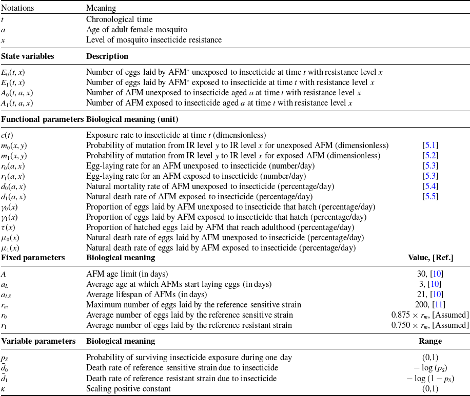


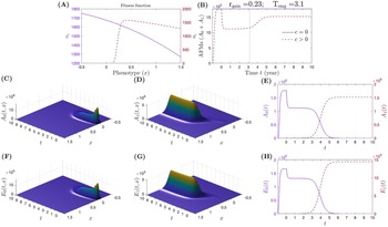


 Open access