


1. Introduction
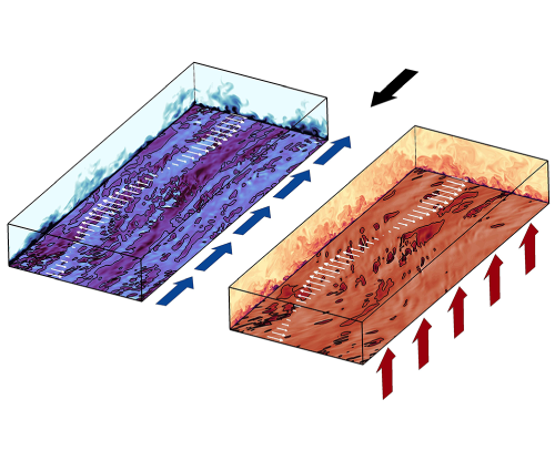
In many industrial applications, controlling heat transfer is as important as controlling drag. Some examples of the kinds of methods to control both drag and heat transfer are given in figure 1. The performance of any given method is commonly based on the changes achieved in the skin-friction coefficient $C_f$
and the Stanton number
$C_f$
and the Stanton number $C_h$
, where
$C_h$
, where
 \begin{equation} C_f \equiv \frac {2\overline {\tau _w}}{\rho U_{{ref}}^2}, \quad C_h \equiv \frac {\overline {q_w}}{\rho c_p U_{{ref}} (T_w - T_{{ref}})}. \end{equation}
Here $\overline {\tau _w}$
,
$\overline {\tau _w}$
, $\overline {q_w}$
,
$\overline {q_w}$
, $\rho$
,
$\rho$
, $c_p$
and
$c_p$
and $T_w$
are the wall shear stress, wall heat flux, fluid density, its specific heat capacity and wall temperature, respectively. The overbar in
$T_w$
are the wall shear stress, wall heat flux, fluid density, its specific heat capacity and wall temperature, respectively. The overbar in $\overline {\tau _w}$
and
$\overline {\tau _w}$
and $\overline {q_w}$
represents averaging over the homogeneous directions and time. In a boundary layer,
$\overline {q_w}$
represents averaging over the homogeneous directions and time. In a boundary layer, $U_{{ref}}$
and
$U_{{ref}}$
and $T_{{ref}}$
are the free-stream velocity and temperature (Walsh & Weinstein Reference Walsh and Weinstein1979), and in a channel flow,
$T_{{ref}}$
are the free-stream velocity and temperature (Walsh & Weinstein Reference Walsh and Weinstein1979), and in a channel flow, $U_{{ref}}$
and
$U_{{ref}}$
and $T_{{ref}}$
are the bulk velocity and either the bulk temperature (Stalio & Nobile Reference Stalio and Nobile2003) or the mixed-mean temperature (Dipprey & Sabersky Reference Dipprey and Sabersky1963; MacDonald et al. Reference MacDonald, Hutchins and Chung2019; Rouhi et al. Reference Rouhi, Endrikat, Modesti, Sandberg, Oda, Tanimoto, Hutchins and Chung2022).
$T_{{ref}}$
are the bulk velocity and either the bulk temperature (Stalio & Nobile Reference Stalio and Nobile2003) or the mixed-mean temperature (Dipprey & Sabersky Reference Dipprey and Sabersky1963; MacDonald et al. Reference MacDonald, Hutchins and Chung2019; Rouhi et al. Reference Rouhi, Endrikat, Modesti, Sandberg, Oda, Tanimoto, Hutchins and Chung2022).
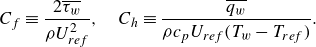
Performance plots showing the fractional changes in the skin-friction coefficient $R_f=C_f/C_{f_0}$
and Stanton number
$R_f=C_f/C_{f_0}$
and Stanton number $R_h=C_h/C_{h_0}$
(log-log scale). The diagonal dashed line represents
$R_h=C_h/C_{h_0}$
(log-log scale). The diagonal dashed line represents $R_h = R_f$
. (a) Grit or irregular roughness (Dipprey & Sabersky Reference Dipprey and Sabersky1963; Forooghi et al. Reference Forooghi, Weidenlener, Magagnato, Böhm, Kubach, Koch and Frohnapfel2018), spherical roughness (Healzer et al. Reference Healzer, Moffat and Kays1974), pin fins (Kang & Kim Reference Kang and Kim1999) and egg-carton roughness (Zhong et al. Reference Zhong, Hutchins and Chung2023; Rowin et al. Reference Rowin, Zhong, Saurav, Jelly, Hutchins and Chung2024). (b) Riblets (Walsh & Weinstein Reference Walsh and Weinstein1979; Choi & Orchard Reference Choi and Orchard1997; Stalio & Nobile Reference Stalio and Nobile2003; Jin & Herwig Reference Jin and Herwig2014; Rouhi et al. Reference Rouhi, Endrikat, Modesti, Sandberg, Oda, Tanimoto, Hutchins and Chung2022; Kuwata Reference Kuwata2022). (c) Wall blowing/suction (Hasegawa & Kasagi Reference Hasegawa and Kasagi2011; Yamamoto et al. Reference Yamamoto, Hasegawa and Kasagi2013). All data points are at
$R_h = R_f$
. (a) Grit or irregular roughness (Dipprey & Sabersky Reference Dipprey and Sabersky1963; Forooghi et al. Reference Forooghi, Weidenlener, Magagnato, Böhm, Kubach, Koch and Frohnapfel2018), spherical roughness (Healzer et al. Reference Healzer, Moffat and Kays1974), pin fins (Kang & Kim Reference Kang and Kim1999) and egg-carton roughness (Zhong et al. Reference Zhong, Hutchins and Chung2023; Rowin et al. Reference Rowin, Zhong, Saurav, Jelly, Hutchins and Chung2024). (b) Riblets (Walsh & Weinstein Reference Walsh and Weinstein1979; Choi & Orchard Reference Choi and Orchard1997; Stalio & Nobile Reference Stalio and Nobile2003; Jin & Herwig Reference Jin and Herwig2014; Rouhi et al. Reference Rouhi, Endrikat, Modesti, Sandberg, Oda, Tanimoto, Hutchins and Chung2022; Kuwata Reference Kuwata2022). (c) Wall blowing/suction (Hasegawa & Kasagi Reference Hasegawa and Kasagi2011; Yamamoto et al. Reference Yamamoto, Hasegawa and Kasagi2013). All data points are at $Pr = 0.7{-}1.0$
.
$Pr = 0.7{-}1.0$
.
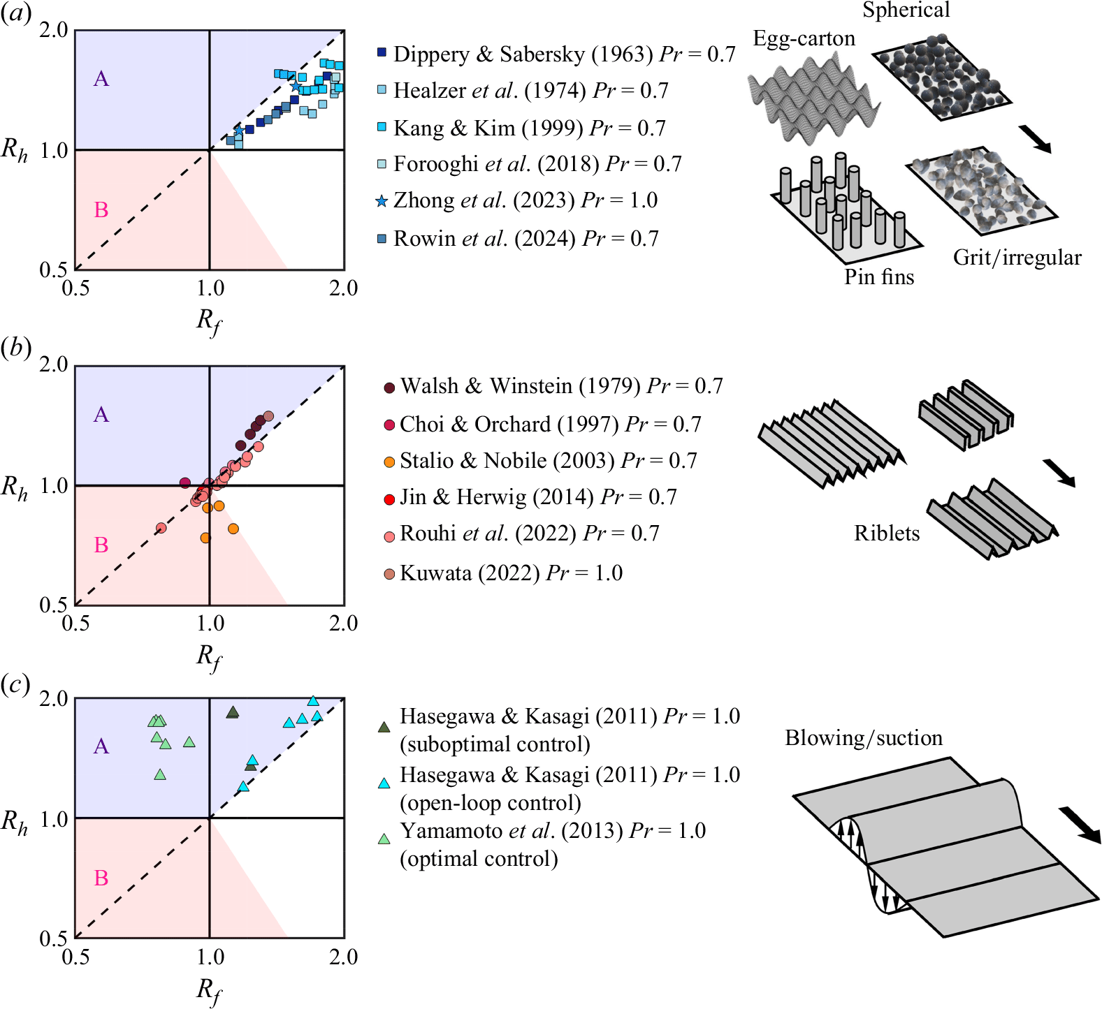
Figure 1 also shows the type of performance plot that is often used to measure the efficacy of control methods (Fan et al. Reference Fan, Ding, Zhang, He and Tao2009; Bunker Reference Bunker2013; Huang et al. Reference Huang, Li, Yu and Tao2017; Rouhi et al. Reference Rouhi, Endrikat, Modesti, Sandberg, Oda, Tanimoto, Hutchins and Chung2022). Here $C_f$
and
$C_f$
and $C_h$
are measured in the flow with control (the target case), and
$C_h$
are measured in the flow with control (the target case), and $C_{f_0}$
and
$C_{f_0}$
and $C_{h_0}$
are measured in the absence of control (the reference case), at matched Reynolds and Prandtl numbers. Some boundary layer studies match Reynolds numbers based on the free-stream velocity and the distance from the inlet (Walsh & Weinstein Reference Walsh and Weinstein1979; Choi & Orchard Reference Choi and Orchard1997). Some channel flow studies match Reynolds numbers based on the channel height and the bulk velocity (Stalio & Nobile Reference Stalio and Nobile2003; Jin & Herwig Reference Jin and Herwig2014; Rouhi et al. Reference Rouhi, Endrikat, Modesti, Sandberg, Oda, Tanimoto, Hutchins and Chung2022) or the friction velocity (MacDonald et al. Reference MacDonald, Hutchins and Chung2019; Zhong et al. Reference Zhong, Hutchins and Chung2023). The diagonal dashed line represents equal fractional change in drag
$C_{h_0}$
are measured in the absence of control (the reference case), at matched Reynolds and Prandtl numbers. Some boundary layer studies match Reynolds numbers based on the free-stream velocity and the distance from the inlet (Walsh & Weinstein Reference Walsh and Weinstein1979; Choi & Orchard Reference Choi and Orchard1997). Some channel flow studies match Reynolds numbers based on the channel height and the bulk velocity (Stalio & Nobile Reference Stalio and Nobile2003; Jin & Herwig Reference Jin and Herwig2014; Rouhi et al. Reference Rouhi, Endrikat, Modesti, Sandberg, Oda, Tanimoto, Hutchins and Chung2022) or the friction velocity (MacDonald et al. Reference MacDonald, Hutchins and Chung2019; Zhong et al. Reference Zhong, Hutchins and Chung2023). The diagonal dashed line represents equal fractional change in drag $R_f$
(
$R_f$
( $=C_f/C_{f_0}$
) and fractional change in heat transfer
$=C_f/C_{f_0}$
) and fractional change in heat transfer $R_h$
(
$R_h$
( $=C_h/C_{h_0}$
). In type A applications (shaded in purple), the objective is to maximise the heat transfer between the fluid and the solid surface, while minimising the drag. Examples include air passages in the gas turbine blades (Baek et al. Reference Baek, Ryu, Bang and Hwang2022; Otto et al. Reference Otto, Kapat, Ricklick and Mhetras2022) or solar air collectors (Vengadesan & Senthil Reference Vengadesan and Senthil2020; Rani & Tripathy Reference Rani and Tripathy2022). In both applications, the air needs to absorb heat from the surface (turbine blade or absorber tube of the collector), yet the friction loss needs to be minimised through the passages. In type B applications (shaded in pink), the objective is to simultaneously minimise the heat transfer and drag between the fluid and the solid surface. Examples include transportation of crude oil (Yu et al. Reference Yu, Li, Zhang, Liu, Zhang, Wei, Sun and Huang2010; Han et al. Reference Han, Yu, Wang, Zhao and Yu2015; Yuan et al. Reference Yuan, Luo, Shi, Gao, Wei, Yu and Chen2023) or transportation of industrial waste heat (Hasegawa et al. Reference Hasegawa, Ishitani, Matsuhashi and Yoshioka1998; Ma et al. Reference Ma, Luo, Wang and Sauce2009; Xie & Jiang Reference Xie and Jiang2017). In these applications, a heated fluid is transported through pipelines to a long-distance demand site, and requires heat loss and friction loss to be minimised.
$=C_h/C_{h_0}$
). In type A applications (shaded in purple), the objective is to maximise the heat transfer between the fluid and the solid surface, while minimising the drag. Examples include air passages in the gas turbine blades (Baek et al. Reference Baek, Ryu, Bang and Hwang2022; Otto et al. Reference Otto, Kapat, Ricklick and Mhetras2022) or solar air collectors (Vengadesan & Senthil Reference Vengadesan and Senthil2020; Rani & Tripathy Reference Rani and Tripathy2022). In both applications, the air needs to absorb heat from the surface (turbine blade or absorber tube of the collector), yet the friction loss needs to be minimised through the passages. In type B applications (shaded in pink), the objective is to simultaneously minimise the heat transfer and drag between the fluid and the solid surface. Examples include transportation of crude oil (Yu et al. Reference Yu, Li, Zhang, Liu, Zhang, Wei, Sun and Huang2010; Han et al. Reference Han, Yu, Wang, Zhao and Yu2015; Yuan et al. Reference Yuan, Luo, Shi, Gao, Wei, Yu and Chen2023) or transportation of industrial waste heat (Hasegawa et al. Reference Hasegawa, Ishitani, Matsuhashi and Yoshioka1998; Ma et al. Reference Ma, Luo, Wang and Sauce2009; Xie & Jiang Reference Xie and Jiang2017). In these applications, a heated fluid is transported through pipelines to a long-distance demand site, and requires heat loss and friction loss to be minimised.
From figure 1(a) we see that rough surfaces and pin fins augment the heat transfer ( $R_h\gt 1$
), but for most data points, the drag increase exceeds the heat transfer increase (
$R_h\gt 1$
), but for most data points, the drag increase exceeds the heat transfer increase ( $R_f\gt R_h \gt 1$
), and so they fall outside the objective space for either type A or B applications. Several phenomena contribute to the imbalance between
$R_f\gt R_h \gt 1$
), and so they fall outside the objective space for either type A or B applications. Several phenomena contribute to the imbalance between $R_f$
and
$R_f$
and $R_h$
. The flow recirculations behind the roughness elements trigger pressure drag in
$R_h$
. The flow recirculations behind the roughness elements trigger pressure drag in $C_f$
, in addition to the viscous drag. However,
$C_f$
, in addition to the viscous drag. However, $C_h$
consists of the wall heat flux only (MacDonald et al. Reference MacDonald, Hutchins and Chung2019), which is the thermal analogue of the viscous stress. Additionally, the recirculation zones break the analogy between the viscous stress and the wall heat flux (MacDonald et al. Reference MacDonald, Hutchins and Chung2019), and the analogy between the turbulent shear stress and the turbulent heat flux (Kuwata Reference Kuwata2021). Also, by increasing the roughness size, the conductive sublayer becomes thinner than the viscous sublayer (MacDonald et al. Reference MacDonald, Hutchins and Chung2019; Zhong et al. Reference Zhong, Hutchins and Chung2023).
$C_h$
consists of the wall heat flux only (MacDonald et al. Reference MacDonald, Hutchins and Chung2019), which is the thermal analogue of the viscous stress. Additionally, the recirculation zones break the analogy between the viscous stress and the wall heat flux (MacDonald et al. Reference MacDonald, Hutchins and Chung2019), and the analogy between the turbulent shear stress and the turbulent heat flux (Kuwata Reference Kuwata2021). Also, by increasing the roughness size, the conductive sublayer becomes thinner than the viscous sublayer (MacDonald et al. Reference MacDonald, Hutchins and Chung2019; Zhong et al. Reference Zhong, Hutchins and Chung2023).
In figure 1(b) we show the performance of riblets, as two-dimensional streamwise-aligned surface protrusions that do not induce pressure drag. Most data points are scattered near $R_h = R_f$
, but a few data points fall into the regions of interest for type A or B applications. Rouhi et al. (Reference Rouhi, Endrikat, Modesti, Sandberg, Oda, Tanimoto, Hutchins and Chung2022) and Kuwata (Reference Kuwata2022) relate such behaviour to the formation of Kelvin–Helmholtz rollers and secondary flows by certain riblet designs.
$R_h = R_f$
, but a few data points fall into the regions of interest for type A or B applications. Rouhi et al. (Reference Rouhi, Endrikat, Modesti, Sandberg, Oda, Tanimoto, Hutchins and Chung2022) and Kuwata (Reference Kuwata2022) relate such behaviour to the formation of Kelvin–Helmholtz rollers and secondary flows by certain riblet designs.
Figure 1(c) shows the data points for wall blowing/suction in a turbulent channel flow. All data points fall into the objective space for type A applications. The data points that noticeably yield $R_h \gt R_f$
are from the application of a suboptimal control framework (Lee et al. Reference Lee, Kim and Choi1998) or an optimal control framework (Bewley et al. Reference Bewley, Moin and Temam2001). Especially, the optimal control application results in simultaneous heat-transfer augmentation and drag reduction (
$R_h \gt R_f$
are from the application of a suboptimal control framework (Lee et al. Reference Lee, Kim and Choi1998) or an optimal control framework (Bewley et al. Reference Bewley, Moin and Temam2001). Especially, the optimal control application results in simultaneous heat-transfer augmentation and drag reduction ( $R_h \gt 1 \gt R_f$
). Hasegawa & Kasagi (Reference Hasegawa and Kasagi2011) and Yamamoto et al. (Reference Yamamoto, Hasegawa and Kasagi2013) discovered that both the optimal and suboptimal control inputs exhibit characteristics similar to a travelling wave. When the coherent part of the suboptimal control inputs are applied as an open-loop control framework, the data points fall closer to
$R_h \gt 1 \gt R_f$
). Hasegawa & Kasagi (Reference Hasegawa and Kasagi2011) and Yamamoto et al. (Reference Yamamoto, Hasegawa and Kasagi2013) discovered that both the optimal and suboptimal control inputs exhibit characteristics similar to a travelling wave. When the coherent part of the suboptimal control inputs are applied as an open-loop control framework, the data points fall closer to $R_h = R_f$
.
$R_h = R_f$
.
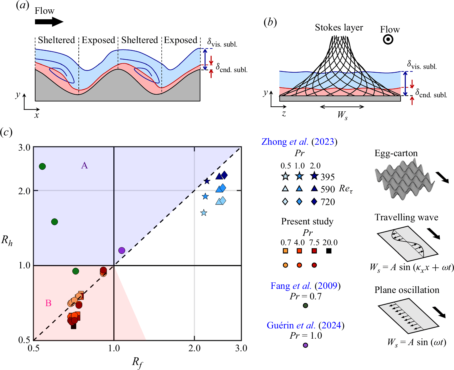
Effect of $Pr$
on the performance of egg-carton roughness by Zhong et al. (Reference Zhong, Hutchins and Chung2023), plane oscillation and a travelling wave from the present study (table 1), and plane oscillation by Fang et al. (Reference Fang, Lu and Shao2009) and Guérin et al. (Reference Guérin, Flageul, Cordier, Grieu and Agostini2024). Star, triangle and diamond symbols represent egg-carton roughness, square symbols represent a streamwise travelling wave (
$Pr$
on the performance of egg-carton roughness by Zhong et al. (Reference Zhong, Hutchins and Chung2023), plane oscillation and a travelling wave from the present study (table 1), and plane oscillation by Fang et al. (Reference Fang, Lu and Shao2009) and Guérin et al. (Reference Guérin, Flageul, Cordier, Grieu and Agostini2024). Star, triangle and diamond symbols represent egg-carton roughness, square symbols represent a streamwise travelling wave ( $\kappa _x \ne 0$
in (1.2)), and circle symbols represent plane oscillation (
$\kappa _x \ne 0$
in (1.2)), and circle symbols represent plane oscillation ( $\kappa _x = 0$
in (1.2)). Panels (a,b) illustrate the different physics underlying the wall heat transfer over roughness and wall oscillation for
$\kappa _x = 0$
in (1.2)). Panels (a,b) illustrate the different physics underlying the wall heat transfer over roughness and wall oscillation for $Pr \gt 1$
;
$Pr \gt 1$
; $\delta _{{vis. \: subl.}}$
and
$\delta _{{vis. \: subl.}}$
and $\delta _{{cnd. \: subl.}}$
respectively indicate the viscous sublayer and conductive sublayer thicknesses. Panel (c) compiles all the data points in the performance plot.
$\delta _{{cnd. \: subl.}}$
respectively indicate the viscous sublayer and conductive sublayer thicknesses. Panel (c) compiles all the data points in the performance plot.
In the present study we focus on wall oscillation either as a spanwise oscillating plane or a streamwise travelling wave, as described by
 \begin{equation} W_s (x,t) = A \sin (\kappa _x x + \omega t), \end{equation}
where $W_s$
is the instantaneous spanwise surface velocity that oscillates with amplitude
$W_s$
is the instantaneous spanwise surface velocity that oscillates with amplitude $A$
and frequency
$A$
and frequency $\omega$
. With
$\omega$
. With $\kappa _x \ne 0$
, the mechanism generates a streamwise travelling wave, and with
$\kappa _x \ne 0$
, the mechanism generates a streamwise travelling wave, and with $\kappa _x = 0$
the motion is a simple spanwise oscillating plane (as illustrated in figure 2). We denote the former case as a travelling wave, and the latter one as plane oscillation. The drag performance of (1.2) has been extensively investigated in the literature (Jung et al. Reference Jung, Mangiavacchi and Akhavan1992; Quadrio & Sibilla Reference Quadrio and Sibilla2000; Quadrio et al. 2009; Viotti et al. Reference Viotti, Quadrio and Luchini2009; Quadrio & Ricco Reference Quadrio and Ricco2011; Quadrio Reference Quadrio2011; Gatti & Quadrio Reference Gatti and Quadrio2013; Hurst et al. Reference Hurst, Yang and Chung2014; Gatti & Quadrio Reference Gatti and Quadrio2016; Marusic et al. Reference Marusic, Chandran, Rouhi, Fu, Wine, Holloway, Chung and Smits2021; Rouhi et al. Reference Rouhi, Fu, Chandran, Zampiron, Smits and Marusic2023; Chandran et al. Reference Chandran, Zampiron, Rouhi, Fu, Wine, Holloway, Smits and Marusic2023).
$\kappa _x = 0$
the motion is a simple spanwise oscillating plane (as illustrated in figure 2). We denote the former case as a travelling wave, and the latter one as plane oscillation. The drag performance of (1.2) has been extensively investigated in the literature (Jung et al. Reference Jung, Mangiavacchi and Akhavan1992; Quadrio & Sibilla Reference Quadrio and Sibilla2000; Quadrio et al. 2009; Viotti et al. Reference Viotti, Quadrio and Luchini2009; Quadrio & Ricco Reference Quadrio and Ricco2011; Quadrio Reference Quadrio2011; Gatti & Quadrio Reference Gatti and Quadrio2013; Hurst et al. Reference Hurst, Yang and Chung2014; Gatti & Quadrio Reference Gatti and Quadrio2016; Marusic et al. Reference Marusic, Chandran, Rouhi, Fu, Wine, Holloway, Chung and Smits2021; Rouhi et al. Reference Rouhi, Fu, Chandran, Zampiron, Smits and Marusic2023; Chandran et al. Reference Chandran, Zampiron, Rouhi, Fu, Wine, Holloway, Smits and Marusic2023).
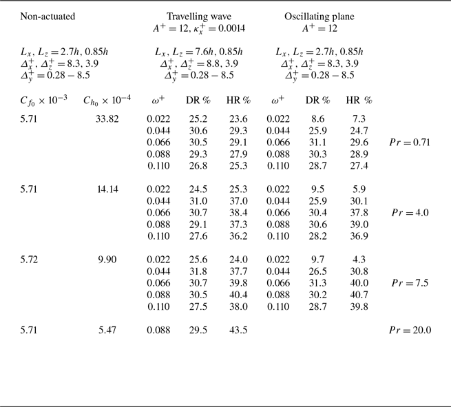
Production calculations at $Re_{\tau _0} = 590$
(reduced domain
$Re_{\tau _0} = 590$
(reduced domain $L_x \ge 2.7h, L_z = 0.85h$
). Non-actuated cases (left column, figure 3
a). Travelling wave cases (middle column, figure 3
b). Spanwise plane oscillation cases (right column, figure 3
c). Each row represents one simulation case. The domain and grid sizes for each configuration are reported at the top.
$L_x \ge 2.7h, L_z = 0.85h$
). Non-actuated cases (left column, figure 3
a). Travelling wave cases (middle column, figure 3
b). Spanwise plane oscillation cases (right column, figure 3
c). Each row represents one simulation case. The domain and grid sizes for each configuration are reported at the top.
Dimensional analysis for the drag yields
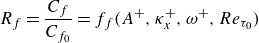 \begin{equation} R_f= \frac{C_f}{C_{f_0}} = f_f (A^+,\kappa ^+_x,\omega ^+,Re_{\tau _0}) \end{equation}
(Marusic et al. Reference Marusic, Chandran, Rouhi, Fu, Wine, Holloway, Chung and Smits2021; Rouhi et al. Reference Rouhi, Fu, Chandran, Zampiron, Smits and Marusic2023). The superscript ‘ $+$
’ indicates normalisation using the viscous velocity (
$+$
’ indicates normalisation using the viscous velocity ( $u_{\tau _0} = \sqrt {\overline {\tau _{w_0}}/\rho }$
) and length (
$u_{\tau _0} = \sqrt {\overline {\tau _{w_0}}/\rho }$
) and length ( $\nu /u_{\tau _0}$
) scales, where
$\nu /u_{\tau _0}$
) scales, where $\nu$
is the fluid kinematic viscosity. The superscript ‘
$\nu$
is the fluid kinematic viscosity. The superscript ‘ $\ast$
’ indicates viscous scaling based on the actual friction velocity, that is,
$\ast$
’ indicates viscous scaling based on the actual friction velocity, that is, $u_{\tau }$
of the drag-altered flow for the actuated cases. For the heat transfer, we need to include the Prandtl number
$u_{\tau }$
of the drag-altered flow for the actuated cases. For the heat transfer, we need to include the Prandtl number $Pr= \nu /\alpha$
, where
$Pr= \nu /\alpha$
, where $\alpha$
is the fluid thermal diffusivity, and we find that
$\alpha$
is the fluid thermal diffusivity, and we find that
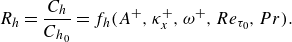 \begin{equation} R_h= \frac{C_h}{C_{h_0}} = f_h (A^+,\kappa ^+_x,\omega ^+,Re_{\tau _0}, Pr). \end{equation}
The drag reduction (DR) is given by ${\textrm{DR}} = 1- R_f$
, and the heat-transfer reduction (HR) is given by
${\textrm{DR}} = 1- R_f$
, and the heat-transfer reduction (HR) is given by ${\textrm{HR}} = 1 - R_h$
. For HR, we have a five-dimensional parameter space (1.4) that is investigated over a limited extent (Fang et al. Reference Fang, Lu and Shao2009, Reference Fang, Lu and Shao2010; Guérin et al. Reference Guérin, Flageul, Cordier, Grieu and Agostini2024), as shown in figure 2. These studies consider spanwise plane oscillation
${\textrm{HR}} = 1 - R_h$
. For HR, we have a five-dimensional parameter space (1.4) that is investigated over a limited extent (Fang et al. Reference Fang, Lu and Shao2009, Reference Fang, Lu and Shao2010; Guérin et al. Reference Guérin, Flageul, Cordier, Grieu and Agostini2024), as shown in figure 2. These studies consider spanwise plane oscillation $(\kappa ^+_x = 0)$
in a turbulent channel flow at
$(\kappa ^+_x = 0)$
in a turbulent channel flow at $Re_{\tau _0} = h u_{\tau _0}/\nu \simeq 180$
and
$Re_{\tau _0} = h u_{\tau _0}/\nu \simeq 180$
and $Pr \simeq 0.7 - 1.0$
. Fang et al. (Reference Fang, Lu and Shao2009, Reference Fang, Lu and Shao2010) consider three cases with
$Pr \simeq 0.7 - 1.0$
. Fang et al. (Reference Fang, Lu and Shao2009, Reference Fang, Lu and Shao2010) consider three cases with $T^+_{osc} = 2\pi /\omega ^+ = 100$
and
$T^+_{osc} = 2\pi /\omega ^+ = 100$
and $A^+ = 6, 13, 19$
, and Guérin et al. (Reference Guérin, Flageul, Cordier, Grieu and Agostini2024) consider one case with
$A^+ = 6, 13, 19$
, and Guérin et al. (Reference Guérin, Flageul, Cordier, Grieu and Agostini2024) consider one case with $T^+_{osc} = 500$
and
$T^+_{osc} = 500$
and $A^+ = 30$
. These cases fall into the objective space for type A applications (except one case with
$A^+ = 30$
. These cases fall into the objective space for type A applications (except one case with $R_f \lt 1, R_h \simeq 1$
).
$R_f \lt 1, R_h \simeq 1$
).
Figure 2 highlights that we are at an early stage in terms of our knowledge of HR for the surface actuation (1.2), and just like the investigations on DR, we need to explore different parameters of (1.4) as a build up process. Comparing (1.4) with (1.3), $Pr$
is a key parameter that differentiates
$Pr$
is a key parameter that differentiates $R_h$
from
$R_h$
from $R_f$
, and it leads to their significant disparity (figure 2). Furthermore, the fluids for type B applications have
$R_f$
, and it leads to their significant disparity (figure 2). Furthermore, the fluids for type B applications have $Pr \gg 1$
(e.g. crude oil). Therefore, in the present study we focus on
$Pr \gg 1$
(e.g. crude oil). Therefore, in the present study we focus on $Pr$
and
$Pr$
and $\omega ^+$
as our parameters of interest (figure 2 and table 1). We conduct direct numerical simulations (DNS) of turbulent forced convection in a half-channel flow with fix
$\omega ^+$
as our parameters of interest (figure 2 and table 1). We conduct direct numerical simulations (DNS) of turbulent forced convection in a half-channel flow with fix $A^+ = 12$
and
$A^+ = 12$
and $Re_{\tau _0} = 590$
, and we consider two values for
$Re_{\tau _0} = 590$
, and we consider two values for $\kappa ^+_x$
to simulate plane oscillation (
$\kappa ^+_x$
to simulate plane oscillation ( $\kappa ^+_x = 0$
) and a travelling wave (
$\kappa ^+_x = 0$
) and a travelling wave ( $\kappa ^+_x = 0.0014$
,
$\kappa ^+_x = 0.0014$
, $\lambda ^+ = 2\pi /\kappa ^+_x \simeq 4500$
). We consider
$\lambda ^+ = 2\pi /\kappa ^+_x \simeq 4500$
). We consider $Pr = 0.71$
(air),
$Pr = 0.71$
(air), $4.0$
,
$4.0$
, $7.5$
(water) and
$7.5$
(water) and $20$
(molten salt). At each
$20$
(molten salt). At each $0.71 \le Pr \le 7.5$
, we systematically vary
$0.71 \le Pr \le 7.5$
, we systematically vary $\omega ^+$
from
$\omega ^+$
from $0.022$
to
$0.022$
to $0.110$
, corresponding to the regime where we expect DR to reach
$0.110$
, corresponding to the regime where we expect DR to reach $30\,\%$
(Gatti & Quadrio Reference Gatti and Quadrio2016; Rouhi et al. Reference Rouhi, Fu, Chandran, Zampiron, Smits and Marusic2023). Our preference for the present actuation parameters is motivated by an existing surface-actuation test bed (Marusic et al. Reference Marusic, Chandran, Rouhi, Fu, Wine, Holloway, Chung and Smits2021; Chandran et al. Reference Chandran, Zampiron, Rouhi, Fu, Wine, Holloway, Smits and Marusic2023) that can operate under these conditions. This provides the opportunity to extend the present numerical study through experiment. As the first study that investigates
$30\,\%$
(Gatti & Quadrio Reference Gatti and Quadrio2016; Rouhi et al. Reference Rouhi, Fu, Chandran, Zampiron, Smits and Marusic2023). Our preference for the present actuation parameters is motivated by an existing surface-actuation test bed (Marusic et al. Reference Marusic, Chandran, Rouhi, Fu, Wine, Holloway, Chung and Smits2021; Chandran et al. Reference Chandran, Zampiron, Rouhi, Fu, Wine, Holloway, Smits and Marusic2023) that can operate under these conditions. This provides the opportunity to extend the present numerical study through experiment. As the first study that investigates $Pr$
effects for this problem, we conduct a thorough study of grid resolution requirements for our considered parameter space (Appendix A).
$Pr$
effects for this problem, we conduct a thorough study of grid resolution requirements for our considered parameter space (Appendix A).
As an overview, we note that all our results give a decrease in drag and heat transfer, with maximum ${\textrm{DR}}=30\,\%$
and
${\textrm{DR}}=30\,\%$
and ${\textrm{HR}}=40\,\%$
(see figure 2). For Prandtl numbers greater than one, however, HR increases more than DR. The results fall into the objective space for type B applications, a space that has largely been neglected in the past despite its industrial relevance. The surfaces that we reviewed in figure 1 consider
${\textrm{HR}}=40\,\%$
(see figure 2). For Prandtl numbers greater than one, however, HR increases more than DR. The results fall into the objective space for type B applications, a space that has largely been neglected in the past despite its industrial relevance. The surfaces that we reviewed in figure 1 consider $Pr = 0.7 - 1.0$
, however, we anticipate that their performances will change with increasing
$Pr = 0.7 - 1.0$
, however, we anticipate that their performances will change with increasing $Pr$
. For instance, in figure 2 we overlay the data points of egg-carton roughness at
$Pr$
. For instance, in figure 2 we overlay the data points of egg-carton roughness at $Pr = 0.5, 1.0, 2.0$
by Zhong et al. (Reference Zhong, Hutchins and Chung2023). Unlike plane oscillation or a travelling wave, the roughness data points approach
$Pr = 0.5, 1.0, 2.0$
by Zhong et al. (Reference Zhong, Hutchins and Chung2023). Unlike plane oscillation or a travelling wave, the roughness data points approach $R_h = R_f$
with increasing
$R_h = R_f$
with increasing $Pr$
because heat transfer over these two surface types is governed by different flow mechanisms that are unique to each surface, leading to different trends with
$Pr$
because heat transfer over these two surface types is governed by different flow mechanisms that are unique to each surface, leading to different trends with $Pr$
. Over the rough surface (figure 2
a), variation of
$Pr$
. Over the rough surface (figure 2
a), variation of $C_h$
with
$C_h$
with $Pr$
depends on the area fraction of the sheltered and exposed regions, associated with the recirculation and attached zones that follow different local
$Pr$
depends on the area fraction of the sheltered and exposed regions, associated with the recirculation and attached zones that follow different local $Pr$
scalings (Zhong et al. Reference Zhong, Hutchins and Chung2023; Rowin et al. Reference Rowin, Zhong, Saurav, Jelly, Hutchins and Chung2024). Over the surface oscillation (figure 2
b), the variation of
$Pr$
scalings (Zhong et al. Reference Zhong, Hutchins and Chung2023; Rowin et al. Reference Rowin, Zhong, Saurav, Jelly, Hutchins and Chung2024). Over the surface oscillation (figure 2
b), the variation of $C_h$
with
$C_h$
with $Pr$
is an aspect that we investigate in the present study. We discover that by increasing
$Pr$
is an aspect that we investigate in the present study. We discover that by increasing $Pr$
and thinning of the conductive sublayer, the Stokes layer, formed in response to the wall oscillation, transfers more energy to the near-wall temperature scales than the velocity scales. We also find that HR yields different
$Pr$
and thinning of the conductive sublayer, the Stokes layer, formed in response to the wall oscillation, transfers more energy to the near-wall temperature scales than the velocity scales. We also find that HR yields different $Pr$
scaling depending on the actuation parameters. In § 3.5 we derive a model that predicts that plane oscillation and a travelling wave can reduce the heat loss beyond
$Pr$
scaling depending on the actuation parameters. In § 3.5 we derive a model that predicts that plane oscillation and a travelling wave can reduce the heat loss beyond $50\,\%$
for
$50\,\%$
for $Pr \gtrsim \mathcal{O}(10^2)$
, a regime that is important for crude oil transportation through pipelines. Our model is supported by our DNS data point at
$Pr \gtrsim \mathcal{O}(10^2)$
, a regime that is important for crude oil transportation through pipelines. Our model is supported by our DNS data point at $Pr = 20$
that yields
$Pr = 20$
that yields ${\textrm{HR}} = 43\,\%$
(black square in figure 2).
${\textrm{HR}} = 43\,\%$
(black square in figure 2).
2. Numerical flow set-up
2.1. Governing equations and simulation set-up
The governing equations for an incompressible fluid with constant $\rho, \nu$
and thermal diffusivity
$\rho, \nu$
and thermal diffusivity $\alpha$
are solved in a half-channel flow (figure 3), where
$\alpha$
are solved in a half-channel flow (figure 3), where
 \begin{align} &\boldsymbol {\nabla }\boldsymbol {\cdot }\mathbf{U} = 0, \end{align}
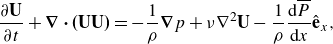 \begin{align} \frac {\partial \mathbf{U}}{\partial t} + \boldsymbol {\nabla }\boldsymbol {\cdot }\mathbf{(UU)} &= -\frac {1}{\rho }\boldsymbol {\nabla }p + \nu \nabla ^2 \mathbf{U} -\frac {1}{\rho }\frac {\textrm{d}\overline {P}}{\textrm{d}x}\hat {\mathbf{e}}_x, \end{align}
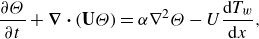 \begin{align} \frac {\partial \Theta }{\partial t} + \boldsymbol {\nabla }\boldsymbol {\cdot }(&\mathbf{U}\Theta ) = \alpha \nabla ^2 \Theta -U\frac {\textrm{d}T_w}{\textrm{d}x}, \end{align}
and (2.1), (2.2) and (2.3) are the continuity, velocity and temperature transport equations, respectively. We ignore buoyancy, as appropriate for forced convection. In our notation, $\mathbf{U} = (U,V,W)$
is the velocity vector, and
$\mathbf{U} = (U,V,W)$
is the velocity vector, and $x$
,
$x$
, $y$
and
$y$
and $z$
are the streamwise, wall-normal and spanwise directions, respectively. In (2.2) the total pressure gradient was decomposed into the driving (mean) part
$z$
are the streamwise, wall-normal and spanwise directions, respectively. In (2.2) the total pressure gradient was decomposed into the driving (mean) part $\textrm{d}\overline {P}/\textrm{d}x$
and the periodic part
$\textrm{d}\overline {P}/\textrm{d}x$
and the periodic part $\boldsymbol {\nabla } p$
. Similarly, the total temperature
$\boldsymbol {\nabla } p$
. Similarly, the total temperature $T = (\textrm{dT}_w/\textrm{dx})x + \Theta$
was decomposed into the mean part
$T = (\textrm{dT}_w/\textrm{dx})x + \Theta$
was decomposed into the mean part $\textrm{dT}_w/\textrm{dx}$
and the periodic part
$\textrm{dT}_w/\textrm{dx}$
and the periodic part $\Theta$
. This thermal driving approach imposes a prescribed mean heat flux at the wall, making it a suitable boundary condition for a periodic domain, and it has been widely used for the simulation of forced convection in a channel flow (Kasagi et al. Reference Kasagi, Tomita and Kuroda1992; Watanabe & Takahashi Reference Watanabe and Takahashi2002; Stalio & Nobile Reference Stalio and Nobile2003; Jin & Herwig Reference Jin and Herwig2014; Alcántara-Á vila & Hoyas Reference Alcántara-Á vila and Hoyas2021; Alcántara-Á vila et al. Reference Alcántara-Á vila and Pérez-Quiles2021; Rouhi et al. Reference Rouhi, Endrikat, Modesti, Sandberg, Oda, Tanimoto, Hutchins and Chung2022). By averaging (2.2) and (2.3) in time and over the entire fluid domain, we obtain
$\Theta$
. This thermal driving approach imposes a prescribed mean heat flux at the wall, making it a suitable boundary condition for a periodic domain, and it has been widely used for the simulation of forced convection in a channel flow (Kasagi et al. Reference Kasagi, Tomita and Kuroda1992; Watanabe & Takahashi Reference Watanabe and Takahashi2002; Stalio & Nobile Reference Stalio and Nobile2003; Jin & Herwig Reference Jin and Herwig2014; Alcántara-Á vila & Hoyas Reference Alcántara-Á vila and Hoyas2021; Alcántara-Á vila et al. Reference Alcántara-Á vila and Pérez-Quiles2021; Rouhi et al. Reference Rouhi, Endrikat, Modesti, Sandberg, Oda, Tanimoto, Hutchins and Chung2022). By averaging (2.2) and (2.3) in time and over the entire fluid domain, we obtain
 \begin{equation} -\frac {1}{\rho }\frac {\textrm{d}\overline {P}}{\textrm{d}x}h = \frac {\overline {\tau _w}}{\rho } \equiv u^2_\tau, \qquad -U_b \frac {\textrm{d}T_w}{\textrm{d}x}h = \frac {\overline {q_w}}{\rho c_p} \equiv \theta _\tau u_\tau, \end{equation}
where $\overline {\tau _w}$
and
$\overline {\tau _w}$
and $\overline { q_w }$
are respectively the
$\overline { q_w }$
are respectively the $xz$
plane and time-averaged wall shear stress and wall heat flux,
$xz$
plane and time-averaged wall shear stress and wall heat flux, $U_b$
is the bulk velocity,
$U_b$
is the bulk velocity, $h$
is the half-channel height,
$h$
is the half-channel height, $u_\tau$
and
$u_\tau$
and $\theta _\tau$
are the friction velocity and friction temperature, and
$\theta _\tau$
are the friction velocity and friction temperature, and $c_p$
is the specific heat capacity. We adjust
$c_p$
is the specific heat capacity. We adjust $\textrm{d}\overline {P}/\textrm{dx}$
based on a target flow rate (namely, a bulk Reynolds number
$\textrm{d}\overline {P}/\textrm{dx}$
based on a target flow rate (namely, a bulk Reynolds number $Re_b \equiv U_b h / \nu$
) that is matched between the non-actuated reference case (figure 3
a) and the actuated cases (figure 3
b,c).
$Re_b \equiv U_b h / \nu$
) that is matched between the non-actuated reference case (figure 3
a) and the actuated cases (figure 3
b,c).
Computational configurations in a half-channel flow for the present study. (a) Non-actuated case as the reference. (b) Actuated case with the travelling wave with $A^+ = 12$
,
$A^+ = 12$
, $\kappa ^+_x = 0.0014$
; the domain length encompasses one wavelength
$\kappa ^+_x = 0.0014$
; the domain length encompasses one wavelength $L_x = 2\pi /\kappa _x \simeq 7.6h$
. (c) Actuated case with spanwise plane oscillation with
$L_x = 2\pi /\kappa _x \simeq 7.6h$
. (c) Actuated case with spanwise plane oscillation with $A^+ = 12$
. In (b,c) we overlay the instantaneous wall motion as a vector field. Full domain shown by the large box with black edges; reduced domain shown by the small box with white edges. In (a,b,c) we visualise the instantaneous fields of
$A^+ = 12$
. In (b,c) we overlay the instantaneous wall motion as a vector field. Full domain shown by the large box with black edges; reduced domain shown by the small box with white edges. In (a,b,c) we visualise the instantaneous fields of $\Theta$
at
$\Theta$
at $y^+ = 15, Re_{\tau _0} = 590$
and
$y^+ = 15, Re_{\tau _0} = 590$
and $Pr = 7.5$
, and for
$Pr = 7.5$
, and for $\omega ^+ = 0.088$
in (b,c).
$\omega ^+ = 0.088$
in (b,c).

Equations (2.1)--(2.3) are solved using a fully conservative fourth-order finite difference code, employed by previous DNS studies of thermal convection (Ng et al. Reference Ng, Ooi, Lohse and Chung2015; Rouhi et al. Reference Rouhi, Lohse, Marusic, Sun and Chung2021; Zhong et al. Reference Zhong, Hutchins and Chung2023; Rowin et al. Reference Rowin, Zhong, Saurav, Jelly, Hutchins and Chung2024). The half-channel flow has periodic boundary conditions in the streamwise and spanwise directions (figure 3). The bottom-wall velocity boundary conditions are $U=V=W = 0$
for the non-actuated case (figure 3
a),
$U=V=W = 0$
for the non-actuated case (figure 3
a), $U=V=0$
,
$U=V=0$
, $W = A \sin (\kappa _x x + \omega t)$
for the actuated case with the travelling wave (figure 3
b) and
$W = A \sin (\kappa _x x + \omega t)$
for the actuated case with the travelling wave (figure 3
b) and $U=V=0$
,
$U=V=0$
, $W = A \sin (\omega t)$
for the actuated case with the spanwise plane oscillation (figure 3
c). The top boundary conditions for the velocity are the free-slip and impermeable conditions
$W = A \sin (\omega t)$
for the actuated case with the spanwise plane oscillation (figure 3
c). The top boundary conditions for the velocity are the free-slip and impermeable conditions $(\partial U/\partial y = \partial W/\partial y = V = 0)$
. The boundary conditions for
$(\partial U/\partial y = \partial W/\partial y = V = 0)$
. The boundary conditions for $\Theta$
at the bottom wall and top boundary are
$\Theta$
at the bottom wall and top boundary are $\Theta = 0$
and
$\Theta = 0$
and $\partial \Theta / \partial y = 0$
, respectively. In other words, the total temperature at the bottom wall increases linearly in the
$\partial \Theta / \partial y = 0$
, respectively. In other words, the total temperature at the bottom wall increases linearly in the $x$
direction
$x$
direction $T = (\textrm{dT}_w/\textrm{dx})x$
, and at the top boundary the boundary condition is adiabatic (
$T = (\textrm{dT}_w/\textrm{dx})x$
, and at the top boundary the boundary condition is adiabatic ( $\partial T / \partial y = 0$
). Past studies have employed half-channel flow to study turbulent flow over complex surfaces (Yuan & Piomelli Reference Yuan and Piomelli2014; MacDonald et al. Reference MacDonald, Chung, Hutchins, Chan, Ooi and García-Mayoral2017; Rouhi et al. 2019). This configuration has a lower computational cost compared with the conventional Poiseuille channel flow with a no-slip condition at the bottom and top walls. Yet the two configurations have almost identical mean velocity profiles up to the logarithmic region, and similar turbulent stresses (Yao et al. Reference Yao, Chen and Hussain2022). This is also supported in Appendix A, where we obtain very similar mean velocity and turbulent stress profiles between our non-actuated half-channel flow and the DNS of a Poiseuille channel flow by Moser et al. (Reference Moser, Kim and Mansour1999) (figure 25
a,b), and the values of
$\partial T / \partial y = 0$
). Past studies have employed half-channel flow to study turbulent flow over complex surfaces (Yuan & Piomelli Reference Yuan and Piomelli2014; MacDonald et al. Reference MacDonald, Chung, Hutchins, Chan, Ooi and García-Mayoral2017; Rouhi et al. 2019). This configuration has a lower computational cost compared with the conventional Poiseuille channel flow with a no-slip condition at the bottom and top walls. Yet the two configurations have almost identical mean velocity profiles up to the logarithmic region, and similar turbulent stresses (Yao et al. Reference Yao, Chen and Hussain2022). This is also supported in Appendix A, where we obtain very similar mean velocity and turbulent stress profiles between our non-actuated half-channel flow and the DNS of a Poiseuille channel flow by Moser et al. (Reference Moser, Kim and Mansour1999) (figure 25
a,b), and the values of $C_{f_0}$
differ by less than
$C_{f_0}$
differ by less than $2\,\%$
.
$2\,\%$
.
Throughout this paper, we call $\Theta$
the temperature. We denote the
$\Theta$
the temperature. We denote the $xz$
plane and time-averaged quantities with overbars (e.g.
$xz$
plane and time-averaged quantities with overbars (e.g. $\overline {\Theta }$
is the plane and time averaged
$\overline {\Theta }$
is the plane and time averaged $\Theta$
) and the turbulent quantities with lowercase letters (e.g.
$\Theta$
) and the turbulent quantities with lowercase letters (e.g. $\theta$
is the turbulent temperature). Following this notation,
$\theta$
is the turbulent temperature). Following this notation, $\overline {u^2}$
and
$\overline {u^2}$
and $ \overline {uv}$
are the turbulent stress components, and
$ \overline {uv}$
are the turbulent stress components, and $\overline {\theta ^2}$
and
$\overline {\theta ^2}$
and $ \overline {\theta v}$
are their analogue for the turbulent temperature fluxes.
$ \overline {\theta v}$
are their analogue for the turbulent temperature fluxes.
2.2. Simulation cases
Table 1 summarises the production calculations. All the calculations were performed at a fixed bulk Reynolds number $Re_b \simeq 11004$
, equivalent to a friction Reynolds number
$Re_b \simeq 11004$
, equivalent to a friction Reynolds number $Re_{\tau _0} = 590$
for the non-actuated flow. The grid sizes are
$Re_{\tau _0} = 590$
for the non-actuated flow. The grid sizes are $\unicode{x1D6E5} ^+_x \times \unicode{x1D6E5} ^+_z \simeq 8 \times 4, \unicode{x1D6E5} ^+_y = 0.28 - 8.5$
, chosen based on extensive validation studies (Appendix A). In comparison, Alcántara-Á vila & Hoyas (Reference Alcántara-Á vila and Hoyas2021) used
$\unicode{x1D6E5} ^+_x \times \unicode{x1D6E5} ^+_z \simeq 8 \times 4, \unicode{x1D6E5} ^+_y = 0.28 - 8.5$
, chosen based on extensive validation studies (Appendix A). In comparison, Alcántara-Á vila & Hoyas (Reference Alcántara-Á vila and Hoyas2021) used $\unicode{x1D6E5} ^+_x \times \unicode{x1D6E5} ^+_z \simeq 8 \times 4, \unicode{x1D6E5} ^+_y = 0.27 - 5.3$
for the turbulent channel flow at
$\unicode{x1D6E5} ^+_x \times \unicode{x1D6E5} ^+_z \simeq 8 \times 4, \unicode{x1D6E5} ^+_y = 0.27 - 5.3$
for the turbulent channel flow at $Re_{\tau _0} = 500$
and
$Re_{\tau _0} = 500$
and $1 \le Pr \le 7$
, and Pirozzoli (Reference Pirozzoli2023) used
$1 \le Pr \le 7$
, and Pirozzoli (Reference Pirozzoli2023) used $\unicode{x1D6E5} ^+_x \times \unicode{x1D6E5} ^+_z \simeq 10 \times 4.5$
with
$\unicode{x1D6E5} ^+_x \times \unicode{x1D6E5} ^+_z \simeq 10 \times 4.5$
with $30$
points within
$30$
points within $y^+ \le 40$
for the turbulent pipe flow at
$y^+ \le 40$
for the turbulent pipe flow at $Re_{\tau _0} \simeq 1100$
and
$Re_{\tau _0} \simeq 1100$
and $Pr \le 16$
. Here, we have
$Pr \le 16$
. Here, we have $60$
points within
$60$
points within $y^+ \le 40$
. As shown in Appendix A, we obtain less than
$y^+ \le 40$
. As shown in Appendix A, we obtain less than $2\,\%$
difference in DR and HR when using finer resolutions than our production calculation grids, and find very good agreement in the first- and second-order velocity and temperature statistics as well as their spectrograms (figures 25 to 27).
$2\,\%$
difference in DR and HR when using finer resolutions than our production calculation grids, and find very good agreement in the first- and second-order velocity and temperature statistics as well as their spectrograms (figures 25 to 27).
To reduce the computational cost, the production calculations were performed in a reduced domain rather than a full-domain conventional channel flow (see figure 3). Because of the domain truncation, the flow is fully resolved up to a fraction of the domain height $y_{{res}} \lt h$
(figure 4). In the past, the reduced-domain channel flow has been used for accurate calculation of the drag and the near-wall turbulence over various static and deforming surfaces, including egg-carton roughness with
$y_{{res}} \lt h$
(figure 4). In the past, the reduced-domain channel flow has been used for accurate calculation of the drag and the near-wall turbulence over various static and deforming surfaces, including egg-carton roughness with $y^+_{{res}} \lesssim 250$
(MacDonald et al. Reference MacDonald, Chung, Hutchins, Chan, Ooi and García-Mayoral2017, Reference MacDonald, Ooi, García-Mayoral, Hutchins and Chung2018), riblets with
$y^+_{{res}} \lesssim 250$
(MacDonald et al. Reference MacDonald, Chung, Hutchins, Chan, Ooi and García-Mayoral2017, Reference MacDonald, Ooi, García-Mayoral, Hutchins and Chung2018), riblets with $y^+_{{res}} \simeq 100$
(Endrikat et al. Reference Endrikat, Modesti, MacDonald, García-Mayoral, Hutchins and Chung2021) and travelling waves with
$y^+_{{res}} \simeq 100$
(Endrikat et al. Reference Endrikat, Modesti, MacDonald, García-Mayoral, Hutchins and Chung2021) and travelling waves with $y^+_{{res}} \lesssim 1000$
(Gatti & Quadrio Reference Gatti and Quadrio2016; Rouhi et al. Reference Rouhi, Fu, Chandran, Zampiron, Smits and Marusic2023). The reduced-domain channel flow has also been employed for accurate calculation of the wall heat flux and the near-wall thermal field over rough surfaces with
$y^+_{{res}} \lesssim 1000$
(Gatti & Quadrio Reference Gatti and Quadrio2016; Rouhi et al. Reference Rouhi, Fu, Chandran, Zampiron, Smits and Marusic2023). The reduced-domain channel flow has also been employed for accurate calculation of the wall heat flux and the near-wall thermal field over rough surfaces with $y^+_{{res}} \lesssim 600$
(MacDonald et al. Reference MacDonald, Hutchins and Chung2019; Zhong et al. Reference Zhong, Hutchins and Chung2023; Rowin et al. Reference Rowin, Zhong, Saurav, Jelly, Hutchins and Chung2024), and riblets with
$y^+_{{res}} \lesssim 600$
(MacDonald et al. Reference MacDonald, Hutchins and Chung2019; Zhong et al. Reference Zhong, Hutchins and Chung2023; Rowin et al. Reference Rowin, Zhong, Saurav, Jelly, Hutchins and Chung2024), and riblets with $y^+_{{res}} \simeq 100$
(Rouhi et al. Reference Rouhi, Endrikat, Modesti, Sandberg, Oda, Tanimoto, Hutchins and Chung2022). In our case, as shown in Appendix A, with
$y^+_{{res}} \simeq 100$
(Rouhi et al. Reference Rouhi, Endrikat, Modesti, Sandberg, Oda, Tanimoto, Hutchins and Chung2022). In our case, as shown in Appendix A, with $\unicode{x1D6E5} ^+_x \times \unicode{x1D6E5} ^+_z \simeq 8 \times 4$
the difference between the reduced and full domains is less than
$\unicode{x1D6E5} ^+_x \times \unicode{x1D6E5} ^+_z \simeq 8 \times 4$
the difference between the reduced and full domains is less than $1\,\%$
in terms of DR and HR. Furthermore, the results for the two domain sizes agree well in terms of the statistics of velocity and temperature, and their spectrograms (figures 26 and 27). For the reduced-domain sizes, we follow the prescriptions by Chung et al. (Reference Chung, Chan, MacDonald, Hutchins and Ooi2015) and MacDonald et al. (Reference MacDonald, Chung, Hutchins, Chan, Ooi and García-Mayoral2017), which were extended to the travelling wave actuation case by Rouhi et al. (Reference Rouhi, Fu, Chandran, Zampiron, Smits and Marusic2023). The resolved height
$1\,\%$
in terms of DR and HR. Furthermore, the results for the two domain sizes agree well in terms of the statistics of velocity and temperature, and their spectrograms (figures 26 and 27). For the reduced-domain sizes, we follow the prescriptions by Chung et al. (Reference Chung, Chan, MacDonald, Hutchins and Ooi2015) and MacDonald et al. (Reference MacDonald, Chung, Hutchins, Chan, Ooi and García-Mayoral2017), which were extended to the travelling wave actuation case by Rouhi et al. (Reference Rouhi, Fu, Chandran, Zampiron, Smits and Marusic2023). The resolved height $y^+_{{res}}$
needs to fall in the logarithmic region, and the domain width
$y^+_{{res}}$
needs to fall in the logarithmic region, and the domain width $L^+_z$
and length
$L^+_z$
and length $L^+_x$
are adjusted so that
$L^+_x$
are adjusted so that $L^+_z \simeq 2.5 y^+_{{res}}$
and
$L^+_z \simeq 2.5 y^+_{{res}}$
and $ L^+_x \gtrsim \max {(3L^+_z,1000,\lambda ^+)}$
, where
$ L^+_x \gtrsim \max {(3L^+_z,1000,\lambda ^+)}$
, where $\lambda = 2\pi /\kappa _x$
is the travelling wavelength. Here, we chose
$\lambda = 2\pi /\kappa _x$
is the travelling wavelength. Here, we chose $y^+_{{res}} = 200$
, which resolves up to a third of the half-channel height. Hence, the domain sizes are
$y^+_{{res}} = 200$
, which resolves up to a third of the half-channel height. Hence, the domain sizes are $L_x \times L_z \simeq 2.7 h \times 0.85 h$
for the non-actuated and plane oscillation cases (figure 3
a,c). For the travelling wave cases, however,
$L_x \times L_z \simeq 2.7 h \times 0.85 h$
for the non-actuated and plane oscillation cases (figure 3
a,c). For the travelling wave cases, however, $L_x$
cannot be truncated because it is constrained by the travelling wavelength
$L_x$
cannot be truncated because it is constrained by the travelling wavelength $\lambda \simeq 7.6 h$
, and so we use
$\lambda \simeq 7.6 h$
, and so we use $L_x \times L_z \simeq 7.6 h \times 0.85 h$
(figure 3
b). For the actuated cases,
$L_x \times L_z \simeq 7.6 h \times 0.85 h$
(figure 3
b). For the actuated cases, $y_{{res}}$
scaled by the actuated (drag-reduced) friction velocity is
$y_{{res}}$
scaled by the actuated (drag-reduced) friction velocity is $170 \lesssim y^*_{{res}} \lesssim 190$
(that is, less than 200). Therefore,
$170 \lesssim y^*_{{res}} \lesssim 190$
(that is, less than 200). Therefore, $y^*_{{res}} = 170$
is taken to be the maximum resolved height for all our cases.
$y^*_{{res}} = 170$
is taken to be the maximum resolved height for all our cases.
Comparison at $Re_{\tau _0} = 590$
of (a) mean velocity
$Re_{\tau _0} = 590$
of (a) mean velocity $\overline {U}^*$
and (b) mean temperature
$\overline {U}^*$
and (b) mean temperature $\overline {\Theta }^*$
between the full-domain (grey lines) and reduced-domain half-channel flow (black, blue and red lines). Black lines: non-actuated case at
$\overline {\Theta }^*$
between the full-domain (grey lines) and reduced-domain half-channel flow (black, blue and red lines). Black lines: non-actuated case at $Pr = 7.5$
. Blue and red lines: travelling wave case at
$Pr = 7.5$
. Blue and red lines: travelling wave case at $Pr=7.5$
with
$Pr=7.5$
with $A^+ = 12$
,
$A^+ = 12$
, $\kappa ^+_x = 0.0014$
,
$\kappa ^+_x = 0.0014$
, $\omega ^+ = 0.088$
. For the reduced-domain cases, the resolved portion is shown with a dashed line (
$\omega ^+ = 0.088$
. For the reduced-domain cases, the resolved portion is shown with a dashed line ( $y^* \lesssim 170$
) and the unresolved portion is shown with a dashed-dotted line (
$y^* \lesssim 170$
) and the unresolved portion is shown with a dashed-dotted line ( $y^* \gtrsim 170$
). The unresolved portion is replaced by the reconstructed profiles (solid lines), as explained in § 2.3. The insets plot the velocity and temperature differences
$y^* \gtrsim 170$
). The unresolved portion is replaced by the reconstructed profiles (solid lines), as explained in § 2.3. The insets plot the velocity and temperature differences $\unicode{x1D6E5} \overline {U}^*$
and
$\unicode{x1D6E5} \overline {U}^*$
and $\unicode{x1D6E5} \overline {\Theta }^*$
; bullets mark
$\unicode{x1D6E5} \overline {\Theta }^*$
; bullets mark $y^*_{{res}} = 170$
, where we obtain the log-law shifts
$y^*_{{res}} = 170$
, where we obtain the log-law shifts $\unicode{x1D6E5} \overline {U}^*_{{log}}$
and
$\unicode{x1D6E5} \overline {U}^*_{{log}}$
and $\unicode{x1D6E5} \overline {\Theta }^*_{{log}}$
.
$\unicode{x1D6E5} \overline {\Theta }^*_{{log}}$
.

2.3. Calculating the skin-friction coefficient and Stanton number
We can write the skin-friction coefficient and Stanton number as $C_f = 2/{U^*_b}^2$
and
$C_f = 2/{U^*_b}^2$
and $C_h = 1/(U^*_b \Theta ^*_b)$
. Although some studies use the mixed-mean temperature to define
$C_h = 1/(U^*_b \Theta ^*_b)$
. Although some studies use the mixed-mean temperature to define $C_h$
(MacDonald et al. Reference MacDonald, Hutchins and Chung2019; Rouhi et al. Reference Rouhi, Endrikat, Modesti, Sandberg, Oda, Tanimoto, Hutchins and Chung2022; Zhong et al. Reference Zhong, Hutchins and Chung2023), we use the bulk temperature
$C_h$
(MacDonald et al. Reference MacDonald, Hutchins and Chung2019; Rouhi et al. Reference Rouhi, Endrikat, Modesti, Sandberg, Oda, Tanimoto, Hutchins and Chung2022; Zhong et al. Reference Zhong, Hutchins and Chung2023), we use the bulk temperature $\Theta _b$
as adopted by Stalio & Nobile (Reference Stalio and Nobile2003) and Kuwata (Reference Kuwata2022), primarily because it is more straightforward to derive a predictive model for HR with this definition (Appendix B). For our cases, there is only a maximum
$\Theta _b$
as adopted by Stalio & Nobile (Reference Stalio and Nobile2003) and Kuwata (Reference Kuwata2022), primarily because it is more straightforward to derive a predictive model for HR with this definition (Appendix B). For our cases, there is only a maximum $2\,\%$
difference between
$2\,\%$
difference between $C_h$
based on
$C_h$
based on $\Theta _b$
and the one based on the mixed-mean temperature.
$\Theta _b$
and the one based on the mixed-mean temperature.
For the full-domain half-channel flow, the mean velocity $\overline {U}^*$
and temperature
$\overline {U}^*$
and temperature $\overline {\Theta }^*$
are fully resolved across the entire domain (grey profiles in figure 4), and so
$\overline {\Theta }^*$
are fully resolved across the entire domain (grey profiles in figure 4), and so $U^*_b$
and
$U^*_b$
and $\Theta ^*_b$
can be obtained by direct integration of
$\Theta ^*_b$
can be obtained by direct integration of $\overline {U}^*$
and
$\overline {U}^*$
and $\overline {\Theta }^*$
. For the reduced-domain half-channel flow, we first need to construct
$\overline {\Theta }^*$
. For the reduced-domain half-channel flow, we first need to construct $\overline {U}^*$
and
$\overline {U}^*$
and $\overline {\Theta }^*$
beyond
$\overline {\Theta }^*$
beyond $y^*_{{res}}$
(Rouhi et al. Reference Rouhi, Endrikat, Modesti, Sandberg, Oda, Tanimoto, Hutchins and Chung2022, Reference Rouhi, Fu, Chandran, Zampiron, Smits and Marusic2023). In figure 4 we see that the resolved portions of the
$y^*_{{res}}$
(Rouhi et al. Reference Rouhi, Endrikat, Modesti, Sandberg, Oda, Tanimoto, Hutchins and Chung2022, Reference Rouhi, Fu, Chandran, Zampiron, Smits and Marusic2023). In figure 4 we see that the resolved portions of the $\overline {U}^*$
and
$\overline {U}^*$
and $\overline {\Theta }^*$
profiles up to
$\overline {\Theta }^*$
profiles up to $y^*_{{res}} \simeq 170$
are in excellent agreement with the full-domain profiles. Beyond
$y^*_{{res}} \simeq 170$
are in excellent agreement with the full-domain profiles. Beyond $y^*_{{res}}$
, however, the flow is unresolved due to the domain truncation, appearing as a fictitious wake in the
$y^*_{{res}}$
, however, the flow is unresolved due to the domain truncation, appearing as a fictitious wake in the $\overline {U}^*$
and
$\overline {U}^*$
and $\overline {\Theta }^*$
profiles (dashed-dotted lines in figure 4). The fictitious wake is weaker for the
$\overline {\Theta }^*$
profiles (dashed-dotted lines in figure 4). The fictitious wake is weaker for the $\overline {\Theta }^*$
profile at
$\overline {\Theta }^*$
profile at $Pr = 7.5$
than the
$Pr = 7.5$
than the $\overline {U}^*$
profile, which could also be regarded as a
$\overline {U}^*$
profile, which could also be regarded as a $\overline {\Theta }^*$
profile at
$\overline {\Theta }^*$
profile at $Pr = 1.0$
. In other words, the domain truncation affects
$Pr = 1.0$
. In other words, the domain truncation affects $\overline {\Theta }^*$
to a lesser degree by increasing
$\overline {\Theta }^*$
to a lesser degree by increasing $Pr$
. Nevertheless, even for the
$Pr$
. Nevertheless, even for the $\overline {U}^*$
profile, the fictitious wake is constrained to
$\overline {U}^*$
profile, the fictitious wake is constrained to $y^* \gtrsim 170$
. We replace these unresolved portions with the composite profiles of
$y^* \gtrsim 170$
. We replace these unresolved portions with the composite profiles of $\overline {U}^*$
and
$\overline {U}^*$
and $\overline {\Theta }^*$
(see (C1a
), (C1b
) in Appendix B). For this, we need the log-law shifts
$\overline {\Theta }^*$
(see (C1a
), (C1b
) in Appendix B). For this, we need the log-law shifts $\unicode{x1D6E5} \overline {U}^*_{{log}}$
and
$\unicode{x1D6E5} \overline {U}^*_{{log}}$
and $\unicode{x1D6E5} \overline {\Theta }^*_{{log}}$
in (C1a
) and (C1b
), which we obtain by plotting
$\unicode{x1D6E5} \overline {\Theta }^*_{{log}}$
in (C1a
) and (C1b
), which we obtain by plotting $\unicode{x1D6E5} \overline {U}^* = \overline {U}^* - \overline {U}^*_0$
and
$\unicode{x1D6E5} \overline {U}^* = \overline {U}^* - \overline {U}^*_0$
and $\unicode{x1D6E5} \overline {\Theta }^* = \overline {\Theta }^* - \overline {\Theta }^*_0$
, the differences between the actuated and non-actuated cases (see figure 4). Finally, we find
$\unicode{x1D6E5} \overline {\Theta }^* = \overline {\Theta }^* - \overline {\Theta }^*_0$
, the differences between the actuated and non-actuated cases (see figure 4). Finally, we find $U^*_b$
and
$U^*_b$
and $\Theta ^*_b$
by integrating the resolved portion of the profiles up to
$\Theta ^*_b$
by integrating the resolved portion of the profiles up to $y^*_{{res}}$
and the reconstructed portion beyond
$y^*_{{res}}$
and the reconstructed portion beyond $y^*_{{res}}$
. By applying this profile reconstruction, we obtain less than
$y^*_{{res}}$
. By applying this profile reconstruction, we obtain less than $1\,\%$
difference in
$1\,\%$
difference in $C_f$
and
$C_f$
and $C_h$
between the full-domain case and the reduced-domain case (Appendix A).
$C_h$
between the full-domain case and the reduced-domain case (Appendix A).
3. Results
3.1.
Overall variations of $DR$
and
$HR$
$DR$
and
$HR$


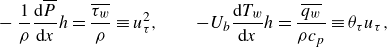
The values of HR, DR and the difference ${\textrm{HR}} - {\textrm{DR}}$
are shown in figure 5. For all cases considered, HR and DR initially increase with the frequency of forcing, but for
${\textrm{HR}} - {\textrm{DR}}$
are shown in figure 5. For all cases considered, HR and DR initially increase with the frequency of forcing, but for $ \omega ^+ \gtrsim 0.04$
, they reach a maximum value before slowly decreasing at higher frequencies. The maximum DR is approximately
$ \omega ^+ \gtrsim 0.04$
, they reach a maximum value before slowly decreasing at higher frequencies. The maximum DR is approximately $30\,\%$
for all Prandtl numbers, but the maximum HR increases from 30 % to approximately
$30\,\%$
for all Prandtl numbers, but the maximum HR increases from 30 % to approximately $40\,\%$
with increasing Prandtl number, marking a significant disparity between DR and HR. The increasing disparity towards
$40\,\%$
with increasing Prandtl number, marking a significant disparity between DR and HR. The increasing disparity towards ${\textrm{HR}} \gt {\textrm{DR}}$
occurs for
${\textrm{HR}} \gt {\textrm{DR}}$
occurs for $\omega ^+ \ge 0.04$
, however, at
$\omega ^+ \ge 0.04$
, however, at $\omega ^+ = 0.022$
,
$\omega ^+ = 0.022$
, ${\textrm{HR}} \lesssim{\textrm{DR}}$
. The comparison between the reduced-domain results (filled squares) and the full-domain results (open circles) supports the reliability of the production runs. At
${\textrm{HR}} \lesssim{\textrm{DR}}$
. The comparison between the reduced-domain results (filled squares) and the full-domain results (open circles) supports the reliability of the production runs. At $Pr= 7.5$
, the reduced-domain grid is more than twice as coarse as the full-domain grid, yet there is less than
$Pr= 7.5$
, the reduced-domain grid is more than twice as coarse as the full-domain grid, yet there is less than $2\,\%$
difference in DR and HR (Appendix A gives more details). The trends in DR seen here have been widely recorded in the previous literature, as the review by Ricco et al. (Reference Ricco, Skote and Leschziner2021) makes clear. However, to the best of the authors’ knowledge, the behaviour of HR has not been reported before. In § 3.4 we relate the observed trends between HR and DR to the attenuation in the turbulent shear stress
$2\,\%$
difference in DR and HR (Appendix A gives more details). The trends in DR seen here have been widely recorded in the previous literature, as the review by Ricco et al. (Reference Ricco, Skote and Leschziner2021) makes clear. However, to the best of the authors’ knowledge, the behaviour of HR has not been reported before. In § 3.4 we relate the observed trends between HR and DR to the attenuation in the turbulent shear stress $\overline {uv}$
and turbulent scalar flux
$\overline {uv}$
and turbulent scalar flux $\overline {\theta v}$
, followed by studying their interactions with the Stokes layer (§ 3.6--3.8).
$\overline {\theta v}$
, followed by studying their interactions with the Stokes layer (§ 3.6--3.8).
Values of ${\textrm{DR}}\,\%$
(blue symbols),
${\textrm{DR}}\,\%$
(blue symbols), ${\textrm{HR}}\,\%$
(red symbols) and their difference (black symbols) for the cases given in table 1. Filled squares: reduced-domain simulations; empty circles: full-domain simulations. Blue dashed line marks the maximum DR; red dashed-dotted line marks the maximum HR.
${\textrm{HR}}\,\%$
(red symbols) and their difference (black symbols) for the cases given in table 1. Filled squares: reduced-domain simulations; empty circles: full-domain simulations. Blue dashed line marks the maximum DR; red dashed-dotted line marks the maximum HR.
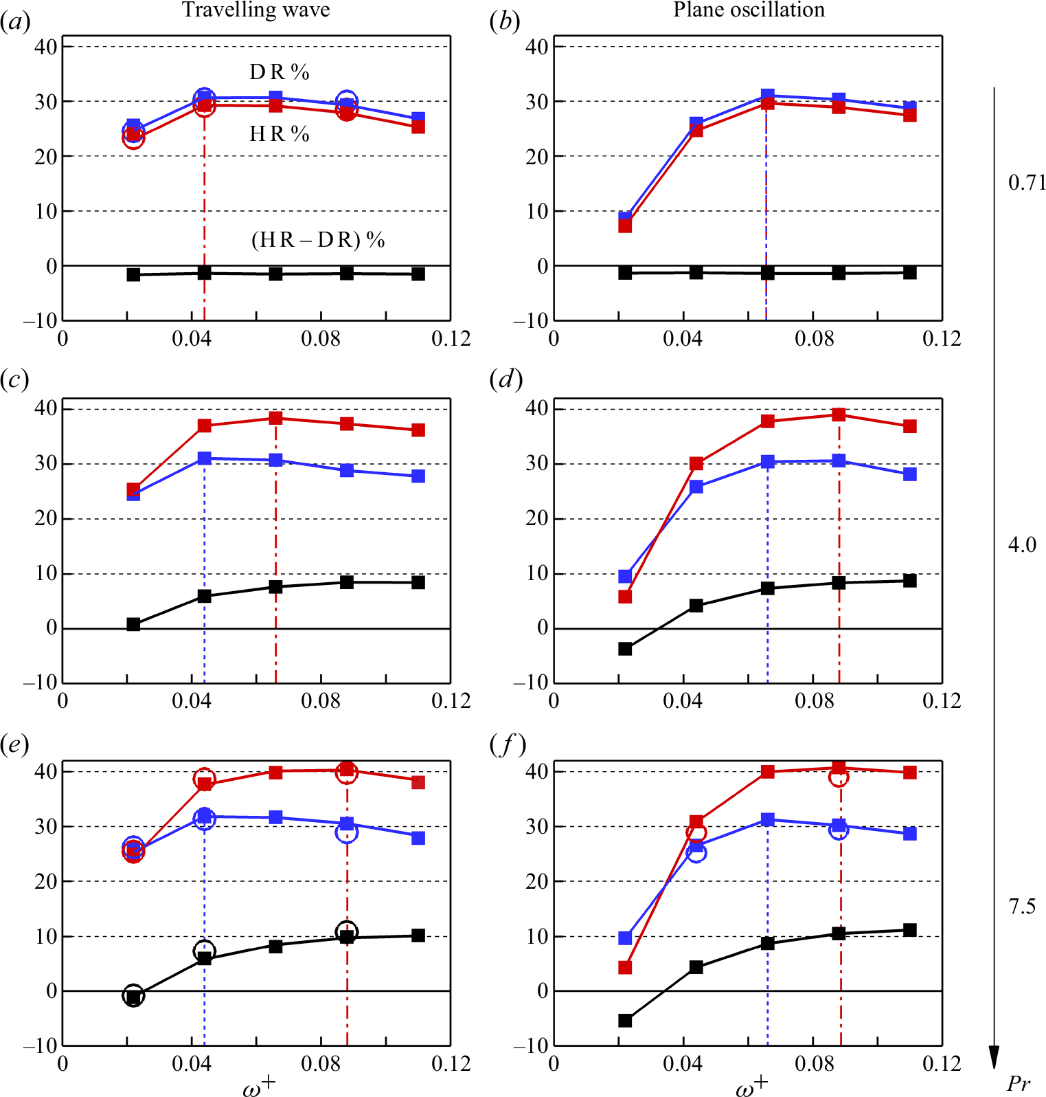
Plane oscillation data of ${\textrm{DR}}\,\%$
(blue symbols) and
${\textrm{DR}}\,\%$
(blue symbols) and ${\textrm{HR}}\,\%$
(orange/red symbols) at
${\textrm{HR}}\,\%$
(orange/red symbols) at $Pr = 0.7 - 1.0$
from our present study, Guérin et al. (Reference Guérin, Flageul, Cordier, Grieu and Agostini2024), and Fang et al. (Reference Fang, Lu and Shao2009).
$Pr = 0.7 - 1.0$
from our present study, Guérin et al. (Reference Guérin, Flageul, Cordier, Grieu and Agostini2024), and Fang et al. (Reference Fang, Lu and Shao2009).
In figure 6 we plot the plane oscillation data of DR and HR at close $Pr = 0.71 - 1.0$
from our present study (figure 5
b), Guérin et al. (Reference Guérin, Flageul, Cordier, Grieu and Agostini2024) and Fang et al. (Reference Fang, Lu and Shao2009). Unlike our data, the two cited studies obtain heat transfer increase (
$Pr = 0.71 - 1.0$
from our present study (figure 5
b), Guérin et al. (Reference Guérin, Flageul, Cordier, Grieu and Agostini2024) and Fang et al. (Reference Fang, Lu and Shao2009). Unlike our data, the two cited studies obtain heat transfer increase ( ${\textrm{HR}} \lesssim 0$
). Compared with Guérin et al. (Reference Guérin, Flageul, Cordier, Grieu and Agostini2024), our
${\textrm{HR}} \lesssim 0$
). Compared with Guérin et al. (Reference Guérin, Flageul, Cordier, Grieu and Agostini2024), our $A^+$
values differ by
$A^+$
values differ by $2.5$
times and
$2.5$
times and $\omega ^+$
values differ by
$\omega ^+$
values differ by $1.7$
times. Nevertheless, based on our findings from §§ 3.6to 3.8, we speculate that
$1.7$
times. Nevertheless, based on our findings from §§ 3.6to 3.8, we speculate that ${\textrm{HR}} \lt {\textrm{DR}} \lt 0$
by Reference Guérin, Flageul, Cordier, Grieu and AgostiniGuérin et al. (2024) is related to the highly protrusive Stokes layer (beyond
${\textrm{HR}} \lt {\textrm{DR}} \lt 0$
by Reference Guérin, Flageul, Cordier, Grieu and AgostiniGuérin et al. (2024) is related to the highly protrusive Stokes layer (beyond $50$
viscous units) for
$50$
viscous units) for $\omega ^+ \lt 0.04$
(figure 22). Compared with Fang et al. (Reference Fang, Lu and Shao2009), we have close values of
$\omega ^+ \lt 0.04$
(figure 22). Compared with Fang et al. (Reference Fang, Lu and Shao2009), we have close values of $A^+$
and
$A^+$
and $\omega ^+$
. At
$\omega ^+$
. At $A^+ \simeq 12.0$
and
$A^+ \simeq 12.0$
and $\omega ^+\simeq 0.06$
, the DR values differ by
$\omega ^+\simeq 0.06$
, the DR values differ by $9\,\%$
between Fang et al. (Reference Fang, Lu and Shao2009) (
$9\,\%$
between Fang et al. (Reference Fang, Lu and Shao2009) ( ${\textrm{DR}} = 40\,\%$
,
${\textrm{DR}} = 40\,\%$
, $Re_{\tau _0} = 180$
) and our study (
$Re_{\tau _0} = 180$
) and our study ( ${\textrm{DR}} = 31\,\%$
at
${\textrm{DR}} = 31\,\%$
at $Re_{\tau _0} = 590$
); this is due to the Reynolds number difference, as discussed in the literature (Gatti & Quadrio Reference Gatti and Quadrio2016; Marusic et al. Reference Marusic, Chandran, Rouhi, Fu, Wine, Holloway, Chung and Smits2021; Rouhi et al. 2023). However, the values of HRhave opposite signs and are different by
$Re_{\tau _0} = 590$
); this is due to the Reynolds number difference, as discussed in the literature (Gatti & Quadrio Reference Gatti and Quadrio2016; Marusic et al. Reference Marusic, Chandran, Rouhi, Fu, Wine, Holloway, Chung and Smits2021; Rouhi et al. 2023). However, the values of HRhave opposite signs and are different by $80\,\%$
,
$80\,\%$
, ${\textrm{HR}} = 30\,\%$
from our study versus
${\textrm{HR}} = 30\,\%$
from our study versus ${\textrm{HR}} = -50\,\%$
from Fang et al. (Reference Fang, Lu and Shao2009). In addition to
${\textrm{HR}} = -50\,\%$
from Fang et al. (Reference Fang, Lu and Shao2009). In addition to $Re_{\tau _0}$
, we speculate that such a difference is related to the different computational set-ups. We conduct DNS of incompressible turbulent channel flow with
$Re_{\tau _0}$
, we speculate that such a difference is related to the different computational set-ups. We conduct DNS of incompressible turbulent channel flow with $\unicode{x1D6E5} ^+_x \times \unicode{x1D6E5} ^+_z = 8.3 \times 3.9$
, while Fang et al. (Reference Fang, Lu and Shao2009) conduct large-eddy simulation (LES) of compressible turbulent channel flow (Mach number
$\unicode{x1D6E5} ^+_x \times \unicode{x1D6E5} ^+_z = 8.3 \times 3.9$
, while Fang et al. (Reference Fang, Lu and Shao2009) conduct large-eddy simulation (LES) of compressible turbulent channel flow (Mach number $Ma = 0.5$
) with
$Ma = 0.5$
) with $\unicode{x1D6E5} ^+_x \times \unicode{x1D6E5} ^+_z = 35 \times 12$
.
$\unicode{x1D6E5} ^+_x \times \unicode{x1D6E5} ^+_z = 35 \times 12$
.
3.2. Optimal actuation frequency
Figure 5 indicates that for the considered cases, the optimal actuation frequency for DR is $\omega ^+ \approx 0.044$
for the travelling wave and
$\omega ^+ \approx 0.044$
for the travelling wave and $\approx 0.066$
for the plane oscillation, regardless of the Prandtl number. For HR, the optimal frequency coincides with that for DR at
$\approx 0.066$
for the plane oscillation, regardless of the Prandtl number. For HR, the optimal frequency coincides with that for DR at $Pr = 0.71$
, but it increases to
$Pr = 0.71$
, but it increases to $0.088$
for both types of actuation as the Prandtl number increases to 7.5.
$0.088$
for both types of actuation as the Prandtl number increases to 7.5.
Previous studies relate the optimal frequency for DR to the characteristic time scale of the energetic velocity scales associated with the near-wall cycle of turbulence, $\mathcal{T}^+_u$
(Quadrio et al. Reference Quadrio, Ricco and Viotti2009; Chandran et al. Reference Chandran, Zampiron, Rouhi, Fu, Wine, Holloway, Smits and Marusic2023). When the actuation period
$\mathcal{T}^+_u$
(Quadrio et al. Reference Quadrio, Ricco and Viotti2009; Chandran et al. Reference Chandran, Zampiron, Rouhi, Fu, Wine, Holloway, Smits and Marusic2023). When the actuation period $T^+_{osc} \equiv 2 \pi /\omega ^+$
matches this time scale, the wall oscillation becomes more effective in disrupting the near-wall scales, leading to the maximum DR (Ricco et al. Reference Ricco, Skote and Leschziner2021). Chandran et al. (Reference Chandran, Zampiron, Rouhi, Fu, Wine, Holloway, Smits and Marusic2023) discuss this interaction using the pre-multiplied spectrum of wall shear stress
$T^+_{osc} \equiv 2 \pi /\omega ^+$
matches this time scale, the wall oscillation becomes more effective in disrupting the near-wall scales, leading to the maximum DR (Ricco et al. Reference Ricco, Skote and Leschziner2021). Chandran et al. (Reference Chandran, Zampiron, Rouhi, Fu, Wine, Holloway, Smits and Marusic2023) discuss this interaction using the pre-multiplied spectrum of wall shear stress $f^+ \phi ^+_{\tau \tau }$
, and the corresponding spectra for our non-actuated case are shown in figure 7(a–c) (blue lines). In agreement with Chandran et al. (Reference Chandran, Zampiron, Rouhi, Fu, Wine, Holloway, Smits and Marusic2023), the peaks in the shear stress spectra occur at
$f^+ \phi ^+_{\tau \tau }$
, and the corresponding spectra for our non-actuated case are shown in figure 7(a–c) (blue lines). In agreement with Chandran et al. (Reference Chandran, Zampiron, Rouhi, Fu, Wine, Holloway, Smits and Marusic2023), the peaks in the shear stress spectra occur at $\mathcal{T}^+_u \simeq 100$
, corresponding to
$\mathcal{T}^+_u \simeq 100$
, corresponding to $\omega ^+ \simeq 0.063$
, which broadly matches the frequencies of actuation for maximum DR found here.
$\omega ^+ \simeq 0.063$
, which broadly matches the frequencies of actuation for maximum DR found here.
Non-actuated half-channel flow with increasing Prandtl number: (a,d,g) $Pr = 0.71$
, (b,e,h)
$Pr = 0.71$
, (b,e,h) $Pr = 4.0$
, (c,f,i)
$Pr = 4.0$
, (c,f,i) $Pr = 7.5$
. (a–c) Pre-multiplied frequency spectra of wall shear stress
$Pr = 7.5$
. (a–c) Pre-multiplied frequency spectra of wall shear stress $f^+ \phi ^+_{\tau \tau }$
(blue line) and wall heat flux
$f^+ \phi ^+_{\tau \tau }$
(blue line) and wall heat flux $f^+ \phi ^+_{qq}$
(red line), where
$f^+ \phi ^+_{qq}$
(red line), where $T^+ = 1/f^+$
. (d–f) Spectrograms of the streamwise velocity fluctuations (blue contour lines) and temperature fluctuations (filled contour) pre-multiplied by the spanwise wavenumber
$T^+ = 1/f^+$
. (d–f) Spectrograms of the streamwise velocity fluctuations (blue contour lines) and temperature fluctuations (filled contour) pre-multiplied by the spanwise wavenumber $k^+_z$
. (g–i) Same as (d–f), pre-multiplied by the streamwise wavenumber
$k^+_z$
. (g–i) Same as (d–f), pre-multiplied by the streamwise wavenumber $k^+_x$
. Contour levels for
$k^+_x$
. Contour levels for $k^+_z \phi ^+_{u u}$
start from
$k^+_z \phi ^+_{u u}$
start from $0.2$
to
$0.2$
to $3.8$
with an increment of
$3.8$
with an increment of $0.6$
; contour levels for
$0.6$
; contour levels for $k^+_x \phi ^+_{u u}$
start from
$k^+_x \phi ^+_{u u}$
start from $0.2$
to
$0.2$
to $2.2$
with an increment of
$2.2$
with an increment of $0.4$
. The blue and red bullets in (d–f) locate the maximum in
$0.4$
. The blue and red bullets in (d–f) locate the maximum in $k^+_z \phi ^+_{u u}$
and
$k^+_z \phi ^+_{u u}$
and $k^+_z \phi ^+_{\theta \theta }$
, respectively, and in (g–i) locate the maximum in
$k^+_z \phi ^+_{\theta \theta }$
, respectively, and in (g–i) locate the maximum in $k^+_x \phi ^+_{u u}$
and
$k^+_x \phi ^+_{u u}$
and $k^+_x \phi ^+_{\theta \theta }$
, respectively.
$k^+_x \phi ^+_{\theta \theta }$
, respectively.

Figure 7 also shows the corresponding spectra for the fluctuating wall heat flux, $f^+ \phi ^+_{qq}$
(red lines), as well as the pre-multiplied spectrograms of the fluctuating streamwise velocity and temperature (
$f^+ \phi ^+_{qq}$
(red lines), as well as the pre-multiplied spectrograms of the fluctuating streamwise velocity and temperature ( $k^+_z \phi ^+_{uu}, \ k^+_x \phi ^+_{uu}, \ k^+_z \phi ^+_{\theta \theta }, \ k^+_x \phi ^+_{\theta \theta }$
). Figure 7(a,b,c) reveals that while
$k^+_z \phi ^+_{uu}, \ k^+_x \phi ^+_{uu}, \ k^+_z \phi ^+_{\theta \theta }, \ k^+_x \phi ^+_{\theta \theta }$
). Figure 7(a,b,c) reveals that while $f^+ \phi ^+_{qq}$
is sensitive to
$f^+ \phi ^+_{qq}$
is sensitive to $Pr$
at small time scales (
$Pr$
at small time scales ( $T^+ \lesssim 70$
), the time scale of the energetic temperature scales
$T^+ \lesssim 70$
), the time scale of the energetic temperature scales $\mathcal{T}^+_\theta \simeq 100$
is insensitive to
$\mathcal{T}^+_\theta \simeq 100$
is insensitive to $Pr$
, and coincides with
$Pr$
, and coincides with $\mathcal{T}^+_u$
. The streamwise and spanwise lengths of the energetic temperature scales vary somewhat with Prandtl number (see figure 7
d–i), but they also remain close to the length scales of the energetic velocity scales. However, the peak in
$\mathcal{T}^+_u$
. The streamwise and spanwise lengths of the energetic temperature scales vary somewhat with Prandtl number (see figure 7
d–i), but they also remain close to the length scales of the energetic velocity scales. However, the peak in $k^+_z \phi ^+_{\theta \theta }$
drops from
$k^+_z \phi ^+_{\theta \theta }$
drops from $y^+ = 16$
at
$y^+ = 16$
at $Pr = 0.71$
to
$Pr = 0.71$
to $y^+ = 5$
at
$y^+ = 5$
at $Pr = 7.5$
, as the conductive sublayer thins with increasing Prandtl number (Alcántara-Á vila & Hoyas Reference Alcántara-Á vila and Hoyas2021; Kader Reference Kader1981; Schwertfirm & Manhart Reference Schwertfirm and Manhart2007). The
$Pr = 7.5$
, as the conductive sublayer thins with increasing Prandtl number (Alcántara-Á vila & Hoyas Reference Alcántara-Á vila and Hoyas2021; Kader Reference Kader1981; Schwertfirm & Manhart Reference Schwertfirm and Manhart2007). The $y^+$
location of the peak in
$y^+$
location of the peak in $k^+_z \phi ^+_{\theta \theta }$
scales with approximately
$k^+_z \phi ^+_{\theta \theta }$
scales with approximately $ Pr^{-1/2}$
, which is steeper than the scaling of approximately
$ Pr^{-1/2}$
, which is steeper than the scaling of approximately $ Pr^{-1/3}$
for the conductive sublayer thickness for
$ Pr^{-1/3}$
for the conductive sublayer thickness for $Pr \gtrsim 1$
(Shaw & Hanratty Reference Shaw and Hanratty1977; Kader Reference Kader1981; Schwertfirm & Manhart Reference Schwertfirm and Manhart2007; Alcántara-Á vila & Hoyas Reference Alcántara-Á vila and Hoyas2021; Pirozzoli Reference Pirozzoli2023). We also analysed the
$Pr \gtrsim 1$
(Shaw & Hanratty Reference Shaw and Hanratty1977; Kader Reference Kader1981; Schwertfirm & Manhart Reference Schwertfirm and Manhart2007; Alcántara-Á vila & Hoyas Reference Alcántara-Á vila and Hoyas2021; Pirozzoli Reference Pirozzoli2023). We also analysed the $\overline {\theta ^2}^+$
profiles of Pirozzoli (Reference Pirozzoli2023) for the DNS of the turbulent pipe flow at
$\overline {\theta ^2}^+$
profiles of Pirozzoli (Reference Pirozzoli2023) for the DNS of the turbulent pipe flow at $Re_{\tau _0} \simeq 1100$
and
$Re_{\tau _0} \simeq 1100$
and $Pr = 0.5, 1, 2, 4, 16$
, and the
$Pr = 0.5, 1, 2, 4, 16$
, and the $y^+$
locations of their inner peaks scale with approximately
$y^+$
locations of their inner peaks scale with approximately $ Pr^{-1/2}$
.
$ Pr^{-1/2}$
.
For the plane oscillation, we expect that the maximum DR and HR is achieved when the actuation period is close to $\mathcal{T}^+_u$
and
$\mathcal{T}^+_u$
and $\mathcal{T}^+_\theta$
, respectively. For the travelling wave, however, the optimal actuation period cannot be directly compared with
$\mathcal{T}^+_\theta$
, respectively. For the travelling wave, however, the optimal actuation period cannot be directly compared with $\mathcal{T}^+_u$
or
$\mathcal{T}^+_u$
or $\mathcal{T}^+_\theta$
, owing to the relative streamwise motion between the travelling wave and the advecting near-wall scales. As discussed by Quadrio et al. (Reference Quadrio, Ricco and Viotti2009), for maximum DR,
$\mathcal{T}^+_\theta$
, owing to the relative streamwise motion between the travelling wave and the advecting near-wall scales. As discussed by Quadrio et al. (Reference Quadrio, Ricco and Viotti2009), for maximum DR, $\mathcal{T}^+_u$
must be compared with a relative oscillation period
$\mathcal{T}^+_u$
must be compared with a relative oscillation period $2\pi /(\kappa ^+_x \mathcal{U}^+_u + \omega ^+)$
as seen by an observer travelling with the convection speed of the near-wall energetic velocity scales
$2\pi /(\kappa ^+_x \mathcal{U}^+_u + \omega ^+)$
as seen by an observer travelling with the convection speed of the near-wall energetic velocity scales $\mathcal{U}^+_u$
. Similarly, for maximum HR,
$\mathcal{U}^+_u$
. Similarly, for maximum HR, $\mathcal{T}^+_\theta$
must be compared with
$\mathcal{T}^+_\theta$
must be compared with $2\pi /(\kappa ^+_x \mathcal{U}^+_\theta + \omega ^+)$
, where
$2\pi /(\kappa ^+_x \mathcal{U}^+_\theta + \omega ^+)$
, where $\mathcal{U}^+_\theta$
is the convection speed of the near-wall energetic temperature scales. After some recasting (using
$\mathcal{U}^+_\theta$
is the convection speed of the near-wall energetic temperature scales. After some recasting (using $\mathcal{T}^+_u \simeq \mathcal{T}^+_\theta \simeq 100$
,
$\mathcal{T}^+_u \simeq \mathcal{T}^+_\theta \simeq 100$
, $\kappa ^+_x = 0.0014$
), we estimate the optimum frequencies of actuation for DR and HR to be, respectively,
$\kappa ^+_x = 0.0014$
), we estimate the optimum frequencies of actuation for DR and HR to be, respectively,
 \begin{align} &\qquad\omega ^+_{\textrm{opt}, {\textrm{DR}}} = \frac {2\pi }{\mathcal{T}^+_u} - \kappa ^+_x \mathcal{U}^+_u \simeq 0.046, \end{align}
 \begin{align} &\omega ^+_{\textrm{opt}, {\textrm{HR}}} = \frac {2\pi }{\mathcal{T}^+_\theta } - \kappa ^+_x \mathcal{U}^+_\theta \simeq 0.063 - 0.0014 \mathcal{U}^+_\theta, \end{align}
where we have assumed that $\mathcal{U}^+_u$
follows a universal curve (Kim & Hussain Reference Kim and Hussain1993; Del Á lamo & Jiménez Reference Del Á. lamo and Jiménez2009; Liu & Gayme Reference Liu and Gayme2020), where
$\mathcal{U}^+_u$
follows a universal curve (Kim & Hussain Reference Kim and Hussain1993; Del Á lamo & Jiménez Reference Del Á. lamo and Jiménez2009; Liu & Gayme Reference Liu and Gayme2020), where $\mathcal{U}^+_u \simeq 12$
at
$\mathcal{U}^+_u \simeq 12$
at $y^+ \simeq 15$
(marked with blue bullets in figure 7
d–i).
$y^+ \simeq 15$
(marked with blue bullets in figure 7
d–i).
The estimated optimum frequency for DR is independent of Prandtl number, at approximately $0.046$
, consistent with our DNS results for the travelling wave case (figure 5
a,c,e). However, the optimum frequency for HR depends on
$0.046$
, consistent with our DNS results for the travelling wave case (figure 5
a,c,e). However, the optimum frequency for HR depends on $Pr$
, since we expect that
$Pr$
, since we expect that $\mathcal{U}^+_\theta$
decreases as the energetic temperature scales move closer to the wall with increasing Prandtl number (red bullets in figure 7
d–i). Hetsroni et al. (Reference Hetsroni, Tiselj, Bergant, Mosyak and Pogrebnyak2004) computed the profiles of
$\mathcal{U}^+_\theta$
decreases as the energetic temperature scales move closer to the wall with increasing Prandtl number (red bullets in figure 7
d–i). Hetsroni et al. (Reference Hetsroni, Tiselj, Bergant, Mosyak and Pogrebnyak2004) computed the profiles of $\mathcal{U}^+_\theta$
at
$\mathcal{U}^+_\theta$
at $Pr = 1.0$
, 5.4 and 54 in a configuration similar to that used in the present study, without actuation. Using their results, we estimate that
$Pr = 1.0$
, 5.4 and 54 in a configuration similar to that used in the present study, without actuation. Using their results, we estimate that $\mathcal{U}^+_\theta$
decreases from
$\mathcal{U}^+_\theta$
decreases from $12$
to
$12$
to $6$
as
$6$
as $Pr$
increases from
$Pr$
increases from $0.71$
to
$0.71$
to $7.5$
, which gives
$7.5$
, which gives $\omega ^+_{\textrm{opt},{\textrm{HR}}} = 0.046$
at
$\omega ^+_{\textrm{opt},{\textrm{HR}}} = 0.046$
at $Pr = 0.71$
and
$Pr = 0.71$
and $0.055$
at
$0.055$
at $Pr = 7.5$
. The estimated value at
$Pr = 7.5$
. The estimated value at $Pr = 7.5$
is smaller than the value of 0.088 given by the DNS (figure 5
e), but the trends with Prandtl number are consistent. In §§ 3.6 and 3.7 we conduct a more quantitative justification for the trends in
$Pr = 7.5$
is smaller than the value of 0.088 given by the DNS (figure 5
e), but the trends with Prandtl number are consistent. In §§ 3.6 and 3.7 we conduct a more quantitative justification for the trends in $\omega ^+_{{opt},{\textrm{HR}}}$
by considering the interaction between the Stokes layer and the near-wall thermal field.
$\omega ^+_{{opt},{\textrm{HR}}}$
by considering the interaction between the Stokes layer and the near-wall thermal field.
Travelling wave actuation with $A^+ = 12$
,
$A^+ = 12$
, $\kappa ^+_x = 0.0014$
. Left column:
$\kappa ^+_x = 0.0014$
. Left column: ${\textrm{DR}}\,\%$
and
${\textrm{DR}}\,\%$
and $\overline {U}^*$
profiles, where
$\overline {U}^*$
profiles, where $\unicode{x1D6E5} \overline {U}^* = \overline {U}^* - \overline {U}^*_0$
(results independent of
$\unicode{x1D6E5} \overline {U}^* = \overline {U}^* - \overline {U}^*_0$
(results independent of $Pr$
). Middle and right columns correspond to
$Pr$
). Middle and right columns correspond to $Pr=0.71$
and
$Pr=0.71$
and $7.5$
, respectively:
$7.5$
, respectively: ${\textrm{DR}}\,\%$
(blue line),
${\textrm{DR}}\,\%$
(blue line), ${\textrm{HR}}\,\%$
(red line) and
${\textrm{HR}}\,\%$
(red line) and $\overline {\Theta }^*$
profiles, where
$\overline {\Theta }^*$
profiles, where $\unicode{x1D6E5} \overline {\Theta }^* = \Theta ^* - \Theta ^*_0$
. In the panels (d–i) the black line is the reference (non-actuated) case, the blue and red lines show the effects of increasing
$\unicode{x1D6E5} \overline {\Theta }^* = \Theta ^* - \Theta ^*_0$
. In the panels (d–i) the black line is the reference (non-actuated) case, the blue and red lines show the effects of increasing $\omega ^+$
on
$\omega ^+$
on $\overline {U}^*$
and
$\overline {U}^*$
and $\overline {\Theta ^*}$
, respectively, and the thick dashed line corresponds to
$\overline {\Theta ^*}$
, respectively, and the thick dashed line corresponds to ${\textrm{DR}}_{{max}}$
or
${\textrm{DR}}_{{max}}$
or ${\textrm{HR}}_{{max}}$
. In (d,e,f) the thin dotted lines for
${\textrm{HR}}_{{max}}$
. In (d,e,f) the thin dotted lines for $y^* \gtrsim 170$
are the reconstructed profiles following § 2.3. In (j,k,l) we plot the reduced-domain profiles (red/blue) up to
$y^* \gtrsim 170$
are the reconstructed profiles following § 2.3. In (j,k,l) we plot the reduced-domain profiles (red/blue) up to $y^*_{{res}} \simeq 170$
, and the thick grey profiles are from the full-domain cases (
$y^*_{{res}} \simeq 170$
, and the thick grey profiles are from the full-domain cases ( $L_x \times L_z = 7.6 h \times \pi h$
) from Appendix A; the dashed-dotted green profile in (j) is at matched
$L_x \times L_z = 7.6 h \times \pi h$
) from Appendix A; the dashed-dotted green profile in (j) is at matched $A^+ = 12, \kappa ^+_x = 0.0014, \omega ^+ = 0.044$
but at
$A^+ = 12, \kappa ^+_x = 0.0014, \omega ^+ = 0.044$
but at $Re_{\tau _0} = 950$
from Rouhi et al. (Reference Rouhi, Fu, Chandran, Zampiron, Smits and Marusic2023). The black cross symbols mark the distance
$Re_{\tau _0} = 950$
from Rouhi et al. (Reference Rouhi, Fu, Chandran, Zampiron, Smits and Marusic2023). The black cross symbols mark the distance $y^*$
where
$y^*$
where $\unicode{x1D6E5} \overline {U}^* = 0.9 \unicode{x1D6E5} \overline {U}^*_{170}$
(
$\unicode{x1D6E5} \overline {U}^* = 0.9 \unicode{x1D6E5} \overline {U}^*_{170}$
( $\unicode{x1D6E5} \overline {\Theta }^* = 0.9 \unicode{x1D6E5} \overline {\Theta }^*_{170}$
).
$\unicode{x1D6E5} \overline {\Theta }^* = 0.9 \unicode{x1D6E5} \overline {\Theta }^*_{170}$
).
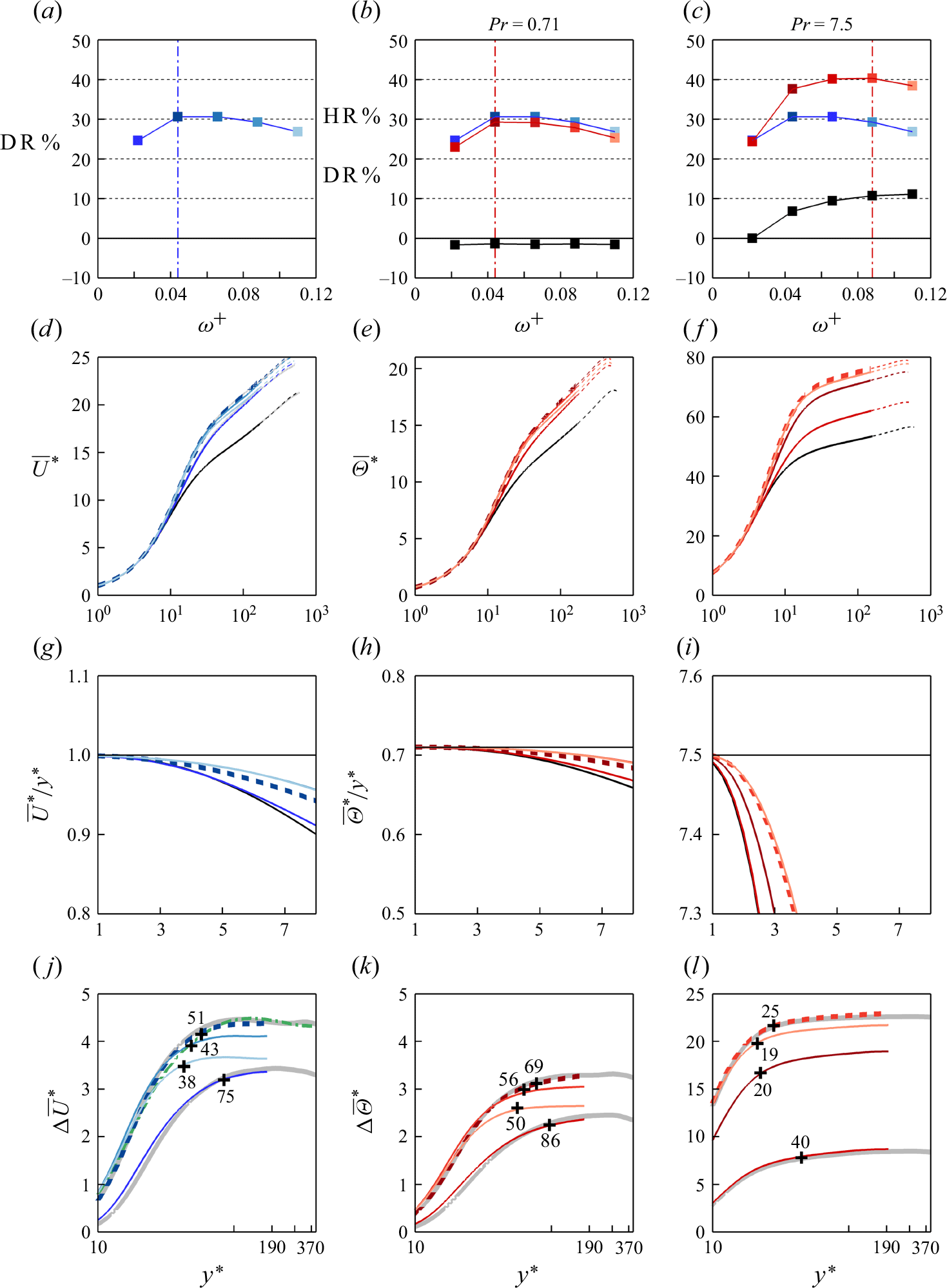
Travelling wave actuation with $A^+ = 12$
,
$A^+ = 12$
, $\kappa ^+_x = 0.0014$
. Notation and symbols as in figure 8. Here,
$\kappa ^+_x = 0.0014$
. Notation and symbols as in figure 8. Here, $\unicode{x1D6E5} \overline { u v}^* = \overline { u v }^* - \overline { u v }^*_0$
and
$\unicode{x1D6E5} \overline { u v}^* = \overline { u v }^* - \overline { u v }^*_0$
and $\unicode{x1D6E5} \overline { \theta v }^* = \overline { \theta v }^* - \overline { \theta v }^*_0$
. In (d,e,f) the numbers give the
$\unicode{x1D6E5} \overline { \theta v }^* = \overline { \theta v }^* - \overline { \theta v }^*_0$
. In (d,e,f) the numbers give the $y^*$
location of the inner peak in the
$y^*$
location of the inner peak in the $\overline { u^2 }^*$
and
$\overline { u^2 }^*$
and $\overline {\theta ^2 }^*$
profiles. In (g–l) the vertical dashed line locates the peak of non-actuated
$\overline {\theta ^2 }^*$
profiles. In (g–l) the vertical dashed line locates the peak of non-actuated $\overline { u v }^*_0$
(g,j) and
$\overline { u v }^*_0$
(g,j) and $\overline { \theta v }^*_0$
(h,i,k,l).
$\overline { \theta v }^*_0$
(h,i,k,l).
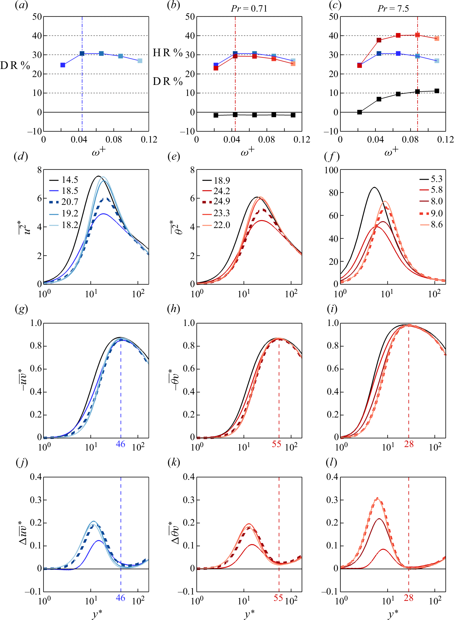
3.3. Mean profiles and turbulence statistics
We now consider the distributions of the mean velocity $\overline {U}^*$
(
$\overline {U}^*$
( $=\overline {U}/u_\tau$
), the mean temperature
$=\overline {U}/u_\tau$
), the mean temperature $\overline {\Theta }^*$
(
$\overline {\Theta }^*$
( $= \overline {\Theta }/\theta _\tau$
) (figure 8), and the velocity and temperature statistics (figure 9) as we vary
$= \overline {\Theta }/\theta _\tau$
) (figure 8), and the velocity and temperature statistics (figure 9) as we vary $\omega ^+$
and
$\omega ^+$
and $Pr$
. We focus on the travelling wave case, but since the observed trends are consistent with those from the plane oscillation case (figures 28 and 29 in Appendix C), our conclusions are applicable to both types of actuation.
$Pr$
. We focus on the travelling wave case, but since the observed trends are consistent with those from the plane oscillation case (figures 28 and 29 in Appendix C), our conclusions are applicable to both types of actuation.
It is well known from the literature that DR by either plane oscillation or a travelling wave coincides with the thickening of the viscous sublayer (Choi et al. Reference Choi, DeBisschop and Clayton1998; Choi & Clayton Reference Choi and Clayton2001; Choi Reference Choi2002; Di Cicca et al. Reference Di Cicca, Iuso, Spazzini and Onorato2002; Touber & Leschziner Reference Touber and Leschziner2012; Hurst et al. Reference Hurst, Yang and Chung2014; Gatti & Quadrio Reference Gatti and Quadrio2016; Chandran et al. Reference Chandran, Zampiron, Rouhi, Fu, Wine, Holloway, Smits and Marusic2023; Rouhi et al. Reference Rouhi, Fu, Chandran, Zampiron, Smits and Marusic2023). This is evident also from our $\overline {U}^*/y^*$
profiles (figure 8
g), where the actuated profiles (blue profiles) depart from unity farther from the wall compared with the non-actuated profile (black profile). The conductive sublayer also thickens with wall oscillation, but it then thins substantially with increasing Prandtl number, so that at
$\overline {U}^*/y^*$
profiles (figure 8
g), where the actuated profiles (blue profiles) depart from unity farther from the wall compared with the non-actuated profile (black profile). The conductive sublayer also thickens with wall oscillation, but it then thins substantially with increasing Prandtl number, so that at $Pr = 7.5$
the conductive sublayer is substantially thinner than the viscous sublayer (figure 8
i).
$Pr = 7.5$
the conductive sublayer is substantially thinner than the viscous sublayer (figure 8
i).
Viscous sublayer and conductive sublayer thickening due to the wall oscillation shifts the $\overline {U}^*$
and
$\overline {U}^*$
and $\overline {\Theta }^*$
profiles. This is shown in figure 8(j,k,l) where we plot the differences
$\overline {\Theta }^*$
profiles. This is shown in figure 8(j,k,l) where we plot the differences $\unicode{x1D6E5} \overline {U}^* = \overline {U}^* - \overline {U}^*_0$
and
$\unicode{x1D6E5} \overline {U}^* = \overline {U}^* - \overline {U}^*_0$
and $\unicode{x1D6E5} \overline {\Theta }^* = \overline {\Theta }^* - \overline {\Theta }^*_0$
between the actuated and non-actuated cases. The cases with the maximum DR (or HR) have the highest
$\unicode{x1D6E5} \overline {\Theta }^* = \overline {\Theta }^* - \overline {\Theta }^*_0$
between the actuated and non-actuated cases. The cases with the maximum DR (or HR) have the highest $\unicode{x1D6E5} \overline {U}^*$
(or
$\unicode{x1D6E5} \overline {U}^*$
(or $\unicode{x1D6E5} \overline {\Theta }^*$
), as highlighted by the thick dashed line in the plots. The profiles in colour are from the production runs with the reduced domain (table 1), and are plotted up to
$\unicode{x1D6E5} \overline {\Theta }^*$
), as highlighted by the thick dashed line in the plots. The profiles in colour are from the production runs with the reduced domain (table 1), and are plotted up to $y^*_{{res}} \simeq 170$
. As a reference, the profiles in grey are from the full-domain cases from Appendix A. There is a good agreement between the reduced-domain and full-domain profiles up to
$y^*_{{res}} \simeq 170$
. As a reference, the profiles in grey are from the full-domain cases from Appendix A. There is a good agreement between the reduced-domain and full-domain profiles up to $y^*_{{res}}$
. Furthermore, the variations of
$y^*_{{res}}$
. Furthermore, the variations of $\unicode{x1D6E5} \overline {U}^*$
and
$\unicode{x1D6E5} \overline {U}^*$
and $\unicode{x1D6E5} \overline {\Theta }^*$
beyond
$\unicode{x1D6E5} \overline {\Theta }^*$
beyond $y^*_{{res}}$
are within
$y^*_{{res}}$
are within $3\,\%$
. Therefore, it is reasonable to consider
$3\,\%$
. Therefore, it is reasonable to consider $\unicode{x1D6E5} \overline {U}^*$
and
$\unicode{x1D6E5} \overline {U}^*$
and $\unicode{x1D6E5} \overline {\Theta }^*$
at
$\unicode{x1D6E5} \overline {\Theta }^*$
at $y^*_{{res}} = 170$
(
$y^*_{{res}} = 170$
( $\unicode{x1D6E5} \overline {U}^*_{170}$
and
$\unicode{x1D6E5} \overline {U}^*_{170}$
and $\unicode{x1D6E5} \overline {\Theta }^*_{170}$
) as their asymptotic values. According to Rouhi et al. (Reference Rouhi, Fu, Chandran, Zampiron, Smits and Marusic2023), the distance
$\unicode{x1D6E5} \overline {\Theta }^*_{170}$
) as their asymptotic values. According to Rouhi et al. (Reference Rouhi, Fu, Chandran, Zampiron, Smits and Marusic2023), the distance $y^*$
where
$y^*$
where $\unicode{x1D6E5} \overline {U}^*$
reaches a plateau indicates the extent to which the Stokes layer disturbs the
$\unicode{x1D6E5} \overline {U}^*$
reaches a plateau indicates the extent to which the Stokes layer disturbs the $\overline {U}^*$
profile. In figure 8(j,k,l), therefore, we mark each profile at the
$\overline {U}^*$
profile. In figure 8(j,k,l), therefore, we mark each profile at the $y^*$
location where
$y^*$
location where $\unicode{x1D6E5} \overline {U}^* = 0.9 \unicode{x1D6E5} \overline {U}^*_{170}$
(
$\unicode{x1D6E5} \overline {U}^* = 0.9 \unicode{x1D6E5} \overline {U}^*_{170}$
( $\unicode{x1D6E5} \overline {\Theta }^* = 0.9 \unicode{x1D6E5} \overline {\Theta }^*_{170}$
). For the present profiles with fixed
$\unicode{x1D6E5} \overline {\Theta }^* = 0.9 \unicode{x1D6E5} \overline {\Theta }^*_{170}$
). For the present profiles with fixed $Re_{\tau _0}, A^+$
and
$Re_{\tau _0}, A^+$
and $\kappa ^+_x$
, the distance to reach the plateau in
$\kappa ^+_x$
, the distance to reach the plateau in $\unicode{x1D6E5} \overline {\Theta }^*$
depends on
$\unicode{x1D6E5} \overline {\Theta }^*$
depends on $\omega ^+$
and
$\omega ^+$
and $Pr$
(compare figures 8
kand
8
l), where the plateau is reached at a lower
$Pr$
(compare figures 8
kand
8
l), where the plateau is reached at a lower $y^*$
with increasing Prandtl number. We expect that the
$y^*$
with increasing Prandtl number. We expect that the $\unicode{x1D6E5} \overline {\Theta }^*$
profiles and the distances to their plateaus would also depend on
$\unicode{x1D6E5} \overline {\Theta }^*$
profiles and the distances to their plateaus would also depend on $A^+$
and
$A^+$
and $\kappa ^+_x$
, but not on
$\kappa ^+_x$
, but not on $Re_{\tau _0}$
. Our conjecture is based on the behaviour of its analogue
$Re_{\tau _0}$
. Our conjecture is based on the behaviour of its analogue $\unicode{x1D6E5} \overline {U}^*$
(figure 8
j) that, for a fixed set of actuation parameters, is almost identical between
$\unicode{x1D6E5} \overline {U}^*$
(figure 8
j) that, for a fixed set of actuation parameters, is almost identical between $Re_{\tau _0} = 590$
(thick blue dashed line) and
$Re_{\tau _0} = 590$
(thick blue dashed line) and $Re_{\tau _0} = 950$
(green dashed-dotted line). The Reynolds number independence of the plateau in
$Re_{\tau _0} = 950$
(green dashed-dotted line). The Reynolds number independence of the plateau in $\unicode{x1D6E5} \overline {U}^*$
for the travelling wave is further confirmed by Gatti & Quadrio (Reference Gatti and Quadrio2016) and Gatti et al. (Reference Gatti, Quadrio, Chiarini, Gattere and Pirozzoli2024).
$\unicode{x1D6E5} \overline {U}^*$
for the travelling wave is further confirmed by Gatti & Quadrio (Reference Gatti and Quadrio2016) and Gatti et al. (Reference Gatti, Quadrio, Chiarini, Gattere and Pirozzoli2024).
In figure 9 we plot the turbulence statistics for the same cases shown in figure 8. Drag reduction and viscous sublayer thickening (figure 8
a,d,g) coincide with the near-wall attenuation of $\overline { u^2}^*$
and the shift in its inner peak (figure 9
d), as known from previous work (Quadrio & Sibilla Reference Quadrio and Sibilla2000; Ricco & Wu Reference Ricco and Wu2004; Quadrio & Ricco Reference Quadrio and Ricco2011; Touber & Leschziner Reference Touber and Leschziner2012; Ricco et al. Reference Ricco, Skote and Leschziner2021; Rouhi et al. Reference Rouhi, Fu, Chandran, Zampiron, Smits and Marusic2023). Similarly, we find that at each
$\overline { u^2}^*$
and the shift in its inner peak (figure 9
d), as known from previous work (Quadrio & Sibilla Reference Quadrio and Sibilla2000; Ricco & Wu Reference Ricco and Wu2004; Quadrio & Ricco Reference Quadrio and Ricco2011; Touber & Leschziner Reference Touber and Leschziner2012; Ricco et al. Reference Ricco, Skote and Leschziner2021; Rouhi et al. Reference Rouhi, Fu, Chandran, Zampiron, Smits and Marusic2023). Similarly, we find that at each $Pr$
, HR and conductive sublayer thickening (figure 8
b,c,e,f,h,i) coincide with the near-wall attenuation of
$Pr$
, HR and conductive sublayer thickening (figure 8
b,c,e,f,h,i) coincide with the near-wall attenuation of $\overline { \theta ^2 }^*$
and the shift in its inner peak (figure 9
e,f). Interestingly,
$\overline { \theta ^2 }^*$
and the shift in its inner peak (figure 9
e,f). Interestingly, ${\textrm{DR}}_{{max}}$
occurs when the inner peak in
${\textrm{DR}}_{{max}}$
occurs when the inner peak in $\overline { u^2}^*$
is located farthest from the wall, and a similar connection exists between
$\overline { u^2}^*$
is located farthest from the wall, and a similar connection exists between ${\textrm{HR}}_{{max}}$
and the location of the inner peak in
${\textrm{HR}}_{{max}}$
and the location of the inner peak in $\overline { \theta ^2}^*$
(compare the listed numbers in figure 9
d,e,f).
$\overline { \theta ^2}^*$
(compare the listed numbers in figure 9
d,e,f).


In addition, the attenuation of the turbulent shear stress $\overline { u v }^*$
(figure 9
g) and the wall-normal turbulent temperature flux
$\overline { u v }^*$
(figure 9
g) and the wall-normal turbulent temperature flux $\overline { \theta v }^*$
(figure 9
h,i) are directly linked to DR and HR, respectively. In figure 9(j,k,l) we plot the differences between the actuated and non-actuated cases
$\overline { \theta v }^*$
(figure 9
h,i) are directly linked to DR and HR, respectively. In figure 9(j,k,l) we plot the differences between the actuated and non-actuated cases $\unicode{x1D6E5} \overline { u v }^* = \overline { u v }^* - \overline { u v }^*_0$
and
$\unicode{x1D6E5} \overline { u v }^* = \overline { u v }^* - \overline { u v }^*_0$
and $\unicode{x1D6E5} \overline { \theta v }^* = \overline { \theta v }^* - \overline { \theta v }^*_0$
. Most of the attenuation occurs near the wall, with the maxima occurring near
$\unicode{x1D6E5} \overline { \theta v }^* = \overline { \theta v }^* - \overline { \theta v }^*_0$
. Most of the attenuation occurs near the wall, with the maxima occurring near $y^* \simeq 10$
. For
$y^* \simeq 10$
. For $y^* \gt 10$
, the attenuation declines, and
$y^* \gt 10$
, the attenuation declines, and $\unicode{x1D6E5} \overline { u v }^*$
and
$\unicode{x1D6E5} \overline { u v }^*$
and $\unicode{x1D6E5} \overline { \theta v }^*$
reach local minima at points that coincide approximately with the locations of the peaks in
$\unicode{x1D6E5} \overline { \theta v }^*$
reach local minima at points that coincide approximately with the locations of the peaks in $\overline { u v }^*_0$
and
$\overline { u v }^*_0$
and $\overline { \theta v }^*_0$
.
$\overline { \theta v }^*_0$
.
By integrating the plane- and time-averaged streamwise momentum (2.2) and temperature (2.3) equations from zero to $y^*$
, we obtain
$y^*$
, we obtain
 \begin{align} \frac {{\mathrm d} \overline {U}^*}{{\mathrm d}y^*} = \overline { u v }^* + \left ( 1 - y^* Re_\tau ^{-1} \right ), \qquad \frac {d \overline {\Theta }^*}{{\mathrm d}y^*} = Pr \, \left [ \overline { \theta v }^* + \left ( 1 - y^* Re_\tau ^{-1} \right ) + \mbox{Res}_{\Theta } \right ], \end{align}
where $\mbox{Res}_\Theta \equiv Re^{-1}_\tau \int _0^{y^*} (1 - \overline {U}^*/U^*_b){\mathrm d}y'$
. Hence,
$\mbox{Res}_\Theta \equiv Re^{-1}_\tau \int _0^{y^*} (1 - \overline {U}^*/U^*_b){\mathrm d}y'$
. Hence,
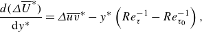 \begin{align} &\qquad\qquad\frac {d (\unicode{x1D6E5} \overline {U}^*)}{{\mathrm d}y^*} = \unicode{x1D6E5} \overline { u v }^* - y^*\left ( {Re_\tau ^{-1}} - {Re_{\tau _0}^{-1}} \right ), \end{align}
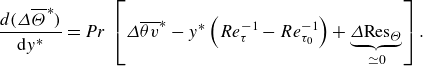 \begin{align} &\frac {d(\unicode{x1D6E5} \overline {\Theta }^*)}{{\mathrm d}y^*} = Pr \, \left [ \unicode{x1D6E5} \overline { \theta v }^* - y^*\left ( {Re_\tau ^{-1}} - {Re_{\tau _0}^{-1}} \right ) + \underbrace {\unicode{x1D6E5} \mbox{Res}_{\Theta }}_{\simeq 0} \right ]. \end{align}
The difference $\unicode{x1D6E5} \mbox{Res}_{\Theta }$
between the actuated and non-actuated cases is small and can be neglected. The remaining terms in (3.3a
) and (3.3b
) are plotted in figure 10 for the travelling wave case at
$\unicode{x1D6E5} \mbox{Res}_{\Theta }$
between the actuated and non-actuated cases is small and can be neglected. The remaining terms in (3.3a
) and (3.3b
) are plotted in figure 10 for the travelling wave case at $Pr = 7.5$
and
$Pr = 7.5$
and $\omega ^+=0.088$
. We see that the right-hand-side of (3.3a
) and (3.3b
) are dominated by
$\omega ^+=0.088$
. We see that the right-hand-side of (3.3a
) and (3.3b
) are dominated by $\unicode{x1D6E5} \overline {uv}^*$
and
$\unicode{x1D6E5} \overline {uv}^*$
and $\unicode{x1D6E5} \overline {\theta v}^*$
, up to their respective minima, but farther from the wall these terms are cancelled by the term containing the difference in Reynolds numbers
$\unicode{x1D6E5} \overline {\theta v}^*$
, up to their respective minima, but farther from the wall these terms are cancelled by the term containing the difference in Reynolds numbers $ ( {Re_\tau ^{-1}} - {Re_{\tau _0}^{-1}} )$
. That is, the net contributions to
$ ( {Re_\tau ^{-1}} - {Re_{\tau _0}^{-1}} )$
. That is, the net contributions to $\unicode{x1D6E5} \overline {U}^*$
and
$\unicode{x1D6E5} \overline {U}^*$
and $\unicode{x1D6E5} \overline {\Theta }^*$
, hence, DR and HR, come from
$\unicode{x1D6E5} \overline {\Theta }^*$
, hence, DR and HR, come from $\unicode{x1D6E5} \overline {uv}^*$
and
$\unicode{x1D6E5} \overline {uv}^*$
and $\unicode{x1D6E5} \overline {\theta v}^*$
, and then only up to the points where
$\unicode{x1D6E5} \overline {\theta v}^*$
, and then only up to the points where $\unicode{x1D6E5} \overline {uv}^*$
and
$\unicode{x1D6E5} \overline {uv}^*$
and $\unicode{x1D6E5} \overline {\theta v}^*$
reach their minimum values.
$\unicode{x1D6E5} \overline {\theta v}^*$
reach their minimum values.
3.4.
Source of inequality between
$HR$
and
$DR$


Integrating (3.3a
) and (3.3b
) once more with respect to $y^*$
gives
$y^*$
gives
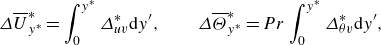 \begin{align} \unicode{x1D6E5} \overline {U}^*_{y^*} =\int _0^{y^*} \unicode{x1D6E5} ^*_{uv} {\mathrm d}y', \qquad \unicode{x1D6E5} \overline {\Theta }^*_{y^*} = Pr \int _0^{y^*} \unicode{x1D6E5} ^*_{\theta v} {\mathrm d}y', \end{align}
where
 \begin{align} \unicode{x1D6E5} ^*_{uv} \equiv \unicode{x1D6E5} \overline { u v }^* - y^*(Re_\tau ^{-1} - Re_{\tau _0}^{-1}), \end{align}
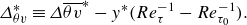 \begin{align} \unicode{x1D6E5} ^*_{\theta v} \equiv \unicode{x1D6E5} \overline { \theta v }^* - y^*(Re_\tau ^{-1} - Re_{\tau _0}^{-1}). \end{align}
By using (3.4a
) we can relate $\unicode{x1D6E5} ^*_{uv}$
and
$\unicode{x1D6E5} ^*_{uv}$
and $\unicode{x1D6E5} ^*_{\theta v}$
to
$\unicode{x1D6E5} ^*_{\theta v}$
to $\unicode{x1D6E5} \overline {U}^*$
and
$\unicode{x1D6E5} \overline {U}^*$
and $\unicode{x1D6E5} \overline {\Theta }^*$
, hence, to DR and HR, and so establish the connection between the DR and HR and the turbulence attenuation. For the DR, Gatti & Quadrio (Reference Gatti and Quadrio2016) derived the relation between DR (
$\unicode{x1D6E5} \overline {\Theta }^*$
, hence, to DR and HR, and so establish the connection between the DR and HR and the turbulence attenuation. For the DR, Gatti & Quadrio (Reference Gatti and Quadrio2016) derived the relation between DR ( $=1-R_f$
) and the asymptotic value of
$=1-R_f$
) and the asymptotic value of $\unicode{x1D6E5} \overline {U}^*$
in the log region (3.5a
). In Appendix B we derive a similar relation between HR (
$\unicode{x1D6E5} \overline {U}^*$
in the log region (3.5a
). In Appendix B we derive a similar relation between HR ( $=1-R_h$
) and the asymptotic value of
$=1-R_h$
) and the asymptotic value of $\unicode{x1D6E5} \overline {\Theta }^*$
in the log region (3.5b
). That is, we have
$\unicode{x1D6E5} \overline {\Theta }^*$
in the log region (3.5b
). That is, we have
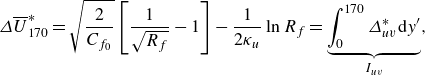 \begin{align} &\quad\unicode{x1D6E5} \overline {U}^*_{170} = \sqrt {\frac {2}{C_{{f_0}}}}\left [ \frac {1}{\sqrt {R_f}} - 1 \right ] - \frac {1}{2\kappa _u}\ln {R_f} = \underbrace {\int ^{170}_0 \unicode{x1D6E5} ^*_{uv} {\mathrm d}y'}_{I_{uv}}, \end{align}
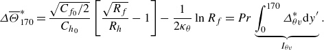 \begin{align} &\unicode{x1D6E5} \overline {\Theta }^*_{170} = \frac {\sqrt {C_{{f_0}}/2}}{C_{{h_0}}}\left [ \frac {\sqrt {R_f}}{R_h} - 1 \right ] - \frac {1}{2\kappa _\theta }\ln {R_f} = Pr \underbrace {\int ^{170}_0 \unicode{x1D6E5} ^*_{\theta v} {\mathrm d}y'}_{I_{\theta v}}. \end{align}
These derivations assume that the profiles of $\overline {U}^*$
and
$\overline {U}^*$
and $\overline {\Theta }^*$
have well-defined log regions with slopes that are not affected by the wall oscillation, which is the case for our results (figure 8). The integration was performed up to
$\overline {\Theta }^*$
have well-defined log regions with slopes that are not affected by the wall oscillation, which is the case for our results (figure 8). The integration was performed up to $y^*_{{res}} = 170$
, where the profiles of
$y^*_{{res}} = 170$
, where the profiles of $\unicode{x1D6E5} \overline {U}^*$
and
$\unicode{x1D6E5} \overline {U}^*$
and $\unicode{x1D6E5} \overline {\Theta }^*$
reach their asymptotic levels (figure 8
j,k,l) and their derivatives are zero (figure 10). On the right-hand sides of (3.5a
) and (3.5b
) we have the integrals of attenuation in the turbulent shear stress (
$\unicode{x1D6E5} \overline {\Theta }^*$
reach their asymptotic levels (figure 8
j,k,l) and their derivatives are zero (figure 10). On the right-hand sides of (3.5a
) and (3.5b
) we have the integrals of attenuation in the turbulent shear stress ( $I_{uv}$
) and the turbulent temperature flux (
$I_{uv}$
) and the turbulent temperature flux ( $I_{\theta v}$
). For a fixed set of viscous-scaled actuation parameters,
$I_{\theta v}$
). For a fixed set of viscous-scaled actuation parameters, $I_{uv} = \unicode{x1D6E5} \overline {U}^*_{170}$
is constant (Gatti & Quadrio Reference Gatti and Quadrio2016; Rouhi et al. Reference Rouhi, Fu, Chandran, Zampiron, Smits and Marusic2023) (also shown in figure 8
j), but
$I_{uv} = \unicode{x1D6E5} \overline {U}^*_{170}$
is constant (Gatti & Quadrio Reference Gatti and Quadrio2016; Rouhi et al. Reference Rouhi, Fu, Chandran, Zampiron, Smits and Marusic2023) (also shown in figure 8
j), but $I_{\theta v} = \unicode{x1D6E5} \overline {\Theta }^*_{170}/Pr$
depends on
$I_{\theta v} = \unicode{x1D6E5} \overline {\Theta }^*_{170}/Pr$
depends on $Pr$
(figure 9
k,l).
$Pr$
(figure 9
k,l).
To predict DR and HR from (3.5a
) and (3.5b
), we only need $\unicode{x1D6E5} \overline {U}^*_{170}$
and
$\unicode{x1D6E5} \overline {U}^*_{170}$
and $\unicode{x1D6E5} \overline {\Theta }^*_{170}$
(that is,
$\unicode{x1D6E5} \overline {\Theta }^*_{170}$
(that is, $I_{uv}$
and
$I_{uv}$
and $I_{\theta v}$
) as the inputs; the other parameters are associated with the non-actuated channel flow for which semi-empirical relations exist in the literature. We choose
$I_{\theta v}$
) as the inputs; the other parameters are associated with the non-actuated channel flow for which semi-empirical relations exist in the literature. We choose $\kappa _u = 0.4$
and
$\kappa _u = 0.4$
and $\kappa _\theta = 0.46$
(Pirozzoli et al. Reference Pirozzoli, Bernardini and Orlandi2016); the suitability of these choices is confirmed in § 2.3 and Appendix A. Dean (Reference Dean1978)’s correlation is used for the non-actuated skin-friction coefficient
$\kappa _\theta = 0.46$
(Pirozzoli et al. Reference Pirozzoli, Bernardini and Orlandi2016); the suitability of these choices is confirmed in § 2.3 and Appendix A. Dean (Reference Dean1978)’s correlation is used for the non-actuated skin-friction coefficient $C_{f_0} = 0.073(2Re_b)^{-1/4}$
, which could be re-expressed as
$C_{f_0} = 0.073(2Re_b)^{-1/4}$
, which could be re-expressed as $C_{{f_0}} = 0.037Re^{-2/7}_{\tau _0}$
; this correlation agrees well with the DNS data (MacDonald et al. Reference MacDonald, Hutchins and Chung2019), and yields less than
$C_{{f_0}} = 0.037Re^{-2/7}_{\tau _0}$
; this correlation agrees well with the DNS data (MacDonald et al. Reference MacDonald, Hutchins and Chung2019), and yields less than $2\,\%$
difference with our DNS result
$2\,\%$
difference with our DNS result $C_{f_0} = 0.0057$
at
$C_{f_0} = 0.0057$
at $Re_{\tau _0} = 590$
. For the non-actuated
$Re_{\tau _0} = 590$
. For the non-actuated $C_{h_0}$
, in figure 11 we compare our DNS data at
$C_{h_0}$
, in figure 11 we compare our DNS data at $Re_{\tau _0} = 590$
and different
$Re_{\tau _0} = 590$
and different $Pr$
(cases on the left side of table 1) with several empirical relations. These relations define
$Pr$
(cases on the left side of table 1) with several empirical relations. These relations define $C_{h_0}$
either based on the bulk temperature
$C_{h_0}$
either based on the bulk temperature $\Theta _b$
or the mixed-mean temperature
$\Theta _b$
or the mixed-mean temperature $\Theta _m$
. For our DNS data, there is a negligible difference between the two definitions (empty versus the filled circles). Among the relations, the latest correlation by Pirozzoli et al. (Reference Pirozzoli, Romero, Fatica, Verzicco and Orlandi2022) agrees well with our DNS data (solid black line). This relation is an improvement to Kader & Yaglom (Reference Kader and Yaglom1972)’s formula, and its accuracy is supported by the recent DNS of Pirozzoli (Reference Pirozzoli2023) for
$\Theta _m$
. For our DNS data, there is a negligible difference between the two definitions (empty versus the filled circles). Among the relations, the latest correlation by Pirozzoli et al. (Reference Pirozzoli, Romero, Fatica, Verzicco and Orlandi2022) agrees well with our DNS data (solid black line). This relation is an improvement to Kader & Yaglom (Reference Kader and Yaglom1972)’s formula, and its accuracy is supported by the recent DNS of Pirozzoli (Reference Pirozzoli2023) for $\mathcal{O}(10^{-2}) \lesssim Pr \lesssim \mathcal{O}(10^{1})$
. It is formulated as
$\mathcal{O}(10^{-2}) \lesssim Pr \lesssim \mathcal{O}(10^{1})$
. It is formulated as
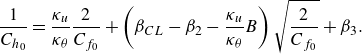 \begin{align} \frac {1}{C_{{h_0}}} = \frac {\kappa _u}{\kappa _\theta }\frac {2}{C_{{f_0}}} + \left ( \beta _{CL} - \beta _2 - \frac {\kappa _u}{\kappa _\theta }B \right )\sqrt {\frac {2}{C_{{f_0}}}} + \beta _3. \end{align}
Here $\beta _{CL}(Pr) = B_\theta (Pr) + 3.504 - 1.5/\kappa _\theta$
,
$\beta _{CL}(Pr) = B_\theta (Pr) + 3.504 - 1.5/\kappa _\theta$
, $\beta _2 = 4.92$
,
$\beta _2 = 4.92$
, $\beta _3 = 39.6$
,
$\beta _3 = 39.6$
, $B = 1.23$
and
$B = 1.23$
and $B_\theta (Pr)$
is the log-law additive constant for
$B_\theta (Pr)$
is the log-law additive constant for $\overline {\Theta }^*$
(Kader & Yaglom Reference Kader and Yaglom1972), as introduced in Appendix B.
$\overline {\Theta }^*$
(Kader & Yaglom Reference Kader and Yaglom1972), as introduced in Appendix B.
Comparison of the non-actuated $C_{h_0}$
between our DNS cases (left side of table 1) and several empirical relations. For the DNS data,
$C_{h_0}$
between our DNS cases (left side of table 1) and several empirical relations. For the DNS data, $C_{h_0}$
is calculated either based on the bulk temperature
$C_{h_0}$
is calculated either based on the bulk temperature $\Theta _b$
(empty symbols) or the mixed-mean temperature
$\Theta _b$
(empty symbols) or the mixed-mean temperature $\Theta _m$
(filled symbols). The empirical relations are by Pirozzoli et al. (Reference Pirozzoli, Romero, Fatica, Verzicco and Orlandi2022) (3.6), Kays et al. (Reference Kays, Crawford and Weigand1993), Kader & Yaglom (Reference Kader and Yaglom1972), Kakaç et al. (Reference Kakaç, Shah and Aung1987), Chilton--Colburn analogy (Chilton & Colburn Reference Chilton and Colburn1934; Colburn Reference Colburn1964), Prandtl analogy (see equation 11 in Schlünder Reference Schlünder1998) and the von Kármán analogy (see equation 4 in Li & Li Reference Li and Li2010).
$\Theta _m$
(filled symbols). The empirical relations are by Pirozzoli et al. (Reference Pirozzoli, Romero, Fatica, Verzicco and Orlandi2022) (3.6), Kays et al. (Reference Kays, Crawford and Weigand1993), Kader & Yaglom (Reference Kader and Yaglom1972), Kakaç et al. (Reference Kakaç, Shah and Aung1987), Chilton--Colburn analogy (Chilton & Colburn Reference Chilton and Colburn1934; Colburn Reference Colburn1964), Prandtl analogy (see equation 11 in Schlünder Reference Schlünder1998) and the von Kármán analogy (see equation 4 in Li & Li Reference Li and Li2010).
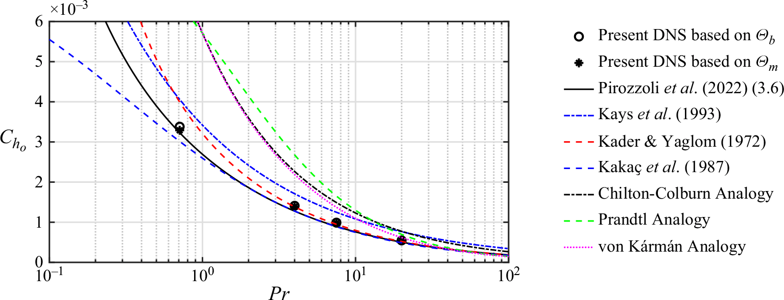
Travelling wave actuation with $A^+ = 12$
,
$A^+ = 12$
, $\kappa ^+_x = 0.0014$
. Comparison between the direct HR from DNS (filled squares) and the predicted HR (empty triangles) by solving (3.5a
) and (3.5b
). In (a), for predicting HR, we use
$\kappa ^+_x = 0.0014$
. Comparison between the direct HR from DNS (filled squares) and the predicted HR (empty triangles) by solving (3.5a
) and (3.5b
). In (a), for predicting HR, we use $I_{uv}$
and
$I_{uv}$
and $I_{\theta v}$
directly from DNS. In (b), for predicting HR, we use a power-law estimate for
$I_{\theta v}$
directly from DNS. In (b), for predicting HR, we use a power-law estimate for $I_{\theta v} = I_{uv}/Pr^\gamma$
, with the values of
$I_{\theta v} = I_{uv}/Pr^\gamma$
, with the values of $\gamma$
reported in figure 13(b).
$\gamma$
reported in figure 13(b).
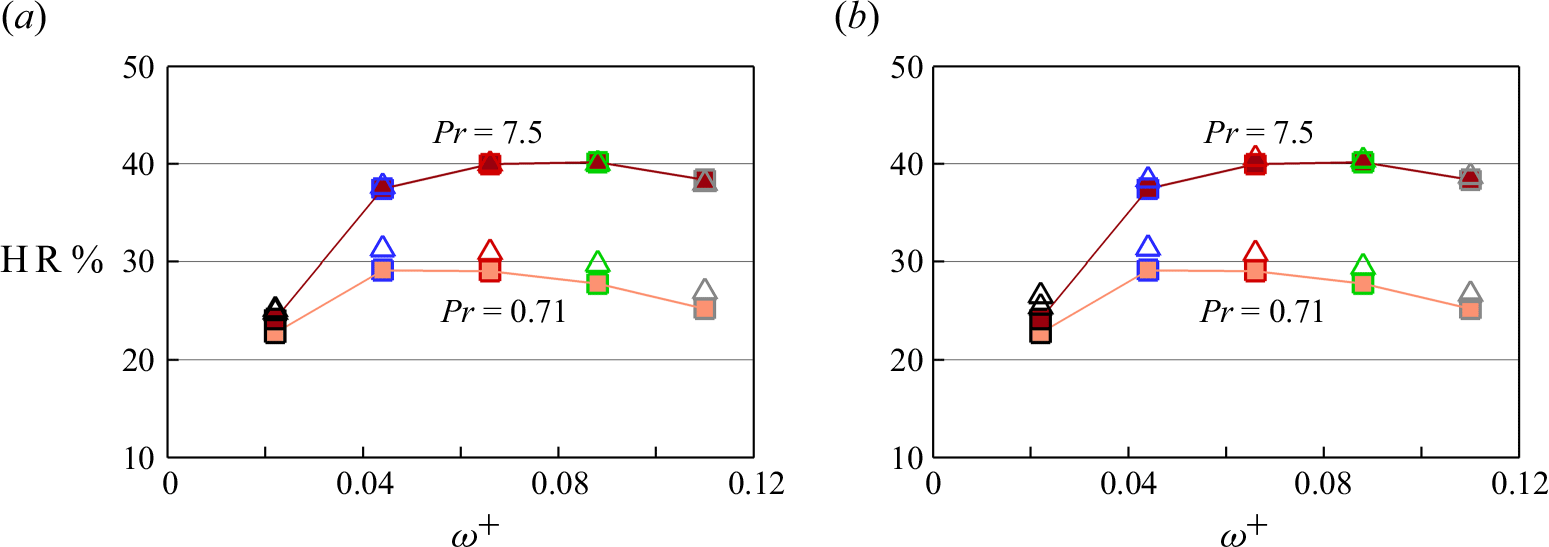
Travelling wave at $Pr = 0.71, 4.0$
and
$Pr = 0.71, 4.0$
and $7.5$
(same data as in figure 5
a,c,e). The outline colour of each data point indicates its
$7.5$
(same data as in figure 5
a,c,e). The outline colour of each data point indicates its $\omega ^+$
;
$\omega ^+$
; $\omega ^+ = 0.022$
(black),
$\omega ^+ = 0.022$
(black), $0.044$
(blue),
$0.044$
(blue), $0.066$
(red),
$0.066$
(red), $0.088$
(green) and
$0.088$
(green) and $0.110$
(grey). (a) Plot of
$0.110$
(grey). (a) Plot of $I_{\theta v}$
versus
$I_{\theta v}$
versus $I_{uv}$
; the dotted line is for
$I_{uv}$
; the dotted line is for $I_{\theta v}=I_{uv}$
. (b) Plot of
$I_{\theta v}=I_{uv}$
. (b) Plot of $I_{\theta v}$
versus
$I_{\theta v}$
versus $Pr$
; the solid curves are the power-law fit
$Pr$
; the solid curves are the power-law fit $I_{\theta v} = I_{u v}/Pr^{\gamma }$
, with
$I_{\theta v} = I_{u v}/Pr^{\gamma }$
, with $\gamma$
as shown. (c,d) Plots of HR and
$\gamma$
as shown. (c,d) Plots of HR and ${\textrm{HR}}-{\textrm{DR}}$
versus
${\textrm{HR}}-{\textrm{DR}}$
versus $Pr$
; the solid curves are the prediction of (3.5b
) using
$Pr$
; the solid curves are the prediction of (3.5b
) using $I_{\theta v} = I_{u v}/Pr^{\gamma }$
. In (d), the blue zone marks
$I_{\theta v} = I_{u v}/Pr^{\gamma }$
. In (d), the blue zone marks $\gamma \gt 0.5$
and the grey zone marks
$\gamma \gt 0.5$
and the grey zone marks $\gamma \lt 0.5$
.
$\gamma \lt 0.5$
.
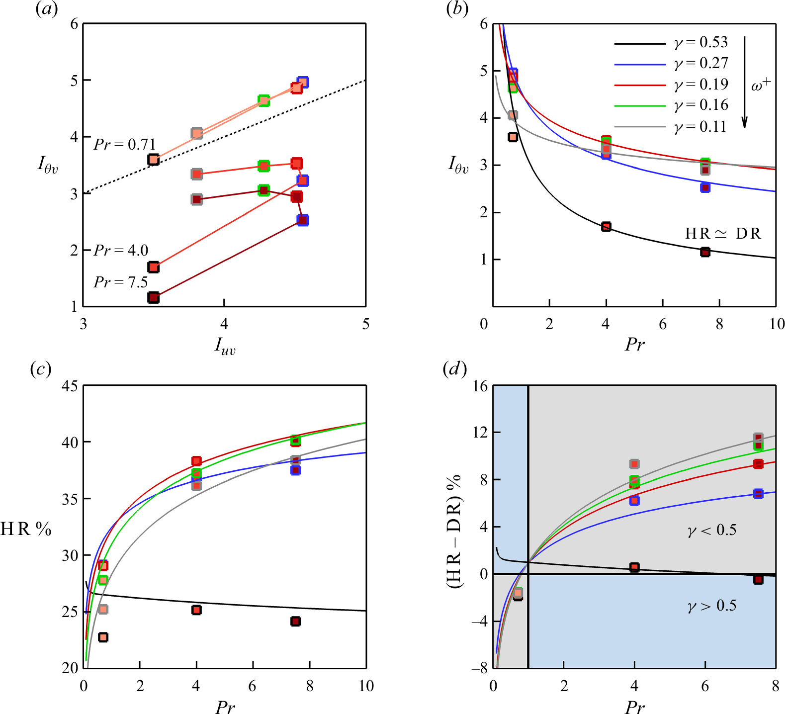
In figure 12(a) we compare the values of HR from DNS with those from (3.5a
) and (3.5b
) using $I_{uv}$
and
$I_{uv}$
and $I_{\theta v}$
as obtained from DNS. The results support the accuracy of the model for relating HR to the attenuation of the turbulent flux. In figure 12(b) we also show the agreement between the model and the DNS when we use a power-law estimate for
$I_{\theta v}$
as obtained from DNS. The results support the accuracy of the model for relating HR to the attenuation of the turbulent flux. In figure 12(b) we also show the agreement between the model and the DNS when we use a power-law estimate for $I_{\theta v}$
(
$I_{\theta v}$
( $=I_{uv}/Pr^{\gamma }$
) where only
$=I_{uv}/Pr^{\gamma }$
) where only $I_{uv}$
(which is independent of
$I_{uv}$
(which is independent of $Pr$
) is obtained from DNS. We justify the power law as follows.
$Pr$
) is obtained from DNS. We justify the power law as follows.
From (3.5b
), we note that the Prandtl number dependence of HR (hence ${\textrm{HR}}- {\textrm{DR}}$
) is due to both
${\textrm{HR}}- {\textrm{DR}}$
) is due to both $C_{{h_0}}$
and
$C_{{h_0}}$
and $ I_{\theta v}$
. According to the Reynolds analogy, we would expect
$ I_{\theta v}$
. According to the Reynolds analogy, we would expect $I_{\theta v} = I_{u v}$
when
$I_{\theta v} = I_{u v}$
when $Pr = 1.0$
. Figure 13(a) indicates that, regardless of the actuation frequency
$Pr = 1.0$
. Figure 13(a) indicates that, regardless of the actuation frequency $\omega ^+$
,
$\omega ^+$
, $I_{\theta v} \gt I_{u v}$
for
$I_{\theta v} \gt I_{u v}$
for $Pr = 0.71$
and
$Pr = 0.71$
and $I_{\theta v} \lt I_{u v}$
for
$I_{\theta v} \lt I_{u v}$
for $Pr \gt 1$
, with the difference increasing with
$Pr \gt 1$
, with the difference increasing with $Pr$
. In other words, increasing
$Pr$
. In other words, increasing $Pr$
beyond unity leads to a lower attenuation of
$Pr$
beyond unity leads to a lower attenuation of $\overline {\theta v}$
compared with
$\overline {\theta v}$
compared with $\overline {u v}$
, even though in this regime
$\overline {u v}$
, even though in this regime ${\textrm{HR}} \gt {\textrm{DR}}$
(figure 5
c–f). Figure 13(b) shows how
${\textrm{HR}} \gt {\textrm{DR}}$
(figure 5
c–f). Figure 13(b) shows how $I_{\theta v}$
depends on
$I_{\theta v}$
depends on $Pr$
, and that
$Pr$
, and that $I_{\theta v} = I_{uv}/Pr^\gamma$
is a good approximation to the data. For the present data with a fixed
$I_{\theta v} = I_{uv}/Pr^\gamma$
is a good approximation to the data. For the present data with a fixed $A^+$
and
$A^+$
and $\kappa ^+_x$
,
$\kappa ^+_x$
, $\gamma$
depends on
$\gamma$
depends on $\omega ^+$
but it is independent of
$\omega ^+$
but it is independent of $Pr$
. When we use this power law in (3.5b) and solve for HR by using
$Pr$
. When we use this power law in (3.5b) and solve for HR by using $I_{uv}$
from DNS, figure 13(c,d) shows that the model closely matches the data. Furthermore, for
$I_{uv}$
from DNS, figure 13(c,d) shows that the model closely matches the data. Furthermore, for $\gamma \lt 0.5$
, we can achieve
$\gamma \lt 0.5$
, we can achieve ${\textrm{HR}} \gt {\textrm{DR}}$
for
${\textrm{HR}} \gt {\textrm{DR}}$
for $Pr \gt 1$
, and the smaller
$Pr \gt 1$
, and the smaller $\gamma$
is the higher HR compared with DR. From figure 13(b,d), as
$\gamma$
is the higher HR compared with DR. From figure 13(b,d), as $\omega ^+$
increases from
$\omega ^+$
increases from $0.022$
(black curve) to
$0.022$
(black curve) to $0.110$
(grey curve),
$0.110$
(grey curve), $\gamma$
decreases from approximately
$\gamma$
decreases from approximately $0.5$
to
$0.5$
to $0.1$
, and
$0.1$
, and ${\textrm{HR}}-{\textrm{DR}}$
increases from almost zero to
${\textrm{HR}}-{\textrm{DR}}$
increases from almost zero to $10\,\%$
. Therefore, we expect
$10\,\%$
. Therefore, we expect ${\textrm{HR}}\lt {\textrm{DR}}$
for
${\textrm{HR}}\lt {\textrm{DR}}$
for $Pr \gt 1.0$
if
$Pr \gt 1.0$
if $\gamma \gt 0.5$
. This occurs for the plane oscillation at
$\gamma \gt 0.5$
. This occurs for the plane oscillation at $\omega ^+ = 0.022$
, where
$\omega ^+ = 0.022$
, where $\gamma = 2.43$
and
$\gamma = 2.43$
and ${\textrm{HR}}- {\textrm{DR}} \simeq -5\,\%$
(figure 21).
${\textrm{HR}}- {\textrm{DR}} \simeq -5\,\%$
(figure 21).
Predicted maps of (a,c) HR and (b,d) ${\textrm{HR}}-{\textrm{DR}}$
for the travelling wave with
${\textrm{HR}}-{\textrm{DR}}$
for the travelling wave with $A^+ = 12, \kappa ^+_x = 0.0014$
and
$A^+ = 12, \kappa ^+_x = 0.0014$
and $\omega ^+ = 0.088$
. Plots (a,b) are obtained from our proposed model
$\omega ^+ = 0.088$
. Plots (a,b) are obtained from our proposed model $I_{\theta v} = I_{uv}/Pr^{\gamma }$
with
$I_{\theta v} = I_{uv}/Pr^{\gamma }$
with $I_{uv} = 4.28, \gamma = 0.16$
obtained from DNS, and by solving (3.5
a
, 3.5b
).Plots (c,d) are obtained from the simplified model (3.7a
, 3.7b
) and by solving (3.5a
, 3.5b
). The white bullets represent DNS results at
$I_{uv} = 4.28, \gamma = 0.16$
obtained from DNS, and by solving (3.5
a
, 3.5b
).Plots (c,d) are obtained from the simplified model (3.7a
, 3.7b
) and by solving (3.5a
, 3.5b
). The white bullets represent DNS results at $Re_{\tau _0} = 590$
for
$Re_{\tau _0} = 590$
for $Pr = 0.71, 4.0, 7.5$
and
$Pr = 0.71, 4.0, 7.5$
and $20$
.
$20$
.
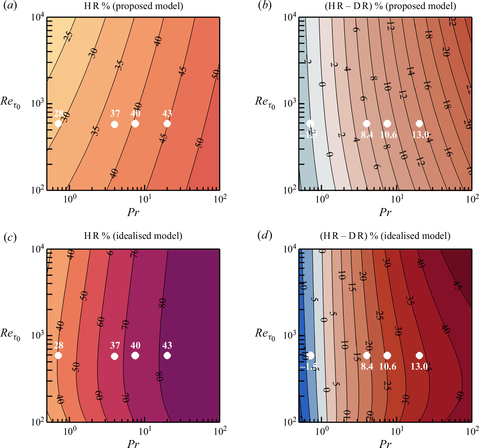
3.5. Heat-transfer reduction at higher Prandtl number and Reynolds number
Gatti & Quadrio (Reference Gatti and Quadrio2016) used (3.5a
) to extrapolate their low-Reynolds-number DR data to higher Reynolds numbers, and the accuracy of this extrapolation was corroborated by Rouhi et al. (Reference Rouhi, Fu, Chandran, Zampiron, Smits and Marusic2023) up to $Re_{\tau _0} = 4000$
using LES and by Gatti et al. (Reference Gatti, Quadrio, Chiarini, Gattere and Pirozzoli2024) up to
$Re_{\tau _0} = 4000$
using LES and by Gatti et al. (Reference Gatti, Quadrio, Chiarini, Gattere and Pirozzoli2024) up to $Re_{\tau _0} = 6000$
using DNS. For a fixed set of actuation parameters
$Re_{\tau _0} = 6000$
using DNS. For a fixed set of actuation parameters $(A^+,\kappa ^+_x,\omega ^+)$
,
$(A^+,\kappa ^+_x,\omega ^+)$
, $I_{uv}$
is Reynolds and Prandtl number independent, and so the only Reynolds number dependency of DR is through
$I_{uv}$
is Reynolds and Prandtl number independent, and so the only Reynolds number dependency of DR is through $C_{f_0}$
. Hence, Gatti & Quadrio (Reference Gatti and Quadrio2016) could solve (3.5a
) and predict DR at any Reynolds number. We can now do the same for HR by using the power-law relationship
$C_{f_0}$
. Hence, Gatti & Quadrio (Reference Gatti and Quadrio2016) could solve (3.5a
) and predict DR at any Reynolds number. We can now do the same for HR by using the power-law relationship $I_{\theta v} = I_{uv}/Pr^{\gamma }$
. By knowing
$I_{\theta v} = I_{uv}/Pr^{\gamma }$
. By knowing $I_{uv}$
and
$I_{uv}$
and $\gamma$
for a fixed set of actuation parameters, we can then solve (3.5a
) and (3.5b
) to map HR and
$\gamma$
for a fixed set of actuation parameters, we can then solve (3.5a
) and (3.5b
) to map HR and ${\textrm{HR}}- {\textrm{DR}}$
as functions of
${\textrm{HR}}- {\textrm{DR}}$
as functions of $Pr$
and
$Pr$
and $Re_{\tau _0}$
.
$Re_{\tau _0}$
.
Characteristics of the Stokes layer for the travelling wave with $A^+ = 12, \kappa ^+_x = 0.0014$
and
$A^+ = 12, \kappa ^+_x = 0.0014$
and $0.022 \le \omega ^+ \le 0.110$
(same cases as in figure 5
a,c,e). Results are independent of Prandtl number. The colour of the profiles and data points change from black at
$0.022 \le \omega ^+ \le 0.110$
(same cases as in figure 5
a,c,e). Results are independent of Prandtl number. The colour of the profiles and data points change from black at $\omega ^+ = 0.022$
to light grey at
$\omega ^+ = 0.022$
to light grey at $\omega ^+ = 0.110$
. (a) Profiles of
$\omega ^+ = 0.110$
. (a) Profiles of $\overline { \tilde {w}^2 }^*$
. Stokes layer protrusion height
$\overline { \tilde {w}^2 }^*$
. Stokes layer protrusion height $\ell ^*_{0.01}$
(Rouhi et al. Reference Rouhi, Fu, Chandran, Zampiron, Smits and Marusic2023) marked at
$\ell ^*_{0.01}$
(Rouhi et al. Reference Rouhi, Fu, Chandran, Zampiron, Smits and Marusic2023) marked at $\overline { \tilde {w}^2}^* = 0.01$
(filled bullets); laminar Stokes layer thickness
$\overline { \tilde {w}^2}^* = 0.01$
(filled bullets); laminar Stokes layer thickness $\delta ^*_S$
marked at
$\delta ^*_S$
marked at $\overline { \tilde {w}^2}^* = ({1}/{2}){A^*}^2\textrm{e}^{-2}$
(cross symbols). (b) Production due to the Stokes layer
$\overline { \tilde {w}^2}^* = ({1}/{2}){A^*}^2\textrm{e}^{-2}$
(cross symbols). (b) Production due to the Stokes layer $P^*_{33}$
. (c)Plot of
$P^*_{33}$
. (c)Plot of $\ell ^*_{0.01}$
(filled bullets) and
$\ell ^*_{0.01}$
(filled bullets) and $\delta ^*_S$
(cross symbols) versus the maximum value of
$\delta ^*_S$
(cross symbols) versus the maximum value of $\tilde {P}^*_{33}$
.
$\tilde {P}^*_{33}$
.

In figure 14(a,b) we show these predictions for the travelling wave case with $\omega ^+ = 0.088$
, where the DNS gives
$\omega ^+ = 0.088$
, where the DNS gives $I_{uv} = 4.28$
and
$I_{uv} = 4.28$
and $\gamma = 0.16$
(data points with green outline in figure 13). The predictions agree well with the DNS data points, including the point at
$\gamma = 0.16$
(data points with green outline in figure 13). The predictions agree well with the DNS data points, including the point at $Pr = 20$
(
$Pr = 20$
( ${\textrm{HR}} = 43\,\%, {\textrm{HR}} - {\textrm{DR}} = 13\,\%$
) (see table 1). At a given Reynolds number, HR increases almost logarithmically with Prandtl number. For instance, at
${\textrm{HR}} = 43\,\%, {\textrm{HR}} - {\textrm{DR}} = 13\,\%$
) (see table 1). At a given Reynolds number, HR increases almost logarithmically with Prandtl number. For instance, at $Re_{\tau _0} = 590$
HR increases from
$Re_{\tau _0} = 590$
HR increases from $30\,\%$
to
$30\,\%$
to $40\,\%$
as the Prandtl number increases from 0.71 to 7.5, and
$40\,\%$
as the Prandtl number increases from 0.71 to 7.5, and ${\textrm{HR}} = 50\,\%$
would be obtained at a Prandtl number of approximately 75. In addition, HR decreases very slowly with increasing
${\textrm{HR}} = 50\,\%$
would be obtained at a Prandtl number of approximately 75. In addition, HR decreases very slowly with increasing $Re_{\tau _0}$
. For instance, at
$Re_{\tau _0}$
. For instance, at $Pr = 7.5$
HR decreases from
$Pr = 7.5$
HR decreases from $40\,\%$
to approximately
$40\,\%$
to approximately $36\,\%$
as
$36\,\%$
as $Re_{\tau _0}$
increases from
$Re_{\tau _0}$
increases from $590$
to
$590$
to $5900$
. Such a slow decrease with
$5900$
. Such a slow decrease with $Re_{\tau _0}$
is similarly observed in the predictive model for DR (3.5a
) (Marusic et al. Reference Marusic, Chandran, Rouhi, Fu, Wine, Holloway, Chung and Smits2021; Rouhi et al. Reference Rouhi, Fu, Chandran, Zampiron, Smits and Marusic2023; Gatti et al. Reference Gatti, Quadrio, Chiarini, Gattere and Pirozzoli2024).
$Re_{\tau _0}$
is similarly observed in the predictive model for DR (3.5a
) (Marusic et al. Reference Marusic, Chandran, Rouhi, Fu, Wine, Holloway, Chung and Smits2021; Rouhi et al. Reference Rouhi, Fu, Chandran, Zampiron, Smits and Marusic2023; Gatti et al. Reference Gatti, Quadrio, Chiarini, Gattere and Pirozzoli2024).
In figure 14(c,d) we predict HR and ${\textrm{HR}}-{\textrm{DR}}$
for the same actuated case as in figure 14(a,b), but with a simplified analytical approach, similar to that proposed by Iwamoto et al. (Reference Iwamoto, Fukagata, Kasagi and Suzuki2005). The approach assumes that turbulence is completely damped in the near-wall region, which here we consider that to be up to the Stokes layer protrusion height
${\textrm{HR}}-{\textrm{DR}}$
for the same actuated case as in figure 14(a,b), but with a simplified analytical approach, similar to that proposed by Iwamoto et al. (Reference Iwamoto, Fukagata, Kasagi and Suzuki2005). The approach assumes that turbulence is completely damped in the near-wall region, which here we consider that to be up to the Stokes layer protrusion height $\ell ^*_{0.01}$
(figure 15
a). Therefore, for
$\ell ^*_{0.01}$
(figure 15
a). Therefore, for $0 \le y^* \le \ell ^*_{0.01}$
, the profiles are assumed to be laminar
$0 \le y^* \le \ell ^*_{0.01}$
, the profiles are assumed to be laminar $\overline {U}^* = y^*[1-y^*/(2Re_\tau )], \overline {\Theta }^* = Pr y^*[1-y^*/(2Re_\tau )]$
, and for
$\overline {U}^* = y^*[1-y^*/(2Re_\tau )], \overline {\Theta }^* = Pr y^*[1-y^*/(2Re_\tau )]$
, and for $y^* \gt \ell ^*_{0.01}$
, the profiles follow the turbulent formulations (C1a
,) (C1b
). By matching the laminar and turbulent profiles at
$y^* \gt \ell ^*_{0.01}$
, the profiles follow the turbulent formulations (C1a
,) (C1b
). By matching the laminar and turbulent profiles at $y^* = \ell ^*_{0.01}$
, we obtain
$y^* = \ell ^*_{0.01}$
, we obtain
 \begin{align} &\,\,\,\,\unicode{x1D6E5} \overline {U}^*_{170} = \ell ^*_{0.01} \left ( 1 - \frac {\ell ^*_{0.01}}{ 2Re_\tau } \right ) - \left ( \frac {1}{\kappa _u}\ln \ell ^*_{0.01} + B_u \right ), \end{align}
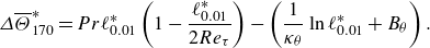 \begin{align} &\unicode{x1D6E5} \overline {\Theta }^*_{170} = Pr \ell ^*_{0.01} \left ( 1 - \frac {\ell ^*_{0.01}}{ 2Re_\tau } \right ) - \left ( \frac {1}{\kappa _\theta }\ln \ell ^*_{0.01} + B_\theta \right ). \end{align}
We substitute for $\unicode{x1D6E5} \overline {U}^*_{170}, \unicode{x1D6E5} \overline {\Theta }^*_{170}$
in (3.5a
), (3.5b
) to predict HR and
$\unicode{x1D6E5} \overline {U}^*_{170}, \unicode{x1D6E5} \overline {\Theta }^*_{170}$
in (3.5a
), (3.5b
) to predict HR and ${\textrm{HR}}-{\textrm{DR}}$
. With this approach, the predicted HR and
${\textrm{HR}}-{\textrm{DR}}$
. With this approach, the predicted HR and ${\textrm{HR}}-{\textrm{DR}}$
increase with
${\textrm{HR}}-{\textrm{DR}}$
increase with $Pr$
(figure 14
c,d), consistent with our proposed model and DNS (figure 14
a,b). However, quantitatively, this approach overpredicts HR and
$Pr$
(figure 14
c,d), consistent with our proposed model and DNS (figure 14
a,b). However, quantitatively, this approach overpredicts HR and ${\textrm{HR}}-{\textrm{DR}}$
by two times compared with the DNS data and our proposed model, which is of no surprise. The Stokes layer does not completely attenuate the near-wall turbulence, even down to
${\textrm{HR}}-{\textrm{DR}}$
by two times compared with the DNS data and our proposed model, which is of no surprise. The Stokes layer does not completely attenuate the near-wall turbulence, even down to $y^* \sim \mathcal{O}(1)$
(figure 9). The level of attenuation results from the complex interaction between the Stokes layer and the near-wall velocity and thermal fields, as we discuss next.
$y^* \sim \mathcal{O}(1)$
(figure 9). The level of attenuation results from the complex interaction between the Stokes layer and the near-wall velocity and thermal fields, as we discuss next.
3.6. Stokes layer interaction with the velocity and thermal fields: integral parameters
For $Re_{\tau _0} \lesssim \mathcal{O}(10^3)$
, the primary source of DR is the protrusion of the Stokes layer due to the wall oscillation that modifies the near-wall velocity field (Choi et al. Reference Choi, DeBisschop and Clayton1998; Choi & Clayton Reference Choi and Clayton2001; Choi Reference Choi2002; Choi et al. Reference Choi, Xu and Sung2002; Quadrio & Sibilla Reference Quadrio and Sibilla2000; Ricco Reference Ricco2004; Quadrio & Ricco Reference Quadrio and Ricco2011; Ricco et al. Reference Ricco, Skote and Leschziner2021), and we would expect that a similar interaction between the Stokes layer and the near-wall temperature field leads to HR. As a result, the near-wall
$Re_{\tau _0} \lesssim \mathcal{O}(10^3)$
, the primary source of DR is the protrusion of the Stokes layer due to the wall oscillation that modifies the near-wall velocity field (Choi et al. Reference Choi, DeBisschop and Clayton1998; Choi & Clayton Reference Choi and Clayton2001; Choi Reference Choi2002; Choi et al. Reference Choi, Xu and Sung2002; Quadrio & Sibilla Reference Quadrio and Sibilla2000; Ricco Reference Ricco2004; Quadrio & Ricco Reference Quadrio and Ricco2011; Ricco et al. Reference Ricco, Skote and Leschziner2021), and we would expect that a similar interaction between the Stokes layer and the near-wall temperature field leads to HR. As a result, the near-wall $\overline {u^2}^*$
profiles are modified (figure 9
d), consistent with the literature (Jung et al. Reference Jung, Mangiavacchi and Akhavan1992; Baron & Quadrio Reference Baron and Quadrio1995; Choi et al. Reference Choi, DeBisschop and Clayton1998; Quadrio & Sibilla Reference Quadrio and Sibilla2000; Choi & Clayton Reference Choi and Clayton2001; Ricco & Wu Reference Ricco and Wu2004; Quadrio & Ricco Reference Quadrio and Ricco2011; Touber & Leschziner Reference Touber and Leschziner2012; Ricco et al. Reference Ricco, Ottonelli, Hasegawa and Quadrio2012; Rouhi et al. Reference Rouhi, Fu, Chandran, Zampiron, Smits and Marusic2023), and similar trends are seen in the
$\overline {u^2}^*$
profiles are modified (figure 9
d), consistent with the literature (Jung et al. Reference Jung, Mangiavacchi and Akhavan1992; Baron & Quadrio Reference Baron and Quadrio1995; Choi et al. Reference Choi, DeBisschop and Clayton1998; Quadrio & Sibilla Reference Quadrio and Sibilla2000; Choi & Clayton Reference Choi and Clayton2001; Ricco & Wu Reference Ricco and Wu2004; Quadrio & Ricco Reference Quadrio and Ricco2011; Touber & Leschziner Reference Touber and Leschziner2012; Ricco et al. Reference Ricco, Ottonelli, Hasegawa and Quadrio2012; Rouhi et al. Reference Rouhi, Fu, Chandran, Zampiron, Smits and Marusic2023), and similar trends are seen in the $\overline {\theta ^2}^*$
profiles (figure 9
e,f). To determine how the Stokes layer affects
$\overline {\theta ^2}^*$
profiles (figure 9
e,f). To determine how the Stokes layer affects $I_{uv}$
and
$I_{uv}$
and $I_{\theta v}$
as the Prandtl number changes, we first identify the Stokes layer characteristics through the harmonic component of the spanwise velocity
$I_{\theta v}$
as the Prandtl number changes, we first identify the Stokes layer characteristics through the harmonic component of the spanwise velocity $\overline {\tilde {w}^2}$
, where
$\overline {\tilde {w}^2}$
, where $\tilde {w}$
is obtained by applying triple decomposition:
$\tilde {w}$
is obtained by applying triple decomposition:
 \begin{align} &W(x,y,z,t) = \overline {W}(y) + \tilde {w}(x,y,t) + w(x,y,z,t), \end{align}
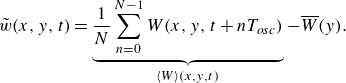 \begin{align} &\,\,\,\tilde {w}(x,y,t) = \underbrace {\frac {1}{N}\sum _{n=0}^{N-1} W(x,y,t+nT_{osc})}_{\left \langle W \right \rangle (x,y,t)} - \overline {W}(y). \end{align}
Here, $\overline {W}$
is the plane- and time-averaged component of the spanwise velocity,
$\overline {W}$
is the plane- and time-averaged component of the spanwise velocity, $\tilde {w}$
is the harmonic component,
$\tilde {w}$
is the harmonic component, $w$
is the turbulent component and
$w$
is the turbulent component and $\left \langle W \right \rangle$
is the spanwise- and phase-averaged value of
$\left \langle W \right \rangle$
is the spanwise- and phase-averaged value of $W$
. For the streamwise and wall-normal velocities and the temperature field, the harmonic components are negligible compared with the turbulent components. Following Rouhi et al. (Reference Rouhi, Fu, Chandran, Zampiron, Smits and Marusic2023), we quantify the Stokes layer protrusion height
$W$
. For the streamwise and wall-normal velocities and the temperature field, the harmonic components are negligible compared with the turbulent components. Following Rouhi et al. (Reference Rouhi, Fu, Chandran, Zampiron, Smits and Marusic2023), we quantify the Stokes layer protrusion height $\ell ^*_{0.01}$
as the wall distance where
$\ell ^*_{0.01}$
as the wall distance where $\overline {\tilde {w}^2}^* = 0.01$
, and we locate the Stokes layer thickness
$\overline {\tilde {w}^2}^* = 0.01$
, and we locate the Stokes layer thickness $\delta ^*_S$
where
$\delta ^*_S$
where $\overline { \tilde {w}^2}^* = ({1}/{2}){A^*}^2\textrm{e}^{-2}$
. We also calculate the production due to the Stokes layer according to
$\overline { \tilde {w}^2}^* = ({1}/{2}){A^*}^2\textrm{e}^{-2}$
. We also calculate the production due to the Stokes layer according to $P^*_{33} \equiv -2 \overline {\left \langle w v \right \rangle \partial \tilde {w}/\partial y }^*-2 \overline {\left \langle w u \right \rangle \partial \tilde {w}/\partial x}^*$
, where
$P^*_{33} \equiv -2 \overline {\left \langle w v \right \rangle \partial \tilde {w}/\partial y }^*-2 \overline {\left \langle w u \right \rangle \partial \tilde {w}/\partial x}^*$
, where $P^*_{33}$
is the only external source term due to the Stokes layer that injects energy into the turbulent stress budgets (Touber & Leschziner Reference Touber and Leschziner2012; Umair et al. Reference Umair, Tardu and Doche2022).
$P^*_{33}$
is the only external source term due to the Stokes layer that injects energy into the turbulent stress budgets (Touber & Leschziner Reference Touber and Leschziner2012; Umair et al. Reference Umair, Tardu and Doche2022).
The behaviour of these Stokes layer parameters is given in figure 15 for the same travelling wave cases shown in figure 5(a,c,e). The profiles do not depend on $Pr$
, that is, at a fixed
$Pr$
, that is, at a fixed $\omega ^+$
the Stokes layer structure remains unchanged as the Prandtl number changes. When
$\omega ^+$
the Stokes layer structure remains unchanged as the Prandtl number changes. When $\omega ^+$
decreases,
$\omega ^+$
decreases, $\ell ^*_{0.01}$
and the maximum production increase proportionately (figure 15
c). In other words, the Stokes layer becomes more protrusive while injecting more energy into the turbulent field. We note that
$\ell ^*_{0.01}$
and the maximum production increase proportionately (figure 15
c). In other words, the Stokes layer becomes more protrusive while injecting more energy into the turbulent field. We note that $\ell ^*_{0.01}$
is almost linearly proportional to
$\ell ^*_{0.01}$
is almost linearly proportional to $P^*_{{33}_{{max}}}$
, but
$P^*_{{33}_{{max}}}$
, but $\delta ^*_S$
is less responsive to the rise in the production. Therefore,
$\delta ^*_S$
is less responsive to the rise in the production. Therefore, $\ell ^*_{0.01}$
better quantifies the Stokes layer protrusion and strength, as sensed by the turbulent field, in agreement with the observations by Rouhi et al. (Reference Rouhi, Fu, Chandran, Zampiron, Smits and Marusic2023).
$\ell ^*_{0.01}$
better quantifies the Stokes layer protrusion and strength, as sensed by the turbulent field, in agreement with the observations by Rouhi et al. (Reference Rouhi, Fu, Chandran, Zampiron, Smits and Marusic2023).
Variation of the integral parameters with the Stokes layer characteristics $(\ell ^*_{0.01}, P^*_{{33}_{{max}}})$
for the same travelling wave cases as in figure 15. Plot (a) shows DR (blue squares), HR (light orange to brick red squares) versus
$(\ell ^*_{0.01}, P^*_{{33}_{{max}}})$
for the same travelling wave cases as in figure 15. Plot (a) shows DR (blue squares), HR (light orange to brick red squares) versus $\omega ^+$
. (b) Same data as in (a) versus
$\omega ^+$
. (b) Same data as in (a) versus $\ell ^*_{0.01}$
(bottom axis) and
$\ell ^*_{0.01}$
(bottom axis) and $P^*_{{33}_{{max}}}$
(top axis). Plots (c,d) correspond to (a,b) for
$P^*_{{33}_{{max}}}$
(top axis). Plots (c,d) correspond to (a,b) for $I_{uv}$
(blue squares) and
$I_{uv}$
(blue squares) and $I_{\theta v}$
(light orange to brick red squares); in (d) we overlay
$I_{\theta v}$
(light orange to brick red squares); in (d) we overlay $\gamma$
(grey to black triangles). In all plots, the colour of HR and
$\gamma$
(grey to black triangles). In all plots, the colour of HR and $I_{\theta v}$
changes from light orange at
$I_{\theta v}$
changes from light orange at $Pr=0.71$
to brick red at
$Pr=0.71$
to brick red at $Pr = 7.5$
. The points associated with
$Pr = 7.5$
. The points associated with ${\textrm{DR}}_{{max}}$
and
${\textrm{DR}}_{{max}}$
and ${\textrm{HR}}_{{max}}$
are highlighted with a larger symbol size and black outline. In (b,d) the grey region shades the range of
${\textrm{HR}}_{{max}}$
are highlighted with a larger symbol size and black outline. In (b,d) the grey region shades the range of ${\textrm{DR}}_{{max}}$
and
${\textrm{DR}}_{{max}}$
and ${\textrm{HR}}_{{max}}$
. In all plots we highlight two cases that we further analyse in figures 17 and 18: case A at
${\textrm{HR}}_{{max}}$
. In all plots we highlight two cases that we further analyse in figures 17 and 18: case A at $\omega ^+ = 0.088$
with
$\omega ^+ = 0.088$
with $\gamma = 0.16$
and case B at
$\gamma = 0.16$
and case B at $\omega ^+ = 0.022$
with
$\omega ^+ = 0.022$
with $\gamma = 0.53$
.
$\gamma = 0.53$
.
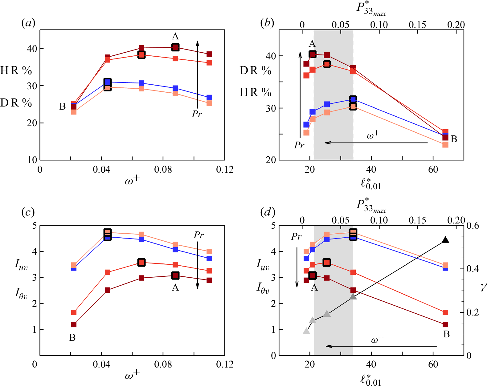
In figure 16 we assess the relation between the integral quantities DR, HR, $I_{\theta v}$
,
$I_{\theta v}$
, $I_{uv}$
and the Stokes layer characteristics. Rouhi et al. (Reference Rouhi, Fu, Chandran, Zampiron, Smits and Marusic2023) showed that DR increases with
$I_{uv}$
and the Stokes layer characteristics. Rouhi et al. (Reference Rouhi, Fu, Chandran, Zampiron, Smits and Marusic2023) showed that DR increases with $\ell ^*_{0.01}$
up to an optimal value for maximum DR, corresponding to an optimal level of
$\ell ^*_{0.01}$
up to an optimal value for maximum DR, corresponding to an optimal level of $P^*_{{33}_{{max}}}$
. For our present cases, this optimal point is
$P^*_{{33}_{{max}}}$
. For our present cases, this optimal point is $\ell ^*_{0.01} = 34$
(figure 16
b), where protrusion beyond this point causes DR to decrease. We observe a similar trend in HR (figure 16
b), but the corresponding optimal value of
$\ell ^*_{0.01} = 34$
(figure 16
b), where protrusion beyond this point causes DR to decrease. We observe a similar trend in HR (figure 16
b), but the corresponding optimal value of $\ell ^*_{0.01}$
for maximum HR decreases from 34to 21 as the Prandtl number increases from 0.71to 7.5. Figure 16(c,d) shows that the variations of
$\ell ^*_{0.01}$
for maximum HR decreases from 34to 21 as the Prandtl number increases from 0.71to 7.5. Figure 16(c,d) shows that the variations of $I_{uv}$
and
$I_{uv}$
and $I_{\theta v}$
with
$I_{\theta v}$
with $\omega ^+$
and
$\omega ^+$
and $\ell ^*_{0.01}$
are consistent with the trends in DR and HR. In terms of variations with
$\ell ^*_{0.01}$
are consistent with the trends in DR and HR. In terms of variations with $Pr$
, however, HR increases even as
$Pr$
, however, HR increases even as $I_{\theta v}$
decreases. From
$I_{\theta v}$
decreases. From $Pr=0.71$
to
$Pr=0.71$
to $7.5$
, the maximum value of
$7.5$
, the maximum value of $I_{\theta v}$
shifts to smaller values of
$I_{\theta v}$
shifts to smaller values of $\ell ^*_{0.01}$
, corresponding to a shift in
$\ell ^*_{0.01}$
, corresponding to a shift in $\omega ^+$
from 0.044 (
$\omega ^+$
from 0.044 ( $\ell ^*_{0.01} = 34$
) to 0.088 (
$\ell ^*_{0.01} = 34$
) to 0.088 ( $\ell ^*_{0.01} = 21$
). Finally, it appears that the exponent
$\ell ^*_{0.01} = 21$
). Finally, it appears that the exponent $\gamma$
in the power law increases almost linearly with
$\gamma$
in the power law increases almost linearly with $\ell ^*_{0.01}$
and
$\ell ^*_{0.01}$
and $P^*_{33_{{max}}}$
(figure 16
d).
$P^*_{33_{{max}}}$
(figure 16
d).
To summarise, we find that for $Pr \gt 1$
, achieving maximum HR requires a less protrusive Stokes layer than achieving maximum DR. As the Stokes layer becomes more protrusive (energetic), it loses its efficacy in attenuating
$Pr \gt 1$
, achieving maximum HR requires a less protrusive Stokes layer than achieving maximum DR. As the Stokes layer becomes more protrusive (energetic), it loses its efficacy in attenuating $\overline {\theta v}^*$
relative to
$\overline {\theta v}^*$
relative to $\overline {u v}^*$
, that is,
$\overline {u v}^*$
, that is, $\gamma$
increases as
$\gamma$
increases as $\ell ^*_{0.01}$
increases.
$\ell ^*_{0.01}$
increases.
3.7. Stokes layer interaction with the velocity and thermal fields: scale-wise analysis
To better understand our observations on the integral parameters shown in figure 16, we now examine the spectrograms of $\overline {u v}^*$
and
$\overline {u v}^*$
and $\overline {\theta v}^*$
and visualise the distributions of the instantaneous
$\overline {\theta v}^*$
and visualise the distributions of the instantaneous $u v$
and
$u v$
and $\theta v$
near the wall. We focus on two cases at
$\theta v$
near the wall. We focus on two cases at $Pr = 7.5$
, case A at
$Pr = 7.5$
, case A at $\omega ^+ = 0.088$
, where HR is maximum and DR is near maximum (
$\omega ^+ = 0.088$
, where HR is maximum and DR is near maximum ( $\gamma = 0.16$
), and case B at
$\gamma = 0.16$
), and case B at $\omega ^+ = 0.022$
, where HR and DR drop below their maximum values, owing to a highly protrusive Stokes layer (
$\omega ^+ = 0.022$
, where HR and DR drop below their maximum values, owing to a highly protrusive Stokes layer ( $\gamma = 0.53$
).
$\gamma = 0.53$
).
Figure 17 displays the various pre-multiplied spectrograms for these two cases, where $\phi$
is the spectral density,
$\phi$
is the spectral density, $k_x$
is the streamwise wavenumber,
$k_x$
is the streamwise wavenumber, $k_z$
is the spanwise wavenumber and
$k_z$
is the spanwise wavenumber and $f$
is the frequency. The differences between the actuated and non-actuated cases are denoted by, for example,
$f$
is the frequency. The differences between the actuated and non-actuated cases are denoted by, for example, $\unicode{x1D6E5} k^*_x \phi ^*_{uv} = k^*_x \phi ^*_{uv} - k^*_x \phi ^*_{{uv}_0}$
. The extent up to which
$\unicode{x1D6E5} k^*_x \phi ^*_{uv} = k^*_x \phi ^*_{uv} - k^*_x \phi ^*_{{uv}_0}$
. The extent up to which $\unicode{x1D6E5} k^*_x \phi ^*_{uv}$
and
$\unicode{x1D6E5} k^*_x \phi ^*_{uv}$
and $\unicode{x1D6E5} k^*_x \phi ^*_{\theta v}$
are non-zero (red and blue fields in figure 17
e,f,q,r) coincides with the height of the Stokes layer protrusion
$\unicode{x1D6E5} k^*_x \phi ^*_{\theta v}$
are non-zero (red and blue fields in figure 17
e,f,q,r) coincides with the height of the Stokes layer protrusion $\ell ^*_{0.01}$
(horizontal dashed line); this supports the robustness of
$\ell ^*_{0.01}$
(horizontal dashed line); this supports the robustness of $\ell ^*_{0.01}$
to measure the extent up to which the Stokes layer modifies the turbulent field. Overall, for both cases A and B, and
$\ell ^*_{0.01}$
to measure the extent up to which the Stokes layer modifies the turbulent field. Overall, for both cases A and B, and $k^*_x \phi ^*_{uv}$
and
$k^*_x \phi ^*_{uv}$
and $ k^*_x \phi ^*_{\theta v}$
, the Stokes layer protrusion (production) leads to two outcomes: (i) large-scale energy attenuation as a favourable outcome (positive
$ k^*_x \phi ^*_{\theta v}$
, the Stokes layer protrusion (production) leads to two outcomes: (i) large-scale energy attenuation as a favourable outcome (positive $\unicode{x1D6E5} k^*_x \phi ^*_{uv}, \unicode{x1D6E5} k^*_x \phi ^*_{\theta v}$
for
$\unicode{x1D6E5} k^*_x \phi ^*_{uv}, \unicode{x1D6E5} k^*_x \phi ^*_{\theta v}$
for $\lambda ^*_x \gtrsim 350$
, shown as the red fields in figure 17
e,f,q,r), and (ii) small-scale energy amplification as an unfavourable outcome (negative
$\lambda ^*_x \gtrsim 350$
, shown as the red fields in figure 17
e,f,q,r), and (ii) small-scale energy amplification as an unfavourable outcome (negative $\unicode{x1D6E5} k^*_x \phi ^*_{uv}, \unicode{x1D6E5} k^*_x \phi ^*_{\theta v}$
for
$\unicode{x1D6E5} k^*_x \phi ^*_{uv}, \unicode{x1D6E5} k^*_x \phi ^*_{\theta v}$
for $\lambda ^*_x \lesssim 350$
, shown as the blue fields). The large-scale energy attenuation corresponds to the attenuation of the near-wall streaks with
$\lambda ^*_x \lesssim 350$
, shown as the blue fields). The large-scale energy attenuation corresponds to the attenuation of the near-wall streaks with $\lambda ^*_x \simeq 10^3$
(see the energetic peaks in the non-actuated spectrograms). The small-scale energy amplification corresponds to the emergence of smaller scales with
$\lambda ^*_x \simeq 10^3$
(see the energetic peaks in the non-actuated spectrograms). The small-scale energy amplification corresponds to the emergence of smaller scales with $\lambda ^*_x \simeq 10^2$
(figure 18
j,k,l,m,u,v,w,x). The drastic changes in the streamwise spectrograms (figure 17
e,f,q,r) are echoed in the response of the frequency spectrograms (figure 17
g,h,s,t). Changing the actuation frequency
$\lambda ^*_x \simeq 10^2$
(figure 18
j,k,l,m,u,v,w,x). The drastic changes in the streamwise spectrograms (figure 17
e,f,q,r) are echoed in the response of the frequency spectrograms (figure 17
g,h,s,t). Changing the actuation frequency $\omega ^+$
, hence changing the Stokes layer time scale, modifies the near-wall turbulence time scale
$\omega ^+$
, hence changing the Stokes layer time scale, modifies the near-wall turbulence time scale $T^*$
, which in turn modifies the streamwise length scale
$T^*$
, which in turn modifies the streamwise length scale $\lambda ^*_x$
(of course,
$\lambda ^*_x$
(of course, $T^*$
is related to
$T^*$
is related to $\lambda ^*_x$
through a convection speed of approximately
$\lambda ^*_x$
through a convection speed of approximately $ \mathcal{O}(10)$
according to Taylor’s hypothesis).
$ \mathcal{O}(10)$
according to Taylor’s hypothesis).
Further insight can be gained by comparing the near-wall instantaneous fields of $u^* v^*$
and
$u^* v^*$
and $\theta ^* v^*$
, as shown in figure 18. The response of
$\theta ^* v^*$
, as shown in figure 18. The response of $u^* v^*$
to the Stokes layer (blue intensity fields) largely follows the trends seen in
$u^* v^*$
to the Stokes layer (blue intensity fields) largely follows the trends seen in $\unicode{x1D6E5} k^*_x \phi ^*_{uv}$
and
$\unicode{x1D6E5} k^*_x \phi ^*_{uv}$
and $ \unicode{x1D6E5} f^* \phi ^*_{uv}$
. For case A, we see that the large scales associated with the near-wall streaks are attenuated. At the same time, sparse patches of smaller scales with
$ \unicode{x1D6E5} f^* \phi ^*_{uv}$
. For case A, we see that the large scales associated with the near-wall streaks are attenuated. At the same time, sparse patches of smaller scales with $\lambda ^*_x \simeq 10^2$
(
$\lambda ^*_x \simeq 10^2$
( $T^* \simeq 10$
) emerge. For case B, the emerging smaller scales possess a similar structure and size to those in case A, but with a noticeably larger population; they appear as large and closely spaced patches that cover a significant area of the near-wall region. Consistently, negative regions of
$T^* \simeq 10$
) emerge. For case B, the emerging smaller scales possess a similar structure and size to those in case A, but with a noticeably larger population; they appear as large and closely spaced patches that cover a significant area of the near-wall region. Consistently, negative regions of $\unicode{x1D6E5} k^*_x \phi ^*_{uv}$
and
$\unicode{x1D6E5} k^*_x \phi ^*_{uv}$
and $ \unicode{x1D6E5} f^* \phi ^*_{uv}$
are small for case A (figure 17
e,g), and large for case B (figure 17
q,s). Thus,
$ \unicode{x1D6E5} f^* \phi ^*_{uv}$
are small for case A (figure 17
e,g), and large for case B (figure 17
q,s). Thus, $I_{uv}$
and DR are greater for case A than for case B (figure 16). Attenuation of the large scales associated with the near-wall streaks is considered to be a primary source of DR, as extensively reported in the literature (Baron & Quadrio Reference Baron and Quadrio1995; Di Cicca et al. Reference Di Cicca, Iuso, Spazzini and Onorato2002; Karniadakis & Choi Reference Karniadakis and Choi2003; Ricco Reference Ricco2004; Quadrio et al. Reference Quadrio, Ricco and Viotti2009; Touber & Leschziner Reference Touber and Leschziner2012; Ricco et al. Reference Ricco, Skote and Leschziner2021; Marusic et al. Reference Marusic, Chandran, Rouhi, Fu, Wine, Holloway, Chung and Smits2021; Rouhi et al. Reference Rouhi, Fu, Chandran, Zampiron, Smits and Marusic2023). However, amplification of the smaller scales as a source of drag increase, is reported to a lesser extent. Touber & Leschziner (Reference Touber and Leschziner2012) observed such amplification in the frequency spectrograms
$I_{uv}$
and DR are greater for case A than for case B (figure 16). Attenuation of the large scales associated with the near-wall streaks is considered to be a primary source of DR, as extensively reported in the literature (Baron & Quadrio Reference Baron and Quadrio1995; Di Cicca et al. Reference Di Cicca, Iuso, Spazzini and Onorato2002; Karniadakis & Choi Reference Karniadakis and Choi2003; Ricco Reference Ricco2004; Quadrio et al. Reference Quadrio, Ricco and Viotti2009; Touber & Leschziner Reference Touber and Leschziner2012; Ricco et al. Reference Ricco, Skote and Leschziner2021; Marusic et al. Reference Marusic, Chandran, Rouhi, Fu, Wine, Holloway, Chung and Smits2021; Rouhi et al. Reference Rouhi, Fu, Chandran, Zampiron, Smits and Marusic2023). However, amplification of the smaller scales as a source of drag increase, is reported to a lesser extent. Touber & Leschziner (Reference Touber and Leschziner2012) observed such amplification in the frequency spectrograms $f^*\phi ^*_{uu}$
,
$f^*\phi ^*_{uu}$
, $f^*\phi ^*_{vv}$
and
$f^*\phi ^*_{vv}$
and $f^*\phi ^*_{ww}$
. Consistent with our figure 17, they noted that as
$f^*\phi ^*_{ww}$
. Consistent with our figure 17, they noted that as $\omega ^+$
changes from 0.06to 0.03, and the Stokes layer production (protrusion) increases, energy accumulates in the scales with
$\omega ^+$
changes from 0.06to 0.03, and the Stokes layer production (protrusion) increases, energy accumulates in the scales with $T^* \simeq 10$
and DR decreases. Similarly, energy amplification at
$T^* \simeq 10$
and DR decreases. Similarly, energy amplification at $T^* \simeq 10$
is observed in
$T^* \simeq 10$
is observed in $f^*\phi ^*_{\tau \tau }$
by Chandran et al. (Reference Chandran, Zampiron, Rouhi, Fu, Wine, Holloway, Smits and Marusic2023), and in the near-wall
$f^*\phi ^*_{\tau \tau }$
by Chandran et al. (Reference Chandran, Zampiron, Rouhi, Fu, Wine, Holloway, Smits and Marusic2023), and in the near-wall $f^* \phi ^*_{uu}$
by Deshpande et al. (Reference Deshpande, Chandran, Smits and Marusic2023).
$f^* \phi ^*_{uu}$
by Deshpande et al. (Reference Deshpande, Chandran, Smits and Marusic2023).
Comparisons between case A (left two columns) and case B (right two columns. (a,m) Profiles of $\unicode{x1D6E5} ^*_{uv}$
(blue) and
$\unicode{x1D6E5} ^*_{uv}$
(blue) and $\unicode{x1D6E5} ^*_{\theta v}$
(red). (b,n) Profiles of
$\unicode{x1D6E5} ^*_{\theta v}$
(red). (b,n) Profiles of $\overline { \tilde {w}^2}^*$
(dashed-dotted line) and
$\overline { \tilde {w}^2}^*$
(dashed-dotted line) and $P^*_{33}$
(solid line). Streamwise spectrograms: (c,o)
$P^*_{33}$
(solid line). Streamwise spectrograms: (c,o) $-k^*_x\phi ^*_{uv}$
; (d,p)
$-k^*_x\phi ^*_{uv}$
; (d,p) $-k^*_x\phi ^*_{\theta v}$
(contour lines and contour fields represent non-actuated and actuated cases, respectively). Difference between the actuated and non-actuated cases for the wavenumber spectra (e,f,q,r) and frequency spectra (g,h,s,t). Spanwise spectrograms: (i,u)
$-k^*_x\phi ^*_{\theta v}$
(contour lines and contour fields represent non-actuated and actuated cases, respectively). Difference between the actuated and non-actuated cases for the wavenumber spectra (e,f,q,r) and frequency spectra (g,h,s,t). Spanwise spectrograms: (i,u) $-k^*_z\phi ^*_{uv}$
; (j,v)
$-k^*_z\phi ^*_{uv}$
; (j,v) $-k^*_z\phi ^*_{\theta v}$
. Difference between the actuated and non-actuated cases (k,l,w,x). In all the spectrgrams, the horizontal dashed line marks
$-k^*_z\phi ^*_{\theta v}$
. Difference between the actuated and non-actuated cases (k,l,w,x). In all the spectrgrams, the horizontal dashed line marks $\ell ^*_{0.01}$
.
$\ell ^*_{0.01}$
.
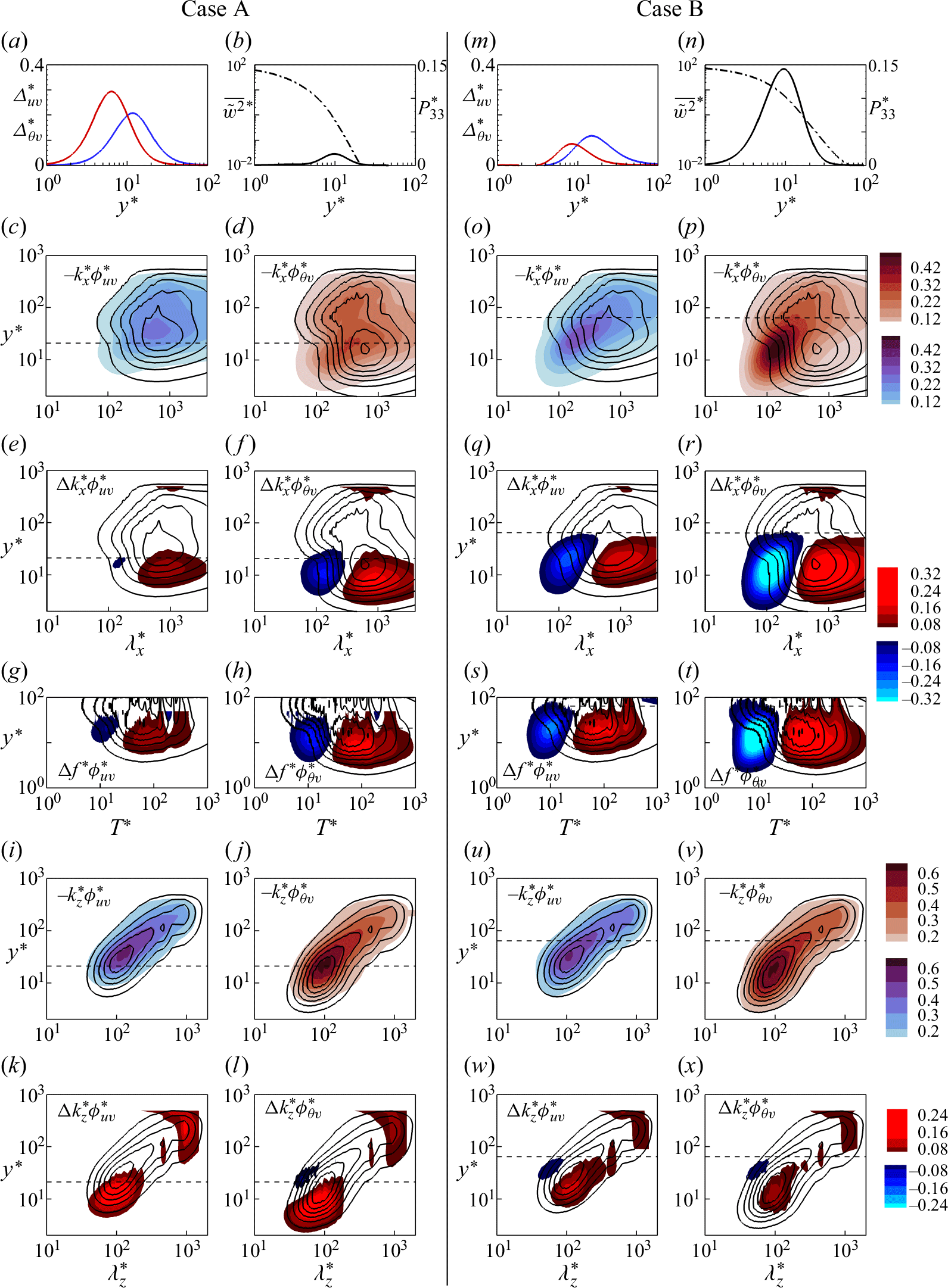
Visualisations of the instantaneous fields of $u^* v^*$
(blue intensity fields) and
$u^* v^*$
(blue intensity fields) and $\theta ^* v^*$
(brick intensity fields) at
$\theta ^* v^*$
(brick intensity fields) at $y^+ = 14$
for the same cases as in figure 17. Next to each field, we magnify the small square outlined in pink. Left: non-actuated case; middle: actuated case A; right: actuated case B. The top two rows visualise
$y^+ = 14$
for the same cases as in figure 17. Next to each field, we magnify the small square outlined in pink. Left: non-actuated case; middle: actuated case A; right: actuated case B. The top two rows visualise $u^* v^*$
and
$u^* v^*$
and $\theta ^* v^*$
at one time over the
$\theta ^* v^*$
at one time over the $x^*$
-
$x^*$
- $z^*$
plane. (i,t) Plot of the corresponding spanwise wall velocity
$z^*$
plane. (i,t) Plot of the corresponding spanwise wall velocity $W^*_s$
over
$W^*_s$
over $x^*$
at the same time. The bottom two rows visualise
$x^*$
at the same time. The bottom two rows visualise $u^* v^*$
and
$u^* v^*$
and $\theta ^* v^*$
at one
$\theta ^* v^*$
at one $x^*$
location over
$x^*$
location over $z^*$
and time
$z^*$
and time $t^*$
. (o,y) Plot of
$t^*$
. (o,y) Plot of $W^*_s$
over
$W^*_s$
over $t^*$
at the same
$t^*$
at the same $x^*$
location.
$x^*$
location.
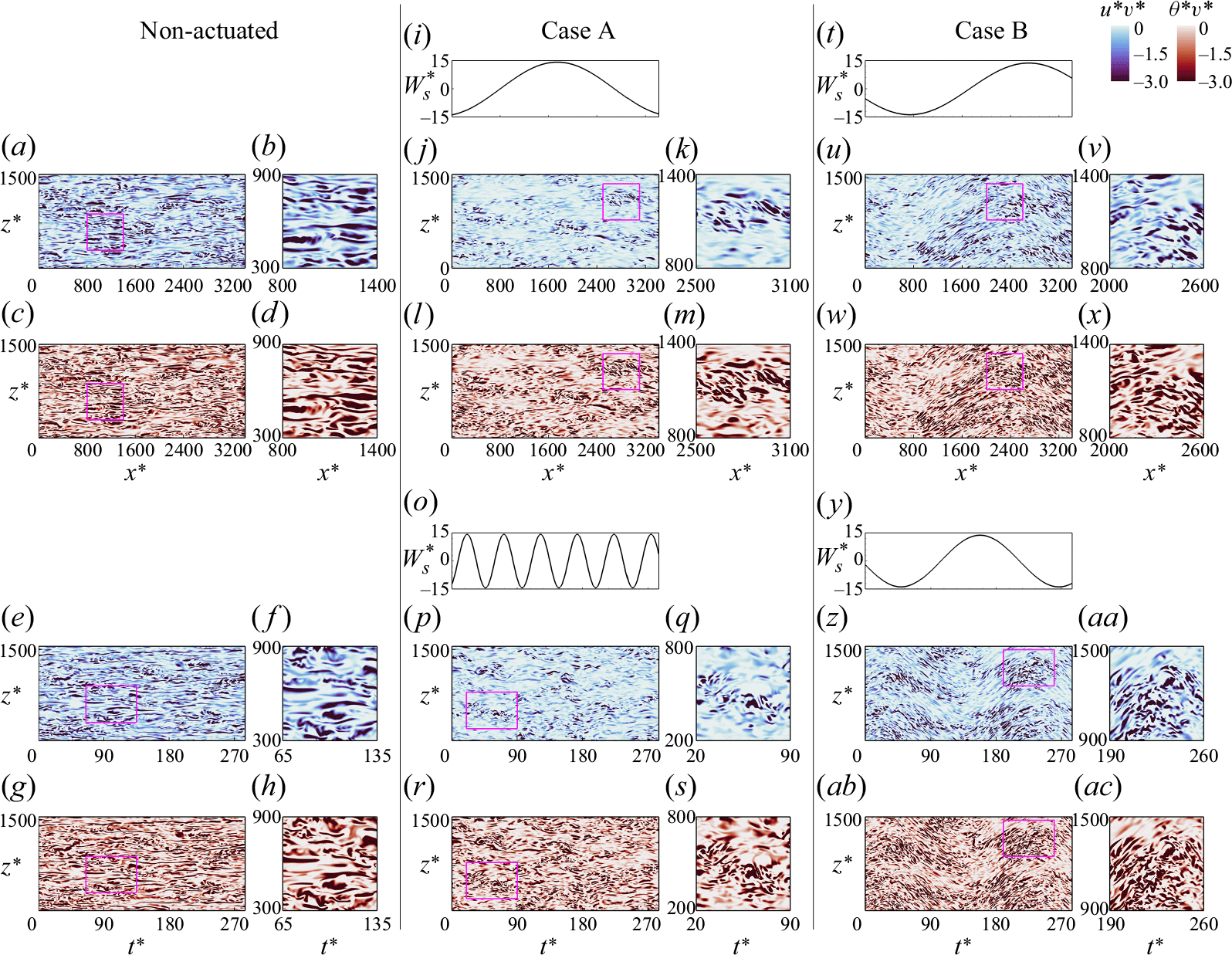
As to the $\theta ^* v^*$
field (brick intensity fields in figure 18), we see that with
$\theta ^* v^*$
field (brick intensity fields in figure 18), we see that with $Pr \gt 1.0$
the Stokes layer modifies the
$Pr \gt 1.0$
the Stokes layer modifies the $\theta ^* v^*$
field more than the
$\theta ^* v^*$
field more than the $u^* v^*$
field. In case A, for example, the scales with
$u^* v^*$
field. In case A, for example, the scales with $\lambda ^*_x \simeq 10^2$
and
$\lambda ^*_x \simeq 10^2$
and $T^* \simeq 10$
are more frequent and more densely populated in the
$T^* \simeq 10$
are more frequent and more densely populated in the $\theta ^* v^*$
fields (figure 18
l,m,r,s) than in the
$\theta ^* v^*$
fields (figure 18
l,m,r,s) than in the $u^* v^*$
fields (figure 18
j,k,p,q). Consistently,
$u^* v^*$
fields (figure 18
j,k,p,q). Consistently, $\unicode{x1D6E5} k^*_x\phi ^*_{\theta v}$
(figure 17
f) is more positive than
$\unicode{x1D6E5} k^*_x\phi ^*_{\theta v}$
(figure 17
f) is more positive than $\unicode{x1D6E5} k^*_x\phi ^*_{u v}$
(figure 17
e) for
$\unicode{x1D6E5} k^*_x\phi ^*_{u v}$
(figure 17
e) for $\lambda ^*_x \gtrsim 350$
, and more negative for
$\lambda ^*_x \gtrsim 350$
, and more negative for $\lambda ^*_x \lesssim 350$
. We can make the same observations with respect to case B (figure 17
q,r). As a result, at each
$\lambda ^*_x \lesssim 350$
. We can make the same observations with respect to case B (figure 17
q,r). As a result, at each $\omega ^+$
,
$\omega ^+$
, $I_{\theta v}$
falls below
$I_{\theta v}$
falls below $I_{uv}$
when
$I_{uv}$
when $Pr \gt 1$
(figure 16
c,d).
$Pr \gt 1$
(figure 16
c,d).
At a fixed $\omega ^+$
,
$\omega ^+$
, $u^* v^*$
and
$u^* v^*$
and $\theta ^* v^*$
are exposed to an identical Stokes layer. However, the larger change in
$\theta ^* v^*$
are exposed to an identical Stokes layer. However, the larger change in $\unicode{x1D6E5} k^*_x \phi ^*_{\theta v}$
compared with
$\unicode{x1D6E5} k^*_x \phi ^*_{\theta v}$
compared with $\unicode{x1D6E5} k^*_x \phi ^*_{u v}$
for
$\unicode{x1D6E5} k^*_x \phi ^*_{u v}$
for $Pr \gt 1$
implies that the energetic near-wall scales of
$Pr \gt 1$
implies that the energetic near-wall scales of $\theta ^* v^*$
are locally exposed to a stronger Stokes layer production. We establish this connection by evaluating the local Stokes layer production
$\theta ^* v^*$
are locally exposed to a stronger Stokes layer production. We establish this connection by evaluating the local Stokes layer production $P^*_{33p}$
at the negative peaks of
$P^*_{33p}$
at the negative peaks of $\unicode{x1D6E5} k^*_x \phi ^*_{\theta v}$
and
$\unicode{x1D6E5} k^*_x \phi ^*_{\theta v}$
and $\unicode{x1D6E5} k^*_x \phi ^*_{u v}$
; these peaks are associated with the energetic small scales with
$\unicode{x1D6E5} k^*_x \phi ^*_{u v}$
; these peaks are associated with the energetic small scales with $\lambda ^*_x \simeq 10^2$
that contribute to the drop in
$\lambda ^*_x \simeq 10^2$
that contribute to the drop in $I_{uv}$
and
$I_{uv}$
and $I_{\theta v}$
. Figure 19(b) demonstrates this process for case B (figure 17
r), where the negative peak of
$I_{\theta v}$
. Figure 19(b) demonstrates this process for case B (figure 17
r), where the negative peak of $\unicode{x1D6E5} k^*_x \phi ^*_{\theta v}$
is intersected with the
$\unicode{x1D6E5} k^*_x \phi ^*_{\theta v}$
is intersected with the $P^*_{33}$
profile. With increasing
$P^*_{33}$
profile. With increasing $Pr$
, the conductive sublayer thins and the negative peak in
$Pr$
, the conductive sublayer thins and the negative peak in $\unicode{x1D6E5} k^*_x \phi ^*_{\theta v}$
falls closer to the wall compared with its counterpart from
$\unicode{x1D6E5} k^*_x \phi ^*_{\theta v}$
falls closer to the wall compared with its counterpart from $\unicode{x1D6E5} k^*_x \phi ^*_{u v}$
. This means that at each
$\unicode{x1D6E5} k^*_x \phi ^*_{u v}$
. This means that at each $\omega ^+$
, the energetic small scales of
$\omega ^+$
, the energetic small scales of $\theta ^* v^*$
are exposed to a larger Stokes layer production, and hence, have a higher energy. This leads to the drop in
$\theta ^* v^*$
are exposed to a larger Stokes layer production, and hence, have a higher energy. This leads to the drop in $I_{\theta v}$
compared with
$I_{\theta v}$
compared with $I_{uv}$
, as demonstrated in figure 19(a). At
$I_{uv}$
, as demonstrated in figure 19(a). At $Pr = 0.71$
, the local production
$Pr = 0.71$
, the local production $P^*_{33p}$
is close between
$P^*_{33p}$
is close between $u^* v^*$
and
$u^* v^*$
and $\theta ^* v^*$
, and
$\theta ^* v^*$
, and $I_{uv}$
and
$I_{uv}$
and $I_{\theta v}$
are close to each other. However, at
$I_{\theta v}$
are close to each other. However, at $Pr = 4.0$
and
$Pr = 4.0$
and $7.5$
,
$7.5$
, $P^*_{33p}$
at each
$P^*_{33p}$
at each $\omega ^+$
is several times higher for
$\omega ^+$
is several times higher for $\theta ^* v^*$
than
$\theta ^* v^*$
than $u^* v^*$
, and
$u^* v^*$
, and $I_{\theta v}$
drops below
$I_{\theta v}$
drops below $I_{u v}$
. In addition, at
$I_{u v}$
. In addition, at $\omega ^+ = 0.022$
,
$\omega ^+ = 0.022$
, $P^*_{33p}$
increases by almost 3 times from
$P^*_{33p}$
increases by almost 3 times from $Pr = 0.71$
to
$Pr = 0.71$
to $7.5$
, whereas at
$7.5$
, whereas at $\omega ^+ = 0.110$
,
$\omega ^+ = 0.110$
, $P^*_{33p}$
increases by
$P^*_{33p}$
increases by $1.5$
times. As a result,
$1.5$
times. As a result, $I_{\theta v}$
has a milder decay rate at
$I_{\theta v}$
has a milder decay rate at $\omega ^+ = 0.110$
(
$\omega ^+ = 0.110$
( $\gamma = 0.11$
) than at
$\gamma = 0.11$
) than at $\omega ^+ = 0.022$
(
$\omega ^+ = 0.022$
( $\gamma = 0.53$
).
$\gamma = 0.53$
).
Assessment of the relation between $I_{uv}$
and
$I_{uv}$
and $I_{\theta v}$
, and the local Stokes layer production
$I_{\theta v}$
, and the local Stokes layer production $P^*_{33p}$
at the negative peaks of
$P^*_{33p}$
at the negative peaks of $\unicode{x1D6E5} k^*_x \phi ^*_{uv}$
and
$\unicode{x1D6E5} k^*_x \phi ^*_{uv}$
and $\unicode{x1D6E5} k^*_x \phi ^*_{\theta v}$
. (a) Same data of
$\unicode{x1D6E5} k^*_x \phi ^*_{\theta v}$
. (a) Same data of $I_{uv}$
and
$I_{uv}$
and $I_{\theta v}$
as in figure 16(c), but versus
$I_{\theta v}$
as in figure 16(c), but versus $P^*_{33p}$
; to ease the inspection, the inset shows figure 16(c). The data points at
$P^*_{33p}$
; to ease the inspection, the inset shows figure 16(c). The data points at $\omega ^+ = 0.022$
and
$\omega ^+ = 0.022$
and $0.110$
have black and grey outlines, respectively. Panel (b) illustrates obtaining
$0.110$
have black and grey outlines, respectively. Panel (b) illustrates obtaining $P^*_{33p}$
for case B (figure 17
r), by intersecting the negative peak of
$P^*_{33p}$
for case B (figure 17
r), by intersecting the negative peak of $\unicode{x1D6E5} k^*_x \phi ^*_{\theta v}$
with the
$\unicode{x1D6E5} k^*_x \phi ^*_{\theta v}$
with the $P^*_{33}$
profile (on the left axis).
$P^*_{33}$
profile (on the left axis).
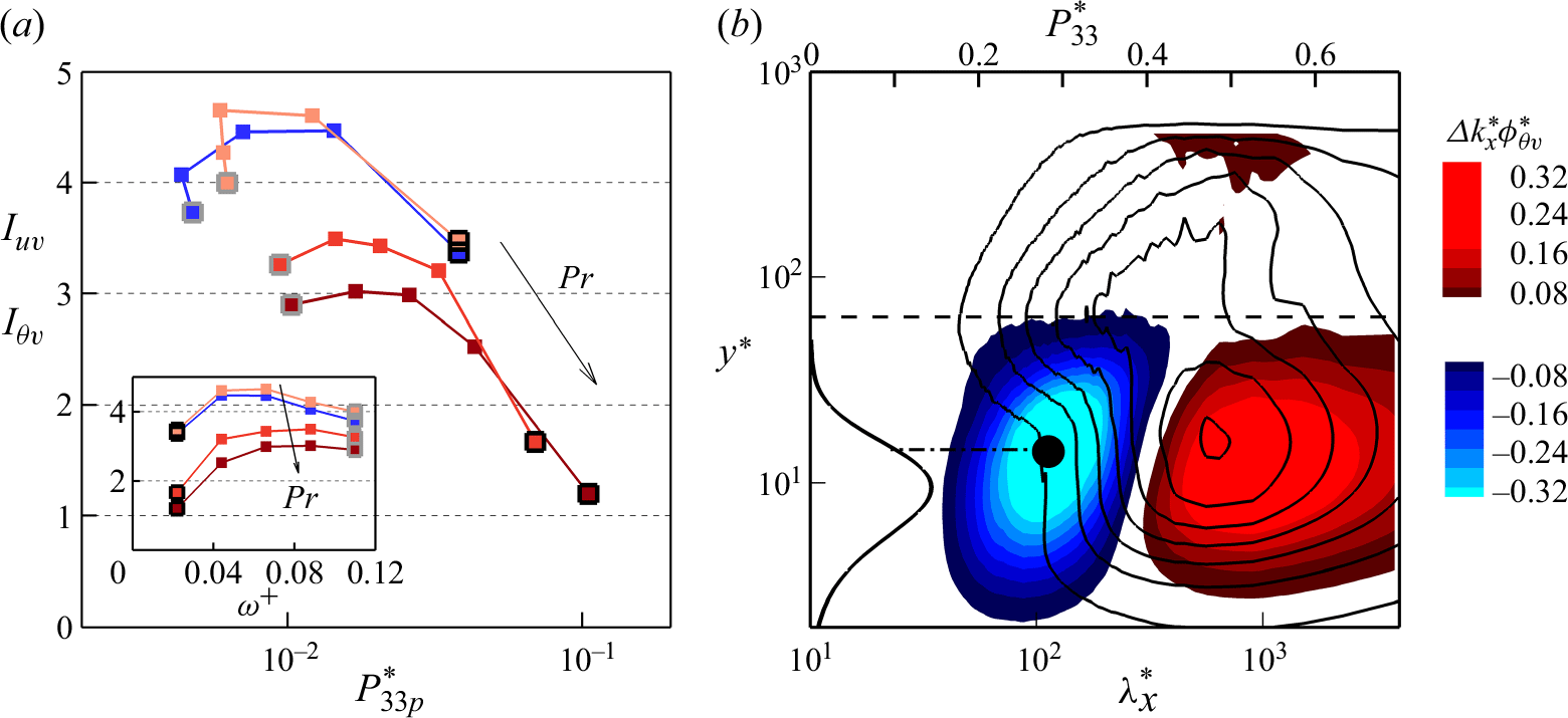
We have seen how the behaviour of the Stokes layer leads to $I_{\theta v}\lt I_{u v}$
by examining the streamwise and frequency spectrograms. This connection is more difficult to find in the spanwise spectrograms
$I_{\theta v}\lt I_{u v}$
by examining the streamwise and frequency spectrograms. This connection is more difficult to find in the spanwise spectrograms $k^*_z \phi ^*_{u v}$
and
$k^*_z \phi ^*_{u v}$
and $ k^*_z \phi ^*_{\theta v}$
(figure 17
i–l, u–x). The Stokes layer predominantly modifies the time scale
$ k^*_z \phi ^*_{\theta v}$
(figure 17
i–l, u–x). The Stokes layer predominantly modifies the time scale $T^*$
, hence, the streamwise length scale
$T^*$
, hence, the streamwise length scale $\lambda ^*_x$
, of the near-wall turbulence. However,
$\lambda ^*_x$
, of the near-wall turbulence. However, $k^*_z \phi ^*_{u v}$
and
$k^*_z \phi ^*_{u v}$
and $ k^*_z \phi ^*_{\theta v}$
are integrated over
$ k^*_z \phi ^*_{\theta v}$
are integrated over $T^*$
and
$T^*$
and $\lambda ^*_x$
, and so the small-scale energy amplification is cancelled by the large-scale energy attenuation. Thus, even though the Stokes layer protrusion (production) increases from case A to case B, the distributions of
$\lambda ^*_x$
, and so the small-scale energy amplification is cancelled by the large-scale energy attenuation. Thus, even though the Stokes layer protrusion (production) increases from case A to case B, the distributions of $k^*_z \phi ^*_{u v}$
and
$k^*_z \phi ^*_{u v}$
and $ k^*_z \phi ^*_{\theta v}$
suggest that the near-wall turbulence is distorted to a lesser extent.
$ k^*_z \phi ^*_{\theta v}$
suggest that the near-wall turbulence is distorted to a lesser extent.
Large- and small-scale contributions to $\unicode{x1D6E5} ^*_{uv}, \unicode{x1D6E5} ^*_{\theta v}$
and their integrals
$\unicode{x1D6E5} ^*_{uv}, \unicode{x1D6E5} ^*_{\theta v}$
and their integrals $I_{uv}, I_{\theta v}$
for the travelling wave case. Left column:
$I_{uv}, I_{\theta v}$
for the travelling wave case. Left column: $\omega ^+ = 0.088$
; middlecolumn:
$\omega ^+ = 0.088$
; middlecolumn: $\omega ^+ = 0.044$
; rightcolumn:
$\omega ^+ = 0.044$
; rightcolumn: $\omega ^+ = 0.022$
. Blue
$\omega ^+ = 0.022$
. Blue $uv$
profiles; for
$uv$
profiles; for $\theta v$
profiles,
$\theta v$
profiles, $Pr = 0.71$
is shown in light orange,
$Pr = 0.71$
is shown in light orange, $Pr = 4.0$
in orange and
$Pr = 4.0$
in orange and $Pr = 7.5$
in brick red. (a,b,c) Plot of
$Pr = 7.5$
in brick red. (a,b,c) Plot of $I_{uv}, I_{\theta v}$
versus
$I_{uv}, I_{\theta v}$
versus $\omega ^+$
. (d,e,f) Plot of
$\omega ^+$
. (d,e,f) Plot of $\unicode{x1D6E5} ^*_{uv}, \unicode{x1D6E5} ^*_{\theta v}$
versus
$\unicode{x1D6E5} ^*_{uv}, \unicode{x1D6E5} ^*_{\theta v}$
versus $y^*$
; the insets plot
$y^*$
; the insets plot $\overline {\tilde {w}^2}^*$
representing the Stokes layer where the number reports
$\overline {\tilde {w}^2}^*$
representing the Stokes layer where the number reports $\ell ^*_{0.01}$
. (d,e,f) Total
$\ell ^*_{0.01}$
. (d,e,f) Total $\unicode{x1D6E5} ^*_{uv} \unicode{x1D6E5} ^*_{\theta v}$
; (g,h,i) decomposed
$\unicode{x1D6E5} ^*_{uv} \unicode{x1D6E5} ^*_{\theta v}$
; (g,h,i) decomposed $\unicode{x1D6E5} ^*_{uv\pm }, \unicode{x1D6E5} ^*_{\theta v\pm }$
. In (d–i) we shade under the profiles of
$\unicode{x1D6E5} ^*_{uv\pm }, \unicode{x1D6E5} ^*_{\theta v\pm }$
. In (d–i) we shade under the profiles of $\unicode{x1D6E5} ^*_{uv}$
and
$\unicode{x1D6E5} ^*_{uv}$
and $\unicode{x1D6E5} ^*_{\theta v}$
at
$\unicode{x1D6E5} ^*_{\theta v}$
at $Pr = 7.5$
, as well as their decomposition.
$Pr = 7.5$
, as well as their decomposition.
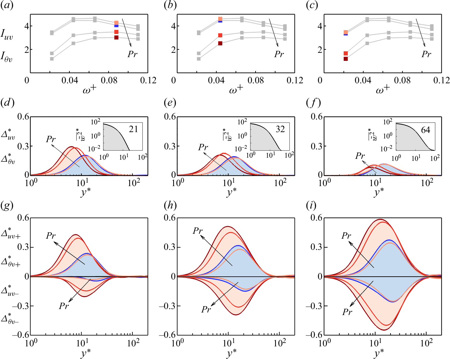
Our observations regarding the large-scale attenuation and small-scale amplification can be extended by applying scale-wise decomposition to $\unicode{x1D6E5} ^*_{uv}$
and
$\unicode{x1D6E5} ^*_{uv}$
and $ \unicode{x1D6E5} ^*_{\theta v}$
. For instance, we can write
$ \unicode{x1D6E5} ^*_{\theta v}$
. For instance, we can write $\unicode{x1D6E5} ^*_{uv} = \unicode{x1D6E5} ^*_{uv+} + \unicode{x1D6E5} ^*_{uv-}$
, where
$\unicode{x1D6E5} ^*_{uv} = \unicode{x1D6E5} ^*_{uv+} + \unicode{x1D6E5} ^*_{uv-}$
, where
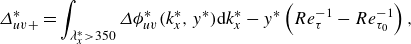 \begin{align} &\unicode{x1D6E5} ^*_{uv+} = \int _{\lambda ^*_x \gt 350} \unicode{x1D6E5} \phi ^*_{uv}(k^*_x,y^*) {\mathrm d}k^*_x - y^*\left (Re^{-1}_\tau - Re^{-1}_{\tau _0}\right ), \end{align}
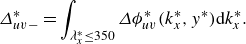 \begin{align} &\quad\qquad\qquad \unicode{x1D6E5} ^*_{uv-} = \int _{\lambda ^*_x \le 350} \unicode{x1D6E5} \phi ^*_{uv}(k^*_x,y^*) {\mathrm d}k^*_x. \end{align}
We set the threshold of $\lambda ^*_x = 350$
for partitioning because the spectrograms for all cases show
$\lambda ^*_x = 350$
for partitioning because the spectrograms for all cases show $\unicode{x1D6E5} k^*_x \phi ^*_{uv} \gt 0$
for
$\unicode{x1D6E5} k^*_x \phi ^*_{uv} \gt 0$
for $\lambda ^*_x \gtrsim 350$
and
$\lambda ^*_x \gtrsim 350$
and $\unicode{x1D6E5} k^*_x \phi ^*_{uv}\lt 0$
for
$\unicode{x1D6E5} k^*_x \phi ^*_{uv}\lt 0$
for $\lambda ^*_x \lesssim 350$
(see figure 17
e,q). As noted earlier (figure 10
a and (3.3a
)), we need to subtract the term
$\lambda ^*_x \lesssim 350$
(see figure 17
e,q). As noted earlier (figure 10
a and (3.3a
)), we need to subtract the term $y^* ( Re^{-1}_\tau - Re^{-1}_{\tau _0} )$
from
$y^* ( Re^{-1}_\tau - Re^{-1}_{\tau _0} )$
from $\unicode{x1D6E5} \overline {u v}^*$
to obtain its net contribution
$\unicode{x1D6E5} \overline {u v}^*$
to obtain its net contribution $\unicode{x1D6E5} ^*_{uv}$
. Considering figure 17(e,q), this contribution appears in the large scales of
$\unicode{x1D6E5} ^*_{uv}$
. Considering figure 17(e,q), this contribution appears in the large scales of $\unicode{x1D6E5} k^*_x \phi ^*_{uv}$
(
$\unicode{x1D6E5} k^*_x \phi ^*_{uv}$
( $\lambda ^*_x \gt 350$
), and therefore, we subtract
$\lambda ^*_x \gt 350$
), and therefore, we subtract $y^* ( Re^{-1}_\tau - Re^{-1}_{\tau _0} )$
from the large-scale integration (3.9a
). The same reasoning is applied to the partitioning of
$y^* ( Re^{-1}_\tau - Re^{-1}_{\tau _0} )$
from the large-scale integration (3.9a
). The same reasoning is applied to the partitioning of $\unicode{x1D6E5} ^*_{\theta v}$
, and we calculate
$\unicode{x1D6E5} ^*_{\theta v}$
, and we calculate $\unicode{x1D6E5} ^*_{\theta v+}$
and
$\unicode{x1D6E5} ^*_{\theta v+}$
and $\unicode{x1D6E5} ^*_{\theta v-}$
in a manner that is identical to that expressed by (3.9a
) and (3.9b
).
$\unicode{x1D6E5} ^*_{\theta v-}$
in a manner that is identical to that expressed by (3.9a
) and (3.9b
).
Figure 20 shows how changing $\omega ^+$
or
$\omega ^+$
or $Pr$
modifies the balance between the large-scale attenuation (
$Pr$
modifies the balance between the large-scale attenuation ( $\unicode{x1D6E5} ^*_{uv+}, \unicode{x1D6E5} ^*_{\theta v+}$
) and the small-scale amplification (
$\unicode{x1D6E5} ^*_{uv+}, \unicode{x1D6E5} ^*_{\theta v+}$
) and the small-scale amplification ( $\unicode{x1D6E5} ^*_{uv-}, \unicode{x1D6E5} ^*_{\theta v-}$
). The net attenuations
$\unicode{x1D6E5} ^*_{uv-}, \unicode{x1D6E5} ^*_{\theta v-}$
). The net attenuations $\unicode{x1D6E5} ^*_{uv}$
and
$\unicode{x1D6E5} ^*_{uv}$
and $\unicode{x1D6E5} ^*_{\theta v}$
(figure 20
d,e,f) depend on the disparity between their decomposed parts (figure 20
g,h,i). Decreasing
$\unicode{x1D6E5} ^*_{\theta v}$
(figure 20
d,e,f) depend on the disparity between their decomposed parts (figure 20
g,h,i). Decreasing $\omega ^+$
(increasing the Stokes layer protrusion) simultaneously increase
$\omega ^+$
(increasing the Stokes layer protrusion) simultaneously increase $ \unicode{x1D6E5} ^*_{u v+}, \unicode{x1D6E5} ^*_{\theta v+}$
and
$ \unicode{x1D6E5} ^*_{u v+}, \unicode{x1D6E5} ^*_{\theta v+}$
and $\unicode{x1D6E5} ^*_{u v-}, \unicode{x1D6E5} ^*_{\theta v-}$
. However, below the optimal
$\unicode{x1D6E5} ^*_{u v-}, \unicode{x1D6E5} ^*_{\theta v-}$
. However, below the optimal $\omega ^+$
,
$\omega ^+$
, $ \unicode{x1D6E5} ^*_{\theta v-}, \unicode{x1D6E5} ^*_{u v-}$
increase more than
$ \unicode{x1D6E5} ^*_{\theta v-}, \unicode{x1D6E5} ^*_{u v-}$
increase more than $ \unicode{x1D6E5} ^*_{\theta v+}, \unicode{x1D6E5} ^*_{u v+}$
, leading to the drop in
$ \unicode{x1D6E5} ^*_{\theta v+}, \unicode{x1D6E5} ^*_{u v+}$
, leading to the drop in $I_{uv}, I_{\theta v}$
. We demonstrate this by shading the areas under
$I_{uv}, I_{\theta v}$
. We demonstrate this by shading the areas under $\unicode{x1D6E5} ^*_{\theta v}$
and its decompositions at
$\unicode{x1D6E5} ^*_{\theta v}$
and its decompositions at $Pr=7.5$
light orange. From the optimal
$Pr=7.5$
light orange. From the optimal $\omega ^+ = 0.088$
(figure 20
g) to
$\omega ^+ = 0.088$
(figure 20
g) to $0.022$
(figure 20
i),
$0.022$
(figure 20
i), $\unicode{x1D6E5} ^*_{\theta v-}$
increases more than
$\unicode{x1D6E5} ^*_{\theta v-}$
increases more than $\unicode{x1D6E5} ^*_{\theta v+}$
, and
$\unicode{x1D6E5} ^*_{\theta v+}$
, and $I_{\theta v}$
decreases. At each
$I_{\theta v}$
decreases. At each $\omega ^+$
, increasing
$\omega ^+$
, increasing $Pr$
increases
$Pr$
increases $\unicode{x1D6E5} ^*_{\theta v-}$
more than
$\unicode{x1D6E5} ^*_{\theta v-}$
more than $\unicode{x1D6E5} ^*_{\theta v+}$
, hence, the drop in
$\unicode{x1D6E5} ^*_{\theta v+}$
, hence, the drop in $I_{\theta v}$
. This is due to the thinning of the conductive sublayer and the increase in the local Stokes layer production, as discussed with respect to figure 19.
$I_{\theta v}$
. This is due to the thinning of the conductive sublayer and the increase in the local Stokes layer production, as discussed with respect to figure 19.
3.8. Comparison between the travelling wave and the plane oscillation


All our findings based on the travelling wave motion (§§ 3.3--3.7) remain broadly valid for the case of plane oscillation. By comparing figures 21 and 22 with figures 13 and 16, we see that, for example, the power-law relation $I_{\theta v} = I_{uv}/Pr^{\gamma }$
fits well with the plane oscillation data (figure 21
a), and the division
$I_{\theta v} = I_{uv}/Pr^{\gamma }$
fits well with the plane oscillation data (figure 21
a), and the division ${\textrm{HR}}\gt {\textrm{DR}}$
(
${\textrm{HR}}\gt {\textrm{DR}}$
( $\gamma \lt 0.5$
) and
$\gamma \lt 0.5$
) and ${\textrm{HR}} \lt {\textrm{DR}}$
(
${\textrm{HR}} \lt {\textrm{DR}}$
( $\gamma \gt 0.5$
) is also valid (figure 21
b). The value of
$\gamma \gt 0.5$
) is also valid (figure 21
b). The value of $\gamma$
at each
$\gamma$
at each $\omega ^+$
is close to its counterpart for the travelling wave case, with the exception of
$\omega ^+$
is close to its counterpart for the travelling wave case, with the exception of $\omega ^+ = 0.022$
, where
$\omega ^+ = 0.022$
, where $\gamma = 2.48$
for the plane oscillation (black lines in figure 21), almost five times larger than the value of 0.53 found for the travelling wave motion. Such a strong decay rate drops
$\gamma = 2.48$
for the plane oscillation (black lines in figure 21), almost five times larger than the value of 0.53 found for the travelling wave motion. Such a strong decay rate drops $I_{\theta v}$
to almost zero by
$I_{\theta v}$
to almost zero by $Pr = 7.5$
for the plane oscillation, leading to
$Pr = 7.5$
for the plane oscillation, leading to ${\textrm{HR}}-{\textrm{DR}} \simeq -5\,\%$
. This strong decay is associated with the appearance of a highly protrusive Stokes layer (figure 22
a,c), in agreement with the discussion given in § 3.7.
${\textrm{HR}}-{\textrm{DR}} \simeq -5\,\%$
. This strong decay is associated with the appearance of a highly protrusive Stokes layer (figure 22
a,c), in agreement with the discussion given in § 3.7.
Same plots as in figure 16, except the data points (filled squares) are from the plane oscillation with $A^+ = 12$
. The range of variations in the travelling wave data points are shaded in green.
$A^+ = 12$
. The range of variations in the travelling wave data points are shaded in green.
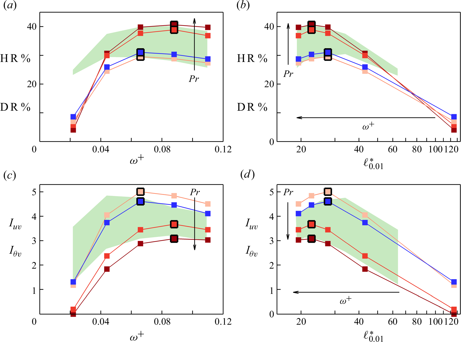
Figure 22 shows that, for $0.066 \le \omega ^+ \le 0.110$
, DR, HR,
$0.066 \le \omega ^+ \le 0.110$
, DR, HR, $I_{u v}$
,
$I_{u v}$
, $I_{\theta v}$
and
$I_{\theta v}$
and $\ell ^*_{0.01}$
for the plane oscillation are close to the values found for the travelling wave. However, as
$\ell ^*_{0.01}$
for the plane oscillation are close to the values found for the travelling wave. However, as $\omega ^+$
decreases to
$\omega ^+$
decreases to $ 0.044$
and then to
$ 0.044$
and then to $0.022$
, significant differences appear. For the plane oscillation, the Stokes layer becomes highly protrusive, reaching up to
$0.022$
, significant differences appear. For the plane oscillation, the Stokes layer becomes highly protrusive, reaching up to $\ell ^*_{0.01} \simeq 120$
at
$\ell ^*_{0.01} \simeq 120$
at $\omega ^+ = 0.022$
. As discussed in § 3.7, such a protrusive Stokes layer loses its efficacy in producing a net attenuation of the near-wall turbulence. As a result,
$\omega ^+ = 0.022$
. As discussed in § 3.7, such a protrusive Stokes layer loses its efficacy in producing a net attenuation of the near-wall turbulence. As a result, $I_{uv}$
and
$I_{uv}$
and $I_{\theta v}$
significantly drop and
$I_{\theta v}$
significantly drop and $\gamma$
rises significantly. Rouhi et al. (Reference Rouhi, Fu, Chandran, Zampiron, Smits and Marusic2023) showed that when
$\gamma$
rises significantly. Rouhi et al. (Reference Rouhi, Fu, Chandran, Zampiron, Smits and Marusic2023) showed that when $\ell ^*_{0.01} \sim \mathcal{O}(10^2)$
, the Stokes layer departs from its laminar-like structure, the mean velocity and temperature profiles become highly disturbed (figure 28
j,k,l), and the predictive relations for DR (3.5a
) and HR (3.5b
) begin to fail. Similarly, we observe that at
$\ell ^*_{0.01} \sim \mathcal{O}(10^2)$
, the Stokes layer departs from its laminar-like structure, the mean velocity and temperature profiles become highly disturbed (figure 28
j,k,l), and the predictive relations for DR (3.5a
) and HR (3.5b
) begin to fail. Similarly, we observe that at $\omega ^+ = 0.022$
the predictive relation for HR (3.5b
) is much less accurate compared with its performance at higher frequencies (figure 21
b).
$\omega ^+ = 0.022$
the predictive relation for HR (3.5b
) is much less accurate compared with its performance at higher frequencies (figure 21
b).
As a final note, it appears that $\gamma$
, a
$\gamma$
, a $Pr$
-independent quantity, increases almost linearly with
$Pr$
-independent quantity, increases almost linearly with $\ell ^*_{0.01}$
and
$\ell ^*_{0.01}$
and $P^*_{{33}_{{max}}}$
, and decreases inversely with increasing
$P^*_{{33}_{{max}}}$
, and decreases inversely with increasing $\omega ^+$
following
$\omega ^+$
following
 \begin{equation} \gamma \simeq 4.2 P^*_{{33}_{{max}}} \simeq 0.008 \ell ^*_{0.01} \simeq {1}/({80\omega ^+}). \end{equation}
This is supported by the results shown in figure 23, where we compile all our data for the travelling wave and the plane oscillation cases (with the exception of the plane oscillation at $\omega ^+ = 0.022$
where the Stokes layer is particularly protrusive). Our present data are at a fixed
$\omega ^+ = 0.022$
where the Stokes layer is particularly protrusive). Our present data are at a fixed $A^+ = 12$
for a plane oscillation (
$A^+ = 12$
for a plane oscillation ( $\kappa ^+_x = 0$
) and a travelling wave (
$\kappa ^+_x = 0$
) and a travelling wave ( $\kappa ^+_x = 0.0014$
). The relation for
$\kappa ^+_x = 0.0014$
). The relation for $\gamma$
(3.10) is expected to also depend on
$\gamma$
(3.10) is expected to also depend on $A^+$
and
$A^+$
and $\kappa ^+_x$
. However, for the upstream travelling wave with
$\kappa ^+_x$
. However, for the upstream travelling wave with $\omega ^+ \gtrsim 0.04$
, we anticipate
$\omega ^+ \gtrsim 0.04$
, we anticipate $\gamma$
to weakly depend on
$\gamma$
to weakly depend on $\kappa ^+_x$
. Our conjecture is partly based on the validity of (3.10) for
$\kappa ^+_x$
. Our conjecture is partly based on the validity of (3.10) for $\kappa ^+_x = 0$
and
$\kappa ^+_x = 0$
and $\kappa ^+_x = 0.0014$
for
$\kappa ^+_x = 0.0014$
for $\omega ^+ \gtrsim 0.04$
. Furthermore,
$\omega ^+ \gtrsim 0.04$
. Furthermore, $\gamma$
relates
$\gamma$
relates $\unicode{x1D6E5} \overline {\Theta }^*_{170}$
to
$\unicode{x1D6E5} \overline {\Theta }^*_{170}$
to $\unicode{x1D6E5} \overline {U}^*_{170}$
, which
$\unicode{x1D6E5} \overline {U}^*_{170}$
, which $\unicode{x1D6E5} \overline {U}^*_{170}$
is seen to weakly depend on
$\unicode{x1D6E5} \overline {U}^*_{170}$
is seen to weakly depend on $\kappa ^+_x$
for the upstream travelling wave with
$\kappa ^+_x$
for the upstream travelling wave with $\omega ^+ \gtrsim 0.04$
(see figure 13 in Gatti & Quadrio Reference Gatti and Quadrio2016), and we anticipate
$\omega ^+ \gtrsim 0.04$
(see figure 13 in Gatti & Quadrio Reference Gatti and Quadrio2016), and we anticipate $\unicode{x1D6E5} \overline {\Theta }^*_{170}$
to behave similarly.
$\unicode{x1D6E5} \overline {\Theta }^*_{170}$
to behave similarly.
Assessment of the relations (3.10) between $\gamma$
,
$\gamma$
, $P^*_{33_{{max}}}$
,
$P^*_{33_{{max}}}$
, $\ell ^*_{0.01}$
and
$\ell ^*_{0.01}$
and $\omega ^+$
for the travelling wave (filled squares) and the plane oscillation (empty circles);
$\omega ^+$
for the travelling wave (filled squares) and the plane oscillation (empty circles); $\omega ^+ = 0.022$
(black),
$\omega ^+ = 0.022$
(black), $0.044$
(blue),
$0.044$
(blue), $0.066$
(red),
$0.066$
(red), $0.088$
(green) and
$0.088$
(green) and $0.110$
(grey).
$0.110$
(grey).
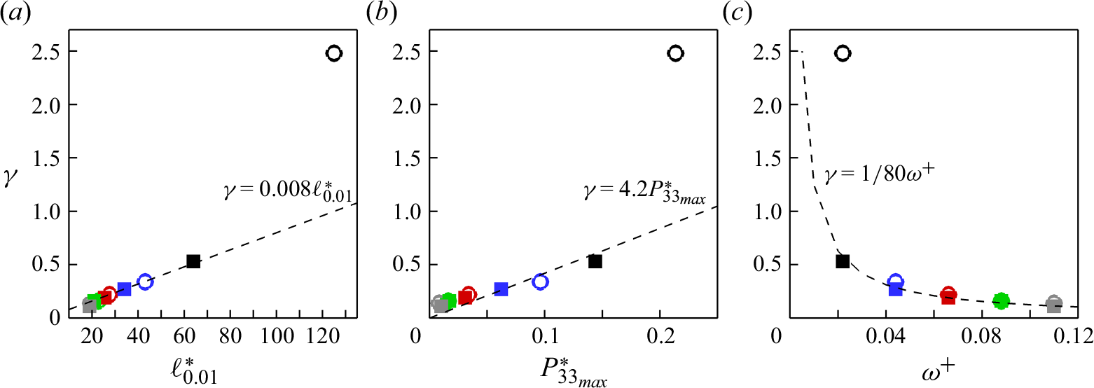
4. Conclusions
Direct numerical simulations of turbulent half-channel flow with forced convection were performed at a friction Reynolds number of 590 for Prandtl numbers of 0.71 (air), 4.0, 7.5 (water) and 20 (molten salt). Spanwise wall forcing was applied either as a plane wall oscillation or a streamwise in-plane travelling wave with wavenumber $\kappa ^+_x = 0.0014$
(
$\kappa ^+_x = 0.0014$
( $\lambda ^+ \simeq 4500$
). For both oscillation mechanisms, we fix the amplitude
$\lambda ^+ \simeq 4500$
). For both oscillation mechanisms, we fix the amplitude $A^+ = 12$
and change the frequency from
$A^+ = 12$
and change the frequency from $\omega ^+ = 0.022$
to
$\omega ^+ = 0.022$
to $0.110$
(upstream travelling waves only).
$0.110$
(upstream travelling waves only).
Schematic illustration of our findings from §§ 3.4to 3.8. The meaning of each sketch is written in the top-left framed area. (a–f) Near-wall illustration of the energetic scales of $uv$
and
$uv$
and $\theta v$
for (a,b) non-actuated cases and (c–f) actuated cases.Panels (a,c,e) correspond to
$\theta v$
for (a,b) non-actuated cases and (c–f) actuated cases.Panels (a,c,e) correspond to $Pr \simeq 1$
, and (b,d,f) correspond to
$Pr \simeq 1$
, and (b,d,f) correspond to $Pr \gt 1$
. For the actuated cases, (c,d) represent
$Pr \gt 1$
. For the actuated cases, (c,d) represent $\omega ^+ \lesssim 0.025$
and (e,f) represent
$\omega ^+ \lesssim 0.025$
and (e,f) represent $\omega ^+ \gt 0.025$
. The Stokes layer production profile is drawn for each actuated case.
$\omega ^+ \gt 0.025$
. The Stokes layer production profile is drawn for each actuated case.
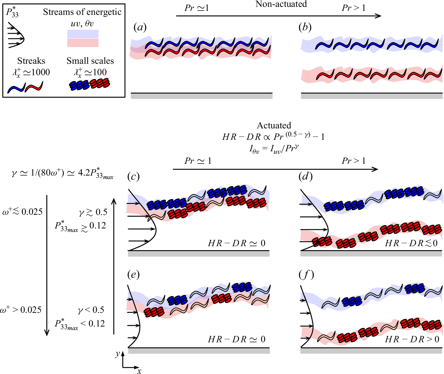
The key finding of the present work is that, for $\omega ^+ \gt 0.022$
and
$\omega ^+ \gt 0.022$
and $Pr \gt 1$
, we achieve
$Pr \gt 1$
, we achieve ${\textrm{HR}} \gt {\textrm{DR}}$
; especially, for
${\textrm{HR}} \gt {\textrm{DR}}$
; especially, for $\omega ^+ \gtrsim 0.066$
and
$\omega ^+ \gtrsim 0.066$
and $Pr \gtrsim 4.0$
, there is a significant disparity between
$Pr \gtrsim 4.0$
, there is a significant disparity between ${\textrm{HR}} \simeq 40\,\%$
and
${\textrm{HR}} \simeq 40\,\%$
and ${\textrm{DR}} \simeq 30\,\%$
. On the other hand, for
${\textrm{DR}} \simeq 30\,\%$
. On the other hand, for $\omega ^+ \le 0.022$
and
$\omega ^+ \le 0.022$
and $Pr \gt 1$
,
$Pr \gt 1$
, ${\textrm{HR}} \lesssim {\textrm{DR}}$
. These results apply to the travelling wave motion and the plane oscillation. To help understand these results, we derived explicit relations between HR and DR and the integrals of the attenuation in the turbulent shear stress (
${\textrm{HR}} \lesssim {\textrm{DR}}$
. These results apply to the travelling wave motion and the plane oscillation. To help understand these results, we derived explicit relations between HR and DR and the integrals of the attenuation in the turbulent shear stress ( $I_{uv}$
) and turbulent temperature flux (
$I_{uv}$
) and turbulent temperature flux ( $I_{\theta v}$
). Figure 24 summarises how
$I_{\theta v}$
). Figure 24 summarises how $I_{uv}$
and
$I_{uv}$
and $I_{\theta v}$
change with
$I_{\theta v}$
change with $Pr$
and
$Pr$
and $\omega ^+$
, and illustrates the underlying physics. For the cases considered here, we find that
$\omega ^+$
, and illustrates the underlying physics. For the cases considered here, we find that $I_{\theta v} \simeq I_{uv}/Pr^{\gamma }$
, where
$I_{\theta v} \simeq I_{uv}/Pr^{\gamma }$
, where $\gamma \simeq 1/(80\omega ^+) \simeq 4.2 P^*_{33_{{max}}}$
is proportional to the Stokes layer production
$\gamma \simeq 1/(80\omega ^+) \simeq 4.2 P^*_{33_{{max}}}$
is proportional to the Stokes layer production $P^*_{33}$
. Therefore, we expect
$P^*_{33}$
. Therefore, we expect $I_{\theta v}$
to fall below
$I_{\theta v}$
to fall below $I_{uv}$
for
$I_{uv}$
for $Pr \gt 1$
and for increasing
$Pr \gt 1$
and for increasing $\gamma$
(decreasing
$\gamma$
(decreasing $\omega ^+$
and increasing
$\omega ^+$
and increasing $P^*_{33}$
). Stokes layer production attenuates the energy of the streak-like scales with
$P^*_{33}$
). Stokes layer production attenuates the energy of the streak-like scales with $\lambda ^+_x \simeq 1000$
(hence, the rise in
$\lambda ^+_x \simeq 1000$
(hence, the rise in $I_{uv}, I_{\theta v}$
), but generates small scales with
$I_{uv}, I_{\theta v}$
), but generates small scales with $\lambda ^+_x \simeq 100$
and amplifies their energy (hence, the drop in
$\lambda ^+_x \simeq 100$
and amplifies their energy (hence, the drop in $I_{uv}, I_{\theta v}$
). At a fixed
$I_{uv}, I_{\theta v}$
). At a fixed $\omega ^+$
(
$\omega ^+$
( $\gamma$
), increasing
$\gamma$
), increasing $Pr$
towards
$Pr$
towards $Pr \gt 1$
, thins the conductive sublayer, and the energetic small scales of
$Pr \gt 1$
, thins the conductive sublayer, and the energetic small scales of $\theta v$
travel closer to the wall, and locally are exposed to a larger Stokes layer production compared with those of
$\theta v$
travel closer to the wall, and locally are exposed to a larger Stokes layer production compared with those of $uv$
. Larger Stokes layer production means larger amplification of energy in the small scales of
$uv$
. Larger Stokes layer production means larger amplification of energy in the small scales of $\theta v$
compared with
$\theta v$
compared with $uv$
, leading to
$uv$
, leading to $I_{\theta v} \lt I_{uv}$
(figure 24
d,f). In other words, for
$I_{\theta v} \lt I_{uv}$
(figure 24
d,f). In other words, for $Pr \gt 1$
, the energy attenuation of
$Pr \gt 1$
, the energy attenuation of $\theta v$
is less than
$\theta v$
is less than $uv$
. Nevertheless, by exploiting
$uv$
. Nevertheless, by exploiting $I_{\theta v} \simeq I_{uv}/Pr^{\gamma }$
, we arrive at
$I_{\theta v} \simeq I_{uv}/Pr^{\gamma }$
, we arrive at ${\textrm{HR}} - {\textrm{DR}} \propto Pr^{(0.5-\gamma )} - 1$
, as HR depends on
${\textrm{HR}} - {\textrm{DR}} \propto Pr^{(0.5-\gamma )} - 1$
, as HR depends on $\unicode{x1D6E5} \overline {\Theta }^* = Pr I_{\theta v} = Pr^{(1-\gamma )} I_{uv}$
, and the non-actuated Stanton number that decays with
$\unicode{x1D6E5} \overline {\Theta }^* = Pr I_{\theta v} = Pr^{(1-\gamma )} I_{uv}$
, and the non-actuated Stanton number that decays with $Pr$
. Therefore, we can achieve
$Pr$
. Therefore, we can achieve ${\textrm{HR}}-{\textrm{DR}} \gt 0$
if
${\textrm{HR}}-{\textrm{DR}} \gt 0$
if $\gamma \lesssim 0.5$
(
$\gamma \lesssim 0.5$
( $\omega ^+ \gtrsim 0.025$
). These findings and the relations between
$\omega ^+ \gtrsim 0.025$
). These findings and the relations between ${\textrm{HR}}-{\textrm{DR}}$
,
${\textrm{HR}}-{\textrm{DR}}$
, $\omega ^+$
,
$\omega ^+$
, $\gamma$
and
$\gamma$
and $P^*_{33_{{max}}}$
agree well with our DNS data for both the travelling wave and the plane oscillation.
$P^*_{33_{{max}}}$
agree well with our DNS data for both the travelling wave and the plane oscillation.
The time scale of the near-wall energetic temperature scales $\mathcal{T}^+_\theta$
was found to be almost insensitive to
$\mathcal{T}^+_\theta$
was found to be almost insensitive to $Pr$
, and it remains close to its counterpart for the velocity scales
$Pr$
, and it remains close to its counterpart for the velocity scales $\mathcal{T}^+_u \simeq 100$
. As a result, for the plane oscillation, the optimal value of
$\mathcal{T}^+_u \simeq 100$
. As a result, for the plane oscillation, the optimal value of $\omega ^+$
for the maximum HRis close to that for the maximum DR, that is,
$\omega ^+$
for the maximum HRis close to that for the maximum DR, that is, $\omega ^+ \simeq 2\pi /100 \simeq 0.066$
. However, for the travelling wave, the optimal frequency for HR changes from
$\omega ^+ \simeq 2\pi /100 \simeq 0.066$
. However, for the travelling wave, the optimal frequency for HR changes from $0.044$
at
$0.044$
at $Pr = 0.71$
to
$Pr = 0.71$
to $0.088$
at
$0.088$
at $Pr = 7.5$
because it depends on the advection speed of the energetic temperature scales. The thinning of the conductive sublayer decreases the advection speed, and so the optimal frequency of actuation increases.
$Pr = 7.5$
because it depends on the advection speed of the energetic temperature scales. The thinning of the conductive sublayer decreases the advection speed, and so the optimal frequency of actuation increases.
From the Prandtl number scaling of the thermal statistics, we derived a predictive model for HR. By knowing $\gamma$
and
$\gamma$
and $I_{uv}$
for a fixed set of actuation parameters
$I_{uv}$
for a fixed set of actuation parameters $(A^+,\kappa ^+_x,\omega ^+)$
at a given Reynolds and Prandtl number, the model predicts HR at other Prandtl and Reynolds numbers. Using this model, we generated a map
$(A^+,\kappa ^+_x,\omega ^+)$
at a given Reynolds and Prandtl number, the model predicts HR at other Prandtl and Reynolds numbers. Using this model, we generated a map ${\textrm{HR}}(Pr, Re_{\tau _0})$
for the optimal case with
${\textrm{HR}}(Pr, Re_{\tau _0})$
for the optimal case with $\omega ^+ = 0.088$
, and found good agreement with the computations for Prandtl numbers up to 7.5. To further evaluate the model, we conducted an extra simulation at
$\omega ^+ = 0.088$
, and found good agreement with the computations for Prandtl numbers up to 7.5. To further evaluate the model, we conducted an extra simulation at $\omega ^+ = 0.088$
and
$\omega ^+ = 0.088$
and $Pr = 20, Re_{\tau _0} = 590$
. Again, good agreement with the model was found (DNS
$Pr = 20, Re_{\tau _0} = 590$
. Again, good agreement with the model was found (DNS ${\textrm{HR}} = 43\,\%, {\textrm{HR}} - {\textrm{DR}} = 13\,\%$
compared with the model
${\textrm{HR}} = 43\,\%, {\textrm{HR}} - {\textrm{DR}} = 13\,\%$
compared with the model ${\textrm{HR}} = 45\,\%, {\textrm{HR}} - {\textrm{DR}} = 14\,\%$
).
${\textrm{HR}} = 45\,\%, {\textrm{HR}} - {\textrm{DR}} = 14\,\%$
).
As an early systematic work on turbulent heat-transfer control by spanwise wall forcing, we focused on $Pr$
and
$Pr$
and $\omega ^+ \gt 0$
, due to their significant effect on HR and
$\omega ^+ \gt 0$
, due to their significant effect on HR and ${\textrm{HR}} - {\textrm{DR}}$
. Our findings are encouraging to pursue this work towards investigating the effects of
${\textrm{HR}} - {\textrm{DR}}$
. Our findings are encouraging to pursue this work towards investigating the effects of $A^+, \kappa ^+_x, Re_{\tau _0}$
and
$A^+, \kappa ^+_x, Re_{\tau _0}$
and $\omega ^+ \lt 0$
(downstream travelling wave). We anticipate that our discoveries could be applied to a wider parameter space. Our conjecture is partly supported by the validity of our findings for both the travelling wave and plane oscillation in the present study. Also, similar findings for DR are shown to be applicable to a wide parameter space of
$\omega ^+ \lt 0$
(downstream travelling wave). We anticipate that our discoveries could be applied to a wider parameter space. Our conjecture is partly supported by the validity of our findings for both the travelling wave and plane oscillation in the present study. Also, similar findings for DR are shown to be applicable to a wide parameter space of $(A^+, \omega ^+, \kappa ^+_x, Re_{\tau _0})$
. The prediction model for DR by Gatti & Quadrio (Reference Gatti and Quadrio2016), the analogue of our model for HR, is shown to agree well with the DNS (Gatti et al. 2024) and LES (Rouhi et al. Reference Rouhi, Fu, Chandran, Zampiron, Smits and Marusic2023) data for
$(A^+, \omega ^+, \kappa ^+_x, Re_{\tau _0})$
. The prediction model for DR by Gatti & Quadrio (Reference Gatti and Quadrio2016), the analogue of our model for HR, is shown to agree well with the DNS (Gatti et al. 2024) and LES (Rouhi et al. Reference Rouhi, Fu, Chandran, Zampiron, Smits and Marusic2023) data for $1000 \lesssim Re_{\tau _0} \lesssim 6000$
over the actuation parameter space where DR significantly changes (
$1000 \lesssim Re_{\tau _0} \lesssim 6000$
over the actuation parameter space where DR significantly changes ( $5 \le A^+ \le 12, 0 \le \kappa ^+_x \le 0.02, -0.2 \le \omega ^+ \le 0.2$
). Also, the findings related to the Stokes layer protrusion and DR are found to be valid over the range of
$5 \le A^+ \le 12, 0 \le \kappa ^+_x \le 0.02, -0.2 \le \omega ^+ \le 0.2$
). Also, the findings related to the Stokes layer protrusion and DR are found to be valid over the range of $\kappa ^+_x$
considered so far. For instance, up to the Stokes layer thickness
$\kappa ^+_x$
considered so far. For instance, up to the Stokes layer thickness $\delta ^*_S \simeq 6$
(protrusion height
$\delta ^*_S \simeq 6$
(protrusion height $\ell ^*_{0.01} \simeq 25$
), there is a linear relation between
$\ell ^*_{0.01} \simeq 25$
), there is a linear relation between ${\textrm{DR}}, \ell ^*_{0.01}$
and
${\textrm{DR}}, \ell ^*_{0.01}$
and $ \delta ^*_S$
, regardless of the value of
$ \delta ^*_S$
, regardless of the value of $\kappa ^+_x$
(Quadrio & Ricco Reference Quadrio and Ricco2011; Rouhi et al. Reference Rouhi, Fu, Chandran, Zampiron, Smits and Marusic2023). This is because the modification of the velocity scales by the Stokes layer is similar between the plane oscillation (Touber & Leschziner Reference Touber and Leschziner2012) and the travelling wave at different values of
$\kappa ^+_x$
(Quadrio & Ricco Reference Quadrio and Ricco2011; Rouhi et al. Reference Rouhi, Fu, Chandran, Zampiron, Smits and Marusic2023). This is because the modification of the velocity scales by the Stokes layer is similar between the plane oscillation (Touber & Leschziner Reference Touber and Leschziner2012) and the travelling wave at different values of $\kappa ^+_x$
(Rouhi et al. Reference Rouhi, Fu, Chandran, Zampiron, Smits and Marusic2023).
$\kappa ^+_x$
(Rouhi et al. Reference Rouhi, Fu, Chandran, Zampiron, Smits and Marusic2023).
Acknowledgements
We acknowledge Dr Daniel Chung for providing his DNS solver. We thank EPSRC for the computational time made available on ARCHER2 via the UK Turbulence Consortium (EP/R029326/1), and the UKRI access to the HPC call 2024. We also acknowledge Intellectual Ventures for providing additional computational time on ARCHER2.
Funding
The research was funded through the Deep Science Fund of Intellectual Ventures.
Declaration of interests
The authors report no conflict of interest.
Appendix A. Validation of the grid and the domain size
The production runs were performed in a reduced-domain half-channel flow ( $L_x \gtrsim 2.7h, L_z \simeq 0.85 h$
) with grid resolution
$L_x \gtrsim 2.7h, L_z \simeq 0.85 h$
) with grid resolution $\unicode{x1D6E5} ^+_x \times \unicode{x1D6E5} ^+_z \simeq 8 \times 4$
; we call this set-up ‘reduced coarse’. To check that this set-up gives accurate
$\unicode{x1D6E5} ^+_x \times \unicode{x1D6E5} ^+_z \simeq 8 \times 4$
; we call this set-up ‘reduced coarse’. To check that this set-up gives accurate ${\textrm{DR}}, {\textrm{HR}}$
and statistics of interest over our parameter space, calculations with a finer grid resolution of
${\textrm{DR}}, {\textrm{HR}}$
and statistics of interest over our parameter space, calculations with a finer grid resolution of $\unicode{x1D6E5} ^+_x \times \unicode{x1D6E5} ^+_z \simeq 4 \times 2$
were conducted in a full domain (
$\unicode{x1D6E5} ^+_x \times \unicode{x1D6E5} ^+_z \simeq 4 \times 2$
were conducted in a full domain ( $L_x \gtrsim 2\pi h, L_z \simeq \pi h$
); we call this set-up ‘full fine’. Two additional set-ups were also used, called ‘full coarse’ (
$L_x \gtrsim 2\pi h, L_z \simeq \pi h$
); we call this set-up ‘full fine’. Two additional set-ups were also used, called ‘full coarse’ ( $L_x \gtrsim 7.6 h, L_z \simeq \pi h, \unicode{x1D6E5} ^+_x \times \unicode{x1D6E5} ^+_z \simeq 8 \times 4$
) and ‘full intermediate’ (
$L_x \gtrsim 7.6 h, L_z \simeq \pi h, \unicode{x1D6E5} ^+_x \times \unicode{x1D6E5} ^+_z \simeq 8 \times 4$
) and ‘full intermediate’ ( $L_x \gtrsim 7.6 h, L_z \simeq \pi h, \unicode{x1D6E5} ^+_x \times \unicode{x1D6E5} ^+_z \simeq 6 \times 3$
). For all simulations,
$L_x \gtrsim 7.6 h, L_z \simeq \pi h, \unicode{x1D6E5} ^+_x \times \unicode{x1D6E5} ^+_z \simeq 6 \times 3$
). For all simulations, $Re_{\tau _0}=590$
and
$Re_{\tau _0}=590$
and $A^+=12$
. For all the reduced-domain cases, we reconstruct the
$A^+=12$
. For all the reduced-domain cases, we reconstruct the $\overline {U}^*$
and
$\overline {U}^*$
and $\overline {\Theta }^*$
profiles beyond
$\overline {\Theta }^*$
profiles beyond $y^*_{{res}} = 170$
, and calculate DR and HR following our approach in § 2.3.
$y^*_{{res}} = 170$
, and calculate DR and HR following our approach in § 2.3.
Validation simulations for the reduced coarse set-up. Non-actuated half-channel flow at $Pr = 7.5$
. Statistics for these cases are shown in figure 25. The reference cases are MKM99 (Moser et al. Reference Moser, Kim and Mansour1999) and AH21 (Alcántara-Á vila & Hoyas Reference Alcántara-Á vila and Hoyas2021).
$Pr = 7.5$
. Statistics for these cases are shown in figure 25. The reference cases are MKM99 (Moser et al. Reference Moser, Kim and Mansour1999) and AH21 (Alcántara-Á vila & Hoyas Reference Alcántara-Á vila and Hoyas2021).
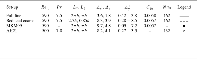
For the non-actuated half-channel flow at $Pr = 7.5$
, table 2 shows that for the full fine and reduced coarse set-ups, the Nusselt numbers
$Pr = 7.5$
, table 2 shows that for the full fine and reduced coarse set-ups, the Nusselt numbers $Nu_0$
are identical and the skin-friction coefficients
$Nu_0$
are identical and the skin-friction coefficients $C_{f_0}$
differ by less than
$C_{f_0}$
differ by less than $2\,\%$
. The profiles of
$2\,\%$
. The profiles of $\overline {U}^+, \overline {\Theta }^+$
, turbulent stresses
$\overline {U}^+, \overline {\Theta }^+$
, turbulent stresses $\overline {u^2}^+, \overline {v^2}^+, \overline {w^2}^+$
and mean square of turbulent temperature
$\overline {u^2}^+, \overline {v^2}^+, \overline {w^2}^+$
and mean square of turbulent temperature $\overline {\theta ^2}^+$
are also in excellent agreement (figure 25). Compared with the reference data, our obtained
$\overline {\theta ^2}^+$
are also in excellent agreement (figure 25). Compared with the reference data, our obtained $C_{f_0}$
from the reduced coarse case is identical to that from Moser et al. (Reference Moser, Kim and Mansour1999) (table 2); similarly, our velocity statistics up to
$C_{f_0}$
from the reduced coarse case is identical to that from Moser et al. (Reference Moser, Kim and Mansour1999) (table 2); similarly, our velocity statistics up to $y^+_{{res}} \simeq 200$
are in excellent agreement (figure 25). In terms of the temperature statistics
$y^+_{{res}} \simeq 200$
are in excellent agreement (figure 25). In terms of the temperature statistics $\overline {\Theta }^+, \overline {\theta ^2}^+$
, the small differences between our results and those from Alcántara-Á vila & Hoyas (Reference Alcántara-Á vila and Hoyas2021) are most likely due to the differences in
$\overline {\Theta }^+, \overline {\theta ^2}^+$
, the small differences between our results and those from Alcántara-Á vila & Hoyas (Reference Alcántara-Á vila and Hoyas2021) are most likely due to the differences in $Re_{\tau _0}$
and
$Re_{\tau _0}$
and $Pr$
(590 compared with 500 and 7.5 compared with 7).
$Pr$
(590 compared with 500 and 7.5 compared with 7).
Comparing the results for the three set-ups given in table 2. (a) Mean velocity profiles $\overline {U}^+$
. (b) Turbulent stresses
$\overline {U}^+$
. (b) Turbulent stresses $\overline {u^2}^+, \overline {v^2}^+, \overline {w^2}^+$
. (c) Mean temperature profiles
$\overline {u^2}^+, \overline {v^2}^+, \overline {w^2}^+$
. (c) Mean temperature profiles $\overline {\Theta }^+$
. (d) Mean square of turbulent temperature
$\overline {\Theta }^+$
. (d) Mean square of turbulent temperature $\overline { \theta ^2 }^+$
. Solid grey line, ‘full fine’ set-up. Dashed line: ‘reduced coarse’ set-up. The solid black line in (a,c)is the reconstructed profile for
$\overline { \theta ^2 }^+$
. Solid grey line, ‘full fine’ set-up. Dashed line: ‘reduced coarse’ set-up. The solid black line in (a,c)is the reconstructed profile for $y^+ \ge 200$
, as in § 2.3. Square symbols: DNS of Moser et al. (Reference Moser, Kim and Mansour1999). Circle symbols: DNS of Alcántara-Á vila & Hoyas (Reference Alcántara-Á vila and Hoyas2021).
$y^+ \ge 200$
, as in § 2.3. Square symbols: DNS of Moser et al. (Reference Moser, Kim and Mansour1999). Circle symbols: DNS of Alcántara-Á vila & Hoyas (Reference Alcántara-Á vila and Hoyas2021).
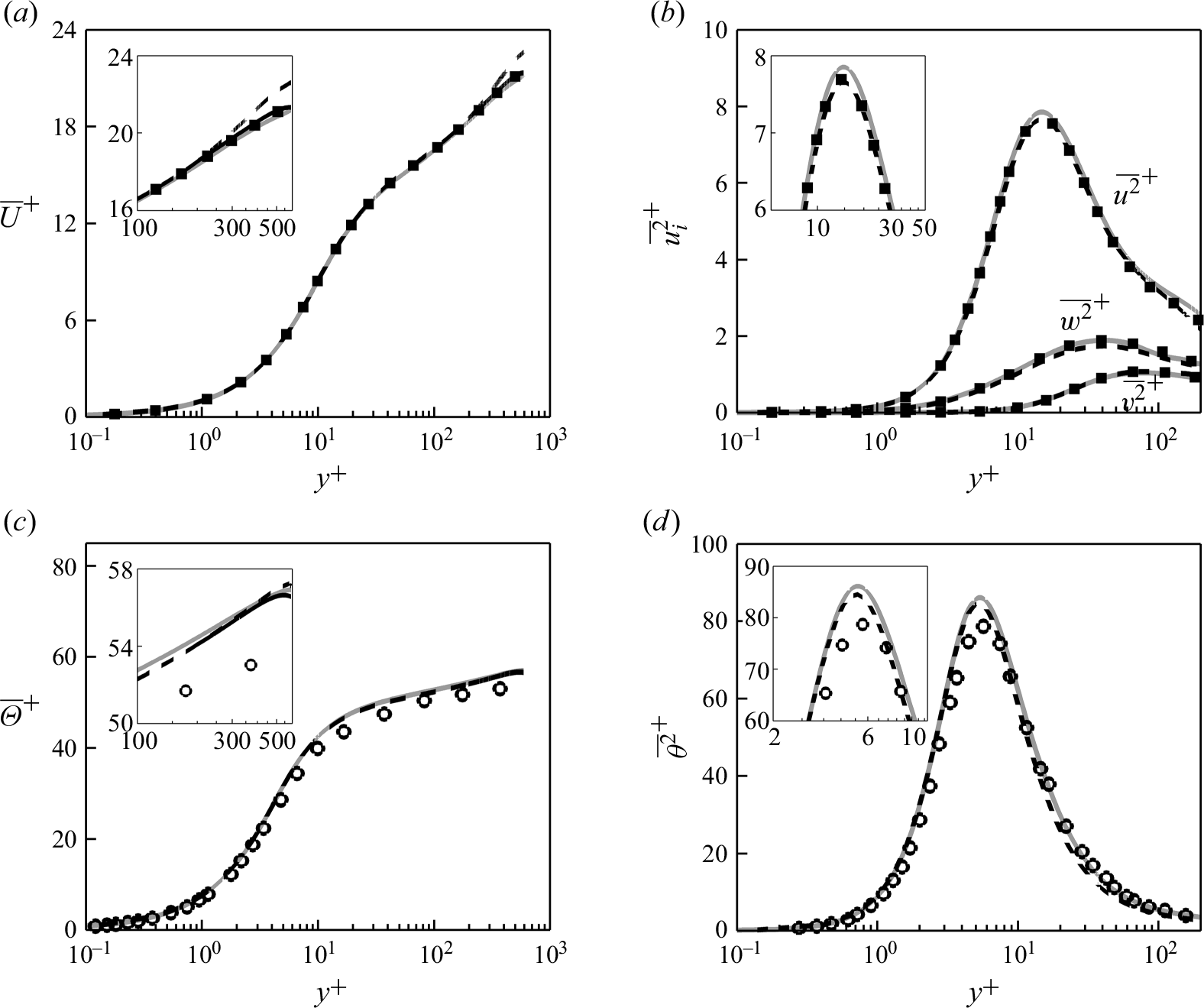
Validation simulations for grid and domain size.
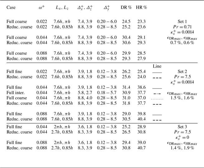
For the actuated half-channel flow cases at $Pr=0.71$
and
$Pr=0.71$
and $7.5$
, table 3 lists three sets of validation cases. For set 1, we compare the ‘reduced coarse’ set-up with the ‘full coarse’ set-up because the grid resolution of
$7.5$
, table 3 lists three sets of validation cases. For set 1, we compare the ‘reduced coarse’ set-up with the ‘full coarse’ set-up because the grid resolution of $\unicode{x1D6E5} ^+_x \times \unicode{x1D6E5} ^+_z \simeq 8 \times 4$
is fine enough at this
$\unicode{x1D6E5} ^+_x \times \unicode{x1D6E5} ^+_z \simeq 8 \times 4$
is fine enough at this $Pr$
(Pirozzoli et al. Reference Pirozzoli, Bernardini and Orlandi2016; Alcántara-Á vila et al. Reference Alcántara-Á vila and Pérez-Quiles2018, Reference Alcántara-Á vila and Pérez-Quiles2021; Alcántara-Á vila & Hoyas Reference Alcántara-Á vila and Hoyas2021). Sets 1 and 2 are travelling wave cases, and set 3 is for the plane oscillation case. For each set, we see that reducing the domain size and coarsening the grid from the full fine set-up to the reduced coarse set-up changes DR and HR by a maximum of
$Pr$
(Pirozzoli et al. Reference Pirozzoli, Bernardini and Orlandi2016; Alcántara-Á vila et al. Reference Alcántara-Á vila and Pérez-Quiles2018, Reference Alcántara-Á vila and Pérez-Quiles2021; Alcántara-Á vila & Hoyas Reference Alcántara-Á vila and Hoyas2021). Sets 1 and 2 are travelling wave cases, and set 3 is for the plane oscillation case. For each set, we see that reducing the domain size and coarsening the grid from the full fine set-up to the reduced coarse set-up changes DR and HR by a maximum of $1.5\,\%$
and
$1.5\,\%$
and $1.9\,\%$
, respectively.
$1.9\,\%$
, respectively.
Set 2 contains the most challenging cases over the range $0.71 \le Pr \le 7.5$
in terms of their grid resolution requirement. In figure 26 we compare the mean velocity
$0.71 \le Pr \le 7.5$
in terms of their grid resolution requirement. In figure 26 we compare the mean velocity $\overline {U}^*$
and the mean temperature
$\overline {U}^*$
and the mean temperature $\overline {\Theta }^*$
profiles for
$\overline {\Theta }^*$
profiles for $Pr = 7.5$
. In terms of the
$Pr = 7.5$
. In terms of the $\overline {U}^*$
profiles, the reduced coarse set-up is almost identical to the full fine set-up up to
$\overline {U}^*$
profiles, the reduced coarse set-up is almost identical to the full fine set-up up to $y^*_{{res}} \simeq 170$
. Beyond
$y^*_{{res}} \simeq 170$
. Beyond $y^*_{{res}}$
, the reconstructed
$y^*_{{res}}$
, the reconstructed $\overline {U}^*$
profiles for the reduced coarse set-up agree well with the full fine set-up. In terms of the
$\overline {U}^*$
profiles for the reduced coarse set-up agree well with the full fine set-up. In terms of the $\overline {\Theta }^*$
profiles, excellent agreement is obtained between the full fine set-up and the reduced coarse set-up at
$\overline {\Theta }^*$
profiles, excellent agreement is obtained between the full fine set-up and the reduced coarse set-up at $\omega ^+ = 0.022$
and
$\omega ^+ = 0.022$
and $0.088$
(figure 26
a,c). At
$0.088$
(figure 26
a,c). At $\omega ^+ = 0.044$
, there is some sensitivity to the grid, where at
$\omega ^+ = 0.044$
, there is some sensitivity to the grid, where at $y^* = 200$
,
$y^* = 200$
, $\overline {\Theta }^* = 74.3$
for the full fine set-up and 73.0 for the reduced coarse set-up. This difference (1.3 units) is small relative to the temperature difference
$\overline {\Theta }^* = 74.3$
for the full fine set-up and 73.0 for the reduced coarse set-up. This difference (1.3 units) is small relative to the temperature difference $\unicode{x1D6E5} \overline {\Theta }^*_{200} \simeq 19.0$
between the actuated and non-actuated profiles. In figure 27 we assess the accuracy of the reduced coarse set-up in resolving
$\unicode{x1D6E5} \overline {\Theta }^*_{200} \simeq 19.0$
between the actuated and non-actuated profiles. In figure 27 we assess the accuracy of the reduced coarse set-up in resolving $\overline {u^2}^*$
and
$\overline {u^2}^*$
and $\overline {\theta ^2}^*$
, as well as their pre-multiplied spectrograms
$\overline {\theta ^2}^*$
, as well as their pre-multiplied spectrograms $k^*_x \phi ^*_{uu}, k^*_z \phi ^*_{uu}, k^*_x \phi ^*_{\theta \theta }, k^*_z \phi ^*_{\theta \theta }$
at
$k^*_x \phi ^*_{uu}, k^*_z \phi ^*_{uu}, k^*_x \phi ^*_{\theta \theta }, k^*_z \phi ^*_{\theta \theta }$
at $\omega ^+ = 0.044$
. The reduced coarse set-up results agree well with the full fine set-up results, especially in matching the energetic peaks in the spectrograms in terms of magnitude, location
$\omega ^+ = 0.044$
. The reduced coarse set-up results agree well with the full fine set-up results, especially in matching the energetic peaks in the spectrograms in terms of magnitude, location $y^*$
and length scales
$y^*$
and length scales $\lambda ^*_x, \lambda ^*_z$
.
$\lambda ^*_x, \lambda ^*_z$
.
Comparison of the mean velocity (a,b,c) and the mean temperature (d,e,f) profiles for the travelling wave at $Pr = 7.5$
(set 2, table 3). Results are shown for (a,d)
$Pr = 7.5$
(set 2, table 3). Results are shown for (a,d) $\omega ^+ = 0.022$
, (b,e)
$\omega ^+ = 0.022$
, (b,e) $\omega ^+ = 0.044$
and (c,f)
$\omega ^+ = 0.044$
and (c,f) $\omega ^+ = 0.088$
. Solid grey line: ‘full fine’ case. Dashed-dotted line: ‘full inter.’ case. Dotted line: full coarse case. Dashed line:‘reduc. coarse’ case. Solid blue and red linesare the reconstructed profiles for
$\omega ^+ = 0.088$
. Solid grey line: ‘full fine’ case. Dashed-dotted line: ‘full inter.’ case. Dotted line: full coarse case. Dashed line:‘reduc. coarse’ case. Solid blue and red linesare the reconstructed profiles for $y^* \ge 170$
, as in § 2.3. Solid black line: non-actuated ‘full fine’ case.
$y^* \ge 170$
, as in § 2.3. Solid black line: non-actuated ‘full fine’ case.
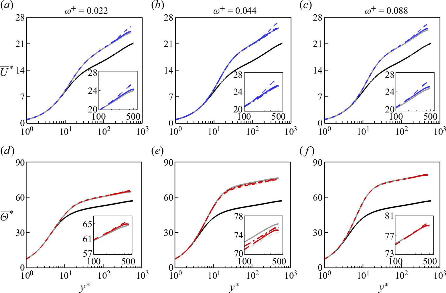
Comparison of (a) streamwise turbulent stress $\overline {u^2}^*$
and (d) mean square of turbulent temperature
$\overline {u^2}^*$
and (d) mean square of turbulent temperature $\overline {\theta ^2}^*$
, as well as their pre-multiplied spectrograms
$\overline {\theta ^2}^*$
, as well as their pre-multiplied spectrograms $k^*_x \phi ^*_{uu}, k^*_z \phi ^*_{uu}, k^*_x \phi ^*_{\theta \theta }, k^*_z \phi ^*_{\theta \theta }$
(b,c,e,f) for the travelling wave at
$k^*_x \phi ^*_{uu}, k^*_z \phi ^*_{uu}, k^*_x \phi ^*_{\theta \theta }, k^*_z \phi ^*_{\theta \theta }$
(b,c,e,f) for the travelling wave at $Pr = 7.5$
,
$Pr = 7.5$
, $\omega ^+=0.044$
(set 2, table 3). Solid grey line and grey-scale contour field: ‘full fine’ case. Dotted line and dotted contour lines: ‘full coarse’ case. Dashed line and dashed contour lines:‘reduc. coarse’ case.
$\omega ^+=0.044$
(set 2, table 3). Solid grey line and grey-scale contour field: ‘full fine’ case. Dotted line and dotted contour lines: ‘full coarse’ case. Dashed line and dashed contour lines:‘reduc. coarse’ case.
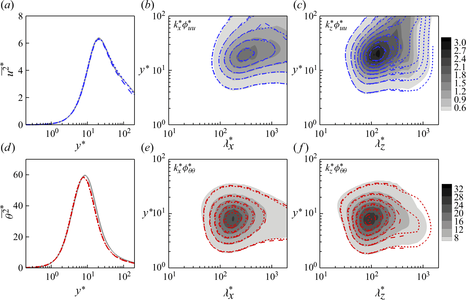
Table 4 summarises our validation study at $Pr = 20.0$
(table 1). For the non-actuated case (table 4),
$Pr = 20.0$
(table 1). For the non-actuated case (table 4), $C_{f_0}$
and
$C_{f_0}$
and $C_{h_0}$
from the coarse grid results differ from the intermediate grid results by a maximum of
$C_{h_0}$
from the coarse grid results differ from the intermediate grid results by a maximum of $0.5\,\%$
, and for the travelling wave case, DR and HR differ by
$0.5\,\%$
, and for the travelling wave case, DR and HR differ by $\lt 1\,\%$
.
$\lt 1\,\%$
.
Based on these results, we conclude that ${\textrm{DR}}, {\textrm{HR}}$
and the statistics of interest can be accurately computed using the reduced coarse set-up with the grid resolution of
${\textrm{DR}}, {\textrm{HR}}$
and the statistics of interest can be accurately computed using the reduced coarse set-up with the grid resolution of $\unicode{x1D6E5} ^+_x \times \unicode{x1D6E5} ^+_z \simeq 8 \times 4$
, and the domain size of
$\unicode{x1D6E5} ^+_x \times \unicode{x1D6E5} ^+_z \simeq 8 \times 4$
, and the domain size of $L_x \times L_z \simeq 7.6 h \times 0.85 h$
for the travelling wave case (
$L_x \times L_z \simeq 7.6 h \times 0.85 h$
for the travelling wave case ( $\kappa ^+_x = 0.0014$
), and the domain size of
$\kappa ^+_x = 0.0014$
), and the domain size of $L_x \times L_z \simeq 2.7 h \times 0.85 h$
for the plane oscillation case (
$L_x \times L_z \simeq 2.7 h \times 0.85 h$
for the plane oscillation case ( $\kappa ^+_x = 0$
). These grid and domain size prescriptions were used for our production calculations (table 1).
$\kappa ^+_x = 0$
). These grid and domain size prescriptions were used for our production calculations (table 1).
Appendix B. Relation between HR and temperature difference
The mean velocity $\overline {U}^*$
and temperature
$\overline {U}^*$
and temperature $\overline {\Theta }^*$
profiles in the log region and beyond can be expressed based on the following semi-empirical wall-wake relations (Rouhi et al. Reference Rouhi, Endrikat, Modesti, Sandberg, Oda, Tanimoto, Hutchins and Chung2022):
$\overline {\Theta }^*$
profiles in the log region and beyond can be expressed based on the following semi-empirical wall-wake relations (Rouhi et al. Reference Rouhi, Endrikat, Modesti, Sandberg, Oda, Tanimoto, Hutchins and Chung2022):
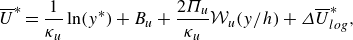 \begin{align} \overline {U}^* &= \frac {1}{\kappa _u} \ln (y^*) + B_u + \frac {2\Pi _u}{\kappa _u}\mathcal{W}_u(y/h) + \unicode{x1D6E5} \overline {U}^*_{{log}}, \end{align}
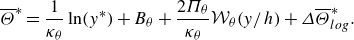 \begin{align} \overline {\Theta }^* &= \frac {1}{\kappa _\theta } \ln (y^*) + B_\theta + \frac {2\Pi _\theta }{\kappa _\theta }\mathcal{W}_\theta (y/h) + \unicode{x1D6E5} \overline {\Theta }^*_{{log}}. \\[6pt] \nonumber \end{align}
Here $\kappa _u, \kappa _\theta$
and
$\kappa _u, \kappa _\theta$
and $B_u$
are constants, but the offset
$B_u$
are constants, but the offset $B_\theta$
depends on
$B_\theta$
depends on $Pr$
(Kader & Yaglom Reference Kader and Yaglom1972; Kader Reference Kader1981). The wake profiles
$Pr$
(Kader & Yaglom Reference Kader and Yaglom1972; Kader Reference Kader1981). The wake profiles $(2\Pi _u/\kappa _u)\mathcal{W}_u(y/h)$
and
$(2\Pi _u/\kappa _u)\mathcal{W}_u(y/h)$
and $ (2\Pi _\theta /\kappa _\theta )\mathcal{W}_\theta (y/h)$
depend on the flow configuration, e.g. channel, pipe or boundary layer (Pope Reference Pope2000; Nagib & Chauhan Reference Nagib and Chauhan2008). The log-law shifts,
$ (2\Pi _\theta /\kappa _\theta )\mathcal{W}_\theta (y/h)$
depend on the flow configuration, e.g. channel, pipe or boundary layer (Pope Reference Pope2000; Nagib & Chauhan Reference Nagib and Chauhan2008). The log-law shifts, $\unicode{x1D6E5} \overline {U}^*_{{log}}$
and
$\unicode{x1D6E5} \overline {U}^*_{{log}}$
and $\unicode{x1D6E5} \overline {\Theta }^*_{{log}}$
, are non-zero for the actuated cases. These log-law shifts are evaluated at
$\unicode{x1D6E5} \overline {\Theta }^*_{{log}}$
, are non-zero for the actuated cases. These log-law shifts are evaluated at $y^* = 170$
, where
$y^* = 170$
, where $\unicode{x1D6E5} \overline {U}^*$
and
$\unicode{x1D6E5} \overline {U}^*$
and $\unicode{x1D6E5} \overline {\Theta }^*$
approximately reach their asymptotic values (figures 4 and 8). For fixed operating parameters (
$\unicode{x1D6E5} \overline {\Theta }^*$
approximately reach their asymptotic values (figures 4 and 8). For fixed operating parameters ( $A^+, \kappa ^+_x, \omega ^+$
),
$A^+, \kappa ^+_x, \omega ^+$
), $\unicode{x1D6E5} \overline {U}^*_{{log}}$
is constant for the upstream travelling wave (Hurst et al. Reference Hurst, Yang and Chung2014; Gatti & Quadrio Reference Gatti and Quadrio2016; Rouhi et al. Reference Rouhi, Fu, Chandran, Zampiron, Smits and Marusic2023). However,
$\unicode{x1D6E5} \overline {U}^*_{{log}}$
is constant for the upstream travelling wave (Hurst et al. Reference Hurst, Yang and Chung2014; Gatti & Quadrio Reference Gatti and Quadrio2016; Rouhi et al. Reference Rouhi, Fu, Chandran, Zampiron, Smits and Marusic2023). However, $\unicode{x1D6E5} \overline {\Theta }^*_{{log}}$
strongly depends on
$\unicode{x1D6E5} \overline {\Theta }^*_{{log}}$
strongly depends on $Pr$
(figure 8
k,l). We set the constants
$Pr$
(figure 8
k,l). We set the constants $\kappa _u = 0.4$
,
$\kappa _u = 0.4$
, $\kappa _\theta = 0.46$
and
$\kappa _\theta = 0.46$
and $B_u = 5.2$
following Pirozzoli et al. (Reference Pirozzoli, Bernardini and Orlandi2016) and Rouhi et al. (Reference Rouhi, Endrikat, Modesti, Sandberg, Oda, Tanimoto, Hutchins and Chung2022), and obtain the offset
$B_u = 5.2$
following Pirozzoli et al. (Reference Pirozzoli, Bernardini and Orlandi2016) and Rouhi et al. (Reference Rouhi, Endrikat, Modesti, Sandberg, Oda, Tanimoto, Hutchins and Chung2022), and obtain the offset $B_\theta (Pr) = 12.5 Pr^{2/3} + 2.12 \ln Pr - 5.3$
following Kader & Yaglom (Reference Kader and Yaglom1972), which is reported to be accurate for
$B_\theta (Pr) = 12.5 Pr^{2/3} + 2.12 \ln Pr - 5.3$
following Kader & Yaglom (Reference Kader and Yaglom1972), which is reported to be accurate for $Pr \gtrsim 0.7$
. The suitability of these choices is confirmed in § 2.3 and Appendix A.
$Pr \gtrsim 0.7$
. The suitability of these choices is confirmed in § 2.3 and Appendix A.
The bulk velocity $U^*_b$
and bulk temperature
$U^*_b$
and bulk temperature $\Theta ^*_b$
are found by integrating (C1a
) and (C1b
), so that
$\Theta ^*_b$
are found by integrating (C1a
) and (C1b
), so that
 \begin{align} U^*_b &= \frac {1}{\kappa _u} \ln (Re_\tau ) - \frac {1}{\kappa _u} + B_u + \frac {2\Pi _u}{\kappa _u}\int _0^h\mathcal{W}_u(y/h){\mathrm d}y + \unicode{x1D6E5} \overline {U}^*_{{log}}, \end{align}
 \begin{align} \Theta ^*_b &= \frac {1}{\kappa _\theta } \ln (Re_\tau ) - \frac {1}{\kappa _\theta } + B_\theta + \frac {2\Pi _\theta }{\kappa _\theta }\int _0^h\mathcal{W}_\theta (y/h){\mathrm d}y +\unicode{x1D6E5} \overline {\Theta }^*_{{log}}. \end{align}
By subtracting the non-actuated $U^*_{b_0}$
and
$U^*_{b_0}$
and $\Theta ^*_{b_0}$
from their actuated counterparts
$\Theta ^*_{b_0}$
from their actuated counterparts $U^*_b$
and
$U^*_b$
and $\Theta ^*_b$
, and by assuming that the wake profiles are not influenced by the wall oscillation, we obtain
$\Theta ^*_b$
, and by assuming that the wake profiles are not influenced by the wall oscillation, we obtain
 \begin{align} U^*_b - U^*_{b_0} = \frac {1}{\kappa _u} \ln \left ( \frac {Re_\tau }{Re_{\tau _0}} \right ) + \unicode{x1D6E5} \overline {U}^*_{{log}}, \qquad \Theta ^*_b - \Theta ^*_{b_0} = \frac {1}{\kappa _\theta } \ln \left ( \frac {Re_\tau }{Re_{\tau _0}} \right ) + \unicode{x1D6E5} \overline {\Theta }^*_{{log}}. \end{align}
When $Re_\tau$
is matched between the actuated and non-actuated cases (
$Re_\tau$
is matched between the actuated and non-actuated cases ( $Re_\tau = Re_{\tau _0}$
), the first term on the right-hand side of (C3) disappears. However, when the bulk Reynolds number
$Re_\tau = Re_{\tau _0}$
), the first term on the right-hand side of (C3) disappears. However, when the bulk Reynolds number $Re_b$
is matched, as in our work, this term is retained because
$Re_b$
is matched, as in our work, this term is retained because $Re_\tau \ne Re_{\tau _0}$
. By using (C3) and the relations
$Re_\tau \ne Re_{\tau _0}$
. By using (C3) and the relations $C_f = 2/{U^*_b}^2, \ C_h = 1/(U^*_b \Theta ^*_b), \ C_f/C_{f_0} = R_f = 1-{\textrm{DR}}$
and
$C_f = 2/{U^*_b}^2, \ C_h = 1/(U^*_b \Theta ^*_b), \ C_f/C_{f_0} = R_f = 1-{\textrm{DR}}$
and $ C_h/C_{h_0} = R_h = 1-{\textrm{HR}}$
, we can relate
$ C_h/C_{h_0} = R_h = 1-{\textrm{HR}}$
, we can relate $\unicode{x1D6E5} \overline {U}^*_{{log}}$
and
$\unicode{x1D6E5} \overline {U}^*_{{log}}$
and $\unicode{x1D6E5} \overline {\Theta }^*_{{log}}$
to
$\unicode{x1D6E5} \overline {\Theta }^*_{{log}}$
to $R_f$
and
$R_f$
and $R_h$
according to
$R_h$
according to
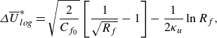 \begin{align} \unicode{x1D6E5} \overline {U}^*_{{log}} &= \sqrt {\frac {2}{C_{f_0}}}\left [ \frac {1}{\sqrt {R_f}} - 1 \right ] - \frac {1}{2\kappa _u}\ln R_f, \end{align}
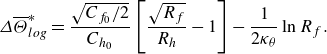 \begin{align} \unicode{x1D6E5} \overline {\Theta }^*_{{log}} &= \frac {\sqrt {C_{f_0}/2}}{C_{h_0}}\left [ \frac {\sqrt {R_f}}{R_h} - 1 \right ] - \frac {1}{2\kappa _\theta }\ln R_f . \end{align}
Validation cases at $Re_{\tau _0} = 590$
and
$Re_{\tau _0} = 590$
and $Pr = 20.0$
.
$Pr = 20.0$
.
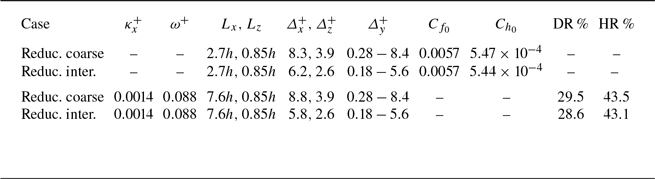
Equation (C4a ) was first derived by Gatti & Quadrio (Reference Gatti and Quadrio2016) (their equation 4.7). Equation (C4b ) is new.
Appendix C. Statistics for the plane oscillation
Same plots as in figure 8, but for the plane oscillation case with $A^+ = 12$
.
$A^+ = 12$
.
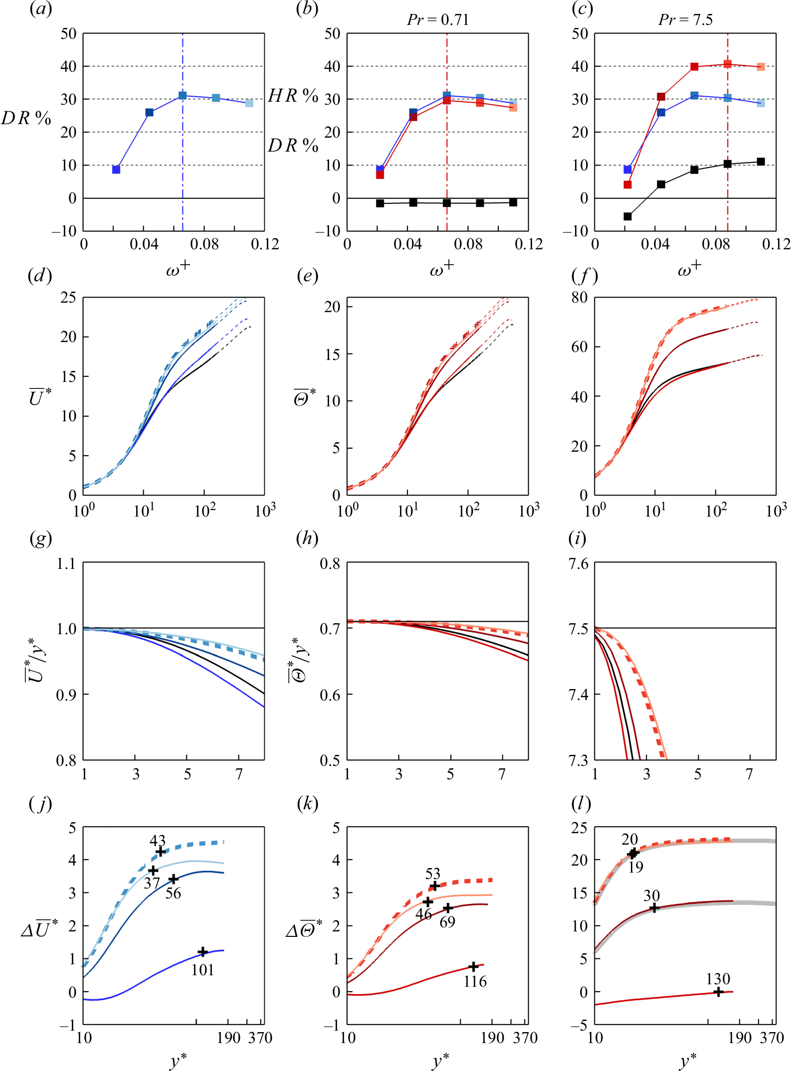
Same plots as in figure 9, but for the plane oscillation case with $A^+ = 12$
.
$A^+ = 12$
.
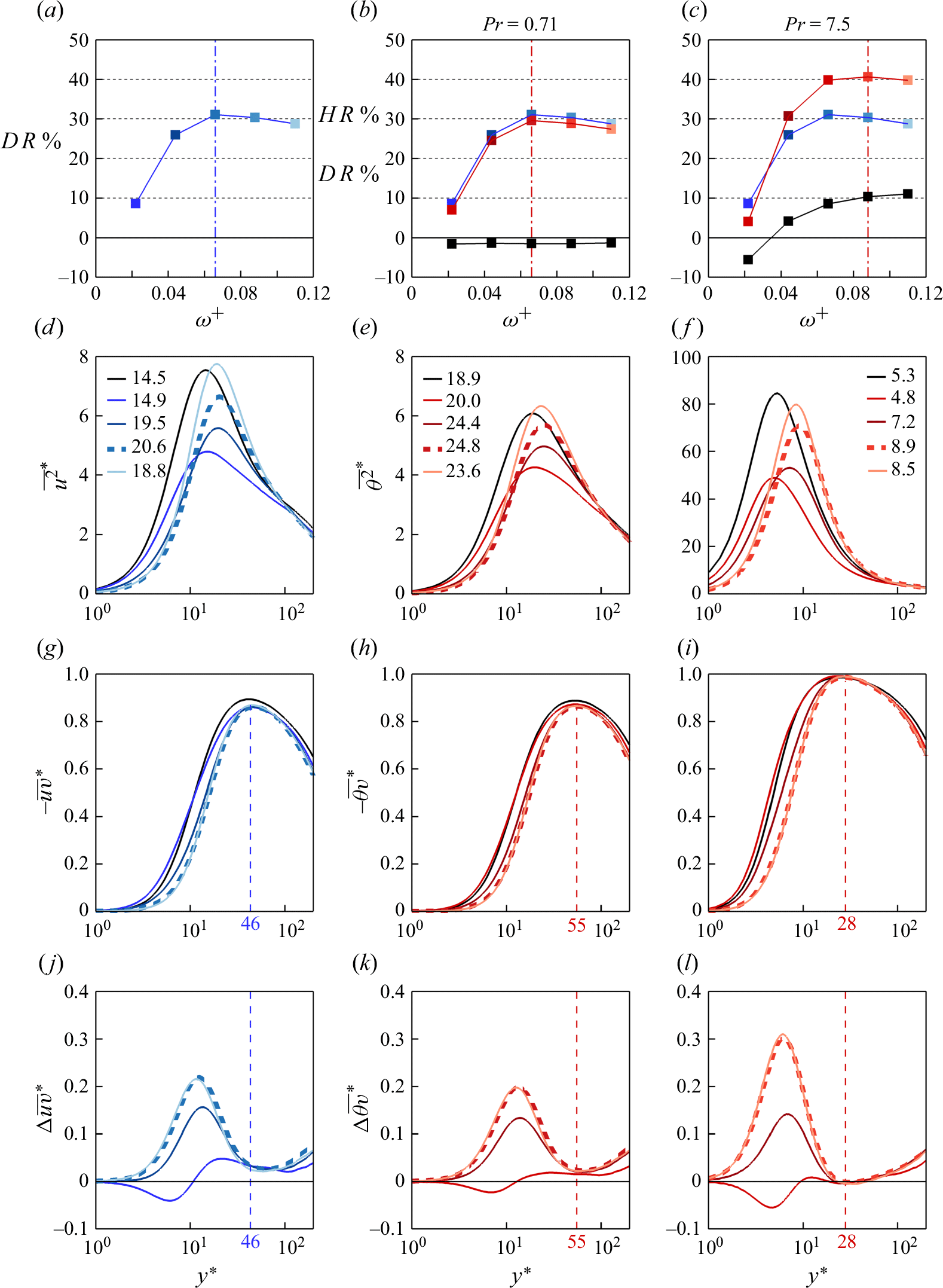
See figures 28 and 29.


 Open access