


1. Introduction
The study of fluid dynamics is fundamental to understanding a wide range of natural and engineered systems, from atmospheric phenomena to industrial processes. Central to this field is the propagation of fluctuations in fluids, which underpins our understanding of acoustics, turbulence and flow stability (Ren, Fu & Pecnik Reference Ren, Fu and Pecnik2019). Traditionally, research on linear waves in fluids has focused on ideal gases, where the assumptions of negligible intermolecular forces and molecular volumes simplify the governing equations (Poling, Prausnitz & O’Connell Reference Poling, Prausnitz and O’Connell2001). However, many real-world fluids deviate from these idealisations, necessitating a more general approach.
Non-ideal fluids, characterised by significant intermolecular interactions and complex equations of state (EOSs), present a rich and challenging area of study (Menikoff & Plohr Reference Menikoff and Plohr1989; Kluwick Reference Kluwick2018; Guardone et al. Reference Guardone, Colonna, Pini and Spinelli2024). These fluids are prevalent in various industrial applications, including heat exchangers (Romei et al. Reference Romei, Vimercati, Persico and Guardone2020), petroleum engineering, chemical processing, aerospace engineering (Cinnella & Congedo Reference Cinnella and Congedo2007) and defence applications. In heat exchanger systems (Nieuwenhuyse, Lecompte & Paepe Reference Van Nieuwenhuyse, Lecompte and De Paepe2023), working fluids sometimes operate under conditions where intermolecular forces significantly impact efficiency and performance. In petroleum engineering (De Hemptinne & Béhar Reference De Hemptinne and Béhar2006), hydrocarbon extraction and processing involve fluids that exhibit non-ideal behaviour due to high pressures and temperatures – e.g. the flash-gas phenomenon – affecting the flow dynamics in pipelines and reservoirs. Similarly, in chemical processing (Brunner Reference Brunner2010), reactor design and operation require a deep understanding of non-ideal fluid behaviour to optimise reaction conditions and ensure safety. In aerospace engineering, high-speed flows and combustion processes under high-pressure conditions necessitate accounting for non-ideal effects to accurately model and predict propulsion performance (Jofre & Urzay Reference Jofre and Urzay2021). Furthermore, in explosion dynamics, overpressure can be sufficiently large for the surrounding solid materials (Powers Reference Powers2004; Saurel et al. Reference Saurel, Métayer, Massoni and Gavrilyuk2007) or the undetonated condensed explosive itself (Lozano, Cawkwell & Aslam Reference Lozano, Cawkwell and Aslam2023) to be effectively modelled in hydrocodes as fluids with highly non-ideal EOSs (Chiapolino & Saurel Reference Chiapolino and Saurel2025). Non-ideal EOSs are also often best expressed explicitly as functions of temperature, which introduces additional challenges to numerical methods (Sirianni et al. Reference Sirianni, Guardone, Re and Abgrall2024; Vienne, Giauque & Lévêque Reference Vienne, Giauque and Lévêque2024; Yan et al. Reference Yan, Gori, Zocca and Guardone2025). Understanding linear wave propagation in non-ideal fluids – i.e. with non-ideal EOSs – is therefore crucial for optimising these processes and predicting fluid behaviour under diverse conditions.
Linear waves in ideal gases have been extensively studied (see e.g. Kirchhoff Reference Kirchhoff1868; Kovásznay Reference Kovásznay1953; Chu & Kovásznay Reference Chu and Kovásznay1958; Chu Reference Chu1965; Fletcher Reference Fletcher1974; Stokes Reference Stokes2009; Benjelloun & Ghidaglia Reference Benjelloun and Ghidaglia2020). Recently, Alferez & Touber (Reference Alferez and Touber2017), Touber & Alferez (Reference Touber and Alferez2019) derived the linear wave dynamics in inviscid, non-conducting and non-ideal fluids. This paper has two main objectives. First, it extends classical linear wave theory to encompass viscous heat-conducting non-ideal compressible fluids, i.e. fluids with an arbitrary EOS. Second, it re-examines the problem of dispersion and attenuation of linear fluctuations in fluids using modern numerical tools, which enable a much more efficient exploration of dispersion relations in fluids. By leveraging the Navier–Stokes–Fourier model, closed with an arbitrary EOS, this study integrates non-ideal effects into the ideal gas framework proposed by Kovásznay (Reference Kovásznay1953), Chu & Kovásznay (Reference Chu and Kovásznay1958) and Chu (Reference Chu1965). It elucidates wave propagation and attenuation in arbitrary non-ideal fluids. This research advances theoretical fluid dynamics while also providing practical insights applicable to a wide range of industrial and research contexts, enabling more accurate modelling and simulation of complex fluid systems.
The article is structured as follows. Section 2 presents the fundamental equations of continuum fluid physics and thermodynamics used in this study. In § 3, these equations are linearised around a stationary and homogeneous base flow. A Helmholtz–Hodge decomposition of velocity simplifies the problem, and plane wave solutions and relevant non-dimensional numbers are introduced and discussed. Based on the linearised equations obtained in § 3, two families of linear waves are identified as solutions of the Navier–Stokes–Fourier model. Their dispersion relations – linking angular frequency to the wave vector of a plane wave – are analysed. The first family, referred to as hydrodynamic (or vorticity) modes, is examined in § 4. The second family, termed thermodynamic (or pressure-entropy) modes, is analysed in § 5. In § 6, a library is used to demonstrate how the general formalism introduced in previous sections can be applied to very different fluids under very different thermodynamic conditions. Finally, conclusions and final remarks are presented in § 7.
2. Thermo-hydrodynamics of non-ideal compressible fluids
Fluids in the continuous regime have diverse properties that can be observed macroscopically. If the influence of body forces and heat injection are neglected, the density $\rho$
, velocity
$\rho$
, velocity $\boldsymbol{u}$
and specific total energy
$\boldsymbol{u}$
and specific total energy $E$
of an arbitrary fluid are governed by the Navier–Stokes–Fourier model (Liepmann & Roshko Reference Liepmann and Roshko2001)
$E$
of an arbitrary fluid are governed by the Navier–Stokes–Fourier model (Liepmann & Roshko Reference Liepmann and Roshko2001)
 \begin{align}&\qquad\qquad\,\, \displaystyle \frac {\partial \rho }{\partial t} + \boldsymbol{\nabla }\boldsymbol{\cdot }\left (\rho \boldsymbol{u}\right ) = 0, \end{align}
 \begin{align}&\quad\,\, \displaystyle \frac {\partial \rho \boldsymbol{u}}{\partial t} + \boldsymbol{\nabla }\boldsymbol{\cdot }\left (\rho \boldsymbol{u} \otimes \boldsymbol{u} + p \boldsymbol{1} -\boldsymbol{\sigma }\right ) = \boldsymbol{0}, \end{align}
 \begin{align}& \displaystyle \frac {\partial \rho E}{\partial t} + \boldsymbol{\nabla }\boldsymbol{\cdot }\left (\left (\rho E+p\right )\boldsymbol{u} -\boldsymbol{u}\boldsymbol{\cdot }\boldsymbol{\sigma }+\boldsymbol{q}\right ) = 0, \end{align}
with $p$
the pressure,
$p$
the pressure, $E = e(\rho ,p)+\boldsymbol{u}\boldsymbol{\boldsymbol{\cdot }}\boldsymbol{u}/2$
with
$E = e(\rho ,p)+\boldsymbol{u}\boldsymbol{\boldsymbol{\cdot }}\boldsymbol{u}/2$
with $e$
the specific internal energy,
$e$
the specific internal energy, $\boldsymbol{\sigma }$
the viscous part of the stress tensor and
$\boldsymbol{\sigma }$
the viscous part of the stress tensor and $\boldsymbol{q}$
the heat flux. Each of these fields need to be specified in order to close the system. Starting with the latter, the heat flux is assumed to follow the standard Fourier law for an isotropic fluid
$\boldsymbol{q}$
the heat flux. Each of these fields need to be specified in order to close the system. Starting with the latter, the heat flux is assumed to follow the standard Fourier law for an isotropic fluid
 \begin{equation} \boldsymbol{q} = -\lambda \boldsymbol{\nabla }T, \end{equation}
in which $\lambda$
is the thermal conductivity of the fluid which is defined positive but can depend on other state variables such as
$\lambda$
is the thermal conductivity of the fluid which is defined positive but can depend on other state variables such as $T$
, the temperature. The most commonly found algebraic closure for the viscous stress tensor
$T$
, the temperature. The most commonly found algebraic closure for the viscous stress tensor $\boldsymbol{\sigma }$
in an isotropic fluid relates it to the velocity gradient by a linear relation
$\boldsymbol{\sigma }$
in an isotropic fluid relates it to the velocity gradient by a linear relation
 \begin{equation} \boldsymbol{\sigma } = \mu \left (\boldsymbol{\nabla }\boldsymbol{u} + (\boldsymbol{\nabla }\boldsymbol{u})^\intercal -\frac {2}{3}\left (\boldsymbol{\nabla }\boldsymbol{\cdot }\boldsymbol{u}\right )\boldsymbol{1}\right ) + \mu _b \left (\boldsymbol{\nabla }\boldsymbol{\cdot }\boldsymbol{u}\right )\boldsymbol{1}, \end{equation}
in which $\mu$
and
$\mu$
and $\mu _b$
are defined positive and correspond to the shear and bulk viscosities modelling the irreversible resistance of the fluid against shear and isotropic compression, respectively. When gas molecules possess internal degrees of freedom, they are characterised by two distinct temperatures: one associated with translational kinetic motion and another linked to internal molecular motion. In cases where internal motion reaches equilibrium rapidly through collisions, the internal temperature becomes negligible, resulting in the emergence of bulk viscosity. Following the popular Stokes hypothesis (Stokes Reference Stokes2009) it is often considered that
$\mu _b$
are defined positive and correspond to the shear and bulk viscosities modelling the irreversible resistance of the fluid against shear and isotropic compression, respectively. When gas molecules possess internal degrees of freedom, they are characterised by two distinct temperatures: one associated with translational kinetic motion and another linked to internal molecular motion. In cases where internal motion reaches equilibrium rapidly through collisions, the internal temperature becomes negligible, resulting in the emergence of bulk viscosity. Following the popular Stokes hypothesis (Stokes Reference Stokes2009) it is often considered that $\mu _b=0$
. However, this is only a reasonable assumption for monatomic gases in the dilute regime (Sharma, Pareek & Kumar Reference Sharma, Pareek and Kumar2023). Other fluids and other regimes can exhibit a large bulk-to-shear ratio
$\mu _b=0$
. However, this is only a reasonable assumption for monatomic gases in the dilute regime (Sharma, Pareek & Kumar Reference Sharma, Pareek and Kumar2023). Other fluids and other regimes can exhibit a large bulk-to-shear ratio $\mu _b/\mu$
that can be as large as
$\mu _b/\mu$
that can be as large as $\mathcal{O}(10^3)$
–
$\mathcal{O}(10^3)$
– $\mathcal{O}(10^5)$
(Cramer Reference Cramer2012) even in Earth atmospheric conditions (Sharma Reference Sharma2022). This clearly advocates forsaking the Stokes hypothesis in order to be able to consider an arbitrary compressible fluid.
$\mathcal{O}(10^5)$
(Cramer Reference Cramer2012) even in Earth atmospheric conditions (Sharma Reference Sharma2022). This clearly advocates forsaking the Stokes hypothesis in order to be able to consider an arbitrary compressible fluid.
In order to completely close the Navier–Stokes–Fourier model the relationships between the thermodynamic variables $\rho$
,
$\rho$
, $p$
,
$p$
, $e$
and
$e$
and $T$
need to be prescribed. Additionally, it may be of interest to also know other fields such as the specific entropy
$T$
need to be prescribed. Additionally, it may be of interest to also know other fields such as the specific entropy $s$
. All these relations are described by an EOS (Lee & Ramamurthi Reference Lee and Ramamurthi2022). The most simple and commonly found model of compressible fluid is the perfect gas. It follows the
$s$
. All these relations are described by an EOS (Lee & Ramamurthi Reference Lee and Ramamurthi2022). The most simple and commonly found model of compressible fluid is the perfect gas. It follows the $p=\rho R T$
ideal EOS – with
$p=\rho R T$
ideal EOS – with $R$
the gas-dependent ideal gas constant – and assumes that the isochoric
$R$
the gas-dependent ideal gas constant – and assumes that the isochoric $C_v = T (\partial s/\partial T )_v$
heat capacity is constant, therefore implying that the isobaric
$C_v = T (\partial s/\partial T )_v$
heat capacity is constant, therefore implying that the isobaric $C_p = T (\partial s/\partial T )_p$
heat capacity is also constant. However, when the considered fluid behaviour significantly differs from the perfect gas model another EOS is necessary, e.g. the van der Waals model.
$C_p = T (\partial s/\partial T )_p$
heat capacity is also constant. However, when the considered fluid behaviour significantly differs from the perfect gas model another EOS is necessary, e.g. the van der Waals model.
To describe an arbitrary EOS in the context of linear fluctuations, mainly three non-dimensional thermodynamic fields will prove useful in what follows. First, introducing the specific volume $\vartheta =1/\rho$
, a non-dimensional inverse isochoric heat capacity
$\vartheta =1/\rho$
, a non-dimensional inverse isochoric heat capacity $g$
can be defined (Menikoff & Plohr Reference Menikoff and Plohr1989)
$g$
can be defined (Menikoff & Plohr Reference Menikoff and Plohr1989)
 \begin{equation} g = \frac {p\vartheta }{C_vT}. \end{equation}
Second, a large set of thermo-mechanical processes can be modelled as isentropic. Isentropes are described in the $p$
-
$p$
- $v$
and
$v$
and $T$
-
$T$
- $v$
planes by
$v$
planes by
 \begin{align}& \gamma _s = \displaystyle -\frac {\vartheta }{p}\left (\frac {\partial p}{\partial \vartheta }\right )_s = -\left (\frac {\partial \log p}{\partial \log \vartheta }\right )_s, \end{align}
 \begin{align}& \varGamma = \displaystyle -\frac {\vartheta }{T}\left (\frac {\partial T}{\partial \vartheta }\right )_s = -\left (\frac {\partial \log T}{\partial \log \vartheta }\right )_s, \end{align}
respectively. These coefficients are the adiabatic coefficient $\gamma _s$
and the Grüneisen parameter
$\gamma _s$
and the Grüneisen parameter $\varGamma$
. Indeed, they relate how an infinitesimal pressure variation
$\varGamma$
. Indeed, they relate how an infinitesimal pressure variation $\textrm{d}p$
(respectively
$\textrm{d}p$
(respectively $\textrm{d}T$
) is related to an infinitesimal specific volume variation
$\textrm{d}T$
) is related to an infinitesimal specific volume variation $\textrm{d}v$
along an isentrope. Coefficients
$\textrm{d}v$
along an isentrope. Coefficients $g$
,
$g$
, $\gamma _s$
and
$\gamma _s$
and $\varGamma$
are not completely independent as they should verify a set of inequalities. Indeed, a system in thermodynamic equilibrium exhibits a maximum entropy and must therefore remain stable in face of perturbations. Menikoff & Plohr (Reference Menikoff and Plohr1989) demonstrated that this condition translates to the following inequalities:
$\varGamma$
are not completely independent as they should verify a set of inequalities. Indeed, a system in thermodynamic equilibrium exhibits a maximum entropy and must therefore remain stable in face of perturbations. Menikoff & Plohr (Reference Menikoff and Plohr1989) demonstrated that this condition translates to the following inequalities:
 \begin{align}&\quad\,\, \gamma _s \geqslant 0, \end{align}
 \begin{align}&\quad\,\, g \geqslant 0, \end{align}
 \begin{align}& \gamma _s g - \varGamma ^2 \geqslant 0. \end{align}
Additionally, $c$
, the isentropic sound speed of the fluid, is defined as
$c$
, the isentropic sound speed of the fluid, is defined as $c^2 = \gamma _s p \vartheta$
. It is real as long as the first inequality is verified, along with positive
$c^2 = \gamma _s p \vartheta$
. It is real as long as the first inequality is verified, along with positive $\vartheta$
and
$\vartheta$
and $p$
. It is important to note that, in this work,
$p$
. It is important to note that, in this work, $\gamma _s$
differs from the ratio of specific heats
$\gamma _s$
differs from the ratio of specific heats
 \begin{equation} \gamma = \frac {C_p}{C_v}, \end{equation}
which is commonly defined in the context of non-ideal compressible fluids (Guardone et al. Reference Guardone, Colonna, Pini and Spinelli2024). Instead, these coefficients are related by $\gamma _s = (\rho /p) (\partial p/\partial \rho )_T \gamma$
. This relation shows that the adiabatic coefficient
$\gamma _s = (\rho /p) (\partial p/\partial \rho )_T \gamma$
. This relation shows that the adiabatic coefficient $\gamma _s$
coincides with the heat capacity ratio only when
$\gamma _s$
coincides with the heat capacity ratio only when $(\rho /p) (\partial p/\partial \rho )_T = 1$
, which holds true for ideal gases, where the EOS takes the form
$(\rho /p) (\partial p/\partial \rho )_T = 1$
, which holds true for ideal gases, where the EOS takes the form $p \propto \rho T$
.
$p \propto \rho T$
.
A very important non-dimensional number characterising non-ideal fluids is the so-called fundamental derivative of gas dynamics (Thompson Reference Thompson1971; Kluwick Reference Kluwick2018)
 \begin{equation} \mathcal{G} = 1 + \frac {\rho }{c}\left (\frac {\partial c}{\partial \rho }\right )_s. \end{equation}
This thermodynamic quantity is usually positive, which is sometimes referred to as positive nonlinearity (Cramer & Kluwick Reference Cramer and Kluwick1984). This corresponds to the classical behaviour of gas dynamics. However, a negative nonlinearity $\mathcal{G}\lt 0$
is associated with possibly non-classical behaviours. These include composite and split waves (Cramer & Sen Reference Cramer and Sen1986; Cramer Reference Cramer1989; Guardone et al. Reference Guardone, Colonna, Casati and Rinaldi2014), compression fans (Cramer & Park Reference Cramer and Park1999) and the occurrence of admissible expansion shock waves (Thompson & Lambrakis Reference Thompson and Lambrakis1973; Borisov et al. Reference Borisov, Borisov, Kutateladze and Nakoryakov1983; Zamfirescu, Guardone & Colonna Reference Zamfirescu, Guardone and Colonna2008; Guardone, Zamfirescu & Colonna Reference Guardone, Zamfirescu and Colonna2010; Guardone & Vimercati Reference Guardone and Vimercati2016; Nannan et al. Reference Nannan, Sirianni, Mathijssen, Guardone and Colonna2016; Kluwick & Cox Reference Kluwick and Cox2019). Since
$\mathcal{G}\lt 0$
is associated with possibly non-classical behaviours. These include composite and split waves (Cramer & Sen Reference Cramer and Sen1986; Cramer Reference Cramer1989; Guardone et al. Reference Guardone, Colonna, Casati and Rinaldi2014), compression fans (Cramer & Park Reference Cramer and Park1999) and the occurrence of admissible expansion shock waves (Thompson & Lambrakis Reference Thompson and Lambrakis1973; Borisov et al. Reference Borisov, Borisov, Kutateladze and Nakoryakov1983; Zamfirescu, Guardone & Colonna Reference Zamfirescu, Guardone and Colonna2008; Guardone, Zamfirescu & Colonna Reference Guardone, Zamfirescu and Colonna2010; Guardone & Vimercati Reference Guardone and Vimercati2016; Nannan et al. Reference Nannan, Sirianni, Mathijssen, Guardone and Colonna2016; Kluwick & Cox Reference Kluwick and Cox2019). Since $p' = c^2 \rho ' + 0.5 (\partial c^2/\partial \rho )_s \rho '^2 + \boldsymbol{\cdots}$
with
$p' = c^2 \rho ' + 0.5 (\partial c^2/\partial \rho )_s \rho '^2 + \boldsymbol{\cdots}$
with $(\partial c^2/\partial \rho )_s = 2 c^2 (\mathcal{G}-1)/\rho$
and the present study focuses on the linear limit of the Navier–Stokes–Fourier model, the fundamental derivative of gas dynamics does not appear explicitly in this work, as it is associated with nonlinear higher-order terms. However, this is not true for all perturbation theories, since Cramer & Kluwick (Reference Cramer and Kluwick1984) demonstrated that weak shock theory indeed depends on
$(\partial c^2/\partial \rho )_s = 2 c^2 (\mathcal{G}-1)/\rho$
and the present study focuses on the linear limit of the Navier–Stokes–Fourier model, the fundamental derivative of gas dynamics does not appear explicitly in this work, as it is associated with nonlinear higher-order terms. However, this is not true for all perturbation theories, since Cramer & Kluwick (Reference Cramer and Kluwick1984) demonstrated that weak shock theory indeed depends on $\mathcal{G}$
.
$\mathcal{G}$
.
The second principle and various relations between thermodynamic state variables that essentially describe the material response of the considered fluid (Lee & Ramamurthi Reference Lee and Ramamurthi2022) can be expressed from $g$
,
$g$
, $\gamma _s$
and
$\gamma _s$
and $\varGamma$
. In this study four of these relations will be used
$\varGamma$
. In this study four of these relations will be used
 \begin{align}&\qquad\,\,\, \frac {1}{g}\frac {\textrm{d}s}{C_v} =\displaystyle \frac {\textrm{d}e}{p/\rho } - \frac {\textrm{d}\rho }{\rho }, \end{align}
 \begin{align}& \varGamma \frac {\textrm{d}T}{T} =\displaystyle g\frac {\textrm{d}p}{p} - \left (\gamma _s g - \varGamma ^2\right )\frac {\textrm{d}\rho }{\rho }, \end{align}
 \begin{align}&\qquad\, \frac {\textrm{d}p}{p} =\displaystyle \gamma _s\frac {\textrm{d}\rho }{\rho } + \frac {\varGamma }{g}\frac {\textrm{d}s}{C_v}, \end{align}
 \begin{align}&\,\, \gamma _s\frac {\textrm{d}T}{T} =\displaystyle \varGamma \frac {\textrm{d}p}{p} + \frac {\gamma _s g - \varGamma ^2}{g}\frac {\textrm{d}s}{C_v}. \end{align}
Throughout the present work, the considered EOS is left to the reader’s choice, with two requirements. The first one is that the selected EOS is compatible with the laws of thermodynamics: it follows the inequalities (2.6a
)–(2.6c
), $p\gt 0$
,
$p\gt 0$
, $\vartheta \gt 0$
,
$\vartheta \gt 0$
, $T\gt 0$
and all the state relations such as (2.9a
)–(2.9d
) should be verified. The second requirement is that the variables
$T\gt 0$
and all the state relations such as (2.9a
)–(2.9d
) should be verified. The second requirement is that the variables $\rho$
,
$\rho$
, $p$
,
$p$
, $T$
,
$T$
, $e$
,
$e$
, $s$
,
$s$
, $g$
,
$g$
, $\gamma _s$
,
$\gamma _s$
, $\varGamma$
and
$\varGamma$
and $C_v$
are supposed to be known and computable for the chosen EOS.
$C_v$
are supposed to be known and computable for the chosen EOS.
By using the state relations ((2.9a ), (2.9c )) it is possible to deduce from ((2.1a )–(2.1c )) the governing equations of velocity, entropy and pressure for an arbitrary EOS
 \begin{align}&\qquad\quad\, \rho \left (\frac {\partial \boldsymbol{u}}{\partial t}+\boldsymbol{u} \boldsymbol{\boldsymbol{\cdot }}\boldsymbol{\nabla }\boldsymbol{u}\right ) +\boldsymbol{\nabla } p = \boldsymbol{\nabla }\boldsymbol{\cdot }\boldsymbol{\sigma }, \end{align}
 \begin{align}&\qquad\,\, \rho T\left (\frac {\partial s}{\partial t}+\boldsymbol{u} \boldsymbol{\boldsymbol{\cdot }}\boldsymbol{\nabla }s\right ) = \boldsymbol{\sigma }\boldsymbol{:}\boldsymbol{\nabla } \boldsymbol{u} - \boldsymbol{\nabla }\boldsymbol{\cdot }\boldsymbol{q}, \end{align}
 \begin{align}& \frac {1}{\varGamma }\left (\frac {\partial p}{\partial t}+\boldsymbol{u} \boldsymbol{\boldsymbol{\cdot }}\boldsymbol{\nabla }p + \gamma _s p\boldsymbol{\nabla }\boldsymbol{\cdot }\boldsymbol{u}\right )= \boldsymbol{\sigma }\boldsymbol{:}\boldsymbol{\nabla } \boldsymbol{u} - \boldsymbol{\nabla }\boldsymbol{\cdot }\boldsymbol{q}. \end{align}
To summarise this section, assuming that the selected EOS follows the laws of thermodynamics, the Navier–Stokes–Fourier system in its mass–momentum–energy conservation usual form ((2.1a
)–(2.1c
)) is re-expressed in its $\boldsymbol{u},s,p$
form (2.10a
)–(2.10c
). This form of the Navier–Stokes–Fourier model will be used in this work. It is closed by ((2.2), (2.3)) and an arbitrary EOS that follows the laws of thermodynamics (2.9a
)–(2.9d
)).
$\boldsymbol{u},s,p$
form (2.10a
)–(2.10c
). This form of the Navier–Stokes–Fourier model will be used in this work. It is closed by ((2.2), (2.3)) and an arbitrary EOS that follows the laws of thermodynamics (2.9a
)–(2.9d
)).
3. First-order perturbation theory
The fluid flow is assumed to consist of a known stationary and homogeneous base flow with unknown superimposed fluctuations. The purpose of this section is to derive the governing equations of these fluctuations. An observable $\phi$
(pressure, velocity, viscosity, etc.) is expressed as
$\phi$
(pressure, velocity, viscosity, etc.) is expressed as
 \begin{equation} \phi (\boldsymbol{x},t) = \overline {\phi } + \phi '(\boldsymbol{x},t), \end{equation}
where $\phi '$
is the fluctuation with respect to the stationary and homogeneous base state
$\phi '$
is the fluctuation with respect to the stationary and homogeneous base state $\overline {\phi }$
. Because this work focuses on a first-order perturbation theory, the crossed fluctuation terms, e.g.
$\overline {\phi }$
. Because this work focuses on a first-order perturbation theory, the crossed fluctuation terms, e.g. $\phi ' \phi '$
and
$\phi ' \phi '$
and $\phi ' \phi ' \phi '$
, will be systematically assumed negligible. Additionally,
$\phi ' \phi ' \phi '$
, will be systematically assumed negligible. Additionally, $(\boldsymbol{x},t)$
dependencies are omitted throughout the complete article for compactness. It should therefore be remembered that the base flow is known, homogeneous and stationary while the fluctuations depends on
$(\boldsymbol{x},t)$
dependencies are omitted throughout the complete article for compactness. It should therefore be remembered that the base flow is known, homogeneous and stationary while the fluctuations depends on $(\boldsymbol{x},t)$
. Upon injection of (3.1) for
$(\boldsymbol{x},t)$
. Upon injection of (3.1) for $\phi = p$
,
$\phi = p$
, $\rho$
,
$\rho$
, $\boldsymbol{u}$
, etc. inside ((2.10a
)–(2.10c
)) and by neglecting crossed fluctuation terms one can find
$\boldsymbol{u}$
, etc. inside ((2.10a
)–(2.10c
)) and by neglecting crossed fluctuation terms one can find
 \begin{align}&\quad\, \overline {\rho }\frac {\textrm{d} \boldsymbol{u}^{\prime}}{\textrm{d} t} = -\boldsymbol{\nabla } p' + \boldsymbol{\nabla }\boldsymbol{\cdot }\boldsymbol{\sigma }^{\prime}, \end{align}
 \begin{align}&\qquad\quad \overline {\rho } \overline {T}\frac {\textrm{d} s'}{\textrm{d} t} = - \boldsymbol{\nabla }\boldsymbol{q}^{\prime}, \end{align}
 \begin{align}& \frac {\textrm{d} p'}{\textrm{d} t} = -\overline {\gamma _s}\,\overline {p} \boldsymbol{\nabla }\boldsymbol{\cdot }\boldsymbol{u}^{\prime} -\overline {\varGamma } \boldsymbol{\nabla }\boldsymbol{\cdot }\boldsymbol{q}^{\prime}, \end{align}
in which the material derivative describes the advection by the base state velocity $\overline {\boldsymbol{u}}$
. An auxiliary relation that can be deduced either from ((2.9c
), (3.2b
), (3.2c
)) or directly from (2.1a
)
$\overline {\boldsymbol{u}}$
. An auxiliary relation that can be deduced either from ((2.9c
), (3.2b
), (3.2c
)) or directly from (2.1a
)
 \begin{equation} \frac {\textrm{d} \rho '}{\textrm{d}t} = -\overline {\rho }\boldsymbol{\nabla }\boldsymbol{\cdot }\boldsymbol{u}^{\prime}, \end{equation}
will also prove useful in what follows.
3.1. Helmholtz–Hodge decomposition of velocity fluctuations
Then, by taking advantage of the principle of superposition of linear solutions the velocity vector $\boldsymbol{u}^{\prime}$
is sought by using an Helmholtz–Hodge decomposition
$\boldsymbol{u}^{\prime}$
is sought by using an Helmholtz–Hodge decomposition
 \begin{equation} \boldsymbol{u}^{\prime} = \boldsymbol{u}_{\delta }^{\prime} + \boldsymbol{u}^{\prime}_\omega + \boldsymbol{u}^{\prime}_h, \end{equation}
where $\boldsymbol{u}_{\delta }^{\prime}$
and
$\boldsymbol{u}_{\delta }^{\prime}$
and $\boldsymbol{u}^{\prime}_\omega$
respectively correspond to the curl free (irrotational) and divergence free (incompressible) components of the velocity field i.e.
$\boldsymbol{u}^{\prime}_\omega$
respectively correspond to the curl free (irrotational) and divergence free (incompressible) components of the velocity field i.e.
 \begin{align}& \boldsymbol{\nabla }\times \boldsymbol{u}_{\delta }^{\prime} = 0, \end{align}
 \begin{align}&\, \boldsymbol{\nabla }\boldsymbol{\cdot }\boldsymbol{u}_\omega ^{\prime} = 0, \end{align}
and $\boldsymbol{u}^{\prime}_h$
is a potential flow defined as a function of
$\boldsymbol{u}^{\prime}_h$
is a potential flow defined as a function of $\psi$
an harmonic field,
$\psi$
an harmonic field, $\boldsymbol{u}^{\prime}_h = \boldsymbol{\nabla }\psi$
. This leads to relations between the vorticity
$\boldsymbol{u}^{\prime}_h = \boldsymbol{\nabla }\psi$
. This leads to relations between the vorticity $\boldsymbol{\omega }^{\prime}$
and
$\boldsymbol{\omega }^{\prime}$
and $\boldsymbol{u}_\omega ^{\prime}$
on one side, and the velocity divergence
$\boldsymbol{u}_\omega ^{\prime}$
on one side, and the velocity divergence $\delta '$
and
$\delta '$
and $\boldsymbol{u}_{\delta }^{\prime}$
on the other side
$\boldsymbol{u}_{\delta }^{\prime}$
on the other side
 \begin{align}& \boldsymbol{\omega }^{\prime} = \boldsymbol{\nabla }\times \boldsymbol{u}^{\prime} = \boldsymbol{\nabla }\times \boldsymbol{u}_\omega ^{\prime}, \end{align}
 \begin{align}&\,\,\, \delta ' = \boldsymbol{\nabla }\boldsymbol{\cdot }\boldsymbol{u}^{\prime} = \boldsymbol{\nabla }\boldsymbol{\cdot }\boldsymbol{u}_{\delta }^{\prime}. \end{align}
This also means that incompressible $\boldsymbol{u}_\omega ^{\prime}$
and irrotational
$\boldsymbol{u}_\omega ^{\prime}$
and irrotational $\boldsymbol{u}_{\delta }^{\prime}$
velocity components are not uniquely defined by the knowledge of the divergence and vorticity fields because one could always add an arbitrary harmonic field to either
$\boldsymbol{u}_{\delta }^{\prime}$
velocity components are not uniquely defined by the knowledge of the divergence and vorticity fields because one could always add an arbitrary harmonic field to either $\boldsymbol{u}_\omega ^{\prime}$
or
$\boldsymbol{u}_\omega ^{\prime}$
or $\boldsymbol{u}_{\delta }^{\prime}$
and then subtract it to
$\boldsymbol{u}_{\delta }^{\prime}$
and then subtract it to $\boldsymbol{u}_h'$
. It is a well-known problem of the Helmholtz–Hodge decomposition and is related to the fact that harmonic flows are associated with boundary conditions (Bhatia et al. Reference Bhatia, Norgard, Pascucci and Bremer2012). In an unbounded domain the harmonic field
$\boldsymbol{u}_h'$
. It is a well-known problem of the Helmholtz–Hodge decomposition and is related to the fact that harmonic flows are associated with boundary conditions (Bhatia et al. Reference Bhatia, Norgard, Pascucci and Bremer2012). In an unbounded domain the harmonic field $\boldsymbol{u}_h'$
is arbitrary because boundary conditions are absent, the harmonic field is therefore arbitrarily chosen as
$\boldsymbol{u}_h'$
is arbitrary because boundary conditions are absent, the harmonic field is therefore arbitrarily chosen as $\boldsymbol{u}_h'=\boldsymbol{0}$
. Thanks to this simplification, the velocity fluctuation is uniquely defined from its vorticity and divergence. Applying curl and divergence operators to (3.2a
) leads to
$\boldsymbol{u}_h'=\boldsymbol{0}$
. Thanks to this simplification, the velocity fluctuation is uniquely defined from its vorticity and divergence. Applying curl and divergence operators to (3.2a
) leads to
 \begin{align}&\quad\, \overline {\rho }\frac {\textrm{d} \boldsymbol{\omega }^{\prime}}{\textrm{d} t} = \boldsymbol{\nabla } \times \left (\boldsymbol{\nabla }\boldsymbol{\cdot }\boldsymbol{\sigma }^{\prime}\right )\!, \end{align}
 \begin{align}& \overline {\rho }\frac {\textrm{d} \delta '}{\textrm{d} t} = -\Delta p' + \boldsymbol{\nabla }\boldsymbol{\cdot }\left (\boldsymbol{\nabla }\boldsymbol{\cdot }\boldsymbol{\sigma }^{\prime}\right )\!, \end{align}
respectively. They represent the governing equations of the vorticity and divergence fluctuations and can be used instead of (3.2a ).
3.2. Linearised Navier–Stokes–Fourier system
Then, the linearised heat flux and viscous stress tensor read
 \begin{align}&\qquad\qquad\qquad\qquad \boldsymbol{q}^{\prime} = -\overline {\lambda } \boldsymbol{\nabla }T', \end{align}
 \begin{align}& \boldsymbol{\sigma }^{\prime} = \overline {\mu }\left (\boldsymbol{\nabla }\boldsymbol{u}^{\prime} + (\boldsymbol{\nabla }\boldsymbol{u}^{\prime})^\intercal -\frac {2}{3}\boldsymbol{\nabla }\boldsymbol{\cdot }\boldsymbol{u}^{\prime}\boldsymbol{1}\right ) + \overline {\mu _b} \boldsymbol{\nabla }\boldsymbol{\cdot }\boldsymbol{u}^{\prime}\boldsymbol{1}. \end{align}
Injecting these last two equations inside ((3.2b
), (3.2c
), (3.7a
), (3.7b
)) and eliminating the temperature fluctuation by using (2.9d
) leads to the linearised Navier–Stokes–Fourier system expressed in $\boldsymbol{\omega }^{\prime}$
,
$\boldsymbol{\omega }^{\prime}$
, $\delta '$
,
$\delta '$
, $s'$
and
$s'$
and $p'$
variables
$p'$
variables
 \begin{align}&\qquad\qquad\qquad\quad \overline {\rho }\frac {\textrm{d} \boldsymbol{\omega }^{\prime}}{\textrm{d} t} = \overline {\mu } \Delta \boldsymbol{\omega }^{\prime}, \end{align}
 \begin{align}&\qquad\qquad \overline {\rho }\frac {\textrm{d} \delta '}{\textrm{d} t} = -\Delta p' + \left (\overline {\mu _b}+\frac {4}{3}\overline {\mu }\right )\Delta \delta ', \end{align}
 \begin{align}&\qquad \overline {\rho } \overline {T}\frac {\textrm{d} s'}{\textrm{d} t} = \frac {\overline {\lambda }\,\overline {\varGamma }\,\overline {T}}{\overline {\gamma _s}\,\overline {p}}\Delta p' + \left (1-\frac {\overline {\varGamma }^2}{\overline {\gamma _s}\,\overline {g}}\right )\frac {\overline {\lambda }\,\overline {T}}{\overline {C_v}}\Delta s', \end{align}
 \begin{align}& \frac {\textrm{d} p'}{\textrm{d}t} = -\overline {\gamma _s}\,\overline {p} \,\delta ' +\frac {\overline {\lambda }\,\overline {\varGamma }^2\,\overline {T}}{\overline {\gamma _s}\,\overline {p}}\Delta p' + \left (1-\frac {\overline {\varGamma }^2}{\overline {\gamma _s}\,\overline {g}}\right )\frac {\overline {\lambda }\,\overline {\varGamma }\,\overline {T}}{\overline {C_v}}\Delta s'. \end{align}
Clearly the divergence, pressure and entropy fluctuations are intrinsically coupled. However, the vorticity field obeys its own governing equation and therefore appears as an autonomous variable uncoupled from the other fields. This does not come as a surprise as it was already the case for perfect gases. Indeed, since the pioneering work of Kovásznay (Reference Kovásznay1953), Chu & Kovásznay (Reference Chu and Kovásznay1958) and Chu (Reference Chu1965), the vorticity, entropy and pressure fields have been identified as the modes of the linearised Euler system for perfect gases.
3.3. Plane wave solutions
Thanks to the superposition principle of linear solutions, a small fluctuation can always be written as a Fourier series. Therefore, the modes that are solutions of ((3.9a
)–(3.9d
)) are sought in the form of plane waves. Hence, a dummy fluctuating field $\phi '$
is written as
$\phi '$
is written as
 \begin{equation} \phi '(t,\boldsymbol{x},\boldsymbol{k}) = \tilde {\phi }(\boldsymbol{k})\,\exp {\left [\displaystyle i\left (\boldsymbol{k}\boldsymbol{\cdot }\boldsymbol{x}-\operatorname {\textrm{Re}}(\varOmega _\phi ) t\right )\right ]}\,\exp {\left [\displaystyle \operatorname {Im}(\varOmega _\phi )t\right ]}. \end{equation}
It is characterised by an amplitude $\tilde {\phi }(\boldsymbol{k}) \in \mathbb{C}$
, a wave vector
$\tilde {\phi }(\boldsymbol{k}) \in \mathbb{C}$
, a wave vector $\boldsymbol{k} \in \mathbb{R}^3$
and an angular frequency
$\boldsymbol{k} \in \mathbb{R}^3$
and an angular frequency $\varOmega _\phi (\boldsymbol{k}) \in \mathbb{C}$
which is a function of
$\varOmega _\phi (\boldsymbol{k}) \in \mathbb{C}$
which is a function of $\boldsymbol{k}$
to be determined. By neglecting
$\boldsymbol{k}$
to be determined. By neglecting $\operatorname {Im}(\varOmega _\phi )$
, the real part
$\operatorname {Im}(\varOmega _\phi )$
, the real part $\operatorname {\textrm{Re}}(\varOmega _\phi )$
is found to characterise the wave speed propagation because then
$\operatorname {\textrm{Re}}(\varOmega _\phi )$
is found to characterise the wave speed propagation because then $\phi '$
is constant along trajectories of constant
$\phi '$
is constant along trajectories of constant $\boldsymbol{k}\boldsymbol{\cdot }\boldsymbol{x}-\operatorname {\textrm{Re}}(\varOmega _\phi ) t$
. By neglecting
$\boldsymbol{k}\boldsymbol{\cdot }\boldsymbol{x}-\operatorname {\textrm{Re}}(\varOmega _\phi ) t$
. By neglecting $\operatorname {\textrm{Re}}(\varOmega _\phi )$
, a negative (respectively positive) imaginary part
$\operatorname {\textrm{Re}}(\varOmega _\phi )$
, a negative (respectively positive) imaginary part $\operatorname {Im}(\varOmega _\phi )$
induces time attenuation (respectively amplification). Amplification being forbidden in order to allow linearly stable thermo-mechanical equilibrium to exist, the imaginary part is expected to always satisfy
$\operatorname {Im}(\varOmega _\phi )$
induces time attenuation (respectively amplification). Amplification being forbidden in order to allow linearly stable thermo-mechanical equilibrium to exist, the imaginary part is expected to always satisfy $\operatorname {Im}(\varOmega _\phi )\leqslant 0$
.
$\operatorname {Im}(\varOmega _\phi )\leqslant 0$
.
In what follows, fluctuations in the form of plane waves will be injected into ((3.9a
)–(3.9d
)), thus leading to modes similar to (3.10). The dispersion relation $\varOmega _\phi (\boldsymbol{k})$
will be computed and expressed from non-dimensional numbers for each individual mode, therefore elucidating the propagation and attenuation of each mode of the Navier–Stokes–Fourier model with an arbitrary EOS.
$\varOmega _\phi (\boldsymbol{k})$
will be computed and expressed from non-dimensional numbers for each individual mode, therefore elucidating the propagation and attenuation of each mode of the Navier–Stokes–Fourier model with an arbitrary EOS.
3.4. Useful non-dimensional numbers
The first and most important non-dimensional number that will be considered hereafter is $\varPi$
. It can be related to the Mach number
$\varPi$
. It can be related to the Mach number $Ma$
and Reynolds number
$Ma$
and Reynolds number $\boldsymbol{Re}$
 \begin{equation} \varPi = \frac {\overline {\mu }\lVert \boldsymbol{k}\rVert }{2\,\overline {\rho }\,\overline {c}}=\frac {{\textit{Ma}}}{\textit{Re}},\quad \boldsymbol{Ma} = \frac {\overline {u}}{\overline {c}},\quad \boldsymbol{Re} = \frac {2\,\overline {\rho }\,\overline {u}}{\overline {\mu }\lVert \boldsymbol{k}\rVert }. \end{equation}
Indeed, the relation $\varPi \propto \textit{Ma} / \textit{Re}$
suggests a parallel with the Knudsen number
$\varPi \propto \textit{Ma} / \textit{Re}$
suggests a parallel with the Knudsen number $Kn$
, as it is also proportional to
$Kn$
, as it is also proportional to $\textit{Ma}/\textit{Re}$
in ideal gases (Cercignani Reference Cercignani2000). The Knudsen number is classically defined as the ratio of the characteristic molecular mean free path to the characteristic macroscopic length of a given problem (e.g. the chord of an airfoil or the radius of a pipe). It is generally accepted that, when
$\textit{Ma}/\textit{Re}$
in ideal gases (Cercignani Reference Cercignani2000). The Knudsen number is classically defined as the ratio of the characteristic molecular mean free path to the characteristic macroscopic length of a given problem (e.g. the chord of an airfoil or the radius of a pipe). It is generally accepted that, when $Kn$
reaches sufficiently large values, the continuum assumption (and the Navier–Stokes–Fourier model) loses accuracy and should be replaced by a rarefied gas model (Cercignani Reference Cercignani2000). However, the selection of a characteristic length scale is somewhat ambiguous and does not fully address the properties of local flow physics, where a local characteristic length scale may emerge (e.g. shock or boundary layer thickness).
$Kn$
reaches sufficiently large values, the continuum assumption (and the Navier–Stokes–Fourier model) loses accuracy and should be replaced by a rarefied gas model (Cercignani Reference Cercignani2000). However, the selection of a characteristic length scale is somewhat ambiguous and does not fully address the properties of local flow physics, where a local characteristic length scale may emerge (e.g. shock or boundary layer thickness).
Additionally, in this context, $\boldsymbol{Re}$
and
$\boldsymbol{Re}$
and $\varPi$
are based on the characteristic length scale
$\varPi$
are based on the characteristic length scale $2/\lVert \boldsymbol{k}\rVert$
, which is not always clearly linked to an experimental set-up or a macroscopic length scale. Instead,
$2/\lVert \boldsymbol{k}\rVert$
, which is not always clearly linked to an experimental set-up or a macroscopic length scale. Instead, $2/\lVert \boldsymbol{k}\rVert$
is associated with the wavelength of a fluctuation in a region of the fluid where the characteristic dynamic viscosity, density and isentropic sound speed are
$2/\lVert \boldsymbol{k}\rVert$
is associated with the wavelength of a fluctuation in a region of the fluid where the characteristic dynamic viscosity, density and isentropic sound speed are $\overline {\mu }$
,
$\overline {\mu }$
, $\overline {\rho }$
and
$\overline {\rho }$
and $\overline {c}$
, respectively. Finally, it is also important to emphasise that the relation
$\overline {c}$
, respectively. Finally, it is also important to emphasise that the relation $Kn \propto Ma/Re$
is derived under specific assumptions (hard sphere gases without attraction or repulsion), which may not necessarily hold for non-ideal fluids.
$Kn \propto Ma/Re$
is derived under specific assumptions (hard sphere gases without attraction or repulsion), which may not necessarily hold for non-ideal fluids.
Therefore, in the following, $\varPi = Ma/Re$
is deliberately not interpreted as a Knudsen number. Instead, fluctuations with short wavelengths (or, equivalently, large wave vectors) tend to have larger
$\varPi = Ma/Re$
is deliberately not interpreted as a Knudsen number. Instead, fluctuations with short wavelengths (or, equivalently, large wave vectors) tend to have larger $\varPi$
values than those with long wavelengths (or small wave vectors). In this context, both small and large values of
$\varPi$
values than those with long wavelengths (or small wave vectors). In this context, both small and large values of $\varPi$
will be examined.
$\varPi$
will be examined.
The ratio of viscous effects to heat conduction effects is typically measured by the Prandtl number, $Pr$
. In the following, heat conduction will be expressed through the non-dimensional number
$Pr$
. In the following, heat conduction will be expressed through the non-dimensional number $\varLambda$
, which is related to the Prandtl number by
$\varLambda$
, which is related to the Prandtl number by
 \begin{equation} \varLambda = \frac {\overline {\lambda }\lVert \boldsymbol{k}\rVert }{\overline {\rho }\,\overline {c}\,\overline {C_v}} = \frac {{2 \overline {\gamma _s}}\,\varPi }{Pr},\quad Pr = \frac {\overline {\gamma _s}\,\overline {C_v}\,\overline {\mu }}{\overline {\lambda }} . \end{equation}
The last two non-dimensional numbers that will be used are related to the bulk-to-shear viscosity ratio and the compliance with the thermodynamic stability. They are defined by
 \begin{equation} {{B}} = \frac {\overline {\mu _b}+\dfrac {4}{3}\overline {\mu }}{\overline {\mu }}=\frac {4}{3}+\frac {\overline {\mu _b}}{\overline {\mu }},\qquad \qquad \varTheta =\frac {\overline {\varGamma }^2}{\overline {\gamma _s}\,\overline {g}}. \end{equation}
When ${{B}}=4/3$
the hypothesis introduced by Stokes (Reference Stokes2009) holds true. Otherwise,
${{B}}=4/3$
the hypothesis introduced by Stokes (Reference Stokes2009) holds true. Otherwise, ${{B}}\gt 4/3$
because the second principle requires a positive bulk viscosity (Landau & Lifshitz Reference Landau and Lifshitz1987). The parameter
${{B}}\gt 4/3$
because the second principle requires a positive bulk viscosity (Landau & Lifshitz Reference Landau and Lifshitz1987). The parameter $\varTheta$
being a measure of the compliance of the thermodynamic stability criterion (2.6c
) it is necessary that
$\varTheta$
being a measure of the compliance of the thermodynamic stability criterion (2.6c
) it is necessary that $0\leqslant \varTheta \leqslant 1$
. Another interpretation of
$0\leqslant \varTheta \leqslant 1$
. Another interpretation of $\varTheta$
is to notice that it is a measure of the difference between the isentropic and isothermal sound speed
$\varTheta$
is to notice that it is a measure of the difference between the isentropic and isothermal sound speed
 \begin{equation} \varTheta = \frac {\left (\dfrac {\partial \overline {p}}{\partial \overline {\rho }}\right )_{\overline {s}}-\left (\dfrac {\partial \overline {p}}{\partial \overline {\rho }}\right )_{\overline {T}}}{\left (\dfrac {\partial \overline {p}}{\partial \overline {\rho }}\right )_{\overline {s}}} = \frac {\overline {c}^2-\overline {c}_T^2}{\overline {c}^2}. \end{equation}
A final and more insightful interpretation, consistent with previous works on non-ideal compressible fluids (Guardone et al. Reference Guardone, Colonna, Pini and Spinelli2024), is to observe that the non-dimensional parameter $\varTheta$
can also be expressed as
$\varTheta$
can also be expressed as
 \begin{equation} \varTheta = 1-\frac {\overline {C_v}}{\overline {C_p}} = 1 - \overline {\gamma }^{-1}. \end{equation}
Therefore, while values of $\varTheta \approx 0$
correspond to the low heat capacity ratios typically observed in the liquid phase, values of
$\varTheta \approx 0$
correspond to the low heat capacity ratios typically observed in the liquid phase, values of $\varTheta \approx 1$
are generally associated with the vicinity of the critical point. Using ((2.9c
), (2.9d
)) in order to further highlight the influence of
$\varTheta \approx 1$
are generally associated with the vicinity of the critical point. Using ((2.9c
), (2.9d
)) in order to further highlight the influence of $\varTheta$
the following thermodynamic identities can be expressed:
$\varTheta$
the following thermodynamic identities can be expressed:
 \begin{align}& \frac {T'}{\overline {\varGamma }\,\overline {T}} = \frac {p'}{\overline {\gamma _s}\,\overline {p}} + \left (1-\varTheta \right )\frac {s'}{\overline {\varGamma }\,\overline {C_v}}, \end{align}
 \begin{align}&\qquad \frac {\rho '}{\overline {\rho }} = \frac {p'}{\overline {\gamma _s}\,\overline {p}} - \varTheta \frac {s'}{\overline {\varGamma }\,\overline {C_v}}, \end{align}
and show that, even though $s'\neq 0$
, the
$s'\neq 0$
, the $T'$
-
$T'$
- $p'$
and
$p'$
and $\rho '$
-
$\rho '$
- $p'$
relations tend to behave isentropically as
$p'$
relations tend to behave isentropically as $\varTheta$
tends to
$\varTheta$
tends to $1$
and
$1$
and $0$
, respectively. While a different set of non-dimensional numbers could have been selected it will be shown in the following sections that the present choice allows a compact yet clear presentation of the various regimes of modes in a fluid flow of non-ideal fluids. Inspired by previous works of Kovásznay (Reference Kovásznay1953), Chu & Kovásznay (Reference Chu and Kovásznay1958) and Chu (Reference Chu1965), the modes in a non-ideal compressible fluid are now analysed.
$0$
, respectively. While a different set of non-dimensional numbers could have been selected it will be shown in the following sections that the present choice allows a compact yet clear presentation of the various regimes of modes in a fluid flow of non-ideal fluids. Inspired by previous works of Kovásznay (Reference Kovásznay1953), Chu & Kovásznay (Reference Chu and Kovásznay1958) and Chu (Reference Chu1965), the modes in a non-ideal compressible fluid are now analysed.
4. Hydrodynamic modes
The equation (3.9a
) appears to be uncoupled from the rest of the system ((3.9b
)–(3.9d
)), indicating that the vorticity components $\omega _x^{\prime}$
,
$\omega _x^{\prime}$
, $\omega _y^{\prime}$
and
$\omega _y^{\prime}$
and $\omega _z^{\prime}$
represent independent modes of the system. They are sought in the form of plane waves
$\omega _z^{\prime}$
represent independent modes of the system. They are sought in the form of plane waves
 \begin{equation} \boldsymbol{\omega }^{\prime}(t,\boldsymbol{x},\boldsymbol{k}) = \tilde {\boldsymbol{\omega }}(\boldsymbol{k})\, \exp {\left [\displaystyle i\left (\boldsymbol{k}\boldsymbol{\cdot }\boldsymbol{x}-\varOmega _\omega t\right )\right ]} , \end{equation}
characterised by the amplitude $\tilde {\boldsymbol{\omega }} \in \mathbb{C}^3$
, the wave vector
$\tilde {\boldsymbol{\omega }} \in \mathbb{C}^3$
, the wave vector $\boldsymbol{k} \in \mathbb{R}^3$
and the angular frequency
$\boldsymbol{k} \in \mathbb{R}^3$
and the angular frequency $\varOmega _\omega (\boldsymbol{k}) \in \mathbb{C}$
, which is a function of
$\varOmega _\omega (\boldsymbol{k}) \in \mathbb{C}$
, which is a function of $\boldsymbol{k}$
to be determined. It is important to note that the
$\boldsymbol{k}$
to be determined. It is important to note that the $x$
,
$x$
, $y$
and
$y$
and $z$
vorticity modes are assumed to share a common wave vector and, consequently, a common angular frequency. While this assumption is not strictly necessary, it simplifies the presentation without affecting the qualitative conclusions.
$z$
vorticity modes are assumed to share a common wave vector and, consequently, a common angular frequency. While this assumption is not strictly necessary, it simplifies the presentation without affecting the qualitative conclusions.
Substituting (4.1) into (3.9a) and simplifying yields the dispersion relation for vorticity modes
 \begin{equation} \varOmega _\omega = \boldsymbol{k} \boldsymbol{\cdot }\overline {\boldsymbol{u}} - 2i\varPi \lVert \boldsymbol{k}\rVert \overline {c} . \end{equation}
Substituting (4.2) into (4.1) provides the vorticity modes in a viscous and heat-conducting non-ideal fluid
 \begin{equation} \boldsymbol{\omega }^{\prime}(t,\boldsymbol{x},\boldsymbol{k}) = \tilde {\boldsymbol{\omega }}(\boldsymbol{k})\, \exp {\left [\displaystyle i\boldsymbol{k}\boldsymbol{\cdot }\left (\boldsymbol{x}-\overline {\boldsymbol{u}} t\right )\right ]}\exp {\left [- 2\varPi \lVert \boldsymbol{k}\rVert \overline {c}t\right ]} . \end{equation}
For $\varPi \ll 1$
, the effect of viscosity approaches zero, and the vorticity equation (3.9a
) reduces to passive scalar advection. In this regime,
$\varPi \ll 1$
, the effect of viscosity approaches zero, and the vorticity equation (3.9a
) reduces to passive scalar advection. In this regime, $\boldsymbol{\omega }^{\prime}$
remains constant along trajectories where
$\boldsymbol{\omega }^{\prime}$
remains constant along trajectories where $\boldsymbol{x}-\overline {\boldsymbol{u}} t$
is conserved. This implies that, in an inviscid flow, vorticity fluctuations are passively advected by the mean flow velocity
$\boldsymbol{x}-\overline {\boldsymbol{u}} t$
is conserved. This implies that, in an inviscid flow, vorticity fluctuations are passively advected by the mean flow velocity $\boldsymbol{u}$
. The same holds true in a viscous flow as long as
$\boldsymbol{u}$
. The same holds true in a viscous flow as long as $t\ll 1/ (2\varPi \lVert \boldsymbol{k}\rVert \overline {c} )$
. Conversely, when
$t\ll 1/ (2\varPi \lVert \boldsymbol{k}\rVert \overline {c} )$
. Conversely, when $t$
approaches or exceeds
$t$
approaches or exceeds $1/ (2\varPi \lVert \boldsymbol{k}\rVert \overline {c} )$
, viscous effects become significant, leading to attenuation due to the negative imaginary component of
$1/ (2\varPi \lVert \boldsymbol{k}\rVert \overline {c} )$
, viscous effects become significant, leading to attenuation due to the negative imaginary component of $\varOmega _\omega$
.
$\varOmega _\omega$
.
Having characterised the vorticity mode, we now explore how an arbitrary vorticity fluctuation correlates with other thermo-hydrodynamic fluctuations. As previously mentioned, vorticity fluctuations correlate only with the incompressible velocity field $\boldsymbol{u}_\omega ^{\prime}$
through (3.6a
). Each vorticity component evolves autonomously, allowing the total vorticity field to be expressed as a linear superposition of three independent vorticity modes
$\boldsymbol{u}_\omega ^{\prime}$
through (3.6a
). Each vorticity component evolves autonomously, allowing the total vorticity field to be expressed as a linear superposition of three independent vorticity modes
 \begin{equation} \boldsymbol{\omega }^{\prime} = \begin{pmatrix} \omega _x^{\prime}\\ 0\\ 0 \end{pmatrix} + \begin{pmatrix} 0\\ \omega _y^{\prime}\\ 0 \end{pmatrix} + \begin{pmatrix} 0\\ 0\\ \omega _z^{\prime} \end{pmatrix}\! . \end{equation}
Using ((3.6a ), (4.1)), the algebraic relations between the incompressible velocity fields associated with each vorticity mode are derived
 \begin{align}& \omega ^{\prime}_x = i\left (\displaystyle k_y u_{\omega _x,z}^{\prime} - k_z u_{\omega _x,y}^{\prime}\right )\! , \end{align}
 \begin{align}& \omega ^{\prime}_y = i\left (\displaystyle k_z u_{\omega _y,x}^{\prime} - k_x u_{\omega _y,z}^{\prime}\right )\! , \end{align}
 \begin{align}& \omega ^{\prime}_z = i\left (\displaystyle k_x u_{\omega _z,y}^{\prime} - k_y u_{\omega _z,x}^{\prime}\right )\! , \end{align}
where $k_x$
,
$k_x$
, $k_y$
and
$k_y$
and $k_z$
are the components of the wave vector
$k_z$
are the components of the wave vector $\boldsymbol{k}$
, and, for example,
$\boldsymbol{k}$
, and, for example, $u_{\omega _x,y}^{\prime}$
and
$u_{\omega _x,y}^{\prime}$
and $u_{\omega _x,z}^{\prime}$
are the
$u_{\omega _x,z}^{\prime}$
are the $y$
and
$y$
and $z$
incompressible velocity components stemming from the
$z$
incompressible velocity components stemming from the $x$
-vorticity mode
$x$
-vorticity mode $\omega _x^{\prime}$
. Recalling that incompressible velocity fields are divergence free provides additional constraints for each vorticity component
$\omega _x^{\prime}$
. Recalling that incompressible velocity fields are divergence free provides additional constraints for each vorticity component
 \begin{align}& k_y u_{\omega _x,y}^{\prime} + k_z u_{\omega _x,z}^{\prime} = 0 , \end{align}
 \begin{align}& k_z u_{\omega _y,z}^{\prime} + k_x u_{\omega _y,x}^{\prime} = 0 , \end{align}
 \begin{align}& k_x u_{\omega _z,x}^{\prime} + k_y u_{\omega _z,y}^{\prime} = 0 . \end{align}
These relations, together with ((4.5a )–(4.5c )), allow us to determine the total incompressible velocity fluctuations associated with each vorticity mode
 \begin{equation} \boldsymbol{u}_{\omega }^{\prime} = \begin{pmatrix} 0\\ \displaystyle \frac {i k_z}{k_y^2+k_z^2} \\ \displaystyle - \frac {i k_y}{k_y^2+k_z^2} \end{pmatrix}\omega _x^{\prime} + \begin{pmatrix} \displaystyle - \frac {i k_z}{k_z^2+k_x^2}\\ 0\\ \displaystyle \frac {i k_x}{k_z^2+k_x^2} \end{pmatrix}\omega _y^{\prime} + \begin{pmatrix} \displaystyle \frac {i k_y}{k_x^2+k_y^2}\\ \displaystyle - \frac {i k_x}{k_x^2+k_y^2}\\ 0 \end{pmatrix}\omega _z^{\prime}. \end{equation}
Applying the material derivative to $\boldsymbol{u}_{\omega }^{\prime}$
and using ((3.9a
), (4.7)) yields the governing equation for the incompressible velocity field
$\boldsymbol{u}_{\omega }^{\prime}$
and using ((3.9a
), (4.7)) yields the governing equation for the incompressible velocity field
 \begin{equation} \overline {\rho }\frac {\textrm{d} \boldsymbol{u}_{\omega }^{\prime}}{\textrm{d}t} = \overline {\mu } \Delta \boldsymbol{u}_{\omega }^{\prime} \, .\end{equation}
Vorticity fluctuations therefore remain independent of the EOS and are consistent with those described in the perfect gas literature (Kovásznay Reference Kovásznay1953; Chu & Kovásznay Reference Chu and Kovásznay1958; Chu Reference Chu1965).
5. Thermodynamic modes
In the previous section, the modes characterised by vorticity fluctuations were derived and discussed. This section focuses on the remaining three modes that are solutions of ((3.9b
)–(3.9d
)). In the case of a non-conducting and inviscid ideal gas, Kovásznay (Reference Kovásznay1953) analysed these modes and found that they correspond to an entropy mode, characterised by $s'\neq 0$
,
$s'\neq 0$
, $p'=0$
,
$p'=0$
, $\delta '=0$
, and two acoustic modes, characterised by
$\delta '=0$
, and two acoustic modes, characterised by $s'=0$
,
$s'=0$
, $p'\neq 0$
,
$p'\neq 0$
, $\delta '\neq 0$
. In a viscous and conducting ideal gas, Chu & Kovásznay (Reference Chu and Kovásznay1958) and Chu (Reference Chu1965) found that the pure entropy mode and pure acoustic mode are replaced by three modes exhibiting non-zero fluctuations in
$\delta '\neq 0$
. In a viscous and conducting ideal gas, Chu & Kovásznay (Reference Chu and Kovásznay1958) and Chu (Reference Chu1965) found that the pure entropy mode and pure acoustic mode are replaced by three modes exhibiting non-zero fluctuations in $p'$
,
$p'$
, $s'$
and
$s'$
and $\delta '$
.
$\delta '$
.
For an arbitrary EOS, similar results are expected. From ((3.9b
)–(3.9d
)), trial and error suggests that it is not possible to derive a closed-form governing equation for $p'$
,
$p'$
, $\delta '$
or
$\delta '$
or $s'$
individually. However, it is possible to eliminate, for instance,
$s'$
individually. However, it is possible to eliminate, for instance, $s'$
. By applying the material derivative to (3.9b
) and using ((2.9c
), (3.3), (3.9d
)) to eliminate entropy fluctuations, a two-by-two system can be formulated with
$s'$
. By applying the material derivative to (3.9b
) and using ((2.9c
), (3.3), (3.9d
)) to eliminate entropy fluctuations, a two-by-two system can be formulated with $p'$
and
$p'$
and $\delta '$
as the only unknowns
$\delta '$
as the only unknowns
 \begin{align}&\qquad\qquad\qquad \overline {\rho }\frac {\textrm{d} \delta '}{\textrm{d}t} = -\Delta p' + \left (\overline {\mu _b}+\frac {4}{3}\overline {\mu }\right )\Delta \delta ', \end{align}
 \begin{align}& \square p' = \left [-\left (\overline {\mu _b}+\frac {4}{3}\overline {\mu }\right )+\frac {\overline {\lambda }\,\overline {T}}{\overline {c}^2}\left (\overline {\gamma _s}\,\overline {g}-\overline {\varGamma }^2\right )\right ]\Delta \delta '+\frac {\overline {\lambda }\,\overline {T}\,\overline {g}}{\overline {p}\,\overline {c}^2} \Delta \frac {\textrm{d}p'}{\textrm{d}t}, \end{align}
in which a d’Alembertian – or wave – operator based on the mean isentropic sound speed has been defined for compactness
 \begin{equation} \square = \frac {1}{\overline {c}^2}\frac {\textrm{d}^2}{\textrm{d}t^2} - \Delta . \end{equation}
Equations ((5.1a
), (5.1b
)) is a closed system describing how $\delta '$
and
$\delta '$
and $p'$
are coupled in a viscous and heat-conducting non-ideal fluid. Seeking the solutions of
$p'$
are coupled in a viscous and heat-conducting non-ideal fluid. Seeking the solutions of $p'$
and
$p'$
and $\delta '$
as plane waves allows us to continue the calculations
$\delta '$
as plane waves allows us to continue the calculations
 \begin{align}& p'(t,\boldsymbol{x},\boldsymbol{k}) = \tilde {p}\, \exp {\left [\displaystyle i\left (\boldsymbol{k}\boldsymbol{\cdot }\boldsymbol{x}-\varOmega t\right )\right ]}, \end{align}
 \begin{align}& \delta '(t,\boldsymbol{x},\boldsymbol{k}) = \tilde {\delta }\, \exp {\left [\displaystyle i\left (\boldsymbol{k}\boldsymbol{\cdot }\boldsymbol{x}-\varOmega t\right )\right ]}, \end{align}
with amplitudes $\tilde {p},\tilde {\delta } \in \mathbb{C}$
, wave vector
$\tilde {p},\tilde {\delta } \in \mathbb{C}$
, wave vector $\boldsymbol{k} \in \mathbb{R}^3$
and angular frequency of the irrotational modes
$\boldsymbol{k} \in \mathbb{R}^3$
and angular frequency of the irrotational modes $\varOmega (\boldsymbol{k}) \in \mathbb{C}$
, which is a function of
$\varOmega (\boldsymbol{k}) \in \mathbb{C}$
, which is a function of $\boldsymbol{k}$
to be determined. Injection of ((5.3a
), (5.3b
)) into ((5.1a
), (5.1b
)) and elimination of
$\boldsymbol{k}$
to be determined. Injection of ((5.3a
), (5.3b
)) into ((5.1a
), (5.1b
)) and elimination of $\tilde {p}$
and
$\tilde {p}$
and $\tilde {\delta }$
yields
$\tilde {\delta }$
yields
 \begin{equation} X^3 + i \left (\varLambda +2{{B}}\varPi \right )X^2 -\left (1+2\varLambda {{B}}\varPi \right )X - i \varLambda \left (1-\varTheta \right ) = 0, \end{equation}
which is a third-order polynomial in $X$
$X$
 \begin{equation} X =\frac {\varOmega -\boldsymbol{k} \boldsymbol{\cdot }\overline {\boldsymbol{u}}}{\lVert \boldsymbol{k}\rVert \overline {c}}, \end{equation}
expressed as a function of non-dimensional numbers $\varPi$
,
$\varPi$
, $\varLambda$
,
$\varLambda$
, ${B}$
and
${B}$
and $\varTheta$
previously introduced in § 3.4.
$\varTheta$
previously introduced in § 3.4.
The roots of (5.4) provide the three dispersion relations, $\varOmega (\boldsymbol{k} )$
, that characterise the three pressure-entropy modes. Once these roots have been obtained it is possible to compute the exact expressions relating the pressure, entropy and divergence fields, ((3.3), (3.16b
), (5.1a
))
$\varOmega (\boldsymbol{k} )$
, that characterise the three pressure-entropy modes. Once these roots have been obtained it is possible to compute the exact expressions relating the pressure, entropy and divergence fields, ((3.3), (3.16b
), (5.1a
))
 \begin{align}&\quad \frac {\tilde {\delta }}{\lVert \boldsymbol{k}\rVert \overline {c}} = \frac {i}{X+i2\pi {{B}}}\frac {\tilde {p}}{\overline {\gamma _s}\,\overline {p}}, \end{align}
 \begin{align}& \frac {\tilde {s}}{\overline {\varGamma }\,\overline {C_v}} = \frac {1}{\varTheta }\left (\frac {\tilde {p}}{\overline {\gamma _s}\,\overline {p}}+\frac {i}{X}\frac {\tilde {\delta }}{\lVert \boldsymbol{k}\rVert \overline {c}}\right )\!. \end{align}
The irrotational velocity is also obtained from ((3.5a ), (3.6b )) as
 \begin{equation} \boldsymbol{u}_{\delta }^{\prime} = \frac {-i\delta '}{\lVert \boldsymbol{k}\rVert ^2} \begin{pmatrix} k_x\\ k_y \\ k_z \end{pmatrix} . \end{equation}
The three roots, $X$
, can be analytically obtained using Cardano’s method (see Appendix A). However, these analytical expressions are too complex to permit simple interpretation. Therefore, in the following discussion, several roots will be described based on the values of various non-dimensional numbers. Before attempting to graphically analyse the three general roots of (5.4) as functions of all non-dimensional numbers, it is pedagogically useful to first explore three simple asymptotic cases of increasing complexity, namely:
$X$
, can be analytically obtained using Cardano’s method (see Appendix A). However, these analytical expressions are too complex to permit simple interpretation. Therefore, in the following discussion, several roots will be described based on the values of various non-dimensional numbers. Before attempting to graphically analyse the three general roots of (5.4) as functions of all non-dimensional numbers, it is pedagogically useful to first explore three simple asymptotic cases of increasing complexity, namely:
-
(i) inviscid ( $\varPi =0$
) and non-conducting (
$\varLambda =0$
) fluid;
$\varPi =0$
) and non-conducting (
$\varLambda =0$
) fluid; -
(ii) viscous (
$\varPi \neq 0$
) and non-conducting (
$\varLambda =0$
) fluid; -
(iii) inviscid (
$\varPi =0$
) and conducting (
$\varLambda \neq 0$
) fluid.


Unless otherwise stated, ${B}$
and
${B}$
and $\varTheta$
are assumed to be non-zero finite numbers. Only after considering these simple asymptotic cases will the simultaneous effects of viscosity and heat conduction in a fluid be examined. Throughout these cases, most of the angular frequencies will fall into two generic categories: entropy-like and acoustic-like. An entropy-like angular frequency is characterised by a zero real part (indicating a mode advected by the mean flow) and a negative imaginary part. Conversely, an acoustic-like angular frequency is characterised by a pair of real parts with equal magnitude but opposite signs, along with a negative imaginary part. These categories are more thoroughly discussed in Appendix B.
$\varTheta$
are assumed to be non-zero finite numbers. Only after considering these simple asymptotic cases will the simultaneous effects of viscosity and heat conduction in a fluid be examined. Throughout these cases, most of the angular frequencies will fall into two generic categories: entropy-like and acoustic-like. An entropy-like angular frequency is characterised by a zero real part (indicating a mode advected by the mean flow) and a negative imaginary part. Conversely, an acoustic-like angular frequency is characterised by a pair of real parts with equal magnitude but opposite signs, along with a negative imaginary part. These categories are more thoroughly discussed in Appendix B.
5.1. Inviscid and non-conducting regime
By assuming an inviscid ( $\varPi =0$
) and non-conducting (
$\varPi =0$
) and non-conducting ( $\varLambda =0$
) fluid, the polynomial (5.4) is drastically simplified
$\varLambda =0$
) fluid, the polynomial (5.4) is drastically simplified
 \begin{equation} X\left (X^2-1\right ) = 0, \end{equation}
which therefore admits three roots. The first two roots correspond to acoustic-like modes while the last one to an entropy-like mode
 \begin{equation} X = \left \{ \begin{array}{ll} \pm 1,\\ 0.\end{array} \right . \end{equation}
Indeed, they precisely coincide with classical pressure and entropy modes of the Euler system that have been described by Kovásznay (Reference Kovásznay1953) for a perfect gas. Equations ((3.9c ), (5.1b )) lead, for a non-conducting and inviscid fluid, to
 \begin{align} \frac {\textrm{d}s'}{\textrm{d}t} &= 0, \end{align}
 \begin{align} \square p'&=0. \\[9pt] \nonumber \end{align}
Similarly, the vorticity modes from § 4 ( $\textrm{d} \boldsymbol{\omega }^{\prime}/\textrm{d}t = 0$
) were recovered and remained identical to Kovásznay’s pressure, entropy and vorticity modes in perfect gases. This result is fully consistent with the findings of Alferez & Touber (Reference Alferez and Touber2017) and Touber & Alferez (Reference Touber and Alferez2019) concerning inviscid and non-conducting modes in non-ideal fluids.
$\textrm{d} \boldsymbol{\omega }^{\prime}/\textrm{d}t = 0$
) were recovered and remained identical to Kovásznay’s pressure, entropy and vorticity modes in perfect gases. This result is fully consistent with the findings of Alferez & Touber (Reference Alferez and Touber2017) and Touber & Alferez (Reference Touber and Alferez2019) concerning inviscid and non-conducting modes in non-ideal fluids.
5.2. Viscous and non-conducting regime
From a pedagogical standpoint, the inviscid assumption is more easily relaxed. Therefore, the fluid is now assumed to be viscous ( $\varPi \neq 0$
) while it is still considered to be non-conducting (
$\varPi \neq 0$
) while it is still considered to be non-conducting ( $\varLambda =0$
). Hence, (5.4) reduces to
$\varLambda =0$
). Hence, (5.4) reduces to
 \begin{equation} X^2 + i 2\!{{B}}\!\varPi\! X -1 = 0. \end{equation}
This asymptotic case is a generalisation of classical works on acoustic attenuation – e.g. Stokes (Reference Stokes2009) – to an arbitrary EOS with non-zero bulk viscosity. The roots of (5.11) are a pair of acoustic-like and one entropy-like angular frequencies
 \begin{equation} X = \left \{ \begin{array}{ll} \pm \sqrt {1-{{B}}^2\varPi ^2} - i{\!{B}}\!\varPi ,\\ 0.\end{array} \right . \end{equation}
The corresponding pressure and entropy equations derived from ((2.9c ), (3.3), (3.9c ), (5.1b )) of a viscous and non-conducting fluid are
 \begin{align}& \square p' = \displaystyle \frac {\overline {\mu _b}+\dfrac {4}{3}\overline {\mu }}{\overline {\gamma _s}\,\overline {p}}\frac {\textrm{d}\Delta p'}{\textrm{d}t}, \end{align}
 \begin{align}&\qquad\quad \frac {\textrm{d}s'}{\textrm{d}t} = 0. \end{align}
Clearly the entropy mode is unchanged and still coincides with Kovásznay’s entropy mode. The pressure modes gained additional terms that account for additional dispersion and dissipation when compared with Kovásznay’s acoustic modes. Entropy and pressure fluctuations, just as in the inviscid and non-conducting case, remained uncoupled.
As a first approximation, fluids with a large Prandtl number exhibit dominant viscous effects compared with heat conduction, and can therefore be modelled as viscous and non-conducting fluids over short time scales. Assuming a sufficiently large wavelength such that $ 1 \gt {{B}}\! \varPi$
, the ratio of the imaginary parts of the angular frequencies from the acoustic and vorticity modes is
$ 1 \gt {{B}}\! \varPi$
, the ratio of the imaginary parts of the angular frequencies from the acoustic and vorticity modes is ${{B}}/2$
. This demonstrates that a large bulk-to-shear viscosity ratio leads to a significant difference in the attenuation of the acoustic and vorticity modes. Furthermore, due to their negligible thermal conductivity, these large Prandtl number fluids actually support a Kovásznay’s passively advected entropy mode.
${{B}}/2$
. This demonstrates that a large bulk-to-shear viscosity ratio leads to a significant difference in the attenuation of the acoustic and vorticity modes. Furthermore, due to their negligible thermal conductivity, these large Prandtl number fluids actually support a Kovásznay’s passively advected entropy mode.
5.3. Inviscid and conducting regime
Now the opposite situation is considered and the focus is set on the effect of heat conduction. Under the assumptions of an inviscid ( $\varPi = 0$
) and conducting fluid (
$\varPi = 0$
) and conducting fluid ( $\varLambda \neq 0$
) the pressure and entropy governing equations derived from ((3.9b
), (3.9c
), (5.1b
)) are
$\varLambda \neq 0$
) the pressure and entropy governing equations derived from ((3.9b
), (3.9c
), (5.1b
)) are
 \begin{align}&\quad {\square } \frac {\textrm{d}p'}{\textrm{d}t} =\displaystyle \frac {\overline {\lambda }\,\overline {T}\,\overline {g}}{\overline {p}} {\square } \Delta p' + \frac {\overline {\lambda }\,\overline {T}\,\overline {\varGamma }^2}{\overline {\gamma _s}\,\overline {p}} \Delta \Delta p' ,\end{align}
 \begin{align}& \overline {\rho } \overline {T}\frac {\textrm{d}s'}{\textrm{d}t} =\displaystyle \frac {\overline {\lambda }\,\overline {\varGamma }\,\overline {T}}{\overline {\gamma _s}\,\overline {p}}\Delta p' + \left (1-\frac {\overline {\varGamma }^2}{\overline {\gamma _s}\,\overline {g}}\right )\frac {\overline {\lambda }\,\overline {T}}{\overline {C_v}}\Delta s', \\[9pt] \nonumber \end{align}
in which a qualitatively different behaviour is found when compared with the non-conducting previous cases. While the pressure equation remained autonomous the entropy is now enslaved to the pressure field. Contrarily to previous cases, $p'$
and
$p'$
and $s'$
are not necessarily independent fields. Under the present assumptions the third-order polynomial (5.4) reduces to
$s'$
are not necessarily independent fields. Under the present assumptions the third-order polynomial (5.4) reduces to
 \begin{equation} X^3 + i \varLambda X^2 - X - i \varLambda \left (1-\varTheta \right ) = 0. \end{equation}
The three roots $X$
can be analytically obtained via Cardano’s method. However, the interpretation of these analytical expressions is difficult. Instead, four simplified cases are investigated:
$X$
can be analytically obtained via Cardano’s method. However, the interpretation of these analytical expressions is difficult. Instead, four simplified cases are investigated: $\varTheta =0$
,
$\varTheta =0$
, $\varTheta =1$
,
$\varTheta =1$
, $\varLambda \gg 1$
and
$\varLambda \gg 1$
and $\varLambda \ll 1$
. The first and second cases correspond to the bounds of the inequality (2.6c
) and will be shown to produce simple analytic angular frequencies. The third and fourth cases will be approached by truncated Taylor series. Then the general case will be graphically investigated.
$\varLambda \ll 1$
. The first and second cases correspond to the bounds of the inequality (2.6c
) and will be shown to produce simple analytic angular frequencies. The third and fourth cases will be approached by truncated Taylor series. Then the general case will be graphically investigated.
5.3.1. Roots when
$\varTheta = 0$

From (5.15) the value $\varTheta =0$
corresponds to the lower bound of (2.6c
). It can be achieved by, e.g. setting
$\varTheta =0$
corresponds to the lower bound of (2.6c
). It can be achieved by, e.g. setting $\overline {\varGamma } = 0$
. Examining ((3.9c
), (3.9d
)) with this assumption shows that the dissipation due to heat conduction is entirely absent from the pressure equation and that entropy and pressure fluctuations are uncoupled. It yields a very simple set of roots
$\overline {\varGamma } = 0$
. Examining ((3.9c
), (3.9d
)) with this assumption shows that the dissipation due to heat conduction is entirely absent from the pressure equation and that entropy and pressure fluctuations are uncoupled. It yields a very simple set of roots
 \begin{equation} X = \left \{ \begin{array}{ll} \pm 1,\\ -i \varLambda .\end{array} \right . \end{equation}
The first two roots exactly correspond to Kovásznay’s acoustic modes. Heat conduction effects are only found to produce an attenuation on the entropy-like mode. From (3.15) this indicates that, for non-ideal fluids with $C_p \approx C_v$
(liquid phase), the dissipation tends to be predominantly allocated to the entropy-like mode.
$C_p \approx C_v$
(liquid phase), the dissipation tends to be predominantly allocated to the entropy-like mode.
5.3.2. Roots when
$\varTheta = 1$

The opposite case in which the dissipation due to heat conduction is entirely apportioned to the acoustic-like modes is obtained by setting $\varTheta = 1$
. In contrast with the previous case, it corresponds to the upper bound of (2.6c
) and also yields a very simple set of exact roots
$\varTheta = 1$
. In contrast with the previous case, it corresponds to the upper bound of (2.6c
) and also yields a very simple set of exact roots $X$
. Examining ((5.14a
), (5.14b
)) with this assumption shows that
$X$
. Examining ((5.14a
), (5.14b
)) with this assumption shows that $p'$
and
$p'$
and $s'$
are coupled. In this case (5.15) admits the following set of roots:
$s'$
are coupled. In this case (5.15) admits the following set of roots:
 \begin{equation} X = \left \{ \begin{array}{ll} \pm \sqrt {\displaystyle 1-\left (\frac {\varLambda }{2}\right )^2} - i\displaystyle \frac {\varLambda }{2},\\ 0.\end{array} \right . \end{equation}
The first two roots correspond to damped downstream and upstream acoustic-like modes. Heat conduction effects are absent from the entropy-like mode. From (3.15) this indicates that for non-ideal fluids with $C_p \gg C_v$
(near critical point), the dissipation tends to be predominantly allocated to the acoustic-like modes.
$C_p \gg C_v$
(near critical point), the dissipation tends to be predominantly allocated to the acoustic-like modes.
5.3.3. Roots when
$\varLambda \ll 1$

A weakly heat-conducting fluid, or a fluctuation with very large wavelength, is approached by $\varLambda \ll 1$
. The roots of (5.15) are approached with a series expansion around
$\varLambda \ll 1$
. The roots of (5.15) are approached with a series expansion around $\varLambda = 0$
. Neglecting high-order terms
$\varLambda = 0$
. Neglecting high-order terms $\mathcal{O} (\varLambda ^{3} )$
allows
$\mathcal{O} (\varLambda ^{3} )$
allows $X$
to be expressed as
$X$
to be expressed as
 \begin{equation} X = \left \{ \begin{array}{ll} \displaystyle \pm \left (1-\frac {1}{8} \varTheta \left (4-3 \varTheta \right )\varLambda ^2\right ) -i\frac {\varTheta \varLambda }{2}+\mathcal{O}\left (\varLambda ^{3}\right ) ,\\ -i \left (1-\varTheta \right )\varLambda +\mathcal{O}\left (\varLambda ^{3}\right ).\end{array} \right . \end{equation}
All three modes are now simultaneously attenuated due to the negative imaginary components of the angular frequencies. By expanding the exact roots from Cardano’s method up to $\mathcal{O} (\varLambda ^{20} )$
(not shown here) it is found that additional terms in the two acoustic-like modes can be either real or imaginary, indicating that they introduce deviations in both dispersion and dissipation when compared with the present truncated solution. However, additional terms in the third entropy-like mode are purely imaginary, indicating that the real part responsible for the wave propagation seems exact, at least up to an error
$\mathcal{O} (\varLambda ^{20} )$
(not shown here) it is found that additional terms in the two acoustic-like modes can be either real or imaginary, indicating that they introduce deviations in both dispersion and dissipation when compared with the present truncated solution. However, additional terms in the third entropy-like mode are purely imaginary, indicating that the real part responsible for the wave propagation seems exact, at least up to an error $\mathcal{O} (\varLambda ^{20} )$
. Note that it can clearly be seen that the violation of an inequality among ((2.6a
)–(2.6c
)) indicates either
$\mathcal{O} (\varLambda ^{20} )$
. Note that it can clearly be seen that the violation of an inequality among ((2.6a
)–(2.6c
)) indicates either $\varTheta \gt 1$
or
$\varTheta \gt 1$
or $\varTheta \lt 0$
. This would induce a positive imaginary term in the third root, which would be symptomatic of an unstable mode.
$\varTheta \lt 0$
. This would induce a positive imaginary term in the third root, which would be symptomatic of an unstable mode.
5.3.4. Roots when
$\varLambda \gg 1$

Conversely, the assumption $\varLambda \gg 1$
corresponds to a strongly heat-conducting fluid, or a fluctuation with very short wavelength. Neglecting
$\varLambda \gg 1$
corresponds to a strongly heat-conducting fluid, or a fluctuation with very short wavelength. Neglecting $\mathcal{O} (\varLambda ^{-3} )$
terms in a series expansion around
$\mathcal{O} (\varLambda ^{-3} )$
terms in a series expansion around $\varLambda =\infty$
yields the roots of (5.15)
$\varLambda =\infty$
yields the roots of (5.15)
 \begin{equation} X = \left \{ \begin{array}{ll} \displaystyle \pm \left (\sqrt {1-\varTheta }+\frac {(4-5 \varTheta ) \varTheta }{8 \varLambda ^2 \sqrt {1-\varTheta }}\right )-i\frac {\varTheta }{2 \varLambda }+\mathcal{O}\left (\varLambda ^{-3}\right )\!,\\ -i \displaystyle \left (\varLambda -\frac { \varTheta }{\varLambda }\right )+\mathcal{O}\left (\varLambda ^{-3}\right )\!,\end{array} \right . \end{equation}
showing that in the limit of a large $\varLambda$
the acoustic-like modes exhibit an effective sound speed which is close to
$\varLambda$
the acoustic-like modes exhibit an effective sound speed which is close to $\overline {c}\sqrt {1-\varTheta }$
. A careful examination of this sound speed shows that it is indeed the isothermal sound speed
$\overline {c}\sqrt {1-\varTheta }$
. A careful examination of this sound speed shows that it is indeed the isothermal sound speed $\overline {c}_T$
defined by
$\overline {c}_T$
defined by
 \begin{equation} \overline {c}_T^2 = \left (\frac {\partial \overline {p}}{\partial \overline {\rho }}\right )_{\overline {T}} = \overline {c}^2 - \overline {\varGamma }^2\,\overline {C_v}\,\overline {T} = \overline {c}^2\left (1-\varTheta \right ). \end{equation}
From a practical standpoint this indicates that, in the limit of very large $\varLambda$
(i.e. very large wave vector, or very short wavelength), the acoustic-like fluctuations actually propagate with the isothermal sound speed
$\varLambda$
(i.e. very large wave vector, or very short wavelength), the acoustic-like fluctuations actually propagate with the isothermal sound speed $\overline {c}_T$
rather than the isentropic one
$\overline {c}_T$
rather than the isentropic one $\overline {c}$
, which is a well-known result (Fletcher Reference Fletcher1974). Note that by definition
$\overline {c}$
, which is a well-known result (Fletcher Reference Fletcher1974). Note that by definition $\overline {c}\geqslant \overline {c}_T$
is always true in the region of thermodynamic stability of an EOS. By expanding the exact solutions from Cardano’s method up to
$\overline {c}\geqslant \overline {c}_T$
is always true in the region of thermodynamic stability of an EOS. By expanding the exact solutions from Cardano’s method up to $\mathcal{O} (\varLambda ^{-20} )$
(not shown here) it is found that additional terms in the two acoustic-like modes can be either real or imaginary, indicating that they introduce differences to both dispersion and dissipation. The third entropy-like mode is rapidly attenuated due to the
$\mathcal{O} (\varLambda ^{-20} )$
(not shown here) it is found that additional terms in the two acoustic-like modes can be either real or imaginary, indicating that they introduce differences to both dispersion and dissipation. The third entropy-like mode is rapidly attenuated due to the $\varLambda \gg 1$
assumption and does not possess dispersion terms in its expansion up to at least an error
$\varLambda \gg 1$
assumption and does not possess dispersion terms in its expansion up to at least an error $\mathcal{O} (\varLambda ^{-20} )$
.
$\mathcal{O} (\varLambda ^{-20} )$
.
5.3.5. General roots
Now that four simplified cases have been considered, the general roots of (5.15) are calculated numerically and examined graphically. The third-order polynomial is numerically solved by using the library PolynomialRoots.jl – written by M. Giordano and based on Skowron & Gould (Reference Skowron and Gould2012) – with a quadruple precision code written in the Julia programming language (Bezanson et al. Reference Bezanson, Edelman, Karpinski and Shah2017). Data visualisations and plotting have been done with Makie.jl (Danisch & Krumbiegel Reference Danisch and Krumbiegel2021). The results – fully in agreement with the simplified $\varTheta =0$
,
$\varTheta =0$
, $\varTheta =1$
,
$\varTheta =1$
, $\varLambda \ll 1$
and
$\varLambda \ll 1$
and $\varLambda \gg 1$
cases – are summarised in figure 1. The roots are arranged as follows:
$\varLambda \gg 1$
cases – are summarised in figure 1. The roots are arranged as follows: $X_{{a}+}$
and
$X_{{a}+}$
and $X_{{a}-}$
are the acoustic-like roots while
$X_{{a}-}$
are the acoustic-like roots while $X_{{e}}$
is the entropy-like root.
$X_{{e}}$
is the entropy-like root.
Inviscid and conducting regime. Roots of (5.15) as a function of $\varLambda$
and
$\varLambda$
and $\varTheta$
. (a)
$\varTheta$
. (a) $\textrm{Re}\,(X_{{a}+})$
, (b)
$\textrm{Re}\,(X_{{a}+})$
, (b) $\textrm{Re}\,(X_{{a}-})$
, (c)
$\textrm{Re}\,(X_{{a}-})$
, (c) $\textrm{Re}\,(X_{e})$
, (d)
$\textrm{Re}\,(X_{e})$
, (d) $\textrm{Im}\,(X_{{a}+})$
, (e)
$\textrm{Im}\,(X_{{a}+})$
, (e) $\textrm{Im}\,(X_{{a}-})$
and (f)
$\textrm{Im}\,(X_{{a}-})$
and (f) $\textrm{Im}\,(X_{e})$
.
$\textrm{Im}\,(X_{e})$
.

Starting with the latter, $\operatorname {\textrm{Re}}(X_{{e}})=0$
and
$\operatorname {\textrm{Re}}(X_{{e}})=0$
and $\operatorname {Im}(X_{{e}})\leqslant 0$
are found. This indicates that the entropy-like mode is passively advected by the mean flow as a frozen unattenuated pattern (
$\operatorname {Im}(X_{{e}})\leqslant 0$
are found. This indicates that the entropy-like mode is passively advected by the mean flow as a frozen unattenuated pattern ( $\operatorname {Im}(X_{{e}})=0$
) or attenuated (
$\operatorname {Im}(X_{{e}})=0$
) or attenuated ( $\operatorname {Im}(X_{{e}})\lt 0$
). Additionally,
$\operatorname {Im}(X_{{e}})\lt 0$
). Additionally, $\operatorname {Im}(X_{{e}})\approx 0$
when
$\operatorname {Im}(X_{{e}})\approx 0$
when $\varLambda \ll 1$
or
$\varLambda \ll 1$
or $\varTheta \rightarrow 1$
. Conversely
$\varTheta \rightarrow 1$
. Conversely $\operatorname {Im}(X_{{e}})\rightarrow -\infty$
and becomes independent of
$\operatorname {Im}(X_{{e}})\rightarrow -\infty$
and becomes independent of $\varTheta$
as
$\varTheta$
as $\varLambda \rightarrow +\infty$
except at
$\varLambda \rightarrow +\infty$
except at $\varTheta =1$
, where it is always
$\varTheta =1$
, where it is always $0$
.
$0$
.
Different tendencies are found for the acoustic-like roots. They verify $\operatorname {\textrm{Re}}(X_{{a}+})=-\operatorname {\textrm{Re}}(X_{{a}-})$
, indicating that they correspond to symmetrically running waves. Their attenuations are characterised by
$\operatorname {\textrm{Re}}(X_{{a}+})=-\operatorname {\textrm{Re}}(X_{{a}-})$
, indicating that they correspond to symmetrically running waves. Their attenuations are characterised by $\operatorname {Im}(X_{{a}-})\leqslant \operatorname {Im}(X_{{a}+})\leqslant 0$
and both are close to
$\operatorname {Im}(X_{{a}-})\leqslant \operatorname {Im}(X_{{a}+})\leqslant 0$
and both are close to $0$
when
$0$
when $\varLambda \ll 1$
,
$\varLambda \ll 1$
, $\varLambda \gg 1$
and
$\varLambda \gg 1$
and $\varTheta \ll 1$
. The propagation parts are close to
$\varTheta \ll 1$
. The propagation parts are close to $\operatorname {\textrm{Re}}(X_{{a}+})=+1$
and =
$\operatorname {\textrm{Re}}(X_{{a}+})=+1$
and = $\operatorname {\textrm{Re}}(X_{{a}-})=-1$
when
$\operatorname {\textrm{Re}}(X_{{a}-})=-1$
when $\varLambda \ll 1$
or
$\varLambda \ll 1$
or $\varTheta \ll 1$
. For
$\varTheta \ll 1$
. For $\varTheta \lessapprox 1$
the real parts vanish for
$\varTheta \lessapprox 1$
the real parts vanish for $\varLambda \gtrapprox 2$
. The real parts reach
$\varLambda \gtrapprox 2$
. The real parts reach $\pm \sqrt {1-\varTheta }$
for
$\pm \sqrt {1-\varTheta }$
for $\varLambda \rightarrow +\infty$
, which is consistent with the fact that the acoustic-like modes propagate with the isothermal sound speed rather than the isentropic sound speed for a sufficiently large
$\varLambda \rightarrow +\infty$
, which is consistent with the fact that the acoustic-like modes propagate with the isothermal sound speed rather than the isentropic sound speed for a sufficiently large $\varLambda$
.
$\varLambda$
.
5.4. Viscous and conducting regime
Now that the various physical mechanisms have been separately explored, the simultaneously viscous and conducting case is considered. The roots of (5.4) now simultaneously depend on $\varPi {\!{B}}$
,
$\varPi {\!{B}}$
, $\varLambda$
and
$\varLambda$
and $\varTheta$
. The
$\varTheta$
. The $\varTheta =0$
and
$\varTheta =0$
and $\varTheta =1$
cases are analytically treated in what follows due to the compactness of the corresponding roots. Then, the general roots are calculated numerically and examined graphically. The third-order polynomial is numerically solved by using the library PolynomialRoots.jl – written by M. Giordano and based on Skowron & Gould (Reference Skowron and Gould2012) – with a quadruple precision code written in the Julia programming language (Bezanson et al. Reference Bezanson, Edelman, Karpinski and Shah2017). Data visualisations and plotting have been done with Makie.jl (Danisch & Krumbiegel Reference Danisch and Krumbiegel2021).
$\varTheta =1$
cases are analytically treated in what follows due to the compactness of the corresponding roots. Then, the general roots are calculated numerically and examined graphically. The third-order polynomial is numerically solved by using the library PolynomialRoots.jl – written by M. Giordano and based on Skowron & Gould (Reference Skowron and Gould2012) – with a quadruple precision code written in the Julia programming language (Bezanson et al. Reference Bezanson, Edelman, Karpinski and Shah2017). Data visualisations and plotting have been done with Makie.jl (Danisch & Krumbiegel Reference Danisch and Krumbiegel2021).
5.4.1. Roots when
$\varTheta = 0$

The roots of (5.4) with $\varTheta = 0$
, roughly corresponding to a liquid, are
$\varTheta = 0$
, roughly corresponding to a liquid, are
 \begin{equation} X = \left \{ \begin{array}{ll} \displaystyle \pm \sqrt {\displaystyle 1-\varPi ^2 {{B}}^2} - i\!\displaystyle \varPi {\!{B}},\\ - i\varLambda .\end{array} \right . \end{equation}
These roots are very close to previous simple cases. The dissipation due to heat conduction is entirely apportioned to the entropy-like mode. The viscosity generated both dispersion and dissipation terms on the acoustic-like modes.
5.4.2. Roots when
$\varTheta = 1$

The roots of (5.4) with $\varTheta = 1$
, which correspond to the vicinity of the critical point, are
$\varTheta = 1$
, which correspond to the vicinity of the critical point, are
 \begin{equation} X = \left \{ \begin{array}{ll} \displaystyle \pm \sqrt {\displaystyle 1- \left (\frac {\varLambda }{2}-\varPi {\!{B}}\right )^2} - i\displaystyle \left (\frac {\varLambda }{2}+\varPi {\!{B}}\right )\!,\\ 0.\end{array} \right . \end{equation}
Again, these roots are very close to the inviscid case. The dissipation due to heat conduction and viscosity is now apportioned to the acoustic-like modes while the entropy like-mode is unattenuated.
5.4.3. General roots
The roots are plotted in a $\varPi {\!{B}}$
-
$\varPi {\!{B}}$
- $\varLambda$
plane for the values
$\varLambda$
plane for the values $\varTheta =0$
,
$\varTheta =0$
, $0.5$
and
$0.5$
and $1$
. In order to highlight the changes introduced by
$1$
. In order to highlight the changes introduced by $\varTheta$
it is here chosen not to order the three roots as acoustic and entropy-like modes. Rather, the roots are ordered as
$\varTheta$
it is here chosen not to order the three roots as acoustic and entropy-like modes. Rather, the roots are ordered as $X_1$
,
$X_1$
, $X_2$
and
$X_2$
and $X_3$
such that they experience minimal changes when varying
$X_3$
such that they experience minimal changes when varying $\varTheta$
with fixed
$\varTheta$
with fixed $\varPi {\!{B}}$
and
$\varPi {\!{B}}$
and $\varLambda$
. The results can be found in figures 2, 3 and 4 for
$\varLambda$
. The results can be found in figures 2, 3 and 4 for $\varTheta =0$
,
$\varTheta =0$
, $0.5$
and
$0.5$
and $1$
, respectively.
$1$
, respectively.
Inviscid and conducting regime. Roots of (5.4) as a function of $\varPi {\!{B}}$
and
$\varPi {\!{B}}$
and $\varLambda$
, for
$\varLambda$
, for $\varTheta =0$
. (a)
$\varTheta =0$
. (a) $\textrm{Re}\,(X_{1})$
, (b)
$\textrm{Re}\,(X_{1})$
, (b) $\textrm{Re}\,(X_{2})$
, (c)
$\textrm{Re}\,(X_{2})$
, (c) $\textrm{Re}\,(X_{3})$
, (d)
$\textrm{Re}\,(X_{3})$
, (d) $\textrm{Im}\,(X_{4})$
, (e)
$\textrm{Im}\,(X_{4})$
, (e) $\textrm{Im}\,(X_{5})$
and (f)
$\textrm{Im}\,(X_{5})$
and (f) $\textrm{Im}\,(X_{6})$
.
$\textrm{Im}\,(X_{6})$
.

Inviscid and conducting regime. Roots of (5.4) as a function of $\varPi {\!{B}}$
and
$\varPi {\!{B}}$
and $\varLambda$
, for
$\varLambda$
, for $\varTheta =0.5$
. (a)
$\varTheta =0.5$
. (a) $\textrm{Re}\,(X_{1})$
, (b)
$\textrm{Re}\,(X_{1})$
, (b) $\textrm{Re}\,(X_{2})$
, (c)
$\textrm{Re}\,(X_{2})$
, (c) $\textrm{Re}\,(X_{3})$
, (d)
$\textrm{Re}\,(X_{3})$
, (d) $\textrm{Im}\,(X_{4})$
, (e)
$\textrm{Im}\,(X_{4})$
, (e) $\textrm{Im}\,(X_{5})$
and (f)
$\textrm{Im}\,(X_{5})$
and (f) $\textrm{Im}\,(X_{6})$
.
$\textrm{Im}\,(X_{6})$
.

Inviscid and conducting regime. Roots of (5.4) as a function of $\varPi {\!{B}}$
and
$\varPi {\!{B}}$
and $\varLambda$
, for
$\varLambda$
, for $\varTheta =1$
. (a)
$\varTheta =1$
. (a) $\textrm{Re}\,(X_{1})$
, (b)
$\textrm{Re}\,(X_{1})$
, (b) $\textrm{Re}\,(X_{2})$
, (c)
$\textrm{Re}\,(X_{2})$
, (c) $\textrm{Re}\,(X_{3})$
, (d)
$\textrm{Re}\,(X_{3})$
, (d) $\textrm{Im}\,(X_{4})$
, (e)
$\textrm{Im}\,(X_{4})$
, (e) $\textrm{Im}\,(X_{5})$
and (f)
$\textrm{Im}\,(X_{5})$
and (f) $\textrm{Im}\,(X_{6})$
.
$\textrm{Im}\,(X_{6})$
.

As expected from (5.21), figure 2 shows two acoustic-like roots with opposite real parts, which remain independent of $\varLambda$
. In contrast, the third root is independent of
$\varLambda$
. In contrast, the third root is independent of $\varPi {\!{B}}$
. All three roots correspond to stable modes since their imaginary parts are less than or equal to zero.
$\varPi {\!{B}}$
. All three roots correspond to stable modes since their imaginary parts are less than or equal to zero.
For $\varTheta = 0$
, there is no ambiguity: the roots
$\varTheta = 0$
, there is no ambiguity: the roots $X_1$
,
$X_1$
, $X_2$
and
$X_2$
and $X_3$
can be clearly identified as acoustic
$X_3$
can be clearly identified as acoustic $\pm$
and entropy-like modes, respectively. However, for higher values of
$\pm$
and entropy-like modes, respectively. However, for higher values of $\varTheta$
, the identification becomes less straightforward as both
$\varTheta$
, the identification becomes less straightforward as both $X_1$
and
$X_1$
and $X_3$
can have positive real parts depending on
$X_3$
can have positive real parts depending on $\varPi {\!{B}}$
and
$\varPi {\!{B}}$
and $\varLambda$
, whereas negative real parts always correspond to
$\varLambda$
, whereas negative real parts always correspond to $X_2$
. This is a consequence of the fact that the ordering of the three roots in distinct categories is arbitrary and left to human perception. Here, the ordering was made as follows. Since there exist compact analytical expressions for
$X_2$
. This is a consequence of the fact that the ordering of the three roots in distinct categories is arbitrary and left to human perception. Here, the ordering was made as follows. Since there exist compact analytical expressions for $\varTheta =0$
and
$\varTheta =0$
and $\varTheta =1$
the ordering of the three roots was made consistent with these analytical expressions, see ((5.21), (5.22)) with figures 2 and 4. Figure 3 corresponding to
$\varTheta =1$
the ordering of the three roots was made consistent with these analytical expressions, see ((5.21), (5.22)) with figures 2 and 4. Figure 3 corresponding to $\varTheta =0.5$
was constructed from the requirements that, for fixed
$\varTheta =0.5$
was constructed from the requirements that, for fixed $\varPi {\!{B}}$
and
$\varPi {\!{B}}$
and $\varLambda$
, a root (
$\varLambda$
, a root ( $X_1$
,
$X_1$
, $X_2$
or
$X_2$
or $X_3$
) exhibits minimal changes when varying
$X_3$
) exhibits minimal changes when varying $\varTheta$
. Therefore, as
$\varTheta$
. Therefore, as $\varTheta$
increases, the positive real parts along the
$\varTheta$
increases, the positive real parts along the $\varPi {\!{B}}=0$
axis of
$\varPi {\!{B}}=0$
axis of $X_1$
(figure 2
a) gradually disappear and are progressively replaced by positive real parts along the
$X_1$
(figure 2
a) gradually disappear and are progressively replaced by positive real parts along the $\varLambda = 2 \varPi {\!{B}}$
axis of
$\varLambda = 2 \varPi {\!{B}}$
axis of $X_3$
(figure 4
c). The corresponding root with a negative real part is always associated with
$X_3$
(figure 4
c). The corresponding root with a negative real part is always associated with $X_2$
, regardless of the value of
$X_2$
, regardless of the value of $\varTheta$
.
$\varTheta$
.
These roots suggest the following qualitative behaviour. First, the imaginary parts of all three roots are always negative or zero in the region $0\leqslant \varTheta \leqslant 1$
,
$0\leqslant \varTheta \leqslant 1$
, $\varPi {\!{B}}\geqslant 0$
and
$\varPi {\!{B}}\geqslant 0$
and $\varLambda \geqslant 0$
, indicating that they correspond to exponentially attenuated waves. Second, the real parts, when present, correspond to a pair of acoustic-like waves. For
$\varLambda \geqslant 0$
, indicating that they correspond to exponentially attenuated waves. Second, the real parts, when present, correspond to a pair of acoustic-like waves. For $\varTheta =0$
, this pair exists only for
$\varTheta =0$
, this pair exists only for $\varPi {\!{B}}\lt 1$
, whereas for
$\varPi {\!{B}}\lt 1$
, whereas for $\varTheta =1$
, it exists only for
$\varTheta =1$
, it exists only for $1\gt (\varLambda /2-\varPi {\!{B}} )^2$
. For
$1\gt (\varLambda /2-\varPi {\!{B}} )^2$
. For $0\leqslant \varTheta \leqslant 1$
, both branches coexist simultaneously, but one of them tends to vanish as
$0\leqslant \varTheta \leqslant 1$
, both branches coexist simultaneously, but one of them tends to vanish as $\varTheta$
approaches either
$\varTheta$
approaches either $0$
or
$0$
or $1$
.
$1$
.
The first branch is qualitatively similar to the inviscid, heat-conducting case discussed earlier. Indeed, comparing figure 1 with figures 2 and 3 highlights a qualitatively similar behaviour. As long as $\varPi {\!{B}}\ll 1$
, the real parts of the roots remain close to
$\varPi {\!{B}}\ll 1$
, the real parts of the roots remain close to $\pm 1$
for
$\pm 1$
for $\varLambda \ll 1$
, while they approach
$\varLambda \ll 1$
, while they approach $\pm \sqrt {1-\varTheta }$
for
$\pm \sqrt {1-\varTheta }$
for $\varLambda \gg 1$
. This is consistent with the fact that, in inviscid fluids, acoustic waves propagate at the isentropic sound speed for low
$\varLambda \gg 1$
. This is consistent with the fact that, in inviscid fluids, acoustic waves propagate at the isentropic sound speed for low $\varLambda$
but at the isothermal sound speed for large
$\varLambda$
but at the isothermal sound speed for large $\varLambda$
(Fletcher Reference Fletcher1974).
$\varLambda$
(Fletcher Reference Fletcher1974).
The second branch needs a more careful attention. It is achieved by an equilibrium between shear viscosity, bulk viscosity and heat conduction such that $1\gt (\varLambda /2-\varPi {\!{B}} )^2$
for
$1\gt (\varLambda /2-\varPi {\!{B}} )^2$
for $\varTheta =1$
. This branch therefore exists for affine functions
$\varTheta =1$
. This branch therefore exists for affine functions
 \begin{equation} \varPi {\!{B}} = \frac {\varLambda }{2} -\varPhi , \end{equation}
with $\varPhi$
a fixed constant which is typically
$\varPhi$
a fixed constant which is typically $\varPhi \in [-1,+1]$
for
$\varPhi \in [-1,+1]$
for $\varTheta =1$
, see figure 4. These affine functions will cross the
$\varTheta =1$
, see figure 4. These affine functions will cross the $\varPi {\!{B}}=0$
and/or
$\varPi {\!{B}}=0$
and/or $\varLambda =0$
axis when
$\varLambda =0$
axis when $\varLambda \rightarrow 0$
and
$\varLambda \rightarrow 0$
and $\varPi {\!{B}}\rightarrow 0$
with a fixed
$\varPi {\!{B}}\rightarrow 0$
with a fixed $\varPhi$
, leading to either inviscid heat-conducting, viscous non-conducting or inviscid non-conducting cases. These limits have been investigated earlier in this paper and the analysis is not reproduced. However, the cases where
$\varPhi$
, leading to either inviscid heat-conducting, viscous non-conducting or inviscid non-conducting cases. These limits have been investigated earlier in this paper and the analysis is not reproduced. However, the cases where $\varLambda \gg 1$
,
$\varLambda \gg 1$
, $\varPi {\!{B}}\gg 1$
with fixed
$\varPi {\!{B}}\gg 1$
with fixed $\varPhi$
require discussion. In this limit, the three roots of (5.4) are
$\varPhi$
require discussion. In this limit, the three roots of (5.4) are
 \begin{equation} X = \left \{ \begin{array}{ll} \displaystyle \pm \sqrt {\varTheta -\varPhi ^2} - i\left (\varLambda -\varPhi \right ) + \mathcal{O}\left (\varLambda ^{-1}\right )\!,\\ \mathcal{O}\left (\varLambda ^{-1}\right )\!,\end{array} \right . \end{equation}
indicating strongly attenuated acoustic-like roots. The radicand of the square root remains positive as long as $ \varPhi \in [-\sqrt {\varTheta },+\sqrt {\varTheta }]$
. With the help of (3.14) the real parts of the roots become
$ \varPhi \in [-\sqrt {\varTheta },+\sqrt {\varTheta }]$
. With the help of (3.14) the real parts of the roots become
 \begin{equation} \operatorname {\textrm{Re}}\left (X\right ) \pm \sqrt {\frac {\overline {c}^2-\overline {c}_T^2}{\overline {c}^2}-\varPhi ^2}+\mathcal{O}\quad \left (\varLambda ^{-1}\right )\!. \end{equation}
By expressing $\varOmega$
from
$\varOmega$
from $X$
with the help of (5.5), these roots correspond to angular frequencies characterised by
$X$
with the help of (5.5), these roots correspond to angular frequencies characterised by
 \begin{equation} \operatorname {\textrm{Re}}\left (\varOmega \right )=\boldsymbol{k} \boldsymbol{\cdot }\overline {\boldsymbol{u}}\pm \lVert \boldsymbol{k}\rVert \sqrt {\overline {c}^2-\overline {c}_T^2-\varPhi ^2\overline {c}^2} + \mathcal{O}\left (\lVert \boldsymbol{k}\rVert \overline {c}\varLambda ^{-1}\right ). \end{equation}
Depending on the value of $\varPhi$
these roots are non-propagating waves (
$\varPhi$
these roots are non-propagating waves ( $\varPhi \leqslant -\sqrt {\varTheta }$
or
$\varPhi \leqslant -\sqrt {\varTheta }$
or $\varPhi \geqslant \sqrt {\varTheta }$
) or propagating waves (
$\varPhi \geqslant \sqrt {\varTheta }$
) or propagating waves ( $-\sqrt {\varTheta }\lt \varPhi \lt \sqrt {\varTheta }$
). Since
$-\sqrt {\varTheta }\lt \varPhi \lt \sqrt {\varTheta }$
). Since $0\leqslant \varTheta \leqslant 1$
for a thermodynamically consistent EOS and both
$0\leqslant \varTheta \leqslant 1$
for a thermodynamically consistent EOS and both $\varLambda \gg 1$
and
$\varLambda \gg 1$
and $\varPi {\!{B}}\gg 1$
with fixed
$\varPi {\!{B}}\gg 1$
with fixed $\varPhi$
, this indicates that this branch can only be observed when
$\varPhi$
, this indicates that this branch can only be observed when $\varPi {\!{B}}\approx \varLambda /2$
, which is equivalent to
$\varPi {\!{B}}\approx \varLambda /2$
, which is equivalent to ${{B}}\approx (2 Pr )^{-1}$
or
${{B}}\approx (2 Pr )^{-1}$
or
 \begin{equation} \frac {4}{3}+\frac {\overline {\mu _b}}{\overline {\mu }} \approx \frac {\overline {\lambda }}{2\overline {\gamma _s}\,\overline {C_v}\,\overline {\mu }}. \end{equation}
For negligible bulk-viscosity fluids, as in the Stokes hypothesis, this branch can be observed for $Pr \approx 3/8$
. For large bulk-to-shear viscosity ratios this branch can be observed when
$Pr \approx 3/8$
. For large bulk-to-shear viscosity ratios this branch can be observed when $\overline {\mu _b} \approx \overline {\lambda }/ (2\overline {\gamma _s}\,\overline {C_v} )$
.
$\overline {\mu _b} \approx \overline {\lambda }/ (2\overline {\gamma _s}\,\overline {C_v} )$
.
To summarise the findings of figures 2, 3 and 4 and of this section, the imaginary parts of the three roots $X$
are always negative (attenuated modes) or
$X$
are always negative (attenuated modes) or $0$
(non-attenuated modes), as long as the EOS is thermodynamically consistent. The real part is most of the time
$0$
(non-attenuated modes), as long as the EOS is thermodynamically consistent. The real part is most of the time $0$
(modes simply advected by the mean flow
$0$
(modes simply advected by the mean flow $\overline {\boldsymbol{u}}$
). As can be seen from figures 2, 3 and 4, acoustic-like modes are more rare and correspond to a pair of positive and negative symmetrical real parts. There are mainly 3 different asymptotic cases:
$\overline {\boldsymbol{u}}$
). As can be seen from figures 2, 3 and 4, acoustic-like modes are more rare and correspond to a pair of positive and negative symmetrical real parts. There are mainly 3 different asymptotic cases:
-
(i) close to
$\varLambda \ll 1$
and
$\varPi {\!{B}}\ll 1$
the real parts are
$\approx \pm 1$
, indicating that the acoustic-like modes propagate with the isentropic sound speed
$\overline {c}$
. This corresponds to the classical adiabatic acoustic limit of large wavelength
$\lVert \boldsymbol{k}\rVert ^{-1}$
fluctuations; -
(ii) for
$\varLambda \gg 1$
and
$\varPi {\!{B}}\ll 1$
the real parts are
$\approx \pm \sqrt {1-\varTheta }$
, indicating that the acoustic-like modes propagate with the isothermal sound speed
$\overline {c}_T$
. This corresponds to the classical isothermal acoustic limit of short wavelength
$\lVert \boldsymbol{k}\rVert ^{-1}$
fluctuations; -
(iii) for
$\varLambda \gg 1$
and
$\varPi {\!{B}}\gg 1$
and
$|\varPi {\!{B}}-\varLambda /2|\lt \sqrt {\varTheta }$
the real parts are
$\pm \sqrt {\varTheta - (\varPi {\!{B}}-\varLambda /2 )^2}$
. The acoustic-like modes propagate with a weighted isentropic–isothermal sound speed
$\sqrt {\overline {c}^2-\overline {c}_T^2- (\varPi {\!{B}}-\varLambda /2 )^2\overline {c}^2}$
. Contrarily to the isentropic and isothermal limits, these acoustic waves are strongly attenuated.


6. Example of application to the CoolProp library
Having derived the general theory of linear fluctuations in the Navier–Stokes–Fourier model with an arbitrary EOS in the preceding sections, this section presents illustrative examples.
Gathering data for various fluids (EOSs, viscosity and thermal conductivity correlations) from the literature would be time consuming. Instead, the CoolProp library (Bell et al. Reference Bell, Wronski, Quoilin and Lemort2014) is employed. CoolProp is an open-source, cross-platform thermophysical property library for 122 fluids that provides EOSs and transport properties for pure fluids. The library implements multiparameter EOSs and correlations from the peer-reviewed literature to calculate properties such as density, enthalpy, entropy, viscosity and thermal conductivity across wide temperature and pressure ranges. CoolProp is extensively used in applications including refrigeration cycle analysis, heat exchanger design, fluid mechanics simulations and thermodynamic process modelling.
Of the 122 available fluids in the library, only 62 possess simultaneous EOSs, viscosity correlations and thermal conductivity correlations. Since large datasets of bulk-viscosity correlations are completely absent from CoolProp, bulk viscosities are set to zero in the following analysis unless mentioned otherwise. However, this constitutes a very poor approximation, as experimentally measured bulk-to-shear viscosity ratios can reach substantially large magnitudes.
For clarity, several additional simplifications are made. Among these 62 fluids, 5 are preferentially selected and discussed in the core of the present article: nitrogen, oxygen, hydrogen, CO $_2$
, and water. However, while not shown here, the qualitative trends observed for the 5 selected fluids also hold for the other 57 fluids. To further simplify the presentation, and without loss of generality, the present section is restricted to the one-dimensional case. This simplification is justified because the previous section reveals that only the magnitude of the wave vector enters as an input for the three thermodynamic modes. Lastly, in this linear problem, the value of
$_2$
, and water. However, while not shown here, the qualitative trends observed for the 5 selected fluids also hold for the other 57 fluids. To further simplify the presentation, and without loss of generality, the present section is restricted to the one-dimensional case. This simplification is justified because the previous section reveals that only the magnitude of the wave vector enters as an input for the three thermodynamic modes. Lastly, in this linear problem, the value of $\overline {u}$
can always be set to zero by a change of reference frame. Therefore,
$\overline {u}$
can always be set to zero by a change of reference frame. Therefore, $\overline {u}$
is taken to be zero for convenience, without any loss of generality.
$\overline {u}$
is taken to be zero for convenience, without any loss of generality.
First, a thermodynamic state ( $\overline {p}$
,
$\overline {p}$
, $\overline {T}$
) is selected. Then, CoolProp computes the EOS fields along with transport coefficients for a selected fluid. For a fluctuation with wave vector
$\overline {T}$
) is selected. Then, CoolProp computes the EOS fields along with transport coefficients for a selected fluid. For a fluctuation with wave vector $k$
in a given fluid at a specified thermodynamic state, the sound speed
$k$
in a given fluid at a specified thermodynamic state, the sound speed $\overline {c}$
as well as
$\overline {c}$
as well as $\varPi$
,
$\varPi$
, ${B}$
,
${B}$
, $\varLambda$
and
$\varLambda$
and $\varTheta$
can be computed from CoolProp. Once these quantities are known, the hydrodynamic angular frequency
$\varTheta$
can be computed from CoolProp. Once these quantities are known, the hydrodynamic angular frequency $\varOmega _\omega$
is obtained from § 4 and the thermodynamic angular frequencies
$\varOmega _\omega$
is obtained from § 4 and the thermodynamic angular frequencies $\varOmega _{a\pm }$
and
$\varOmega _{a\pm }$
and $\varOmega _{e}$
from § 5. The dimensional angular frequencies
$\varOmega _{e}$
from § 5. The dimensional angular frequencies $\varOmega$
for acoustic-like and entropy-like modes are obtained from (5.5).
$\varOmega$
for acoustic-like and entropy-like modes are obtained from (5.5).
Therefore, a small-amplitude pressure fluctuation associated with an acoustic-like mode is expressed as
 \begin{equation} p'(t,x,k) = \tilde {p}\, \exp {\left [\displaystyle ikt\left (\frac {x}{t}-\left (\overline {u}+\operatorname {\textit{Re}}(X_{a\pm })\overline {c}\right )\right )\right ]}\exp {\left [\displaystyle \operatorname {Im}(X_{a\pm }) k \overline {c}\,t\right ]}, \end{equation}
whereas small-amplitude entropy fluctuations associated with the entropy-like mode, and vorticity fluctuations associated with hydrodynamic modes, are simply
 \begin{align}& s'(t,x,k) = \tilde {s}\, \exp {\left [\displaystyle ikt\left (\frac {x}{t}-\overline {u}\right )\right ]}\exp {\left [\displaystyle \operatorname {Im}(X_{e}) k \overline {c}\,t\right ]}, \end{align}
 \begin{align}& \omega '(t,x,k) = \tilde {\omega }\, \exp {\left [\displaystyle ikt\left (\frac {x}{t}-\overline {u}\right )\right ]}\exp {\left [\displaystyle -2\varPi k \overline {c}\,t\right ]}. \end{align}
In other words, the acoustic-like fluctuations propagate with a phase velocity $\overline {u}+\operatorname {\textrm{Re}}(X_{a\pm })\overline {c}$
, and are damped over a characteristic time scale
$\overline {u}+\operatorname {\textrm{Re}}(X_{a\pm })\overline {c}$
, and are damped over a characteristic time scale $ (|\operatorname {Im}(X_{a\pm })| k \overline {c} )^{-1}$
. Recall that two qualitatively different cases of acoustic-like fluctuations have been described in § 5; see also Appendix B.2 for an analytical example. The propagative regime is characterised by
$ (|\operatorname {Im}(X_{a\pm })| k \overline {c} )^{-1}$
. Recall that two qualitatively different cases of acoustic-like fluctuations have been described in § 5; see also Appendix B.2 for an analytical example. The propagative regime is characterised by $\operatorname {\textrm{Re}}(X_{a+}) = -\operatorname {\textrm{Re}}(X_{a-})$
,
$\operatorname {\textrm{Re}}(X_{a+}) = -\operatorname {\textrm{Re}}(X_{a-})$
, $\operatorname {Im}(X_{a+})=\operatorname {Im}(X_{a-})$
, and in the non-propagating regime by
$\operatorname {Im}(X_{a+})=\operatorname {Im}(X_{a-})$
, and in the non-propagating regime by $\operatorname {\textrm{Re}}(X_{a\pm }) = 0$
,
$\operatorname {\textrm{Re}}(X_{a\pm }) = 0$
, $\operatorname {Im}(X_{a+})\neq \operatorname {Im}(X_{a-})$
. The propagative regime is therefore determined by
$\operatorname {Im}(X_{a+})\neq \operatorname {Im}(X_{a-})$
. The propagative regime is therefore determined by $|\operatorname {\textrm{Re}}(X_{a\pm })|$
and
$|\operatorname {\textrm{Re}}(X_{a\pm })|$
and $|\operatorname {Im}(X_{a\pm })|$
, whereas the non-propagative regime is determined by
$|\operatorname {Im}(X_{a\pm })|$
, whereas the non-propagative regime is determined by $|\operatorname {Im}(X_{a+})|$
and
$|\operatorname {Im}(X_{a+})|$
and $|\operatorname {Im}(X_{a-})|$
. In contrast, entropy-like fluctuations always propagate with a phase velocity equal to
$|\operatorname {Im}(X_{a-})|$
. In contrast, entropy-like fluctuations always propagate with a phase velocity equal to $\overline {u}$
, as established in § 5, and their damping occurs over the characteristic time scale
$\overline {u}$
, as established in § 5, and their damping occurs over the characteristic time scale $ ( |\operatorname {Im}(X_{e})|\, k\, \overline {c} )^{-1}$
. Hydrodynamic modes behave similarly to entropy-like modes, with a characteristic damping time scale of
$ ( |\operatorname {Im}(X_{e})|\, k\, \overline {c} )^{-1}$
. Hydrodynamic modes behave similarly to entropy-like modes, with a characteristic damping time scale of $ ( 2\varPi \, k\, \overline {c} )^{-1}$
, as shown in § 4. Therefore, only 5 coefficients are required to fully describe the fluctuations in a fluid at a given thermodynamic state. They are
$ ( 2\varPi \, k\, \overline {c} )^{-1}$
, as shown in § 4. Therefore, only 5 coefficients are required to fully describe the fluctuations in a fluid at a given thermodynamic state. They are
 \begin{align} v_\phi &= |\operatorname {\textrm{Re}}(X_{a\pm })\overline {c}| , \end{align}
 \begin{align} t_{a+} &= \left (|\operatorname {Im}(X_{a+})| k \overline {c}\right )^{-1}, \end{align}
 \begin{align} t_{a-} &= \left (|\operatorname {Im}(X_{a-})| k \overline {c}\right )^{-1}, \end{align}
 \begin{align} t_e &= \left (|\operatorname {Im}(X_{e})| k \overline {c}\right )^{-1}, \end{align}
 \begin{align} t_\omega &= \left ( 2\varPi \, k\, \overline {c} \right )^{-1}. \end{align}
The phase speed $v_\phi$
represents the effective velocity of acoustic-like fluctuations, while
$v_\phi$
represents the effective velocity of acoustic-like fluctuations, while $t_{a\pm }$
,
$t_{a\pm }$
, $t_e$
and
$t_e$
and $t_\omega$
denote the characteristic absorption times of acoustic-like, entropy-like and hydrodynamic fluctuations, respectively. Note that, in the propagative acoustic-like regime,
$t_\omega$
denote the characteristic absorption times of acoustic-like, entropy-like and hydrodynamic fluctuations, respectively. Note that, in the propagative acoustic-like regime, $t_{a+} = t_{a-}$
. Also note that
$t_{a+} = t_{a-}$
. Also note that $t_\omega$
has an analytical close form whereas the other coefficients are deduced numerically from
$t_\omega$
has an analytical close form whereas the other coefficients are deduced numerically from $X$
.
$X$
.
6.1. Zero bulk viscosity
In figure 5, two preferred thermodynamic states are considered for 5 different fluids. The first state, corresponding to the first row, represents Earth atmospheric conditions with $\overline {p}=101\,325$
Pa and
$\overline {p}=101\,325$
Pa and $\overline {T} = 293.15$
K. The second state, corresponding to the second row, represents the critical point of each considered fluid, as obtained from the CoolProp library, see Appendix C.
$\overline {T} = 293.15$
K. The second state, corresponding to the second row, represents the critical point of each considered fluid, as obtained from the CoolProp library, see Appendix C.
![]() nitrogen,
nitrogen,
![]() oxygen,
oxygen,
![]() hydrogen,
hydrogen,
![]() CO
CO $_2$
,
$_2$
,
![]() water. Phase velocities and characteristic damping times of fluctuations. First row is for Earth atmospheric conditions,
water. Phase velocities and characteristic damping times of fluctuations. First row is for Earth atmospheric conditions, $\overline {p}=101\,325$
Pa and
$\overline {p}=101\,325$
Pa and $\overline {T} = 293.15$
K whereas the second row is for the critical point of each fluid. Bulk viscosities are neglected.
$\overline {T} = 293.15$
K whereas the second row is for the critical point of each fluid. Bulk viscosities are neglected.

For most fluids, wave vectors and thermodynamic conditions considered, $|\operatorname {\textit{Re}}(X_{a\pm })|\approx 1$
, indicating that the phase velocities
$|\operatorname {\textit{Re}}(X_{a\pm })|\approx 1$
, indicating that the phase velocities $v_\phi$
are effectively constant and equal to
$v_\phi$
are effectively constant and equal to $\overline {c}$
: the phase velocity corresponds to the isentropic sound speed. This behaviour arises because, for all tested fluids and thermodynamic conditions,
$\overline {c}$
: the phase velocity corresponds to the isentropic sound speed. This behaviour arises because, for all tested fluids and thermodynamic conditions, $\varPi\! {B}/k$
and
$\varPi\! {B}/k$
and $\varLambda /k$
are generally of the order of
$\varLambda /k$
are generally of the order of $10^{-10}$
to
$10^{-10}$
to $10^{-8}$
m.
$10^{-8}$
m.
This means that, unless $k$
is very large, both
$k$
is very large, both $\varPi\! {B} \ll 1$
and
$\varPi\! {B} \ll 1$
and $\varLambda \ll 1$
hold, indicating that the physically relevant
$\varLambda \ll 1$
hold, indicating that the physically relevant $X$
for these fluids and thermodynamic conditions lies in the close vicinity of the bottom left corners of the maps in figures 2, 3 and 4. However, for an extremely large wave vector corresponding to a wavelength of approximately
$X$
for these fluids and thermodynamic conditions lies in the close vicinity of the bottom left corners of the maps in figures 2, 3 and 4. However, for an extremely large wave vector corresponding to a wavelength of approximately $0.1$
$0.1$ ${\unicode{x03BC}}$
m – roughly the mean free path in air at standard conditions – nonlinear contributions lead to a decrease of the phase velocity, which becomes lower than
${\unicode{x03BC}}$
m – roughly the mean free path in air at standard conditions – nonlinear contributions lead to a decrease of the phase velocity, which becomes lower than $\overline {c}$
. This implies that, for the fluids and selected thermodynamic states, unless the wave vector is extremely large – too the point where the continuous hypothesis becomes questionable – the phase velocity remains close to
$\overline {c}$
. This implies that, for the fluids and selected thermodynamic states, unless the wave vector is extremely large – too the point where the continuous hypothesis becomes questionable – the phase velocity remains close to $\overline {c}$
, the acoustic-like fluctuations effectively propagate at the isentropic speed of sound and
$\overline {c}$
, the acoustic-like fluctuations effectively propagate at the isentropic speed of sound and $t_{a+}=t_{a-}$
, indicating a propagative acoustic-like regime.
$t_{a+}=t_{a-}$
, indicating a propagative acoustic-like regime.
Under Earth atmospheric conditions, the characteristic damping times of acoustic-like and entropy-like fluctuations are generally very similar. However, for water, acoustic-like fluctuations damp slightly faster than entropy-like fluctuations. At the critical points, where $\varTheta \approx 1$
, the dissipation is mainly apportioned to the acoustic-like fluctuations – see § 5.4.2 – and the characteristic damping time scale of acoustic-like fluctuations is approximately 3 orders of magnitude smaller than that of entropy-like fluctuations. This means that, in the vicinity of the critical point of the 5 considered fluids, the acoustic-like perturbations are damped roughly
$\varTheta \approx 1$
, the dissipation is mainly apportioned to the acoustic-like fluctuations – see § 5.4.2 – and the characteristic damping time scale of acoustic-like fluctuations is approximately 3 orders of magnitude smaller than that of entropy-like fluctuations. This means that, in the vicinity of the critical point of the 5 considered fluids, the acoustic-like perturbations are damped roughly $10^3$
times faster than the entropy-like fluctuations. Additionally, fluctuation absorption is generally faster under atmospheric conditions than near the critical point.
$10^3$
times faster than the entropy-like fluctuations. Additionally, fluctuation absorption is generally faster under atmospheric conditions than near the critical point.
Figure 5 reveals that, for practical applications, the low wave vector asymptotic behaviour exhibits a relatively simple structure. The phase velocity remains constant at $\overline {c}$
, while the wave vector and characteristic absorption time scales display a linear relationship with a slope of
$\overline {c}$
, while the wave vector and characteristic absorption time scales display a linear relationship with a slope of $-2$
when plotted on log–log scales. Neglecting higher-order terms in a series expansion in the low wave vector asymptote, the dominant terms are
$-2$
when plotted on log–log scales. Neglecting higher-order terms in a series expansion in the low wave vector asymptote, the dominant terms are
 \begin{align}&\qquad\qquad\quad v_\phi \approx \overline {c}, \end{align}
 \begin{align}& t_{a\pm } \approx \frac {2\,\overline {\rho }}{\frac {4}{3}\overline {\mu }+\overline {\mu }_b + \overline {\lambda }\frac {\overline {C_p}-\overline {C_v}}{\overline {C_p}\,\overline {C_v}}}k^{-2 }, \end{align}
 \begin{align}&\qquad\qquad t_{e} \approx \frac {\overline {\rho }\,\overline {C_p}}{\overline {\lambda }}k^{-2}. \end{align}
These relations are in agreement with figure 5. For low wave vectors, the phase speed is the isentropic sound speed, whereas the acoustic-like and entropy-like absorption times scale with $k^{-2}$
. This means that, in the low wave vector limit, the absorption coefficients
$k^{-2}$
. This means that, in the low wave vector limit, the absorption coefficients $t_{a\pm }^{-1}k^{-2}$
and
$t_{a\pm }^{-1}k^{-2}$
and $t_{e}^{-1}k^{-2}$
are independent of
$t_{e}^{-1}k^{-2}$
are independent of $k$
. While not shown here, this behaviour can actually be observed for all of the 62 selected CoolProp fluids.
$k$
. While not shown here, this behaviour can actually be observed for all of the 62 selected CoolProp fluids.
In table 1, 34 fluids are analysed (refrigerants have been excluded for compactness of the results) under Earth atmospheric conditions in the low wave vector regime for $k=10^3\,\textrm{m}^{-1}$
where there is less than a
$k=10^3\,\textrm{m}^{-1}$
where there is less than a $0.1\,\%$
error with . Table 2 reports the same results, but at the critical point of each considered fluid. For each fluid, the following parameters are reported:
$0.1\,\%$
error with . Table 2 reports the same results, but at the critical point of each considered fluid. For each fluid, the following parameters are reported:
Summary of the results obtained for 34 of CoolProp fluids (Bell et al. Reference Bell, Wronski, Quoilin and Lemort2014). Earth atmospheric conditions, $\overline {p}=101\,325$
Pa and
$\overline {p}=101\,325$
Pa and $\overline {T} = 293.15$
K. Zero bulk viscosity.
$\overline {T} = 293.15$
K. Zero bulk viscosity.

Summary of the results obtained for 34 of CoolProp fluids (Bell et al. Reference Bell, Wronski, Quoilin and Lemort2014). Critical points. Zero bulk viscosity.

-
(i)
$\varLambda /(\varPi\! {B})$
, which gives the slope of the
$\varOmega \propto k$
line in figures 2–4; -
(ii)
$\overline {\gamma }$
, which is
$\approx 1$
for liquids and
$\gg 1$
in the vicinity of the critical point; -
(iii)
$\overline {\gamma _s}$
, which is equal to
$\overline {\gamma }$
for ideal gases,
$\mathcal{O}(1)$
at the critical point and large in liquids; -
(iv)
$v_\phi$
, which is equal to
$\overline {c}$
with less than
$0.1\%$
error for
$k=10^3\,\textrm{m}^{-1}$
; -
(v)
$t_{a\pm }^{-1}k^{-2}$
,
$t_{e}^{-1}k^{-2}$
, and
$t_{\omega }^{-1}k^{-2}$
are the analogues of diffusion coefficients.


A large value of the slope $\varLambda /(\varPi\! {B})$
in figures 2–4 indicates that a large
$\varLambda /(\varPi\! {B})$
in figures 2–4 indicates that a large $k$
tends to reduce the phase speed from
$k$
tends to reduce the phase speed from $\overline {c}$
to
$\overline {c}$
to $\overline {c}_T$
. A small value indicates that the wave speed remains relatively constant before dropping abruptly to zero for sufficiently large wave vectors. A value of
$\overline {c}_T$
. A small value indicates that the wave speed remains relatively constant before dropping abruptly to zero for sufficiently large wave vectors. A value of $2$
indicates that the phase velocity reaches
$2$
indicates that the phase velocity reaches $\sqrt {\overline {c}^2-\overline {c}_T^2- (\varPi {\!{B}}-\varLambda /2 )^2\overline {c}^2}$
, as discussed at the end of the previous section.
$\sqrt {\overline {c}^2-\overline {c}_T^2- (\varPi {\!{B}}-\varLambda /2 )^2\overline {c}^2}$
, as discussed at the end of the previous section.
Overall, a strong correlation exists between the first three columns of tables 1 and 2. Ideal gases exhibit $\overline {\gamma }\approx \overline {\gamma _s}$
and tend to have slopes
$\overline {\gamma }\approx \overline {\gamma _s}$
and tend to have slopes $\varLambda /(\varPi\! {B})$
between
$\varLambda /(\varPi\! {B})$
between $2$
and
$2$
and $3.1$
. In contrast, liquids are characterised by heat capacity ratios
$3.1$
. In contrast, liquids are characterised by heat capacity ratios $\overline {\gamma }$
close to unity, corresponding to
$\overline {\gamma }$
close to unity, corresponding to $\varTheta \approx 0$
, large adiabatic coefficients
$\varTheta \approx 0$
, large adiabatic coefficients $\overline {\gamma _s}$
and much smaller slopes
$\overline {\gamma _s}$
and much smaller slopes $\varLambda /(\varPi\! {B})$
than ideal gases. As expected, consistent results are found among critical fluids, which are characterised by very large values of
$\varLambda /(\varPi\! {B})$
than ideal gases. As expected, consistent results are found among critical fluids, which are characterised by very large values of $\overline {\gamma }$
inducing
$\overline {\gamma }$
inducing $\varTheta \approx 1$
and
$\varTheta \approx 1$
and $\overline {\gamma _s}=\mathcal{O} (1 )$
. However, large slopes
$\overline {\gamma _s}=\mathcal{O} (1 )$
. However, large slopes $\varLambda /(\varPi\! {B})$
are obtained for critical fluids, with a maximum of
$\varLambda /(\varPi\! {B})$
are obtained for critical fluids, with a maximum of $8.53$
for hydrogen.
$8.53$
for hydrogen.
The wave speeds $v_\phi$
are consistently equal to the isentropic sound speeds
$v_\phi$
are consistently equal to the isentropic sound speeds $\overline {c}$
with an error of less than
$\overline {c}$
with an error of less than $0.1\%$
. These values are reported for completeness but do not present surprising results. The phase speeds are larger in liquids and for small molecules containing only low atomic number elements.
$0.1\%$
. These values are reported for completeness but do not present surprising results. The phase speeds are larger in liquids and for small molecules containing only low atomic number elements.
The last three columns report the analogues of diffusion coefficients for acoustic-like $t_{a\pm }^{-1}k^{-2}$
, entropy-like
$t_{a\pm }^{-1}k^{-2}$
, entropy-like $t_{e}^{-1}k^{-2}$
and vorticity
$t_{e}^{-1}k^{-2}$
and vorticity $t_{\omega }^{-1}k^{-2}$
fluctuations. These coefficients characterise how each type of fluctuation is dissipated. Ideal gases exhibit ratios close to unity between the diffusion coefficients of acoustic-like, entropy-like and vorticity fluctuations, with generally slightly more efficient absorption of entropy-like fluctuations. In contrast, compared with ideal gases, liquids appear more transparent to the propagation of all three types of fluctuations, with relatively low absorption of entropy-like fluctuations and high absorption of vorticity fluctuations relative to acoustic-like ones. The very large absorption coefficients of helium, hydrogen and parahydrogen – more than one order of magnitude higher than other substances – are also noteworthy. Again, consistent results are found among critical fluids, which are generally more transparent to entropy-like than to other fluctuations, with the lowest absorption value for oxygen. The absorption of acoustic fluctuations is slightly more efficient than or comparable to that of vorticity fluctuations. As already mentioned, critical fluids are more transparent to fluctuations than gases, but exhibit similar absorption to liquids, except for entropy-like fluctuations.
$t_{\omega }^{-1}k^{-2}$
fluctuations. These coefficients characterise how each type of fluctuation is dissipated. Ideal gases exhibit ratios close to unity between the diffusion coefficients of acoustic-like, entropy-like and vorticity fluctuations, with generally slightly more efficient absorption of entropy-like fluctuations. In contrast, compared with ideal gases, liquids appear more transparent to the propagation of all three types of fluctuations, with relatively low absorption of entropy-like fluctuations and high absorption of vorticity fluctuations relative to acoustic-like ones. The very large absorption coefficients of helium, hydrogen and parahydrogen – more than one order of magnitude higher than other substances – are also noteworthy. Again, consistent results are found among critical fluids, which are generally more transparent to entropy-like than to other fluctuations, with the lowest absorption value for oxygen. The absorption of acoustic fluctuations is slightly more efficient than or comparable to that of vorticity fluctuations. As already mentioned, critical fluids are more transparent to fluctuations than gases, but exhibit similar absorption to liquids, except for entropy-like fluctuations.
Further exploration of additional thermodynamic states would have provided valuable insights, but practical limitations constrain this approach. Each fluid possesses distinct operational boundaries within CoolProp, reflecting fundamental thermodynamic constraints that restrict the accessible parameter space and complicate the identification of alternative states with comparable scientific significance.
The choice of Earth atmospheric conditions and critical points represents states of universal importance across diverse fluids and applications. Atmospheric conditions serve as a natural benchmark for numerous engineering and environmental processes, while critical points represent fundamental thermodynamic reference states where unique physical phenomena emerge. In contrast, other potentially interesting thermodynamic states are inherently fluid specific and application-dependent, lacking the broad applicability that makes these two regimes valuable reference states for the widest range of fluid mechanics applications.
The influence of bulk viscosity, previously neglected in this analysis, is now investigated.
6.2. Non-zero bulk viscosity
A natural question arises from the previous analysis: Is it possible to reach a thermodynamic state in a fluid where the phase speed and absorption time scales exhibit more complex behaviour at lower wave vectors? As shown in figure 5, these higher-order contributions become significant at large wave vectors approaching the inverse of the mean free path in atmospheric air. This may suggest a breakdown of the continuum hypothesis for the selected fluids at such high wave vectors. However, the general lack of extensive datasets on bulk-viscosity correlations makes it challenging to draw a general and definitive conclusions. In this section, the effect of the bulk viscosity is studied in the case of CO2.
As an example, Cramer (Reference Cramer2012) estimated the bulk-viscosity ratio of CO2 to be roughly $\mu _b/\mu = 4000$
in Earth atmospheric conditions. A comparison of the phase speed and absorption time scales with and without this correlation can be found in figure 6. This shows that a large bulk-to-shear viscosity ratio generally shifts the onset of phase velocity reduction toward much smaller wave vectors. It also drastically reduces the characteristic time scale of acoustic-like absorption and leads to the stagnation of the entropy-like absorption time scale for very large wave vectors. Since a zero phase velocity correspond to non-propagative acoustic-like fluctuations, the absorption times of acoustic-like waves become different as soon as
$\mu _b/\mu = 4000$
in Earth atmospheric conditions. A comparison of the phase speed and absorption time scales with and without this correlation can be found in figure 6. This shows that a large bulk-to-shear viscosity ratio generally shifts the onset of phase velocity reduction toward much smaller wave vectors. It also drastically reduces the characteristic time scale of acoustic-like absorption and leads to the stagnation of the entropy-like absorption time scale for very large wave vectors. Since a zero phase velocity correspond to non-propagative acoustic-like fluctuations, the absorption times of acoustic-like waves become different as soon as $v_\phi$
reaches
$v_\phi$
reaches $0$
and
$0$
and $t_{a+}\neq t_{a-}$
. Although not presented here, these qualitative observations regarding large bulk-viscosity effects extend to all CoolProp fluids considered in this study.
$t_{a+}\neq t_{a-}$
. Although not presented here, these qualitative observations regarding large bulk-viscosity effects extend to all CoolProp fluids considered in this study.
Phase velocities and characteristic damping times of CO $_2$
fluctuations in Earth atmospheric conditions,
$_2$
fluctuations in Earth atmospheric conditions, $\overline {p}=101325$
Pa and
$\overline {p}=101325$
Pa and $\overline {T} = 293.15$
K.
$\overline {T} = 293.15$
K.
![]() $\mu _b/\mu = 0$
,
$\mu _b/\mu = 0$
,
![]() $\mu _b/\mu = 4000$
.
$\mu _b/\mu = 4000$
.

A final example is the Martian atmosphere, which, according to NASA (2023), has a mean pressure of $870$
Pa and a mean temperature of
$870$
Pa and a mean temperature of $242$
K during the warm season. It is composed of more than
$242$
K during the warm season. It is composed of more than $95$
% CO
$95$
% CO $_2$
, neglecting other gases, and the corresponding results can be found in figure 7, in which it was completely arbitrarily assumed that
$_2$
, neglecting other gases, and the corresponding results can be found in figure 7, in which it was completely arbitrarily assumed that $\mu _b/\mu = 4000$
also holds true. When compared with Earth conditions, the phase velocity is lower, with high wave vector effects triggered for lower wave vectors. The characteristic absorption time of fluctuations is also found to be several orders of magnitude lower in Mars than in Earth conditions.
$\mu _b/\mu = 4000$
also holds true. When compared with Earth conditions, the phase velocity is lower, with high wave vector effects triggered for lower wave vectors. The characteristic absorption time of fluctuations is also found to be several orders of magnitude lower in Mars than in Earth conditions.
Phase velocities and characteristic damping times of CO $_2$
fluctuations in Mars atmospheric conditions
$_2$
fluctuations in Mars atmospheric conditions $\overline {p}=870$
Pa and
$\overline {p}=870$
Pa and $\overline {T} = 242$
K.
$\overline {T} = 242$
K.
![]() $\mu _b/\mu = 0$
,
$\mu _b/\mu = 0$
,
![]() $\mu _b/\mu = 4000$
.
$\mu _b/\mu = 4000$
.

Compared with CO $_2$
under Earth conditions, the phase velocity in the Martian atmosphere is lower, and high wave vector effects occur at smaller wave vectors. Additionally, the characteristic absorption time of fluctuations is several orders of magnitude shorter on Mars than under Earth conditions.
$_2$
under Earth conditions, the phase velocity in the Martian atmosphere is lower, and high wave vector effects occur at smaller wave vectors. Additionally, the characteristic absorption time of fluctuations is several orders of magnitude shorter on Mars than under Earth conditions.
Therefore, for large bulk-to-shear viscosity ratios, it seems to be possible to reach a thermodynamic state in a fluid where the phase speed and absorption time scales exhibit complex behaviour at much shorter wavelengths. Rigorous and systematic experimental measurements would probably be necessary in order to determine is this regime of fluctuations is observable or simply corresponds to a breakdown of the continuous hypothesis underlined by the Navier–Stokes–Fourier model.
7. Summary and concluding remarks
In § 2, key elements of continuum mechanics and thermodynamics have been compiled from the literature. Using a first-order perturbation method, the governing equations for fluctuations in an arbitrary non-ideal fluid – i.e. a fluid governed by an arbitrary EOS – are derived in § 3. It is found that the functional form of the EOS is irrelevant in first-order perturbation studies because the EOS itself is replaced by thermodynamic state relations such as ((2.9c ), (3.16b )). Consequently, the governing equations for fluctuations are universal in the sense that they do not explicitly depend on the EOS. Instead, the EOS is fully embedded in the thermo-hydrodynamic properties of the base flow. This allows for the analysis of fluctuations without specifying a particular EOS, meaning the results hold for all EOSs.
Next, plane waves are introduced into the Navier–Stokes–Fourier model for non-ideal fluids, leading to the derivation of dispersion relations characterising fluctuation modes in arbitrary non-ideal fluids. As expected, two families of modes analogous to the so-called Kovásznay modes (Kovásznay Reference Kovásznay1953) are identified.
The first, the hydrodynamic family (§ 4), is named for the absence of thermal effects. It consists of three modes corresponding to the three components – $x$
,
$x$
, $y$
and
$y$
and $z$
– of vorticity fluctuations. These modes are advected by the mean flow velocity and attenuated by shear viscosity.
$z$
– of vorticity fluctuations. These modes are advected by the mean flow velocity and attenuated by shear viscosity.
The second, the hermodynamic family (§ 5), exhibits richer physics due to dominant thermal effects. In the inviscid, non-conducting case (§ 5.1), these modes exactly correspond to Kovásznay modes. In viscous, non-conducting fluids (§ 5.2), Kovásznay’s entropy mode remains intact and is simply advected by the mean flow, while the acoustic modes acquire additional dispersion and dissipation terms due to shear and bulk viscosities. This effect is more pronounced for large wave vectors and high bulk-to-shear viscosity ratios.
For inviscid, conducting fluids (§ 5.3), the analysis becomes more intricate, as closed-form expressions for the angular frequencies are difficult to obtain. However, for a base flow with $c^2=c^2_T$
(
$c^2=c^2_T$
( $\varTheta =0$
, § 5.3.1), dissipation due to heat conduction is entirely concentrated in the entropy-like mode, while the two acoustic modes remain unchanged. Conversely, for fluids with
$\varTheta =0$
, § 5.3.1), dissipation due to heat conduction is entirely concentrated in the entropy-like mode, while the two acoustic modes remain unchanged. Conversely, for fluids with $c^2\gg c^2_T$
(
$c^2\gg c^2_T$
( $\varTheta =1$
, § 5.3.2), the opposite behaviour is observed. The asymptotic cases of inviscid, heat-conducting fluids with
$\varTheta =1$
, § 5.3.2), the opposite behaviour is observed. The asymptotic cases of inviscid, heat-conducting fluids with $\varLambda \ll 1$
(§ 5.3.3) and
$\varLambda \ll 1$
(§ 5.3.3) and $\varLambda \gg 1$
(§ 5.3.4) are also explored. The former introduces dissipation to all three modes, with dispersion affecting only the two acoustic modes, while the latter leads to a strongly attenuated entropy mode and two acoustic modes where the isentropic sound speed is replaced by the isothermal one. The general dispersion roots for inviscid, conducting fluids in the
$\varLambda \gg 1$
(§ 5.3.4) are also explored. The former introduces dissipation to all three modes, with dispersion affecting only the two acoustic modes, while the latter leads to a strongly attenuated entropy mode and two acoustic modes where the isentropic sound speed is replaced by the isothermal one. The general dispersion roots for inviscid, conducting fluids in the $\varLambda$
-
$\varLambda$
- $\varTheta$
plane (§ 5.3.5) confirm the results of these four previous cases.
$\varTheta$
plane (§ 5.3.5) confirm the results of these four previous cases.
Then, the case of simultaneously viscous and heat-conducting fluids is investigated as a function of $\varPi {\!{B}}$
,
$\varPi {\!{B}}$
, $\varLambda$
and
$\varLambda$
and $\varTheta$
(§ 5.4). Shear and bulk viscosity always induce dispersion and dissipation of acoustic modes, regardless of
$\varTheta$
(§ 5.4). Shear and bulk viscosity always induce dispersion and dissipation of acoustic modes, regardless of $\varTheta$
. However, the effect of heat conduction varies: for
$\varTheta$
. However, the effect of heat conduction varies: for $\varTheta \approx 0$
, it strongly dissipates the entropy mode, while for
$\varTheta \approx 0$
, it strongly dissipates the entropy mode, while for $\varTheta \approx 1$
, it affects both dispersion and dissipation of acoustic modes.
$\varTheta \approx 1$
, it affects both dispersion and dissipation of acoustic modes.
All three modes are found to be stable, with zero or negative imaginary parts for all physically admissible values of $\varPi {\!{B}}$
,
$\varPi {\!{B}}$
, $\varLambda$
and
$\varLambda$
and $\varTheta$
. The presence of propagating acoustic modes with non-zero real parts strongly depends on
$\varTheta$
. The presence of propagating acoustic modes with non-zero real parts strongly depends on $\varTheta$
. Two branches emerge: for low
$\varTheta$
. Two branches emerge: for low $\varTheta$
, the first branch appears for
$\varTheta$
, the first branch appears for $\varPi {\!{B}}\ll 1$
, with weakly attenuated isentropic (
$\varPi {\!{B}}\ll 1$
, with weakly attenuated isentropic ( $\varLambda \ll 1$
) or isothermal (
$\varLambda \ll 1$
) or isothermal ( $\varLambda \gg 1$
) sound speeds. For higher
$\varLambda \gg 1$
) sound speeds. For higher $\varTheta$
, the second branch is aligned with the
$\varTheta$
, the second branch is aligned with the $\varLambda =2\varPi {\!{B}}$
axis. Near
$\varLambda =2\varPi {\!{B}}$
axis. Near $\varLambda =0$
, the sound speed remains isentropic, whereas at higher values, it follows the more complex expression
$\varLambda =0$
, the sound speed remains isentropic, whereas at higher values, it follows the more complex expression
 \begin{equation} \sqrt {\overline {c}^2 - \overline {c}_T^2 - \left (\varPi {\!{B}} - \varLambda /2\right )^2 \overline {c}^2} ,\end{equation}
and exhibits strong attenuation.
Finally, in § 6, the CoolProp library (Bell et al. Reference Bell, Wronski, Quoilin and Lemort2014) is used to demonstrate how the general formalism introduced in previous sections can be applied. In the first part of this section, five fluids are selected for analysis. It is shown that under both Earth atmospheric conditions and at the critical point, the phase velocity of acoustic-like fluctuations is always the isentropic sound speed at low wave vectors, while the characteristic absorption time scales as $k^{-2}$
. At higher wave vectors, a decrease in phase velocity is observed. To better illustrate these effects, CO
$k^{-2}$
. At higher wave vectors, a decrease in phase velocity is observed. To better illustrate these effects, CO $_2$
is analysed under both Earth and Martian atmospheric conditions, considering two bulk-to-shear viscosity ratios: 0 and 4000 (Cramer Reference Cramer2012). The results show that a large bulk viscosity (i) lowers the characteristic wave vector at which phase velocity reduction occurs, and (ii) decreases the characteristic absorption time of fluctuations. These findings highlight that bulk viscosity, although often neglected, can significantly influence both the phase velocity and the absorption of fluctuations around Mars entry vehicles (Huang et al. Reference Huang, Avery, Farhat, Rabinovitch, Derkevorkian and Peterson2020). These results raise an important question regarding the physical significance of the observed effects. Are these phenomena experimentally measurable, or do they represent artefacts arising from the continuum assumption inherent in the Navier–Stokes–Fourier framework ? In other words, can fluids described by continuum mechanics exhibit measurable deviations from the relations expressed in ((6.4a
)–(6.4c
))?
$_2$
is analysed under both Earth and Martian atmospheric conditions, considering two bulk-to-shear viscosity ratios: 0 and 4000 (Cramer Reference Cramer2012). The results show that a large bulk viscosity (i) lowers the characteristic wave vector at which phase velocity reduction occurs, and (ii) decreases the characteristic absorption time of fluctuations. These findings highlight that bulk viscosity, although often neglected, can significantly influence both the phase velocity and the absorption of fluctuations around Mars entry vehicles (Huang et al. Reference Huang, Avery, Farhat, Rabinovitch, Derkevorkian and Peterson2020). These results raise an important question regarding the physical significance of the observed effects. Are these phenomena experimentally measurable, or do they represent artefacts arising from the continuum assumption inherent in the Navier–Stokes–Fourier framework ? In other words, can fluids described by continuum mechanics exhibit measurable deviations from the relations expressed in ((6.4a
)–(6.4c
))?
Beyond its fundamental theoretical significance, this study has important implications for various fields of physics and engineering. The universal nature of fluctuation equations in arbitrary non-ideal fluids suggests potential applications in astrophysical and geophysical flows, where complex thermodynamic effects play a crucial role. In planetary atmospheres and stellar interiors, where non-ideal EOS are prevalent, the presented findings could contribute to improved models of wave propagation, turbulence and energy dissipation, ultimately enhancing our understanding of the large-scale fluid dynamics in these environments.
From an engineering perspective, the results have direct applications in aerodynamics, propulsion, defence and industrial fluid systems. The insights into dispersion and dissipation mechanisms can be leveraged to optimise the design of high-speed flows in aerospace engineering, where compressibility effects and thermal conduction are critical. Similarly, in chemical and energy industries, where fluids often deviate from ideal behaviour, the ability to predict wave propagation and stability in arbitrary fluids can aid in designing more efficient transport and processing systems.
In conclusion, this study presents original findings on linear waves in all isotropic fluids governed by the Navier–Stokes–Fourier system. By extending classical results, this research deepens our understanding of fluid dynamics beyond the ideal gas assumption.
Acknowledgements
The present research has been produced with the help of the following softwares and libraries. The roots of the third-order polynomials are found by using PolynomialRoots.jl which is M. Giordano’s implementation of the work of Skowron & Gould (Reference Skowron and Gould2012). All calculations have been performed with a quadruple precision (Float128, Quadmath.jl) code written in the Julia programming language (Bezanson et al. Reference Bezanson, Edelman, Karpinski and Shah2017). Data visualisations and plotting have been done with Makie.jl (Danisch & Krumbiegel Reference Danisch and Krumbiegel2021). Taylor expansions have been performed with Mathematica (Wolfram Research 2024). J.E.C. Cabezas is gratefully acknowledged for his help and guidance in the use of the CoolProp library (Bell et al. Reference Bell, Wronski, Quoilin and Lemort2014). The contributions of the editor and reviewers to this work are gratefully acknowledged.
Funding
This research received no specific grant from any funding agency, commercial or not-for-profit sectors.
Declaration of interests
The authors report no conflict of interest.
Data availability statement
The data that support the findings of this study will be made available upon reasonable request.
Appendix A. Root analytical expressions
For the sake of completeness the analytical expressions of the roots of (5.4) are
 \begin{equation} X = \left \{ \begin{array}{ll} \displaystyle -\frac {\left (1\pm i \sqrt {3}\right ) \sqrt [3]{P_1+\sqrt {4 P_2^3+P_1^2}}}{6 \sqrt [3]{2}}+\frac {\left (1\pm i \sqrt {3}\right ) P_2}{3\ \sqrt [3]{4 P_1+4 \sqrt {4 P_2^3+P_1^2}}}-\frac {1}{3} i (2 {{B}}\! \varPi +\varLambda ),\\ \displaystyle \frac {\sqrt [3]{P_1+\sqrt {4 P_2^3+P_1^2}}}{3 \sqrt [3]{2}} -\frac {\sqrt [3]{2} P_2}{3 \sqrt [3]{P_1+\sqrt {4 P_2^3+P_1^2}}} -\frac {1}{3} i (2 {{B}}\! \varPi +\varLambda ),\end{array} \right . \end{equation}
where $P_1$
and
$P_1$
and $P_2$
are defined as
$P_2$
are defined as
 \begin{align}& P_1 = 16 i {{B}}^3 \varPi ^3-12 i {{B}}^2 \varLambda \varPi ^2-6 i {{B}} \varLambda ^2 \varPi -18 i {{B}}\! \varPi +2 i \varLambda ^3-27 i \varLambda \varTheta +18 i \varLambda , \end{align}
 \begin{align}&\qquad\qquad\qquad\qquad\quad P_2 = 4 {{B}}^2 \varPi ^2-2 {{B}} \varLambda \varPi +\varLambda ^2-3. \end{align}
Appendix B. Entropy and acoustic-like modes
B.1. Entropy-like angular frequency
The first generic category of roots that will be encountered is $X= - i A\lVert \boldsymbol{k}\rVert$
with
$X= - i A\lVert \boldsymbol{k}\rVert$
with $A \in \mathbb{R}^+$
. In this category the angular frequency can be expressed as
$A \in \mathbb{R}^+$
. In this category the angular frequency can be expressed as
 \begin{equation} \varOmega ^{\textit{entropy-like}} = \boldsymbol{k} \boldsymbol{\cdot }\overline {\boldsymbol{u}} - i A \lVert \boldsymbol{k}\rVert ^2 \overline {c}. \end{equation}
The modes belonging to this category will be labelled as entropy-like modes. The real part indicates a passive transport by the mean flow $\overline {\boldsymbol{u}}$
while the negative imaginary part corresponds to a damping term primarily targeting high wave vectors fluctuations. This category can be viewed as the generalisation of the entropy mode in the inviscid and non-conducting perfect gas described by Kovásznay (Reference Kovásznay1953).
$\overline {\boldsymbol{u}}$
while the negative imaginary part corresponds to a damping term primarily targeting high wave vectors fluctuations. This category can be viewed as the generalisation of the entropy mode in the inviscid and non-conducting perfect gas described by Kovásznay (Reference Kovásznay1953).
B.2. Acoustic-like angular frequency
The second generic category of roots that will be encountered is a pair of roots having reals parts with opposite signs. Most of the time it will be of the form $X= \pm \sqrt {1-A^2\lVert \boldsymbol{k}\rVert ^2} - i A\lVert \boldsymbol{k}\rVert$
with
$X= \pm \sqrt {1-A^2\lVert \boldsymbol{k}\rVert ^2} - i A\lVert \boldsymbol{k}\rVert$
with $A \in \mathbb{R}^+$
. In this category the angular frequency can often be expressed as
$A \in \mathbb{R}^+$
. In this category the angular frequency can often be expressed as
 \begin{equation} \varOmega ^{\textit{acoustic-like}} = \boldsymbol{k} \boldsymbol{\cdot }\overline {\boldsymbol{u}} \pm \lVert \boldsymbol{k}\rVert \overline {c}\sqrt {1-A^2\lVert \boldsymbol{k}\rVert ^2} - i A \lVert \boldsymbol{k}\rVert ^2 \overline {c}. \end{equation}
The modes belonging to this category will be labelled as acoustic-like modes. Several cases are considered and exhibit qualitatively different behaviours.
-
(i) When
$1\gt A\lVert \boldsymbol{k}\rVert$
the radicand is positive and the wave propagation is qualitatively identical to classical acoustic waves except that the actual sound speed propagation
$\overline {c}\sqrt {1-A^2\lVert \boldsymbol{k}\rVert ^2}$
is reduced when compared with the isentropic sound speed
$\overline {c}$
. These waves are also attenuated due to the negative imaginary component of the angular frequency. -
(ii) When
$1=A\lVert \boldsymbol{k}\rVert$
the radicant is
$0$
and both waves are identical and coincide with the entropy-like category. -
(iii) When
$1\lt A\lVert \boldsymbol{k}\rVert$
the radicand becomes negative, the square root is therefore imaginary and the wave propagation is qualitatively different from classical sound waves. The real part is reduced to
$\boldsymbol{k} \boldsymbol{\cdot }\overline {\boldsymbol{u}}$
indicating non-propagating waves in the mean flow frame of reference, with an attenuation due to the new term
$\pm i\lVert \boldsymbol{k}\rVert \overline {c}\sqrt {A^2\lVert \boldsymbol{k}\rVert ^2-1} - i A \lVert \boldsymbol{k}\rVert ^2 \overline {c}$
. The imaginary part of both waves is therefore different but always negative and therefore always induces an attenuation. -
(iv) When
$1\ll A\lVert \boldsymbol{k}\rVert$
the sum of the imaginary terms is approximately
$\pm i A\lVert \boldsymbol{k}\rVert ^2\overline {c} - i A \lVert \boldsymbol{k}\rVert ^2 \overline {c}$
indicating that one imaginary part is
$0$
while the other one is twice that of the imaginary part in the
$1\gt A\lVert \boldsymbol{k}\rVert$
case.


This category can be viewed as the generalisation of the pressure modes in the inviscid and non-conducting perfect gas described by Kovásznay (Reference Kovásznay1953).
Appendix C. Critical states
Critical states of the selected 34 fluids from CoolProp (Bell et al. Reference Bell, Wronski, Quoilin and Lemort2014),
Critical states (Bell et al. Reference Bell, Wronski, Quoilin and Lemort2014).


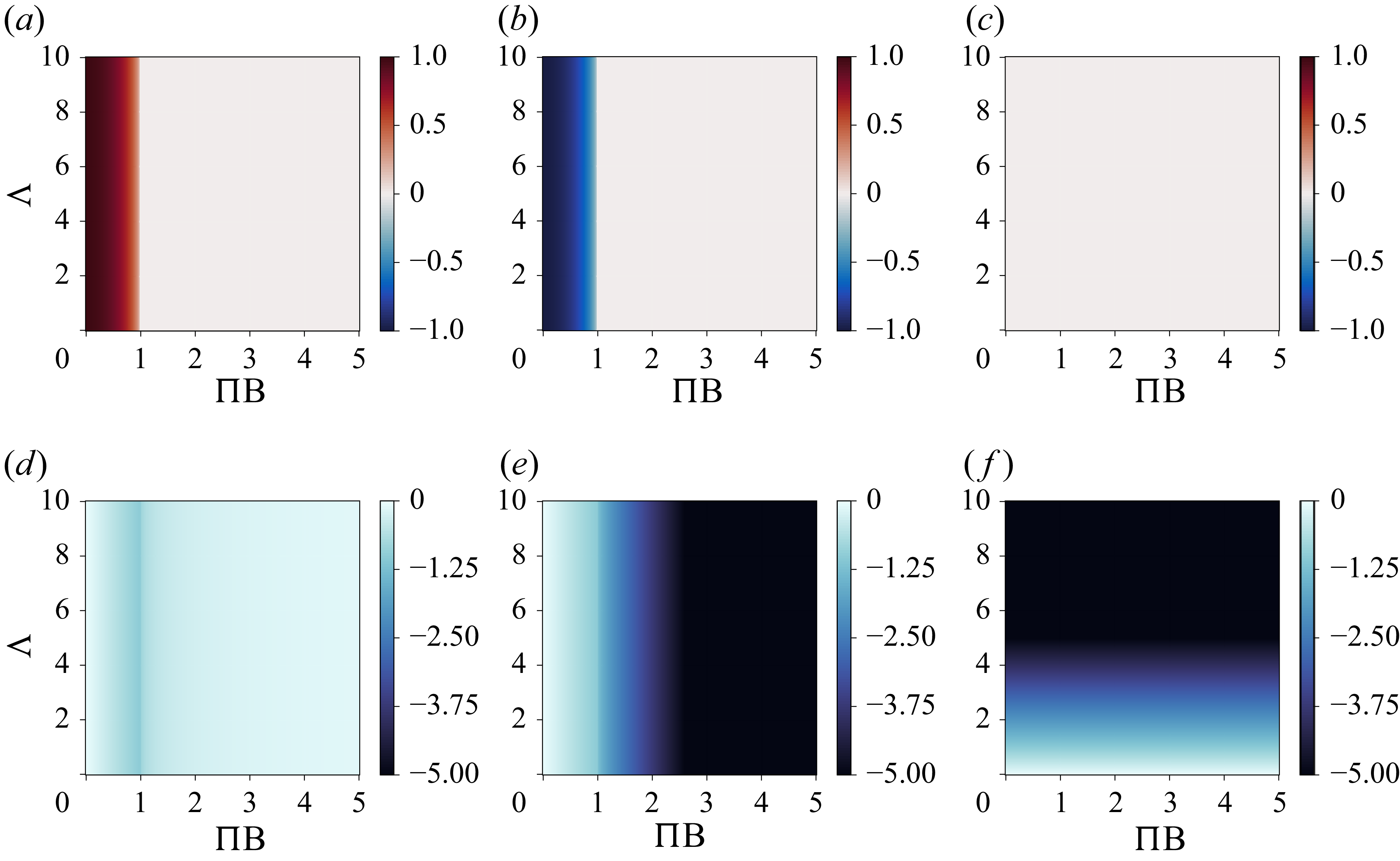


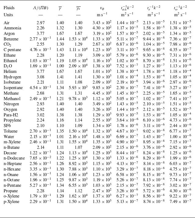


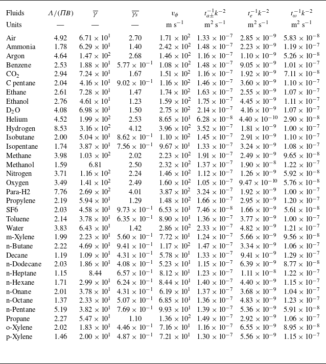


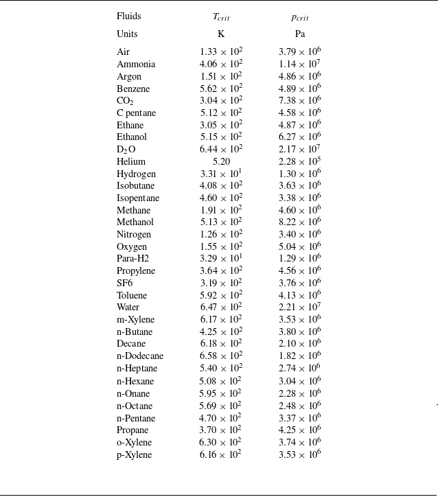

 Open access