


1. Introduction
A compression ramp configuration (i.e. a flat plate followed by a ramp) is representative of many components for high-speed vehicles, such as air inlets, junctions, control surfaces, etc. Fundamental studies of supersonic and hypersonic flows over a compression ramp contribute to an effective design of high-speed vehicles. On the other hand, for hypersonic flight, the vehicle requires blunted leading edges to reduce the high stagnation-point heating loads. Hence, it is of practical importance to investigate hypersonic compression-ramp flows with leading-edge bluntness. Essentially, a hypersonic compression-ramp flow is dominated by shock-wave/boundary-layer interaction (SWBLI). However, the presence of a blunt leading edge complicates the flow phenomenon. Firstly, owing to the formation of a strong bow shock ahead of the leading edge, the flow conditions encountered by the compression ramp, such as Mach number and Reynolds number, are modified with respect to the sharp leading-edge case. As a result, aerodynamic effects such as friction drag and surface heating are inevitably altered. Secondly, an entropy layer is generated behind the curved leading-edge shock. This entropy layer interacts with the downstream boundary layer over the compression ramp and therefore affects flow separation.
Studies concerning leading-edge bluntness effects mainly focus on the two-dimensional (2-D) flow structure. In terms of SWBLI on a compression ramp, a strong adverse pressure gradient induced by the ramp shock can lead to boundary-layer separation upstream of the corner. By conducting extensive experimental studies, Holden (Reference Holden1971) and Gray & Rhudy (Reference Gray and Rhudy1973) found that the size of the separated region was increased by applying a small blunting to the leading edge, whereas the length of the separated region dropped as the leading-edge bluntness was further increased. This phenomenon is referred to as the reversal trend of flow separation. Holden (Reference Holden1971) related the reversal trend to the bluntness–viscous interaction theoretically described by Cheng et al. (Reference Cheng, Hall, Golian and Hertzberg1961). According to their studies, the boundary-layer displacement effects are dominant prior to the reversal point, while the leading-edge bluntness effects dominate the region where the size of the separated flow drops. In addition to experimental studies, recent numerical investigations highlighted that the relative thickness of the boundary layer and entropy layer upstream of separation is responsible for the variation in separation-bubble size (John & Kulkarni Reference John and Kulkarni2014). It is further noted that the reversal trend of flow separation is not restricted to compression-ramp flows, but also occurs for other cases of SWBLI, such as shock impingement on a flat plate (Sriram et al. Reference Sriram, Srinath, Devaraj and Jagadeesh2016), a double cone (Hao & Wen Reference Hao and Wen2020) and a double wedge (Neuenhahn & Olivier Reference Neuenhahn and Olivier2006).
In contrast to the well documented 2-D phenomena, studies concerning the occurrence of three-dimensionality in hypersonic compression-ramp flows are relatively sparse. Although three-dimensionality has been observed for compression-ramp flows, the physical mechanism underlying the observed phenomena is only partially understood. The most remarkable phenomenon is the streamwise heat-flux streaks formed on the ramp surface, which has been reported in numerous experimental (Ginoux Reference Ginoux1971; Simeonides & Haase Reference Simeonides and Haase1995; Roghelia et al. Reference Roghelia, Olivier, Egorov and Chuvakhov2017b; Chuvakhov & Radchenko Reference Chuvakhov and Radchenko2020) and numerical (Ohmichi & Suzuki Reference Ohmichi and Suzuki2013; Cao, Klioutchnikov & Olivier Reference Cao, Klioutchnikov and Olivier2019; Dwivedi et al. Reference Dwivedi, Sidharth, Nichols, Candler and Jovanović2019) studies. Conventionally, the streamwise streaks are attributed to the formation of Görtler vortices supported by the concave flow curvature in the reattaching flow regions (Ginoux Reference Ginoux1971; Simeonides & Haase Reference Simeonides and Haase1995). However, recent numerical studies demonstrated the formation of heat-flux streaks on the ramp even without introducing any artificial disturbances (Ohmichi & Suzuki Reference Ohmichi and Suzuki2013; Klioutchnikov, Cao & Olivier Reference Klioutchnikov, Cao and Olivier2017). Moreover, Cao et al. (Reference Cao, Hao, Klioutchnikov, Olivier and Wen2021) identified a low-frequency unsteadiness for the heat-flux streaks in a compression-ramp flow without upstream disturbances. These facts indicate the presence of a mechanism intrinsic to the flow system.
It is known that a 2-D separated flow has the potential to support self-excited global instability (Theofilis Reference Theofilis2011). Global stability analysis (GSA) is used to study the linear stability of small-amplitude perturbations superposed on a steady base flow without assumptions on the spatial variation of the base flow and the directionality of perturbation waves. This makes GSA suitable for studying the stability of flows with separation (Sidharth et al. Reference Sidharth, Dwivedi, Candler and Nichols2018). By performing GSA for a double-wedge flow, Sidharth et al. (Reference Sidharth, Dwivedi, Candler and Nichols2018) identified the onset of three-dimensionality in the separated region, which was induced by intrinsic instabilities and resulted in temperature streaks on an adiabatic wall. The revealed global unstable mode was shown to originate from the streamwise deceleration of the recirculating flow, rather than centrifugal effects. More recently, Cao et al. (Reference Cao, Hao, Klioutchnikov, Olivier and Wen2021) studied a hypersonic compression-ramp flow with a sharp leading edge (Roghelia et al. Reference Roghelia, Olivier, Egorov and Chuvakhov2017b) using direct numerical simulation (DNS) and GSA. The temporal growth rate, the length scale of heat-flux streaks and the spatial structure of the global modes (both stationary and oscillatory) identified by the DNS were well predicted by the GSA. The aforementioned work provides evidence for the significance of intrinsic instability to the occurrence of three-dimensionality.
The present study considers the hypersonic compression-ramp flows experimentally investigated by Roghelia et al. (Reference Roghelia, Chuvakhov, Olivier and Egorov2017a,Reference Roghelia, Olivier, Egorov and Chuvakhovb), where streamwise heat-flux streaks were observed on the ramp surface for small leading-edge radii. Interestingly, as mentioned by Roghelia et al. (Reference Roghelia, Chuvakhov, Olivier and Egorov2017a), heat-flux streaks disappeared when the leading-edge radius was sufficiently large. Based on the aforementioned information, it is conjectured that the presence and absence of the heat-flux streaks are connected to the intrinsic instability which varies with the leading-edge radius. To verify this hypothesis, we employ GSA and DNS to investigate the hypersonic compression-ramp flows in Roghelia et al. (Reference Roghelia, Chuvakhov, Olivier and Egorov2017a). A wide range of leading-edge radii is considered to examine its influence on flow separation and global instability, as well as surface heat transfer.
The reminder of the paper is organised as follows. Numerical methodology including DNS and GSA is described in § 2. The reversal trend of the flow separation as a result of varying leading-edge radius is discussed in § 3. In § 4, GSA and DNS are performed to examine the effects of leading-edge bluntness on the global instability of the compression-ramp flows. Leading-edge bluntness effects on surface heat transfer are provided in § 5. Conclusions are given in § 6.
2. Numerical methodology
2.1. DNS
Direct numerical simulations achieved by a finite-difference method of high-order accuracy in space and time and with shock capturing ability is applied to study the hypersonic compression-ramp flow problem. The three-dimensional (3-D) Navier–Stokes equations for unsteady, compressible flow are employed in a conservative form, and can be written as
 \begin{equation} \frac{\partial U}{\partial t} + \frac{\partial F}{\partial x} + \frac{\partial G}{\partial y} + \frac{\partial H}{\partial z} = \frac{\partial F_\nu}{\partial x} + \frac{\partial G_\nu}{\partial y} + \frac{\partial H_\nu}{\partial z}, \end{equation}
where  $U = (\rho , \rho u, \rho v, \rho w, \rho e)^\textrm {T}$ is the vector of conservative variables, $\rho$ is the density, $u, v$ and $w$ are the flow velocities and $e$ is the total energy per unit mass. The equation system is closed by the perfect gas law relating pressure, density and temperature, as well as Sutherland's law for calculating the viscosity.
In terms of the numerical methods, time integration is performed by an explicit third-order total variation diminishing Runge–Kutta scheme. A weighted, essentially non-oscillatory, fifth-order finite-difference scheme is applied for the discretisation of the inviscid fluxes, based on the work of Jiang & Shu (Reference Jiang and Shu1996). A sixth-order central-difference scheme is used to approximate the viscous fluxes. The DNS solver has been validated and successfully applied to study hypersonic compression-ramp flows (Cao et al. Reference Cao, Klioutchnikov and Olivier2019; Cao, Klioutchnikov & Olivier Reference Cao, Klioutchnikov and Olivier2020; Cao et al. Reference Cao, Hao, Klioutchnikov, Olivier and Wen2021).
As for the boundary conditions, free-stream parameters are prescribed at the upper boundary (blunt leading-edge cases). A zero-gradient extrapolation condition is used for the out-flow boundary. For the no-slip wall, isothermal conditions are specified with the wall temperature being 293 K. Periodic boundary conditions are applied in the spanwise direction.
2.2. GSA
The governing equations (2.1) are linearised by decomposing  $U$ into a 2-D base flow $U_\text {2-D}$ and a 3-D small-amplitude perturbation $U'$ as
 \begin{equation} U(x,y,z,t) = U_\text{2-D}(x,y) + U'(x,y,z,t). \end{equation}
It is also assumed that  $U_\text {2-D}$ satisfies the 2-D Navier–Stokes equations. The linearised governing equations are then discretised using a second-order finite-volume method. The inviscid fluxes are evaluated using the modified Steger–Warming scheme (MacCormack Reference MacCormack2014) near discontinuities to eliminate numerical noise and a simple arithmetic average in smooth regions to reduce numerical dissipation, respectively. The viscous fluxes are calculated using a second-order central-difference scheme. Details of the inviscid and viscous fluxes were provided by Sidharth et al. (Reference Sidharth, Dwivedi, Candler and Nichols2018).
In this study, we consider the temporal stability of a spanwise periodic perturbation in the following harmonic-wave form:
 \begin{equation} U'(x,y,z,t) = \hat{U}(x,y) \exp[-\textrm{i}(\omega_r + \textrm{i}\omega_i) t + \textrm{i} \beta z] + \text{complex conjugate}, \end{equation}
where  $\hat {U}$ is the eigenfunction, $\omega _r$ is the angular frequency, $\omega _i$ is the growth rate and $\beta$ is the spanwise wavenumber. The corresponding frequency and spanwise wavelength are defined by $f = \omega _r / 2 {\rm \pi}$ and $\lambda _z = 2 {\rm \pi}/ \beta$, respectively.
Substituting (2.3) into the linearised Navier–Stokes equations results in an eigenvalue problem, which is solved using the implicit restarted Arnoldi method implemented in ARPACK (Sorensen et al. Reference Sorensen, Lehoucq, Yang and Maschhoff1996). A shift-invert approach is adopted to efficiently explore the eigenvalue spectrum for a given  $\beta$.
3. Reversal trend of flow separation
3.1. Flow conditions and geometry
The numerically considered flow conditions and compression-ramp geometry are based on those used in the experimental campaign carried out in the hypersonic Aachen Shock Tunnel TH2 at the Shock Wave Laboratory of RWTH Aachen University (Roghelia et al. Reference Roghelia, Chuvakhov, Olivier and Egorov2017a,Reference Roghelia, Olivier, Egorov and Chuvakhovb). A comprehensive study, involving experiments (Roghelia et al. Reference Roghelia, Olivier, Egorov and Chuvakhov2017b) and numerical simulations (Cao et al. Reference Cao, Hao, Klioutchnikov, Olivier and Wen2021) has provided a detailed description for the case of a sharp leading edge. Hence, the same flow conditions as for the sharp leading-edge case are used for the blunt leading-edge cases. The free-stream Mach number ( $M_\infty$) and unit Reynolds number ( $Re_\infty$) are 7.7 and $4.2 \times 10^6\ \text {m}^{-1}$, respectively. The inflow (air) is assumed to be a calorically perfect gas owing to a relatively low total enthalpy ( $h_0 = 1.7$ MJ kg $^{-1}$), that is, the specific heat ratio equals 1.4. The constant wall temperature ( $T_w$) is given by 293 K, which corresponds to a wall-to-total temperature ratio of 0.18.
For the compression-ramp geometry, a flat plate of length ( $L$) 100 mm is followed by a ramp with a deflection angle of 15 $^{\circ }$. The length of the ramp for the blunt leading-edge cases equals 120 mm. The leading-edge radius ranges from 0.15 to 2.5 mm. In particular, 11 cases are considered in the present study, for which the radii are 0.15, 0.3, 0.5, 0.7, 1, 1.3, 1.4, 1.5, 1.7, 2 and 2.5 mm. For convenience, these cases, together with the sharp leading-edge case, are labelled as R0, R015, R03, R05, R07, R1, R13, R14, R15, R17, R2 and R25, respectively.
In terms of mesh distribution, the number of grid points in streamwise ( $x$) and wall-normal ( $y$) directions is 1600 and 300, respectively. The mesh is clustered at the leading edge and near the wall, yielding a non-dimensional wall distance of $\varDelta y_{wall} / L \approx 9 \times 10^{-5}$ at the separation position for all cases. Note that the boundary-layer flow upstream of separation is laminar. Based on the set-up described above, the time step is set as $3 \times 10^{-9}$ s to ensure that the Courant–Friedrichs–Lewy number remains less than one. It is important to note that the mesh resolution in the $x$–
$x$– $y$ plane for the blunt leading-edge cases is higher than that for the sharp leading-edge case ( $1080\times 240$), which has been shown to be sufficient to capture the flow separation (Cao et al. Reference Cao, Hao, Klioutchnikov, Olivier and Wen2021). Nevertheless, preliminary simulations have been performed to verify the grid independence of our present results.
3.2. Reversal trend of the separation-bubble length
The reversal trend of flow separation caused by the leading-edge bluntness is shown in the following on the basis of the DNS results. Figure 1 presents the Mach number contour for cases R0, R015, R05, R1, R15 and R2. As can be observed, the size of the separation bubble (the blue region) increases when the leading-edge radius is increased from 0 to 0.15 mm. A further growth of the separation bubble is found when the radius is increased to 0.5 mm. However, as the radius rises from 1 to 2 mm, the size of the separation bubble decreases monotonically.

Figure 1. Mach number contour for cases with different leading-edge radii. (a) R = 0; (b) R = 0.15 mm (c) R = 0.5 mm; (d) R = 1 mm; (e) R = 1.5 mm; ( f) R = 2 mm.
To better illustrate the reversal trend of flow separation, the variation of separation and reattachment positions together with the variation of separation-bubble length ( $L_b$), which is defined as the streamwise distance between the separation and reattachment positions, with the leading-edge radius are presented in figure 2. It is seen from figure 2(a) that the separation point reaches its most upstream position when $R = 0.3$ mm. However, the farthest downstream position for the reattachment point occurs for case R07. The combined variation of separation and reattachment positions results in a reversal trend for the separation-bubble length, as shown in figure 2(b). The critical radius for the reversal trend is $R = 0.5$ mm. This reversal trend and the observed critical radius are consistent with experimental measurements (Roghelia et al. Reference Roghelia, Chuvakhov, Olivier and Egorov2017a). In the following, a comprehensive study aiming to reveal the occurrence of three-dimensionality in the compression-ramp flows is conducted.

Figure 2. Variation of (a) the separation (square) and reattachment (diamond) positions and (b) the separation-bubble length with leading-edge radius.
4. Effect of leading-edge bluntness on global instability
4.1. Global stability analysis with respect to the 2-D base flows
In this section, GSA is performed to reveal the effect of leading-edge bluntness on the intrinsic instability of the compression-ramp flow. The 2-D solutions for different nose radii obtained in § 3 are used as the base flows of GSA. To reduce the computational cost, especially memory usage, the numerical solutions are interpolated on a coarse grid ( $600\times 200$). Grid independence was verified by using a finer grid ( $800 \times 300$). To facilitate a clear comparison, the GSA results for case R0 obtained in our previous study (Cao et al. Reference Cao, Hao, Klioutchnikov, Olivier and Wen2021) are also presented.
Figure 3 shows the growth rates of the most unstable modes as a function of  $\lambda _z$ for cases R0, R05, R1 and R2. In each subfigure, the vertical line indicates the spanwise wavelength where the largest growth rate occurs. The eigenvalue spectra at these wavelengths are plotted in figure 4. For case R0, three branches of unstable modes were identified. Here, the leading stationary and oscillatory unstable modes are denoted by modes 1 and 2, with their growth rates peaking at $\lambda _z / L = 0.066$ and 0.070, respectively. The third branch is also an oscillatory mode, which is insignificant because of its low growth rate. When the leading-edge bluntness is increased to 0.5 mm, i.e. the critical radius, the flow system is substantially destabilised, a feature highlighted by the coexistence of multiple unstable modes (see figure 4b). The largest growth rate is increased by a factor of 2 with the corresponding wavelength shifted to $\lambda _z / L = 0.105$. In addition, two further stationary unstable modes can be observed. For case R1, the flow system is stabilised compared with case R05. The wavelength corresponding to the largest growth rate is reduced to $\lambda _z / L =$ 0.084. For case R2, only one stationary unstable mode can be identified. Its low growth rate indicates that the flow system is marginally unstable. Although not shown here, further increasing the nose radius monotonically stabilises the compression-ramp flow until the system becomes globally stable. It is also interesting to note that the non-dimensional frequency of the leading oscillatory mode (mode 2) is largely unchanged, which is approximately 0.2 for different nose radii.

Figure 3. Growth rates of the most unstable modes as a function of spanwise wavelength for cases (a) R0; (b) R05; (c) R1 and (d) R2. The vertical dash-dotted lines correspond to  $\lambda _z / L = 0.066, 0.105, 0.084$ and 0.180, respectively.

Figure 4. Eigenvalue spectra for cases (a) R0 at  $\lambda _z / L = 0.066$; (b) R05 at $\lambda _z / L = 0.105$; (c) R1 at $\lambda _z / L = 0.084$; (d) R2 at $\lambda _z / L = 0.180$.
By comparing the growth rates of the most unstable modes (mode 1) for cases R0, R05, R1 and R2, which are  $\omega _i L / U_\infty = 0.51$, 1.04, 0.82 and 0.05, respectively, it is clear that the growth rate exhibits a reversal trend. In other words, the amplification rate of 3-D perturbations initially increases and then decreases with increasing leading-edge radius. In summary, the GSA results demonstrate a reversal trend for the intrinsic instability of the considered compression-ramp flows.
4.2. Verification by DNS
In the following, DNS is performed to verify the intrinsic instability revealed by the GSA. For the 3-D simulations, the width of the physical domain equals 50 mm for the blunt leading-edge cases (R05, R1 and R2). Note that the spanwise width of the physical domain for the sharp leading-edge case was 100 mm (Cao et al. Reference Cao, Hao, Klioutchnikov, Olivier and Wen2021), whereas in experiments models of 200 mm width were used for both sharp and blunt leading-edge cases (Roghelia et al. Reference Roghelia, Chuvakhov, Olivier and Egorov2017a). As shown by Cao et al. (Reference Cao, Hao, Klioutchnikov, Olivier and Wen2021), when the spanwise width was reduced from 100 to 30 mm, both saturated flows exhibit similar surface heat-flux streaks and almost identical wall parameters (pressure, Stanton number). This is expected because a periodic boundary condition is used in the spanwise direction. Therefore, a width of 50 mm is chosen for the blunt leading-edge cases in order to reduce the computational costs. In the spanwise direction ( $z$), 300 grid points are placed with a constant spacing $\varDelta z / L = 1.67 \times 10^{-3}$. This resolution is slightly higher than that for the sharp leading-edge case ( $\varDelta z / L = 2.08 \times 10^{-3}$).
The initial 3-D flow fields are generated by duplicating the 2-D solutions discussed in § 3, in the spanwise direction. For case R0, initial values for the spanwise velocity (randomised between  $-0.01 \leq w/U_\infty \leq 0.01$) are introduced on the first twenty grid points normal to the wall between $0.5 < x/L < 1.5$ (Cao et al. Reference Cao, Hao, Klioutchnikov, Olivier and Wen2021), while the initial spanwise velocity is set to zero for the blunt leading-edge cases. It is demonstrated in Appendix that the introduction of initial randomised spanwise velocity has no remarkable influence on the occurrence of the unstable modes, and that the growth of instability waves can arise from the extremely low-level perturbations provided by numerical round-off error. No external disturbances are introduced at the inflow or at the wall, which enables the examination of intrinsic instabilities in the fluid-dynamic system.
To capture the growth of three-dimensionality, we consider the temporal evolution of the absolute value of spanwise velocity at a streamwise position, which is defined as
 \begin{equation} \bar{w} = \sqrt{\frac{1}{N_y N_z} \sum_{j=1}^{N_y} \sum_{k=1}^{N_z} (w/U_\infty)_{j,k}^2}, \end{equation}
where  $N_y$ and $N_z$ denote the number of grid points in wall-normal and spanwise directions, respectively. Figure 5 shows the temporal history of $\bar {w}$ at $x/L = 1.04$ for case R0, at $x/L = 1.13$ for case R05, at $x/L = 1.16$ for case R1 and at $x/L = 1.05$ for case R2. These streamwise positions were chosen because $\bar {w}$ is largest here for all streamwise positions. It should be mentioned that these positions are located in the separated region as the instability core lies inside the separation bubble (Sidharth et al. Reference Sidharth, Dwivedi, Candler and Nichols2018; Cao et al. Reference Cao, Hao, Klioutchnikov, Olivier and Wen2021). The slope of the dotted lines shown in figure 5 corresponds to the growth rate of the most unstable mode identified by GSA (i.e. mode 1 in figure 4a–c).

For cases R0, R05 and R1, after an initial adaption,  $\bar {w}$ experiences an exponential growth, and the growth rates are close to those predicted by GSA. Subsequent to the linear growth stage, a nonlinear saturation takes place until the quasi-steady state is achieved. It should be mentioned that the relatively long adaption period for case R05 may be attributed to the large separation-bubble size and the multiple recirculating vortices inside the primary bubble induced by the secondary separation near the corner (Gai & Khraibut Reference Gai and Khraibut2019).
The previous GSA revealed that the growth rate of the global mode for case R2 is close to zero. As seen in figure 5, the magnitude of  $\bar {w}$ remains at a very low level corresponding to the numerical noise. In other words, the flow field for case R2 remains stable during the simulated time period. Although the simulation is run up to $tU_\infty /L = 32$, and a further simulation is not considered owing to the limitation of computing resources, the stabilising effect for large leading-edge radii is in line with experimental results. As mentioned by Roghelia et al. (Reference Roghelia, Chuvakhov, Olivier and Egorov2017a), surface heat-flux streaks were not visible for large leading-edge radii.
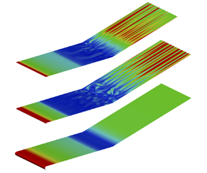
Figure 6 shows instantaneous spanwise velocity fields ( $w/U_\infty$) in the $x$–
$x$– $y$ and $z$–
$z$– $y$ planes for cases R0, R05 and R1. The corresponding time instants are $tU_\infty /L = 9$, 17 and 10, respectively, which are located at the exponential growth stage (see figure 5). Note that for case R0 (figure 6b), only half the spanwise length is shown in order to be consistent with figure 6(d,f). It is apparent that the onset of three-dimensionality lies inside the separation bubble, and that the flow fields are characterised by a spanwise periodicity, with the dominant spanwise wavelengths being $\lambda _z / L \approx 0.067$, 0.1 and 0.083, respectively. These wavelengths coincide with those of the most unstable modes identified by GSA (see figure 3). It should be mentioned that the instability waves do not exhibit a strict uniformity, i.e. the wavelength of each wave is not identical, especially for case R05. The reasons are twofold. Firstly, the spanwise width of the physical domain does not fit in with the whole-number multiples of the wavelength of the most unstable global mode revealed by the GSA (i.e. $L_z/\lambda _z$ is not an integer). As shown in Appendix, letting $L_z/\lambda _z = 4$, a better match in the wavelength is achieved between GSA and DNS. However, a similar non-uniformity is still present for cases A1 and A2 (see Appendix). Secondly, and more importantly, as uncovered by the GSA, for cases R0, R05 and R1, there exist several unstable modes whose growth rates peak at different wavelengths. Although the mode with the largest growth rate dominates the growth of perturbations, other modes can also be present and affect the spanwise periodicity. As shown in Cao et al. (Reference Cao, Hao, Klioutchnikov, Olivier and Wen2021) (case R0), the footprint of mode 2 could be identified in the exponential growth stage. In the present simulations, a fixed but relatively large spanwise width is used allowing the competition or interaction of different unstable modes, which also facilitates the later discussion for the saturated flows.

Figure 6. Instantaneous distribution of spanwise velocity for case R0 at  $tU_\infty /L = 9$ in (a) $x$–
$x$– $y$ plane at $z/L = 0.24$ and (b) $z$–
$z$– $y$ plane at $x/L = 1.04$; for case R05 at $tU_\infty /L = 17$ in (c) $x$–
$x$– $y$ plane at $z/L = 0.35$ and (d) $z$–
$z$– $y$ plane at $x/L = 1.13$; for case R1 at $tU_\infty /L = 10$ in (e) $x$–
$x$– $y$ plane at $z/L = 0.13$ and (f) $z$–
$z$– $y$ plane at $x/L = 1.16$. The solid circles highlight the separation and reattachment positions. Flow fields are obtained from DNS data.
In general, the matching growth rates and spanwise wavelengths between GSA and DNS results provide firm support for the fact that the occurrence of three-dimensionality in the compression-ramp flows is triggered by the instabilities intrinsic to the flow system. In the following, we focus on the leading-edge bluntness effects on the surface heat transfer with respect to the saturated flow.
5. Leading-edge bluntness effects on surface heat transfer
Instantaneous distributions of wall Stanton number for cases R0, R05, R1 and R2 are presented in Figure 7, the dimensionless number is defined as
 \begin{equation} St = \frac{q_w}{\rho_\infty U_\infty c_p (T_{aw} - T_w)}. \end{equation}
Here,  $q_w$ denotes the surface heat flux, $c_p$ is the specific heat capacity and $T_{aw}$ is the adiabatic wall temperature. We emphasise that the chosen flow fields are in the quasi-steady state (see figure 5), where the flow has fully saturated and deviates from that at the exponential growth stage. Separation and reattachment positions are highlighted by iso-lines of zero skin-friction coefficient ( $C_f$). The meandering reattachment line is indicative of a 3-D reattaching process. As a consequence of the flow unsteadiness originating from the intrinsic instability (Cao et al. Reference Cao, Hao, Klioutchnikov, Olivier and Wen2021), a non-uniform spanwise distribution of heat-flux streaks is present on the ramp surface for cases R0, R05 and R1. As expected, there exists no spanwise variation for the wall Stanton number for case R2 as the flow remains 2-D at this time instant.

Figure 7. Instantaneous distribution of wall Stanton number for cases (a) R0 at  $tU_\infty /L = 60$, (b) R05 at $tU_\infty /L = 32$, (c) R1 at $tU_\infty /L = 32$ and (d) R2 at $tU_\infty /L = 32$. Black solid lines denote iso-lines of $C_f = 0$. Flow from left to right.
To summarise the effects of leading-edge bluntness on the aerodynamic heating on the ramp surface, figure 8(a) shows the streamwise distribution of the spanwise-averaged wall Stanton number obtained from figure 7. The dashed lines represent the values obtained from the 2-D base flows. Interestingly, the heating loads downstream of reattachment exhibit a monotonic decrease as the leading-edge radius is increased, although a reversal trend is present for the separation-bubble length and the intrinsic instability. The decrease in the peak heating value is consistent with experimental results (Roghelia et al. Reference Roghelia, Chuvakhov, Olivier and Egorov2017a). Compared with the 2-D solutions, an increase in the Stanton number is present downstream of reattachment for the 3-D results. Specifically, the peak Stanton number increases by 3 %, 35 % and 36 % for cases R0, R05 and R1, respectively. It should be noted that the 3-D values are spanwise-averaged. In figure 8(b), the peak heating value along with its spanwise variation obtained from figure 7 are plotted against the leading-edge radius. The root-mean-square value for the spanwise variation is approximately  $7.5 \times 10^{-4}$ for cases R0, R05 and R1. In short, the presence of three-dimensionality in the flow field causes an elevated heating level downstream of reattachment in comparison with 2-D solutions.

Figure 8. (a) The solid lines represent the streamwise distribution of spanwise-averaged wall Stanton number corresponding to figure 7. The dashed lines correspond to the 2-D base flow. (b) Variation of heating peak near reattachment with leading-edge radius. The vertical bar provides the root-mean-square value of the spanwise variation of wall Stanton number at the peak heating position.
6. Conclusions
In this work, hypersonic compression-ramp flows with different leading-edge radii were considered with a free-stream Mach number of 7.7 and a unit Reynolds number of  $4.2 \times 10^6$ m $^{-1}$. The DNS and GSA were performed to study the effects of leading-edge bluntness on flow separation, the intrinsic instability and surface heat transfer. Similar to the well known reversal trend of flow separation, a reversal trend was revealed for the intrinsic instability. When the leading-edge radius is increased from zero to the critical value (0.5 mm), the compression-ramp flow becomes more unstable, with the unstable modes being characterised by higher growth rates. Then, when the leading-edge radius is further increased, the flow tends to be more stable.
As a result of the three-dimensionality triggered by the intrinsic instability, streamwise heat-flux streaks are formed on the ramp surface downstream of reattachment. Unlike the reversal trend of the flow separation and intrinsic instability, the peak heating value exhibits a monotonic decrease as the leading-edge radius is increased. More importantly, because the flow becomes globally stable when the leading-edge radius is sufficiently large, the spanwise variation of surface heat flux disappears, which accounts for the experimental observations (Roghelia et al. Reference Roghelia, Chuvakhov, Olivier and Egorov2017a). Therefore, the present study demonstrates that a proper blunting of the leading edge can suppress flow separation, reduce aerodynamic heating and stabilise the flow system for a hypersonic compression-ramp flow.
It is interesting to note that the present work shows the formation of heat-flux streaks in the absence of external disturbances. This scenario highlights the importance of the intrinsic instability in the compression-ramp flow system, as addressed by Sidharth et al. (Reference Sidharth, Dwivedi, Candler and Nichols2018) and Cao et al. (Reference Cao, Hao, Klioutchnikov, Olivier and Wen2021). On the other hand, convective mechanisms such as baroclinic effects can play a role in the amplification of extrinsic disturbances, resulting in the formation of heat-flux streaks in an intrinsically stable compression-ramp flow, as demonstrated by Dwivedi et al. (Reference Dwivedi, Sidharth, Nichols, Candler and Jovanović2019). Furthermore, the role of convective mechanisms in an inherently unstable compression-ramp flow is still not fully understood. In experiments involving supersonic and hypersonic flows, it is hard to exclude external disturbances (e.g. free-stream disturbances, surface roughness). Therefore, the observed 3-D phenomena may be triggered by either intrinsic or convective mechanisms or both, which may hinder thorough and rigorous explanations for these phenomena. Because much experimental work has already provided a wealth data, further theoretical and numerical work is required to study these case-dependent scenarios.
Funding
This work was jointly supported by RWTH Aachen University and The Hong Kong Polytechnic University. The authors gratefully acknowledge the computing time granted by the JARA Vergabegremium and provided on the JARA Partition part of the supercomputer CLAIX at RWTH Aachen University under project JARA0218.
Declaration of interests
The authors report no conflict of interest.
Appendix. Influence of the initial spanwise velocity and the spanwise width on numerical solutions
To clarify the influence of initial spanwise velocity and spanwise width on the numerical results, we performed two additional simulations (cases A1 and A2) for the sharp leading-edge case, which are listed in table 1. The spanwise width equals  $L_z/L = 0.2667$, which is equal to four times the wavelength of the most unstable mode (mode 1 in figure 3a), i.e. $L_z/\lambda _z = 4$. Similar to case R0, randomised initial values for the spanwise velocity (ranging at $-0.01 \leq w/U_\infty \leq 0.01$) are introduced on the first twenty grid points normal to the wall between $0.5 < x/L < 1.5$ for case A1. For case A2, the initial spanwise velocity is zero, and the numerical round-off error provides a low-level perturbation for the growth of instability modes.
Table 1. Cases for clarifying the influence of initial spanwise velocity and spanwise width on the numerical solutions.

Figure 9 presents the temporal evolution of  $\bar {w}$ at $x/L = 1.04$ for cases A1 and A2, in comparison with case R0. As an initial spanwise velocity is introduced for case A1, the value of $\bar {w}$ for case A1 is of the order of $10^{-4}$ at $tU_\infty /L = 0$. The subsequent growth of $\bar {w}$ is quite similar to that for case R0, and the growth rate is in line with the GSA prediction. For case A2, however, the value of $\bar {w}$ at the very beginning is of the order of $10^{-6}$. After a relatively long adaption period ( $0 < tU_\infty /L < 7$), the exponential growth of unstable modes commences. The growth rate also agrees with the GSA result. It is worth mentioning that the introduction of an initial value for the spanwise velocity leads to an earlier start of the exponential growth, thus a shorter computational time and fewer computing resources. Furthermore, the comparison between cases R0 and A1 also demonstrates that the spanwise width of the physical domain has no influence on the growth rate.

Figure 9. Temporal evolution of the absolute spanwise velocity (4.1) at  $x/L = 1.04$ for cases R0, A1 and A2. The slope of the dotted lines represents the growth rates of the most unstable modes predicted by GSA.
The occurrence of instability waves for cases A1 and A2 is addressed in the following. Figure 10 compares the spanwise velocity fields extracted from the exponential growth stage. The distribution of spanwise velocity in the  $x$–
$x$– $y$ plane is nearly identical for cases A1 and A2, and it also matches the distribution of spanwise velocity for case R0 (see figure 6a). Obviously, there exist four waves in the spanwise direction, although their wavelengths are not absolutely the same. Therefore, allowing the spanwise width to be the whole-number multiple of the wavelength of the unstable modes can lead to a better agreement between the GSA and DNS results regarding the spanwise wavelength. However, the non-uniformity of instability waves in the spanwise direction is still present and may be supposed to be mainly influenced by the co-existence of several unstable modes. The situation is more severe for case R05 (see figure 6d) because a large number of unstable modes are found by the GSA. One may expect that a uniform distribution of instability waves is present for a case with only one unstable mode, e.g. as shown in Sidharth et al. (Reference Sidharth, Dwivedi, Candler and Nichols2018).

Figure 10. Instantaneous distribution of spanwise velocity for case A1 at  $tU_\infty /L = 9$ in (a) $x$–
$x$– $y$ plane at $z/L = 0.13$ and (b) $z$–
$z$– $y$ plane at $x/L = 1.04$; for case A2 at $tU_\infty /L = 15$ in (c) $x$–
$x$– $y$ plane at $z/L = 0.10$ and (d) $z$–
$z$– $y$ plane at $x/L = 1.04$. The solid circles highlight the separation and reattachment positions.
In summary, the previous discussion shows that the introduction of an initial spanwise velocity field with the chosen spanwise width of the physical domain has no remarkable influence on the occurrence and growth of instability modes in the considered compression-ramp flow.


 Open access