


1. Introduction
The exploration, access and measurement of Antarctic subglacial lakes have the potential to address several significant scientific questions regarding Antarctic Ice Sheet history, life in extreme environments, and how subglacial hydrology can influence ice-sheet flow (Siegert, Reference Siegert2016). Important to each of these questions is how water is supplied to, and released from, subglacial lakes. Considerable focus has been given to inputs and outputs associated with water flow across the ice-sheet bed (e.g. Wingham and others, Reference Wingham, Siegert, Shepherd and Muir2006; Fricker and others, Reference Fricker, Scambos, Bindschadler and Padman2007; Wright and others, Reference Wright2012; Fricker and others, Reference Fricker, Siegfried, Carter and Scambos2016) but there has been relatively little investigation constraining basal melt of the overlying ice sheet at the ice/water interface. A characteristic of the ice sheet that can be exploited to constrain both the location and magnitude of basal melting is the englacial structure of the ice sheet, which can be imaged and characterised using radio-echo sounding (RES) (Siegert, Reference Siegert1999; Dowdeswell and Evans, Reference Dowdeswell and Evans2004). Englacial layers, associated with variations in the density, conductivity and crystal fabric of the ice sheet, are assumed to be isochronous and, in most cases, are associated with the burial of palaeo-ice-sheet surfaces (Siegert, Reference Siegert1999). Over subglacial water bodies, and localised areas of high geothermal heat flux, englacial layers can be locally drawn down so that younger layers are found at greater than expected depths in the ice-sheet column, indicative of high rates of subglacial melt (Siegert and others, Reference Siegert, Kwok, Mayer and Hubbard2000; Gudlaugsson and others, Reference Gudlaugsson, Humbert, Kleiner, Kohler and Andreassen2016; Jordan and others, Reference Jordan2018).
Direct melting of the overlying ice sheet into subglacial lakes influences: (i) the pattern and rate of circulation of the water body (Thoma and others, Reference Thoma, Grofeld, Filina and Mayer2009, Reference Thoma2011; Woodward and others, Reference Woodward2010), through determining where water is introduced to the lake; and (ii) subglacial lacustrine sedimentary processes (Bentley and others, Reference Bentley, Siegert, Kennicutt and Bindschadler2011; Smith and others, Reference Smith2018), by influencing where sediments meltout from the overlying ice and are deposited on the lake floor. While basal melting at the ice/water interface does not operate in isolation, i.e. in an open system it will interact with subglacial water flowing between the ice sheet and the bed, improved knowledge of its location and magnitude will enhance the understanding of the drivers of hydrological processes in subglacial lakes.
Numerical modelling of water circulation has been undertaken for three Antarctic subglacial lakes (Pattyn and others, Reference Pattyn, Carter and Thoma2016): Lake Vostok (e.g. Wüest and Carmack, Reference Wüest and Carmack2000; Mayer and others, Reference Mayer, Grosfeld and Siegert2003; Thoma and others, Reference Thoma, Grosfeld and Mayer2008a, Reference Thoma, Mayer and Grosfeldb), Lake Concordia (Thoma and others, Reference Thoma, Grofeld, Filina and Mayer2009) and Subglacial Lake Ellsworth (SLE) (Woodward and others, Reference Woodward2010; Thoma and others, Reference Thoma2011). The most up-to-date water circulation model applied to subglacial lakes, ROMBAX is an adapted 3D ocean model. This model integrates hydrodynamic equations, the geometry of the water body, and a formulation to estimate the mass balance (i.e. rates of melt and refreezing) at the ice/lake interface (Pattyn and others, Reference Pattyn, Carter and Thoma2016). ROMBAX assumes that the lake system is closed (i.e. no lake inflow or outflow). Inclined ice/water interfaces that induce melting in deeper areas and refreezing in higher areas generate water circulation in subglacial lakes. Well-constrained lake geometries are therefore essential for determining the basal mass balance. With constraints on ice flow, the thickness and distribution of accretion ice can be calculated (Woodward and others, Reference Woodward2010). Input data for ROMBAX modelling of Lake Vostok, Lake Concordia and SLE comprise lake bathymetry (i.e. water column thickness) determined from seismic reflection surveys or the inversion of gravity measurements, ice thickness, assumed values of geothermal heatflux and the velocity of ice flow from GPS or InSAR measurements. For each lake, a basal mass balance (i.e. a prediction of where basal melt, causing layer drawdown, and refreezing, causing layer uplift, occurs), the pattern and velocity of water flow, and the extent and thickness of accreted ice, have been determined. In comparison to Lakes Concordia and Vostok, water circulation modelling suggests that SLE has higher rates of basal melt, basal refreezing and more vigorous water circulation (see: Table 1 of Pattyn and others, Reference Pattyn, Carter and Thoma2016). In addition, SLE is positioned at a depth that intersects the Line of Maximum Density (Wüest and Carmack, Reference Wüest and Carmack2000; Thoma and others, Reference Thoma2011); a critical pressure depth (3050 m) between dense water that will sink when warmed (ice overburden pressure <critical water pressure) and water that is buoyant and will rise when warmed (ice overburden pressure >critical water pressure). The physical consequences of this in SLE are that deeper parts of the lake may experience convective (ocean-type) circulation leading to mixing of the water column, while shallower parts may have limited convection and a stratified water column (Woodward and others, Reference Woodward2010; Thoma and others, Reference Thoma2011; Pattyn and others, Reference Pattyn, Carter and Thoma2016). However, the vigorous water circulation induced by the steep ice/water interface at SLE means that water circulation, and hence mixing of the water column, may occur irrespective of the critical pressure boundary (Woodward and others, Reference Woodward2010; Thoma and others, Reference Thoma2011).
The aims of this paper are to report the character and 3D form of the englacial layer package over SLE and its wider catchment, to (i) identify and explain the processes responsible for layer morphology; (ii) assess whether the geometry of the englacial layers is spatially consistent with output from existing numerical models of water circulation in SLE; (iii) improve understanding of the interactions between SLE and the overlying ice sheet (i.e. identifying potential sources of meltwater); (iv) analyse catchment-scale hydrological connectivity; and (v) evaluate conceptual models of sediment deposition in SLE. Our study is justified by the surprisingly few detailed observational investigations (3D or otherwise) of englacial layers over and around subglacial lakes (see: Siegert and others, Reference Siegert, Kwok, Mayer and Hubbard2000; Leonard and others, Reference Leonard, Bell, Studinger and Tremblay2004; Siegert and others, Reference Siegert2004; Tikku and others, Reference Tikku2005; Carter and others, Reference Carter, Blankenship, Young and Holt2009), the unparalleled resolution, detail and tailored survey design of the SLE RES dataset, and the forthcoming exploration of Subglacial Lago CECs (Rivera and others, Reference Rivera, Uribe, Zamora and Oberreuter2015), located not far from SLE, by a UK-Chilean research programme.
2. Subglacial Lake Ellsworth
Between 2007 and 2009 SLE was subject to a comprehensive ground-based geophysical characterisation, including RES, seismic reflection, GPS and shallow ice core measurements, and numerical modelling of water circulation patterns, in advance of an attempt at direct access and exploration in 2012 (Woodward and others, Reference Woodward2010; Ross and others, Reference Ross, Siegert, Kennicutt and Bindschadler2011a; Siegert and others, Reference Siegert2012, Reference Siegert, Makinson, Blake, Mowlem and Ross2014; Smith and others, Reference Smith2018). While the basal topography, water column thickness, nature of the sediments on the lake floor and the catchment-scale subglacial hydrological flow paths have been constrained and published (Ross and others, Reference Ross, Siegert, Kennicutt and Bindschadler2011a; Siegert and others, Reference Siegert2012; Smith and others, Reference Smith2018), few details of the englacial layer form have been reported. Ross and others (Reference Ross2011b) reconstructed Holocene ice flow using englacial layer folding but did not report or discuss the implications of the broader internal layer geometry for SLE. Here, we describe the RES survey of SLE, detailing the geometry and character of englacial layers in the SLE RES dataset. This is the first time that this dataset has been reported and described. We also present a high-resolution DEM of the outlet area of SLE.
3. Methods
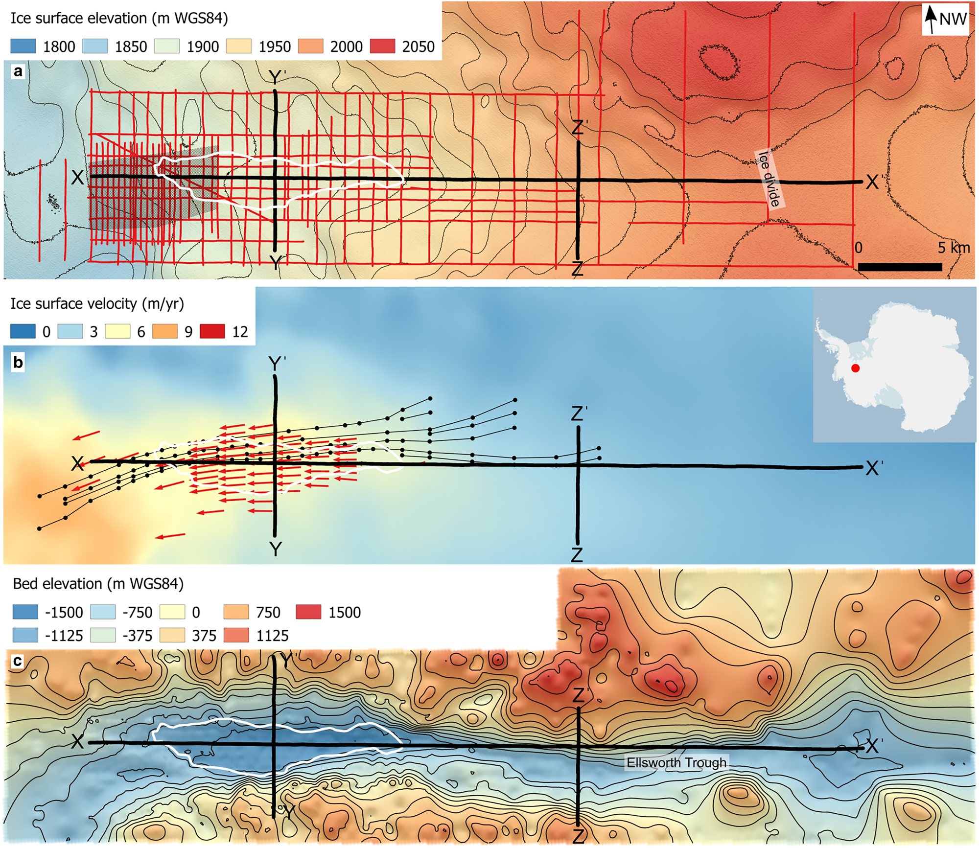
The RES survey used the ground-based ~1.7 MHz pulsed DEep-LOok-Radar-Echo-Sounder (DELORES) RES system (King and others, Reference King, Pritchard and Smith2016) towed by a snow mobile at an average rate of ~12 km hr−1. Traces, comprising the stacking of 1000 measurements, were acquired at an approximate along-track sampling resolution of 3–4 m. The survey (Fig. 1a) was designed to characterise the physical system of the subglacial environment, from the ice divide to beyond the down-ice end of SLE, as well as the extent and form of the lake surface. A nested grid of closely-spaced (i.e. line-spacing of 300–350 m) RES lines were acquired at the down-flow end of the lake, with the aim of characterising the bed topography in high-resolution to measure any outlets of water and associated morphology. Nearly 1000 km of RES data were acquired, with the ice-bed identified and picked in more than 95% of the data (Ross and others, Reference Ross, Siegert, Kennicutt and Bindschadler2011a). Post-processing of the RES data in the software Reflexw comprised a typical processing scheme for low-frequency impulse RES data (i.e. bandpass frequency filter, gain to compensate for geometrical divergence losses, Kirchhoff migration). Processed data were displayed, and picked layers assigned to ice thickness values, assuming a radio-wave velocity of 0.168 m ns−1. A series of eight englacial layers were identified and picked; the uppermost seven of these layers could be traced continuously over a wide region allowing them to be gridded. Picking of layers was not possible or was not continuous, where high-amplitude layer buckles, steep layer slopes and/or offline reflectors occurred. DEMs were generated from the layer picks using the topo2raster algorithm (Hutchinson, Reference Hutchinson1988). Picks of the ice thickness and subglacial topography from the DELORES surveys, combined with existing ground and airborne RES surveys (e.g. Vaughan and others, Reference Vaughan2007), were also gridded using the topo2raster algorithm to produce a DEM of the glacier bed (Figs 1c and 5b). The grid, combined with ice surface elevation (see below), was used to calculate the hydropotential of the outlet zone of SLE (Fig. 5c), following the methods detailed in Jeofry and others (Reference Jeofry2018). The extent of SLE (Fig. 1) was determined from the identification of a qualitatively bright smooth specular radar reflection at the base of the trough. Ice surface elevation was measured along the RES profile lines with Leica (500 and 1200) GPS in rover mode, with processed observations gridded to generate a DEM of the ice surface. A horizontal offset between the GPS (on lead skidoo) and the midpoint of the radar antennas was corrected manually during post-processing. Four static Leica GPS base stations (three over the lake, one on slow-flowing ice adjacent to it) were used to measure ice flow velocity (Fig. 1b) and any possible vertical displacement during the 2007/08 field season (Woodward and others, Reference Woodward2010), and to correct the position of the roving data. Two static Leica base stations were used in the 2008/09 season (one over the lake, one on slow-flowing ice adjacent to it). A network of stakes was used to provide more extensive ice flow constraints (Fig. 1b) (Ross and others, Reference Ross2011b).
Location of Subglacial Lake Ellsworth (SLE), West Antarctica: (a) Ice surface topography (m WGS84) from Reference Elevation Model of Antarctica (REMA) (Howat and others, Reference Howat, Porter, Smith, Noh and Morin2019), underlain by a hillshade of the same data (illuminated from azimuth of 315° and altitude of 30°, with Z factor of 100). Contours in 10 m intervals. The red lines are the location of SLE DELORES ice-penetrating radar data. The hatched area represents the extent of Figures 5b and c. The locations of the radargrams in Figures 2 and 4 are shown as black lines; (b) Ice flow velocity from MEaSUREs (Mouginot and others, Reference Mouginot, Rignot and Scheuchl2019), overlain by GPS measurements of ice flow (red arrows) and orientation of internal layer folds (black dots and thin black lines) (from Ross and others, Reference Ross2011b). The locations of the radargrams in Figures 2 and 4 are shown as thick black lines. The inset shows the location of SLE in Antarctica; (c) Subglacial topography (m WGS84) of the Ellsworth Trough (from Ross and others, Reference Ross, Siegert, Kennicutt and Bindschadler2011a; Ross and others, Reference Ross2014). Basal topography over SLE is the lake ice-water interface, not the lake floor. Contours in 200 m intervals. The locations of the radargrams in Figures 2 and 4 are shown as black lines. Figures 1a–c are rotated clockwise by 41.4°. The extent of SLE is shown by white polygons.
4. Results
The RES stratigraphy across the survey area is characterised by a series of strong, bright, thick, discrete reflections to depths up to 2500 m below the ice surface (Fig. 2). In large parts of the survey area (Fig. 1a), including areas below the ice divide, few if any layers are observed in the radargrams at depths >2500 m, suggesting a thick (up to 1 km in places) echo-free zone (Drewry and Meldrum, Reference Drewry and Meldrum1978). The englacial reflections are typically continuous, although one or two layers (e.g. between picked layers 2 and 3) demonstrate bifurcation and pinch-out when ice thickness increases and decreases, respectively (Fig. 2). A prominent feature of the RES data over SLE are buckles generated by up-ice flow over rugged subglacial topography (Ross and others, Reference Ross2011b), which disrupt the layer stratigraphy and geometry, and limit uninterrupted layer picking in ice >500 m below the ice surface in some areas (Figs 1b, 2c and d). The thickness of the englacial reflections (~10 m) is consistent with them representing the merged radar-response of multiple thinner discrete layers (Siegert, Reference Siegert1999; Dowdeswell and Evans, Reference Dowdeswell and Evans2004).
Example radargrams of RES data and the eight picked layers (1–8) over Subglacial Lake Ellsworth (SLE) and surroundings: (a) Radargram from survey line D7.5 acquired across SLE, just up ice of its centre point. Ice flow is into page with a slight convergence of flow (Fig. 1b). (b) Radargram from survey line C5, acquired from just across the ice divide along the long axis of the Ellsworth Trough and SLE. Ice flow is approximately right to left, although with a slightly oblique component particularly close to X (see Fig. 1b). Note that the apparent subglacial mountain range between 20 and 40 km is an offline reflection due to the proximity of rugged relief. (c) As 2a, but with eight picked englacial layers shown (red lines); (d) as 2b, but with seven picked englacial layers shown (red lines). Complex reflections from a series of buckled layers intersecting obliquely with the survey line (see Fig. 1b) and the 2007/08 field camp are indicated. Only seven layers were pickable in line C5, as layer 8 was not readily identifiable in this orientation. Yellow lines show the intersection point of radargrams. Location of transects is shown in Figures 1a–c.
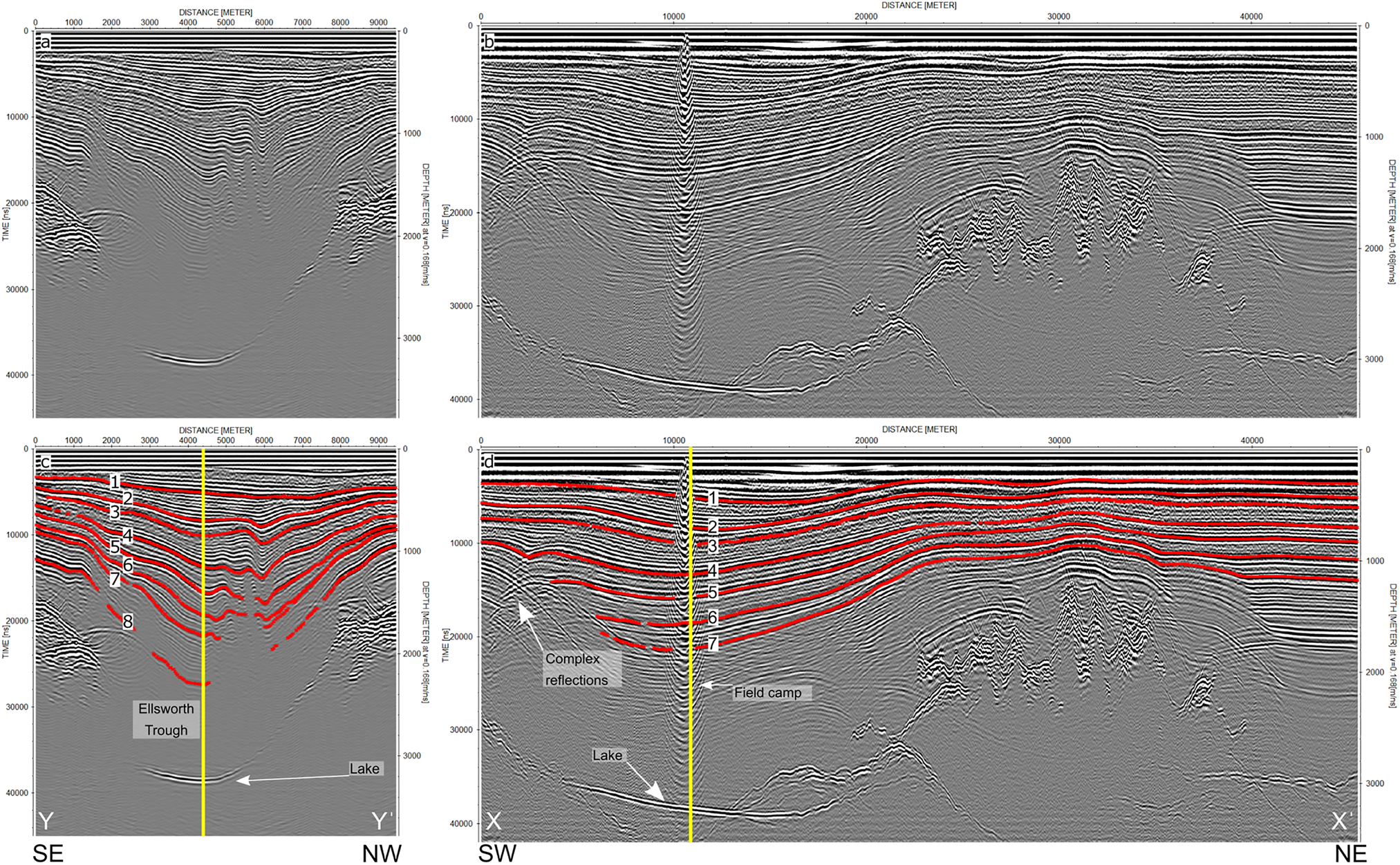
Across ice flow, englacial reflections drape over the rugged topography with traceable layers over the Ellsworth Trough mapped at ice thicknesses up to double that observed over the topographic highs of the valley sidewalls and surrounding highlands and interfluves (Figs 2 and 3). This layer relief (i.e. of up to 1000 m) results in steep englacial layer slopes, which may account for the loss of returned radio-wave power off some of the deeper layers (e.g. layer 8) proximal to the trough's main side walls (Fig. 2c).
Elevation (m WGS84) of gridded englacial layers 1–7 throughout the SLE catchment. (a) ice thickness (m) (from Ross and others, Reference Ross, Siegert, Kennicutt and Bindschadler2011a) with contours at 200 m intervals. Location of RES line D18.25 (Fig. 4a) is shown by a black line; (b) layer 1 elevation; (c) layer 2 elevation; (d) layer 3 elevation; (e) layer 4 elevation; (f) layer 5 elevation; (g) layer 6 elevation; (h) layer 7 elevation. Location of RES line D18.25 (Fig. 4) is shown by a black line. All layers are shown with a common colour scale that is saturated below 400 m WGS84 and above 1600 m WGS84, to demonstrate their evolution with depth through the ice column. All layer elevation contours are at 100 m intervals. The lake shoreline is represented by white (a) and black (b-h) polygons. The orientation of Figures 3a–h has been rotated clockwise by 41.4° for display.
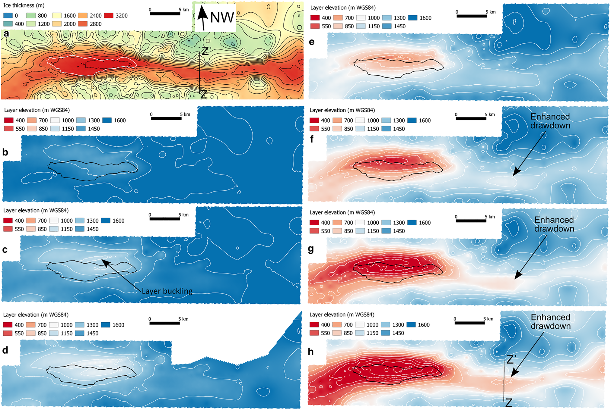
It is apparent from both the radargrams and the gridded DEMs that subglacial topographic relief may not be the only factor influencing englacial form and geometry, however. The maximum drawdown of layers is offset from the centre of the trough axis, with drawdown focused NW of the trough's long axis (e.g. right-hand side of Figs 2a and c). In gridded layers 2–7 the axis of maximum drawdown has a spatial correspondence with the mapped NW lateral edge (i.e. shoreline) of the lake and the NW half of the lake (Fig. 3). This is in direct contrast to the geometry of these layers over the SE side of the lake, where the elevation of all these layers is observed to be rising in the ice located above the lake shoreline (Figs 2a, c and 3). As such, maximum drawdown is offset to the NW of the central axes of both the Ellsworth Trough and SLE.
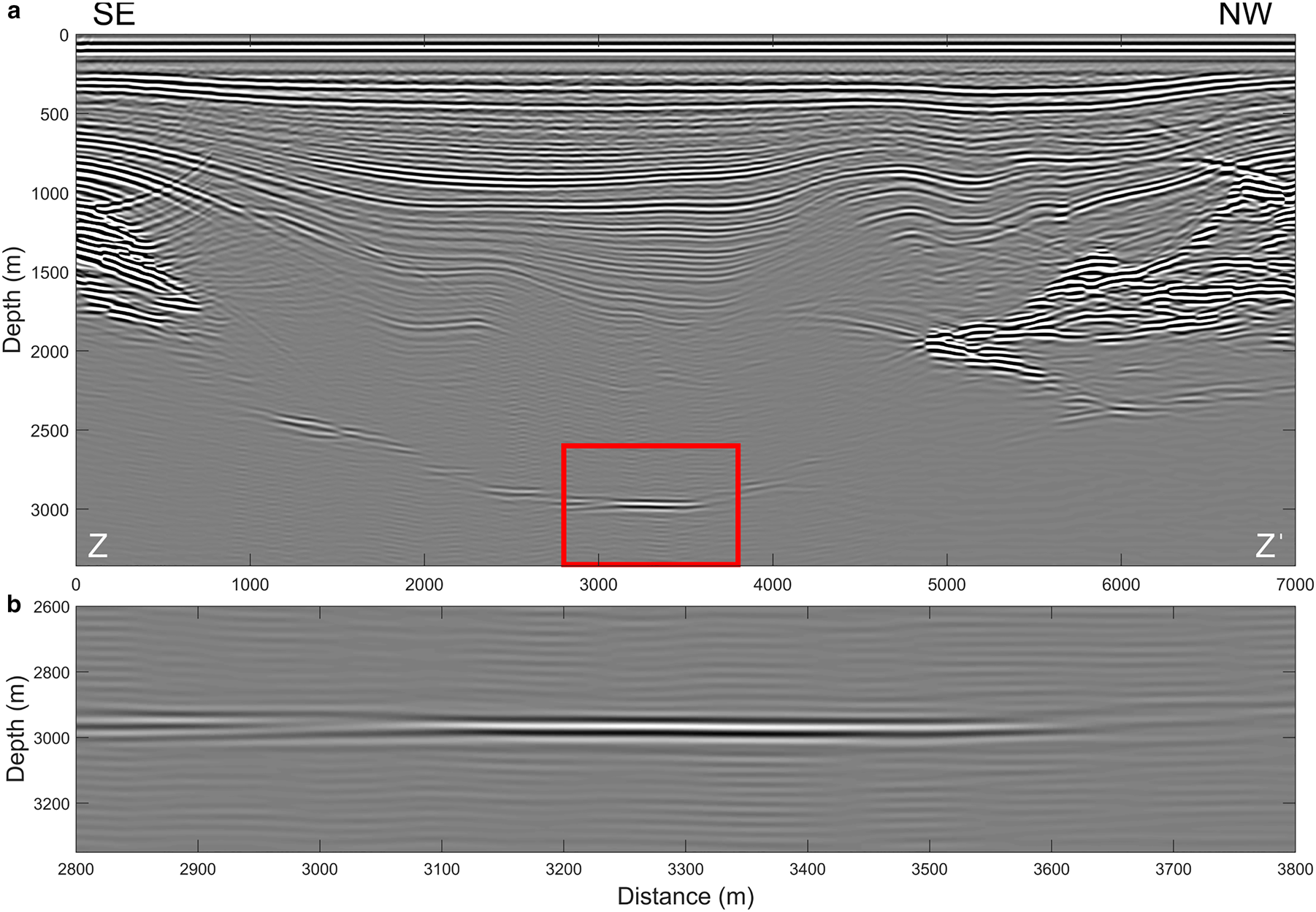
Although there is some sagging of layers throughout the Ellsworth Trough, drawdown is much more pronounced along the length of the lake (Figs 2b, d and 3). In the deeper layers (i.e. layer 4 and below) a second zone of enhanced drawdown is apparent in the base of the Ellsworth Trough between SLE and the ice divide (Figs 3e–h). RES data perpendicular to this zone of layer drawdown are associated with a localised qualitatively bright flat basal reflection in the deepest part of the trough, where the ice is thick (Fig. 3a), directly beneath the maximum layer drawdown (Fig. 4). This is indicative of the presence of a smaller water body in the Ellsworth Trough between SLE and the ice divide (Fig. 4), and is consistent with the potential for a connected subglacial hydrological system along the base of the Ellsworth Trough (Vaughan and others, Reference Vaughan2007; Siegert and others, Reference Siegert2012; Smith and others, Reference Smith2018; Napoleoni and others, Reference Napoleoni2020).
Englacial layer geometry and basal reflection properties associated with a small subglacial water body in the upper Ellsworth Trough. (a) Radargram from survey line D18.25 showing bed topography and englacial layers (see Figs 3a and 3h for location). The red box shows the extent of Figure 4b; (b) zoom-in of radargram D18–25 showing the qualitatively bright flat specular reflection on the floor of the Ellsworth Trough at an ice thickness of nearly 3 km.
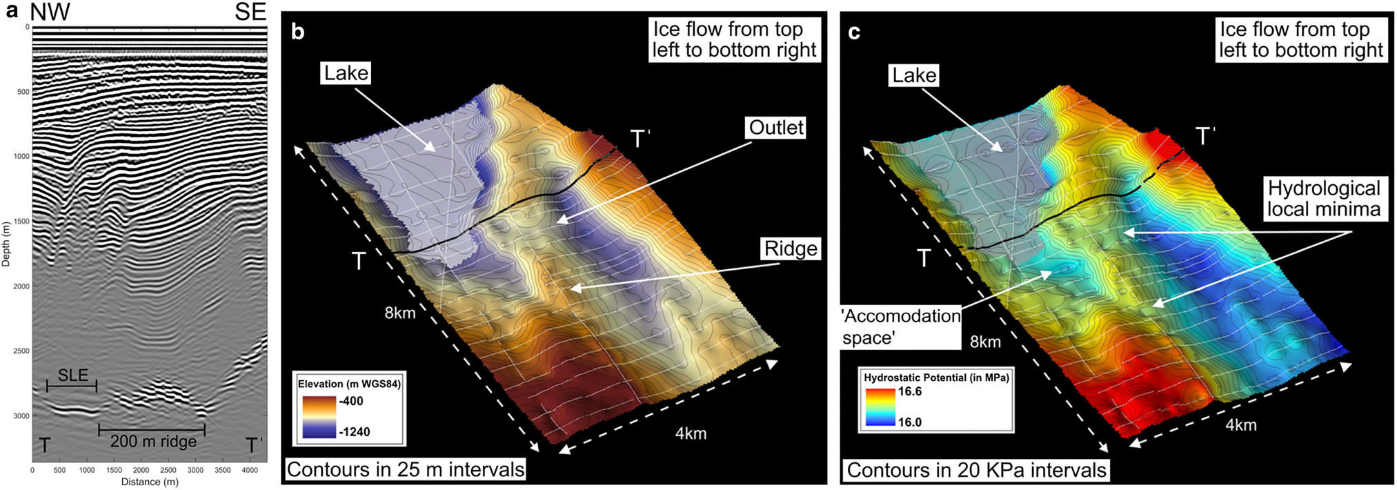
Down-ice of SLE, the englacial layers rise in elevation as the bed rises, and ice flows over a prominent ridge that impounds the bottom end of the lake (Fig. 5) (Siegert and others, Reference Siegert2012; Ross and others, Reference Ross2014; Smith and others, Reference Smith2018). The layer form is also consistent with a transition from sliding to no-sliding associated with the down-ice lake shoreline (Weertman, Reference Weertman1976; Leysinger Vieli and others, Reference Leysinger Vieli, Hindmarsh and Siegert2007). In these ‘down-ice’ parts of the survey area (i.e. SW) englacial reflections are observed nearer to the (on average slightly shallower) bed, with a thinner echo-free zone (Fig. 5a). No evidence for englacial reflections associated with accretion ice (Bell and others, Reference Bell2002) have been observed in any of the DELORES data over and around SLE. The detailed geomorphology of the SLE outlet zone is presented here for the first time (Fig. 5b) and reveals a clear relationship between the 200 m high basal ridge that trends obliquely across the valley, and the down-ice shoreline of SLE. The DEM and hydropotential analysis (Figs 5b and c) also reveals that down-ice of the ridge there is a second smaller basin, and hydropotential low, between the ridge and the SE valley wall. Two possible hydrological connections, associated with low-lying channels that appear to cut across the ridge (Figs 5b and c), may connect SLE with this basin during lake highstands associated with either period of enhanced basal melt, or changes in the steepness of the ice surface (Siegert, Reference Siegert2005). 15–20 km beyond SLE another large subglacial lake has been observed with airborne RES (Vaughan and others, Reference Vaughan2007; Napoleoni and others, Reference Napoleoni2020), and it is possible that episodic connection between SLE and this down-ice lake occurs during such highstands.
High-resolution topography and hydropotential of the outlet zone of SLE. (a) Radargram E2 (for location see 5b and 5c) displaying a narrow bright reflection from the down-ice most part of SLE, and the subglacial topography, including a 200 m high ridge that impounds the down-ice end of the lake; (b) RES-derived DEM of the topography at the outlet of SLE. The lake, its downstream ridge and possible lake outlets are annotated; (c) RES-derived hydropotential map of the outlet zone of SLE, showing the hydropotential high associated with the subglacial ridge. Potential hydrological lows, where water may discharge from SLE, are shown. White lines on 5b and 5c are the location of all DELORES RES data used to produce the topography DEM and the derived hydropotential map. The location of radargram E2 (5a) is represented by a black line. DEM horizontal cell size for 5b and 5c is 50 m. The extents of 5b and 5c are shown in Figure 1a.
5. Discussion
We have demonstrated that the englacial layer drawdown over SLE is focused on the lateral NW shoreline and NW half of the lake. This initially appears to be a surprising finding as, intuitively, we would anticipate basal melting, and therefore englacial layer drawdown, to be focused at the up-ice end of any subglacial lake, where the ice is thickest, and the ice/water interface is lowest. However, processes other than basal melting, such as the Weertman effect (Weertman, 1976; Barcilon and MacAyeal, Reference Barcilon and MacAyeal1993; Leysinger-Vieli and others, Reference Leysinger Vieli, Hindmarsh and Siegert2007) may also play a role in controlling englacial layer form in this case.
GPS observations show that ice flow (Fig. 1b) is slightly oblique to the axis of the Ellsworth Trough (Ross and others, Reference Ross2011b). This means that the ice does not flow straight down the trough, but instead flows north of NE to the south of SW (i.e. obliquely across the trough and the lake). When combined with the elongate and slightly crescent-shaped NW lateral shoreline of SLE, this results in the grounded ice to the NNE of the trough becoming afloat not at the narrow up-ice end of the lake, but instead across a much greater length of shoreline at the NE edge of the lake. Consequently, englacial layer drawdown, possibly associated with lake shoreline melting (Siegert and others, Reference Siegert, Kwok, Mayer and Hubbard2000, Reference Siegert2004; Tikku and others, Reference Tikku2005), is not confined just to the narrow (<1.5 km) up-ice tip of the lake shoreline, as it would be if ice flow was directly along the trough and lake axis, but instead occurs along a shoreline of 5 km.
It is possible that alternative factors may contribute to the geometry of the internal layers over and around the lake. These include the significant relief (>2 km) between the floor of the Ellsworth Trough and the high elevation topography surrounding it, and the shift at the lake shoreline from a no-slip bed to a bed with zero basal resistance (Weertman, 1976). Combined with the oblique ice flow direction, the drawdown of the internal layering may at least partly be a result of mechanical effects of ice flow off the subglacial high and into the deep trough, combined with the ‘Weertman effect’. Disentangling the relative importance of basal melt vs sliding/no-sliding transitions vs mechanical effects with detailed 3-D numerical modelling is beyond the scope of this paper, however. Instead, we assess the vertical and spatial patterns of englacial layer drawdown, comparing our observations with existing numerical models that predict: (a) 3-D flow influences on englacial layering (Leysinger Vieli and others, Reference Leysinger Vieli, Hindmarsh and Siegert2007); and (b) water circulation and basal mass balance within SLE (Woodward and others, Reference Woodward2010; Thoma and others, Reference Thoma2011). We also evaluate the limitations of the SLE englacial layers dataset and discuss the implications of layer drawdown patterns for sediment deposition in the lake.
Despite the 3-D complexity of the ice flow over and around SLE, we suggest that it may be possible to identify the separate effects of both the Weertman effect and basal melt on the SLE layers. There is a substantial drawdown of englacial layers in the upper 50–60% of the ice column (i.e. between layer picks 3–6, Figs 2c and 3d–g) NW of the lake. This layer drawdown may be the result of the transition from no-sliding to sliding as the ice flows over the lake, combined with the impact of ice flow off the high relief subglacial topography (Fig. 1c). In contrast, the greatest amplitude of layer drawdown in layers 7 and 8 (Figs 2c and 3h) is over the NW half of the lake. This SE-ward shift in the maximum amplitude of layer drawdown with ice thickness could be the result of basal melting over the lake becoming the dominant influence on englacial stratigraphy as the ice sheet flows down, and slightly across, the lake. This spatial and vertical pattern of drawdown is consistent with numerical modelling of 3-D layer form (Leysinger Vieli and others, Reference Leysinger Vieli, Hindmarsh and Siegert2007), which suggests that the amplitude of layer drawdown is greater higher up the ice column (in response to sliding) than for the basal melt case (which has greatest drawdown amplitude near to the bed).
The drawdown of the deepest englacial layers over SLE (i.e. layers 7 and 8) has an apparent spatial consistency with the pattern of basal mass balance derived from numerical modelling of water circulation in the lake (Fig. 3 of Woodward and others, Reference Woodward2010). Using an idealised lake geometry, and assuming a closed system, this modelling suggested very high basal melting of 16 cm a−1 in a linear localised zone proximal to the grid-NW side of SLE (Fig. 3 of Woodward and others, Reference Woodward2010). This rate is 2–4 times greater than the melt rate over the centre of the lake, and elsewhere in the up-ice half of the lake. The apparent spatial correspondence between this pattern of modelled melting (Woodward and others, Reference Woodward2010) and the englacial layer drawdown reported here, suggests that the water circulation model produces a relatively realistic representation of the pattern of melting across the lake.
It is important to recognise the limitations of the SLE layers dataset. It is by no means a perfect and comprehensive dataset, and its complexity has potential implications for our ability to confidently evaluate the relative influence of basal melt and changes in basal sliding over the lake. First, englacial layers are only imaged and picked in the radar data for the upper 2/3rds of the ice column (Fig. 2). Numerical modelling (Leysinger Vieli and others, Reference Leysinger Vieli, Hindmarsh and Siegert2007), albeit assuming a flat bed, suggests that the effects of basal melting will cause the largest amplitude of layer drawdown at the base of the ice column, whereas the greatest impact of the Weertman effect will be found in layers at ice thicknesses of ~2/3rds. The radar data do not image layers at depth over SLE, however, limiting their use in identifying zones of basal melt. Second, the SLE radar survey (Fig. 1a) was designed primarily for mapping the extent of the lake and its subglacial hydrological catchment. However, this design was not optimised for characterisation of englacial layering as the survey grid (Fig. 1a) and the ‘along flow’ radar lines (e.g. Fig. 2b) are typically oblique to ice flow (Fig. 1b). The complex relationship between ice flow and the survey lines further complicates our ability to fully disentangle basal melting from the Weertman effect. Third, the englacial structure is further complicated by localised folding caused by ice flow over rugged subglacial topography (Ross and others, Reference Ross2011b) (Fig. 2a). These folds, which track obliquely across the lake, disrupt the radar stratigraphy and make it difficult to confidently pick contiguous stratigraphic layers (Fig. 2c). This is the case even for radar profiles that are oriented closer to ‘along flow’ (e.g. Fig. 2b), due to the oblique tracking of the fold axes (Fig. 2d).
The geometry of the englacial layering, combined with the basal mass-balance output from the water circulation modelling, has potential implications for the pattern and rate of sediment deposition in SLE. The 2-D conceptual models produced to date (Bentley and others, Reference Bentley, Siegert, Kennicutt and Bindschadler2011; Smith and others, Reference Smith2018) have neglected the 3-D implications of layer drawdown along the long grid-NW shoreline of the lake and basal melt being focused on the NW side of the lake. Instead they assume a relatively constant rate of rainout from the ice column across the up-ice parts of the lake, focused on the narrower up-valley (i.e. NE) grounding zone. The englacial layers and the modelling instead point to a possibly more targeted pattern of sediment rainout from the ice base, with the greater flux of sediment likely above the parts of the lake more proximal to the longer grid-NW shoreline. Whether all rained-out sediment is deposited directly without further transport via overflows or underflows in the lake is unknown at present, and is theoretically complicated by the presence of the Line of Maximum Density within the lake (Woodward and others, Reference Woodward2010; Bentley and others, Reference Bentley, Siegert, Kennicutt and Bindschadler2011; Pattyn and others, Reference Pattyn, Carter and Thoma2016). However, we can assume that coarser material will be deposited directly by gravity, meaning that greater rates of sediment deposition are possible beneath the zone of significant englacial layer drawdown and that there is the potential for occasional coarser material to be present nearer to the proposed access location (Woodward and others, Reference Woodward2010) than previously considered. Low acoustic impedance values, indicating a clay- to the silt-rich matrix, dominate the lake floor sediments, however, indicating that fine-grained material is abundant across the lake floor (Smith and others, Reference Smith2018).
The DEM and derived hydropotential of the SLE outlet zone further emphasises the geomorphic and structural geological controls on the location, extent and geometry of SLE (Ross and others, Reference Ross2014), and most likely other subglacial lakes in the Ellsworth Subglacial Highlands (Vaughan and others, Reference Vaughan2007; Rivera and others, Reference Rivera, Uribe, Zamora and Oberreuter2015; Napoleoni and others Reference Napoleoni2020). They also hint at geomorphic evidence for hydrological connections between lakes in the region. It is clear from RES evidence that there is abundant subglacial water within the catchment both up and down ice of SLE (e.g. Fig. 4). As such, hydraulic connectivity, even if only episodic, is a distinct possibility, particularly over glacial-interglacial cycles, when ice divide migration may occur, with potential implications for ice surface slope gradients. Any changes in ice flow configuration (e.g. from ice divide migration over geological timescales) could also lead to variability in the location, rate and pattern of sediment influx and deposition into SLE by altering the distribution and pattern of basal melting. Such changes are unlikely to have occurred over the Holocene, however (Ross and others, Reference Ross2011b). The chemistry of water emanating from melted ice directly over SLE may be different from that sourced from water draining subglacially from the upstream lake (Fig. 4). This is because of the opportunity for solute acquisition during contact with subglacial sediment during the transit of basal water from one lake to the other. This may also vary over time.
One aspect that our current dataset does not allow us to evaluate is the relative importance of basal melt or the input of water into SLE from these subglacial hydrological pathways. However, our study does demonstrate the potential variability in the spatial pattern of basal melting across the lake. If future investigations of subglacial lakes in areas of significant subglacial relief (e.g. Lago CECs or SLE) attempt to determine basal melt rates (e.g. using ApRES), then those investigations cannot assume that basal melt rates will be greatest over the centre of the water body or at the top end of the lake. As such, detailed characterisation of the geometry of englacial layers over target lakes is necessary prior to site selection for measurements of basal melt.
6. Conclusions
1. We characterise the geometry of englacial layers over and around Subglacial Lake Ellsworth (SLE) using low-frequency RES data.
2. Englacial layers are drawn down in a zone that is located along the grid NW shoreline of SLE and over the NW half of the lake.
3. Layer drawdown is interpreted to be the result of (a) the Weertman effect along the length of the ‘grounding line’ of the lake's grid-NW shoreline caused by ice flow oblique to the lake; and (b) a zone of enhanced basal melt above the NW half of the lake. However, we cannot also entirely rule out the influence of mechanical effects associated with significant subglacial relief.
4. The pattern of drawdown inferred from the englacial layers directly over the lake is spatially consistent with basal mass-balance output from a previously published model of water circulation in SLE.
5. Layer drawdown and basal melt over the NW half of the lake has implications for the rate and pattern of sedimentation in SLE and for future measurement and modelling of basal melting over subglacial lakes.
6. Our data do not permit us to determine the relative importance of basal melting compared to inputs from subglacial water. However, the RES data and derived products (e.g. DEMs and maps of hydropotential), do suggest that hydrological connectivity of the cascade of lakes within the Ellsworth Trough is possible, at least episodically. Both direct basal melting (i.e. over the lake), and basal hydrological inputs from the wider catchment will influence physical conditions within SLE.
7. No current evidence exists for the presence of englacial reflections associated with accretion ice over SLE.
Acknowledgements
This work was funded by the Natural Environment Research Council (NERC) Antarctic Funding Initiative (AFI) grants NE/D008751/1, NE/D009200/1, and NE/D008638/1. We thank the British Antarctic Survey for logistics support, NERC Geophysical Equipment Facility for equipment (loans 838, 870), and Dan Fitzgerald and Dave Routledge for excellent fieldwork support. We are grateful to Richard Hindmarsh for productive discussions on the likely processes influencing englacial layer geometry over Subglacial Lake Ellsworth, Ed King for the emergency loan of his DELORES1 radar in the 07/08 field season, and to Hugh Corr and Mark Maltby for the design and build of DELORES2. John Woodward and Andy Smith are thanked for their support, guidance and readings of the poetry of William McGonagall during the 07/08 SLE field season. Knut Christianson (Scientific Editor), Gwendolyn Leysinger Vieli and Elisa Mantelli are thanked for their helpful, supportive and constructive reviews that considerably improved the paper. Aspects of this work were inspired and motivated by the Scientific Committee for Antarctic Research (SCAR) AntArchitecture community.
Shapefiles and gridded surfaces of the picked englacial layers will be made available via the Newcastle University research data repository (https://data.ncl.ac.uk/) in due course.


 Open access

