


Introduction
Normality in statistical analysis refers to the (probability) distribution of a dataset characterized by a symmetric bell-shaped curve, where observations cluster around the mean and taper symmetrically toward both tails (Hair et al., Reference Hair, Black, Babin and Anderson2019, p.48). Normality of the errorFootnote 1 (rather than the raw data; Pek et al., Reference Pek, Wong and Wong2018) is a prerequisite of many statistical analyses, such as the t-test, ANOVA, correlation analyses, and linear regression, which determines the application of parametric methods or nonparametric counterparts (Razali & Wah, Reference Razali and Wah2011; Uhm & Yi, Reference Uhm and Yi2021). Given the significant role of normality, it has attracted great attention from statistical researchers, with over 60 normality checking methods being proposed (Hernandez, Reference Hernandez2021) and new approaches continuing to be developed (e.g., Bayoud, Reference Bayoud2021).
While the diversity of methods provides researchers with various options, it also poses challenges. Normality tests vary significantly in their implementation complexity and reliability. Some are purely descriptive and require a researcher to visually assess whether a distribution follows a bell-shaped curve (e.g., Histogram), but they lack universal criteria for justifying normality (Wijekularathna et al., Reference Wijekularathna, Manage and Scariano2019). In contrast, analytical methods such as Shapiro-Wilk and Kolmogorov-Smirnov tests provide quantified results but can be complex and less intuitive or might not be readily available in some data analysis software (see Yap & Sim, Reference Yap and Sim2011, p. 2142). Furthermore, these methods focus on different aspects of normality, with their sensitivity influenced by the sample size (Kim, Reference Kim2013). Without understanding the underlying logic of normality tests, their differences, and the properties of nonnormality, researchers may struggle to identify which method best aligns with their specific needs.
Research shows that despite the significance and diversity of normality checking methods, researchers in the field of second language (L2) research have paid insufficient attention to this critical assumption (Hu & Plonsky, Reference Hu and Plonsky2021; Lindstromberg, Reference Lindstromberg2016; Plonsky & Ghanbar, Reference Plonsky and Ghanbar2018). Lindstromberg (Reference Lindstromberg2016) reported that only 21 out of 96 quantitative studies reported checking underlying statistical assumptions. Among these, normality was the most frequently tested, yet details about how it was assessed were not always provided. In another synthesis study, Plonsky and Ghanbar (Reference Plonsky and Ghanbar2018) found that only 15.53% L2 studies using multiple regression assessed normality. Hu and Plonsky (Reference Hu and Plonsky2021) further reviewed 107 studies from 2012 to 2017 in Language Learning and Second Language Research that applied analyses requiring normal distribution assumptions (i.e., independent sample t-test (K = 38), one-way ANOVA (K = 42), Pearson correlation (K = 37), multiple regression (K = 17)). Although normality was one of the two most frequently assessed assumptions, it accounted for only 6.7% of all cases. Such a low checking rate is not unique to linguistics but is also true for psychology (Ernst & Albers, Reference Ernst and Albers2017), education (Shatz, Reference Shatz2023), and medical research (Nielsen et al., Reference Nielsen, Nørskov, Lange, Thabane, Wetterslev, Beyersmann, De Unã-Álvarez, Torri, Billot, Putter, Winkel, Gluud and Jakobsen2019). The limited reporting of assumption checking across multiple fields threatens research transparency, which is fundamental to study quality evaluation and reproducibility (Plonsky, Reference Plonsky2024).
While previous systematic reviews have offered valuable insights into how frequently the normality assumption is examined in L2 research, to our knowledge, no L2 study has reviewed the available normality assessment methods or evaluated how accurately these methods are being applied. The present study, rather than reiterating the adequacy of normality checking practices documented in previous research, focuses on the nature of univariate normality. Specifically, we examine common univariate methods for checking normality, including five graphical and seven analytical methods frequently reported in statistical research and available in popular GUI-based (graphical user interface) statistical analysis software or R. We examine how various normality tests function and evaluate their capacity to detect specific forms of deviation from normality, such as skewness, bimodality, and variations in tail heaviness. Moreover, building on Hu and Plonsky’s (Reference Hu and Plonsky2021) work, we broaden the scope from two L2-focused journals to ten Q1 L2-focused journals, and review 237 empirical studies published between 2020 and 2025 that documented normality testing procedures. Rather than calculating the proportion of studies that conducted normality checks, we focus on analyzing the particular tests used, the criteria adopted, and the degree to which researchers followed guidelines recommended by statisticians. We conclude by summarizing common practices currently used in L2 research and suggesting considerations for selecting normality checking methods appropriate to different research contexts.
Literature review
Meaning of univariate normality
Univariate normality refers to the extent to which the distribution of sample data corresponds to a normal distribution, which is typically represented as a bell-shaped curve with data values on the x-axis and their frequencies on the y-axis (Hair et al., Reference Hair, Black, Babin and Anderson2019, p. 48; Thode, Reference Thode2002). Three key features characterize data distribution: asymmetry, tail weight, and peak characteristics (including number and shape), where sample size potentially moderates these properties (Cain et al., Reference Cain, Zhang and Yuan2017). Asymmetry is quantified through skewness, which measures the distribution’s deviation from symmetry around its mean value (Field, Reference Field2018). A distribution with a longer or fatter tail on the left is considered negatively skewed, while one with a longer or fatter tail on the right is positively skewed. Tail weight, referring to the relationship between the central peak and the distribution’s tails, is quantified by kurtosis. Positive kurtosis indicates heavier-than-normal tails on both sides, while negative kurtosis suggests lighter-than-normal tails (Field, Reference Field2018, pp. 344–345). Moreover, the presence of multiple peaks, even when individual peaks exhibit bell-shaped characteristics, can still make the overall distribution deviate from normality and potentially affect statistical analyses (Ventura-León et al., Reference Ventura-León, Peña-Calero and Burga-León2023).
In addition to distribution characteristics, sample size plays a critical role in normality assessment (Hanusz et al., Reference Hanusz, Enomoto, Seo and Koizumi2017; Khatun, Reference Khatun2021). Small samples may pass a normality test with little power, while large samples may flag minor deviation from normality as significantly nonnormal (Öztuna et al., Reference Öztuna, Elhan and Tüccar2006). The Central Limit Theorem (CLT) addresses this challenge by establishing that sampling distributions of means approximate normality as sample size increases, regardless of the underlying population distribution (Altman & Bland, Reference Altman and Bland1995; Kwak & Kim, Reference Kwak and Kim2017). However, debate exists regarding the minimum sample size required for CLT application. Some researchers suggest that the sampling distribution can be assumed normal at K = 30 (Field, Reference Field2018, p. 111; Weinberg & Abramowitz, Reference Weinberg and Abramowitz2002, p. 276), while others recommend continued normality testing and correction for highly skewed data even with samples exceeding 100 (Wilcox, Reference Wilcox2010, pp. 63–85). A more conservative approach suggests that CLT assumptions are appropriate only when samples exceed 200 and the subsequent analyses can accommodate potential normality violations (Demir, Reference Demir2022; Hair et al., Reference Hair, Black, Babin and Anderson2019, p. 219). These considerations highlight the importance of interpreting normality test results in light of sample size.
Significance of normality
Normality is one of the fundamental assumptions underlying parametric inferential statistics (Aryadoust & Raquel, Reference Aryadoust and Raquel2019; Field, Reference Field2018, p. 331; Thode, Reference Thode2002, p. 2). In a perfectly normal distribution, the mean, median, and mode coincide (are equal), and both skewness and “excess kurtosis” are equal to zero (Kim, Reference Kim2013; West et al., Reference West, Finch, Curran and Hoyle1995). Many GUI statistical packages used in L2 research, such as SPSS, Jamovi, and JASP, report excess kurtosis, which is computed by subtracting 3 from the standard kurtosis (kurtosis proper) index (Kim, Reference Kim2013). According to West et al. (Reference West, Finch, Curran and Hoyle1995), the absolute value of kurtosis must be below 7 to avoid substantial deviations from normality, although this threshold refers to standard kurtosis, not excess kurtosis. Excess kurtosis specifically measures the heaviness of the tails of a distribution relative to the normal distribution. A positive excess kurtosis indicates a distribution with heavier tails and a sharper peak, while a negative value suggests lighter tails and a flatter peak. As Kim (Reference Kim2013) notes, an excess kurtosis value substantially above or below zero may indicate that the data are not normally distributed and could affect the robustness of parametric statistical analyses that assume normality.
Although nonparametric alternatives are available for situations where the assumption of normality is violated, these methods generally have lower statistical power than their parametric counterparts when applied to data that are normally distributed (Keren & Lewis, Reference Keren and Lewis2014). Therefore, it may not always be appropriate to default to nonparametric tests to avoid normality testing (Le Cessie et al., Reference Le Cessie, Goeman and Dekkers2020; Parsons et al., Reference Parsons, Price, Hiskens, Achten and Costa2012). Instead, for moderately nonnormal datasets, correction or transformation methods should be employed to fit parametric analyses (Pek et al., Reference Pek, Wong and Wong2018). For example, in their review of 61 statistics textbooks, Pek et al. (Reference Pek, Wong and Wong2018) identified a range of recommended strategies for addressing nonnormality, including data transformations, heteroscedasticity-consistent standard errors, bootstrap-based methods, and likelihood-based adjustments. Among these, power transformations—such as the Box-Cox and Yeo-Johnson transformations—are commonly applied to stabilize variance and improve the approximation to normality, particularly when moderate skewness or kurtosis is present (Raymaekers & Rousseeuw, Reference Raymaekers and Rousseeuw2024). More recent contributions, such as those by Raymaekers and Rousseeuw (Reference Raymaekers and Rousseeuw2024), have proposed robust methods for estimating transformation parameters in the presence of outliers, which help preserve the central tendency of the data without unduly distorting its tails.
The importance of normality extends beyond the choice between parametric and nonparametric analyses (Vrbin, Reference Vrbin2022). It influences parameter estimation, confidence intervals, and hypothesis testing (Field, Reference Field2018, p. 331). A recent study by Ventura-León et al. (Reference Ventura-León, Peña-Calero and Burga-León2023) demonstrated how various nonnormal distributions affect correlation coefficient estimation. They investigated bimodal nonnormality (with outliers at means of 3 or 6), distributions with varying degrees of skewness (0 to 2.5), and kurtosis (–1.39 to 25), analyzing their impact on Pearson, Spearman, and Pearson Winsorized correlation coefficients (a robust version of the Pearson correlation designed to reduce the influence of outliers) across sample sizes (between 50 and 1000). Their findings revealed large discrepancies in bimodal distributions with outliers (mean = 6) for Spearman coefficients across all sample sizes (Ventura-León et al., Reference Ventura-León, Peña-Calero and Burga-León2023, p. 414). Although this study did not examine highly skewed distributions, which limits its representation of nonnormality, it illustrates two critical aspects of normality. On the one hand, it demonstrates how certain types of departure from normality can significantly affect statistical outcomes, which supports the premise that the validity of inferential results depends on how well data approximate a normal distribution (Uhm & Yi, 2023). On the other hand, it shows that not all departures from normality can substantially impact statistical analyses, as some non-normal distributions produce no noticeable differences in coefficient estimates (Ventura-León et al., Reference Ventura-León, Peña-Calero and Burga-León2023). It aligns with previous findings that suggest some statistical approaches can effectively handle moderate normality violations, particularly with adequate sample sizes (Cain et al., Reference Cain, Zhang and Yuan2017; Knief & Forstmeier, Reference Knief and Forstmeier2021). For example, in very large samples, it is often unnecessary for the errors of the general linear model (e.g., ANOVA and linear regression) to follow a strictly normal distribution due to the CLT. As Pek et al. (Reference Pek, Wong and Wong2018, p. 4) explained:
[r]egardless of the distribution of ε [errors in the general linear model], the CLT assures that the sampling distribution of the estimates will converge toward a normal distribution as N increases to infinity, when ε are independent and identically distributed, and when σ2 is finite.
Thus, for sufficiently large samples, the sampling distribution of parameter estimates tends to be normal even if the error terms themselves are not, thereby preserving the validity of inferential tests under standard linear modeling frameworks.
These findings suggest that while normality is a crucial statistical assumption that could influence statistical validity, it should not be treated as a binary criterion for choosing between parametric and nonparametric analyses, nor should deviation from perfect normality be regarded as an “evil” that necessarily leads to bias in parameter estimations (Knief & Forstmeier, Reference Knief and Forstmeier2021). Moreover, it is important to understand the nature of the data and the underlying nature of the test. For instance, the correlations mentioned above can only detect monotone tendencies, meaning that they may fail to reveal the true relationship if the data are entrenched with nonmonotone tendencies; for such cases, more recent correlation alternatives can be used (Chatterjee, Reference Chatterjee2021) to reveal the true relationship regardless of the distribution of the data. Although a comprehensive discussion of these considerations extends beyond our study’s scope, the severity of normality violations and the robustness of analytical methods to such violations are factors that may inform how results are interpreted and whether alternative analyses are appropriate. This context underscores the importance of our study, which investigates the functioning and sensitivity of various normality tests in detecting different forms of nonnormality. The analysis provides insight into how these tests operate and the implications of their outcomes for subsequent statistical procedures.
Univariate normality tests
Given the significant role of normality in statistics, researchers have proposed over 60 normality assessment approaches (Hernandez, Reference Hernandez2021, pp. 3–11), which can be categorized into graphical methods, tests based on the empirical cumulative distribution function (ECDF), tests based on regression and correlation (especially using order statistics), tests based on moments (such as skewness and kurtosis), and a range of other analytical methods (see Table 1). These five categories can be broadly grouped into two overarching types: graphical methods and analytical tests (Field, Reference Field2018; Hair et al., Reference Hair, Black, Babin and Anderson2019).
Overview of 61 normality tests categorized by methodological type and primary references presented by Hernandez (Reference Hernandez2021, pp. 3–11)

Table 1. Long description
The table is organized into two columns: Test abbreviation and Test name and category. It is divided into five methodological sections:
1. Graphical method: H I S T (Histogram), S T E M (Stem-and-leaf Plot), B O X (Box-and-whisker Plot), C D F (Cumulative Distribution Function Plot), P P P (P-P Plot), and Q Q P (Q-Q Plot).
2. Empirical cumulative distribution function: A D (Anderson-Darling), K S (Kolmogorov-Smirnov), L F (Lilliefors), C V M (Cramer-von Mises), W A (Watson), A J N (Ajne), Z A (Zhang-Wu Z A), K U (Kuiper), G L B (Glen-Leemis-Barr), Z C (Zhang-Wu Z C), F R O (Frosini), G T (G Test), and N D (N-distanceleft).
3. Moments: H L M (Hosking L-moments), B H S B S (Brys-Hubert-Struyf-Bonett-Seier), A J B (Adjusted Jarque-Bera), J B (Jarque-Bera), P D A B (Pearson-D’Agostino-Bowman), D A K (D’Agostino-Pearson Kurtosis), D A P (D’Agostino-Pearson K 2), B S (Bonett-Seier), D A S (D’Agostino-Pearson Skewness), D L (Desgagné-Lafaye), D H (Doornik-Hansen), R J B (Robust Jarque-Bera), B M (Bontemps-Meddahi), D D L (Directional Desgagné-Lafaye), B H S (Brys–Hubert–Struyf), C C K (Cabaña-Cabaña Kurtosis), T L M (Trimmed L-moments), and C C S (Cabaña-Cabaña Skewness).
4. Regression and correlation: S W (Shapiro-Wilk), S F (Shapiro-Francia), C S (Chen-Shapiro), C O (Coin), W B (Weisberg-Bingham), R G (Rahman-Govindarajulu), F B (Filliben), H G 2 (Hegazy-Green 2), R J (Ryan-Joiner), R O Y (Royston), D A D (D’Agostino D), B C M R (del Barrio-Cuesta-Matrán-Rodríguez), Z H (Zhang), G K 0 (Gan-Koehler k 0), G K (Gan-Koehler k 2), D W V (De Wet-Venter), and H G 1 (Hegazy-Green 1).
5. Others: V A (Vasicek), G M G (Gel-Miao-Gastwirth), C H I super 2 (Chi-squared), G E (Geary), E P (Epps-Pulley), S H (Spiegelhalter), and M I (Martinez–Iglewicz).
* Although the Chi-squared (Chi2/χ2) test can be configured to assess normality, it is a general goodness-of-fit procedure rather than a test specifically designed for this purpose. Its performance depends strongly on how class intervals are defined and on sample size, which limits its usefulness for evaluating normality in some applications. Thus, despite Hernandez (Reference Hernandez2021, pp. 3–11) mentioning it among normality tests, we consider it tangentially relevant to normality assessment.
Extensive research has been conducted to identify the “best” analytical normality tests across diverse distributions and sample sizes (e.g., Arnastauskaitė et al., Reference Arnastauskaitė, Ruzgas and Bražėnas2021; Patrício et al., Reference Patrício, Ferreira, Oliveiros and Caramelo2017; Thode, Reference Thode2002). In the comprehensive review summarized in Table 1, Hernandez (Reference Hernandez2021) analyzed the statistical power of 55 analytical normality tests and identified the Shapiro-Wilk (SW) test as the most frequently used and effective approach. However, this conclusion needs careful interpretation. First, as Hernandez (Reference Hernandez2021) noted, the high ranking of the SW test may be attributed to its frequent inclusion in these studies. Second, test performance varies with dataset characteristics, which can be influenced by sample size and distribution type (Nosakhare & Bright, Reference Nosakhare and Bright2017; Wijekularathna et al., Reference Wijekularathna, Manage and Scariano2019). Thus, combining or averaging results from studies that differ in distributional characteristics and sample sizes may lead to potentially misleading conclusions.
Current comparative studies typically evaluate numerous normality tests (e.g., Arnastauskaitė et al., Reference Arnastauskaitė, Ruzgas and Bražėnas2021, evaluating 31 tests) across multiple non-normal distributions (e.g., Jiménez-Gamero, Reference Jiménez-Gamero2023, evaluating 12 distributions). While existing studies provide valuable insights into the performance of normality tests under various conditions, opportunities remain to extend this work. Most studies focus on reporting test statistics and distribution parameters. This could be complemented by a deeper examination of the underlying principles and how specific distributional characteristics influence test performance. Some researchers have begun categorizing non-normal distributions based on features such as tail weights (Jelito & Pitera, Reference Jelito and Pitera2021) or symmetry (Uhm & Yi, Reference Uhm and Yi2021), which opens promising avenues for more systematic investigation. Building on these foundations, a clearer understanding of distributional characteristics and test sensitivities would help L2 researchers and practitioners make more informed choices when selecting suitable normality tests. Additionally, although graphical normality tests present interpretive challenges (Wijekularathna et al., Reference Wijekularathna, Manage and Scariano2019), they remain an underexplored aspect of normality assessment and could be used alongside quantitative methods to provide a more complete understanding of distributional characteristics.
To address these limitations, we examine both graphical and frequently used analytical normality tests, where we explain their underlying mechanisms. We selected analytical tests based on Hernandez’s (Reference Hernandez2021) and Thode’s (Reference Thode2002) studies, focusing on those appearing in more than 10 out of 20 studies, including Shapiro-Wilk (SW), Shapiro-Francia (SF), Kolmogorov-Smirnov (KS), Lilliefors, Cramer-von Mises (CVM), Anderson-Darling (AD), and Jarque-Bera (JB), alongside skewness and kurtosis measures.
Graphical measures
Graphical measures for assessing normality can be categorized into two main approaches: those based on raw data or frequency visualization such as Histograms, and those employing goodness-of-fit (GoF) principles to compare sample distributions against theoretical normal distributions such as quantile-quantile (Q-Q) plots (Thode, Reference Thode2002).
Raw-data-based graphical approaches. Raw-data-based methods comprise three commonly used approaches: Histograms, Stem-and-leaf plots (Tukey, Reference Tukey1977), and boxplots (box-and-whisker plots) (Tukey, Reference Tukey1977).
Histograms. Histograms display frequency distributions by grouping values into contiguous intervals, or bins, along the x-axis, with corresponding bars representing the frequency of observations on the y-axis. This visual method enables a quick assessment of the distribution’s shape, including its symmetry, skewness, modality, and potential outliers. A bell-shaped histogram suggests normality, whereas noticeable skew, flatness, or multiple peaks may indicate deviations from a normal distribution. Although histograms can be applied to datasets of various sizes, their interpretability is highly sensitive to bin width, which can either obscure or exaggerate distributional features if not appropriately chosen (Correll et al., Reference Correll, Li, Kindlmann and Scheidegger2019; Indira et al., Reference Indira, Vasanthakumari, Sakthivel and Sugumaran2011). As such, histograms tend to produce more stable and informative visualizations with larger samples, typically when the sample size reaches approximately 200 or more observations (Neter et al., Reference Neter, Kutner, Nachtsheim and Wasserman2005; Oppong & Agbedra, Reference Oppong and Agbedra2016).
Stem-and-leaf plots. Stem-and-leaf plots offer a more detailed visualization by organizing individual data points as “leaves” attached to categorical “stems.” Unlike histograms that represent frequency through bar height, this method preserves and displays individual values, which enables more granular data examination (Oppong & Agbedra, Reference Oppong and Agbedra2016). The distribution’s shape can be interpreted by observing the symmetry of the leaves around the center; a roughly symmetric spread suggests normality, while a concentration of leaves on one side indicates skewness. Gaps or clusters may reveal data irregularities, and repeated values are easily spotted. This makes stem-and-leaf plots particularly useful for identifying patterns, outliers, and the central tendency in small to moderately sized datasets. However, its readability decreases with larger datasets and may remove data points to maintain clarity (Ajao et al., Reference Ajao, Obafemi and Bolarinwa2018).
Boxplots. Boxplots (box-and-whisker plots), which also utilize raw data, summarize data dispersion through a combination of box and whiskers. They display the mean, quartiles, range, and potential outliers, which is effective for dataset comparison (Mishra et al., Reference Mishra, Pandey, Singh, Gupta, Sahu and Keshri2019). However, because boxplots visualize summarized data using five key statistics (minimum, quartile 1 (Q1), median, quartile 3 (Q3), maximum) rather than individual data points, they can hardly show specific distribution or frequency information of the dataset (see Figure 1)—a quartile divides an ordered dataset into four equal parts, each containing 25% of the data. Moreover, their utility may be limited with small datasets, where single outliers can disproportionately influence quartiles calculation and whiskers position, and potentially distort the perceived distribution (Ahmadiyeh et al., Reference Ahmadiyeh, Sajedi-Amin, Kafili-Hajlari and Naseri2023).
A representation of a Boxplot.

Figure 1. Long description
A vertical axis on the left is labeled Variable with numerical increments from 25 to 70. The boxplot consists of the following elements from top to bottom.
* Maximum: A red horizontal line at the top of a dashed whisker, labeled Maximum (Q 3 + 1.5 times I Q R).
* Upper Quartile: The top edge of the blue box, labeled Q 3 (75th percentile) Upper Quartile.
* Median: A green horizontal line bisecting the blue box, labeled Median (50th percentile) Middle value.
* Lower Quartile: The bottom edge of the blue box, labeled Q 1 (25th percentile) Lower Quartile.
* Interquartile Range: A purple vertical bracket spanning the height of the blue box, labeled I Q R Interquartile Range.
* Minimum: A red horizontal line at the bottom of a dashed whisker, labeled Minimum (Q 1 - 1.5 times I Q R).
* Outlier: A single red dot located below the minimum whisker, labeled Outlier Beyond whiskers.
Figure 1 presents a labeled boxplot, which is a graphical method for visualizing the distribution, central tendency, and spread of a continuous variable. The box in the center represents the interquartile range (IQR), which spans from the first quartile (Q1, 25th percentile) to the third quartile (Q3, 75th percentile). This range captures the middle 50% of the data. The thick horizontal line inside the box marks the median (50th percentile), indicating the central value of the distribution. Whiskers extend from either end of the box to the smallest and largest values within 1.5 times the IQR below Q1 and above Q3, respectively. Any data points that fall outside this range are plotted individually and considered outliers. One can infer the skewness of the distribution by examining the symmetry of the box and the length of the whiskers. A perfectly symmetric box with equal-length whiskers suggests normality, whereas noticeable asymmetry indicates skew. The presence and number of outliers provide additional insight into the variability and potential anomalies in the data.
However, boxplots are less capable of dealing with bimodal distributions. Choonpradub and McNeil (Reference Choonpradub and McNeil2005) discussed in detail how a boxplot could look the same as that of a normal distribution when the raw data actually follows a perfectly symmetric bimodal distribution (a set of data that has two main peaks or high points), meaning that it could mask the real distribution shown in a histogram.
Goodness-of-fit (GoF)-based graphical approaches. Unlike raw-data approaches that visualize data distribution directly, GoF-based measures, like P-P plots and Q-Q plots, compare sample distributions against their theoretical normal counterparts.
Probability-Probability (P-P) plots. P-P plots compare the theoretical cumulative probability function (CDF) of a variable with the ECDF (Rani Das, Reference Rani Das2016). These plots display theoretical cumulative probabilities on the x-axis against empirical cumulative probabilities on the y-axis, with a diagonal line indicating perfect alignment with the normal distribution. The cumulative nature of P-P plots makes them particularly sensitive to central distribution deviations (Delignette-Muller & Dutang, Reference Delignette-Muller and Dutang2015; Wilk & Gnanadesikan, Reference Wilk and Gnanadesikan1968). Minor deviations in the central region produce notable divergences from the diagonal reference line, while tail deviations may be less apparent due to the cumulative calculation diluting outlier effects (see Figure 2A).
P-P plot (A) and Q-Q plot (B) with 20 unexpected values.

Figure 2. Long description
A two-panel vertical layout.
Panel A is titled P P Plot. The x-axis is Theoretical C D F (Normal Distribution) ranging from 0.0 to 1.0. The y-axis is Empirical C D F ranging from 0.0 to 1.0. A red diagonal reference line runs from the bottom-left to the top-right. Blue data points follow a slightly curved path below the red line. A small cluster of green points appears between 0.6 and 0.7 on the x-axis. At the far right, a vertical stack of red open circles is located at x equals 1.0, ranging from y equals 0.9 to 1.0.
Panel B is titled Q Q Plot. The x-axis is Theoretical Quantiles ranging from approximately 20 to 80. The y-axis is Sample Quantiles ranging from 40 to 100. A red diagonal reference line bisects the chart. Blue data points form an S-shaped curve that crosses the red line. A small cluster of green points is located near the center at x equals 55. In the top-right quadrant, a distinct horizontal cluster of red solid points is positioned significantly above the diagonal line, ranging from x equals 65 to 80 at a y-value of approximately 100.
Quantile-Quantile (Q-Q) plots. Q-Q plots also employ a diagonal line to indicate perfect normality but utilize quantile comparisons rather than cumulative probabilities. A quantile is a point that divides a dataset (or a theoretical distribution) into equal-sized portions. Theoretical quantiles (calculated using an inverse normal function) are plotted on the x-axis against empirical quantiles on the y-axis (Wilk & Gnanadesikan, Reference Wilk and Gnanadesikan1968). This approach excels at revealing tail behaviors in data distributions but may be less informative about central tendencies, which often appear as a straight line (see Figure 2B), particularly in large samples (Ajao et al., Reference Ajao, Obafemi and Bolarinwa2018; Rodu & Kafadar, Reference Rodu and Kafadar2022).
Figure 2 demonstrates the complementary strengths of these GoF-based graphical approaches using a dataset with both tail anomalous values (red dots, mean = 100, SD = 2) and upper middle anomalous values (green dots, mean = 55, SD = 2). The P-P plot effectively highlights central distribution anomalies (green dots), while the Q-Q plot clearly reveals tail deviations (red dots) through marked departures from the diagonal line. This comparison illustrates how P-P plots excel at detecting central distribution deviations while Q-Q plots are more effective in identifying tail anomalies (Gan & Koehler, Reference Gan and Koehler1990).
Analytical measures
While graphical methods offer intuitive visualization and are widely available in commonly used statistical software in L2 research including SPSS, Jamovi, JASP, and R, as demonstrated in Table 2, their subjective interpretation may not be sufficient for normality assessment (Henderson, Reference Henderson2006). Therefore, analytical measures are indispensable and should be interpreted alongside graphical tests to validate statistical analysis choices (Keselman et al., Reference Keselman, Othman and Wilcox2013; Öztuna et al., Reference Öztuna, Elhan and Tüccar2006). As demonstrated in Figure 3, analytical tests can be categorized into moment-based (e.g., Jarque-Bera test) and GoF-based tests, with the latter further divided into empirical distribution function-based measures (e.g., Kolmogorov-Smirnov test) and regression/correlation-based measures (e.g., Shapiro-Wilk test) (Hernandez, Reference Hernandez2021; Marange & Qin, Reference Marange and Qin2021). These analytical methods will be discussed next.
An overview of graphical and analytical methods for assessing normality and their availability in common statistical packages (as of November 2025)

Table 2. Long description
The table is divided into two primary sections: Graphical and Analytical methods.
Graphical methods include:
- Raw data plotting: Histogram, Stem-and-leaf plots, and Boxplots. All are available in S P S S, J A S P, and R. Jamovi lacks Stem-and-leaf plots.
- Goodness-of-fit plotting: P-P plot and Q-Q plot. Q-Q plots are available in all packages. P-P plots are available in S P S S, J A S P, and R, but require R-based modules in Jamovi.
Analytical methods include:
- Moment-based: Skewness and Kurtosis are available in all packages. The Jarque-Bera J B test is available in S P S S and R only.
- Empirical distribution function-based: Kolmogorov-Smirnov K S and Anderson-Darling A D tests are available in all packages. Lilliefors and Cramer-von Mises C V M tests are available in S P S S and R, with C V M also available in J A S P.
- Regression or correlation-based: Shapiro-Wilk S W test is available in all packages. Shapiro-Francia S F test is available in S P S S and R only.
Footnotes indicate S P S S data is based on version 30 plus and Jamovi P-P plots require the R j editor or specific community modules.
* The SPSS functions described are based on version 30+. Some features may not be available in earlier versions.
** As of November 2025, Jamovi does not natively generate P-P plots. They can be created via the Rj editor using R packages such as ggplot2, car, or ggpubr. In addition, some community modules in the Jamovi library (for example, GAMLj or Rj) allow users to run R code that includes P-P plot generation.
Classification of analytical normality tests by methodological approach.

Figure 3. Long description
A hierarchical flowchart with three levels of classification.
At the top level is a single box labeled analytical normality tests.
From this root, two arrows point down to the second level.
1. The left branch leads to moment-based tests.
2. The right branch leads to goodness of fit G O F-based tests.
Under the moment-based branch, two arrows point to a third level containing skewness and kurtosis. These two boxes then converge with arrows pointing to a final box labeled Jarque-Bera J B test.
Under the goodness of fit G O F-based branch, two arrows point to a third level.
1. The left sub-branch is empirical distribution function E D F-based. This further divides into two boxes: Kolmogorov-Smirnov K S and Lilliefors test, and Cramer Von Mises C V M and Anderson-Darling A D test.
2. The right sub-branch is correlation or regression-based. This leads to a single box labeled Shapiro-Wilk S W and Shapiro-Francia S F test.
In reviewing analytical normality test formulas, it is important to note that variations exist between sample-based and population-based calculations (Doane & Seward, Reference Doane and Seward2011). This study focuses on sample-based formulas for two reasons. First, sample-based formulas explicitly incorporate the sample size of the study, which is useful in understanding why normality tests are sensitive to sample sizes. Second, there is a practical consideration that most, if not all, statistical software packages use sample-based rather than population-based normality tests. Understanding sample-based formulas therefore helps researchers better interpret the results their software produces.
Moment-based methods of assessing normality. Moment-based methods of assessing normality evaluate the shape of a distribution using its statistical moments—particularly the third and fourth central moments—to assess deviations from normality (Thode, Reference Thode2002). As previously discussed, skewness, derived from the third moment, measures asymmetry, indicating whether values lean to the left or right of the mean. Kurtosis, based on the fourth moment, quantifies the heaviness of the distribution’s tails and the sharpness of its peak. The Jarque-Bera (JB) test integrates these two metrics into a single goodness-of-fit measure by computing a test statistic using sample skewness and kurtosis to assess normality (Jarque & Bera, Reference Jarque and Bera1987; Thadewald & Büning, Reference Thadewald and Büning2007). These methods are discussed next.
Skewness. Skewness is a descriptive statistic measure that quantifies the degree of asymmetry in a probability distribution around its mean (Doane & Seward, Reference Doane and Seward2011; Ho & Yu, Reference Ho and Yu2015). It is calculated using the third moment of the mean and standardized by the cube of the SD:

where n is the sample size,
$ {X}_i $
 is each data point,
$ \overline{X} $
is each data point,
$ \overline{X} $
 the mean of the data and
$ SD $
the mean of the data and
$ SD $
 the standard deviation (DeCarlo, Reference DeCarlo1997). In a perfectly normal distribution, skewness equals zero, while the mean equals the sample’s median and mode (Hatem et al., Reference Hatem, Zeidan, Goossens and Moreira2022). The cubic power in the formula intensifies the influence of values far from the mean, making it sensitive to outliers at the tails and amplifying the direction of the tails (Doane & Seward, Reference Doane and Seward2011). A positively skewed distribution features a long tail on the right with fewer large values, whereas a negatively skewed distribution shows a concentration of data on the right with a tail extending to the left (Hair et al., Reference Hair, Black, Babin and Anderson2019).
The interpretation of skewness values is influenced by sample size (Kim, Reference Kim2013). To standardize skewness across different sample sizes and make it comparable, Z-scores, which account for the standard error of skewness, are recommended when dealing with small samples. The Z-score is computed by dividing the skewness (or kurtosis) values by their standard errors (Tabachnick & Fidell, Reference Tabachnick and Fidell2013). For small samples (n < 50), the significant deviations are typically assessed against a critical Z-value of ±1.96 at an alpha level of 0.05. For medium-sized samples (50 < n <300), significant deviations are usually assessed against a critical Z-value of ±3.29. For large samples (n > 300), an absolute skewness value greater than 2 might suggest nonnormality (Kim, Reference Kim2013). On the other hand, according to Mayers (Reference Mayers2013), for sample sizes between 50 and 175, a more stringent critical value of ±2.58, which corresponds to a 1% significance level (p < 0.01), is appropriate for z-scores of skewness and kurtosis, rather than the conventional ±1.96 (corresponding to p = .05). Proposed absolute skewness thresholds for normality assessment vary considerably in the literature, ranging from conservative values of 0.5 (Hatem et al., Reference Hatem, Zeidan, Goossens and Moreira2022) to more lenient thresholds of 1.5 (George & Mallery, Reference George and Mallery2001) and 3 (Kline, Reference Kline2016).
Kurtosis. Kurtosis is another moment-based measure that is calculated as the standardized fourth moment about the mean:

where n is the sample size,
$ {x}_i $
 denotes each observation value,
$ \overline{x} $
denotes each observation value,
$ \overline{x} $
 is the sample mean, and
$ SD $
is the sample mean, and
$ SD $
 is the sample mean, and
$ SD $
is the sample mean, and
$ SD $
 is the sample standard deviation (Cain et al., Reference Cain, Zhang and Yuan2017; DeCarlo, Reference DeCarlo1997). While commonly misinterpreted as merely reflecting distribution peak height, with positive kurtosis indicating a higher peak and negative kurtosis a lower peak, kurtosis characterizes both tail weight and peak characteristics of the data distribution (Balanda & MacGillivray, Reference Balanda and MacGillivray1988). As discussed earlier, a normal distribution has an excess kurtosis of 0 (excess Kurtosis = Kurtosis proper – 3), representing balanced tail weights (Hair et al., Reference Hair, Black, Babin and Anderson2019). Distributions with positive excess kurtosis display both increased peak height and heavier tails, indicating a higher probability of extreme values compared to a normal distribution. Conversely, negative excess kurtosis manifests as both a flatter peak and lighter tails, reflecting fewer extreme values.
Like skewness, the interpretation of kurtosis depends on sample size. While Kline (Reference Kline2016) proposed a general threshold of ±10, other researchers advocate for sample size-dependent criteria. Large samples usually provide more reliable excess kurtosis estimates. For small samples, where outliers can disproportionately affect the measure, Kim (Reference Kim2013) recommended using Z-score: ±1.96 for samples smaller than 50, and ±3.29 for sample sizes ranging from 50 to 300 (Kim, Reference Kim2013). Mayers (Reference Mayers2013) further refined these guidelines to suggest a Z-score range of ±2.58 for sample sizes between 50 and 175.
Jarque-Bera (JB) test. Although skewness and kurtosis are critical measures for distributional properties, neither measure alone comprehensively captures all features of normality (Kim, Reference Kim2021). To synthesize both skewness and kurtosis, Jarque and Bera (Reference Jarque and Bera1987) proposed the JB test as follows:

where n is the sample size. Under the null hypothesis of normality, the JB value, which combines both skewness and excess kurtosis, should theoretically converge to zero. This statistic follows a chi-squared distribution with two degrees of freedom, where a larger JB value indicates a stronger deviation from normality. The null hypothesis is rejected when the JB statistic exceeds the critical value derived from the chi-squared distribution (Kim, Reference Kim2021; Thadewald & Büning, Reference Thadewald and Büning2007). For example, at a significance level of 0.05, the critical value from the chi-squared distribution with two degrees of freedom is approximately 5.99. If the computed JB statistic exceeds this threshold, the data is considered nonnormally distributed. Conversely, a JB statistic below this critical value suggests insufficient evidence to reject the assumption of normality. As an integration of skewness and kurtosis, this test is also sensitive to sample size (Demir, Reference Demir2022) and has multiple criteria to interpret the results (see Wijekularathna et al., Reference Wijekularathna, Manage and Scariano2019), but it is particularly useful in large samples, where its asymptotic properties yield reliable results.
Goodness-of-fit (GoF)-based measures. GoF-based measures complement moment-based approaches in normality testing by comparing observed data distributions with theoretical normal distributions through various computational methods, such as empirical distribution function (EDF)-based measures and correlations/regressions (Marange & Qin, Reference Marange and Qin2021). GoF methods for assessing normality include the Kolmogorov-Smirnov test, Lilliefors test, Cramér-von Mises test, Anderson-Darling test, Shapiro-Wilk test, and Shapiro-Francia test, all of which are discussed in the following sections.
Kolmogorov-Smirnov (KS) test. The KS test quantifies the maximum discrepancy between the EDF of the data and the CDF of a normal distribution, expressed as:

where sup denotes the maximum difference over all possible values,
$ {F}_n(x) $
 represents the empirical distribution function of the data and
$ F(x) $
is the theoretical CDF (Armitage & Colton, Reference Armitage and Colton1998).
represents the empirical distribution function of the data and
$ F(x) $
is the theoretical CDF (Armitage & Colton, Reference Armitage and Colton1998).
This test does not assume the data must follow any specific parametric distribution, which allows for its application across any continuous distribution (Kim, Reference Kim2013). However, this flexibility comes at the cost of reduced efficiency and power compared to other normality tests (Arnastauskaitė et al., Reference Arnastauskaitė, Ruzgas and Bražėnas2021; Emmanuel et al., Reference Emmanuel, T. Maureen and Wonu2020; Steinskog et al., Reference Steinskog, Tjøstheim and Kvamstø2007). Although it demonstrates improved performance with larger datasets (Keselman et al., Reference Keselman, Othman and Wilcox2013), the test becomes overly sensitive as sample size increases, partly due to its critical value formula for n > 30: 0.886/√n at α = .05 (Lilliefors, Reference Lilliefors1967). This inverse relationship between critical value and sample size can lead to the rejection of the null hypothesis for minor deviations in large samples (Okeniyi et al., Reference Okeniyi, Okeniyi and Atayero2020). Moreover, debate exists regarding its sensitivity patterns: Lanzante (Reference Lanzante2021) argues that its cumulative nature intensifies its sensitivity to central distribution discrepancies, while others suggest it is more sensitive to tail deviations where maximum differences typically occur (Baghban et al., Reference Baghban, Younespour, Jambarsang, Yousefi, Zayeri and Jalilian2013; Darling, Reference Darling1957; Lilliefors, Reference Lilliefors1967). These limitations have led some researchers to advise against using the KS test for normality assessment (D’Agostino et al., Reference D’Agostino, Belanger and D’Agostino1990; Schoder et al., Reference Schoder, Himmelmann and Wilhelm2006).
Lilliefors test. Given these limitations of the KS test, the Lilliefors test, a modification of the KS test, was proposed (Lilliefors, Reference Lilliefors1967). The original KS test assumes known population parameters (mean and standard deviation), but in practice, researchers must estimate these parameters from sample data. The Lilliefors test addresses this limitation by using estimated sample parameters and applying modified critical values that account for the additional uncertainty introduced by parameter estimation. These critical values were derived through Monte Carlo simulation methods to provide more accurate probability assessments when population parameters are unknown. This modification results in a more conservative and reliable normality test, particularly effective for small to moderate sample sizes (Abdi & Molin, Reference Abdi, Molin and Salkind2007; Razali & Wah, Reference Razali and Wah2011).
Cramer Von Mises (CVM) test. Like the KS and Lilliefors tests, the CVM test also employs the EDF to compare sample and theoretical distributions. It is computed as:

where n represents the sample size,
$ {F}_n(x) $
 is the cumulative distribution function (ECDF) of the sample, and
$ F(x) $
is the cumulative distribution function (ECDF) of the sample, and
$ F(x) $
 the theoretical CDF of the normal distribution, and
$ \varPsi (x) $
the theoretical CDF of the normal distribution, and
$ \varPsi (x) $
 serves as a nondecreasing weight function (Ahad et al., Reference Ahad, Yin, Othman and Yaacob2011; Cramér, Reference Cramér1928; Darling, Reference Darling1957; Durbin & Knott, Reference Durbin and Knott1972). This method is nonparametric and is increasingly sensitive to larger sample sizes, which could potentially flag trivial deviations from normality that lack practical significance (Bayoud, Reference Bayoud2021; Yap & Sim, Reference Yap and Sim2011). However, instead of identifying maximum point-wise deviations like the KS test, the CVM test quantifies the sum of squared differences between the empirical and theoretical distributions across the entire range, with a uniform weighting (
$ \varPsi (x)=1 $
serves as a nondecreasing weight function (Ahad et al., Reference Ahad, Yin, Othman and Yaacob2011; Cramér, Reference Cramér1928; Darling, Reference Darling1957; Durbin & Knott, Reference Durbin and Knott1972). This method is nonparametric and is increasingly sensitive to larger sample sizes, which could potentially flag trivial deviations from normality that lack practical significance (Bayoud, Reference Bayoud2021; Yap & Sim, Reference Yap and Sim2011). However, instead of identifying maximum point-wise deviations like the KS test, the CVM test quantifies the sum of squared differences between the empirical and theoretical distributions across the entire range, with a uniform weighting (
$ \varPsi (x)=1 $
 ) to deviations throughout the distribution (Mala et al., Reference Mala, Sladek and Bilkova2021).
Anderson-Darling (AD) test. As a modification of the CVM test, the AD test employs a similar mechanism, which computes the statistic as:

where n is the sample size,
$ {x}_i $
 is the ordered sample values, and
$ F\left({x}_i\right) $
is the ordered sample values, and
$ F\left({x}_i\right) $
 as the CDF of the normal distribution (Anderson & Darling, Reference Anderson and Darling1954; Pettitt, Reference Pettitt1977). The key distinction lies in its application of logarithmic transformation within the weighting function. As it approaches 0 or 1 at distribution tails, it is more sensitive to deviations in tails (Farrel & Rogers-Stewart, Reference Farrell and Rogers-Stewart2006; Razali & Wah, Reference Razali and Wah2011).
Shapiro-Wilk (SW) test. Within the category of GOF test, in addition to the EDF-based tests discussed, there are regression/correlation-based measures represented by the SW test. The SW test calculates the square of the Pearson correlation coefficient between the ordered sample values and the expected normal order statistics, expressed as:

where
$ {X}_{(i)} $
 are the ordered sample values,
$ \overline{X} $
are the ordered sample values,
$ \overline{X} $
 the sample mean, and
$ {a}_i $
the sample mean, and
$ {a}_i $
 the coefficients that are derived from the expected values and the covariance matrix of the order statistics of a normal distribution (Shapiro & Wilk, Reference Shapiro and Wilk1965).
The distinctive feature of the SW test lies in its usage of predetermined coefficients,
$ {a}_i $
 , which are fixed for each sample size, and produce a test statistic ranging from 0 to 1. Values approaching 1 suggest a probable normal distribution origin, while values near 0 indicate normality departures. Hypothesis testing decisions rely on comparing the test statistic against established critical values (González-Estrada et al., Reference González-Estrada, Villaseñor and Acosta-Pech2022). While the SW test demonstrates robust performance in normality assessment, it is recommended to be applied in small samples (3–50) (Khan & Ahmad, Reference Khan and Ahmad2017), where the coefficients were calculated by Shapiro and Wilk (Reference Shapiro and Wilk1965, pp. 603–605). Royston (Reference Royston1982, Reference Royston1992) provided an approximation to transform the Shapiro-Wilk W statistic to a normal variate z, which extended the test computation to larger samples (n ≤ 2000), with errors less than 0.001 for samples up to n = 1000 (Royston, Reference Royston1992, p. 118). However, uncertainty remains regarding which computational methods statistical software packages actually implement. While Royston’s extensions theoretically enable reliable SW testing for large samples, some software may rely on alternative approximation methods that can become unreliable when sample sizes exceed 50 (Royston, Reference Royston1992, p. 118). This could explain why researchers cautioned against the use of the SW test beyond n = 50, as its validity for larger samples remains uncertain (Park, Reference Park2008, p. 8).
Shapiro-Francia (SF) test. The SF test offers a modification of the SW test. It computes the test statistic as:

where
$ {m}_i $
 is a vector of standard normal ordered statistics (Shapiro & Francia, Reference Shapiro and Francia1972). Unlike the SW test that requires the calculated
$ {a}_i $
is a vector of standard normal ordered statistics (Shapiro & Francia, Reference Shapiro and Francia1972). Unlike the SW test that requires the calculated
$ {a}_i $
 , the
$ {m}_i $
, the
$ {m}_i $
 in the SF test can be approximated using the quantile function of the standard normal distribution, thus being more flexible in application (Mbah & Paothong, Reference Mbah and Paothong2015). This test is not available in earlier versions of SPSS, which is one of the commonly used packages in L2 research, but it would be useful for evaluating samples larger than 50—beyond the range for which the Shapiro-Wilk test is recommended—up to approximately 2,000 observations (Shapiro & Francia, Reference Shapiro and Francia1972). However, software like SAS, which is used in around 8% of L2 research as reported in Loewen et al. (Reference Loewen, Lavolette, Spino, Papi, Schmidtke, Sterling and Wolff2014) and mentioned as a common software tool (along with SPSS) in language research by Brown and Rodgers (Reference Brown and Rodgers2002), does not support this test (Park, Reference Park2008, p. 8).
Method
Paper inclusion
To better understand normality checking practices in L2 research, we followed Hu and Plonsky’s (Reference Hu and Plonsky2021) research approach and examined empirical studies used the search function to identify keywords such as “normality,” “normally distributed,” “right/left/positively/negatively skewed,” “skewness,” “kurtosis,” “distribution,” and “normal” in full manuscripts. The selected journals include the Language Learning and Second Language Research, used in Hu and Plonsky (Reference Hu and Plonsky2021), which are known to publish largely quantitative research in L2 research (Gass, Reference Gass, Ritchie and Bhatia2009). To broaden our coverage of L2-focused research, we expanded this journal pool by identifying additional high-quality journals. Using L2-related search terms (“second language,” “foreign language,” “TESOL”), we searched the Q1 journal list (2024) under the linguistics and language subcategory in the SCImago Journal Rank (SJR). From 362 Q1 journals, we identified eight additional journals containing these keywords: Asian-Pacific Journal of Second and Foreign Language Education, Journal of Second Language Studies, Journal of Second Language Writing, Reading in a Foreign Language, Studies in Second Language Acquisition, Studies in Second Language Learning and Teaching, TESOL Journal, TESOL Quarterly.
Figure 4 presents the PRISMA flow diagram for study selection. We conducted an initial search using ISSN numbers for all ten journals in Scopus, covering publications from 2020 to 2025 (June). We excluded editorials, notes, and reviews and focused exclusively on research articles. Given that all target journals publish in English, no language restrictions were applied. The specific search query was:
ISSN (25423835 OR 23635169 OR 15390578 OR 00398322 OR 19493533 OR 10603743 OR 20835205 OR 02722631 OR 14770326 OR 14679922) AND PUBYEAR > 2019 AND PUBYEAR < 2026 AND (LIMIT-TO (DOCTYPE, “ar”)).
PRISMA flow diagram for the review.

Figure 4. Long description
The flowchart is organized into four vertical columns.
1. Identification. A box contains Empirical studies from selected journals (2020-2025 May.) (k = 2002). An arrow points right to the next phase.
2. Screening. A box contains Irrelevant studies removed: No keywords found. An arrow points right to the top box of the next phase.
3. Eligibility. This phase contains two boxes. The top box is Studies screened for eligibility (k = 519). Below it is a box for Studies excluded: No univariate normality test reported (k = 282). An upward arrow from the excluded box points to the screened box. A rightward arrow from the screened box points to the final phase.
4. Included. A final box contains Studies included in the review (k = 237).
This initial search yielded 2,002 papers. Despite limiting document types to “articles,” we identified additional review papers and did manual exclusion. Using title-based keyword searches for terms like “review,” “meta-analysis,” and “bibliometric,” we excluded 45 review papers, which yielded a refined dataset of 1,957 papers.
Given the large amount of the refined dataset, it is impractical to manually review nearly 2,000 papers in full texts, thus we employed an AI-powered screening. Since normality testing applies specifically to quantitative research, we used ChatGPT-4o to classify research methodologies based on titles and abstracts of selected papers. We used the following prompt for classification:
We are conducting a study on normality testing, which is only relevant for quantitative research. Due to the large number of papers involved (thousands), manual review is not feasible for all entries. Therefore, I will upload batches of 20 studies, each containing only the title and abstract. Your task is to examine each and classify the research method as one of the following: Quantitative, Qualitative, Mixed Methods, and NA (Not Available/Not Clear—use this when the method cannot be reliably determined from the title and abstract alone). Please make your best judgment based on the content provided. Do not guess. If the method is not clear, simply assign “NA.”
The AI classification yielded 574 qualitative papers, 1,023 quantitative papers, 230 mixed methods papers, and 130 papers with unclear methodology. To validate this classification approach, we manually re-assessed 60 randomly selected papers (approximately 10%) from those labeled as qualitative. This validation revealed only one misclassified quantitative study, indicating a 98.3% accuracy rate. Based on this high accuracy, we excluded the 573 correctly identified qualitative papers from further analysis, resulting in a final dataset of 1,384 papers.
Among our target journals, the Journal of Second Language Studies was not accessible through our institutional subscriptions. Consequently, we included only 20 of 68 papers from this journal, which we obtained through author correspondence or open-access availability. We successfully obtained full-text access to 1,336 empirical papers and conducted comprehensive keyword searches for terms related to distributional properties: “normality,” “normally distributed,” “right/left/positively/negatively skewed,” “skewness,” “kurtosis,” “distribution,” and “normal.” This systematic search identified 570 empirical studies that explicitly addressed distributional properties, forming the basis for our subsequent analysis of normality checking practices in L2 research.
Among these 570 studies, 45 were further excluded as they addressed other types of distributions (e.g., multivariate, bimodal) rather than univariate normal distributions, and 6 mentioned normality specifically to emphasize that their analyses did not require normality assumptions (e.g., Bayesian mixed-effects models). Of the remaining 519 studies, 282 were additionally excluded because, although they reported whether their data violated normality assumptions, they did not explicitly state which specific test(s) they performed to reach these conclusions. It is worth noting that many studies directly applied logarithmic transformations to theoretically nonnormal data, such as response times, which are typically right-skewed (e.g., Ahn & Jiang, Reference Ahn and Jiang2023; Berghoff, Reference Berghoff2022) and word frequency data following Zipfian distributions (e.g., Saito, Reference Saito2020), or simply assumed data normality when sample sizes reached 30 (e.g., Akbarian & Elyasi, Reference Akbarian and Elyasi2023). Almost no studies reported whether the transformed data met normality assumptions, with only a few exceptions that performed graphical (histogram) or statistical (skewness and kurtosis) checks on the transformed data (e.g., Ahn, Reference Ahn2021; Nakata et al., Reference Nakata, Suzuki and He2023).
Ultimately, 237 studies were included in the final review: 41 from Language Learning and 10 from Second Language Research, 4 from Journal of Second Language Studies, 33 from Asian-Pacific Journal of Second and Foreign Language Education, 17 from Reading in a Foreign Language, 15 from TESOL Quarterly, 11 from TESOL Journal, 27 from Studies in Second Language Learning and Teaching, 65 from Studies in Second Language Acquisition, and 14 from Journal of Second Language Writing.
Coding scheme
Since normality checking approaches and their interpretation can be sensitive to sample size, the coding scheme for this study includes four dimensions: (1) sample size, (2) normality approach type, (3) specific normality checking approach, and (4) criteria used to understand what is commonly practiced.
Following Hu and Plonsky (Reference Hu and Plonsky2021), we searched for keywords such as “normality,” “normal distribution,” “normally distributed,” and “distribution is normal,” then closely examined the methods, data analysis, results, notes, and appendices to identify the specific normality checks and criteria used. One of the authors conducted the first-round annotation of the 237 studies and used ChatGPT-4o as a second coder in October 2025 to review 48 studies (20%) and retrieve information using the prompt shown in Figure 5. The entire manuscript in PDF format was uploaded to the chatbot one article at a time, with one article per prompt and data controls for model improvement disabled to protect the intellectual property of the authors. According to OpenAI’s privacy policy, content uploaded with these settings is not used for model training. No preprocessing of the manuscripts, such as conversion to plain text, was performed, as this could distort figures and tables and potentially result in the loss of information related to normality checking. Given that the AI model used, ChatGPT-4o, is designed to process multimodal information (OpenAI, 2024) and has been successfully integrated into reference management software plugins that directly process manuscripts in PDF format (e.g., GPT Pro in Zotero), we chose to upload the complete manuscripts in their original PDF format to preserve all information.
Prompt for ChatGPT-4o to code manuscripts.

Figure 5. Long description
The text begins with a role assignment: You are an expert systematic reviewer. Your task is to extract information about normality testing practices from uploaded research manuscripts. For each paper, identify and record the following four categories.
Bullet point 1. Sample Size: the number of participants or observations included in the normality checking.
Bullet point 2. Normality Approach Type. Sub-bullets include:
* Graphical (e.g., histogram, Q-Q plot, boxplot, P-P plot, etc.)
* Analytical (Statistical) (e.g., Shapiro-Wilk, Kolmogorov-Smirnov, Jarque-Bera, etc.)
* Both (if the paper uses both graphical and analytical checks).
Bullet point 3. Specific Normality Checking Approach. Sub-bullets include:
* List the exact method(s) used. Examples: Shapiro-Wilk test, Kolmogorov-Smirnov test, visual inspection of Q-Q plots, etc.
* If the paper reports multiple approaches, include all of them.
Bullet point 4. Criteria Used to Judge Normality. Sub-bullets include:
* Describe the criterion or threshold used to determine normality, e.g., skewness < |1|, kurtosis < |3|.
* If the study did not specify the criterion but mentioned cites another source (e.g., following Kline, 2011), record that citation.
At the bottom is a Notes section with two bullet points:
* If multiple studies are described in one paper, create a separate row for each.
* If unclear or missing, write N A.
No interactive follow-up prompts were used to maintain independence of the AI review. When token limits were reached, the authors waited for the limit to reset and re-uploaded both prompt and manuscript in a new conversation window. No other output issues were encountered. When discrepancies arose between human coding and AI annotations, the authors referred back to the original manuscript to determine the source of error. For studies reporting both univariate and multivariate normality tests, only univariate annotations were included in the reliability assessment, though the AI review annotated both. Example AI reviewer outputs are provided in Supplementary Material 1.
The comparison revealed 11 mismatches out of 192 (48 * 4 categories) annotation points, yielding 94.27% absolute agreement between the human coder and AI model. Analysis of these 11 mismatches showed they fell into two categories: sample size discrepancies and normality testing discrepancies. Seven mismatches involved sample size identification (85.42% agreement). In one instance, the human coder used the initial participant count without noting that several participants had been excluded from the final analysis. In the remaining six cases, the AI model incorrectly identified the analytical sample. For example, some studies examined rater behavior using rating materials from n speakers. The AI model appeared to identify the n speakers as the sample size, when the raters themselves were the actual study participants whose data were analyzed. After resolving discrepancies by consulting original manuscripts, the human coder achieved 97.92% accuracy (47/48) for sample size identification, while the AI model achieved 87.5% accuracy (42/48). The remaining four mismatches concerned normality checks. The human coder overlooked two normality tests that had been reported. In two other studies, the AI model annotated normality checks as “NA” because the normality testing results appeared in supplementary materials that were not provided to the model. The human coder subsequently accessed these online supplementary materials and confirmed that the original human annotations had correctly captured the normality testing information. These two cases affected both the “normality checking approach type” category and the “specific normality checking approach” category. However, to avoid duplicate counting of the same discrepancy, they were recorded as two mismatches under the “normality checking approach type” category only, rather than four mismatches across both categories.
Overall, in the 48 studies (20% of the total papers), we identified 72 instances of normality assessment. The human annotator correctly coded 70 of these instances (97.22% accuracy) in the first round, having overlooked two reported normality tests. The AI model also correctly identified 70 instances from the materials provided to it. The two instances it missed appeared only in supplementary materials that were not uploaded, which was a data access limitation rather than a coding error. When considering only the information available to the AI model, its accuracy was 100%. Inter-coder reliability for the categorical variable “normality checking approach type” yielded Cohen’s κ = 0.895, which indicates almost perfect agreement (Landis & Koch, Reference Landis and Koch1977). This high reliability is expected, given that the annotation in this study was quite objective and straightforward.
Results
A total of 382 normality checking instances were performed across the 237 studies, as 113 studies reported using more than one approach for normality checking. Details about the test methods used are summarized in Table 3. Overall, analytical approaches were substantially more common (75.92%) than graphical ones (24.08%). Within the analytical category, moment-based methods—especially skewness and kurtosis—were most frequently applied, while the Shapiro-Wilk and Kolmogorov-Smirnov tests dominated among GoF-based tests. In contrast, Q-Q plots and histograms were the preferred graphical techniques. Note that the “Combined” category refers to studies that employed both analytical and graphical methods for checking normality within the same investigation. Since the specific tests used in these studies are already included in the respective “Analytical” and “Graphical” summaries, the “Combined” cases were excluded from the percentage calculations to prevent double-counting. The results presented in Table 3 are further elaborated below.
Normality checking reported for each study

Table 3. Long description
The table consists of four columns: Normality checking type, Normality checking approach, K (count), and Percentage (Category and overall percentage).
Graphical methods (k = 66) total 92 instances, representing 24.08 percent of the overall data. The breakdown includes:
* Q-Q plot: 42 (45.65 percent category, 10.99 percent overall).
* Histogram: 30 (32.61 percent category, 7.85 percent overall).
* Residual plot: 7 (7.61 percent category, 1.83 percent overall).
* P-P plot: 5 (5.43 percent category, 1.31 percent overall).
* Scatter plot: 4 (4.35 percent category, 1.05 percent overall).
* Boxplot: 3 (3.26 percent category, 0.79 percent overall).
* Violin plot: 1 (1.09 percent category, 0.26 percent overall).
Analytical methods (k = 196) total 290 instances, representing 75.92 percent of the overall data. These are divided into two sub-categories:
1. Moment-based (162 instances, 55.86 percent category, 42.41 percent overall):
* Skewness: 86 (29.66 percent category, 22.51 percent overall).
* Kurtosis: 76 (26.21 percent category, 19.90 percent overall).
2. G o F-based (128 instances, 44.14 percent category, 33.51 percent overall):
* Shapiro-Wilk test: 67 (23.10 percent category, 17.54 percent overall).
* Kolmogorov-Smirnov test: 61 (21.03 percent category, 15.97 percent overall).
Combined analytical and graphical methods (k = 26) account for 75 instances. A note indicates that counts (K) exceed the number of studies (k) because some studies used multiple tests.
Notes: The counts (K) individual approach exceeds the number of studies (k) as some studies applied multiple normality checking tests.
The “Combined” category indicates that a single study performed both analytical and graphical normality checking. Because the specific tests used in these studies have already been counted in the “Analytical” and “Graphical” summary sections, respectively, the “Combined” cases are not included in the percentage calculations to avoid double-counting.
Graphical tests
Among the 66 studies that performed graphical normality checking, the Q-Q plot is the most popular method used in L2 research, accounting for 45.65% of all graphical normality tests, followed by histograms (32.61%), residual plots (7.61%), P-P plots (5.43%), scatterplots (4.35%), and boxplots (3.26%). As explained in Graphical Measures Section, Q-Q plots excel at detecting tail deviations, whereas P-P plots are more sensitive to central deviations but may fail to clearly show extreme outliers in the tails (see Figure 2). Regarding histograms, they are considered appropriate or reliable for assessing normality only when the dataset is relatively large—specifically, when the sample size is greater than 200 (Neter et al., Reference Neter, Kutner, Nachtsheim and Wasserman2005; Oppong & Agbedra, Reference Oppong and Agbedra2016). Among the studies reviewed here, only 12 out of 28 studies using histograms met or approached this requirement (sample sizes ranging from 150 to 24231), while many of the remaining studies had considerably smaller samples (24–100). Boxplots are primarily used to identify outliers, which is accurately applied in our reviewed case.
The use of imprecise terminology such as “scatterplot” for normality assessment in some of the reviewed studies introduces potential ambiguity, as it does not distinguish between bivariate scatterplots, which do not evaluate normality, and probability plots such as P-P or Q-Q plots, which are specifically designed for this purpose. Similarly, “residual plots” represent an umbrella term encompassing various diagnostic visualizations. Plots of residuals versus fitted values primarily evaluate linearity and homoscedasticity assumptions (Altman & Krzywinski, Reference Altman and Krzywinski2016), whereas Q-Q plots of residuals are specifically employed to assess normality of the error distribution. It is possible that when researchers report using “residual plots” for normality assessment, they are actually referring specifically to Q-Q plots of residuals rather than alternative residual diagnostics. Since none of the reviewed studies displayed the actual plots in their manuscripts or appendices, which may be due to word or space limits, and only briefly described their approach, we cannot definitively determine how scatterplots and residual plots were employed for normality checking. Stem-and-leaf plots were not used in any of the L2 studies included in this review. One study used a violin plot to show distribution (Hanzawa & Suzuki, Reference Hanzawa and Suzuki2023), which was not commonly used as a normality test. This visualization is similar in nature to histograms for showing raw data distribution. However, to follow the expression of the original study, we retained it as a violin plot.
Analytical tests
Regarding analytical normality checking, both moment-based and GoF-based approaches are commonly used in the L2 studies reviewed. Among these, skewness is the most frequently employed, accounting for 29.66% of all statistical checks, followed by kurtosis (26.21%), the SW test (23.10%), and the KS test (21.03%). Kurtosis was often calculated alongside skewness but not vice versa; no study applied kurtosis alone without skewness. It appears that these studies likely computed and reported excess kurtosis rather than raw kurtosis, because they used conventional statistical software such as SPSS. However, they did not explicitly state this in their reporting.
As explained in Analytical Measures Section, analytical normality checking can be sensitive to sample size. Some tests may be overly sensitive when dealing with large sample sizes, such as the SW test, while others require different criteria to accommodate varied sample sizes, such as skewness and kurtosis measures.
GOF-based measures
This sample size sensitivity represents one of the common issues found in current L2 practice. In the L2 studies that employed the SW test, their sample sizes ranged between 8 and 5,600, with 17 out of 67 SW tests having sample sizes of 50 or fewer, while 28 exceeded 100, and 22 cases had sample sizes between 50 and 100, as demonstrated in Figure 6. The SW test is highly recommended for small sample sizes because it uses predetermined coefficients that are fixed for each sample size (3-50) (Royston, Reference Royston1982, Reference Royston1992), with established critical values (González-Estrada et al., Reference González-Estrada, Villaseñor and Acosta-Pech2022; Khan & Ahmad, Reference Khan and Ahmad2017). However, once the sample size exceeds 100, the original SW test can easily flag nonnormality for minor deviations (Fu & Li, Reference Fu and Li2022). For larger samples (50 < n ≤ 2000), the test may also be reliable if Royston’s approximation method is properly implemented in the software employed. In other words, once the sample size exceeds 50, the reliability of the test depends critically on the specific computational implementation used by each software package. Under these circumstances, researchers should verify the computational method employed by their software or consider alternative approaches. If such verification is not feasible, the SF test, which is a modification of the SW test, is recommended as an alternative. The SF test does not require predetermined coefficients, making it potentially more computationally efficient for larger samples. However, no studies with large sample sizes used the SF test for normality checking in the L2 research we reviewed, possibly because the SF test is less accessible than the SW test in statistical software commonly used by L2 researchers, such as earlier versions of SPSS, Jamovi, and JASP (Yap & Sim, Reference Yap and Sim2011).
Distribution of sample size in L2 studies using the Shapiro-Wilk (SW) test.

In our reviewed cases, only 25% of studies had sample sizes under 50. However, this does not mean that the remaining 75% of studies were performing normality tests incorrectly. Rather, as we mentioned, when the sample size exceeds 50, and especially exceeds 100, certain computational approximation methods should be used to ensure the reliability of the SW test.
The KS test, although long criticized for normality checking (D’Agostino et al., Reference D’Agostino, Belanger and D’Agostino1990; Schoder et al., Reference Schoder, Himmelmann and Wilhelm2006), remains commonly used in L2 research (21.03% of analytical checks and 15.97% of all checking approaches). Without requiring a normal distribution prerequisite, the KS test is more versatile but less reliable for normality checking. Therefore, when the sample size exceeds the range for which SW test coefficients are available, the KS test could serve as a quick alternative. It effectively filters out clear normality violations; as a lenient measure, data that fail the KS test are unlikely to pass more stringent normality checks, suggesting nonparametric alternatives (e.g., Bylund et al., Reference Bylund, Samuel and Athanasopoulos2024). However, relying solely on the KS test for normality decisions proves problematic, particularly when subsequent analyses lack robustness against nonnormality.
Moment-based measures
Moment-based approaches including skewness and kurtosis appeared frequently, either together or with skewness alone, as these indicators capture different aspects of normality. Unlike GoF-based measures that provide clear p-values (usually p < 0.05) for significance determination, skewness and kurtosis criteria are more complex due to sample size effects. As previously discussed, critical values vary in both magnitude (3.29 or 1.96) and type (absolute value or z-score). While no fixed standards exist, researchers typically recommend z-scores for small (n < 50, ±1.96) and medium samples (50 < n < 300, ±3.29 or ±2.58), with absolute values for large samples (n > 300, ±2). More conservative absolute thresholds ranging from 0.5 to 3 when subsequent models accommodate moderate nonnormality (Kline, Reference Kline2016, for structural equation modeling).
Among our 85 reviewed cases, 39 studies used absolute values: 29 applied absolute values of ±2 for skewness with sample sizes ranging from 40 to 61,200; 5 studies used more stringent absolute values of ±1.5 or ±0.5 with samples ranging from 60 to 243, and 4 studies used more lenient absolute values of ±3 for skewness with sample sizes ranging from 190 to 863. Thirteen studies reported z-scores with samples from 36 to 906, of which 2 failed to report specific z-score criteria. Among the 29 studies using absolute skewness values of ±2, a total of 10 met the recommended sample size requirement (n > 300). The remaining 19 studies could have benefited from employing z-scores to address the unreliable variances in small samples that can bias skewness calculations. Regarding the 11 studies that used and reported z-scores, critical values of 1.96, 2.58, and 3.29 were adopted. Among these studies, most of them met the sample size requirement (n < 300) to apply z-scores of skewness for evaluating normality. However, there was a tendency to use a strict critical value of 1.96, which is recommended for samples under 50 (Kim, Reference Kim2013). For some studies, for instance, Otwinowska et al. (Reference Otwinowska, Foryś-Nogala, Kobosko and Szewczyk2020), with a sample size of 83, which falls within the 50-300 range where Kim (Reference Kim2013) recommends a more lenient criterion of 3.29, the data were evaluated using the stricter threshold of 1.96. Notably, their data met the normality assumption even under the stricter 1.96 threshold, which supports the robustness of their results.
Figure 7 presents the proportion of studies using z-scores or absolute values and the proportion of cases that failed to report any specific criteria. We did not break down the results by specific criteria, as there are no common standards for such criteria, as we explained above, and authors should consider their subsequent analysis when selecting the criteria they use. It is worth noting that 42% of the cases in our reviewed studies did not report their criteria, which may limit the reproducibility and evaluation of outlier identification procedures. Studies that do not report criteria for the interpretation of skewness and kurtosis create evaluation challenges. Johannessen et al. (Reference Johannessen, Lundquist, Rodina, Tengesdal, Kaldhol, Türker and Fyndanis2025) described skewness values ranging from –1.5 to –0.55 as “highly skewed,” while Wang and Halenko (Reference Wang and Halenko2024) interpreted skewness from –1.229 to 1.802 (z-scores from –1.714 to 1.597) as normally distributed. While both interpretations may be valid within their respective frameworks, the absence of clearly stated thresholds can lead to ambiguity. In some published work, misunderstandings about distributional criteria can lead to reporting errors. For example, there are cases where datasets were described as normally distributed because skewness values exceeded ±2, when in fact values should fall within that range to support the assumption of normality. Kurtosis was often reported alongside skewness, with 41 (53.95%) studies applying absolute thresholds such as ±2, ±3, or ±7, or a z-score of 3.29 or 1.96, while 35 (46.05%) did not report any criteria. These inconsistencies reflect both minor and major issues in the interpretation of skewness and kurtosis—specifically, the use of ambiguous thresholds for identifying distributions that do not substantially deviate from normality, and the reliance on fixed absolute cutoffs, which may not be appropriate for small sample sizes.
Normality reporting practices in using skewness.

Review summary
In summary, while normality is extensively researched among statisticians, our results suggest that L2 studies published in the selected L2-focused journals have given relatively insufficient attention to this critical assumption, with low checking rates documented, which is in line with previous L2 reviews (e.g., Hu & Plonsky, Reference Hu and Plonsky2021). Among those who assessed data normality in their studies, approximately half failed to report which specific tests they employed (282 out of 519 studies). Many of these 282 studies assumed or claimed their data would achieve normality following certain transformations without conducting normality checks on the transformed data. Among the 237 studies that did report normality testing, 26 studies performed both analytical and graphical analysis, while 170 reported only analytical normality checking results. The remaining 41 relied on graphical measures to determine normality. While graphical methods provide valuable visual information about distributional properties, combining them with analytical tests may offer a more comprehensive assessment of normality assumptions (Hernandez, Reference Hernandez2021).
The remaining studies that employed analytical measures showed limited diversity, using primarily two GoF-based tests (SW and KS tests) and two moment-based measures (skewness and kurtosis). However, these studies gave inadequate consideration to the sample size sensitivity of different tests and the appropriate selection of criteria values and types. Problematic practices include: (1) SW tests were frequently applied to large sample sizes where reliability diminishes beyond n = 50 if no proper approximation method is used; (2) KS tests were used inappropriately for small samples; (3) critical values for moment-based measures were often unreported or improperly selected for different sample sizes. For example, researchers frequently applied absolute values for small sample sizes when z-scores would be more appropriate to account for the less reliable standard deviations characteristic of smaller samples.
Recommendations for normality checking
Building on the findings from the two previous sections, while multiple normality checking approaches exist to address various violations of univariate distribution across different sample sizes, L2 researchers have adopted a relatively small subset. In some cases, these methods have been inappropriately applied in terms of approach selection and criteria setting. To address these methodological gaps, we propose a set of practical recommendations for L2 research and statistical training for researchers. A summary of the recommendations is provided in Table 4.
Practical recommendations for normality assessment in L2 research by sample size, method, and rationale.

Table 4. Long description
The table is organized into six columns: Recommendation Area, Applicable Sample Size, Relevant Methods/Tests, Specific Action, Rationale, and Reference.
* Initial assessment: For all sample sizes, use Histogram or stem-and-leaf plots to visualize raw data. Rationale: Tukey 1977.
* Outlier detection: For all sizes, especially small samples, use Boxplot or Q-Q plot to detect extreme values. Rationale: Gan and Koehler 1990.
* Test selection for n less than 50: Use Shapiro-Wilk test for robust performance or Skewness/kurtosis z-scores with plus or minus 1.96. Rationale: Khan and Ahmad 2017; Kim 2013.
* Test selection for n less than 300: Use Lilliefors test. Rationale: Abdi and Molin 2012.
* Test selection for 50 to 300: Use Skewness/kurtosis z-scores with cutoffs of plus or minus 2.58 for n less than 175 or plus or minus 3.29. Rationale: Kim 2013; Mayers 2013.
* Test selection for n greater than 50: Use Shapiro-Wilk test, checking for Royston's approximation or Shapiro and Francia 1972 methods.
* Test selection for n greater than 300: Use raw Skewness/kurtosis with absolute skewness plus or minus 2 and kurtosis plus or minus 7. Rationale: Kim 2013.
* Large samples: Use Q-Q, P-P plots, and Histograms to avoid over-reliance on analytical tests which inflate sensitivity. Rationale: Bayoud 2021; Demir 2022.
* Posttransformation validation: For all samples, re-assess normality after data transformation. Rationale: Nakata et al. 2023.
First, our review reveals that L2 researchers perform transformations on theoretically nonnormally distributed data with many not assessing normality of either the original or transformed data. While transformation is a useful and efficient strategy, not all transformations successfully convert nonnormality to normality, as demonstrated by Nakata et al. (Reference Nakata, Suzuki and He2023). It would be important to re-assess normality after applying data transformation or correction to the original dataset.
Second, regarding normality checking practices, we recommend beginning with graphical exploration as a preliminary step. It is useful to start with histograms or stem-and-leaf plots to visualize raw data distribution patterns and understand data characteristics. As Tukey (Reference Tukey1977) famously remarked, “There is no excuse for failing to plot and look.” For instance, distributions exhibiting bimodality (i.e., two distinct peaks) violate the assumption of unimodality underlying most univariate normality tests, indicating that such tests are inappropriate in these cases (Thode, Reference Thode2002). Boxplots can then identify potential outliers and help determine whether extreme values should be removed. Alternatively, researchers can explore Q-Q plots for highly skewed distributions with numerous extreme values, as these excel at detecting tail deviations, while P-P plots better reveal central deviations in distributions with pronounced peaks. Not all visualizations need to be reported in the main body of the paper, but they are helpful for deciding which analytical approaches to adopt and thus can be reported in appendices or supplemental figures. For instance, when outliers are present and graphical assessment is insufficient for removal decisions, analytical tests such as CVM test and AD test that are sensitive to tail deviations may help determine whether these extreme values genuinely violate normality assumptions. Visually, if data appear clearly skewed in raw distribution plots, skewness should be calculated.
Beyond distribution characteristics, sample size should be considered in selecting a normality test selection. For small samples (n < 50), we recommend the SW test as the primary choice given its robust design for normality assessment (Khan & Ahmad, Reference Khan and Ahmad2017). Skewness and kurtosis may supplement this analysis but should employ z-scores with critical values of ±1.96 to account for unreliable standard deviations in small samples (Kim, Reference Kim2013). The Lilliefors test also performs well with small datasets. Medium sample sizes (50 < n < 200–300) offer more options, including the SF test, Lilliefors test, and skewness and kurtosis measures. Z-score criteria here are flexible, with options including ±2.58 and ±3.29 (Kim, Reference Kim2013; Mayers, Reference Mayers2013), and researchers need to select more lenient or stringent standards based on their analytical context and sample size. Regarding large samples (n > 300), normality checking can use absolute value criteria for skewness (±2) and kurtosis (±7) (Kim, Reference Kim2013). Additionally, researchers should consider the robustness of their subsequent statistical analyses. For analyses with robustness toward moderate nonnormality, more lenient normality checking methods, such as the KS test or preliminary graphical checking, may suffice. Otherwise, we recommend following the above suggestions.
Finally, it would be important to recognize that all analytical normality measures can become oversensitive with very large samples, flagging trivial deviations from normality as statistically significant problems. As previously discussed, the Central Limit Theorem (CLT) suggests that normality concerns diminish with sufficiently large samples, as sampling distributions of means approach normality regardless of the underlying population distribution. While this scenario remains uncommon in participant-based L2 research, graphical assessment can provide valuable complementary insights in such cases. If data appear visually distributed in a bell-shaped pattern without obvious deviations in P-P and Q-Q plots, conversion to nonparametric analyses may be unnecessary even when analytical normality tests indicate nonnormal distribution. Overly strict adherence to normality standards risks inappropriate application of nonparametric analyses, which potentially lowers statistical power and leads to misleading conclusions.
The recommendations that follow are offered as practical guidance for navigating univariate normality testing in applied research. While researchers with extensive statistical training may already have established workflows, these suggestions could be especially helpful for those who wish to strengthen their quantitative methods or refine their approach to examining data distributions before analysis. We emphasize that these are recommendations rather than prescriptive requirements, recognizing that different research contexts and analytical goals may call for adapted approaches. Additionally, researchers have access to various data transformation techniques that can improve distributional properties when needed (Pek et al., Reference Pek, Wong and Wong2018). As we have noted throughout this review, many statistical procedures demonstrate reasonable robustness to moderate departures from normality, and normality assessment should be understood as part of thoughtful analytical decision-making rather than as a binary gate that mechanically determines whether parametric or nonparametric approaches are permissible (Knief & Forstmeier, Reference Knief and Forstmeier2021).
Discussion
The study is not without limitations. First, we focused on a short time window and on 10 Q1 journals that contain L2 or related terms in their titles, while there are also other well-known journals like Language Teaching Research and Language Testing, which also include L2 quantitative research. Although including more leading journals would draw a more comprehensive picture, as we reported in the PRISMA diagram, even with these time and journal restrictions, the initial searching yielded over 2,000 papers. Unlike other systematic reviews where unrelated studies can be easily screened out by titles, this review required reading into the methodology of each quantitative study, which would lead to an infeasible workload when further expanding the scope. The limited scope of this review means that the findings may not capture the full range of practices in L2 research.
Second, our research provides a detailed examination of normality checking practices in L2 research, but we acknowledge that positioning these findings relative to adjacent fields remains incomplete. Low rates of normality checking have been documented across multiple disciplines, including psychology, education, and medicine (Ernst & Albers, Reference Ernst and Albers2017; Nielsen et al., Reference Nielsen, Nørskov, Lange, Thabane, Wetterslev, Beyersmann, De Unã-Álvarez, Torri, Billot, Putter, Winkel, Gluud and Jakobsen2019; Shatz, Reference Shatz2023), suggesting this is not a limitation unique to applied linguistics. However, existing studies in other fields have typically focused on whether normality is checked rather than on how it is checked. We were therefore unable to locate comparable research examining the specific methods, criteria, and reporting practices that researchers employ when conducting normality assessments. Consequently, we cannot determine whether the patterns we observed—such as the predominance of certain normality tests or the underreporting of specific criteria—reflect practices unique to L2 research or represent broader trends across other empirical education disciplines. In the absence of comparative evidence, we offer several tentative explanations for the patterns documented in our review.
One explanation could be the limited space available in manuscripts. Since normality checking is one of many assumptions and it is not feasible for researchers to devote too much space to assumption checking, they may tend to reserve space for the main data analysis. This could also partially explain why analytical normality checking is mentioned more frequently than graphical analysis, as compared to placing a plot, a one-line report of analytical normality checking results saves more space while providing more objective evidence. However, the underreporting of assumption checking, regardless of the reason, reduces methodological transparency, undermining the interpretability and replicability of findings (Plonsky, Reference Plonsky2024). This lack of transparency creates barriers for researchers attempting to evaluate study quality or build upon previous work.
A second possible explanation concerns the availability of normality checking approaches in commonly used statistical analysis tools or packages, especially in their early versions as reported in Table 2. Software design may also play a role. For example, as of November 2025, Jamovi offers several graphical approaches for checking normality such as histograms, along with skewness and kurtosis, all available in the Descriptives tab under the Exploration module. However, the SW test is embedded within many general linear modeling modules, making it only a click away during inferential analyses. In contrast, accessing the Descriptives module to run additional checks requires extra steps that may discourage users from doing so. Consequently, it is unsurprising that those using Jamovi tend to rely more heavily on the SW test.
A third explanation could relate to familiarity with statistical methods. Researchers may gravitate toward normality checking approaches they have encountered in their own training or in frequently cited methodological sources, particularly if exposure to alternative methods has been limited. This pattern would be consistent with broader observations about methodological practices being shaped by disciplinary conventions and pedagogical emphases. However, this remains speculative, as although several studies have examined statistical knowledge among applied linguistics researchers and graduate students (Gonulal et al., Reference Gonulal, Loewen and Plonsky2017; Loewen et al., Reference Loewen, Lavolette, Spino, Papi, Schmidtke, Sterling and Wolff2014; Zhang & Han, Reference Zhang and Han2024), none of them provided detailed information about their understanding of specific normality checking approaches.
Therefore, we recommend that future researchers focus on different subfields of L2 research or other fields to examine whether normality checking practices differ across fields and to explore whether there are any field-specific practices or extend the scope to journals of varying ranks and regional profiles in a shorter time window to provide a more comprehensive perspective. Moreover, researchers could review the inclusion of these practices in statistical textbooks or course materials to better understand why only a subset of these checking approaches is commonly used.
Conclusion
Normality remains a foundational statistical assumption in quantitative L2 research, yet it is insufficiently addressed or misapplied. Despite the existence of over 60 graphical and analytical methods for normality checking, our review found that L2 researchers rely on a narrow subset of these tools—primarily skewness, kurtosis, the Shapiro-Wilk (SW) test, and the Kolmogorov-Smirnov (KS) test—often without fully addressing the assumptions or constraints underlying their use. Many studies in the selected journals we examined did not report re-assessing normality after data transformation, paid limited attention to the influence of sample size on normality test sensitivity, or applied unclear or potentially inconsistent thresholds for interpreting results. In particular, critical missteps include the use of the SW test in large samples without verifying the coefficient estimation methods, the reliance on the KS test without graphical support, and the inconsistent or unstated application of criteria for skewness and kurtosis.
This disconnect between available statistical methods and current practices in L2 research suggests a need for clearer methodological guidance. By examining both graphical and analytical tests in detail and evaluating their sensitivity to various forms of non-normality, this study provides a nuanced understanding of how different methods function and under what conditions they yield meaningful results. Moreover, statistical software like SPSS v30+ and R offer all of the 12 univariate normality tests reviewed in this paper, making accessibility no longer a barrier for future researchers.
Although we initially expected that focusing on higher-ranking, Q1 journals would yield an overly positive picture of normality-checking practices, we observed practices that diverge from current methodological recommendations in quite a few cases. However, we must clarify that these departures from recommended practices may not necessarily invalidate the analysis results. A considerable number of the studies applied more stringent criteria in normality checking, meaning that if their data met these stricter standards, they would also satisfy the more lenient criteria recommended in the methodological literature.
Finally, this study adopted an AI-assisted review approach, where ChatGPT-4o was involved in the preliminary paper selection and re-annotation of the data. Though it did not achieve a 100% success rate as reported in previous research (Hampson et al., Reference Hampson, Cargos and McKinley2025) and has limitations in dealing with data sample sizes involved in analysis when multiple sources of data were reported, it was still effective and reliable, achieving near-perfect inter-coder reliability with the human annotator and high absolute agreement rates. This AI-assisted approach could inform future studies with small research teams dealing with large data annotations.
We hope that our recommendations offer L2 researchers a useful framework for selecting and interpreting normality tests based on sample size, data characteristics, and analytical goals. Ultimately, improving the transparency and rigor of normality assessments will enhance the validity of statistical inferences in L2 research and reduce the risk of misinterpretation or inappropriate model choice.
Supplementary material
The supplementary material for this article can be found at http://doi.org/10.1017/S0272263126101600.


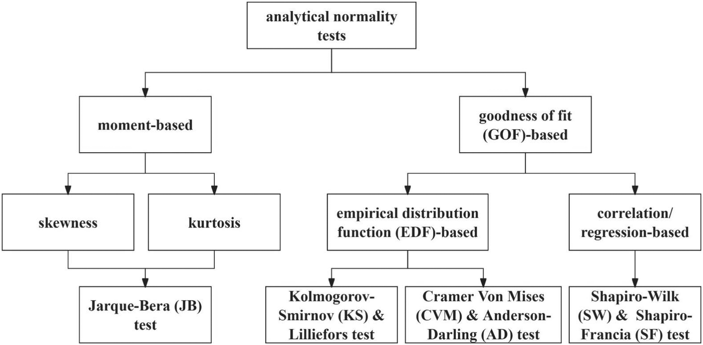
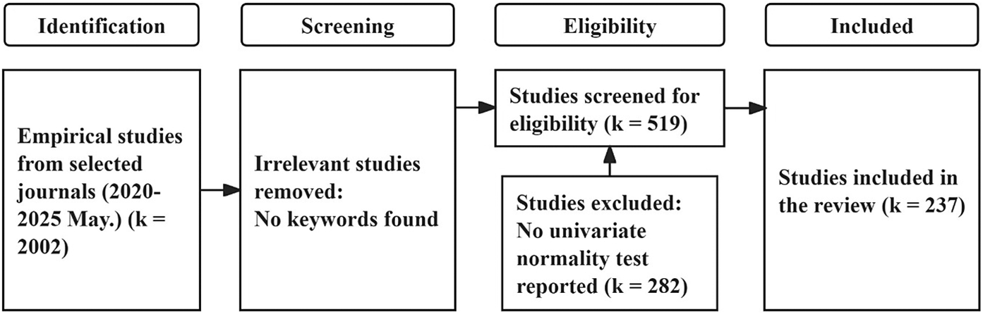
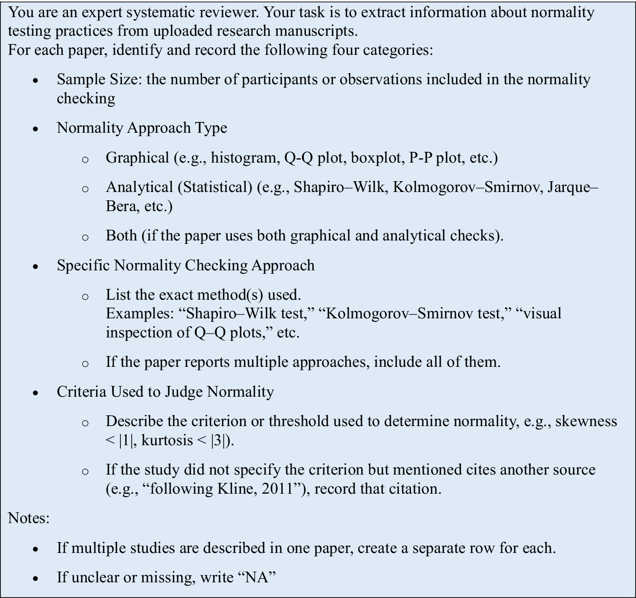

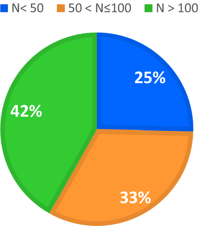
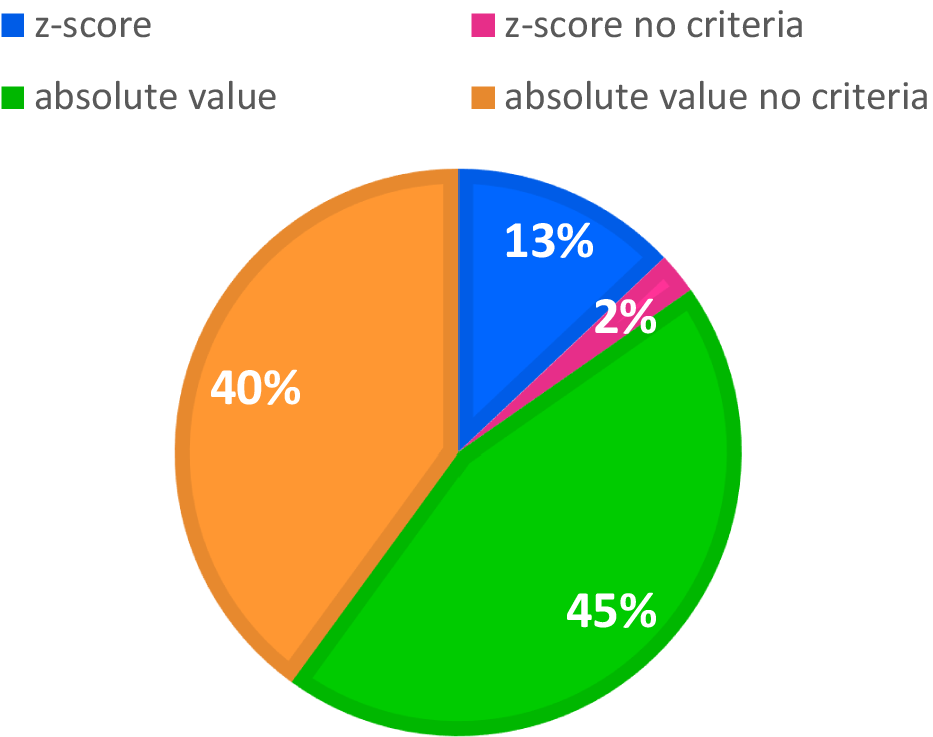


 Open access