


1 Introduction
Beams of high-energy ions can be generated during intense laser–solid interactions, with maximum proton energies exceeding 100 MeV demonstrated to date[
Reference Ziegler, Göthel, Assenbaum, Bernert, Brack, Cowan, Dover, Gaus, Kluge, Kraft, Kroll, Ng, Nishiuchi, Prencipe, Püschel, Rehwald, Reimold, Schlenvoigt, Umlandt, Vescovi, Schramm and Zeil
1
–
Reference Shou, Wu, Pae, Ahn, Kim, Kim, Yoon, Sung, Lee, Gong, Yan, Choi and Nam
3
]. Novel features such as ultra-short bunch duration mean these ion sources have a wide array of potential applications, including fast-ignition inertial confinement fusion (ICF)[
Reference Roth, Cowan, Key, Hatchett, Brown, Fountain, Johnson, Pennington, Snavely, Wilks, Yasuike, Ruhl, Pegoraro, Bulanov, Campbell, Perry and Powell
4
,
Reference Badziak and Domański
5
], proton radiography[
Reference Ostermayr, Kreuzer, Englbrecht, Gebhard, Hartmann, Huebl, Haffa, Hilz, Parodi, Wenz, Donovan, Dyer, Gaul, Gordon, Martinez, McCary, Spinks, Tiwari, Hegelich and Schreiber
6
], radiation damage testing[
Reference Hidding, Karger, Königstein, Pretzler, Manahan, McKenna, Gray, Wilson, Wiggins, Welsh, Beaton, Delinikolas, Jaroszynski, Rosenzweig, Karmakar, Ferlet-Cavrois, Costantino, Muschitiello and Daly
7
,
Reference Ionescu, Gheorghiu, Bobeica, Tataru, Asavei and Leca
8
] and radiobiological research[
Reference Schüller, Heinrich, Fouillade, Subiel, De Marzi, Romano, Peier, Trachsel, Fleta, Kranzer, Caresana, Salvador, Busold, Schönfeld, McEwen, Gomez, Solc, Bailat, Linhart, Jakubek, Pawelke, Borghesi, Kapsch, Knyziak, Boso, Olsovcova, Kottler, Poppinga, Ambrozova, Schmitzer, Rossomme and Vozenin
9
–
Reference Aymar, Becker, Boogert, Borghesi, Bingham, Brenner, Burrows, Ettlinger, Dascalu, Gibson, Greenshaw, Gruber, Gujral, Hardiman, Hughes, Jones, Kirkby, Kurup, Lagrange, Long, Luk, Matheson, McKenna, McLauchlan, Najmudin, Lau, Parsons, Pasternak, Pozimski, Prise, Puchalska, Ratoff, Schettino, Shields, Smith, Thomason, Towe, Weightman, Whyte and Xiao
11
]. Until now, much of the development in laser-driven ion acceleration has been undertaken using high-energy (tens-to-hundreds of joules) lasers and targetry systems that were inherently limited to low (
 $\ll$
1 Hz) repetition rates[
Reference Daido, Nishiuchi and Pirozhkov
12
–
Reference Passoni, Arioli, Cialfi, Dellasega, Fedeli, Formenti, Giovannelli, Maffini, Mirani, Pazzaglia, Tentori, Vavassori, Zavelani-Rossi and Russo
14
]. This limitation has significantly hindered the implementation of statistical and data-driven methodologies, which could be crucial for optimizing and stabilizing ion acceleration mechanisms.
$\ll$
1 Hz) repetition rates[
Reference Daido, Nishiuchi and Pirozhkov
12
–
Reference Passoni, Arioli, Cialfi, Dellasega, Fedeli, Formenti, Giovannelli, Maffini, Mirani, Pazzaglia, Tentori, Vavassori, Zavelani-Rossi and Russo
14
]. This limitation has significantly hindered the implementation of statistical and data-driven methodologies, which could be crucial for optimizing and stabilizing ion acceleration mechanisms.
Supported by advances in high-power laser technology in recent years, a number of petawatt-class high-repetition-rate laser systems have been developed that are capable of greater than or equal to 1 Hz operation[ Reference Danson, Haefner, Bromage, Butcher, Chanteloup, Chowdhury, Galvanauskas, Gizzi, Hein, Hillier, Hopps, Kato, Khazanov, Kodama, Korn, Li, Li, Limpert, Ma, Nam, Neely, Papadopoulos, Penman, Qian, Rocca, Shaykin, Siders, Spindloe, Szatmári, Trines, Zhu, Zhu and Zuegel 15 ]. Such systems have motivated the development of rapidly replaceable targetry such as tape-drive systems[ Reference Dover, Nishiuchi, Sakaki, Kondo, Lowe, Alkhimova, Ditter, Ettlinger, Faenov, Hata, Hicks, Iwata, Kiriyama, Koga, Miyahara, Najmudin, Pikuz, Pirozhkov, Sagisaka, Schramm, Sentoku, Watanabe, Ziegler, Zeil, Kando and Kondo 16 ], liquid crystals[ Reference Poole, Willis, Cochran, Hanna, Andereck and Schumacher 17 ] and cryogenic[ Reference Polz, Robinson, Kalinin, Becker, Fraga, Hellwing, Hornung, Keppler, Kessler, Klöpfel, Liebetrau, Schorcht, Hein, Zepf, Grisenti and Kaluza 18 ] and liquid jets[ Reference Treffert, Glenn, Chou, Crissman, Curry, DePonte, Fiuza, Hartley, Ofori-Okai, Roth, Glenzer and Gauthier 19 ]. As a consequence, it is now possible to produce high-energy laser-driven ion beams at 1 Hz and beyond (see, for example, Ref. [Reference Streeter, Glenn, DiIorio, Treffert, Loughran, Ahmed, Astbury, Borghesi, Bourgeois, Curry, Dann, Dover, Dzelzainis, Ettlinger, Gauthier, Giuffrida, Glenzer, Gray, Green, Hicks, Hyland, Istokskaia, King, Margarone, McCusker, McKenna, Najmudin, Parisuaña, Parsons, Spindloe, Symes, Thomas, Xu and Palmer20]). These efforts have enabled statistical and data-driven experimentation, including machine learning (ML)-based optimization of the ion source[ Reference Loughran, Streeter, Ahmed, Astbury, Balcazar, Borghesi, Bourgeois, Curry, Dann, DiIorio, Dover, Dzelzainis, Ettlinger, Gauthier, Giuffrida, Glenn, Glenzer, Green, Gray, Hicks, Hyland, Istokskaia, King, Margarone, McCusker, McKenna, Najmudin, Parisuaña, Parsons, Spindloe, Symes, Thomas, Treffert, Xu and Palmer 21 , Reference Glenn, Treffert, Ahmed, Astbury, Borghesi, Bourgeois, Curry, Dann, DiIorio, Dover, Dzelzainis, Ettlinger, Gauthier, Giuffrida, Gray, Green, Hicks, Hyland, Istokskaia, King, Loughran, Margarone, McCusker, McKenna, Najmudin, Parisuaña, Parsons, Spindloe, Streeter, Symes, Thomas, Xu, Glenzer and Palmer 22 ] and the generation of training datasets for neural networks to build surrogate models[ Reference Mariscal, Djordjević, Anirudh, Bremer, Campbell, Feister, Folsom, Grace, Hollinger, Jacobs, Kailkhura, Kalantar, Kemp, Kim, Kur, Liu, Ludwig, Morrison, Nedbailo, Ose, Park, Rocca, Scott, Simpson, Song, Spears, Sullivan, Swanson, Thiagarajan, Wang, Williams, Wilks, Wyatt, Van Essen, Zacharias, Zeraouli, Zhang and Ma 23 – Reference McQueen, Wilson, Dolier, Frazer, Ewan, Dzelzainis, Patel, Peat, Torrance, Gray and McKenna 26 ]. These emerging approaches will support the active optimization and stabilization of laser–plasma ion sources, facilitate deeper investigation of the underpinning physics and enhance experimental design – as demonstrated in ICF experiments[ Reference Hatfield, Gaffney, Anderson, Ali, Antonelli, du Pree, Citrin, Fajardo, Knapp, Kettle, Kustowski, MacDonald, Mariscal, Martin, Nagayama, Palmer, Peterson, Rose, Ruby, Shneider, Streeter, Trickey and Williams 27 ]. To fully realize data-driven ion acceleration experiments, it is essential to automate the extraction of key ion beam parameters – such as the energy spectrum, conversion efficiency and maximum energy – at a rate that matches or exceeds the laser repetition rate.
In this paper, we present the algorithm for rapid ion spectrum extraction (ARISE) – a software tool designed for extracting ion energy spectra from a Thomson parabola spectrometer (TPS) at hertz-scale repetition rates, enabling data-driven experimentation with live feedback. ARISE incorporates background subtraction, automatic identification of the zero-deflection reference point (defining the origin of parabolic ion tracks) and automatic determination of the maximum ion energy. At the Scottish Centre for the Application of Plasma-based Accelerators (SCAPA) at the University of Strathclyde, we have developed a laser-driven ion acceleration beamline, which uses a 5 Hz, 350 TW laser for investigation of the physics underpinning laser-driven ion acceleration and for applications such as ultra-high dose rate radiobiology[
Reference Kim, Darafsheh, Schuemann, Dokic, Lundh, Zhao, Ramos-Méndez, Dong and Petersson
28
] and radiation damage studies[
Reference Ishida, Sano, Takahashi, Kojima, Shiraga, Nakatsutsumi, Pikuz, Kado, Arai, Kawaguchi and Okada
29
,
Reference Barberio, Scisciò, Vallières, Cardelli, Chen, Famulari, Gangolf, Revet, Schiavi, Senzacqua and Antici
30
]. We demonstrate the performance of the ARISE using the SCAPA laser–ion beamline operating at 0.2 Hz, a rate constrained solely by data transfer speeds and the readout time of the diagnostic camera. Integrated into a feedback loop, ARISE performed real-time ion spectral analysis to autonomously guide and optimize the maximum energy of laser-accelerated protons. Furthermore, we show that ARISE can process ion spectra at rates exceeding 20 Hz when applied to representative archival experimental data. We validate its accuracy in both spectrum extraction and automatic detection of the maximum proton energy (
 ${E}_{\mathrm{p},\max }$
), highlighting its suitability for high-throughput ion diagnosis in data-driven laser–plasma experiments.
${E}_{\mathrm{p},\max }$
), highlighting its suitability for high-throughput ion diagnosis in data-driven laser–plasma experiments.
2 Ion spectrometer design and data capture
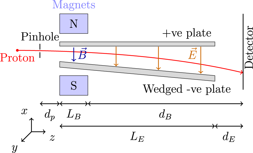
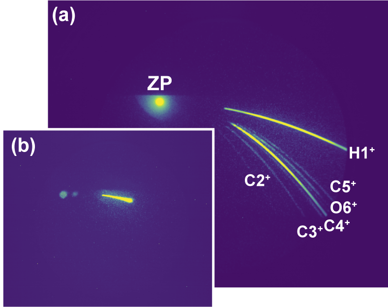
A TPS separates ions based on their kinetic energy and charge-to-mass ratio, producing characteristic parabolic traces[ Reference Thomson 31 ]. In this work, we employed the TPS design reported by Carroll et al. [ Reference Carroll, Brummitt, Neely, Lindau, Lundh, Wahlström and McKenna 32 ], the operating principle of which is illustrated in Figure 1. The spectrometer featured a 500 μm diameter pinhole to limit angular acceptance. Ions were deflected by a 0.6 T magnetic dipole pair and a pair of wedged electric plates, across which a total potential difference of 5 kV was applied. The ions were then detected by a microchannel plate (MCP) coupled to a phosphor screen (Hamamatsu F2226-14PF143). The end of the electric plates was positioned 75 mm upstream of the MCP. The resulting parabolic ion traces were recorded using a 16-bit scientific complementary metal–oxide–semiconductor (sCMOS) camera (Andor Neo) and example measurements are shown in Figure 2(a). The geometry and dimensions of the magnetic and electric field regions matched those described by Carroll et al. [ Reference Carroll, Brummitt, Neely, Lindau, Lundh, Wahlström and McKenna 32 ].
Schematic view of the Thomson parabola spectrometer in the
 $x$
–
$x$
–
 $z$
plane. The electric and magnetic fields are both oriented along the
$z$
plane. The electric and magnetic fields are both oriented along the
 $x$
-axis, resulting in ion dispersion along the
$x$
-axis, resulting in ion dispersion along the
 $x$
- and
$x$
- and
 $y$
-axes due to their respective influences.
$y$
-axes due to their respective influences.
(a) Representative MCP phosphor screen image showing the reference zero point (ZP), corresponding to undeflected neutral atoms and X-rays, and a set of ion tracks (H, hydrogen; C, carbon; O, oxygen; with given charge states). (b) An example MCP phosphor screen image showing the filtered ion signal through 200 μm thick Mylar, for the energy calibration.
2.1 Charged particle trajectories in a Thomson parabola spectrometer
Charged particles entering a TPS are deflected by electric and magnetic fields, with their motion governed by the non-relativistic Lorentz force:
 $$\begin{align}\vec{F}=q\left(\vec{E}+\vec{v}\times \vec{B}\right),\end{align}$$
where
 $q$
is the particle charge,
$q$
is the particle charge,
 $\vec{v}$
is its velocity and
$\vec{v}$
is its velocity and
 $\vec{E}$
and
$\vec{E}$
and
 $\vec{B}$
are the electric and magnetic fields, respectively.
$\vec{B}$
are the electric and magnetic fields, respectively.
In the small-angle approximation, the transverse displacements resulting from the electric and magnetic fields – accounting for a drift region between the field termination and the detector – are approximately given by the following:
 $$\begin{align}x\sim \frac{q\mid \vec{E}\mid {L}_{\mathrm{E}}}{mv_z^2}\left(\frac{L_{\mathrm{E}}}{2}+{d}_{\mathrm{E}}\right), \end{align}$$
 $$\begin{align}y\sim \frac{q\mid \vec{B}\mid {L}_{\mathrm{B}}}{mv_z}\left(\frac{L_{\mathrm{B}}}{2}+{d}_{\mathrm{B}}\right),\end{align}$$
where
 ${L}_{\mathrm{E}}$
and
${L}_{\mathrm{E}}$
and
 ${L}_{\mathrm{B}}$
are the effective lengths of the electric and magnetic field regions, respectively,
${L}_{\mathrm{B}}$
are the effective lengths of the electric and magnetic field regions, respectively,
 ${d}_{\mathrm{E}}$
and
${d}_{\mathrm{E}}$
and
 ${d}_{\mathrm{B}}$
are the distances from the end of each field region to the detector plane, respectively,
${d}_{\mathrm{B}}$
are the distances from the end of each field region to the detector plane, respectively,
 $m$
is the mass of the particle and
$m$
is the mass of the particle and
 ${v}_z$
is the longitudinal component of the velocity.
${v}_z$
is the longitudinal component of the velocity.
These expressions describe the characteristic parabolic traces observed in a TPS under the assumption of uniform fields. However, in the present setup employing a wedged electrode design, the fields are inherently non-uniform, necessitating a more general approach to modelling ion trajectories.
Assuming a constant particle mass
 $m$
, and defining the velocity and position vectors as
$m$
, and defining the velocity and position vectors as
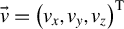 $\vec{v}={\left({v}_x,{v}_y,{v}_z\right)}^{\mathrm{T}}$
and
$\vec{v}={\left({v}_x,{v}_y,{v}_z\right)}^{\mathrm{T}}$
and
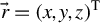 $\vec{r}={\left(x,y,z\right)}^{\mathrm{T}}$
, Newton’s second law provides the time evolution of the velocity:
$\vec{r}={\left(x,y,z\right)}^{\mathrm{T}}$
, Newton’s second law provides the time evolution of the velocity:
 $$\begin{align}\frac{\mathrm{d}\vec{v}}{\mathrm{d}t}=\frac{q}{m}\left(\vec{E}+\vec{v}\times \vec{B}\right).\end{align}$$
To determine the full trajectory, we also evolve the following position:
 $$\begin{align}\frac{\mathrm{d}\vec{r}}{\mathrm{d}t}=\vec{v}.\end{align}$$
Rather than integrating these equations in time and checking when the particle reaches a fixed longitudinal position (e.g.,
 $z={z}_{\mathrm{det}}$
), it is often advantageous to reparameterize the system using
$z={z}_{\mathrm{det}}$
), it is often advantageous to reparameterize the system using
 $z$
as the independent variable. This approach simplifies numerical integration in systems where
$z$
as the independent variable. This approach simplifies numerical integration in systems where
 $z$
increases monotonically.
$z$
increases monotonically.
Applying the chain rule:
 $$\begin{align}\frac{\mathrm{d}}{\mathrm{d}t}=\frac{\mathrm{d}z}{\mathrm{d}t}\cdot \frac{\mathrm{d}}{\mathrm{d}z}={v}_z\frac{\mathrm{d}}{\mathrm{d}z},\end{align}$$
the equations of motion can be rewritten as follows:
 $$\begin{align}\frac{\mathrm{d}\vec{r}}{\mathrm{d}z}&=\frac{\vec{v}}{v_z}, \end{align}$$
 $$\begin{align}\frac{\mathrm{d}\vec{v}}{\mathrm{d}z}&=\frac{q}{mv_z}\left(\vec{E}+\vec{v}\times \vec{B}\right).\end{align}$$
Equations (7) and (8) form a coupled system of six first-order ordinary differential equations (ODEs) with respect to
 $z$
: three governing the components of velocity and three for the components of position.
$z$
: three governing the components of velocity and three for the components of position.
The equations of motion are then solved numerically using the solve_ivp solver from the scipy.integrate module in Python[
Reference Virtanen, Gommers, Oliphant, Haberland, Reddy, Cournapeau, Burovski, Peterson, Weckesser, Bright, van der Walt, Brett, Wilson, Millman, Mayorov, Nelson, Jones, Kern, Larson, Carey, Polat, Feng, Moore, VanderPlas, Laxalde, Perktold, Cimrman, Henriksen, Quintero, Harris, Archibald, Ribeiro, Pedregosa and van Mulbregt
33
], over a predefined range of particle energies and charge states for the electric and magnetic fields determined by the TPS design geometry, potential difference and magnetic field strength. The resulting transverse displacements
 $\left(x,y\right)$
at the detector produce the characteristic parabolic traces of a TPS.
$\left(x,y\right)$
at the detector produce the characteristic parabolic traces of a TPS.
2.2 Data capture
To enable data acquisition and preparation for ARISE at the necessary repetition rate, we employ custom data capture and management software. This system facilitates real-time acquisition and handling of all laser data, metadata and diagnostics associated with a given experiment. It also supports automated control of the laser system and target delivery, and can execute grid scans or implement Bayesian optimization algorithms[ Reference Dolier, King, Wilson, Gray and McKenna 34 , Reference Shahriari, Swersky, Wang, Adams and de Freitas 35 ]. When combined with ARISE, this analysis framework enables fully automated, real-time optimization of key proton beam parameters on the SCAPA beamline, as elaborated in Section 4.1.
3 ARISE structure and functionality
This section outlines the core functionality provided by ARISE for the automated extraction of ion spectra from unprocessed images of the TPS parabolas. Key features include automatic background subtraction, zero-point (ZP) detection, spectral extraction and identification of the maximum ion energy. The implementation of these components for spectral analysis is illustrated schematically in Figure 3.
Flow diagram illustrating the main components of the ARISE processing pipeline. The workflow begins with user-defined parameters specified in the configuration file, followed by data acquisition from the CCD (MCP image). The image then undergoes a series of processing steps, including zero-point detection, cropping, rotation and background subtraction. The resulting image is subsequently passed to the spectral extraction module and the automated detection of
 ${E}_{\mathrm{p},\max }$
.
${E}_{\mathrm{p},\max }$
.
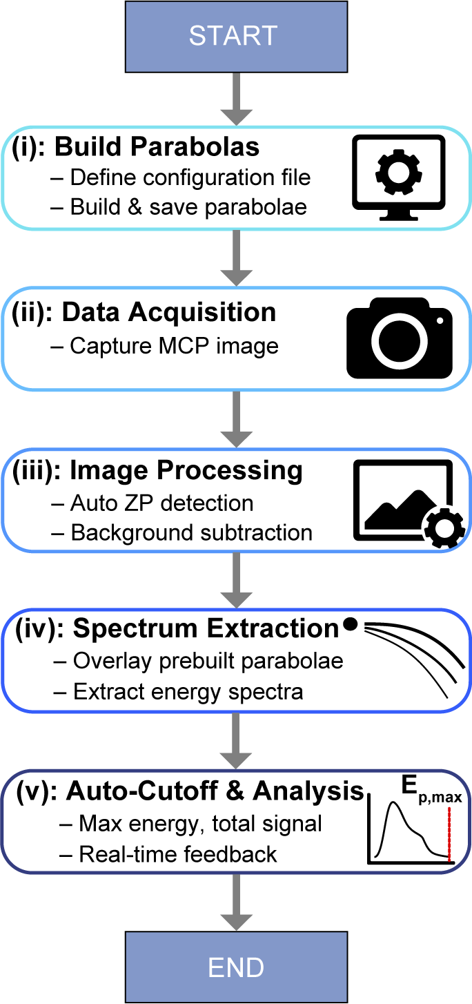
The various steps are as follows.
(i) The initial stage of ARISE analysis requires the user to define fixed design parameters of the TPS within a configuration file. These parameters include the spectrometer geometry, the potential difference across the electrode plates, the magnetic field strength, the spatial calibration of the camera and the range of ion energies to be extracted.
Based on this configuration, ARISE constructs the predicted ion parabolic tracks for a given TPS design, ion species and specified energy range. For each predefined energy increment, the ion deflection coordinates are computed using a numerical solver for the coupled system of ODEs described in Section 2, which models the ion trajectory through the regions
 ${L}_{\mathrm{E}}$
,
${L}_{\mathrm{E}}$
,
 ${L}_{\mathrm{B}}$
,
${L}_{\mathrm{B}}$
,
 ${d}_{\mathrm{E}}$
and
${d}_{\mathrm{E}}$
and
 ${d}_{\mathrm{B}}$
. The resulting deflections are first calculated in real space and subsequently converted into pixel coordinates using the spatial calibration. These coordinates define sampling paths along the parabolic tracks, enabling the extraction of ion signal intensity corresponding to discrete energy bins.
${d}_{\mathrm{B}}$
. The resulting deflections are first calculated in real space and subsequently converted into pixel coordinates using the spatial calibration. These coordinates define sampling paths along the parabolic tracks, enabling the extraction of ion signal intensity corresponding to discrete energy bins.
One of the inherent limitations of a TPS is the potential overlap of neighbouring species’ tracks as they converge at higher ion energies. To address this, the ARISE issues an alert when track overlap is detected, enabling the user to take corrective action to minimize such occurrences – for example, by increasing dispersion through a higher field strength or by positioning the detector further from the fields. The algorithm includes a dedicated class that can be activated by setting a corresponding flag in the configuration file to True, which enables the detection of ion species overlap. A second flag can similarly be set to True to construct truncated parabolas; that is, the parabolas are terminated at the point of overlap, beyond which the ion species can no longer be identified with certainty. This truncation feature can be enabled via the configuration file, and the newly generated parabolas can be stored for subsequent use.
Due to the nonlinear relationship between particle energy and deflection, the spatial separation between adjacent energy bins decreases at higher energies. To mitigate the resampling of identical pixels across adjacent bins, ARISE removes duplicate pixel coordinates and assigns each pixel a representative energy value, calculated as the average of its contributing energies.
While ion trajectories (parabolas) can be recalculated for each newly acquired signal, doing so can be computationally intensive depending on the energy resolution, thereby limiting the repetition rate of analysis. However, as the ion deflection paths depend only on fixed geometrical and field parameters – which are assumed to remain constant between shots – ARISE addresses this limitation by storing precomputed parabolas for each TPS configuration. This significantly reduces processing speed by enabling their reuse in subsequent analyses.
(ii) Once the ion trajectories have been either calculated or loaded from a prebuilt parabola file, unprocessed MCP images can be acquired for analysis.
(iii) The acquired image of the MCP phosphor screen is then processed to extract the ion spectra. ARISE includes an automatic detection routine to identify the point of zero deflection – hereafter referred to as the ZP – which typically consists of undeflected neutral particles and X-rays. The ZP represents the origin of the processed image and is the convergence point of all ion parabolas. An example of the ZP position relative to the ion tracks is shown in Figure 2(a).
The ZP detection feature initially employs image erosion techniques (see, for example, Ref. [Reference Haralick, Sternberg and Zhuang36]) to eliminate saturated pixels and then identifies the coordinates of maximum intensity. Optionally, a region of interest (ROI) can be specified around the expected ZP location, reducing computation time and minimizing interference from other bright regions in the image. The approximate ZP coordinates are defined in the configuration file, from which ARISE constructs the ROI for targeted erosion and peak detection.
Once the ZP has been identified, the next stage involves subtracting the background from the image. Initially, a median filter (see, for example, Refs. [Reference Virtanen, Gommers, Oliphant, Haberland, Reddy, Cournapeau, Burovski, Peterson, Weckesser, Bright, van der Walt, Brett, Wilson, Millman, Mayorov, Nelson, Jones, Kern, Larson, Carey, Polat, Feng, Moore, VanderPlas, Laxalde, Perktold, Cimrman, Henriksen, Quintero, Harris, Archibald, Ribeiro, Pedregosa and van Mulbregt33,Reference Pitas and Venetsanopoulos37]) may be applied across the entire image. This filter computes, for each pixel, the median value within its surrounding region – defined by a user-specified kernel size – in order to suppress impulse noise such as isolated high-signal pixels resulting from detector noise or high-energy X-rays, as well as to mitigate the effects of dead or abnormally responsive pixels, while preserving sharp edges. The filtering process has been implemented in a multi-threaded manner to enhance computational efficiency by dividing the image into smaller segments – whose number is specified in the configuration file – processing them in parallel, and subsequently reconstructing the full image.
Empirical analysis of hundreds of measurements indicated that assuming a radially symmetric background centred on the ZP provides the best agreement with observed background signal characteristics. To ensure accurate background estimation, regions beyond the phosphor screen and areas surrounding the ion tracks are masked out to avoid contamination of the background model. A saturation check is then performed within the ion track region, during which the user is notified if saturation occurs and to what extent. Specifically, if the proportion of saturated pixels exceeds a user-defined threshold (for example,
 $>$
1%), an alert is issued, prompting the user to adjust the MCP amplification accordingly. Then, for each radial distance from the ZP, the average signal value is calculated and adjusted using a standard deviation multiplier, configurable by the user, to determine the threshold for background subtraction. In our dataset, we found that subtracting values exceeding the average by four standard deviations yielded the most reliable results in terms of isolating the ion signal.
$>$
1%), an alert is issued, prompting the user to adjust the MCP amplification accordingly. Then, for each radial distance from the ZP, the average signal value is calculated and adjusted using a standard deviation multiplier, configurable by the user, to determine the threshold for background subtraction. In our dataset, we found that subtracting values exceeding the average by four standard deviations yielded the most reliable results in terms of isolating the ion signal.
Alternative methods for background subtraction – including Otsu’s method[ Reference Bangare, Dubal, Bangare and Patil 38 ], sampling from tracks parallel to the ion trajectories and background ROI sampling – were also investigated. However, these approaches were found to perform less effectively, both in terms of background removal accuracy and computational efficiency.
(iv) Following background subtraction, the ion spectrum is extracted along the previously defined ion tracks. For each track, two additional bounding parabolas are constructed to enclose the full spatial width of the ion signal, determined by the dimensions of the TPS pinhole. The sampled track width,
 $\delta$
, is calculated using the TPS geometry as follows:
$\delta$
, is calculated using the TPS geometry as follows:
 $$\begin{align}\delta =d+\left(s+d\right)\kern0.1em \frac{L_{\mathrm{E}}+{d}_{\mathrm{E}}+{d}_{\mathrm{p}}}{L},\end{align}$$
where
 $d$
is the pinhole diameter,
$d$
is the pinhole diameter,
 $s$
is the effective source size,
$s$
is the effective source size,
 ${d}_{\mathrm{p}}$
is the distance from the pinhole to the start of the electric plates and
${d}_{\mathrm{p}}$
is the distance from the pinhole to the start of the electric plates and
 $L$
is the source-to-pinhole distance[
Reference Rajeev, Rishad, Trivikram, Narayanan and Krishnamurthy
39
]. At each energy step, a lineout is extracted perpendicular to the trajectory defined between the bounding parabolas. The sum of pixel values along this lineout provides a measure of signal intensity as a function of ion energy, corresponding to the relative number of detected ions.
$L$
is the source-to-pinhole distance[
Reference Rajeev, Rishad, Trivikram, Narayanan and Krishnamurthy
39
]. At each energy step, a lineout is extracted perpendicular to the trajectory defined between the bounding parabolas. The sum of pixel values along this lineout provides a measure of signal intensity as a function of ion energy, corresponding to the relative number of detected ions.
While it is possible to convert these pixel counts into absolute ion numbers using established calibration methods[ Reference Prasad, Doria, Ter-Avetisyan, Fostera, Quinn, Romagnani, Brenner, Green, Gallegos, Streeter, Carroll, Tresca, Dover, Palmer, Schreiber, Neely, Najmudin, McKenna, Zepf and Borghesi 40 – Reference Harres, Schollmeier, Brambrink, Audebert, Blažević, Flippo, Gautier, Geißel, Hegelich, Nürnberg, Schreiber, Wahl and Roth 42 ], an absolute calibration has not yet been implemented in the current version of ARISE. Work is underway to perform such a calibration, following methodologies similar to those described by Harres et al. [ Reference Harres, Schollmeier, Brambrink, Audebert, Blažević, Flippo, Gautier, Geißel, Hegelich, Nürnberg, Schreiber, Wahl and Roth 42 ].
(v) Finally, from the extracted spectrum, key physical quantities are derived in real time, including the maximum ion energy and total signal intensity, corresponding to the total ion flux. The approach can easily be extended to extract other quantities, such as the spectral temperature of the distribution. These outputs are used both to inform experimental decision-making and to support data-driven optimization routines aimed at enhancing the quality and performance of the ion source.
4 Code performance and validation
In this section, we evaluate the performance of key features within the ARISE framework, through both verification tests and application to real-time experimental data.
4.1 Verification of model accuracy and energy measurements
A central requirement of ARISE is the robust and reliable automatic detection of the maximum proton energy for a given proton spectrum. This capability is critical for supporting optimization and stability studies of laser-driven ion sources. Prior to implementing and assessing automated detection routines, we first validated the accuracy of the ion energies predicted by the ARISE deflection model.
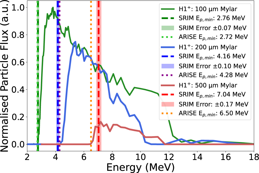
To validate both the accuracy of the ion deflection model within ARISE and the energy resolution of the TPS, selected regions of the MCP were covered with Mylar foils of known thickness, designed to stop protons of specific energies as calculated using SRIM software[
Reference Ziegler, Ziegler and Biersack
43
]. Calibration was performed using multiple filter configurations to provide several reference points. This involved applying Mylar sheets with thicknesses of 100, 200 or 500 μm across the entire MCP, with an example MCP phosphor screen image shown in Figure 2(b) (corresponding to the 200 μm case). Each filter thickness imposes a minimum detectable proton energy,
 ${E}_{\mathrm{p},\min }$
, beyond which protons can reach the detector without being stopped in the Mylar. The values of
${E}_{\mathrm{p},\min }$
, beyond which protons can reach the detector without being stopped in the Mylar. The values of
 ${E}_{\mathrm{p},\min }$
, calculated using SRIM simulations[
Reference Stoller, Toloczko, Was, Certain, Dwaraknath and Garner
44
], were 2.76
${E}_{\mathrm{p},\min }$
, calculated using SRIM simulations[
Reference Stoller, Toloczko, Was, Certain, Dwaraknath and Garner
44
], were 2.76
 $\pm$
0.07, 4.16
$\pm$
0.07, 4.16
 $\pm$
0.10 and 7.04
$\pm$
0.10 and 7.04
 $\pm$
0.17 MeV for the respective filters. These values were used as benchmarks to validate the energy calibration and accuracy of the ARISE deflection model.
$\pm$
0.17 MeV for the respective filters. These values were used as benchmarks to validate the energy calibration and accuracy of the ARISE deflection model.
As shown in Figure 4, there is good agreement between the minimum proton energies
 ${E}_{\mathrm{p},\min }$
predicted by ARISE and those expected based on filter thickness. Specifically, ARISE returned values of 2.72, 4.28 and 6.50 MeV, compared to the expected values of 2.76
${E}_{\mathrm{p},\min }$
predicted by ARISE and those expected based on filter thickness. Specifically, ARISE returned values of 2.72, 4.28 and 6.50 MeV, compared to the expected values of 2.76
 $\pm$
0.07, 4.16
$\pm$
0.07, 4.16
 $\pm$
0.10 and 7.04
$\pm$
0.10 and 7.04
 $\pm$
0.17 MeV, respectively. For the thickest filter, there is evidence of increased ion scattering, manifested as a broadening of the apparent minimum energy. In addition, the nonlinear spacing of energy bins at higher energies, inherent to the TPS geometry, leads to reduced accuracy in the predicted
$\pm$
0.17 MeV, respectively. For the thickest filter, there is evidence of increased ion scattering, manifested as a broadening of the apparent minimum energy. In addition, the nonlinear spacing of energy bins at higher energies, inherent to the TPS geometry, leads to reduced accuracy in the predicted
 ${E}_{\mathrm{p},\min }$
in this regime. Nevertheless, across all cases, the predicted values remain in good agreement with those calculated using the SRIM model, confirming the reliability of the ODE-based deflection solver within ARISE.
${E}_{\mathrm{p},\min }$
in this regime. Nevertheless, across all cases, the predicted values remain in good agreement with those calculated using the SRIM model, confirming the reliability of the ODE-based deflection solver within ARISE.
Measured proton spectra from energy calibration shots. Dashed red, blue and green lines denote the expected minimum transmission energies,
 ${E}_{\mathrm{p},\min }$
, based on SRIM simulations. Dash-dotted orange, purple and light green lines indicate the corresponding
${E}_{\mathrm{p},\min }$
, based on SRIM simulations. Dash-dotted orange, purple and light green lines indicate the corresponding
 ${E}_{\mathrm{p},\min }$
values calculated using ARISE. Shaded regions represent uncertainties in the SRIM-derived energy thresholds, defined by the extent of lateral straggling.
${E}_{\mathrm{p},\min }$
values calculated using ARISE. Shaded regions represent uncertainties in the SRIM-derived energy thresholds, defined by the extent of lateral straggling.
Following this validation of the modelled energy values, we evaluated several approaches for automatic detection of the maximum proton energy,
 ${E}_{\mathrm{p},\max }$
. A dataset of 15 randomly selected spectra was extracted from experimentally acquired measurements. For each spectrum, a ground truth value of
${E}_{\mathrm{p},\max }$
. A dataset of 15 randomly selected spectra was extracted from experimentally acquired measurements. For each spectrum, a ground truth value of
 ${E}_{\mathrm{p},\max }$
was established through blind manual assessment by four independent researchers, each unaware of the others’ selections and the results of any automated method. The ground truth value was defined as the mean of these manual assessments, and the associated standard deviation was used to quantify uncertainty. An automated method is considered well calibrated if its output lies within this confidence interval.
${E}_{\mathrm{p},\max }$
was established through blind manual assessment by four independent researchers, each unaware of the others’ selections and the results of any automated method. The ground truth value was defined as the mean of these manual assessments, and the associated standard deviation was used to quantify uncertainty. An automated method is considered well calibrated if its output lies within this confidence interval.
To assess performance, we present the two best-performing
 ${E}_{\mathrm{p},\max }$
detection methods and summarize their results against the ground truth data.
${E}_{\mathrm{p},\max }$
detection methods and summarize their results against the ground truth data.
The first of these methods – the less effective of the two – identifies
 ${E}_{\mathrm{p},\max }$
by evaluating the local gradient of the ion spectrum and selecting the energy at which the gradient consistently falls below a user-defined threshold. Although conceptually straightforward, this approach is highly sensitive to the chosen threshold parameter, which is somewhat arbitrary and set in the configuration file. As a result, the method is prone to false positives or premature termination, particularly in the presence of noise or weak signal gradients near the high-energy cut-off.
${E}_{\mathrm{p},\max }$
by evaluating the local gradient of the ion spectrum and selecting the energy at which the gradient consistently falls below a user-defined threshold. Although conceptually straightforward, this approach is highly sensitive to the chosen threshold parameter, which is somewhat arbitrary and set in the configuration file. As a result, the method is prone to false positives or premature termination, particularly in the presence of noise or weak signal gradients near the high-energy cut-off.
The second method evaluated is based on a least squares regression technique previously applied to time-of-flight ion spectrometers[ Reference Russell, Istokskaia, Giuffrida, Levy, Huynh, Cimrman, Srmž and Margarone 45 ]. For a given spectrum, a sliding least squares regression is implemented for successive windows of neighbouring data points along the spectrum. For each window, the gradient and intercept of the best-fit line are computed according to Equations (10) and (11):
 $$\begin{align}m&=\frac{N{\sum}_{i=1}^N{x}_i{y}_i-{\sum}_{i=1}^N{x}_i{\sum}_{i=1}^N{y}_i}{N{\sum}_{i=1}^N{x}_i^2-{\left({\sum}_{i=1}^N{x}_i\right)}^2},\end{align}$$
 $$\begin{align}c&=\frac{\sum_{i=1}^N{x}_i^2{\sum}_{i=1}^N{y}_i-{\sum}_{i=1}^N{x}_i{\sum}_{i=1}^N{x}_i{y}_i}{N{\sum}_{i=1}^N{x}_i^2-{\left({\sum}_{i=1}^N{x}_i\right)}^2}.\end{align}$$
Here,
 $x$
and
$x$
and
 $y$
denote the particle energy and particle flux, respectively, and
$y$
denote the particle energy and particle flux, respectively, and
 $N=2r+1$
is the number of data points included in each local fit, with
$N=2r+1$
is the number of data points included in each local fit, with
 $r$
being a user-defined parameter specified in the configuration file. The gradient and intercept of each local fit are denoted by
$r$
being a user-defined parameter specified in the configuration file. The gradient and intercept of each local fit are denoted by
 $m$
and
$m$
and
 $c$
, respectively. The maximum proton energy,
$c$
, respectively. The maximum proton energy,
 ${E}_{\mathrm{p},\max }$
, is identified as the point where the final calculated local slope crosses the x-intercept, corresponding to zero flux.
${E}_{\mathrm{p},\max }$
, is identified as the point where the final calculated local slope crosses the x-intercept, corresponding to zero flux.
Empirical testing showed that this method performs most reliably for small window sizes, specifically when
 $r\le 2$
and
$r\le 2$
and
 $N\le 5$
. This approach offers a key advantage over the fixed-threshold method, as the transition to the background level is determined intrinsically from the spectral shape, rather than through a user-defined parameter.
$N\le 5$
. This approach offers a key advantage over the fixed-threshold method, as the transition to the background level is determined intrinsically from the spectral shape, rather than through a user-defined parameter.
A comparative analysis of the two methods is presented in Figure 5 and Table 1.
(a) Example spectrum comparing automatic
 ${E}_{\mathrm{p},\max }$
detection using two methods, least squares regression (blue dashed line) and the threshold method (orange dashed line), compared against the ground truth (red solid line). (b) Comparison of
${E}_{\mathrm{p},\max }$
detection using two methods, least squares regression (blue dashed line) and the threshold method (orange dashed line), compared against the ground truth (red solid line). (b) Comparison of
 ${E}_{\mathrm{p},\max }$
values across 15 spectra, showing results from least squares regression (blue circles) and the threshold method (red circles) relative to the ground truth. The black dashed line indicates the ideal
${E}_{\mathrm{p},\max }$
values across 15 spectra, showing results from least squares regression (blue circles) and the threshold method (red circles) relative to the ground truth. The black dashed line indicates the ideal
 $y=x$
agreement. Error bars represent standard deviations from the ground truth. A representative case where the threshold method fails is also highlighted (red dashed line).
$y=x$
agreement. Error bars represent standard deviations from the ground truth. A representative case where the threshold method fails is also highlighted (red dashed line).
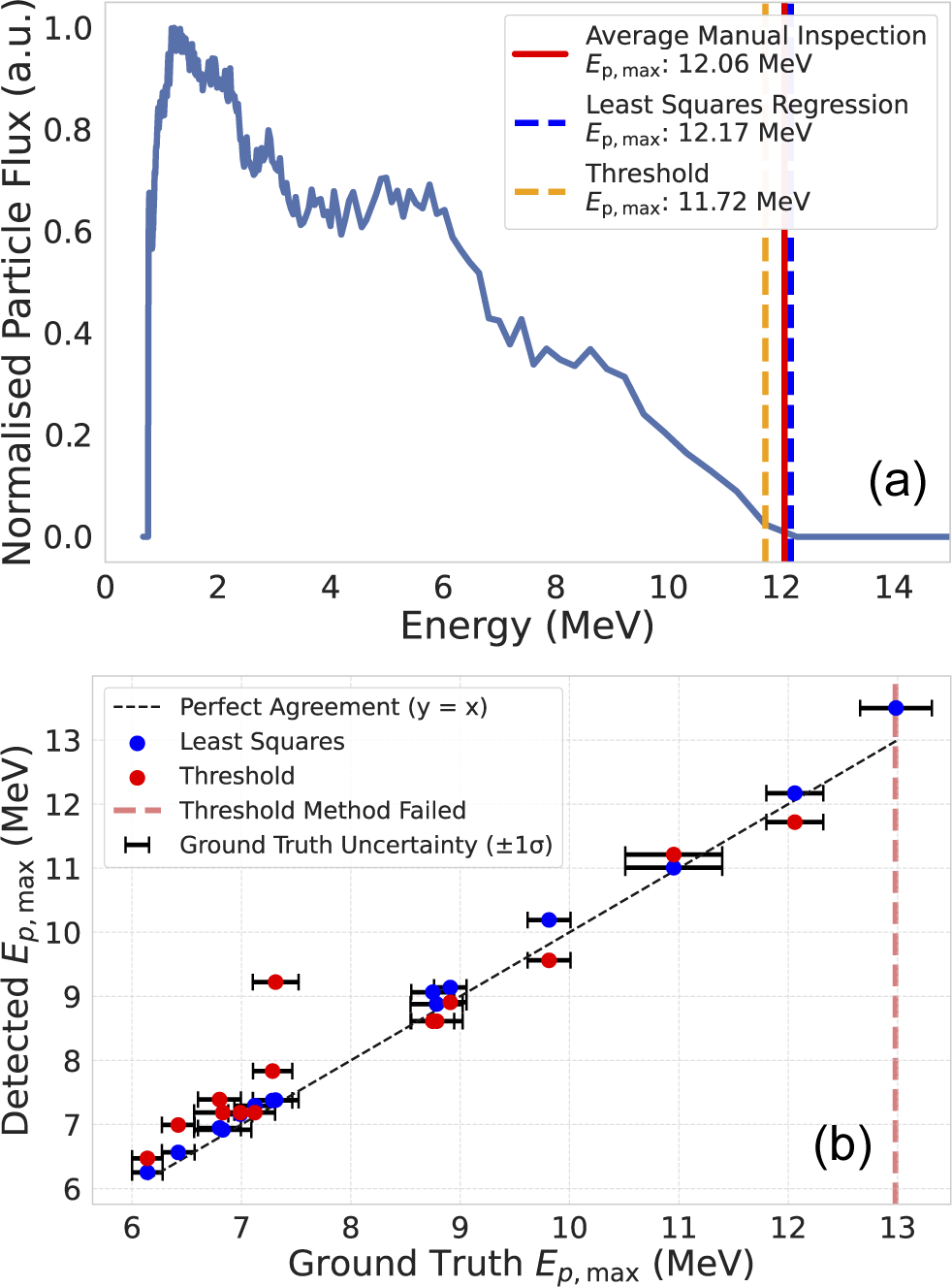
Figure 5(a) shows a representative ion spectrum with the ground truth and automatically detected
 ${E}_{\mathrm{p},\max }$
values annotated. In this case, the gradient threshold method significantly underperforms relative to the least squares regression, with respect to the ground truth. To explore this further, Figure 5(b) presents a comparison of both methods against ground truth values across all 15 analysed spectra. The black dashed line indicates the case of ideal agreement between the ground truth and detected
${E}_{\mathrm{p},\max }$
values annotated. In this case, the gradient threshold method significantly underperforms relative to the least squares regression, with respect to the ground truth. To explore this further, Figure 5(b) presents a comparison of both methods against ground truth values across all 15 analysed spectra. The black dashed line indicates the case of ideal agreement between the ground truth and detected
 ${E}_{\mathrm{p},\max }$
values, with the error bars representing the standard deviation in the ground truth value. While neither method is perfectly calibrated, the least squares approach consistently outperforms the threshold method.
${E}_{\mathrm{p},\max }$
values, with the error bars representing the standard deviation in the ground truth value. While neither method is perfectly calibrated, the least squares approach consistently outperforms the threshold method.
Table 1 quantitatively compares the two methods using multiple performance metrics, including the mean absolute error (MAE), root mean square error (RMSE) and mean absolute percentage error (MAPE). Across all metrics, the least squares method outperforms the threshold approach by more than a factor of two. The ‘Within
 $1{\sigma}_{\mathrm{human}}$
’ row further highlights that approximately two-thirds of least squares results fall within one standard deviation of the human-assessed ground truth, compared to just over one-third for the threshold method.
$1{\sigma}_{\mathrm{human}}$
’ row further highlights that approximately two-thirds of least squares results fall within one standard deviation of the human-assessed ground truth, compared to just over one-third for the threshold method.
Performance comparison of
 ${E}_{\mathrm{p},\max }$
detection methods. The least squares method significantly outperforms the threshold method, achieving a root mean square error (RMSE) of 0.22 MeV compared to 0.61 MeV. To contextualize these results, we introduce a normalized error metric that compares the automated detection error to the uncertainty in the human-assessed ground truth. Specifically, RMSE values are normalized by the mean standard deviation of the ground truth estimates. Using this metric, the performance of the least squares method is found to be comparable to that of human assessment.
${E}_{\mathrm{p},\max }$
detection methods. The least squares method significantly outperforms the threshold method, achieving a root mean square error (RMSE) of 0.22 MeV compared to 0.61 MeV. To contextualize these results, we introduce a normalized error metric that compares the automated detection error to the uncertainty in the human-assessed ground truth. Specifically, RMSE values are normalized by the mean standard deviation of the ground truth estimates. Using this metric, the performance of the least squares method is found to be comparable to that of human assessment.
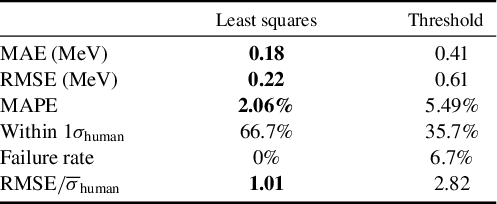
To assess performance in relation to the uncertainty inherent in the ground truth itself, we introduce a normalized metric: the RMSE of each method divided by the mean standard deviation of the human inspection values,
 ${\overline{\sigma}}_{\mathrm{human}}$
. This dimensionless metric reflects model performance relative to typical human disagreement. A ratio less than or equal to 1 indicates parity with human reliability; values of more than 1 suggest inferior accuracy. The least squares method yields a value of 1.01, suggesting performance on par with human annotation, while the threshold method returns 2.82, indicating significantly poorer accuracy. In addition, the gradient threshold method exhibits a higher failure rate and a tendency for ‘brittleness’[
Reference Spencer
46
], with catastrophic failures observed in certain cases (e.g., no value returned, indicated by the red dashed line in Figure 5(b)). This behaviour makes it unsuitable for use in unsupervised data-driven optimization processes.
${\overline{\sigma}}_{\mathrm{human}}$
. This dimensionless metric reflects model performance relative to typical human disagreement. A ratio less than or equal to 1 indicates parity with human reliability; values of more than 1 suggest inferior accuracy. The least squares method yields a value of 1.01, suggesting performance on par with human annotation, while the threshold method returns 2.82, indicating significantly poorer accuracy. In addition, the gradient threshold method exhibits a higher failure rate and a tendency for ‘brittleness’[
Reference Spencer
46
], with catastrophic failures observed in certain cases (e.g., no value returned, indicated by the red dashed line in Figure 5(b)). This behaviour makes it unsuitable for use in unsupervised data-driven optimization processes.
Testing the ARISE repetition rate – a key aspect of ARISE development is not only the ability to automatically extract ion spectra, but also do so at repetition rates exceeding 1 Hz. This capability is essential for real-time optimization of the ion source, as well as for collecting statistically significant datasets and large-scale training sets for ML models.
To validate the maximum effective repetition rate of ARISE, 200 MCP phosphor images from an existing dataset acquired at the SCAPA facility were analysed using ARISE. The analysis was initialized using a prebuilt proton parabola covering the energy range 0.25–20 MeV. The time taken to complete each major processing step in ARISE – background subtraction, multi-threaded median filtering, image handling (including cropping and rotation), automatic ZP detection and automatic
 ${E}_{\mathrm{p},\max }$
extraction – was recorded to identify potential bottlenecks affecting throughput. The computer system used is equipped with an AMD EPYC 9454 processor operating at 2.75 GHz.
${E}_{\mathrm{p},\max }$
extraction – was recorded to identify potential bottlenecks affecting throughput. The computer system used is equipped with an AMD EPYC 9454 processor operating at 2.75 GHz.
When all processing steps are enabled, the average time per image is 292
 $\pm$
6 ms, corresponding to a repetition rate of 3.42
$\pm$
6 ms, corresponding to a repetition rate of 3.42
 $\pm$
0.07 Hz. The dominant time contributions arise from image processing – particularly background subtraction and median filtering – which together account for approximately 83
$\pm$
0.07 Hz. The dominant time contributions arise from image processing – particularly background subtraction and median filtering – which together account for approximately 83
 $\%$
of the total analysis time. Median filtering was originally implemented to mitigate noise and suppress hot pixels due to hard X-ray hits in earlier datasets. However, more recent data obtained with improved detector shielding indicate that this step is unnecessary. As shown in Figure 6(a), when median filtering is omitted, the repetition rate increases significantly to 20
$\%$
of the total analysis time. Median filtering was originally implemented to mitigate noise and suppress hot pixels due to hard X-ray hits in earlier datasets. However, more recent data obtained with improved detector shielding indicate that this step is unnecessary. As shown in Figure 6(a), when median filtering is omitted, the repetition rate increases significantly to 20
 $\pm$
2 Hz, with a mean processing time of 49
$\pm$
2 Hz, with a mean processing time of 49
 $\pm$
6 ms – substantially exceeding the repetition rate of many high-power laser systems and leaving significant allowance for data transfer and the execution of optimization routines[
Reference Feister, Cassou, Dann, Döpp, Gauron, Gonsalves, Joglekar, Marshall, Neveu, Schlenvoigt, Streeter and Palmer
47
].
$\pm$
6 ms – substantially exceeding the repetition rate of many high-power laser systems and leaving significant allowance for data transfer and the execution of optimization routines[
Reference Feister, Cassou, Dann, Döpp, Gauron, Gonsalves, Joglekar, Marshall, Neveu, Schlenvoigt, Streeter and Palmer
47
].
(a) Bar chart showing the average processing time for key stages of ARISE, with and without median filtering, across 200 data points. The most time-consuming steps are median filtering (when applied) and background subtraction. Without filtering, the pipeline achieves an average repetition rate of 20.40 Hz; applying median filtering reduces this rate significantly to 3.42 Hz. (b) Average repetition rate as a function of the number of ion species, based on 200 shots. Error bars represent one standard deviation in processing time.
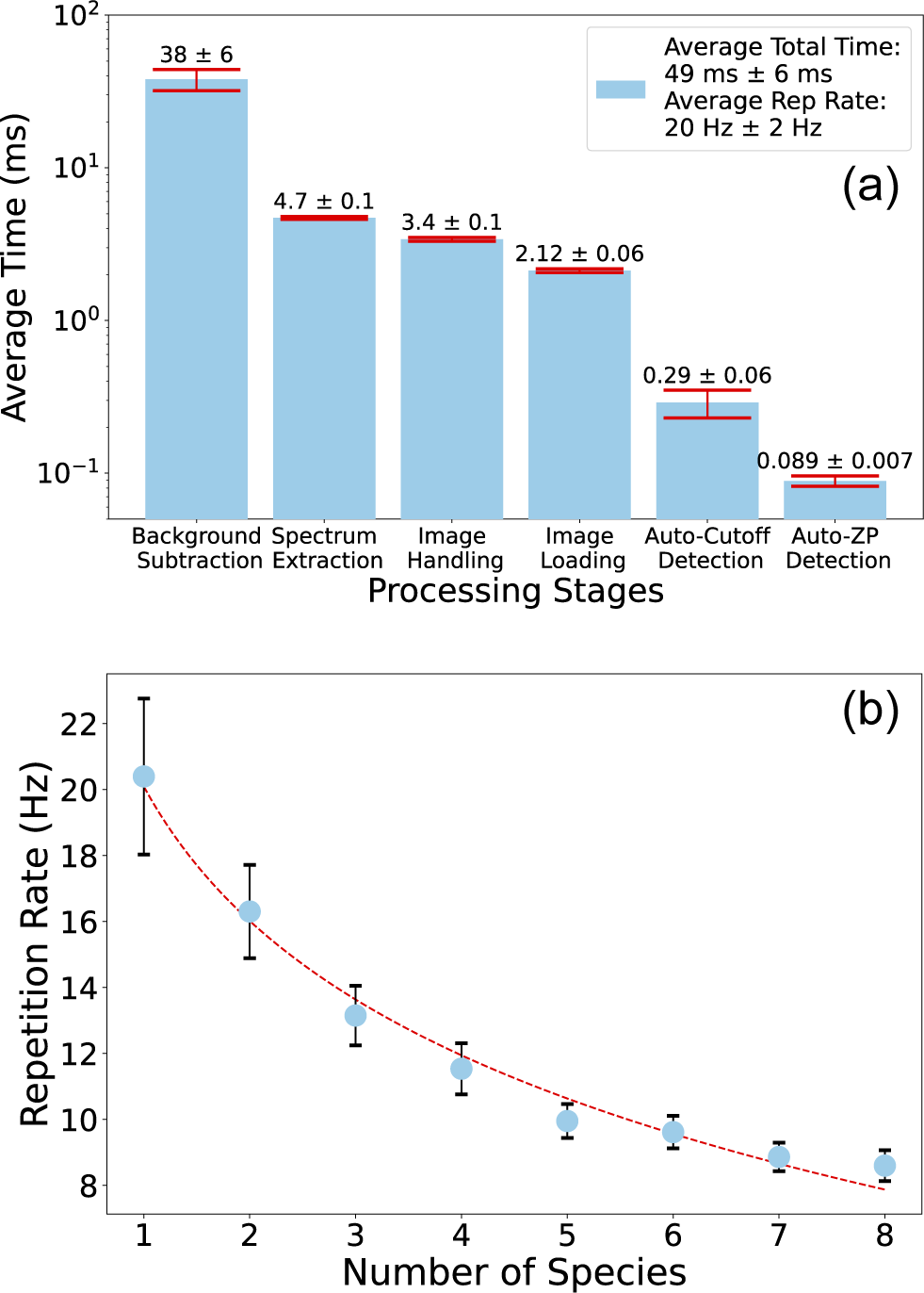
To evaluate the impact of analysing multiple ion species (e.g., various charge states of carbon and oxygen), the average repetition rate was measured as a function of the number of species processed using the same dataset. The results are shown in Figure 6(b). Each species was analysed over the energy range of 0.25–20 MeV (total energy, not per nucleon), using 0.1 MeV energy bins. As expected, the repetition rate decreases with increasing species number, falling from its maximum for a single species to 8.60
 $\pm$
0.47 Hz when eight species are included. Since image processing is only performed once per image, the overall analysis time scales sub-linearly with the number of species, and the observed reduction in repetition rate represents only a factor of approximately 2.3.
$\pm$
0.47 Hz when eight species are included. Since image processing is only performed once per image, the overall analysis time scales sub-linearly with the number of species, and the observed reduction in repetition rate represents only a factor of approximately 2.3.
4.2 Real-time experimental demonstration
A real-time experimental validation of ARISE was conducted using the 5 Hz, 350 TW SCAPA laser. Laser pulses of 5.39
 $\pm$
0.08 J energy and 29.6
$\pm$
0.08 J energy and 29.6
 $\pm$
0.4 fs duration were focused to a 1.57
$\pm$
0.4 fs duration were focused to a 1.57
 $\pm$
0.04 μm (full width at half maximum, FWHM) spot onto 10 μm thick steel tape and, in a separate run, onto 13 μm thick Kapton tape targets. During this demonstration the effective repetition rate was limited to 0.2 Hz due to constraints in data transfer speed to the server where data was stored for analysis by ARISE and the readout rate of the diagnostic camera.
$\pm$
0.04 μm (full width at half maximum, FWHM) spot onto 10 μm thick steel tape and, in a separate run, onto 13 μm thick Kapton tape targets. During this demonstration the effective repetition rate was limited to 0.2 Hz due to constraints in data transfer speed to the server where data was stored for analysis by ARISE and the readout rate of the diagnostic camera.
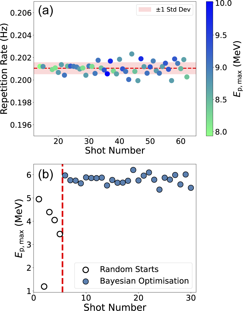
In a preliminary demonstration of real-time capability, repeated proton beam measurements were performed without deliberate modification of experimental parameters. Under these stable conditions, ARISE consistently measured
 ${E}_{\mathrm{p},\max }$
, as shown in Figure 7(a), highlighting its ability to actively monitor proton beam properties during periods of stable operation.
${E}_{\mathrm{p},\max }$
, as shown in Figure 7(a), highlighting its ability to actively monitor proton beam properties during periods of stable operation.
(a) Example of automatic
 ${E}_{\mathrm{p},\max }$
extraction (colour axis) across more than 60 shots at a repetition rate of 0.2 Hz. The shaded region corresponds to one standard deviation. (b) Results from an experiment where ARISE-derived
${E}_{\mathrm{p},\max }$
extraction (colour axis) across more than 60 shots at a repetition rate of 0.2 Hz. The shaded region corresponds to one standard deviation. (b) Results from an experiment where ARISE-derived
 ${E}_{\mathrm{p},\max }$
values were used as the objective function in an open-source Bayesian optimization feedback loop, in which laser energy and pulse duration were varied by the optimizer. Unfilled symbols represent initial random sampling, while filled symbols correspond to values selected using the Gaussian process regression model. The dashed red line separates the random sampling phase from the model-driven optimization phase.
${E}_{\mathrm{p},\max }$
values were used as the objective function in an open-source Bayesian optimization feedback loop, in which laser energy and pulse duration were varied by the optimizer. Unfilled symbols represent initial random sampling, while filled symbols correspond to values selected using the Gaussian process regression model. The dashed red line separates the random sampling phase from the model-driven optimization phase.

To further demonstrate the performance of ARISE in undertaking real-time ion spectra analysis and facilitating data-driven optimization, the automatically determined
 ${E}_{\mathrm{p},\max }$
values were used as the objective function in a Bayesian optimization feedback loop[
Reference Pedregosa, Varoquaux, Gramfort, Michel, Thirion, Grisel, Blondel, Prettenhofer, Weiss, Dubourg, Vanderplas, Passos, Cournapeau, Brucher, Perrot and Duchesnay
48
], implemented within our experimental control software[
Reference Dolier, King, Wilson, Gray and McKenna
34
] and interfaced directly with SCAPA control systems.
${E}_{\mathrm{p},\max }$
values were used as the objective function in a Bayesian optimization feedback loop[
Reference Pedregosa, Varoquaux, Gramfort, Michel, Thirion, Grisel, Blondel, Prettenhofer, Weiss, Dubourg, Vanderplas, Passos, Cournapeau, Brucher, Perrot and Duchesnay
48
], implemented within our experimental control software[
Reference Dolier, King, Wilson, Gray and McKenna
34
] and interfaced directly with SCAPA control systems.
The results of the optimization run are presented in Figure 7(b). To initialize the Bayesian optimization process, five shots were taken with randomized laser energy and pulse duration values, within the ranges of 0.28–2.7 J (restricted to mitigate risk of damaging the focusing optic) and 25–135 fs, respectively. The pulse duration was varied using the group delay dispersion (GDD) of a Dazzler system[
Reference Verluise, Laude, Cheng, Spielmann and Tournois
49
]. The GDD value corresponding to the shortest pulse duration was 23,000 fs
 ${}^2$
. During optimization, this value was allowed to vary within the range of 21,800–24,000 fs
${}^2$
. During optimization, this value was allowed to vary within the range of 21,800–24,000 fs
 ${}^2$
. Owing to the relationship between GDD and pulse duration, this range enables variation of the pulse duration around its minimum value, and the explored pulse duration range corresponds to a GDD variation of approximately 1000 fs
${}^2$
. Owing to the relationship between GDD and pulse duration, this range enables variation of the pulse duration around its minimum value, and the explored pulse duration range corresponds to a GDD variation of approximately 1000 fs
 ${}^2$
. For each shot, ARISE determined the maximum proton energy,
${}^2$
. For each shot, ARISE determined the maximum proton energy,
 ${E}_{\mathrm{p},\max }$
, which was then used to train an initial Gaussian process regression (GPR) model[
Reference Rasmussen and Williams
50
], thereby initiating the Bayesian optimization routine targeting maximization of
${E}_{\mathrm{p},\max }$
, which was then used to train an initial Gaussian process regression (GPR) model[
Reference Rasmussen and Williams
50
], thereby initiating the Bayesian optimization routine targeting maximization of
 ${E}_{\mathrm{p},\max }$
.
${E}_{\mathrm{p},\max }$
.
In this simple two-parameter optimization example, Figure 7(b) shows that ARISE successfully returns the variation in
 ${E}_{\mathrm{p},\max }$
from the random parameter sampling (unfilled symbols) to construct the GPR model that enables the Bayesian optimization routine to rapidly reach a plateau for maximum laser energy (filled symbols), as expected. Variation in pulse duration variation across the set GDD range was found to have negligible impact on
${E}_{\mathrm{p},\max }$
from the random parameter sampling (unfilled symbols) to construct the GPR model that enables the Bayesian optimization routine to rapidly reach a plateau for maximum laser energy (filled symbols), as expected. Variation in pulse duration variation across the set GDD range was found to have negligible impact on
 ${E}_{\mathrm{p},\max }$
, consistent with Zimmer et al.
[
Reference Zimmer, Scheuren, Ebert, Schaumann, Schmitz, Hornung, Bagnoud, Rödel and Roth
51
]. This proof-of-principle demonstration of real-time optimization using only two parameters highlights the capability of ARISE for integration into more complex multi-parameter optimization frameworks[
Reference Loughran, Streeter, Ahmed, Astbury, Balcazar, Borghesi, Bourgeois, Curry, Dann, DiIorio, Dover, Dzelzainis, Ettlinger, Gauthier, Giuffrida, Glenn, Glenzer, Green, Gray, Hicks, Hyland, Istokskaia, King, Margarone, McCusker, McKenna, Najmudin, Parisuaña, Parsons, Spindloe, Symes, Thomas, Treffert, Xu and Palmer
21
,
Reference Dolier, King, Wilson, Gray and McKenna
34
] and its potential to enable fully automated tuning of laser-driven proton sources in future experimental campaigns.
${E}_{\mathrm{p},\max }$
, consistent with Zimmer et al.
[
Reference Zimmer, Scheuren, Ebert, Schaumann, Schmitz, Hornung, Bagnoud, Rödel and Roth
51
]. This proof-of-principle demonstration of real-time optimization using only two parameters highlights the capability of ARISE for integration into more complex multi-parameter optimization frameworks[
Reference Loughran, Streeter, Ahmed, Astbury, Balcazar, Borghesi, Bourgeois, Curry, Dann, DiIorio, Dover, Dzelzainis, Ettlinger, Gauthier, Giuffrida, Glenn, Glenzer, Green, Gray, Hicks, Hyland, Istokskaia, King, Margarone, McCusker, McKenna, Najmudin, Parisuaña, Parsons, Spindloe, Symes, Thomas, Treffert, Xu and Palmer
21
,
Reference Dolier, King, Wilson, Gray and McKenna
34
] and its potential to enable fully automated tuning of laser-driven proton sources in future experimental campaigns.
5 Conclusions
In summary, we have developed and demonstrated ARISE – an algorithm capable of real-time extraction of laser-driven ion spectra at repetition rates exceeding 20 Hz. Its key features include automatic detection of the zero-deflection reference point, background subtraction and identification of the maximum ion energy. In addition, it has been deployed to support real-time optimization of the maximum proton energy via a Bayesian optimization algorithm. ARISE autonomously extracted
 ${E}_{\mathrm{p},\max }$
in real time and this value was used by the Bayesian optimization algorithm to determine the optimal drive laser parameters. During this experiment, the maximum achievable repetition rate was 0.2 Hz, constrained solely by data transfer speed and the diagnostic charge-coupled device (CCD) readout time. Performance testing has demonstrated that ARISE can be applied at multi-hertz repetition rates.
${E}_{\mathrm{p},\max }$
in real time and this value was used by the Bayesian optimization algorithm to determine the optimal drive laser parameters. During this experiment, the maximum achievable repetition rate was 0.2 Hz, constrained solely by data transfer speed and the diagnostic charge-coupled device (CCD) readout time. Performance testing has demonstrated that ARISE can be applied at multi-hertz repetition rates.
The development of ARISE represents a significant step towards automated, high-repetition-rate, data-driven optimization of laser-driven ion sources. Beyond experimental control, it enables the rapid generation of training datasets for neural network-based synthetic diagnostics[ Reference McQueen, Wilson, Dolier, Frazer, Ewan, Dzelzainis, Patel, Peat, Torrance, Gray and McKenna 26 ] during live experiments, using the well-established TPS. This capability will facilitate the discovery of new strategies to stabilize and control ion beam properties, advancing progress towards real-world applications[ Reference Hatfield, Gaffney, Anderson, Ali, Antonelli, du Pree, Citrin, Fajardo, Knapp, Kettle, Kustowski, MacDonald, Mariscal, Martin, Nagayama, Palmer, Peterson, Rose, Ruby, Shneider, Streeter, Trickey and Williams 27 ]. Furthermore, ARISE is easily adaptable to the automated analysis of other charged particle spectrometers, including electron spectrometers[ Reference Roy and Tremblay 52 ] and wide-angle ion spectrometers[ Reference Jung, Hörlein, Gautier, Letzring, Kiefer, Allinger, Albright, Shah, Palaniyappan, Yin, Fernández, Habs and Hegelich 53 ], promoting broader adoption of data-driven approaches in laser–plasma diagnostics.
Acknowledgements
This work was financially supported by EPSRC (grant numbers EP/R006202/1, EP/V049232/1, EP/P020607/1, EP/X525017/1 and EP/Z535692/1) and STFC (grant numbers ST/V001612/1 and ST/X005895/1). Studentship funding from Dstl is gratefully acknowledged. Data associated with research published in this paper can be accessed at: https://doi.org/10.15129/24453482-da0e-424b-822e-6d0a42ce911d.


 Open access