

Introduction
Pine Island Glacier (PIG) ice shelf, the floating tongue of the fastest ice stream in West Antarctica, has experienced recent acceleration and thinning (Reference RignotRignot, 2008; Reference Scott, Gudmundsson, Smith, Bingham, Pritchard and VaughanScott and others, 2009; Reference Wingham, Wallis and ShepherdWingham and others, 2009), and its grounding line has the potential for sustained long-term retreat (Reference JenkinsJenkins and others, 2010). The recent changes are mainly due to rapid melting by relatively warm ocean waters accessing the grounding zone and base of the ice shelf (Reference Jacobs, Hellmer and JenkinsJacobs and others, 1996, Reference Jacobs, Jenkins, Giulivi and Dutrieux2011; Reference Jenkins, Vaughan, Jacobs, Hellmer and KeysJenkins and others, 1997; Reference Hellmer, Jacobs, Jenkins, Jacobs and WeissHellmer and others, 1998; Reference Shepherd, Wingham and RignotShepherd and others, 2004; Reference Payne, Holland, Shepherd, Rutt, Jenkins and JoughinPayne and others, 2007; Reference Bindschadler, Vaughan and VornbergerBindschadler and others, 2011). Reference Bindschadler, Vaughan and VornbergerBindschadler and others (2011) inferred that buoyant water beneath the PIG ice shelf is at least partly accommodated by flow in channels carved into the bottom of the ice shelf. That finding would have important implications for planning in situ measurements of sub-ice-shelf circulation and for quantitative modeling of such circulation.
Here we focus on the nature of sub-ice-shelf channels near the ice-shelf terminus and their influence on ocean properties and circulation and sea-ice variability in the adjacent Pine Island Bay (PIB). Our findings extend modeling and other observational studies that have suggested or revealed inverted channels beneath ice shelves (Reference Payne, Holland, Shepherd, Rutt, Jenkins and JoughinPayne and others, 2007; Reference Rignot and SteffenRignot and Steffen, 2008; Reference Bindschadler, Vaughan and VornbergerBindschadler and others, 2011; personal communication from D. Vaughan, 2011).
Data and Methodology
We use 441 Moderate Resolution Imaging Spectroradiometer (MODIS), Landsat and Advanced Very High Resolution Radiometer (AVHRR) images from 1986 to 2011 of the PIG ice shelf and PIB region in the southeast Amundsen Sea (see Appendix for data sources). We examined each image for the presence of full sea-ice cover, small polynyas (open water bounded by ice, as in Fig. 1), coastal leads or full open water.
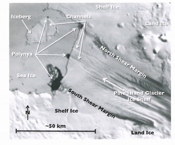
The Pine Island Glacier ice shelf and adjacent ice-covered Pine Island Bay in a MODIS satellite image acquired 16 January 2004. The ~40km wide, rapidly moving ice extends ~70km from the grounded glacier, its sides defined by darker shear margins as it pushes past more slowly moving floating shelf ice and grounded land ice to the north and south. Flowlines evolve toward the calving front, where both shear margins and central lineations terminate near small regions of open water (polynyas). Smaller polynyas appear near the ends of similar features on an iceberg that calved in 2001.
Airplane overflights in November 2009 provided surface height from an Airborne Topographic Mapper (ATM) and thickness from a Multichannel Coherent Radar Depth Sounder Level 2 (MCoRDS) (Reference AllenAllen, 2009; Reference KrabillKrabill, 2009; Reference Koenig, Martin, Studinger and SonntagKoenig and others, 2010). Ice thickness measurements have an along-track resolution of ~35m and a vertical resolution of ~20m (https://www.cresis.ku.edu/sites/default/files/data-files/Antarctica/2009_chile/Readme.pdf). We calculated the ice base below sea level (draft when floating) from the surface elevation and ice thickness data by averaging the 15 nearest elevation points (i.e. 500m along-track) to each thickness point and then subtracting elevation from thickness (Fig. 2).
PIG ice shelf terminus from a MODIS image acquired 30 January 2009 when open water (black) was present in PIB and the shear margins were well defined. The upper-panel PP′ and QQ′ lines show the positions of overflights (Reference Koenig, Martin, Studinger and SonntagKoenig and others, 2010), colored as ice draft (thickness minus elevation). The lower-panel PP′ (gray) and QQ′ (black) lines profile measured elevation and derived draft relative to the sea surface. Vertical dashed lines define the ice shelf within its shear margins. N and W are the narrow and wide central inverted basal channels on QQ′, flanked by a more deeply cut channel across the southern shear margin and a broader channel with a data gap at the northern margin due to heavy crevassing. The locations of CTD (+) and XBT (×) casts are shown near the ice front, as in Figure 3, along with sea surface temperature (SST) and salinity, offset here for clarity, and shown across the full ice width above Figure 3b.

In January 2009 a research cruise mapped ocean properties near the PIG ice shelf terminus. Ocean water column profiling for temperature, salinity and currents was conducted with a conductivity–temperature–depth (CTD) instrument using a SeaBird SBE 911+ system with a Lowered Acoustic Doppler Current Profiler (LADCP), and for temperature by Sippican T-7 eXpendable Bathy-Thermograph (XBT) casts. Sea surface temperature (SST) and sea surface salinity data were acquired underway with an SBE 45 flow-through thermosalinograph (TSG) at ~6m depth (Fig. 3).
Ocean temperature, salinity, and current velocity ~500m seaward of the PIG ice shelf calving front. (a) CTD temperatures in color and salinity contours. (b) XBT temperature in color and ice-shelf draft ~10km upstream along the QQ′ line (Fig. 2) plotted in gray, with N and W marking the narrow and wide channels. Temperature and salinity near the sea surface along the ship track is shown above. (c) CTD depth-averaged anomaly in color, salinity anomaly contoured, and ice-shelf draft. (d) XBT depth-averaged anomaly, current velocities at –30, –15, –7, –3.5, 0 and +3.5 cm s–1 (positive eastward) and ice-shelf draft. Gray shading is sea-floor, no data, and invalid data. Even profile spacing here approximates actual cast positions in Figure 2. The CTD and XBT transects were occupied on 18 and 28 January 2009.

Sea surface skin temperatures representing the top few micrometers (Reference DonlonDonlon and others, 2002) were derived from Landsat thermal infrared (TIR) bands using standard ENVI software routines and a bias correction (Fig. 4; see also Reference Bindschadler, Vaughan and VornbergerBindschadler and others, 2011, fig. 14). Surface skin values a few degrees below the freezing point (–1.86˚C) may reflect grease ice formed by offshore winds at –12˚C on 16 November 2008 when the image was acquired (http://efdl_5cims.nyu.edu/timeseries/NYU_AWS_PIGo_timeseries.html), but are unrealistic for the ocean surface mixed layer. The lowest TIR temperatures were thus adjusted to the freezing point, resulting in values within 0.2˚C of the 10m surface layer average on 26 CTD casts over 9 days in January 2009 near and including CTD 16 (Fig. 2 and 3).
Landsat Enhanced Thematic Mapper Plus (ETM+) thermal infrared image of PIB and the PIG ice shelf, acquired 16 November 2008, prior to the January 2009 ship-based fieldwork. The bay appears to be mostly open water at this time, with the highest surface temperatures appearing directly seaward of the southern shear margin and weaker signatures near the central and northern ice-shelf front. Outflows from beneath the ice shelf have become entrained and mix in a large cyclonic gyre in PIB.

Results
Surface lineations
The PIG ice shelf consists of a fast-flowing central region, flanked by nearly stagnant shelf ice to its north and south. A 2004 MODIS image (Fig. 1) shows linear and curved surface features on its fast- and slow-moving parts. Grounded obstacles under moving ice often generate surface flowline features that are parallel and extend linearly downstream of the basal bumps (Reference Gudmundsson, Raymond and BindschadlerGudmundsson and others, 1998). The lineations may begin near the grounding line, but evolve seaward after the glacier has decoupled from its bed. Curvilinear features may be caused by lateral stress or by sub-ice-shelf hydrologic processes such as focused areas of enhanced melt in the moving ice. Mostly linear but nonparallel surface lineations are also visible on the grounded iceberg in Figure 1, which calved in 2001. Tracking the iceberg positions back to the calving event in satellite imagery shows its surface lineations once connected with those on the ice shelf. Elevation data reveal that many of the primary visual lineations correspond to surface ridges and depressions in the floating ice shelf. The two central features (N and W in Fig. 2) have topographic variability of 10–20 m.
Subsurface channels
Ice thickness data indicate subsurface inverted channels below the surface topographic lows (Fig. 2), confirming the supposition of Reference Bindschadler, Vaughan and VornbergerBindschadler and others (2011) that the surface troughs are likely underlain by basal channels due to hydrostatic equilibrium. Broad but not detailed agreement is evident between ice elevations and drafts along overflight transect PP′ and downstream transect QQ′ (Fig. 2). Apparent channel misalignments between the two sections could result from the curvilinear nature of some corresponding surface and basal features, along with channel widening or coalescence downstream. Most of the thinnest ice corresponds to the north and south shear margins, the dark (low-brightness) and wide bands in Figures 1 and 2. These features are generated by large velocity gradients where fast-flowing ice from PIG moves past the slower parts of the ice shelf. The northern margin is wider on the outer ice shelf, perhaps due to topographic highs in the sea-floor, while the southern margin displays large height and draft differences between PP′ and QQ′. Floating slow-moving shelf ice at the southern end of PP′ has probably allowed the primary, Coriolis-deflected outflow plume (Reference Payne, Holland, Shepherd, Rutt, Jenkins and JoughinPayne and others, 2007; Reference Holland, Jenkins and HollandHolland and others, 2008) to extend well beyond the southern shear margin. Evidence for this detour can also be seen in the sinuous surface lineations (Fig. 1) and the low elevations and drafts along PP′ south of the southern shear margin (Fig. 2). The outflow must return to its main channel before reaching QQ′, the right-hand side of which is over grounded ice to the south of that margin.
According to Reference Joughin, Smith and HollandJoughin and others (2010), the ice shelf was moving at ~4kma–1, a travel time of ~2.5 years between PP′ and QQ′. Between the shear margins (vertical dashed line in lower panel of Fig. 2), both transects have a mean height of 58 m and a thickness of 437 m, roughly consistent with along-flow profiles of the ice shelf (Reference Bindschadler, Vaughan and VornbergerBindschadler and others, 2011), and a draft-to-freeboard ratio of 85%, both in and out of the channels. This suggests little if any basal melting on the outer ice shelf, within the ±20m accuracy of the thickness measurements. Nonetheless, the channels do evolve between the transects: along QQ′, a narrow channel reduces the ice draft to ~200 m, and a 3.6 km wide channel to its south appears to be linked to three narrower channels along PP′ (Fig. 2) and to the ocean measurements.
Oceanographic data at the ice front
Temperature and salinity data from CTD and XBT profiles along the PIG ice shelf terminus show a halocline between warm, salty, weakly stratified Circumpolar Deep Water (CDW) below ~600m and seasonally modified surface waters above ~400m that also contain mixtures of CDW and ice-shelf meltwater (Fig. 3a and b; also Reference Jacobs, Jenkins, Giulivi and DutrieuxJacobs and others, 2011). When the CDW comes in contact with deep ice near the grounding line, it gains meltwater and buoyancy, flowing along the bottom of the ice shelf where the basal morphology exerts a strong control on the melt parameters (Reference Little, Gnanadesikan and OppenheimerLittle and others, 2009).
The CTD and XBT transects are ~10 days apart and average ~500m distant from the ice front. To calculate depth-averaged anomalies, we averaged all column profiles to determine a mean depth profile and then subtracted this from each individual profile (Fig. 3c and d). Three prominent warm features appear in the upper 350 m. The largest, near the southern shear margin (CTD16/XBT66), would be expected from the general cyclonic circulation in PIB and under the ice shelf (Reference Hellmer, Jacobs, Jenkins, Jacobs and WeissHellmer and others, 1998; Reference Payne, Holland, Shepherd, Rutt, Jenkins and JoughinPayne and others, 2007) in combination with a vertical circulation of inflow at depth and outflow at shallower levels (Reference Jacobs, Hellmer and JenkinsJacobs and others, 1996; Reference Holland, Jenkins and HollandHolland and others, 2008; Reference Olbers and HellmerOlbers and Hellmer, 2010). Another large subsurface positive anomaly occurs slightly south of the wide central channel (CTD19/ XBT55–57; W in Figs 2 and 3b). A SST and salinity anomaly also appears above the deepest basal incision (CTD21/ XBT54; N in Figs 2 and 3b, line plots above N in Fig. 3b). Westward (negative, out of the PIG ice shelf cavity) current velocities in Figure 3d were strongest off the southern shear margin and present near the central anomaly region. The current measurements are generally consistent with temperatures and geostrophic calculations (Reference Jacobs, Jenkins, Giulivi and DutrieuxJacobs and others, 2011), indicating weak inflow of CDW on the northern half of the section and stronger, slightly cooled outflow to the south (Fig. 3c and d). A second CTD transect ~10 km seaward of the ice-shelf front (not shown) displayed a weaker, more dispersed central subsurface anomaly, shifted southward with the cyclonic circulation in PIB.
Polynyas at the ice front
Aerial and satellite imagery of the PIG ice shelf began in 1947 (Reference RignotRignot, 2002) and 1963 (Reference Kim, Jezek and LiuKim and others, 2007) respectively, and one to three small polynyas have frequently appeared at the calving front (as in Fig. 1) in the historical record (Reference BindschadlerBindschadler, 2002; Reference Scambos, Raup and BohlanderScambos and others, 2009; Reference Bindschadler, Vaughan and VornbergerBindschadler and others, 2011). Summarizing the temporal characteristics of these features from 1972/73 through 2007/08 in ~125 mostly Landsat observations, Reference Bindschadler, Vaughan and VornbergerBindschadler and others (2011) noted their fixed locations, persistence during summer after 1998/99, and an altered pattern in the last year possibly related to a rifting and calving event. Polynya positions near the sides and middle of the fast-flowing part of the PIG ice shelf roughly coincided with the sites of subsurface melt-laden outflows modeled by Reference Payne, Holland, Shepherd, Rutt, Jenkins and JoughinPayne and others (2007), leading to inferences of sufficient residual heat and buoyancy that plumes could rise to the surface and melt sea ice.
Antarctic polynyas are common in winter where offshore winds drive newly formed sea ice away from the coast, often coupled with adjacent promontories that block the alongshore drift of sea ice (Reference Massom, Harris, Michael and PotterMassom and others, 1998; Reference Martin, Steele, Turekian and ThorpeMartin, 2002). This process can cause warmer sea water to upwell from below, and warmer seasonal conditions can also produce spring/summer polynyas. In PIB the sea-ice field is often ‘fast’, i.e. frozen to the ice front, even during summer, and the prevailing large-scale southeasterlies are unlikely to generate such small polynyas (Fig. 5b and circles in Fig. 5a). Also, offshore winds typically generate coastal leads and larger-scale open water features when sea ice is detached from the coastline (Fig. 5c and the ovals in Fig. 5a).
Annual distribution of 441 Landsat (48), AVHRR (46) and MODIS (347) visible and thermal images of the PIG ice shelf terminus. The images are coded at the upper right in terms of full sea ice across the terminus, polynya, coastal lead, or full open water, i.e. an open water path from the ice-shelf front to the Amundsen Sea. Arrows and labels correspond to the figures in this paper.

Ocean measurements along the PIG ice shelf terminus in January 2009 (Fig. 3) confirm the hypothesis that the small polynyas are caused by relatively warm upwelling plumes largely composed of CDW cooled and freshened by meltwater it has formed within the ice-shelf cavity. The best evidence was found at the most persistent and largest southern polynya, where models have shown the strongest outflow, and current measurements revealed the strongest upper water column flows away from the ice shelf. The southern polynya site is usually displaced slightly to the south of the location modeled by Reference Payne, Holland, Shepherd, Rutt, Jenkins and JoughinPayne and others (2007), as the main sub-ice-shelf plume position is controlled by thinner ice beneath the shear margin, stagnant floating ice outside the shear margin, and then grounded ice to its left as it moves out from under the ice shelf. A weaker thermal signal at the northern polynya site may result from a shallower, cooler inflow feeding a separate cyclonic circulation beneath a northern lobe of thinner, more slowly moving shelf ice (Fig. 1), consistent with the ocean modeling. The central polynya (sometimes appearing as two central polynyas) is typically aligned with the end of one of the major PIG ice shelf surface lineations. Its position varies in the full MODIS archive, suggesting plume switching, capture, or variable outflows between the underlying, deeply incised basal channels (N and W in Fig. 3). Micropolynyas near the ends of surface lineations on the iceberg in Figure 1 indicate that basal channels formed prior to calving continue to function as conduits for concentrating and discharging relatively warm deep-water/meltwater mixtures to the sea surface.
Illustrating that the warm upwelling plumes can also reach and influence the sea surface in the absence of a sea-ice cover, Reference Bindschadler, Vaughan and VornbergerBindschadler and others (2011) showed seven Landsat thermal band images acquired from 14 November 2002 to 1 March 2003. Here we complement that information with a 16 November 2008 Landsat TIR image extending over a larger region of PIB (Fig. 4). All three polynya sites display warmer sea-surface signatures, particularly above the dominant southern upwelling plume. The surface layer volumes are sufficient to maintain persistent surface thermal anomalies downstream in this cold environment, tracing a large cyclonic gyre in PIB.
Summary
Data acquired over 26 years by satellite, and in 2009 by aircraft and ship, support the existence of inverted channels at the base of the outer PIG ice shelf. These features transport mixtures of warm deep water and ice-shelf meltwater from the inner ice-shelf cavity to the ice front, sea surface and intermediate layers. The observations support prior hypotheses about ice/ocean processes such as the hydrostatic connection between surface lineations and basal channels, and increase our understanding of the role these channels play in meltwater outflows (Reference Bindschadler, Vaughan and VornbergerBindschadler and others, 2011). Differences between channel dimensions and ice thickness on two cross-PIG ice shelf transects 10 km apart are consistent with curvilinear surface features, and suggest ice reconfiguration, plume shifts between channels, and relatively low basal melting. Similar features are seen in Greenland under Petermann Glacier where Reference Rignot and SteffenRignot and Steffen (2008) suggest that channels are common but only pronounced in areas of intense bottom melting.
The ocean and TIR measurements reveal upwelling to the sea surface, carrying residual heat from the deep water that has not been used in basal melting, as inferred earlier from satellite observations of PIG ice shelf terminus polynyas. Some outflows (e.g. from a wide channel near the center of the ice front) inject less buoyant plumes into PIB well below the sea surface, unseen by satellites. Perhaps fed by waters derived from the thermocline or mixing above a submarine ridge (Reference JenkinsJenkins and others, 2010), and following different routes beneath the ice, these outflow locations will less often generate coastal polynyas. Both plume types contribute thermal and other deep-water and meltwater tracers to a cyclonic circulation in the bay.
Satellite images over these 2.5 decades suggest mode shifts between periods of more open water and a single large polynya separated by an interval from ~2000 to 2007 with more sea ice and separate small polynyas (Fig. 5). Longer-term, higher-resolution measurements and modeling will be needed to better understand the roles of atmospheric and oceanic forcing in the sea-ice cover and the PIG ice shelf basal channels.
Acknowledgements
This work was supported by NASA Headquarters under the NASA Earth and Space Science Fellowship Program (grant NNX10AN83H). Additional work was performed under the US National Science Foundation (NSF) Office of Polar Programs (grants ANT06-32282, ANT08-38947 and ANT08-38975), NASA (grant NNX08AD31G) and the US National Oceanic and Atmospheric Administration (grant NA08OAR4320912). The oceanographic data were collected as part of the NSF Amundsen Sea Embayment Project, and the airplane overflights were part of the NASA IceBridge project. The work was performed at the University of California Santa Cruz, Lamont–Doherty Earth Observatory, the NASA Goddard Institute for Space Studies, and aboard the Nathaniel B. Palmer (NBP ) research vessel. We thank colleagues and crew on the NBP for help in the field. We thank the editor and reviewers for helpful comments and suggestions.
Appendix: Data
The MODIS and AVHRR images were provided by the US National Snow and Ice Data Center (NSIDC), available at http://nsidc.org/data/iceshelves_images/index.html. The Landsat scene in Figure 4 is number LE72331132008321EDC00 and was downloaded from http://glovis.usgs.gov, as were all other Landsat scenes used in Figure 5 that showed a clear view of the PIG ice shelf. The cruise CTD data are available at the US National Oceanographic Data Center: http://ftp://data.nodc.noaa.gov/nodc/archive/arc0032/0071179/1.1/data/0-data/, and XBT and TSG data are archived by the Marine Geoscience Data System: http://www.marine-geo.org/tools/search/Files.php?data_set_uid=10016, and http://www.marine-geo.org/tools/search/Files.php?data_set_uid=9878. We used IceBridge ATM and MCoRDS data collected on 7 November 2009, downloaded from the NSIDC.


