


1. Introduction
Rotation characterizes many turbulent flows, both in nature (e.g. geophysical flows) and in engineering applications (e.g. turbines, pumps, cyclone separators, radar cooling system flows). The literature on the subject of rotating flow is quite extensive. For a channel that is rotating about its spanwise axis ( $z$), the Coriolis force appears as terms $2\varOmega v$ and $-2\varOmega u$ in the streamwise ( $x$) and wall-normal ( $y$) momentum equations, respectively, where $\varOmega$ is the rotation rate. At low to moderate rotation rates, its influence tends to stabilize the flow when the rotation has the same sign as the mean shear vorticity, and destabilize it when the two have opposite signs. The two sides of the channel corresponding to these regions are described as anti-cyclonic (cyclonic), unstable (stable) or pressure (suction) in different studies. For reference, a schematic of a rotating channel is shown in figure 1.

Figure 1. Sketch of spanwise-rotating channel flow. ![]() indicates the mean streamwise velocity profile;
indicates the mean streamwise velocity profile; ![]() indicates
indicates  $\partial U/\partial y = 2\varOmega$. Anti-cyclonic and cyclonic walls for counterclockwise (positive) rotation are marked accordingly.
Numerous efforts have been put into characterizing the turbulent generation/suppression mechanisms in rotating flows (Johnston, Halleen & Lezius Reference Johnston, Halleen and Lezius1972; Kristoffersen & Andersson Reference Kristoffersen and Andersson1993; Andersson & Kristoffersen Reference Andersson and Kristoffersen1995; Johnston Reference Johnston1998; Nakabayashi & Kitoh Reference Nakabayashi and Kitoh2005) and modelling them (Launder, Tselepidakis & Younis Reference Launder, Tselepidakis and Younis1987; Piomelli & Liu Reference Piomelli and Liu1995; Lamballais, Métais & Lesieur Reference Lamballais, Métais and Lesieur1998; Jakirlić, Hanjalić & Tropea Reference Jakirlić, Hanjalić and Tropea2002; Grundestam, Wallin & Johansson Reference Grundestam, Wallin and Johansson2008b; Jiang et al. Reference Jiang, Xia, Shi and Chen2008; Yang et al. Reference Yang, Cui, Zhang and Xu2012; Huang, Yang & Kunz Reference Huang, Yang and Kunz2019; Zhang et al. Reference Zhang, Xia, Shi and Chen2019), both experimentally (Johnston et al. Reference Johnston, Halleen and Lezius1972; Rothe & Johnston Reference Rothe and Johnston1976; Alfredsson & Persson Reference Alfredsson and Persson1989; Nakabayashi & Kitoh Reference Nakabayashi and Kitoh1996; Maciel et al. Reference Maciel, Picard, Yan, Gleyzes and Dumas2003; Visscher et al. Reference Visscher, Andersson, Barri, Didelle, Viboud and Sous2011) and numerically (Tafti & Vanka Reference Tafti and Vanka1991; Kristoffersen & Andersson Reference Kristoffersen and Andersson1993; Lamballais, Lesieur & Métais Reference Lamballais, Lesieur and Métais1996; Nakabayashi & Kitoh Reference Nakabayashi and Kitoh2005; Liu & Lu Reference Liu and Lu2007a,Reference Liu and Lub; Grundestam, Wallin & Johansson Reference Grundestam, Wallin and Johansson2008a; Yang & Wu Reference Yang and Wu2012; Xia, Shi & Chen Reference Xia, Shi and Chen2016; Brethouwer Reference Brethouwer2017; Wu, Piomelli & Yuan Reference Wu, Piomelli and Yuan2019). There are several key features of the rotating plane channel. (1) A linear region of constant velocity gradient,  $U = 2\varOmega y + C$, in the anti-cyclonic side of the channel. The scaling of $C$ has been related to the ratio between the rotation rate and the friction velocity on the anti-cyclonic wall (Johnston et al. Reference Johnston, Halleen and Lezius1972; Nakabayashi & Kitoh Reference Nakabayashi and Kitoh1996, Reference Nakabayashi and Kitoh2005; Nickels & Joubert Reference Nickels and Joubert2000; Hamba Reference Hamba2006; Yang et al. Reference Yang, Xia, Lee, Lv and Yuan2020). (2) The formation of large-scale, streamwise-oriented roll cells that are reminiscent of Taylor–Görtler (TG) vortices in the constant velocity gradient region (Görtler Reference Görtler1959; Tani Reference Tani1962; Hart Reference Hart1971; Johnston et al. Reference Johnston, Halleen and Lezius1972; Alfredsson & Persson Reference Alfredsson and Persson1989; Nakabayashi & Kitoh Reference Nakabayashi and Kitoh2005; Liu & Lu Reference Liu and Lu2007a; Grundestam et al. Reference Grundestam, Wallin and Johansson2008a; Dai, Huang & Xu Reference Dai, Huang and Xu2016; Brethouwer Reference Brethouwer2017; Zhang, Xia & Chen Reference Zhang, Xia and Chen2022). These rollers are analogous to those in thermally convective and stratified flows (Hart Reference Hart1971; Lezius & Johnston Reference Lezius and Johnston1976; Zhang et al. Reference Zhang, Xia, Shi and Chen2019, Reference Zhang, Xia and Chen2022), as well as boundary layers over concave walls (Tani Reference Tani1962; Bradshaw Reference Bradshaw1969; Moser & Moin Reference Moser and Moin1987). (3) Turbulence is enhanced at low to moderate rotation rates on the anti-cyclonic side, corresponding to augmented hairpin vortices, however attenuated as rotation rate further increases (Grundestam et al. Reference Grundestam, Wallin and Johansson2008a; Wallin, Grundestam & Johansson Reference Wallin, Grundestam and Johansson2013). (4) On the cyclonic side, the flow tends towards relaminarization at high rotation rate. Oblique waves and $\varLambda$-shaped vortices with turbulent spots appear on this side (Kim Reference Kim1983; Kristoffersen & Andersson Reference Kristoffersen and Andersson1993; Andersson & Kristoffersen Reference Andersson and Kristoffersen1995; Brethouwer et al. Reference Brethouwer, Schlatter, Duguet, Henningson and Johansson2014; Xia et al. Reference Xia, Shi and Chen2016; Brethouwer Reference Brethouwer2016, Reference Brethouwer2017).
1.1. Flow separation in rotating flows
A flow phenomenon that often occurs and has dramatic influence on the dynamics of rotating flows is flow separation. It can be induced by an abrupt geometrical expansion and/or an adverse pressure gradient (APG) in the rotating flow. Flow separation itself is a complex phenomenon due to the deviation from equilibrium boundary layer mechanisms. The stabilizing/destabilizing influence of the Coriolis force and the dynamic structures reviewed above may promote or delay flow separation and reattachment, leading to further complexity. However, the interaction between rotation and flow separation is much less investigated than the plane rotating channel. In many rotating turbulent flows, APG and flow separation are inevitable due to the curvature of the solid surface. Turbines and propellers used in centrifugal pumps, hydro-turbines and impellers are just a few examples. Flow separation results in the degradation of their performance and efficiency (Horlock & Lakshminarayana Reference Horlock and Lakshminarayana1973; Cheah et al. Reference Cheah, Lee, Winoto and Zhao2007). Geophysical flows that are characterized by the Coriolis force, such as atmospheric and oceanic boundary layers, also often experience separation (i.e. behind islands, mountains, buildings, and so on), which alters weather patterns and oceanic currents (Plate Reference Plate1971; Heywood, Barton & Simpson Reference Heywood, Barton and Simpson1990; Boegman & Ivey Reference Boegman and Ivey2009; Omidvar et al. Reference Omidvar, Bou-Zeid, Li, Mellado and Klein2020; Hu & Morgans Reference Hu and Morgans2022). Hence an in-depth understanding of the multiphysics interaction between rotation and flow separation is of vital importance to a variety of applications. This is the focus of the present study.
While limited in number, investigations into rotating separating flows have provided valuable insight into various flow problems regarding the interaction of the Coriolis force and separating flows. Rothe & Johnston (Reference Rothe and Johnston1979) experimentally analysed a spanwise-rotating turbulent backward-facing step (BFS). For rotation numbers  $Ro_b := 2\varOmega H/U_b = 0\unicode{x2013}0.15$ (where $H$ and $U_b$ are the channel half height and bulk velocity upstream of the BFS), they showed that enhanced mixing caused by augmented three-dimensional (3-D) turbulent structures resulted in earlier reattachment when the step was on the anti-cyclonic side. Meanwhile, when separation was cyclonic, the stabilized two-dimensional (2-D) spanwise vortices led to delayed reattachment. Barri & Andersson (Reference Barri and Andersson2010) performed direct numerical simulations (DNS) of the same configuration with the separation occurring on the anti-cyclonic side, testing moderate rotation rates up to $Ro_b = 0.4$. They corroborated the findings of Rothe & Johnston (Reference Rothe and Johnston1979) for low rotation rates, yet found that the anti-cyclonic reattachment length was not further decreased at highest rotation rates. Analysing the Reynolds stresses and their budgets, they highlighted that production and redistribution of turbulent kinetic energy (TKE) in the anti-cyclonic separating shear layer (SSL) differed from the conventional SSL. This statistical mechanism was supported by Visscher & Andersson (Reference Visscher and Andersson2011) in their experiments of rotating BFS up to $Ro_b = 0.8$. Unlike the one-side separation in the BFS, Lamballais (Reference Lamballais2014) used DNS to investigate a rotating sudden expansion in which both anti-cyclonic and cyclonic separation occurred simultaneously. Rotation numbers based on quantities upstream of the expansion up to $Ro_b = 1.0$ were tested. The reattachment length on the anti-cyclonic (cyclonic) side decreased (increased) monotonically until the high rotation rates, at which the separation length on both sides plateaued, agreeing qualitatively with the hypothesis of Barri & Andersson (Reference Barri and Andersson2010).
An important metric that has been used in characterizing rotating flows is the ‘absolute vorticity ratio’, defined as the ratio of system rotation to mean shear vorticity ( $\varOmega _s$), $S:={\varOmega }/{\varOmega _s}$. Stability analyses of rotating constant-shear, mixing layer and wake flows (Hart Reference Hart1971; Bidokhti & Tritton Reference Bidokhti and Tritton1992; Yanase et al. Reference Yanase, Flores, Métais and Riley1993; Cambon et al. Reference Cambon, Benoit, Shao and Jacquin1994; Métais et al. Reference Métais, Flores, Yanase, Riley and Lesieur1995; Salhi & Cambon Reference Salhi and Cambon1997; Brethouwer Reference Brethouwer2005) have shown that the effects of rotation can be segmented into three regimes: the destabilized regime ( $-1< S<0$), the neutral stability regime ( $S=-1$), and the stabilized regime ( $S<-1$ and $S>0$). Besides, $S=-0.5$ was found to correspond to the maximum destabilization, quantified by growth rates of TKE and 3-D disturbances (Yanase et al. Reference Yanase, Flores, Métais and Riley1993; Cambon et al. Reference Cambon, Benoit, Shao and Jacquin1994; Métais et al. Reference Métais, Flores, Yanase, Riley and Lesieur1995). These regimes have been used to explain the observations in rotating channel flows (Johnston et al. Reference Johnston, Halleen and Lezius1972; Tafti & Vanka Reference Tafti and Vanka1991; Kristoffersen & Andersson Reference Kristoffersen and Andersson1993; Andersson & Kristoffersen Reference Andersson and Kristoffersen1995; Brethouwer Reference Brethouwer2017; Wu & Piomelli Reference Wu and Piomelli2018). Specifically, the linear region in the anti-cyclonic side ( $S=-1$) represents where perturbations will be neutrally stable. Spatial variations of this region in separating rotating flows have been reported in Barri & Andersson (Reference Barri and Andersson2010) and Lamballais (Reference Lamballais2014). The separation was found to drive $S$ less negative.
1.2. Motivation and objectives
The present study aims to provide further insights into the interaction between separation and rotation. In the existing fixed-point, geometry-induced separation studies summarized above, the freedom of the separation point is limited. In engineering applications, however, the onset of separation may be caused by an APG over a flat or mildly curved surface. In such pressure-induced flow separation, the separation is capable of changing with the flow or control condition (Simpson Reference Simpson1989; You & Moin Reference You and Moin2008; Ceccacci et al. Reference Ceccacci, Calabretto, Thomas and Denier2020; Wu et al. Reference Wu, Meneveau, Mittal, Padovan, Rowley and Cattafesta2022). It can also show inherent unsteadiness (Na & Moin Reference Na and Moin1998; Kaltenback et al. Reference Kaltenback, Fatica, Mittal, Lund and Moin1999; Mohammed-Taifour & Weiss Reference Mohammed-Taifour and Weiss2016; Wu, Meneveau & Mittal Reference Wu, Meneveau and Mittal2020). We believe that such freedom is necessary to understand the interaction between the separated shear layer (specifically its onset) and rotation. In this study, the separation will be introduced by a mildly curved bump on one of the walls of a turbulent channel to increase the variability of the separation point.
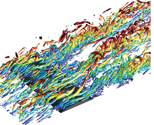
The analysis of the present flow will focus on several perspectives that have received less attention in previous studies, aiming at revealing the mechanisms underlying the separation–rotation interaction, and providing insights into the control, optimization and modelling of separating rotating flows. First, we will provide evaluations on performance modulation, i.e. variation in drag, which are of great importance to engineering applications. Second, the stability regimes have shown great success in revealing the mechanisms of turbulence modulation in rotating flows with one-dimensional velocity gradients. However, previous studies on separating rotating flows have primarily reported the 2-D distribution without establishing a connection to the spatial distribution of Reynolds stresses. Our investigation seeks to bridge this gap. Third, although several types of flow structures have been identified and analysed in conventional rotating flows, their roles in a separating setting are not well characterized or understood. There are four key structures that have the potential to interact in a rotating separating flow: (1) TG vortices due to rotation; (2) spanwise-oriented roller vortices generated by Kelvin–Helmholtz instability in the SSL (Comte, Lesieur & Lamballais Reference Comte, Lesieur and Lamballais1992; Rogers & Moser Reference Rogers and Moser1992); (3) hairpin vortices known to exist in wall-bounded turbulence (Zhou et al. Reference Zhou, Adrian, Balachandar and Kendall1999; Adrian Reference Adrian2007); and (4) oblique waves and associated  $\varLambda$-shaped vortices present on the cyclonic side (Brethouwer et al. Reference Brethouwer, Schlatter, Duguet, Henningson and Johansson2014; Brethouwer Reference Brethouwer2016). The interactions of these structures are physically responsible for the modulation of the stability regimes and Reynolds stresses. Lamballais examined the instantaneous structures and vortex lines to characterize these vortices (Lamballais Reference Lamballais2014). Streamwise-oriented, elongated structures were considered to be responsible for enhanced mixing across the shear layer and the observed early reattachment. On the cyclonic side, organization of 2-D, spanwise-oriented structures were considered as signs of stabilized SSL resistant to 3-D breakdown (Lamballais Reference Lamballais2014). We aim to characterize the structural evolution of these vortices in more depth to provide physical insights on stability and variation of the turbulent statistics.
The paper is organized as follows. First, we describe the flow configuration and numerical methods in § 2. Modulation of the mean flow, separation point and separation region is analysed in § 3, and associated changes in form drag and skin friction are assessed in § 4. The mean momentum budget is used in § 5 to justify the effects of rotation on the onset of separation. Reattachment and flow recovery are analysed using Reynolds stresses in § 6. The production of Reynolds stresses is used to interpret the role of the absolute vorticity ratio in § 7, with full budgets presented in § 8. The characterization of turbulent structures, their interaction, and their effect on the observed flow behaviour is given in § 9. Finally, we summarize and discuss implications of our findings in § 10.
2. Methodology
2.1. Simulation configuration
Turbulent channel flows rotating in the spanwise direction at Reynolds number  ${Re_b := U_b H/\nu = 2500}$ (where $H$ is the channel half-height and $U_b$ is the bulk velocity) are simulated by DNS. The friction Reynolds number $Re_\tau := u_\tau H/\nu$ is 160 when the channel is not rotating. A 2-D bump defined by the parabolic formula (normalized by $H$)
$H$)
 \begin{equation} y = \max[{-}a(x-4)^2 + h,0] - 1 \end{equation}
is placed on the bottom wall of the channel at  $y=-H$ (see figure 2a). Depending on the sign of the rotation rate, this side is either anti-cyclonic (i.e. $Ro_b >0$) or cyclonic ( $Ro_b<0$). The height of the bump is set to be $h=0.25H$. The parameter $a=0.15$ yields a bump with streamwise length $2.58H$ along the wall (i.e. $x/H=[2.71,5.29]$). These dimensions are chosen for two reasons. First, the blockage in the wall-normal direction is relatively low, and the rate of contraction/expansion is gradual. Compared with the Gaussian-shaped Boeing bump (Balin & Jansen Reference Balin and Jansen2021; Uzun & Malik Reference Uzun and Malik2022), for example, the relatively large length-to-height ratio of the current bump has several advantages for this study: (1) the favourable pressure gradient caused by the contraction at the windward side of the bump is mild such that flow is not relaminarized (Yuan & Piomelli Reference Yuan and Piomelli2011); (2) the APG at the aft part of the bump is mild (figure 2b) such that the separation point is non-fixed. The second reason for using $h=0.25H$ is that the flow up to the height of the bump will be in the destabilized (stabilized) region under anti-cyclonic (cyclonic) rotation. This will be shown in § 7.

Figure 2. (a) Bump profile and (b) inviscid streamwise pressure gradient along the surface. The profiles for the Gaussian-shaped bump used in Balin & Jansen (Reference Balin and Jansen2021) and Uzun & Malik (Reference Uzun and Malik2022) are scaled to the same height as the current bump for comparison. ![]() indicates current parabolic bump;
indicates current parabolic bump; ![]() indicates Gaussian bump.
indicates Gaussian bump.
Five cases corresponding to rotation numbers  $Ro_b = 0$, $\pm 0.42$ and $\pm 1.0$ were performed. The cases are named ‘P/NXX’ where P or N denotes positive or negative $Ro_b$, while $\text {XX}=04$ denotes $|Ro_b|=0.42$, and $\text {XX}=10$ denotes $|Ro_b|=1.0$. The non-rotating case is denoted as case 00. Cases P04 and P10 will be referred to as the ‘positive-rotating’ or ‘anti-cyclonic’ cases interchangeably. Conversely, cases N04 and N10 will be referred to as ‘negative-rotating’ or ‘cyclonic’ cases. The simulation parameters for each case are summarized in table 1. Note that the description and discussion in this paper are limited to the selected rotation rates. Terms describing the trends with respect to the rotation rate, such as ‘(non-)monotonic’, are used with respect to the tested rotation rates. They have no implication on the trends occurring between the current rotation rates and the ultimate 2-D laminar dynamics (thus 2-D laminar separation) at sufficiently high rotation rates (Grundestam et al. Reference Grundestam, Wallin and Johansson2008a; Brethouwer Reference Brethouwer2017).
Table 1. Simulation parameters:  $Re_{\tau,c}$ is the friction Reynolds number at the bump crest; $Re_{\tau,u}$ ( $Re_{\tau,s}$) is the friction Reynolds number for the anti-cyclonic (cyclonic) side of the channel; $Re_{\tau }$ is the friction Reynolds number in the fully recovered channel section; $Ro_{\tau } := 2\varOmega H/u_\tau$ is the friction rotation number in the fully recovered channel section; $x_{sep}$ is the streamwise location of the mean separation point; $y_{sep}$ is the wall-normal location of the mean separation point (relative to the bottom wall); $L_{sep}$ is the streamwise length of the mean separation bubble; and $F_D$ is the total mean drag per unit span over the entire channel. Here, $x_{sep}$, $y_{sep}$ and $L_{sep}$ are normalized by $H$, and $F_D$ is normalized by $HU_b^2$. We write $\Delta y^+_{(1)}$ for the wall-normal grid spacing in wall units at the first point from the bottom wall.

A computational domain of  $39H \times 2H \times 6H$ in the streamwise ( $x$), wall-normal ( $y$) and spanwise ( $z$) directions is employed. The long computational domain in the streamwise direction is used to ensure that the channel is well recovered near the outlet, as a streamwise-periodic boundary condition is employed. This allows for a complete examination of the recovery of the wake flow and avoidance of auxiliary boundary conditions for generating physical rotating turbulence at the inflow. In previous studies, it is reported that a flow without spanwise rotation is well recovered after 30 times the height of an obstacle (Castro Reference Castro1979; Le, Moin & Kim Reference Le, Moin and Kim1997; Song, DeGraaff & Eaton Reference Song, DeGraaff and Eaton2000; Mollicone et al. Reference Mollicone, Battista, Gualtieri and Casicola2017). In the rotating BFS study performed by Barri & Andersson (Reference Barri and Andersson2010), they showed that the mean skin friction coefficient gradually approached a constant level but was not completely recovered by 32 step heights. The length of the domain in this study is greater than 130 bump heights. It is carefully justified that not only the first-order mean quantities but also the higher-order statistics are well developed when the flow approaches the outflow boundary. An auxiliary simulation of case N04 (the slowest case to recover from the bump wake, see figure 9) was performed with an extended streamwise length $L_x = 100H$. The mean separation point, reattachment point and separation length change by less than $0.01H$ compared with the current domain. In the rear part of the SSL where fluctuations are the most prominent, the Reynolds stresses differ by less than 3 %. These minor discrepancies further indicate that the current domain length is sufficient. A periodic boundary condition is also employed in the spanwise direction. For the remaining boundary conditions, the no-slip condition is enforced along the bottom and top walls, including the bump surface.
2.2. Numerical methods
Incompressible Navier–Stokes equations for a Newtonian fluid, non-dimensionalized by  $U_b$ and $H$,
$H$,
 $$\begin{gather} \frac{\partial u_i}{\partial x_i} = 0, \end{gather}$$
 $$\begin{gather}\frac{\partial u_i}{\partial t} + \frac{\partial}{\partial x_j}(u_iu_j) ={-}\frac{\partial p}{\partial x_i} + \frac{1}{Re_b}\,\nabla^2u_i - Ro_b\,\epsilon_{i3k} u_k + f_i, \end{gather}$$
are solved by DNS. Here,  $p$ is the modified pressure, and $Ro_b$ is the bulk rotation number. The term $f_i$ is used to enforce the no-slip boundary conditions on the bump, which is achieved by an immersed boundary method (IBM) based on a volume-of-fluid (VOF) approach (Peskin Reference Peskin1972; Scotti Reference Scotti2006). The fraction of cell volume that is occupied by the fluid, denoted as $\phi$, is calculated analytically in a pre-processing calculation using the simulation grid. During the simulation, the velocity in the cells that are occupied partially or fully by the solid is weighted by $\phi$ through term $f_i$. This method has been used extensively (Scotti Reference Scotti2006; Yuan & Piomelli Reference Yuan and Piomelli2014a,Reference Yuan and Piomellib; Wu, Banyassady & Piomelli Reference Wu, Banyassady and Piomelli2016; Wu & Piomelli Reference Wu and Piomelli2018; Wu et al. Reference Wu, Piomelli and Yuan2019; Savino, Yeom & Wu Reference Savino, Yeom and Wu2023b) in the investigations of flow around embedded objects.
A Cartesian grid is designed such that the bump surface and the wake of the bump are well resolved. The grid is uniform in the  $x$ direction around the bump and in the far wake (i.e. $\Delta x/H = 0.011$ for $x/H=[2.09,6.68]$ and $\Delta x/H = 0.053$ for $x=[12, 39]$), while being stretched between $x/H = [0, 2.09]$ and $x/H =[6.68, 12]$ to transition from the two uniform spacings. The grid is also uniform in the $y$ direction below the crest with a hyperbolic tangent stretching towards the centreline. The grid is uniform in the $z$ direction. The maximum stretch ratio is less than 3 % in all directions. The grid in the $x$–
$x$– $y$ plane is shown in figure 3 for reference.

Figure 3. Computational grid in the  $x$–
$x$– $y$ plane. Every fifth grid cell is shown in both directions for clarity. The main figure is limited to $x/H=[0, 10]$, and the inset is limited to $x/H=[2.5, 5.5]$, $y/H=[-1, -0.7]$ for clarity. The bump surface is shown by the red solid line.
Two grids are tested for grid convergence. The first grid, denoted as grid I, consists of  $1196 \times 192 \times 184$ grid points in the streamwise, wall-normal and spanwise directions, respectively. For all the five cases using grid I, the maximum $\Delta x^+$ and $\Delta z^+$ near the two walls are 9.3 and 6.5; $\Delta y^+$ at the first cell from the bottom wall is reported in table 1. Because the $y$ grid is uniformly spaced to the bump crest, $\Delta y^+ < 1$ is maintained along the bump and in the wake. Away from the wall, grid I gives $\Delta h/\eta \le 6 \ (\Delta h = \sqrt{\Delta x^2 + \Delta y^2 + \Delta z^2})$, which is much smaller than the length scale at which the maximum dissipation occurs, $24\eta$ (Pope Reference Pope2000). Thus grid I is expected to be capable of resolving a substantial portion of the dissipation spectrum. Nevertheless, a finer grid (grid II) is employed for the P04 case to verify the grid convergence. This case is chosen because the moderate rotation rate leads to the greatest increase in turbulence intensity on the anti-cyclonic wall. Grid II consists of $1584\times 239\times 288$ grid points in the $x$,
$x$,  $y$ and $z$ directions, which corresponds to a refinement factor of $132\,\% \times 125\,\% \times 157\,\%$. The mean streamwise velocity and TKE are compared at selected streamwise locations in figure 4. The agreement indicates that the solutions on both grids are grid-independent. In the following, only the results calculated using grid I are shown.

Figure 4. Comparison of mean streamwise velocity and TKE at  $x/H=2$, 4, 5.5, 8 and 20, case P04.
 ![]() indicates grid I (coarser one);
indicates grid I (coarser one); ![]() indicates grid II (finer one). Each profile is shifted to the right by 2 units for
indicates grid II (finer one). Each profile is shifted to the right by 2 units for  $U$, and by 0.1 units for TKE, for clarity.
The equations of motion are solved using a well-validated finite difference code (Keating et al. Reference Keating, Piomelli, Bremhorst and Nešić2004; Wu et al. Reference Wu, Banyassady and Piomelli2016, Reference Wu, Piomelli and Yuan2019; Wu & Piomelli Reference Wu and Piomelli2018; Savino, Patel & Wu Reference Savino, Patel and Wu2023a; Wu & Savino Reference Wu and Savino2023) which solves (2.2) and (2.3) on a staggered grid. The code is second-order accurate in both time and space: a second-order-accurate central differencing scheme is used for all spatial derivatives. A second-order-accurate semi-implicit time advancement method is employed in which the Crank–Nicolson scheme is used for the wall-normal diffusion terms, while the Adams–Bashforth scheme is applied to all remaining terms. The Poisson equation is solved directly via a pseudo-spectral method (Moin Reference Moin2010) using the blktri matrix solver from the FISH-PACK software library in which a generalized cyclic reduction algorithm is employed (Sweet Reference Sweet1974; Swarztrauber & Sweet Reference Swarztrauber and Sweet1979). The code is parallelized using the message-passing interface (MPI) protocol. After each case reaches its statistically steady state, the 3-D flow field data is saved at time interval  $\delta t = 5H/U_b$ over a total $400H/U_b$ (1600 $h/U_b$) for statistical averaging. The 2-D slides of the flow field are also sampled at several planes every 115 time steps ( ${\sim }0.17H/U_b$), and history profiles of the velocity are monitored at every time step at selected locations. Statistical averages are performed in time and over the homogeneous spanwise direction. The mean quantities are denoted by capital letters or by operator $\bar {(\, \, )}$. The superscript $+$ denotes quantities scaled with the wall units. Results in the near wake of the bump will be focused on, and the region far downstream will not be shown unless necessary.
2.3. Validation
The convergence of the statistics is ensured by checking that the mean velocity and Reynolds stresses obtained using only half of the sample are within 1 % of the values calculated using the entire sample (analysis not shown for brevity). The mean velocity profiles in the fully recovered region ( $x/H=[28,31]$) are shown in figure 5. Figure 5(a) shows the mean streamwise velocity scaled in outer units. As shown by the dash-dotted lines, the expected region of $\partial U/\partial y = 2\varOmega$ is captured for both moderate and high rotation rates. Figure 5(b) shows the mean streamwise velocity scaled with wall units. Case 00 is compared with the DNS of Lee & Moser (Reference Lee and Moser2015) at $Re_{\tau } = 180$. Despite slight differences in Reynolds number, the data collapse well. Note that $Re_{\tau }$ differs on the anti-cyclonic and cyclonic walls for the rotating cases (see table 1). Thus the top and bottom portions of the channel are normalized with $Re_{\tau,s}$ and $Re_{\tau,u}$, respectively. The near-wall flow collapses on the linear law of the wall for the viscous sub-layer, indicating the sufficient resolution of near-wall turbulence regardless of modulation in turbulence intensity. Additionally, in the outer layer, the anti-cyclonic side displays a downshift compared to the canonical logarithmic relation, while the cyclonic side displays a parabolic laminar profile. This is consistent with the behaviour observed in the studies of Watmuff, Witt & Joubert (Reference Watmuff, Witt and Joubert1985), Tafti & Vanka (Reference Tafti and Vanka1991), Kristoffersen & Andersson (Reference Kristoffersen and Andersson1993) and Wu et al. (Reference Wu, Piomelli and Yuan2019).

Figure 5. (a) Mean streamwise velocity scaled with outer units. Dot-dashed lines representing  $\partial U/\partial y = 2\varOmega$ are shown for each case. (b) Mean streamwise velocity scaled with wall units. Note that for the rotating cases, the anti-cyclonic and cyclonic walls are scaled with their respective friction velocity. Case 00 is compared with DNS data from Lee & Moser (Reference Lee and Moser2015). In both plots, profiles are averaged in the streamwise direction in the range $x/H = [28,31]$.
3. Mean flow modulation: separation bubble
Mean streamwise velocity contours are shown in figure 6. Mean separating streamlines, velocity profiles at select streamwise locations ( $x/H = 4.0, 5.5, 6.0, 8.0, 12.0$), and linear plots corresponding to $\partial U / \partial y = 2\varOmega$ are superimposed. The separation (reattachment) point is defined as the streamwise location on the bump or wall where $C_f = 0$ and $\partial C_f / \partial x < 0$ ( $\partial C_f / \partial x > 0$). Note that the mean separation region is very close to the spanwise-averaged instantaneous one for the non-rotating and anti-cyclonic cases. The mean reattachment point in the cyclonic cases differs from the instantaneous passage of large coherent vortices, yet the stationary separation point remains a good representation. When subject to rotation, the velocity profiles display asymmetry about the centreline of the channel, with the development of a clear linear region. As expected, the peak velocity shifts nearer to the cyclonic side of the channel, and the magnitude of the peak velocity increases with the rotation rate. The linear region ( $\partial U/\partial y \approx 2\varOmega$) develops on the respective anti-cyclonic side of the channel. For the anti-cyclonic cases, the greatest deviation of the linear region occurs over the bump crest. For the cyclonic cases, the bump is exposed to quasi-laminar flow represented by the parabolic velocity profile. The constant velocity gradient region now on the opposite side of the bump appears minimally affected by the bump and separation region.

Figure 6. Mean streamwise velocity contours. ![]() indicates mean streamwise velocity profiles at
indicates mean streamwise velocity profiles at ![]() , 5.5, 6, 8, and 12;
, 5.5, 6, 8, and 12; ![]() indicates separating streamlines;
indicates separating streamlines; ![]() indicates velocity gradient (
indicates velocity gradient ( $\partial U/\partial y$) corresponding to $2\varOmega$. From top to bottom: $Ro_b=0$, 0.42, 1.0, $-$0.42, $-$1.0.
The skewed velocity profiles indicate that the mean flow that is subjected to the APG and separation differs between cases. A reduced velocity, i.e. mean momentum deficit (MMD), in the vicinity of the bump in the rotating cases is observed when compared to case 00. This is evident in observing the near-wall region of the velocity profiles at  $x=4.25H$ (prior to separation), as shown in figure 7(a). Because separation occurs when the near-wall fluid is decelerated to zero velocity, the increased MMD indicates that the rotating cases may separate earlier than case 00. However, our data show that this intuitive assumption is not sufficient for predicting the deceleration, separation onset and separation size. As is clearly observable in figure 6, when on the anti-cyclonic side, the separation region experiences a notable reduction in size, accompanied by a decrease in the magnitude of reverse flow as compared to the non-rotating separation bubble. Conversely, when the separation bubble is on the cyclonic side, both the size of the bubble and the magnitude of the reverse flow exhibit an increase compared to the non-rotating case. For the tested rotation rates, these trends exhibit monotonic behaviour as the rotation rate increases.

Figure 7. (a) Near-wall mean streamwise velocity profiles upstream of separation ( $x=4.25H$). Note that the wall is located at $y=-0.76H$ at this streamwise location. (b) Mean separating streamlines plotted from the separation point. The $y$-axis is stretched by a factor of 2 for clarity. Note the difference between the $y$-axis scales in (a) and (b). The legend correlating line colour and case is given in (b).
The changes at the lower rotation rate are consistent with Barri & Andersson (Reference Barri and Andersson2010), Visscher & Andersson (Reference Visscher and Andersson2011) and Lamballais (Reference Lamballais2014). However, at higher rotation rates, Lamballais (Reference Lamballais2014) reported a non-monotonic behaviour in that, compared with moderate rotation rates, the size of the separation bubble increases on the anti-cyclonic side and decreases on the cyclonic side. A significant discrepancy between Lamballais (Reference Lamballais2014) and the current work is that the separation in the former's sudden expansion channel was triggered by the fixed corner of the expansion. Therefore, the inertia of the incoming fluid dictated a minimum separation region size despite modulation in flow conditions due to rotation. In the current study, the mild surface curvature (without an abrupt geometric change) and associated mild APG allow for a variable separation point, resulting in increased freedom of the separation region to be affected by the rotation. Therefore, the reduction of the separation region in cases P04 and P10 of this study represents the effect of anti-cyclonic rotation on pressure-induced, non-fixed separation.
To assess how the variable separation point is affected by rotation, the mean separating streamlines of the five cases are superposed in figure 7(b). For reference, separation point, reattachment point and separation bubble length are listed in table 1. Compared with the non-rotating case, cases P04 and P10 show a delayed onset of separation. Conversely, the flows in cases N04 and N10 separate earlier. When subject to positive rotation as the rotation rate increases, the separation point is further delayed. When subject to negative rotation, however, the separation point does not move further towards the bump crest. The observed changes in separation point challenge the intuitive assumption that separation onset is directly correlated to MMD, a metric that is often used for pre-separation characterization (Simpson Reference Simpson1989; Greenblatt & Wygnanski Reference Greenblatt and Wygnanski2000). The flows in question have varying MMDs that do not indicate the separation location, thus a single parameter alone is not sufficient to determine the behaviour of the separation point. As shown in figure 7, case P10 displays the largest MMD yet separates the latest. The MMD of case N10 is greater than that of case N04; however, their separation points are identical.
The reattachment point also varies between cases, as shown in figure 7(b). The flow reattaches earlier when subject to positive rotation, and later when subject to negative rotation. These behaviours are monotonic (for the tested rotation rates) with an increasing rotation rate. Despite it appearing that earlier separation is correlated with later reattachment (and vice versa), this is not the sole relationship; the observed variation of the reattachment point with the rotation rate is present despite separation occurring at the same location in the negative-rotating cases. The reattachment behaviour differs from the existing literature at high rotation rates, such as Lamballais (Reference Lamballais2014), who reported later (earlier) reattachment when subject to anti-cyclonic (cyclonic) rotation at  $Ro_b = 1.0$ compared to $Ro_b = 0.33$.
The preceding observations show that despite an MMD in all rotating cases due to the skewed velocity distributions, this change alone is not sufficient to predict separation and reattachment. Other mechanisms play important roles as well. When comparing flows with the same MMD, for example, turbulent mixing is often used to justify changes in separation points. Additionally, using MMD to predict separation implicitly assumes that the main decelerating force, i.e. the streamwise pressure gradient ( $\partial P/\partial x$), does not change with the separation region. However, this may be applicable only to external flows. In confined, internal flows, the pressure gradient is inevitably significantly altered with the separation through inviscid coupling. We will further investigate the onset of separation in § 5, and reattachment in §§ 6 and 9. Before identifying the responsible mechanisms, we first discuss the performance changes of practical relevance to engineering applications.
4. Performance metrics
4.1. Total drag
Using the VOF IBM, the force exerted on the fluid to enforce the no-slip condition by the bump is calculated during every time iteration. This force contains both the frictional and form drag components produced by the bump. Integrating this force along with the wall-shear stress on the planar walls provides the total drag of the channel. The conventional notion regarding the relation between flow separation and form drag is that larger separation implies larger form drag, and vice versa. The results below show that this intuition can be misleading.
The total drag per unit span is compared in figure 8, decomposed into four sources: the friction drag produced by the bottom wall (excluding the bump),  $F_{D,{bot}} = \int \tau _w(x,-H) \,{{\rm d}\kern 0.06em x}$; the friction drag produced by the top wall, $F_{D,{top}} = \int \tau _w(x,H) \,{{\rm d}\kern 0.06em x}$; the drag produced on the wind side of the bump, $F_{D,{wind}} = \int _{-H}^{H}\int _{{LE}}^{x_c} F_1 \,{{\rm d}\kern 0.06em x}\, {{\rm d}\kern 0.05em y}$; and the drag produced on the lee side of the bump, $F_{D,{lee}} = \int _{-H}^{H}\int _{x_c}^{{TE}} F_1\, {{\rm d}\kern 0.06em x}\, {{\rm d}\kern 0.05em y}$. Here, LE, TE and $x_c$ correspond to the streamwise locations of the bump leading edge, trailing edge and crest, respectively, and $F_1$ is the mean IBM force from (2.3) in the streamwise direction. For cases P04 and P10, the bottom wall skin friction (blue bar) and the drag produced by the bump (green and red bars) sum to the total drag on the anti-cyclonic side (hatched regions). In cases N04 and N10, the friction on the top wall (orange, hatched bar) is solely responsible for anti-cyclonic side drag production. Note that the total drag (sum of these four terms) is given in table 1.

Figure 8. Total drag per unit span. The bars are split into drag produced on the bottom wall ( $F_{D,{bot}}$), top wall ( $F_{D,{top}}$), wind side ( $F_{D,{wind}}$) and lee side ( $F_{D,{lee}}$) of the bump, as shown in the legend. The inset compares the drag produced by the wind and lee sides of the bump. In all plots, hatched regions represent drag produced on the anti-cyclonic side of the channel.
All rotating cases exhibit a decrease in total drag compared to case 00. In the current configuration, the modulation of skin friction along the walls appears to contribute most significantly to the change in total drag, given that the length of the channel is considerably longer than the bump (which occupies  $7\,\%$ of a single wall). The primary contributor to the total drag decrease is the reduction in skin friction along the cyclonic wall (orange bars for cases P04 and P10, blue bars for cases N04 and N10), a consequence of diminished turbulence intensity due to relaminarization by the cyclonic rotation. Conversely, the skin friction on the anti-cyclonic wall changes non-monotonically with $Ro_b$ (hatched bars). At the moderate rotation rate (P04 and N04), skin friction on the anti-cyclonic wall is increased, counteracting the drag reduction on the cyclonic side and thus leading to a minor net reduction in total drag. At the high rotation rate (P10 and N10), the skin friction on the anti-cyclonic wall is lower than in the non-rotating case, resulting in a drastic total drag decrease together with the laminar opposite side. The suppression of turbulence and the associated drag over the anti-cyclonic wall at high rotation rates is consistent with the observations in the attached rotating flow studies of Johnston et al. (Reference Johnston, Halleen and Lezius1972) and Brethouwer (Reference Brethouwer2017).
Compared to the total drag differences, the drag produced solely by the bump differs little between all cases despite the significant change in the size of the separation region. The bump-produced drag is dominated by the positive wind-side force (drag, green bars) compared to the negative lee-side force (thrust, red bars). This behaviour is better illustrated by the inset of figure 8, where the bump-produced forces are compared directly. The predominant change by rotation is the decrease in drag on the wind side of the bump rather than the thrust on the lee side. It is found that the decrease in wind-side drag follows the same trend as the incoming MMD. Phenomenologically, this is expected, as a higher (lower) incoming velocity will result in a larger (smaller) increase of the stagnation pressure at the wind side of the bump. Case 00 displays the largest incoming velocity, and consequently the largest wind-side drag. Case P10, with the lowest incoming velocity, produces the least wind-side drag. The negative force on the lee side is often considered as a ‘back-pressure’ whose recovery depends on the size of the separation region. That is, a smaller recirculation region is expected to result in a greater back-pressure (i.e. more negative). Our results support this trend in general, with the exception being that case P04 has a similar  $F_{D,{lee}}$ to case 00, yet a smaller separation region. The variation of back-pressure between the four rotating cases, nevertheless, is small compared with that of the wind-side drag, and the latter remains the dominant contributing force. Therefore, the variation of separation size contributes little to the change in bump-produced drag. These observations indicate that the size of the separation region is not a proper indicator of the drag, even locally around the bump, at least for the current rotating configuration in question.
4.2. Skin friction on the channel walls
Because the skin friction on the channel walls is found to be the dominant term contributing to total drag and its variation with rotation, we now further examine its streamwise evolution associated with the separation region, wake and flow recovery. The mean skin friction coefficients ( $C_f := 2\tau _w/U_b^2$) along the bottom and top walls are shown in figure 9. Skin friction on the bump is excluded from the bottom wall drag as in the previous subsection. Integrating $C_f$ along $x$ on both walls shows that the accumulated skin friction exceeds the drag produced by the bump 6 $H$–7
$H$–7 $H$ downstream of the bump (or $\sim$25 bump heights). Therefore, unless the wall extends only over such a short distance downstream of the protrusion in physical applications, the skin friction along it during the prolonged recovery of the wake would remain the main source of total drag. This is typical, for example, when the protrusion is located near the leading edge of a turbine.

Figure 9. Skin friction coefficient along (a) the bottom wall and (b) the top wall. The skin friction over the surface of the bump is excluded from the plot.
When the flow is non-rotating (case 00), the skin friction along the bottom wall displays the expected behaviour of a separation bubble and reattaching flow. Specifically, a negative peak prior to reattachment signifies strong reverse flow in the recirculation region, while a positive peak post reattachment indicates strong forward flow. The latter is characteristic of impinging-type reattachment in which a strong mean downwash and/or rapidly decaying roller vortices strike the surface, as discussed in Le et al. (Reference Le, Moin and Kim1997) and Na & Moin (Reference Na and Moin1998). The steep separating streamline of case 00 near the reattachment point (refer to figure 7b) supports this claim. The recovery of  $C_f$ on the bottom wall takes ${\sim }20 H$ (80 bump heights). On the top wall, $C_f$ shows a variation due to the change of flow area by the bump. It reaches its peak at $x=4H$, where the crest of the bump is, and its minimum at $x \approx 7H$, slightly downstream of the reattachment point, indicating that the ‘dead fluid zone’ within the separation bubble (Na & Moin Reference Na and Moin1998) reduces the effective flow area of the channel. Following the minimum, the flow gradually recovers, attaining the recovered $C_f$ value ${\sim }15H$ (60 bump heights) downstream of the reattachment point.
When subjected to rotation, the wake of the bump on the bottom wall exhibits a negative–positive–peak pattern near the reattachment region similar to the non-rotating case. Positive rotation leads to a shorter transition between the two peaks due to the reduced separation region, and rapid recovery to a constant  $C_f$ within a few $H$ of the bump trailing edge. Note that the reduction of the recovery length is much more significant than that of the separation region. This indicates that rotation modulates not only the mean separation region but also the reattached flow. The non-monotonic change of the skin friction on the anti-cyclonic side in figure 8 is quantified in figure 9 as a significant plateau that is attained at a higher (lower) $C_f$ for case P04 (P10) than for case 00. This is consistent with Brethouwer (Reference Brethouwer2017) (among others), who notes a reduction in skin friction on the anti-cyclonic wall beyond $Ro\approx 0.45$. Negative rotation, on the other hand, attenuates the peaks near reattachment. This indicates that the reattachment at the end of the long separation bubbles of cases N04 and N10 is characterized by diffusion and mild impingement compared to the former cases. As shown in figure 7(b), the separating streamlines indeed exhibit more mild curvature than the positive-rotating cases. Comparing cases N04 and N10, the positive peak after reattachment is negligible at the higher rotation rate, thus $C_f$ reaches its asymptomatic value shortly downstream of reattachment. In case N04, conversely, the recovery of $C_f$ is significantly slower, such that the wake persists downstream until $x\approx 32H$. Along the top, planar wall, the streamwise variation of $C_f$ due to the bump blockage remains similar among most cases, with a shift in the asymptotic value to which $C_f$ recovers in each case. Again, $C_f$ is reduced (increased) when the top wall is the cyclonic (anti-cyclonic) wall during rotation. In the study of a rotating BFS by Barri & Andersson (Reference Barri and Andersson2010), an additional laminar separation bubble is observed on the cyclonic, planar wall opposite the step. This does not occur in the positive-rotating cases with the current configuration. Rather, $C_f$ remains positive at its minimum when the flow mildly expands over the bump and the SSL.
5. Onset of separation: mean momentum budget
As discussed previously, separation cannot be characterized by the MMD of the incoming flow alone. Rather, many factors – including spatial acceleration, turbulent mixing, APG and Coriolis effects – must be considered. We use the mean momentum budgets here to quantify why the mean separation point changes as observed. The mean momentum equation, considering a homogeneous span, reads
 \begin{equation} A_i ={-}\frac{\partial P}{\partial x_i} + D_i + R_i + G_i + F_i,\quad i=1,2. \end{equation}
The left-hand side is the mean convection ( $A_i$) arising from the material derivative of the mean velocity. The terms on the right-hand side are the mean pressure gradient ( $-\partial P/\partial x_i$, note that this term includes the driving pressure gradient $-\delta _{i1}\,\Delta P/L$ in (2.3)), mean viscous diffusion ( $D_i$), mean Reynolds stress divergence ( $R_i$), mean Coriolis force ( $G_i$), and mean IBM force ( $F_i$). Individual term definitions are provided in Appendix A. Negative values of the terms on the right-hand side correspond to decelerating flow, tending towards separation. Conversely, positive values accelerate the flow, promoting it to stay attached.
The streamwise momentum budgets at  $x=4.25H$, just upstream of the separation point for all cases, are shown in figure 10. We will focus on the wall-normal position of the peak magnitude of $A_x$ in figure 10, occurring ${\sim }0.06H$ above the bump surface. The mean velocity shown in figure 7(a) can be used as a reference for the MMD (i.e. the ‘baseline’ mean flow that is subjected to the effects of the terms on the right-hand side of (5.1)). When the channel is not rotating, the streamwise deceleration is caused primarily by the APG (figure 10, case 00). For anti-cyclonic rotation (cases P04 and P10), $G_x <0$ as the mean flow tends to follow the lee-side contour of the bump ( $V<0$); however, this is not a leading term in the budget. The magnitude of the APG decreases significantly; meanwhile, the magnitude of the Reynolds stress divergence increases (note that this term corresponds to both the generation and diffusion of TKE and thus should not be interpreted solely as a change in the magnitude of turbulent fluctuations). Consequently, the magnitude of $A_x$ decreases in the anti-cyclonic cases, representing less deceleration. This compensates for the incoming MMD, and ultimately delays separation. Thus the delayed separation is not a direct consequence of the Coriolis force, but rather the indirect reduction of APG and increase of Reynolds stress divergence by rotation.

Figure 10. Mean streamwise momentum balance terms at  $x=4.25H$ (refer to (5.1)). The plots represent individual cases as denoted by case name labels. Here, $-\partial P/\partial x$ is the mean streamwise pressure gradient, $G_x$ is the mean streamwise Coriolis force, $R_x$ is the Reynolds stress divergence, $A_x$ is the mean streamwise advection, and $D_x$ is the viscous diffusion. All quantities are normalized by $U_b^2/H$. Note that the profiles begin from the height of the bump at $x=4.25H$ ( $y=-0.76H$).
Under cyclonic rotation (cases N04 and N10), the Coriolis term ( $G_x$) is expected to be positive on the lee side of the bump (since $V<0$ and $\varOmega <0$) and delay separation. This is observed near the bump surface; however, it is weaker than the negative $G_x$ term that promotes separation in P04 and P10. Further away from the bump, it becomes negative as the mean downward flow along the bump diminishes. Therefore, the Coriolis force is not directly responsible for the early separation in the cyclonic cases. Furthermore, the streamwise APG, as the major decelerating force, is reduced compared to the non-rotating case. While the above trends indicate that flow should remain attached longer, the Reynolds stress divergence diminishes as the flow tends to relaminarize. Thus no turbulence is present to transport high momentum towards the bump as in the other three cases. Therefore, despite the deceleration ( $A_x$) being smaller compared to case 00, it is still sufficient such that the MMD is brought to separation earlier than in the non-rotating scenario. Overall, the $x$ momentum balance shows that the early separation in the negative-rotating cases is because of the MMD and lack of turbulence, despite the weakened decelerating force. Again, it must be recalled that the relaminarization and thus early separation is an indirect consequence of the Coriolis force under cyclonic rotation. That said, any flow control approach that imparts a mean $V<0$ will render the Coriolis term as a direct contributing factor to delay cyclonic flow separation.
The need now arises to determine why the rotation leads to reduced APG and modulated Reynolds stress divergence. Considering first the APG, this can be explained by a bulk estimation of the pressure gradient based on Bernoulli's equation and conservation of mass:
 \begin{equation} \frac{\partial{P}}{\partial {x}} ={-}U\,\frac{\partial{U}}{\partial {x}} \propto \frac{U}{A^2}\,\frac{\partial{A}}{\partial {x}}, \end{equation}
where  $A$ denotes the channel area varied along the bump. From (5.2), it is clear that the APG will be lower if the mean $U$ is smaller over the lee side. Indeed, the variation of APG is correlated to that of the MMD (see figure 7a). Specifically, the stark decrease in velocity in the anti-cyclonic cases is reflected in the decrease of APG. Therefore, the skewed mean velocity profile induced by the rotation results in decreased APG, thus less decelerating force in the rotating cases.
6. Turbulence statistics: Reynolds stress distributions
As the above discussion highlights, the Reynolds stress divergence has a significant influence on the mean separation point. Therefore, we now analyse the Reynolds stress distributions to further understand the effect of the turbulence modulation by rotation. Contours of the Reynolds normal stresses ( $\overline {u'u'}, \overline {v'v'}$ and $\overline {w'w'}$) along with the Reynolds shear stress ( $-\overline {u'v'}$) are given in figures 11–14. The solid line represents the separating streamline. As mentioned in § 1, the mean absolute vorticity ratio ( $S$) plays an important role in influencing the turbulence characteristics of rotating flows. We have thus superimposed isocontour lines $S=-1$ (dotted) and $S=-0.5$ (dash-dot), indicating expected regions of enhanced turbulence.

Figure 11. Contours of  $\overline {u'u'}$.
 ![]() indicates separating streamline;
indicates separating streamline; ![]() indicates
indicates  $S=-1.0$;
 ![]() indicates
indicates  $S=-0.5$. The $S$ contour lines at the peak streamwise velocity are not plotted for clarity. Note that the $y$-axis is stretched to improve visualization of the separation region.

Figure 12. Contours of  $\overline {v'v'}$. For line style legend, see caption of figure 11.

Figure 13. Contours of  $\overline {w'w'}$. For line style legend, see caption of figure 11.

Figure 14. Contours of  $-\overline {u'v'}$. For line style legend, see caption of figure 11.
Using case 00 as a benchmark, the onset of streamwise fluctuations ( $\overline {u'u'}$) occurs first near the separation point, while significant wall-normal ( $\overline {v'v'}$) and spanwise ( $\overline {w'w'}$) fluctuations develop downstream near the reattachment point, and $-\overline {u'v'}$ develops an appreciable magnitude at the streamwise centre of the separation bubble. These high-stress regions all occur in the forward-flow side of the SSL. The augmented stresses begin to lose intensity within a few $H$ of reattachment, displaying a nearly full recovery (i.e., little streamwise variation) by $x/H=12$. Throughout the shear layer and wake recovery, the wall-normal position of peak stresses changes little, forming a wake that extends parallel to the walls. These spatial distributions align with the established understanding of Reynolds stress distribution in APG-induced separation, representing the development of the turbulent SSL and its recovery after reattachment, as discussed in Na & Moin (Reference Na and Moin1998) (among others). On the top wall, the only notable change due to the bump is a decrease in $\overline {u'u'}$ where the flow area is reduced by the bump, an expected suppression of turbulence due to the favourable pressure gradient. Yet this effect is insignificant as the bump is designed to provide little blockage and generate mild pressure gradients.
When subject to positive rotation (cases P04 and P10), the spatial distribution of Reynolds stresses exhibits significant variations compared with case 00. Relative to the separation point,  $\overline {u'u'}$ develops appreciable values earlier than in case 00. Additionally, its region of elevated magnitude is remarkably reduced in size and confined nearer the bump surface. Similar spatial variations apply to $-\overline {u'v'}$. While the onset of $\overline {v'v'}$ also occurs earlier relative to reattachment, there is a stark increase in the size of its enhanced region when subject to positive rotation, despite the considerably smaller mean separation region in these two cases. The increase of $\overline {w'w'}$, which is conventionally used to represent the three-dimensionalization of the separated shear layer, remains highly correlated with the reattachment. However, the peak $\overline {w'w'}$ occurs near the wall rather than in the shear layer.
Another qualitative difference with the intense-stress regions from the non-rotating case is that those in the positive-rotating cases show an upward shift of their peak towards the opposite wall along the wake of the bump. This peak line does not occur along any mean streamline. This behaviour is most prominent for  $\overline {v'v'}$, in which it extends over $3H$ downstream of the bump. For $\overline {u'u'}$ and $-\overline {u'v'}$, this region rapidly diminishes approximately 0.5 $H$–1.5 $H$ downstream of the bump. For $\overline {w'w'}$, the inclined augmented region is present; however, it is not comparable in magnitude to its near-wall peak. This phenomenon has been observed in the rotating separation literature. Specifically, in the rotating sudden expansion study of Lamballais (Reference Lamballais2014), a region of augmented $\overline {v'v'}$ originating on the lee side of the anti-cyclonic separation bubble extends towards the opposite cyclonic wall, while $\overline {u'u'}$ is significantly attenuated and extends at the same angle (see Lamballais Reference Lamballais2014, figures 13d, f). An explanation for this spatial distribution was not provided, however.
We found that the discussed high Reynolds stress regions in the positive-rotating cases exhibit a correlation with the thresholds of  $S$ that differentiate the stability regimes. Specifically, the diminishing boundaries of the high $\overline {u'u'}$ and $\overline {u'v'}$ regions align surprisingly well with the $S= -0.5$ contour line, while for $\overline {v'v'}$ and $\overline {w'w'}$, there is general agreement with $S=-1.0$. Because $S$ is a representation of the interplay between the mean shear vorticity and the system rotation, the observed correlation between the Reynolds stresses and specific $S$ values suggests a strong influence of the Coriolis force on the Reynolds stresses. Additionally, the spatial sequence, with elevated $\overline {v'v'}$ and $\overline {w'w'}$ regions downstream of the peak $\overline {u'u'}$ and $-\overline {u'v'}$, implies a causal relationship between these variations. The influence of rotation on the Reynolds stresses with regard to $S$ is discussed in the next section.
Comparing the two positive-rotation rates, case P10 has significantly lower Reynolds stresses than case P04 upstream of the bump. This represents the suppressed turbulence at the high rotation rate. Similarly, in the wake of the bump,  $\overline {u'u'}$ and $-\overline {u'v'}$ are smaller in magnitude in case P10, even when compared to case 00. However, the augmentation of $\overline {v'v'}$ in the inclined region along the $-1< S<0$ region remains remarkable and more pronounced than in case P04; $\overline {w'w'}$, while qualitatively similar to case P04, exhibits a smaller magnitude in case P10.
The Reynolds stress distribution in the negative-rotating cases is much as expected. The SSL exhibits the typical features of a laminar SSL. Intense Reynolds stresses appear only considerably downstream near the reattachment point, corresponding to the formation and decay of 2-D roller vortices. The stabilization ( $S>0$) effect of the Coriolis force is evident: the stresses are much lower in case N10 than the ones in case N04. The prolonged SSLs cause an extended blockage of the channel. This leads to a slight increases of $\overline {u'u'}$ along the top, anti-cyclonic wall, followed by augmented $\overline {v'v'}$ and $\overline {w'w'}$. Importantly, the augmented stresses here are correlated with enlarged destabilized regions ( $-1< S<0$).
The Reynolds stress distributions discussed above clearly indicate correlation between turbulence generation and rotation-induced destabilized regions. Therefore, we now further investigate the influence of rotation on turbulence characteristics in the current flow.
7. Discussion on stability regimes of rotating flows
Stability analysis of various rotating shear flows has shown that the ratio of system rotation to mean shear vorticity ( $S:=\varOmega /\varOmega _s$) influences flow stability, turbulence characteristics, and coherence of large-scale structures (Hart Reference Hart1971; Yanase et al. Reference Yanase, Flores, Métais and Riley1993; Cambon et al. Reference Cambon, Benoit, Shao and Jacquin1994; Métais et al. Reference Métais, Flores, Yanase, Riley and Lesieur1995; Salhi & Cambon Reference Salhi and Cambon1997; Brethouwer Reference Brethouwer2005), as reviewed in § 1. Despite the criteria for stability of rotating flows being established for flows without spatial development, our data show a strong correlation between destabilized regimes and regions of augmented Reynolds stress in the bump wake. Therefore, we discuss the physical implication of destabilized regimes with the objective to determine why the observed correlations exist.
7.1. One-dimensional baseline state
The absolute vorticity ratio in the fully recovered region as a function of  $y/H$ and $y^+$ is given figures 15(a) and 15(b), respectively. Dotted lines at $S=-1$ and $S=0$ bound the destabilized region. As expected, flow is destabilized near the anti-cyclonic wall, above which the neutral regime corresponding to $S=-1$ and the constant velocity gradient exists. Above this, the flow is stabilized, characterized by $S<-1$ below the peak velocity and $S>0$ in the cyclonic side. The relationship between the destabilized regime and dynamically important regions of turbulent channel flow is evident when $y$ is plotted in wall units on a log scale, as shown in figure 15(b). For the moderate rotation rate, the entire inner layer of the channel, including the log-law region, is destabilized. At the high rotation rate, on the contrary, the destabilization affects only up to the lower limit of the log layer. As a result, the turbulence in the anti-cyclonic side is augmented for the entire dynamically important inner layer in cases P04 and N04, and is enhanced only near the legs of the embedded hairpin vortices in cases P10 and N10. This leads to reduced turbulence and skin friction at high rotation rates as shown in the literature (Johnston et al. Reference Johnston, Halleen and Lezius1972; Xia et al. Reference Xia, Shi and Chen2016; Brethouwer Reference Brethouwer2017).

Figure 15. Absolute vorticity ratio ( $S$) at the fully recovered region of the channel: (a) as a function of $y/H$; (b) as a function of the distance to the wall in wall units, $y^+ = y u_\tau /\nu$. Vertical dotted lines mark the stability thresholds $S=-1$ and $S=0$.
7.2. The 2-D variation of absolute vorticity ratio
Because the flow is spatially developing due to the bump and its wake, the mean shear and subsequently absolute vorticity ratio become 2-D rather than well-defined wall-parallel layers as in canonical channel flow. As seen in figures 11–14, for cases P04 and P10, a large region of destabilized flow extends from the lee side of the bump at an angle towards the channel centreline. For cases N04 and N10, an increased region of destabilized flow forms along the top wall near the streamwise reattachment location. Because change is from  $S\sim -1$ (neutral) to $S>-1$ (destabilized), this indicates that the mean shear vorticity becomes larger in magnitude than 2 $\varOmega$ in these regions. Upon examination of $\partial V/\partial x$ and $\partial U/\partial y$, it was found that the latter has a similar spatial variation as the inclined $S=-1$ contour (not shown). This is caused by the deceleration of the flow on the lee side of the bump by the APG. A reduced-velocity layer forms near the bump regardless of whether the flow separates or not (note that in case P10, the separation is minimal but the momentum deficit remains significant; see figure 7). The slow-moving layer decreases the distance over which the velocity increases to its peak, therefore increasing the velocity gradient ( $\partial U/\partial y$) and driving $S$ to the destabilized regime. For cases N04 and N10, the APG and increased $\partial U/\partial y$ behind the bump only make $S$ less positive, hence flow here remains stabilized. However, as the separating streamline curves towards the bottom wall, the effective flow area expands, inducing an APG. This increases $\partial U/\partial y$ along the top (anti-cyclonic) wall, and drives $S$ into the destabilized regime.
Therefore, it is concluded that increased  $\partial U/\partial y$, caused by deceleration of near-wall flow is responsible for the 2-D variation of increased $S$. Note that this change is highly sensitive to the mean velocity profile: referring to the mean velocity profiles for cases P04 and P10 at $x/H=5.5$, 6 and 8 in figure 6, the misalignment between the reference lines of $2\varOmega$ slope and the mean velocity is notable only to approximately the bump height, yet this slight variation into the unstable regime leads to a prominent change in $S$, and correspondingly the Reynolds stresses, up to the channel centreline.
7.3. Relationship with Reynolds stresses
It now remains to determine why such regions are correlated with augmented Reynolds stresses. Reynolds stress production terms are given in table 2. Combining mean shear and rotational streamwise production yields
 \begin{equation} P_{uu, {tot}} \approx 4\varOmega\,\overline{u'v'} - 2\,\overline{u'v'}\,\frac{\partial U}{\partial y} = 2\,\overline{u'v'}\left( 2\varOmega - \frac{\partial U}{\partial y} \right) ={-}2\,\overline{u'v'}\,\frac{\partial U}{\partial y}( S+1). \end{equation}
Here,  $\partial U/\partial x$ is considered negligible compared with the wall-normal shear. Considering the anti-cyclonic side ( $S<0$), $P_{uu,{tot}}$ is a source of $\overline {u'u'}$ when $-1< S<0$, and a sink when $S<-1$. Therefore, $S=-1$ is often identified in the literature as the delimiter between net gain of $\overline {u'u'}$ from the mean flow and loss to $\overline {v'v'}$ through rotational effects, and respectively the augmentation or suppression of turbulence. On the cyclonic side ( $S>0$), $P_{uu,{tot}}$ is a source of $\overline {u'u'}$. However, $G_{vv}<0$, signifying redistribution of TKE back to $\overline {u'u'}$ and the suppression of the turbulence generation cycle, leading to relaminarization. These mechanisms have been well characterized in the literature, and explain the general correlation between augmented Reynolds stresses and the $S=-1$ contour.
Table 2. Production and Coriolis terms in the Reynolds stress budgets.

However, less attention has been given to the  $S=-0.5$ threshold, which we have observed to be highly correlated with regions of intense $\overline {u'u'}$ and $\overline {u'v'}$. Rather than simply considering the signs of $P_{uu,{tot}}$ and $G_{vv}$, we now compare their magnitudes on the anti-cyclonic side. We have $P_{uu,{tot}} > G_{vv}$ when $S+1>-S>0$, i.e. $-0.5< S<0$. Considering further that $G_{uv}$ depends on the difference between $\overline {u'u'}$ and $\overline {v'v'}$, the greater production of $\overline {u'u'}$ versus $\overline {v'v'}$ will lead to greater magnitude $\overline {u'v'}$. The cycle is self-sustaining, with the elevated $\overline {u'v'}$ further increasing the difference between $\overline {u'u'}$ and $\overline {v'v'}$. Following the same argument, $G_{vv}>P_{uu,{tot}}$ when $-1< S<-0.5$. Here, we can expect $G_{uv}$ to decrease, ultimately resulting in $\overline {u'u'}$ being diminished. It is thereby evident why $\overline {u'u'}$ is significantly augmented within the $S=-0.5$ contour, and rapidly diminishes outside it.
We have provided mechanisms responsible for the 2-D variation of absolute vorticity ratio, and provided insight into the implications of these variations through analysis of Reynolds stress production terms. Note that while regimes from stability theory were used to guide the preceding analysis, the rigorous establishment of new regimes through stability analysis is beyond the scope of this paper. We now investigate the full Reynolds stress budgets before analysing the physical mechanisms responsible for the discussed behaviours.

Figure 16. Budgets of (a,d,g,j,m)  $\overline {u'u'}$, (b,e,h,k,n) $\overline {v'v'}$, and (c, f,i,l,o) $\overline {w'w'}$ at the respective streamwise centre of the separation bubble for each case. Note the difference in axis scaling between terms and cases.
 ![]() indicates
indicates  $y\vert _{U=0}$;
 ![]() indicates
indicates  $y\vert _{{max}(\partial U/\partial y)}$;
 ![]() indicates
indicates  $y\vert _{S=-0.5}$.
8. Reynolds stress budgets: SSL
The budgets of  $\overline {u'u'}$, $\overline {v'v'}$ and $\overline {w'w'}$ at the centre of the separation region of each case are shown in figure 16. Production ( $P_{ij}$) and Coriolis ( $G_{ij}$) terms are given in table 2, and the conventional terms are in Appendix A. Without rotation, the $\overline {u'u'}$ budget is dominated by the gain from shear production and loss through the fluctuating velocity–pressure-gradient correlation, both of which reach their peak magnitudes at the inflection point in the SSL. The latter is the primary source of $\overline {v'v'}$ and $\overline {w'w'}$. This agrees with previous studies of plane mixing layers and SSLs (Rogers & Moser Reference Rogers and Moser1994; Na & Moin Reference Na and Moin1998). When rotation is cyclonic for the flow near the bottom wall (cases N04 and N10), the budgets of the Reynolds stresses are qualitatively similar to shear-layer dominant dynamics in case 00. Note that the terms corresponding to these two cases are depicted with reduced $y$-axis ranges in figure 16 as the flow is quasi-laminarized. Here, $G_{uu}$ is extracting energy from $\overline {v'v'}$ and preventing the formation of the roller vortices in the shear layer.
When rotation is anti-cyclonic, the Coriolis term acts as a sink for  $\overline {u'u'}$ and a source for $\overline {v'v'}$, as expected. One notable change to the $\overline {u'u'}$ budget in case P04 is that the production does not occur at the inflection point in the shear layer. Rather, it appears where $G_{uu}$ reaches its peak magnitude. Examining the sub-terms of $P_{uu} = -\overline {u'u'}\,\partial U/\partial x -\overline {u'v'}\,\partial U/\partial y$, we found that both $\overline {u'u'}$ and $\overline {u'v'}$ obtain their peak magnitudes at this location, yet the mean shear peaks at the inflection point of the velocity profile nearer to the wall. This indicates that the Coriolis effect replaces the canonical shear layer mechanisms of the $\overline {u'u'}$ dynamics in this case. Referring to § 7, we notice that the peak production of $\overline {u'u'}$ is in the self-sustaining regime where $-0.5< S<0$: more energy is extracted from the mean flow to $\overline {u'u'}$ than redistributed to $\overline {v'v'}$. The increased difference between $\overline {u'u'}$ and $\overline {v'v'}$ enhances $\overline {u'v'}$, enabling the self-exciting cycle. This is further proven by our data as the magnitude of $\overline {u'v'}$ is doubled at the peak, and $\overline {u'u'}$ remains comparable to case 00 despite $\overline {v'v'}$ extracting energy from it. For $\overline {v'v'}$, the $G_{vv}$ term becomes a leading source. Similar to $\overline {u'u'}$, $P_{vv}$ is misaligned with the inflection point where the maximum shear occurs. However, it is shifted less towards the peak of $G_{vv}$ because the leading shear ( $\partial V/\partial y$) is more skewed towards the SSL than $\partial U/\partial y$ for $\overline {u'u'}$ (not shown). Another remarkable qualitative change in the $\overline {v'v'}$ budget is that the velocity–pressure correlation term becomes a sink that peaks in the vicinity of the wall. Therefore, the TKE redistribution from $\overline {u'u'}$ to $\overline {v'v'}$ and $\overline {w'w'}$ in the non-rotating case (and canonical turbulent boundary layers (TBLs)) is altered such that the fluctuating pressure extracts energy from both $\overline {u'u'}$ and $\overline {v'v'}$, and redistributes it to $\overline {w'w'}$. This modified redistribution is the most significant near the inflection point of the shear layer, where the transfer is primarily from $\overline {v'v'}$ to $\overline {w'w'}$. It leads to an increased gain in the $\overline {w'w'}$ budget compared to case 00. Summarizing the observation for all three Reynolds normal stresses, it is evident that the total gain is increased for all components compared to the non-rotating case. This is the reason for the enhanced Reynolds stresses (see figures 11–14), as well as the early reattachment observed in case P04.
At the higher positive-rotation rate, most of the terms in the  $\overline {u'u'}$ budgets reduce in magnitude. It is found that the mean shear is still substantial in the shear layer, yet the Reynolds stresses are reduced. The consequence of the decreased fluctuations is also exhibited in the $G$ terms, which are nearly equivalent to those in case P04 despite the rotation rate being more than doubled. We again refer to the discussion in § 7 to justify this change: the deceleration changed the neutral ( $S\sim -1$) region to the self-sustaining state ( $-0.5< S<0$) in case P04, yet only to $-1< S<-0.5$ where $\overline {u'u'}$ is restricted in P10. In such a region, the net $P_{uu,{tot}}$ can still extract energy from the mean flow. However, this extraction is counteracted by the Coriolis influence through $G_{uv}$. As $\overline {v'v'}$ extracts a significant amount of energy from $\overline {u'u'}$ and surpasses the latter, the $G_{uv}$ term becomes positive, mitigating the negative $\overline {u'v'}$, and resulting in a reduction of $P_{uu,{tot}}$. For $\overline {v'v'}$, the Coriolis term is now the dominant gain. Therefore, the enhanced $\overline {v'v'}$ region shown in figure 12 for case P10 is mainly through rotation. The redistribution by fluctuating pressure is now only between $\overline {v'v'}$ and $\overline {w'w'}$, likely a cause of the weakened $\overline {u'u'}$ due to extraction by $G_{uu}$.
9. Characterization of embedded structures
In this section, we aim to identify the physical processes responsible for the changes in separation point and Reynolds stresses discovered throughout the paper. Specifically, we look to the dynamic structures in the flow, i.e. the hairpin vortices of turbulence, TG vortices, roller vortices in the SSL, and the oblique waves on the stable side.
9.1. Instantaneous flow field
The small-scale structures are shown by the isosurfaces of the second invariant of the velocity gradient tensor ( $Q:= - (1/2)(\partial u_j/\partial x_i)(\partial u_i/\partial x_j)$) in figure 17. In figure 18, spanwise vorticity ( $\omega _z$) and $Q$ are extracted in the streamwise–wall-normal ( $x\unicode{x2013}y$) plane at the channel midspan to visualize the shear layer and the wall-normal distribution of the vortices. Notably, TG vortices are not able to be visualized by these quantities due to their large-scale coherence. Thus instantaneous flow fields of streamwise vorticity ( $\omega _x$) and wall-normal velocity in the cross-flow ( $z$–
$z$– $y$) plane in the wake of the bump are provided in figure 19 to visualize them. They are observed by the large-scale counter-rotating swirls, indicating alternating regions of upwash and downwash. The absence of vortices in the streamwise-elongated regions in the top view of the $Q$ isosurfaces (figure 17) serves as an additional depiction of TG vortices.

Figure 17. Isosurfaces of the second invariant of the velocity gradient tensor visualized at a level  ${Q=2.0 U_b^2/H^2}$. (a,c,e,g,i) isometric view coloured by wall-normal distance to the bottom wall ( $y/H$). (b,d,f,h,j) top view coloured by instantaneous streamwise velocity fluctuation ( $u'/U_b$). From top to bottom, rows correspond to cases 00, P04, P10, N04, N10, as in preceding figures. Note that for the anti-cyclonic cases, the circled packets of ejected hairpin vortices correspond to the TG vortex-induced upwash indicated by arrows in figure 19.

Figure 18. Contours of instantaneous flow in the channel midspan: (a) spanwise vorticity ( $\omega _z$); (b) second invariant of the velocity gradient tensor ( $Q$, see text).

Figure 19. Contours of instantaneous flow in the cross-flow plane at  $x/H=7.0$: (a) streamwise vorticity $\omega _x$; (b) wall-normal velocity and velocity vectors. The vectors are shown every $0.3H$ in $z$, and $0.1H$ in $y$, normalized by their magnitude for clarity. Horizontal lines represent (if applicable):
 ![]() $y\vert _{S=-0.5}$;
 ![]() $y\vert _{{max}(\partial U/\partial y)}$;
 ![]() $y\vert _{U=0}$. Note that for the anti-cyclonic cases, the regions of upwash indicated by arrows correspond to the regions of ejected hairpin vortices circled in figure 17.
When the channel is not rotating, a roller vortex can be seen underneath a nest of hairpin vortices in the SSL. The latter dominates the downstream region with several well-defined arched heads appearing randomly across the domain. In the positive-rotating cases, the SSL is strongly disrupted. Weakly coherent spanwise-oriented vortices in the shear layer for case P04 are highlighted in figure 17 and the spanwise vorticity contour of figure 18. It is observed that TG vortices induce spanwise variation of the separation point for the anti-cyclonic cases, as shown through instantaneous streamwise velocity on the bump along with  $z$–
$z$– $y$ planes of instantaneous wall-normal velocity in figure 20. Regions of upwash and downwash induced by the TG vortices are clearly correlated with locally separated and attached flow, respectively. The hairpin vortices in the incoming flow are elongated in the streamwise direction as shown by the $Q$ isosurfaces. They are longer and more parallel to the wall in case P10 than in P04. This agrees with the findings in the literature that rotational instability favours the growth of streamwise vortices (Lesieur, Yanase & Métais Reference Lesieur, Yanase and Métais1991; Yanase et al. Reference Yanase, Flores, Métais and Riley1993; Métais et al. Reference Métais, Flores, Yanase, Riley and Lesieur1995; Lamballais et al. Reference Lamballais, Lesieur and Métais1996), and that hairpin legs are enhanced in rotating flows (Iida, Tsukamoto & Nagano Reference Iida, Tsukamoto and Nagano2008; Yang & Wu Reference Yang and Wu2012; Brethouwer Reference Brethouwer2017).

Figure 20. Contours of instantaneous streamwise velocity on the bump surface and wall-normal velocity in the  $z$–
$z$– $y$ plane. Velocity vectors are superposed onto the $z$–
$z$– $y$ plane. Only the non-rotating and anti-cyclonic cases are displayed since the TG vortices interact with the SSL only on the anti-cyclonic side.
The wake of the bump exhibits rich dynamics represented by the evolution of the hairpin vortices. In the spanwise vorticity and  $Q$ contours at the channel midspan (figure 18), it can be seen that the series of hairpin vortices is distributed along a path that extends from the SSL towards the channel centreline. This trajectory aligns with the extended $-1< S<0$ region and where $\overline {v'v'}$ and $\overline {w'w'}$ exhibit enhancement. This trend can also be observed in the $Q$ isosurfaces (figure 17) and the cross-flow contours (figure 19), where a clear correlation of the region between TG vortex pairs (i.e. strong upwash) and the ejection of hairpin vortices can be identified. At the time instants shown in these figures, four ejection gaps can be seen in case P04, and six are visible in case P10. This agrees with the literature that TG vortices are smaller and closer to the anti-cyclonic wall at high rotation rates. Correlating the cross-flow contours, the $Q$ isosurfaces and the Reynolds stresses contours (figures 11–14), the eddies being ejected have large streamwise vorticity near the wall, thus corresponding to the legs of the hairpin vortices. The bottom of these legs creates the high $\overline {w'w'}$ in the vicinity of the wall, while their rotation appears as the strong $\overline {v'v'}$ and $\overline {u'u'}$. Beyond $y/H\sim -0.6$ to $-$0.7, the streamwise vorticity decreases, forming arched structures in the cross-flow contours. This is where the head of the hairpin is formed. The vortex filaments generated by the breakdown of the hairpin heads can be ejected up to the cyclonic side of the channel at $y/H\sim 0.5$ (refer to the 2-D $Q$ contour in figure 18). Due to the smaller TG vortices at the higher rotation rate, the width and ejection height of the hairpin vortices in the wake of the bump are smaller in case P10 than in P04.
We interpret the correlation between the  $-1< S<0$ region and the trajectory of the hairpin vortices as follows. Recall that the lee side of the bump is in the destabilized regime, as discussed in § 7. Therefore, hairpins here are ejected into a region where they are augmented and able to extract more significant energy from the mean flow (versus being ejected into a neutrally stable regime, as occurs in a planar rotating channel). Furthermore, the ejection regions between TG vortices are found to have negative $u^\prime$, as is clearly visible in the top view of the $Q$ isosurfaces. Thus the ejection mechanism is similar to the ejection events between low-speed streaks in TBLs: a local low streamwise velocity will increase the wall-normal velocity by mass conservation. However, the causation is the opposite here since the upwash generated by the TG vortex pair initiates the local deceleration. The reduced streamwise velocity increases $\partial u/\partial y$ in the wake of the bump (i.e. away from the wall). As discussed in the stability regime section (§ 7), an increased velocity gradient leads to a less negative $S$ that makes such regions unstable. The extraction of kinetic energy from the mean flow to $\overline {u'u'}$ and redistributed to $\overline {v'v'}$ via the Coriolis terms is the statistical description of the augmentation of the hairpin vortices mentioned above. Moreover, we attribute this process to the inclined extension of the destabilization region that reaches up to the channel centreline. On one hand, it can be viewed as a faster recovery of the near-wall region to the neutral $S=-1$ regime, compared to the channel centreline. On the other hand, it also represents the consequence of the continuous mean momentum extraction as the enhanced hairpin vortices are ejected. Both of these two processes are characterized by the Reynolds stress divergence in the mean momentum budget, and the production and turbulent diffusion in Reynolds stress budgets. The physical picture corresponding to this process is that as the hairpin vortices are lifted in the ejection regions, their (enhanced) legs bring high momentum to the region underneath by their rotation to facilitate the recovery of the near-wall flow. Yet they keep draining the mean momentum at their height through the Coriolis terms. Thus the region away from the wall attains a prolonged modulation. This process continues until the TG vortices cannot further sustain the ejection of the enhanced hairpin vortices, and/or the hairpin vortices break down such that they no longer extract significant energy from the mean flow.
In the negative-rotating cases, the hairpin and TG vortices are on the opposite side of the bump and do not directly impact the SSL. The  $Q$ isosurfaces show the footprints of the oblique waves on the roller vortices formed far downstream of the bump. A spanwise wavelength about half of the spanwise domain size can be seen. Case N04 exhibits significantly more distorted vortices than N10. This is consistent with the literature that turbulent spots on the stable side diminish as the rotation rate increases (Grundestam et al. Reference Grundestam, Wallin and Johansson2008a; Brethouwer Reference Brethouwer2017). Note that there are diverse opinions about the origin of these turbulent spots. Local cyclic turbulent bursts by the growth and breakdown of Tollmien–Schlichting (TS) waves, and turbulent fluctuations penetrating into the stable region, are two main mechanisms proposed (Kristoffersen & Andersson Reference Kristoffersen and Andersson1993; Brethouwer et al. Reference Brethouwer, Schlatter, Duguet, Henningson and Johansson2014; Brethouwer Reference Brethouwer2016; Dai et al. Reference Dai, Huang and Xu2016). For the flow in the current study, we are inclined to the latter because: (1) there is a prominent ejection of the hairpin vortices excited by the extended unstable region in the wake of the bump; and (2) the relatively low $Re_\tau$ and $Ro_\tau$ prevent the TS waves from reaching very large amplitude (Brethouwer et al. Reference Brethouwer, Schlatter, Duguet, Henningson and Johansson2014). The cross-flow contours of these two cases (figure 19) exhibit that the head of the hairpin vortices ejected from the opposite side indeed reaches the SSL in case N04, while it does not seem so in case N10. This is again because the TG vortices are smaller and nearer the anti-cyclonic wall as the rotation rate increases.
The dynamics of the structures elaborated above indicates that any increase in shear, whether by deceleration of near-wall flow as observed in this study, or acceleration of outer flow, will result in an increased  $\partial U/\partial y$, which increases the absolute vorticity ratio from $S\sim -1$ to $-1< S<0$. In such a region, the hairpin vortices in the boundary layer will be augmented and sustained longer as they are ejected by the TG vortices, reaching further into the core of the flow (compared with in the same rotating system under a zero pressure gradient, in which the hairpins also get ejected by the TG vortices). Therefore, this process could also occur in attached flows, including on the anti-cyclonic side of our negative-rotating cases. Indeed, we observed an increased $S$ near the top anti-cyclonic wall, and enhanced $\overline {v'v'}$ and $\overline {w'w'}$ in cases N04 and N10 (figures 12 and 13). Therefore, the turbulent patches superposed to the oblique wave and disturbing the laminar SSL in case N04 are likely energized filaments of the ejected hairpins from the opposite (attached) side. In particular, the increased $\overline {v'v'}$ and $\overline {w'w'}$ near the anti-cyclonic wall in cases N04 and N10 are most prominent not immediately downstream of the bump, but where the wall-parallel laminar shear layer starts to curve towards the wall, creating an expansion of the nominal cross-sectional area and thus an APG. This supports our claim that near-wall deceleration is what causes destabilization of anti-cyclonic flow, leading to the observed augmentation of hairpin vortices and turbulence.
9.2. Premultiplied spanwise spectrum
The spanwise wavelength and wall-normal location of the embedded structures are quantified by the premultiplied energy spectrum of velocity fluctuations in figure 21. Note that each spectrum is normalized by its peak magnitude. Without rotation, the peaks of the  $\overline {u'u'}$ and $\overline {v'v'}$ spectra collapse at the location of the inflection point, representing the generation of roller vortices. The primary wavelength is approximately $0.7H$. In wall units, it corresponds to $\lambda _z^+\sim 110$, the spanwise spacing of near-wall streaks in canonical channel flows. This indicates the interaction between low-speed streaks and the SSL. After the flow reattaches, the spanwise wavelength is reduced as three-dimensionality develops.

Figure 21. Spanwise premultiplied energy spectra of the wall-normal ( $k_z\varPhi _{vv}$) and streamwise ( $k_z\varPhi _{uu}$) fluctuating velocity at (from left to right) $x/H = 4$, 5, 5.5, 6, 7 and 8, for (a–e) cases 00, P04, P10, N04 and N10, respectively. Contours represent $k_z\varPhi _{vv}$, while the dashed contour lines represent $k_z\varPhi _{uu}$. Spectra are normalized by their maximum values. Contour levels 0.05, 0.08, 0.1, 0.2, 0.4, 0.6 and 0.8 are displayed for $k_z\varPhi _{uu}$. The horizontal solid black line represents the wall-normal location of maximum velocity, the dashed blue line represents the wall-normal location of $S=-0.5$, and the dash-dotted green line represents the wall-normal location of the maximum velocity gradient.
For the four rotating cases, the  $\overline {v'v'}$ spectrum shows a peak away from the anti-cyclonic wall, which represents the TG vortices. The top and bottom limits of the TG vortices can be determined by the wall-normal locations where the outer peak of the $\overline {v'v'}$ spectrum diminishes. Our results show that the former is represented by the location of the peak streamwise velocity, and the latter is correlated to where $S=-0.5$. The spectrum indicates that the TG vortices persist across the entire channel, including over the bump where they get displaced. They have characteristic spanwise wavelength $1.5H$ at the lower rotation rate (i.e. four pairs over the spanwise extent of the domain), and $1.0H$ at the higher rotation rate (i.e. six pairs). The core of the TG vortices, denoted by the location of the peak of the spectrum, moves closer to the anti-cyclonic wall, and the wall-normal extent reduces as the rotation number increases. These results are consistent with previous studies (Kristoffersen & Andersson Reference Kristoffersen and Andersson1993; Dai et al. Reference Dai, Huang and Xu2016; Brethouwer Reference Brethouwer2017).
The augmentation and streamwise evolution of the hairpin vortices associated with the ejection mechanism described above are quantified by streamwise development of the spectra. Focusing initially on case P04, near-wall peaks of  $\overline {u'u'}$ and $\overline {v'v'}$ spectra develop at $x/H=5$ and $x/H = 5.5$, respectively. These peaks lie between the inflection point of the shear layer and beneath the TG vortices, indicating that they represent the hairpin vortices and not rollers associated with the separation. The peaks occur in the self-exciting regime ( $S>-0.5$), indicating that $\overline {u'u'}$ and $\overline {v'v'}$ will be enhanced. At this streamwise location, the characteristic wavelength of the inner peaks is lower than that of the TG vortices. Downstream of reattachment ( $x/H= 6$), the inner peaks of $\overline {u'u'}$ and $\overline {v'v'}$ shift away from the wall. Further downstream, the $\overline {v'v'}$ spectrum merges into a single peak; the $\overline {u'u'}$ spectrum overlies that of $\overline {v'v'}$, indicating a strong correlation between the two. The characteristic wavelengths of the $\overline {u'u'}$ and $\overline {v'v'}$ spectra are now corresponding to that of the TG vortices. This continuous trajectory of the $\overline {u'u'}$ and $\overline {v'v'}$ peaks away from the wall moving downstream from the bump corresponds to the ejection of the hairpin filaments by the TG vortices. For case P10, the dynamics are similar, yet the wall-normal extent of the ejection process is less than for P04 (as expected due to the smaller, more confined TG vortices at the high rotation rate). Due to the lower characteristic wavelength of the TG vortices in case P10, there is no scale separation between them and the hairpin vortices. However, the ejection process described by spreading and upward trajectory of the $\overline {u'u'}$ remains qualitatively consistent with case P04, indicating that the same ejection process is occurring.
Also noteworthy is that on the cyclonic side, the  $\overline {u'u'}$ spectrum shows a peak at $\lambda _z\sim 3H$, representing the oblique wave. The centre of this wave is near the peak streamwise velocity at approximately $y/H=0.5$. The characteristic wavelength of the oblique wave is consistent at the high rotation rate.
When subject to negative rotation, the TG vortices appear on the top (anti-cyclonic) side of the channel, and therefore do not interact with the SSL. The SSL is also not at the same wall distance as the oblique waves. In case N04, the two are slightly nearer since peak velocity occurs closer to the cyclonic wall. Yet the spanwise wavelength of the roller vortices in the laminar SSL matches that of the oblique waves. This suggests that the latter is the primary source of disturbance for the three-dimensionality of the shear layer.
10. Discussion and concluding remarks
The present flow configuration is designed to permit the investigation of rotation effects on the onset of pressure-induced flow separation and the full recovery process, complementing existing literature on fixed-point geometry-induced separation. Changes in the mean separation region, drag and recovery of the bump wake with the rotation direction and rate are reported. Special emphasis is placed on justifying the factors that cause these changes. Additionally, the structural and dynamical mechanisms underlying the variations in turbulent statistics during the separation and recovery of the wake of the bump are discussed.
Several changes of the mean separation region observed in this study align with existing studies of rotating-geometry-induced separating flows. Specifically, when separation occurs on the anti-cyclonic side, the flow reattaches earlier than in the non-rotating case. The opposite happens when the bump is on the cyclonic side. The mild curvature of the bump in this study allows the onset of separation to vary with the rotation rate. We observed that the mean separation occurs earlier in cyclonic rotation and is delayed under anti-cyclonic rotation. Under negative rotation, the separating flow features a laminar separating shear layer (SSL) that is more than twice as long as the one in the non-rotating case. At the highest positive-rotation rate, the separation region is nearly completely diminished. This is different from the geometry-induced onset of separation reported in the literature, which always occurs at a fixed point and cannot be modulated through rotation.
In all rotation rates explored in this study, there is a reduction in the mean streamwise velocity on both sides of the channel when compared to the non-rotating case. The constant bulk velocity is maintained through the increased peak velocity near the channel centreline. Considering the onset of separation, the augmented mean momentum deficit (MMD) of the incoming flow in all rotating cases renders the near-wall flow more prone to separation than in the non-rotating case. However, the mean momentum budgets reveal that it also has the effect of reducing the adverse pressure gradient (APG), thus reducing deceleration. What qualitatively differentiates the mean momentum budget between rotation directions is the Reynolds stress divergence. For the anti-cyclonic cases, increased Reynolds stress divergence also reduces the deceleration, thereby compensating for the augmented MMD and allowing the flow to stay attached longer. For the cyclonic cases, the flow along the bump is laminarized, hence the Reynolds stress divergence does not work to reduce deceleration as it does in the anti-cyclonic cases. The Coriolis force in the mean momentum equation tends to promote (delay) separation in the anti-cyclonic (cyclonic) cases; however, its influence is less than the previously mentioned factors in the current cases.
The MMD also impacts the drag generated by the bump. The conventional notion is that a smaller separation region implies improved pressure recovery, and consequently reduced drag. Our results challenge this assumption. In our cases, a lower drag is observed for the long cyclonic separation regions compared to the small anti-cyclonic ones. Analysis of the force balance highlights the importance of considering the drag produced by a protrusion as a net outcome between the drag on the wind side and the thrust on the lee side – both of which are subject to variation with the flow conditions. In the present study, the MMD leads to a reduction in the drag on the wind side as well. This reduction emerges as the leading factor resulting in a reduction in the total drag produced by the bump. Conversely, the variation in thrust on the lee side, associated with the changes in the separation region size, contributes to the total drag to a lesser extent.
The evolutions of the separated shear layer and the reattached flow are significantly influenced by the stability regime of the flow, which shows a 2-D spatial variation due to the deceleration and recovery. Cyclonic rotation stabilizes the flow and results in a quasi-laminar SSL. Because the Coriolis force counteracts the redistribution of turbulent kinetic energy from  $\overline {u'u'}$ to $\overline {v'v'}$, the rolling up of the SSL by the Kelvin–Helmholtz instability is suppressed, resulting in delayed reattachment. When the rotation is anti-cyclonic, the deceleration by APG increases $S$ behind the bump, leading to the establishment of a self-sustaining destabilized region characterized by $-0.5< S<0$: the Coriolis force effectively extracts energy from the mean flow, and only a portion of this extra gain of $\overline {u'u'}$ is redistributed to $\overline {v'v'}$. The enhanced turbulence promotes the diffusion of momentum and thus reattachment of the flow. The key structural change in this region is the augmentation of the legs of the hairpin vortices that lay between the Taylor–Görtler (TG) vortices and the separated shear layer. They enhance the diffusion of momentum via rapid distortion of the SSL and thus promote the reattachment of the flow. These hairpin vortices experience a prolonged enhancement downstream of the bump as the mean flow gradually recovers (and $S$ gradually decreases back to the neutral regime). As a result, they are ejected further into the outer flow by the upwash between TG vortex pairs. These processes are exhibited as elevated $\overline {v'v'}$ and $\overline {w'w'}$ regions expanding from the SSL near the bottom wall to the channel centreline more than 15 bump heights downstream. The ejected hairpin vortices are more efficient in mixing the momentum than the conventional near-wall ones, thus make the wall skin friction recover within a shorter distance.
In this process, the TG vortices appears to be passive structures that are not significantly affected by the hairpin vortices and the SSLs that lie underneath. At the higher rotation rate, TG vortices reside closer to the wall and become weaker. However, in the highest rotation rate examined in this study, they still enable a substantial ejection of the hairpin vortices and the associated augmentation of  $\overline {v'v'}$ and $\overline {w'w'}$.
While these mechanisms are initiated by the deceleration and flow separation, flow reversal does not appear as a necessary condition. Regardless of whether separation occurs, any change of the mean shear in a rotating flow will result in flow stability modulation. The neutrally stable region in the anti-cyclonic side will become unstable when the velocity gradient is increased via an APG (near-wall deceleration) or via acceleration of the freestream and unchanged near-wall velocity. Then the ejection of hairpin vortices by the TG vortices and their prolonged augmentation will follow, leading to enhanced turbulence. This has the potential to influence skin friction, heat transfer and scalar transport in a variety of engineering settings, including centrifugal pumps and hydroturbines. Moreover, as rotating mean shear flows are analogous to thermal convection and boundary layer over concave walls, these mechanism may also augment the thermal plumes and hairpin vortices in such applications.
The present study is limited to a single geometrical configuration and relatively low Reynolds number. The quantitative behaviour of flow separation behind a protrusion in rotating systems is likely to depend on the geometry of the protrusion. Despite the role of MMD in modulating the pressure gradient and flow stability being expected to be valid in general, the quantitative effects may vary in different flow configurations and conditions. Investigation on rotation rates beyond 1.0 will provide understanding regarding the dynamics towards the 2-D laminar state at infinite rotation rate. Further work could focus on these areas. Ongoing work includes the unsteadiness of the SSL, and characterization of the TG vortices and the spanwise rollers, as well as the change of leading dynamic modes with respect to the rotation.
Acknowledgements
The authors acknowledge support from NSF EPSCoR Track-4 Research Fellowship grant OIA-2131942, monitored by Dr H. Luo. B.S.S. appreciates the support of the NSF GRFP Award 2235036. The simulations were performed at the Texas Advanced Computing Center (TACC) Stampede-2 cluster and the San Diego Supercomputer Center (SDSC) Expanse cluster.
Declaration of interests
The authors report no conflict of interest.
Appendix A. Mean momentum and Reynolds stress budgets
The mean momentum equation considering homogeneous flow in the spanwise direction, as given in § 5, reads
 \begin{equation} A_i ={-}\frac{\partial P}{\partial x_i} + D_i + R_i + G_i + F_i. \end{equation}
The terms from left to right are the mean convection ( $A_i$), mean pressure gradient ( $-\partial P/\partial x_i$), mean viscous diffusion ( $D_i$), mean Reynolds stress divergence ( $R_i$), mean Coriolis force ( $G_i$) and mean IBM force ( $F_i$). The terms (excluding pressure gradient and immersed boundary force) read as follows (non-dimensionalized by $U_b^2/H$):
 $$\begin{gather} A_i = U_k\,\frac{\partial U_i}{\partial x_k}, \end{gather}$$
 $$\begin{gather}D_i = \frac{1}{Re_b}\,\frac{\partial{}}{\partial {x_k}} \frac{\partial U_i}{\partial x_k} , \end{gather}$$
 $$\begin{gather}R_i ={-}\frac{\partial \overline{u'_iu'_k}}{\partial x_k} , \end{gather}$$
 $$\begin{gather}G_i ={-}Ro_b\,\epsilon_{i3k} U_k. \end{gather}$$
Here,  $\epsilon _{i3k}$ is the Levi–Civita symbol.
The budget of time-averaged Reynolds stresses in a rotating flow reads
 \begin{equation} 0 ={-}C_{ij} + P_{ij} + \varPi_{ij} + T_{ij} + D_{ij} - \varepsilon_{ij} + G_{ij}. \end{equation}
The terms from left to right represent convection (note the negative as this term arises from the material derivative on the left-hand side of the transport equation for time-averaged Reynolds stresses), production, velocity–pressure-gradient correlation, turbulent transport, viscous diffusion, dissipation, and the rotational term that results from a product of the Coriolis term in (2.3). The terms read as follows (non-dimensionalized by  $U_b^3/H$):
 $$\begin{gather} -C_{ij} ={-}U_k\,\frac{\overline{\partial u'_i u'_j}}{\partial x_k} , \end{gather}$$
 $$\begin{gather}P_{ij} ={-}\left( \overline{u'_i u'_k}\,\frac{\partial U_j}{\partial x_k} + \overline{u'_j u'_k}\,\frac{\partial U_i}{\partial x_k} \right) , \end{gather}$$
 $$\begin{gather}\varPi_{ij} ={-}\left( \overline{u'_i\,\frac{\partial p'}{\partial x_j} + u'_j\, \frac{\partial p'}{\partial x_i} }\right) , \end{gather}$$
 $$\begin{gather}T_{ij} ={-}\frac{\partial ( \overline{u'_i u'_j u'_k})}{\partial x_k} , \end{gather}$$
 $$\begin{gather}D_{ij} = \frac{1}{Re_b}\,\frac{\partial{}}{\partial {x_k}} \frac{\partial ( \overline{u'_i u'_j} )}{\partial x_k} , \end{gather}$$
 $$\begin{gather}\varepsilon_{ij} = \frac{2}{Re_b}\,\overline{\frac{\partial u'_i}{\partial x_k}\, \frac{\partial u'_j}{\partial x_k} } , \end{gather}$$
 $$\begin{gather}G_{ij} ={-} Ro_b\,( \epsilon_{i3k}\,\overline{u'_j u'_k} + \epsilon_{j3k}\,\overline{u'_i u'_k} ). \end{gather}$$
A widely reported feature of the rotational effects on the Reynolds stress budgets is that the rotational production term ( $G_{ij}$) appears in the $\overline {u'u'}$, $\overline {v'v'}$ and $\overline {u'v'}$ budgets (see table 2). In particular, on the anti-cyclonic side of the channel, $G_{uu} = -G_{vv} < 0$, redistributing energy from $\overline {u'u'}$ to $\overline {v'v'}$, whereas on the cyclonic side, the opposite occurs. This redistribution has been used to characterize the stabilizing and destabilizing effects of rotation on turbulent channel flows (Tafti & Vanka Reference Tafti and Vanka1991; Andersson & Kristoffersen Reference Andersson and Kristoffersen1995; Barri & Andersson Reference Barri and Andersson2010; Brethouwer Reference Brethouwer2017; Wu et al. Reference Wu, Piomelli and Yuan2019).


 Open access