





1. Introduction
Stellarators, first conceived by Spitzer Jr (Reference Spitzer1958), represent a distinct approach to magnetic confinement fusion that offers unique advantages over tokamaks. These toroidal devices achieve plasma confinement through external magnetic fields rather than through plasma current, providing greater design flexibility and operational stability. The absence of a continuous toroidal symmetry allows for magnetic field optimisation through boundary shaping, which helps minimise the net toroidal current and thereby avoids current-driven plasma disruptions that plague tokamak operation (Helander Reference Helander2014).
The design of optimal stellarator configurations is a complex optimisation problem involving hundreds of degrees of freedom. Traditional optimisation approaches have evolved significantly over the past few decades. VMEC (Variational Moments Equilibrium Code), developed by Hirshman & Whitson (Reference Hirshman and Whitson1983), served as the foundation for stellarator optimisation. Building upon VMEC, several frameworks have emerged: STELLOPT (Spong et al. Reference Spong, Hirshman, Whitson, Batchelor, Carreras, Lynch and Rome1998; Lazerson et al. Reference Lazerson, Schmitt, Zhu and Breslau2020), which implements a suite of physics-based optimisation criteria, ROSE (Drevlak et al. Reference Drevlak, Beidler, Geiger, Helander and Turkin2018), which focuses on coil optimisation and engineering constraints, and more recently, SIMSOPT (Landreman et al. Reference Landreman, Medasani, Wechsung, Giuliani, Jorge and Zhu2021). In DESC (Dudt & Kolemen Reference Dudt and Kolemen2020; Conlin et al. Reference Conlin, Dudt, Panici and Kolemen2023; Dudt et al. Reference Dudt, Conlin, Panici and Kolemen2023; Panici et al. Reference Panici, Conlin, Dudt, Unalmis and Kolemen2023; Dudt et al. Reference Dudt, Conlin, Panici, Unalmis, Elmacioglu, Gaur, Kim and Kolemen2025), unlike previous optimisers, it is not necessary to re-solve the magnetohydrodynamic (MHD) force balance equation at each optimisation step (Conlin et al. Reference Conlin, Kim, Dudt, Panici and Kolemen2024). Additional objectives that depend on equilibrium force balance can be optimised simultaneously while ensuring force balance.
Traditional approaches to stellarator optimisation rely on finite difference techniques. Such techniques are low-order accurate and hinder the ability of the optimiser to find good solutions. Furthermore, finite difference techniques require computing the objective function multiple times to estimate the derivative in the direction of each optimisable parameter; this is infeasible when the number of parameters is large. In contrast, adjoint methods and automatic differentiation (Sapienza et al. Reference Sapienza2025) can compute derivatives with respect to all optimisable parameters with a computational cost that is comparable to the cost of a single objective function evaluation. These methods have greatly improved the ability to solve inverse design problems for stellarators (Antonsen, Paul & Landreman Reference Antonsen, Paul and Landreman2019; Paul et al. Reference Paul, Abel, Landreman and Dorland2019, Reference Paul, Landreman and Antonsen2021; Dudt et al. Reference Dudt, Conlin, Panici, Unalmis, Elmacioglu, Gaur, Kim and Kolemen2025).
We present an automatically differentiable bounce-averaging algorithm that is used to simplify kinetic models such as drift and gyrokinetics that study phenomena at time scales longer than the bounce orbit time. This algorithm has been implemented in the DESC optimisation suite. Previous works (Matsuda & Stewart Reference Matsuda and Stewart1986; Nemov et al. Reference Nemov, Kasilov, Kernbichler and Heyn1999, Reference Nemov, Kasilov, Kernbichler and Leitold2008; Kernbichler et al. Reference Kernbichler, Kasilov, Kapper, Martitsch, Nemov, Albert and Heyn2016; Petrov & Harvey Reference Petrov and Harvey2016; Lazerson et al. Reference Lazerson, Schmitt, Zhu and Breslau2020; Velasco et al. Reference Velasco, Calvo, Parra and García-Regaña2020, Reference Velasco, Calvo, Parra, d’Herbemont, Smith, Carralero and Estrada2021b ) have used bounce-averaging to accelerate the solution of Fokker–Planck equations. However, such works are incompatible with automatic differentiation. Moreover, their computation is discretised with lower-order accuracy than in this work. This work enables fast optimisation to improve stellarator performance with exponential accuracy.
In § 2, we present an application of bounce-averaging to compute the neoclassical transport coefficient in the low collisionality regime where the transport coefficients increase with decreasing collision frequency. Then, in § 3, we describe our numerical methods to compute bounce-averaged objectives for optimisation. In § 4, we apply this framework to optimise against neoclassical transport. In § 5, we conclude this work and explain how it can be extended.
2. Neoclassical model of plasma
Our study concerns configurations where magnetic field lines lie on closed, nested toroidal surfaces, known as flux surfaces. We label these surfaces with their enclosed toroidal flux $\psi$
. Such a divergence-free magnetic field may be written in the Clebsch form (D’haeseleer et al. Reference D’haeseleer, Hitchon, Callen and Shohet2012), showing that curves of constant
$\psi$
. Such a divergence-free magnetic field may be written in the Clebsch form (D’haeseleer et al. Reference D’haeseleer, Hitchon, Callen and Shohet2012), showing that curves of constant $(\psi , \alpha )$
trace field lines,
$(\psi , \alpha )$
trace field lines,
 \begin{equation} \boldsymbol{B} = \boldsymbol{\nabla } \psi \times \boldsymbol{\nabla } \alpha. \end{equation}
The dynamics of a magnetised hot plasma differ significantly from that of an unmagnetised fluid. Unlike isotropic hard-sphere collisions that govern the behaviour of an uncharged fluid, a plasma behaves differently in directions perpendicular and parallel to the magnetic field lines because of Coulomb collisions. In magnetised plasmas, particles traverse helical trajectories, gyrating around magnetic field lines and drifting across them. The classical transport model assumes a simplistic view of particle collisions and does not adequately incorporate the effects of these drifts. To properly account for these drifts, trapped and passing particles, and the magnetic geometry, we use the neoclassical transport theory.
There are three fundamental length and time scales relevant to magnetised plasmas. The time scales correspond to the particle transit frequency $v_{\mathrm{th,s}}/L_{B}$
, where
$v_{\mathrm{th,s}}/L_{B}$
, where $v_{\mathrm{th,s}} = (2 T_{s}/m_s)^{1/2}$
is the thermal speed, the Coulomb collision frequency
$v_{\mathrm{th,s}} = (2 T_{s}/m_s)^{1/2}$
is the thermal speed, the Coulomb collision frequency $\nu _{ss^{\prime }} \propto T^{-3/2}$
and the gyration frequency
$\nu _{ss^{\prime }} \propto T^{-3/2}$
and the gyration frequency $\varOmega _{s} = Z_s e \lvert {B}\rvert /(m_s c)$
, where
$\varOmega _{s} = Z_s e \lvert {B}\rvert /(m_s c)$
, where $s, s^{\prime }$
are the species of interest,
$s, s^{\prime }$
are the species of interest, $Z_s e$
is the charge,
$Z_s e$
is the charge, $m_s$
is the mass and
$m_s$
is the mass and $c$
is the speed of light. For each time scale, the corresponding length scales are the gradient scale length of the magnetic field
$c$
is the speed of light. For each time scale, the corresponding length scales are the gradient scale length of the magnetic field $L_{B}$
, the mean free path
$L_{B}$
, the mean free path $\lambda _{\mathrm{mfp}}$
and the gyroradius
$\lambda _{\mathrm{mfp}}$
and the gyroradius $r_{\text{gyro},s} = v_{\mathrm{th}, s}/\varOmega _s$
. In a magnetised plasma,
$r_{\text{gyro},s} = v_{\mathrm{th}, s}/\varOmega _s$
. In a magnetised plasma,
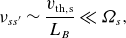 \begin{align} \nu _{ss^{\prime }} \sim \frac {v_{\mathrm{th, s}}}{L_{B}} & \ll \varOmega _s ,\end{align}
 \begin{align} \lambda _{\mathrm{mfp}} \sim L_{B} & \gg r_{\text{gyro},s}.\end{align}
Using a random walk estimate, we can calculate the classical heat transport coefficient in the perpendicular direction as $D_{\perp } \sim \nu _{ss^{\prime }} r_{\text{gyro},s}^2 \sim T^{-1/2}$
(Helander & Sigmar Reference Helander and Sigmar2005), whereas, using neoclassical theory, we have
$D_{\perp } \sim \nu _{ss^{\prime }} r_{\text{gyro},s}^2 \sim T^{-1/2}$
(Helander & Sigmar Reference Helander and Sigmar2005), whereas, using neoclassical theory, we have $\Delta r \sim r_{\text{gyro},s} \lvert {B}\rvert /\lvert {B}\rvert _{\text{poloidal}}$
with
$\Delta r \sim r_{\text{gyro},s} \lvert {B}\rvert /\lvert {B}\rvert _{\text{poloidal}}$
with $\lvert {B}\rvert$
and
$\lvert {B}\rvert$
and $\lvert {B}\rvert _{\text{poloidal}}$
given by the total and poloidal magnetic field strength, respectively. The transport coefficient is then
$\lvert {B}\rvert _{\text{poloidal}}$
given by the total and poloidal magnetic field strength, respectively. The transport coefficient is then $D_{\perp } \sim \nu _{ss^{\prime }} r_{\text{gyro},s}^2 \lvert {B}\rvert ^2/\lvert {B}\rvert _{\text{poloidal}}^2 \sim T^{-1/2} \lvert {B}\rvert ^2/\lvert {B}\rvert _{\text{poloidal}}^2$
. Note that the ratio
$D_{\perp } \sim \nu _{ss^{\prime }} r_{\text{gyro},s}^2 \lvert {B}\rvert ^2/\lvert {B}\rvert _{\text{poloidal}}^2 \sim T^{-1/2} \lvert {B}\rvert ^2/\lvert {B}\rvert _{\text{poloidal}}^2$
. Note that the ratio $\lvert {B}\rvert /\lvert {B}\rvert _{\text{poloidal}}$
strongly depends on the magnetic field geometry and significantly affects the regime of neoclassical transport.
$\lvert {B}\rvert /\lvert {B}\rvert _{\text{poloidal}}$
strongly depends on the magnetic field geometry and significantly affects the regime of neoclassical transport.
Magnetised plasmas can be weakly or strongly collisional as defined by the collisionality $\nu _{\star } = L_{B}/\lambda _{\mathrm{mfp}}$
. In a strongly collisional plasma, particles undergo frequent collisions without covering significant distances along a magnetic field line, i.e.
$\nu _{\star } = L_{B}/\lambda _{\mathrm{mfp}}$
. In a strongly collisional plasma, particles undergo frequent collisions without covering significant distances along a magnetic field line, i.e. $\nu _{\star } \gg 1$
. Conversely, in a weakly collisional plasma, particles can traverse a significant distance before colliding, i.e.
$\nu _{\star } \gg 1$
. Conversely, in a weakly collisional plasma, particles can traverse a significant distance before colliding, i.e. $\nu _{\star } \ll 1$
. Stellarator plasmas in practical applications tend to be weakly collisional.
$\nu _{\star } \ll 1$
. Stellarator plasmas in practical applications tend to be weakly collisional.
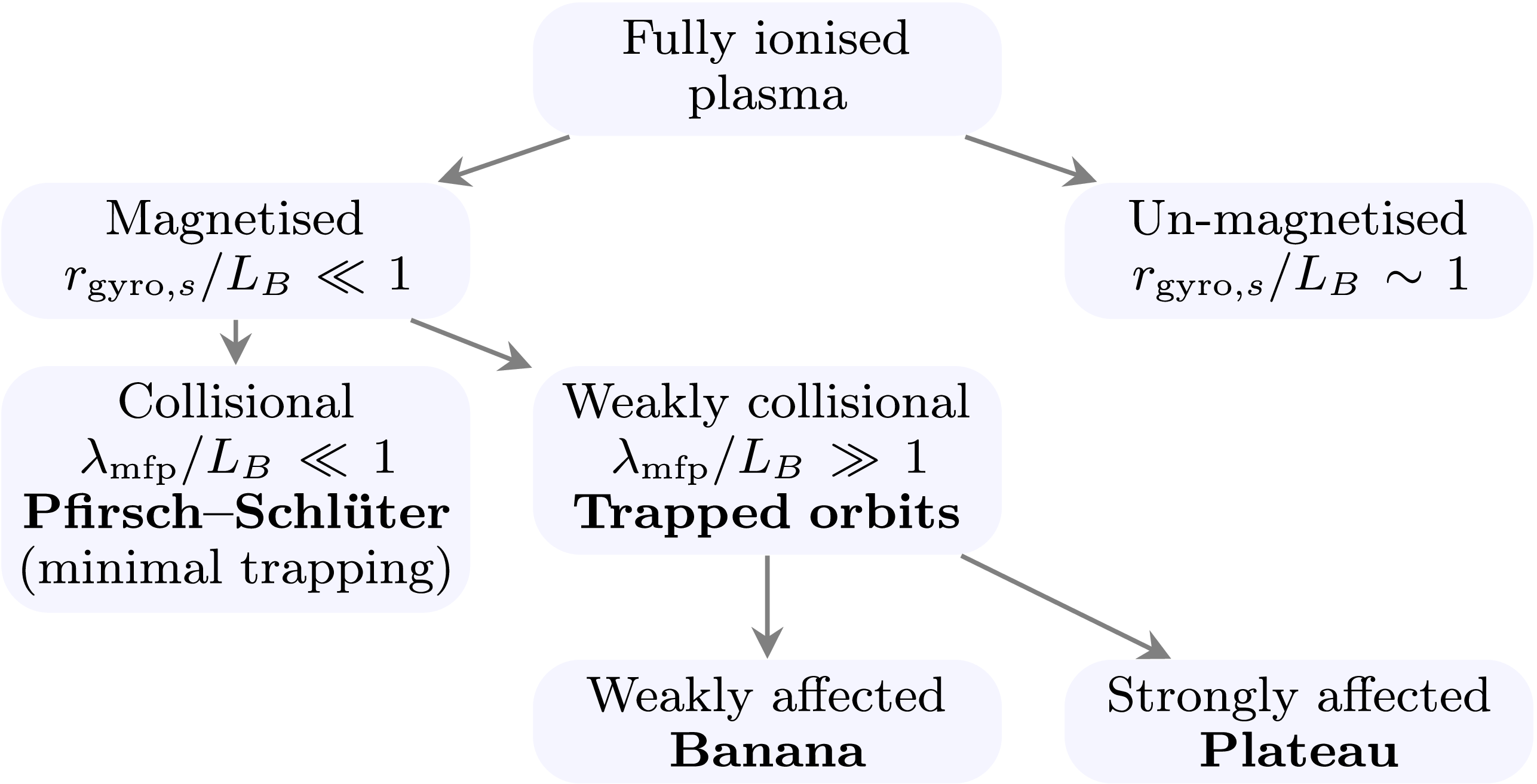
Based on the stellarator geometry, the weak collisionality regime can be further partitioned into the banana or plateau regime according to the reciprocal of the aspect ratio $\epsilon \sim \iota ^{-1} \lvert {B}\rvert _{\text{poloidal}} / \lvert {B}\rvert$
, where
$\epsilon \sim \iota ^{-1} \lvert {B}\rvert _{\text{poloidal}} / \lvert {B}\rvert$
, where $\iota$
is the rotational transform (Helander Reference Helander2014). Most stellarators lie in the regime where
$\iota$
is the rotational transform (Helander Reference Helander2014). Most stellarators lie in the regime where $\nu _{\star } \ll \epsilon ^{3/2}$
. This categorisation is illustrated in figure 1.
$\nu _{\star } \ll \epsilon ^{3/2}$
. This categorisation is illustrated in figure 1.
The standard neoclassical theory first enabled computation of the neoclassical transport coefficients in the low collisionality regime for a simplified model of the magnetic field. This analysis was later extended to stellarator magnetic fields (Kovrizhnykh Reference Kovrizhnykh1984; Ochs Reference Ochs2025). The following section outlines this process in one regime of interest to stellarator equilibrium optimisation.
A schematic categorising neoclassical transport.
2.1. Effective ripple
In the low collision limit $\nu _{\star } \ll \epsilon ^{3/2}$
, the neoclassical model studies the plasma distribution
$\nu _{\star } \ll \epsilon ^{3/2}$
, the neoclassical model studies the plasma distribution $f$
determined by a simplified Boltzmann equation known as the drift-kinetic equation. For a particle with mass
$f$
determined by a simplified Boltzmann equation known as the drift-kinetic equation. For a particle with mass $m$
, let
$m$
, let $\boldsymbol{v}_{\parallel }$
and
$\boldsymbol{v}_{\parallel }$
and $\boldsymbol{v}_{\perp }$
be the velocity parallel and orthogonal, respectively, to the unit vector magnetic field
$\boldsymbol{v}_{\perp }$
be the velocity parallel and orthogonal, respectively, to the unit vector magnetic field $\boldsymbol{b}$
. In the drift-kinetic equation, the velocity space may be parametrised with three independent coordinates: the total energy
$\boldsymbol{b}$
. In the drift-kinetic equation, the velocity space may be parametrised with three independent coordinates: the total energy $E$
, the magnetic moment
$E$
, the magnetic moment $\mu = m \lvert {v_{\perp }}\rvert ^{2}/(2 \lvert {B}\rvert )$
and the gyrophase angle. In this treatment, the equation is averaged over the gyrophase angle. We seek a steady-state solution and linearise the distribution of guiding centres
$\mu = m \lvert {v_{\perp }}\rvert ^{2}/(2 \lvert {B}\rvert )$
and the gyrophase angle. In this treatment, the equation is averaged over the gyrophase angle. We seek a steady-state solution and linearise the distribution of guiding centres $f = f_0 + f_1$
into a background
$f = f_0 + f_1$
into a background $f_0$
that is Maxwellian in velocity and a higher order correction
$f_0$
that is Maxwellian in velocity and a higher order correction $f_1$
. Thus, the background is parametrised in velocity space with
$f_1$
. Thus, the background is parametrised in velocity space with $E$
and the higher order correction with
$E$
and the higher order correction with $(E, \mu )$
. The linearised drift-kinetic equation reduces to the following partial differential equation (PDE) (Abel et al. Reference Abel, Plunk, Wang, Barnes, Cowley, Dorland and Schekochihin2013):
$(E, \mu )$
. The linearised drift-kinetic equation reduces to the following partial differential equation (PDE) (Abel et al. Reference Abel, Plunk, Wang, Barnes, Cowley, Dorland and Schekochihin2013):
 \begin{align}\mathcal{C}[f] = \boldsymbol{v}_{\mathrm{D}s} \boldsymbol{\cdot }\boldsymbol{\nabla } f_0 + \lvert {v_{\parallel }}\rvert \boldsymbol{b} \boldsymbol{\cdot }\boldsymbol{\nabla } f_1 ,\end{align}
 \begin{align}\boldsymbol{v}_{\mathrm{D}s} = \frac {\lvert {v_{\parallel }}\rvert ^2}{\varOmega _s} \boldsymbol{b} \times (\boldsymbol{b} \boldsymbol{\cdot }\boldsymbol{\nabla }\boldsymbol{b}) + \frac {\lvert {v_{\perp }}\rvert ^2}{2 \varOmega _s} \frac {\boldsymbol{b} \times \boldsymbol{\nabla } \lvert {B}\rvert }{\lvert {B}\rvert } + \boldsymbol{v}_{\mathrm{Ba}\tilde{\mathrm{n}}\mathrm{os}}.\end{align}
The electric field is neglected in this section as we focus on the $1/\nu$
collisionality regime.
$1/\nu$
collisionality regime.
To reduce neoclassical transport, one may minimise the radial particle flux density,
 \begin{equation} \varGamma = \int\!\mathrm{d}{^3\boldsymbol{v}} \; f_1 \boldsymbol{v}_{\mathrm{D}s}\boldsymbol{\cdot }\boldsymbol{\nabla } \psi .\end{equation}
Appendix B shows a derivation to extract a dimensionless quantity $\varGamma _0$
(2.8) for the optimisation objective which is proportional to the flux surface average
$\varGamma _0$
(2.8) for the optimisation objective which is proportional to the flux surface average $\langle \varGamma \rangle$
(B13).
$\langle \varGamma \rangle$
(B13).
 \begin{align} \langle \varGamma \rangle & = -\varGamma _0 \frac {2^{3/2} \mathrm{\pi } c^2}{3^2 e^2 m^{3/2}} \int _{0}^{\infty } \mathrm{d} E \; \frac {E^{5/2}}{\nu } \frac {\partial f_0}{\partial \psi }\\[-10pt]\nonumber \end{align}
 \begin{align} \varGamma _0 & = \left ({\int _{0}^{2\mathrm{\pi }} \mathrm{d} \alpha \int _{\lvert {B}\rvert _{\text{min}}}^{\lvert {B}\rvert _{\text{max}}} \frac {\mathrm{d} \varrho }{\varrho ^3} \; \sum _{w} \frac {I_1^2}{I_2} }\right ) \left ({\int _{0}^{2\mathrm{\pi }} \mathrm{d} \alpha \int _{\zeta _1}^{\zeta _2} \frac {\mathrm{d} \zeta }{\boldsymbol{B} \boldsymbol{\cdot }\boldsymbol{\nabla } \zeta }}\right )^{-1}\\[-10pt]\nonumber \end{align}
 \begin{align} I_1(\psi , \alpha , \varrho , w) & = \int _{\zeta _1(w)}^{\zeta _2(w)} \frac {\mathrm{d} \zeta }{\boldsymbol{B}\boldsymbol{\cdot }\boldsymbol{\nabla } \zeta } \left ({1 - \lvert {B}\rvert / \varrho }\right )^{1/2} \left ({4 \varrho / \lvert {B}\rvert - 1}\right ) \lvert {\boldsymbol{\nabla }\psi }\rvert \kappa _{\mathrm{G}} \\[-10pt]\nonumber\end{align}
 \begin{align} I_2(\psi , \alpha , \varrho , w) & = \int _{\zeta _1(w)}^{\zeta _2(w)} \frac {\mathrm{d} \zeta }{\boldsymbol{B}\boldsymbol{\cdot }\boldsymbol{\nabla } \zeta } \left ({1 - \lvert {B}\rvert / \varrho }\right )^{1/2}\\[6pt]\nonumber \end{align}
The quantity $\kappa _{\mathrm{G}}$
is the geodesic curvature of the field line (B5) and the velocity space coordinate
$\kappa _{\mathrm{G}}$
is the geodesic curvature of the field line (B5) and the velocity space coordinate $\varrho$
is defined as
$\varrho$
is defined as
 \begin{equation} \varrho = E / \mu . \end{equation}
The index $w$
labels the well with boundaries
$w$
labels the well with boundaries $\zeta _1(w)$
and
$\zeta _1(w)$
and $\zeta _2(w)$
where a bouncing particle is trapped. These boundaries are referred to as bounce points. Only the particles which are trapped within the interval
$\zeta _2(w)$
where a bouncing particle is trapped. These boundaries are referred to as bounce points. Only the particles which are trapped within the interval $[{\zeta _1, \zeta _2}]$
are considered so that
$[{\zeta _1, \zeta _2}]$
are considered so that $\zeta _1 \leqslant \min _w \zeta _1(w)$
and
$\zeta _1 \leqslant \min _w \zeta _1(w)$
and $\max _w \zeta _2(w) \leqslant \zeta _2$
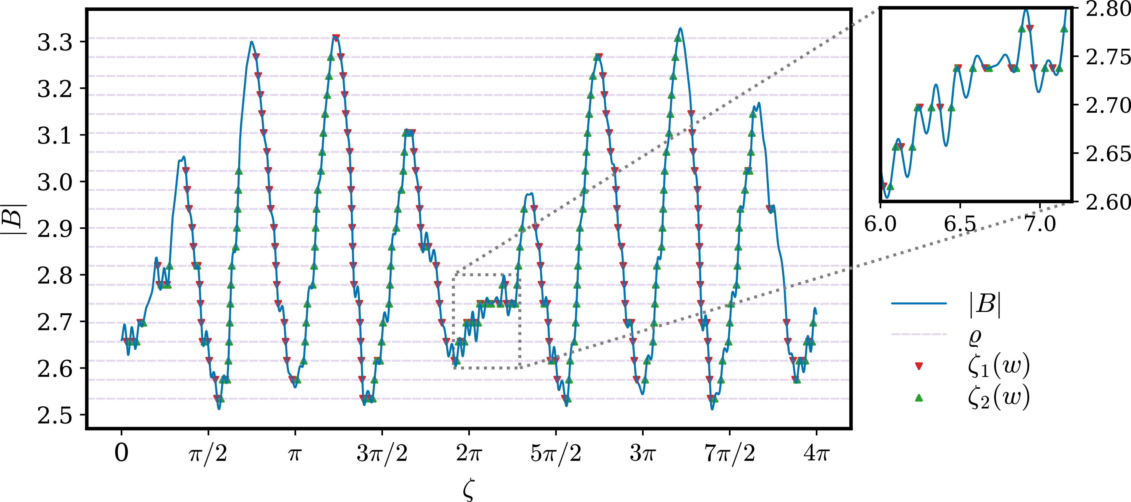
. An illustration is shown in figure 2.
$\max _w \zeta _2(w) \leqslant \zeta _2$
. An illustration is shown in figure 2.
In axisymmetric configurations, integration along the field line for a single poloidal transit between two global maxima of $\lvert {B}\rvert$
is sufficient for convergence of
$\lvert {B}\rvert$
is sufficient for convergence of $\varGamma _0$
. On irrational magnetic surfaces, it is sufficient to integrate along a single field line (D’haeseleer et al. Reference D’haeseleer, Hitchon, Callen and Shohet2012, § 4.9). On a rational or near-rational surface in non-axisymmetric configurations, it is necessary to integrate along multiple field lines until the surface is covered sufficiently.
$\varGamma _0$
. On irrational magnetic surfaces, it is sufficient to integrate along a single field line (D’haeseleer et al. Reference D’haeseleer, Hitchon, Callen and Shohet2012, § 4.9). On a rational or near-rational surface in non-axisymmetric configurations, it is necessary to integrate along multiple field lines until the surface is covered sufficiently.
The effective ripple modulation amplitude $\epsilon _{\text{eff}}$
is related to
$\epsilon _{\text{eff}}$
is related to $\varGamma _0$
as follows:
$\varGamma _0$
as follows:
 \begin{equation} \epsilon _{\text{eff}}^{3/2} = \frac {\mathrm{\pi }}{2^{7/2}}\frac {(B_0 R_0)^2}{\langle \lvert {\boldsymbol{\nabla } \psi }\rvert \rangle ^{2}} \varGamma _0, \end{equation}
where $B_0$
is a background magnetic field typically chosen to be
$B_0$
is a background magnetic field typically chosen to be $\lvert {B}\rvert _{\text{max}}$
and
$\lvert {B}\rvert _{\text{max}}$
and $R_0$
is the average major radius of the stellarator. A reason
$R_0$
is the average major radius of the stellarator. A reason $\epsilon _{\text{eff}}$
is preferred to
$\epsilon _{\text{eff}}$
is preferred to $\varGamma _0$
as an optimisation objective is that the latter vanishes near the magnetic axis, which reduces the ability to distinguish between good and bad configurations. Since
$\varGamma _0$
as an optimisation objective is that the latter vanishes near the magnetic axis, which reduces the ability to distinguish between good and bad configurations. Since $\epsilon _{\text{eff}}$
depends only on geometry, reducing it by varying the plasma boundary can reduce the radial neoclassical loss of trapped particles.
$\epsilon _{\text{eff}}$
depends only on geometry, reducing it by varying the plasma boundary can reduce the radial neoclassical loss of trapped particles.
Bounce points within $(\zeta _1, \zeta _2) = (0, 4 \mathrm{\pi })$
on the field line
$(\zeta _1, \zeta _2) = (0, 4 \mathrm{\pi })$
on the field line $(\psi , \alpha ) = (\psi_{\text{plasma boundary}}, 0)$
for a mesh of
$(\psi , \alpha ) = (\psi_{\text{plasma boundary}}, 0)$
for a mesh of $\varrho$
values on a W7-X stellarator. For a given
$\varrho$
values on a W7-X stellarator. For a given $\varrho$
marked by a horizontal line,
$\varrho$
marked by a horizontal line, $\lvert {v_{\parallel }}\rvert = 0$
at the bounce points marked by triangles. The plasma distribution vanishes in the hypograph of
$\lvert {v_{\parallel }}\rvert = 0$
at the bounce points marked by triangles. The plasma distribution vanishes in the hypograph of $\lvert {B}\rvert$
.
$\lvert {B}\rvert$
.
3. Algorithm
We briefly describe a few fundamental parts of our algorithm. Section 1 discusses the bounce integral in more detail. In § 2, we describe efficient quadrature used for these integrals. Section 3 discusses our inverse method to solve the ideal MHD equation. In §§ 4–6, we describe our approach to obtain data along field lines.
To motivate the need for an efficient algorithm, let us estimate the computational cost of bounce-averaging with a blunt approach to the computation. After discretising to $N_s$
field lines, where each field line is followed over
$N_s$
field lines, where each field line is followed over $N_w$
magnetic wells for each of
$N_w$
magnetic wells for each of $N_{\varrho }$
pitch angles, there will be
$N_{\varrho }$
pitch angles, there will be $\mathcal{O}(N_s N_w N_{\varrho })$
bounce integrals. With
$\mathcal{O}(N_s N_w N_{\varrho })$
bounce integrals. With $N_{q}$
quadrature points each, the integrand is evaluated at
$N_{q}$
quadrature points each, the integrand is evaluated at $\mathcal{O}(N_s N_w N_{\varrho } N_q) \sim 10^{8}$
points. Furthermore, the path of integration is unknown a priori because the field lines move during optimisation. Finding the position of the field lines on a known grid may involve
$\mathcal{O}(N_s N_w N_{\varrho } N_q) \sim 10^{8}$
points. Furthermore, the path of integration is unknown a priori because the field lines move during optimisation. Finding the position of the field lines on a known grid may involve $N_i$
Newton iterations for each point. With
$N_i$
Newton iterations for each point. With $N_c$
spectral coefficients used to approximate the map on which that root-finding is done, the cost grows to
$N_c$
spectral coefficients used to approximate the map on which that root-finding is done, the cost grows to $\mathcal{O}(N_c N_i N_s N_w N_{\varrho } N_q)$
. Moreover, the memory required to reverse-mode differentiate the objective grows linearly with the problem size.
$\mathcal{O}(N_c N_i N_s N_w N_{\varrho } N_q)$
. Moreover, the memory required to reverse-mode differentiate the objective grows linearly with the problem size.
3.1. Bounce integral
The bounce integral of $x$
may be written as a time-weighted integral over the trajectory of the particle along its bounce orbit (Mackenbach et al. Reference Mackenbach, Duff, Gerard, Proll, Helander and Hegna2023b
, § 2). Since the dynamics parallel to the field lines dominate, the particle trajectory may be approximated to follow field lines by parametrising time
$x$
may be written as a time-weighted integral over the trajectory of the particle along its bounce orbit (Mackenbach et al. Reference Mackenbach, Duff, Gerard, Proll, Helander and Hegna2023b
, § 2). Since the dynamics parallel to the field lines dominate, the particle trajectory may be approximated to follow field lines by parametrising time $t$
as the distance along a field-line following coordinate. Since the magnetic moment is an adiabatic invariant for which the gyro-average of
$t$
as the distance along a field-line following coordinate. Since the magnetic moment is an adiabatic invariant for which the gyro-average of $\mathrm{d} \mu / \mathrm{d} t$
is approximately zero, the pitch angle of a bouncing particle stays nearly constant over the time scale to complete bounce orbits when energy is conserved. Labelling the boundaries
$\mathrm{d} \mu / \mathrm{d} t$
is approximately zero, the pitch angle of a bouncing particle stays nearly constant over the time scale to complete bounce orbits when energy is conserved. Labelling the boundaries $\zeta _1(w)$
and
$\zeta _1(w)$
and $\zeta _2(w)$
of magnetic well
$\zeta _2(w)$
of magnetic well $w$
where the parallel velocity vanishes, using the streamline property in curvilinear coordinates,
$w$
where the parallel velocity vanishes, using the streamline property in curvilinear coordinates,
 \begin{equation} \lvert {v_{\parallel }}\rvert \mathrm{d} t = \frac {\mathrm{d} \zeta }{\boldsymbol{b} \boldsymbol{\cdot }\boldsymbol{\nabla } \zeta }, \end{equation}
and $\lvert {v_{\parallel }}\rvert ^2 = (2 E / m) (1 - \lvert {B}\rvert / \varrho )$
, then allows writing the integral as follows:
$\lvert {v_{\parallel }}\rvert ^2 = (2 E / m) (1 - \lvert {B}\rvert / \varrho )$
, then allows writing the integral as follows:
 \begin{equation} \overline {x}(\psi , \alpha , \varrho , w) = \frac {m^{1/2}}{(2 E)^{1/2}} \int _{\zeta _{1}(w)}^{\zeta _{2}(w)} \frac {\mathrm{d} \zeta }{\boldsymbol{b}\boldsymbol{\cdot }\boldsymbol{\nabla } \zeta } (1 - \lvert {B}\rvert / \varrho )^{-1/2} x. \end{equation}
More generally, integrals between bounce points involve a map $g$
, smooth in
$g$
, smooth in $\zeta$
, weighted by a map with behaviour matching
$\zeta$
, weighted by a map with behaviour matching $\lvert {v_{\parallel }}\rvert ^{\eta }$
near the bounce points,
$\lvert {v_{\parallel }}\rvert ^{\eta }$
near the bounce points,
 \begin{equation} \int _{\zeta _{1}(w)}^{\zeta _{2}(w)} \mathrm{d} \zeta \, \lvert {v_{\parallel }}\rvert ^{\eta } g(\psi , \alpha , \zeta , \varrho ), \quad \eta \in \left \{ -1, 1 \right \}\!. \end{equation}
3.2. Quadrature
Gaussian quadrature approximates $\int _{-1}^{1} \mathrm{d} \zeta \, \varsigma g(\zeta ) \approx \sum _{i=1}^{N_q} \sigma _i g(\zeta _i)$
for some weight
$\int _{-1}^{1} \mathrm{d} \zeta \, \varsigma g(\zeta ) \approx \sum _{i=1}^{N_q} \sigma _i g(\zeta _i)$
for some weight $\varsigma$
positive and continuous in the interior by approximating
$\varsigma$
positive and continuous in the interior by approximating $g$
with its Hermite interpolation polynomial and choosing
$g$
with its Hermite interpolation polynomial and choosing $\sigma _i, \zeta _i$
to avoid evaluating the derivative (Süli & Mayers Reference Süli and Mayers2003). For integrable (3.3), we can construct such a quadrature for
$\sigma _i, \zeta _i$
to avoid evaluating the derivative (Süli & Mayers Reference Süli and Mayers2003). For integrable (3.3), we can construct such a quadrature for $\varsigma$
matching the non-polynomial behaviour of
$\varsigma$
matching the non-polynomial behaviour of $\lvert {v_{\parallel }}\rvert ^{\eta }$
or, more generally, employ a change of variable whose Jacobian vanishes slowly near singularities such that the integrand can then be approximated by a low-degree polynomial. In the latter approach, the transformation should also be mild enough to prevent unnecessary clustering of quadrature points that would increase the condition number of the problem.
$\lvert {v_{\parallel }}\rvert ^{\eta }$
or, more generally, employ a change of variable whose Jacobian vanishes slowly near singularities such that the integrand can then be approximated by a low-degree polynomial. In the latter approach, the transformation should also be mild enough to prevent unnecessary clustering of quadrature points that would increase the condition number of the problem.
Our transformation for bounce integrals defines $z$
such that
$z$
such that $a_1(w, a_2[z]) = \zeta$
,
$a_1(w, a_2[z]) = \zeta$
,
 \begin{align} a_1 & \colon \begin{cases} \mathbb{N} \times \left [{-1, 1}\right ] \to \mathbb{R}, \\ w, z \mapsto (z + 1) [\zeta _{2}(w) - \zeta _{1}(w)]/2 + \zeta _{1}(w), \end{cases}\\[-12pt]\nonumber \end{align}
 \begin{align} a_2 & \colon \begin{cases} \left [{-1, 1}\right ] \to \left [{-1, 1}\right ]\!, \\ z \mapsto \sin (\mathrm{\pi } z / 2), \end{cases}\\[-12pt]\nonumber \end{align}
 \begin{align} \int _{\zeta _{1}(w)}^{\zeta _{2}(w)} \mathrm{d} \zeta \, \lvert {v_{\parallel }}\rvert ^{\eta } g(\zeta ) & \approx \frac {\zeta _{2}(w) - \zeta _{1}(w)}{2} \sum _{i=1}^{N_q} \sigma _i \lvert {v_{\parallel }}\rvert ^{\eta } g(a_1(w, a_2[z_i])) .\end{align}
When neither bounce point is on a local maximum of the potential, the midpoint scheme in $z$
(3.7) is exponentially accurate,Footnote
1
$z$
(3.7) is exponentially accurate,Footnote
1
 \begin{equation} \sigma _i = \mathrm{\pi } \sin \left [{\mathrm{\pi } (2 i - 1) / (2 N_q)}\right ] / N_q, \quad a_2[z_i] = \cos \left [{\mathrm{\pi } (2i - 1) /(2 N_q)}\right ] .\end{equation}
If, in addition, $\eta = 1$
, then (3.8) yields faster convergence,
$\eta = 1$
, then (3.8) yields faster convergence,
 \begin{equation} \sigma _i = \mathrm{\pi } \sin \left [{\mathrm{\pi } i /(N_q + 1)}\right ] / (N_q + 1), \quad a_2[z_i] = \cos \left [{\mathrm{\pi } i /(N_q + 1)}\right ]. \end{equation}
In general, Gauss–Legendre quadrature in $z$
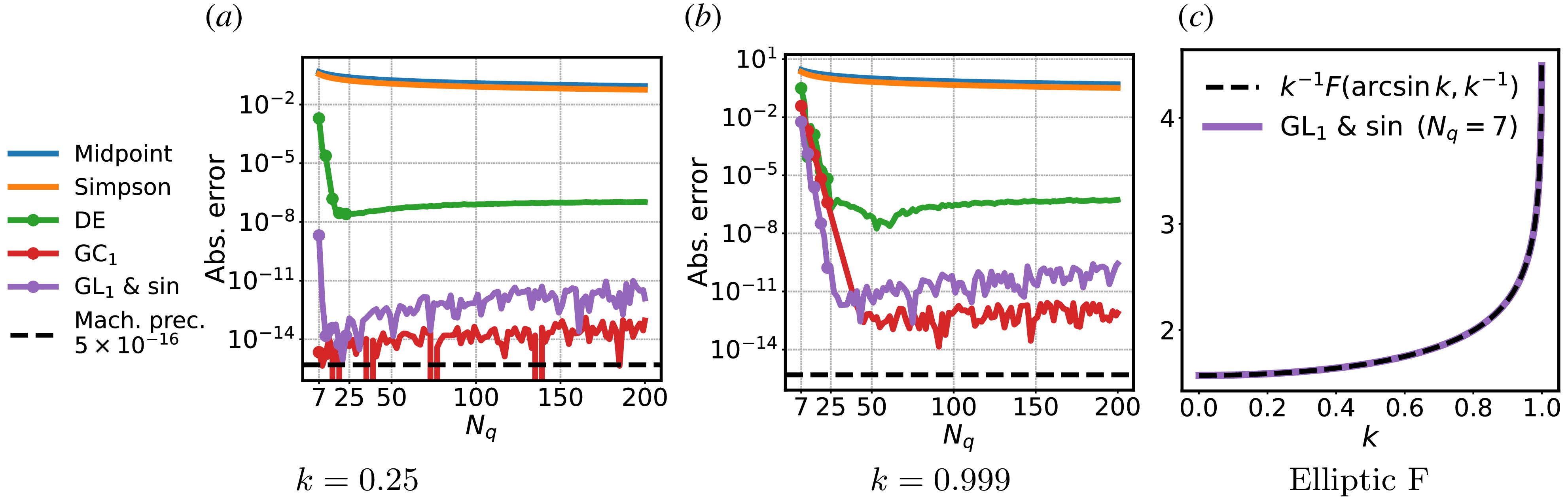
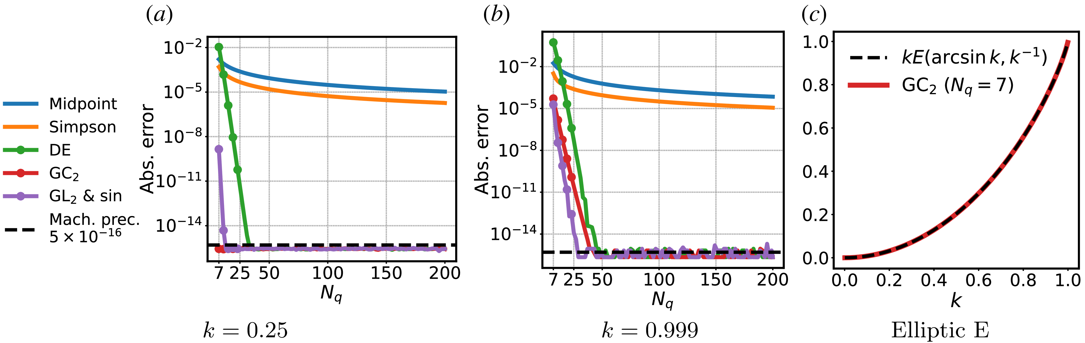
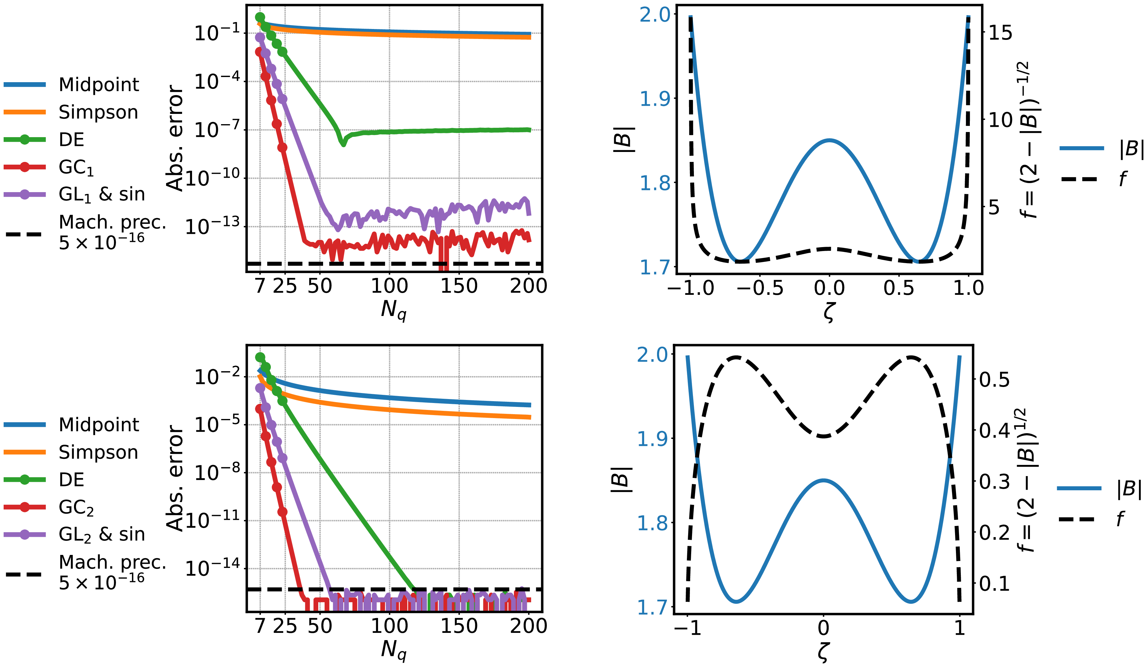
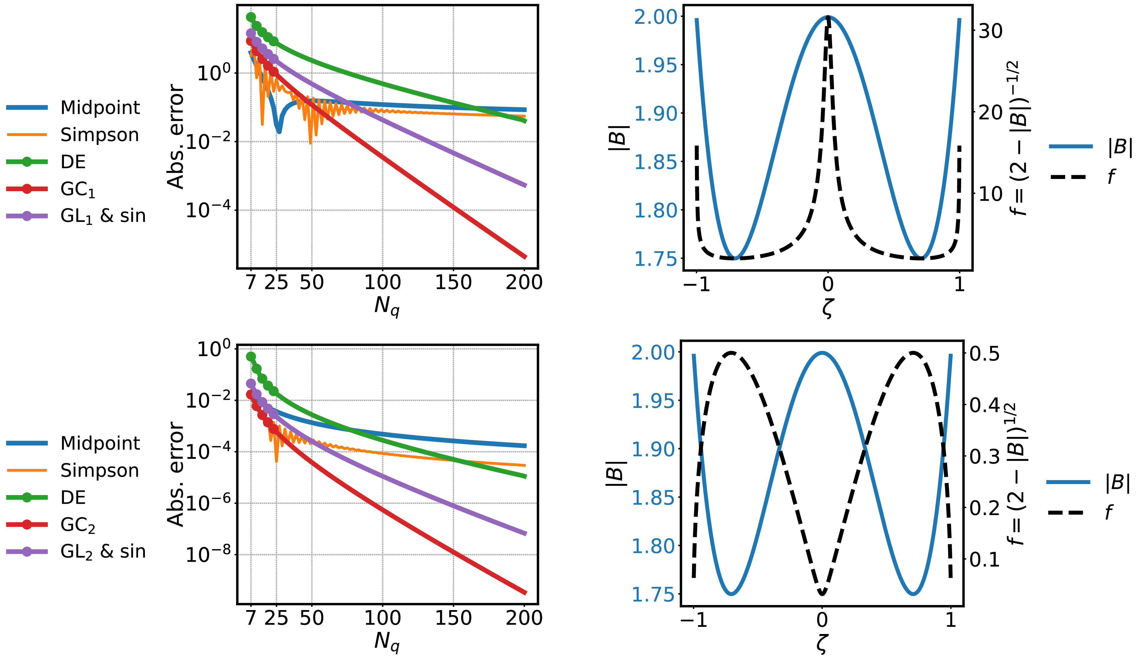
is exponentially accurate if (3.3) is integrable. Figures 3, 4, 5 and 6 illustrate the convergence.
$z$
is exponentially accurate if (3.3) is integrable. Figures 3, 4, 5 and 6 illustrate the convergence.
It is often of interest to integrate a nonlinear combination of bounce integrals over $\varrho$
. Such integrands can be non-smooth in
$\varrho$
. Such integrands can be non-smooth in $\varrho$
due to the logarithmic divergence (Calvo et al. Reference Calvo, Parra, Velasco and Alonso2017, § 4) of (3.2) as
$\varrho$
due to the logarithmic divergence (Calvo et al. Reference Calvo, Parra, Velasco and Alonso2017, § 4) of (3.2) as $\varrho$
approaches the value of
$\varrho$
approaches the value of $\lvert {B}\rvert$
at any local maxima within or at the bounce points. The Alpert (Reference Alpert1999) quadratures are high-order accurate for these singularities.
$\lvert {B}\rvert$
at any local maxima within or at the bounce points. The Alpert (Reference Alpert1999) quadratures are high-order accurate for these singularities.
We compare the following quadratures in their ability to compute elliptic integrals (3.9), (3.10), which are similar to bounce integrals in a simple stellarator geometry.
-
(i) Midpoint scheme.
-
(ii) Simpson’s 1/3 in the interior completed by a midpoint scheme.
-
(iii) Double exponential (DE) $\tanh -\sinh$
.
$\tanh -\sinh$
. -
(iv) Implicitly weighted Gauss–Chebyshev of the first (
$\mathrm{GC}_1$
) (3.7) or second kind (
$\mathrm{GC}_2$
) (3.8). -
(v) Gauss–Legendre (
$\mathrm{GL}_1$
) or Gauss–Lobatto–Legendre (
$\mathrm{GL}_2$
) each composed with the
$\sin$
transformation in (3.5). Compared with item (iv), this quadrature offers more resolution near the boundary and less in the interior.


 \begin{align} \int _{-\arcsin k}^{\arcsin k} \mathrm{d} \zeta \, (k^2 - \sin ^2 \zeta )^{-1/2} & \underset {(\mathrm{C11})}{=} 2 K(k)\end{align}
 \begin{align} \int _{-\arcsin k}^{\arcsin k} \mathrm{d} \zeta \, (k^2 - \sin ^2 \zeta )^{1/2} & \underset {(\mathrm{C12})}{=} 2 E(k) + 2 (k^2-1) K(k)\end{align}
To further benchmark the quadratures in a magnetic field with ripples, we show two more cases that model particles trapped in the following wells in figures 5 and 6.
Convergence of quadratures for (3.9). $\mathrm{GC}_1$
and
$\mathrm{GC}_1$
and $\mathrm{GL}_1$
show spectral convergence whereas midpoint, Simpson and double exponential quadratures hit floating point plateaus early.
$\mathrm{GL}_1$
show spectral convergence whereas midpoint, Simpson and double exponential quadratures hit floating point plateaus early.
Convergence of quadratures for (3.10). $\mathrm{GC}_2$
and
$\mathrm{GC}_2$
and $\mathrm{GL}_2$
show spectral convergence.
$\mathrm{GL}_2$
show spectral convergence.
3.3. Inverse method
In this section, we briefly discuss how we find stellarator equilibria. At static equilibrium, the ideal MHD equations that approximate the behaviour of the plasma reduce to
 \begin{align} \boldsymbol{B} \boldsymbol{\cdot }\boldsymbol{\nabla } \boldsymbol{B} & = \boldsymbol{\nabla } \left ({p + \lvert {B}\rvert ^2 / 2}\right )\!,\end{align}
 \begin{align} \boldsymbol{\nabla } \boldsymbol{\cdot }\boldsymbol{B} & = 0,\end{align}
which describes a balance between the plasma pressure $p$
, magnetic field pressure
$p$
, magnetic field pressure $\lvert {B}\rvert ^2$
and the effect of field line curvature
$\lvert {B}\rvert ^2$
and the effect of field line curvature $\boldsymbol{B}\boldsymbol{\cdot }\boldsymbol{\nabla } \boldsymbol{B}$
. We solve the ideal MHD equation using an inverse method. The computational domain is a solid torus in curvilinear flux coordinates
$\boldsymbol{B}\boldsymbol{\cdot }\boldsymbol{\nabla } \boldsymbol{B}$
. We solve the ideal MHD equation using an inverse method. The computational domain is a solid torus in curvilinear flux coordinates $(\rho , \theta , \zeta )$
, where
$(\rho , \theta , \zeta )$
, where $\rho = (\psi /\psi _{\text{plasma boundary}})^{1/2}$
and
$\rho = (\psi /\psi _{\text{plasma boundary}})^{1/2}$
and $(\theta , \zeta )$
are angles on a doubly-periodic surface. Here,
$(\theta , \zeta )$
are angles on a doubly-periodic surface. Here, $\varLambda$
and
$\varLambda$
and $\omega$
are to be determined maps that relate the angles
$\omega$
are to be determined maps that relate the angles $(\theta , \zeta )$
that parametrise a given plasma boundary to the Clebsch angle,
$(\theta , \zeta )$
that parametrise a given plasma boundary to the Clebsch angle,
Convergence of quadratures for the quantity labeled by $f$
.
$f$
.
Convergence of quadratures for the quantity labelled by $f$
. In the top row, the integrand becomes nearly non-integrable as the parallel velocity nearly vanishes at
$f$
. In the top row, the integrand becomes nearly non-integrable as the parallel velocity nearly vanishes at $\zeta = 0$
. In either case, splitting the quadrature there recovers fast convergence.
$\zeta = 0$
. In either case, splitting the quadrature there recovers fast convergence.
 \begin{equation} \alpha = \theta + \varLambda - \iota (\zeta + \omega ). \end{equation}
Fourier–Zernike series parametrised in flux coordinates $(\rho , \theta , \zeta )$
are chosen to approximate
$(\rho , \theta , \zeta )$
are chosen to approximate $\varLambda$
,
$\varLambda$
, $\omega$
and the map to a cylindrical coordinate system
$\omega$
and the map to a cylindrical coordinate system $(R, \phi , Z)$
in the lab frame,
$(R, \phi , Z)$
in the lab frame,
 \begin{equation} R(\rho , \theta , \zeta ) \boldsymbol{\hat {R}}(\phi ) + Z(\rho , \theta , \zeta ) \boldsymbol{\hat {Z}}. \end{equation}
It can be shown from (2.1) that $\boldsymbol{\nabla } \theta \times \boldsymbol{\nabla } \zeta \neq \boldsymbol{0}$
implies
$\boldsymbol{\nabla } \theta \times \boldsymbol{\nabla } \zeta \neq \boldsymbol{0}$
implies
 \begin{align}\boldsymbol{B} \boldsymbol{\cdot }\boldsymbol{\nabla } \theta & = -[\boldsymbol{\nabla } \psi \boldsymbol{\cdot }(\boldsymbol{\nabla } \theta \times \boldsymbol{\nabla } \zeta )] \left ({\frac {\partial {\alpha }}{\partial {\zeta }}}\right )_{\psi , \theta },\end{align}
 \begin{align} \boldsymbol{B} \boldsymbol{\cdot }\boldsymbol{\nabla } \zeta & = + [\boldsymbol{\nabla } \psi \boldsymbol{\cdot }(\boldsymbol{\nabla } \theta \times \boldsymbol{\nabla } \zeta )] \left ({\frac {\partial {\alpha }}{\partial {\theta }}}\right )_{\psi , \zeta } .\end{align}
Thus, we find equilibria by searching for a combination $(R, Z, \varLambda , \omega )$
to reduce the force balance error (3.11) at a set of collocation points using pseudo-spectral methods, subject to constraints on the pressure profile and the rotational transform or toroidal current profile. This boundary value problem is then solved as a minimisation problem using a trust-region method. In an optimisation constrained by force balance, varying
$(R, Z, \varLambda , \omega )$
to reduce the force balance error (3.11) at a set of collocation points using pseudo-spectral methods, subject to constraints on the pressure profile and the rotational transform or toroidal current profile. This boundary value problem is then solved as a minimisation problem using a trust-region method. In an optimisation constrained by force balance, varying $(R, Z, \varLambda , \omega )$
changes the magnetic field and (3.14) such that (3.13) remains valid.
$(R, Z, \varLambda , \omega )$
changes the magnetic field and (3.14) such that (3.13) remains valid.
Two advantages of this inverse approach for optimisation with bounce-averaged objectives are stated as follows.
-
(i) The variables
$(\theta , \zeta )$
on the boundary surface may be constructed so that maps parametrised in these coordinates are spectrally condensed (Hirshman & Breslau Reference Hirshman and Breslau1998; Hindenlang, Plunk & Maj Reference Hindenlang, Plunk and Maj2025). Consequently, maps parametrised in
$(\rho , \theta , \zeta )$
in the plasma volume tend to have spectral expansions that converge more rapidly. -
(ii) Force balance and other geometric objectives are best computed on a particular grid in
$(\rho , \theta , \zeta )$
, which is fixed throughout optimisation. This ensures the spectral basis for
$(R, Z, \varLambda , \omega )$
can be precomputed, avoiding ‘off-grid’ interpolation of a three-dimensional basis that bottlenecks pseudo-spectral codes (Boyd Reference Boyd2013, § 10.7). Furthermore, if the coordinate system varied throughout the optimisation, then so does the optimal grid for interpolation and quadrature. To preserve spectral accuracy, a pseudo-spectral code must first find this optimal grid and compute the basis there. This ‘moving-grid’ interpolation is doubly expensive in optimisation because the mentioned tasks must also be differentiated, which consumes significant memory.


These qualities enable faster generation of magnetic field data, which we discuss in the following section.
3.4. Fast interpolation
In this section, we outline our method for fast interpolation.
The Zernike basis concentrates the frequency transform of smooth maps on discs at lower frequencies than geometry-agnostic tensor-product bases. Boyd & Yu (Reference Boyd and Yu2011) show the required number of spectral coefficients is typically half that of Fourier–Chebyshev. This ensures an optimisation that varies a finite number of coefficients in the Fourier–Zernike series for $(R, Z, \varLambda , \omega )$
at a time has more freedom compared with expansions in other bases. However, the Zernike basis is expensive to evaluate.
$(R, Z, \varLambda , \omega )$
at a time has more freedom compared with expansions in other bases. However, the Zernike basis is expensive to evaluate.
Our algorithm computes the Fourier–Zernike basis once prior to optimisation on a uniform $K_{\theta } \times K_{\zeta }$
grid in
$K_{\theta } \times K_{\zeta }$
grid in $(\theta , N_{\text{FP}} \zeta ) \in [{0, 2 \mathrm{\pi }})^2$
on each surface. Any smooth, periodic map
$(\theta , N_{\text{FP}} \zeta ) \in [{0, 2 \mathrm{\pi }})^2$
on each surface. Any smooth, periodic map $g$
required by the objective is computed from
$g$
required by the objective is computed from $(R, Z, \varLambda , \omega )$
on this grid and interpolated with a fast Fourier transform (FFT). The resulting Fourier series are evaluated using type-2 non-uniform FFTs with computational cost that is linearithmic in
$(R, Z, \varLambda , \omega )$
on this grid and interpolated with a fast Fourier transform (FFT). The resulting Fourier series are evaluated using type-2 non-uniform FFTs with computational cost that is linearithmic in $K_{\theta } K_{\zeta }$
plus linear in the number of points to evaluate (Barnett et al. Reference Barnett, Magland and af Klinteberg2019; Barnett Reference Barnett2021; Hsuan Shih et al. Reference Satake, Okamoto and Sugama2021),
$K_{\theta } K_{\zeta }$
plus linear in the number of points to evaluate (Barnett et al. Reference Barnett, Magland and af Klinteberg2019; Barnett Reference Barnett2021; Hsuan Shih et al. Reference Satake, Okamoto and Sugama2021),
 \begin{align} g_{k_{\theta } k_{\zeta }} & = \frac {c_{k_{\theta }}}{4 \mathrm{\pi }^2} \iint _{[{0, 2\mathrm{\pi }})^2} \mathrm{d} \theta \, \mathrm{d} (N_{\text{FP}} \zeta ) \; g(\theta , N_{\text{FP}} \zeta ) \mathrm{e}^{-\mathrm{i} k_{\theta } \theta } \mathrm{e}^{-\mathrm{i} k_{\zeta } N_{\text{FP}} \zeta },\\[-10pt]\nonumber \end{align}
 \begin{align} g(\alpha , \zeta ) & = \sum _{k_{\theta }=0}^{\lfloor {K_{\theta }/2}\rfloor } \sum _{k_{\zeta }=-\lfloor {K_{\zeta } /2}\rfloor }^{\lceil {K_{\zeta }/2}\rceil - 1} \text{Real} \left ({g_{k_{\theta } k_{\zeta }} \mathrm{e}^{\mathrm{i} k_{\theta } \theta (\alpha , \zeta )} \mathrm{e}^{\mathrm{i} k_{\zeta } N_{\text{FP}} \zeta }}\right ), \\ c_{k_{\theta }} & = 1 \quad \text{ if } k_{\theta } \in \left \{ 0, K_{\theta }/2 \right \}; \text{ else } 2. \nonumber \end{align}
3.5. Map to the mesh of field lines
Evaluating maps along field lines requires finding the position of the field lines on some grid. To identify the coordinate $\theta$
at a given point
$\theta$
at a given point $(\alpha , \zeta )$
one may solve (3.13). To avoid repeating that inversion everywhere our objective demands, we compute the spectral projection
$(\alpha , \zeta )$
one may solve (3.13). To avoid repeating that inversion everywhere our objective demands, we compute the spectral projection $\{ a_{xy} \}$
of the map
$\{ a_{xy} \}$
of the map $\alpha , \zeta \mapsto \theta - \alpha$
onto a tensor-product basis
$\alpha , \zeta \mapsto \theta - \alpha$
onto a tensor-product basis $\{ b_{x y} \}$
that is orthogonal with respect to some weight
$\{ b_{x y} \}$
that is orthogonal with respect to some weight $\varsigma$
,
$\varsigma$
,
 \begin{equation} a_{x y} \sim \iint \mathrm{d} \alpha \, \mathrm{d} \zeta \; (\theta - \alpha ) \, \varsigma b^{*}_{x y}(\alpha , \zeta ) .\end{equation}
The Fourier–Chebyshev basis defined on the field period $(\alpha , N_{\text{FP}} \zeta ) \in [{0, 2 \mathrm{\pi }})^2$
is chosen for reasons discussed by Mason & Handscomb (Reference Mason and Handscomb2002, §§ 5.5, 5.6, 6.3.4) and Boyd (Reference Boyd2013, § 4.5),
$(\alpha , N_{\text{FP}} \zeta ) \in [{0, 2 \mathrm{\pi }})^2$
is chosen for reasons discussed by Mason & Handscomb (Reference Mason and Handscomb2002, §§ 5.5, 5.6, 6.3.4) and Boyd (Reference Boyd2013, § 4.5),
 \begin{equation} b_{xy}(\alpha , \zeta ) = \mathrm{e}^{\mathrm{i} x \alpha } \cos (y \arccos [N_{\text{FP}} \zeta / \mathrm{\pi } - 1]) .\end{equation}
On each flux surface, (3.13) is solved on a tensor-product grid of size $X \times Y$
on the Fourier nodes across field lines and the Chebyshev nodes along field lines using Newton iteration with a backtracking line search. The series (3.19) is computed by interpolating
$X \times Y$
on the Fourier nodes across field lines and the Chebyshev nodes along field lines using Newton iteration with a backtracking line search. The series (3.19) is computed by interpolating $\theta {-} \alpha$
on that grid with a discrete cosine transform along field lines, followed by an FFT across field lines. The convergence of the series is illustrated in figure 7.
$\theta {-} \alpha$
on that grid with a discrete cosine transform along field lines, followed by an FFT across field lines. The convergence of the series is illustrated in figure 7.
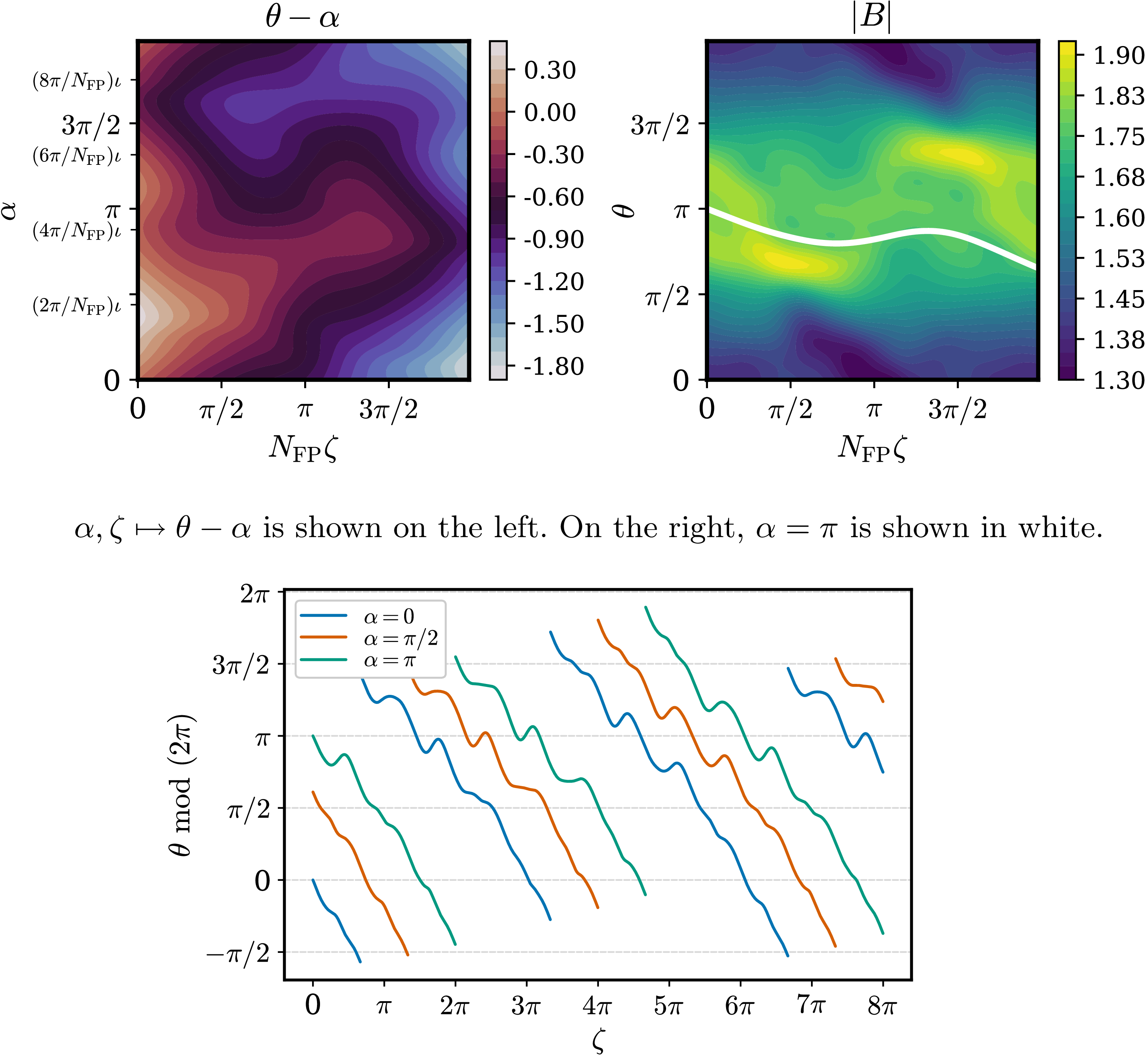
To extend the map beyond a single field period, we use
 \begin{align} \theta & \equiv \alpha _{\text{mod}} + \sum _{x=0}^{\lfloor {X/2}\rfloor } \sum _{y=0}^{Y - 1} \text{Real} \left ({a_{xy} b_{xy}(\alpha _{\text{mod}}, \zeta _{\text{mod}})}\right ) \pmod {2\mathrm{\pi }}, \\ \alpha _{\text{mod}} & = \alpha _{\text{shift}} \bmod (2 \mathrm{\pi }), \nonumber \\ \alpha _{\text{shift}} & = \alpha + \iota \lfloor {N_{\text{FP}} \zeta / (2 \mathrm{\pi })}\rfloor 2 \mathrm{\pi } /N_{\text{FP}}, \nonumber \\ \zeta _{\text{mod}} & = \zeta \bmod (2 \mathrm{\pi } / N_{\text{FP}}). \nonumber \end{align}
The equivalence (3.21) is due to $\alpha + \iota \zeta = \alpha _{\text{shift}} + \iota \zeta _{\text{mod}}$
and uniqueness of solutions to (3.13). Figure 8 shows an illustration. The construction and evaluation of this series is accelerated with partial summation (Boyd Reference Boyd2013, § 10).
$\alpha + \iota \zeta = \alpha _{\text{shift}} + \iota \zeta _{\text{mod}}$
and uniqueness of solutions to (3.13). Figure 8 shows an illustration. The construction and evaluation of this series is accelerated with partial summation (Boyd Reference Boyd2013, § 10).
Convergence of the spectral projection of $\alpha , \zeta \mapsto \theta - \alpha$
onto the Fourier–Chebyshev basis (3.21). Equation (3.13) was solved to error
$\alpha , \zeta \mapsto \theta - \alpha$
onto the Fourier–Chebyshev basis (3.21). Equation (3.13) was solved to error $\leqslant 10^{-7}$
. Note that if
$\leqslant 10^{-7}$
. Note that if $\omega \to \varLambda / \iota$
, then
$\omega \to \varLambda / \iota$
, then $\theta - \alpha \to \iota \zeta$
, so the spectral width reduces to one parameter. Thus, if the optimiser is motivated to match higher frequency spectral coefficients of
$\theta - \alpha \to \iota \zeta$
, so the spectral width reduces to one parameter. Thus, if the optimiser is motivated to match higher frequency spectral coefficients of $\omega$
with
$\omega$
with $\varLambda / \iota$
, then field lines can be tracked at lower resolution.
$\varLambda / \iota$
, then field lines can be tracked at lower resolution.
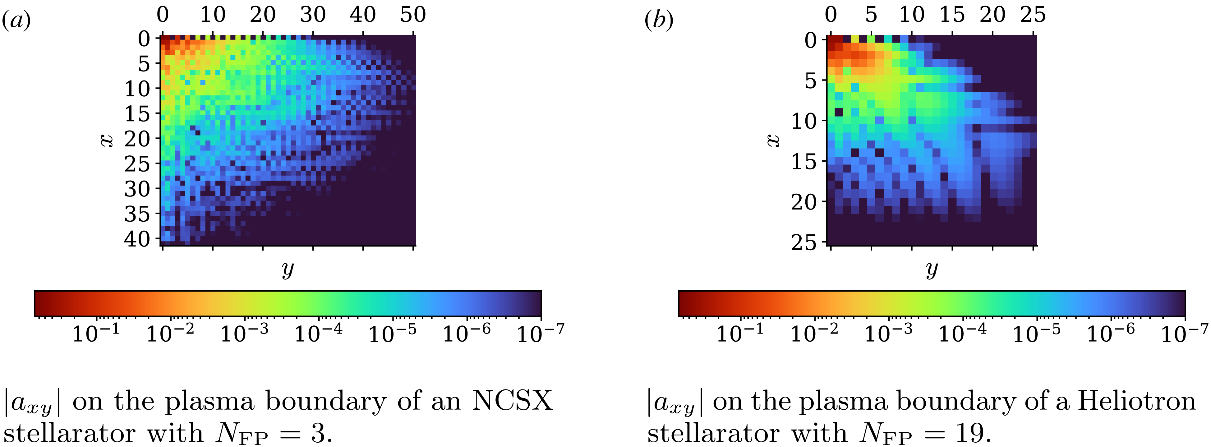 $\theta$
on the plasma boundary of an NCSX stellarator with
$\theta$
on the plasma boundary of an NCSX stellarator with $N_{\text{FP}} = 3$
.
$N_{\text{FP}} = 3$
.
This approach avoids issues that result from changing the basis for $(R, Z, \varLambda , \omega )$
at each optimisation step (Appendix D).
$(R, Z, \varLambda , \omega )$
at each optimisation step (Appendix D).
3.6. Jacobian of the map to the mesh of field lines
In this section, we explain how we accelerate the iterative solve discussed in the previous section throughout optimisation. To bypass differentiating the iterative solve, we write the tangent and adjoint methods directly (Sapienza et al. Reference Sapienza2025, §§ 3.3.3, 3.9.2). For this task, we leverage the implicit function theorem to differentiate solutions $\theta ^\star$
to (3.13) with respect to the optimisable parameters, denoted here with
$\theta ^\star$
to (3.13) with respect to the optimisable parameters, denoted here with $\boldsymbol{x}_{\text{opt}}$
. Define
$\boldsymbol{x}_{\text{opt}}$
. Define
 \begin{align} f \colon \boldsymbol{x}_{\text{opt}}, \theta \mapsto \theta + \varLambda - \iota (\zeta + \omega ) - \alpha . \end{align}
Let $(\boldsymbol{x}_{\text{opt}}^\star , \theta ^\star )$
satisfy
$(\boldsymbol{x}_{\text{opt}}^\star , \theta ^\star )$
satisfy $f(\boldsymbol{x}_{\text{opt}}^\star , \theta ^\star ) = 0$
,
$f(\boldsymbol{x}_{\text{opt}}^\star , \theta ^\star ) = 0$
,
 \begin{equation} \frac {\partial {f}}{\partial {\theta }}(\boldsymbol{x}_{\text{opt}}^\star , \theta ^\star ) = 1 + \frac {\partial {(\varLambda - \iota \omega )}}{\partial {\theta }}(\boldsymbol{x}_{\text{opt}}^\star , \theta ^\star ) \underset {(3.13)}{=} \left ({\frac {\partial {\alpha }}{\partial {\theta }}}\right )_{\psi , \zeta }(\boldsymbol{x}_{\text{opt}}^\star , \theta ^\star ). \end{equation}
In the $(\psi , \alpha , \zeta )$
covariant basis, the only non-zero component of the non-vanishing magnetic field is (3.16), so the derivative (3.23) is invertible. By the implicit function theorem,
$(\psi , \alpha , \zeta )$
covariant basis, the only non-zero component of the non-vanishing magnetic field is (3.16), so the derivative (3.23) is invertible. By the implicit function theorem, $\theta ^\star$
is a continuously differentiable map of
$\theta ^\star$
is a continuously differentiable map of $\boldsymbol{x}_{\text{opt}}$
and
$\boldsymbol{x}_{\text{opt}}$
and $f(\boldsymbol{x}_{\text{opt}}, \theta ^\star (\boldsymbol{x}_{\text{opt}})) = 0$
near
$f(\boldsymbol{x}_{\text{opt}}, \theta ^\star (\boldsymbol{x}_{\text{opt}})) = 0$
near $\boldsymbol{x}_{\text{opt}}^\star$
. Moreover,
$\boldsymbol{x}_{\text{opt}}^\star$
. Moreover,
 \begin{equation} \frac {\partial {\theta ^\star }}{\partial {\boldsymbol{x}_{\text{opt}}}}(\boldsymbol{x}_{\text{opt}}) = -\left [{\frac {\partial {f}}{\partial {\theta }}(\boldsymbol{x}_{\text{opt}}, \theta ^\star (\boldsymbol{x}_{\text{opt}}))}\right ]^{-1} \frac {\partial {f}}{\partial {\boldsymbol{x}_{\text{opt}}}}(\boldsymbol{x}_{\text{opt}}, \theta ^\star (\boldsymbol{x}_{\text{opt}})). \end{equation}
Thus, we differentiate directly through the solution $\theta ^\star$
. Likewise, after updating
$\theta ^\star$
. Likewise, after updating $\boldsymbol{x}_{\text{opt}}$
, we use (3.24) to warm start the next Newton iteration at an initial value that is correct to first order.
$\boldsymbol{x}_{\text{opt}}$
, we use (3.24) to warm start the next Newton iteration at an initial value that is correct to first order.
4. Optimisation for reduced neoclassical transport
We present an optimisation starting from a finite-beta helically omnigenous (OH) equilibrium. Finite-beta refers to the non-zero ratio of plasma pressure and magnetic pressure. We target flux surfaces near the boundary to reduce the effective ripple while maintaining reasonable elongation and curvature. With weights, $w_{\mathrm{A}}, w_{\mathrm{C}}, w_{\mathrm{E}}, w_{\mathrm{O}}, w_{\mathrm{R}}$
, the objective (4.1) is minimised while ensuring ideal MHD force balance (3.11) is maintained,
$w_{\mathrm{A}}, w_{\mathrm{C}}, w_{\mathrm{E}}, w_{\mathrm{O}}, w_{\mathrm{R}}$
, the objective (4.1) is minimised while ensuring ideal MHD force balance (3.11) is maintained,
 \begin{equation} w_{\mathrm{A}} f_{\mathrm{aspect}}^2 + w_{\mathrm{C}} f_{\mathrm{curv}}^2 + w_{\mathrm{E}} f_{\mathrm{elongation}}^2 + w_{\mathrm{O}} f_{\mathrm{omni}}^2 + w_{\mathrm{R}} f_{\mathrm{ripple}}^2. \end{equation}
The initial equilibrium along with the definitions of the curvature and elongation objectives are provided by Gaur et al. (Reference Gaur, Conlin, Dickinson, Parisi, Panici, Dudt, Kim, Unalmis, Dorland and Kolemen2025a ) and Gaur (Reference Gaur2024). The results are presented in figure 9. The optimisation took less than two hours with a GPU (NVIDIA Corporation 2020).
An OH transport optimisation. Panels (b) and (c) are shown in Boozer coordinates (D’haeseleer et al. Reference D’haeseleer, Hitchon, Callen and Shohet2012). Panels (d) and (e) show bounce-averaged radial drifts, summed in magnitude over $\zeta \in (0, 2\mathrm{\pi })$
. The size of the region with large drifts appears reduced.
$\zeta \in (0, 2\mathrm{\pi })$
. The size of the region with large drifts appears reduced.
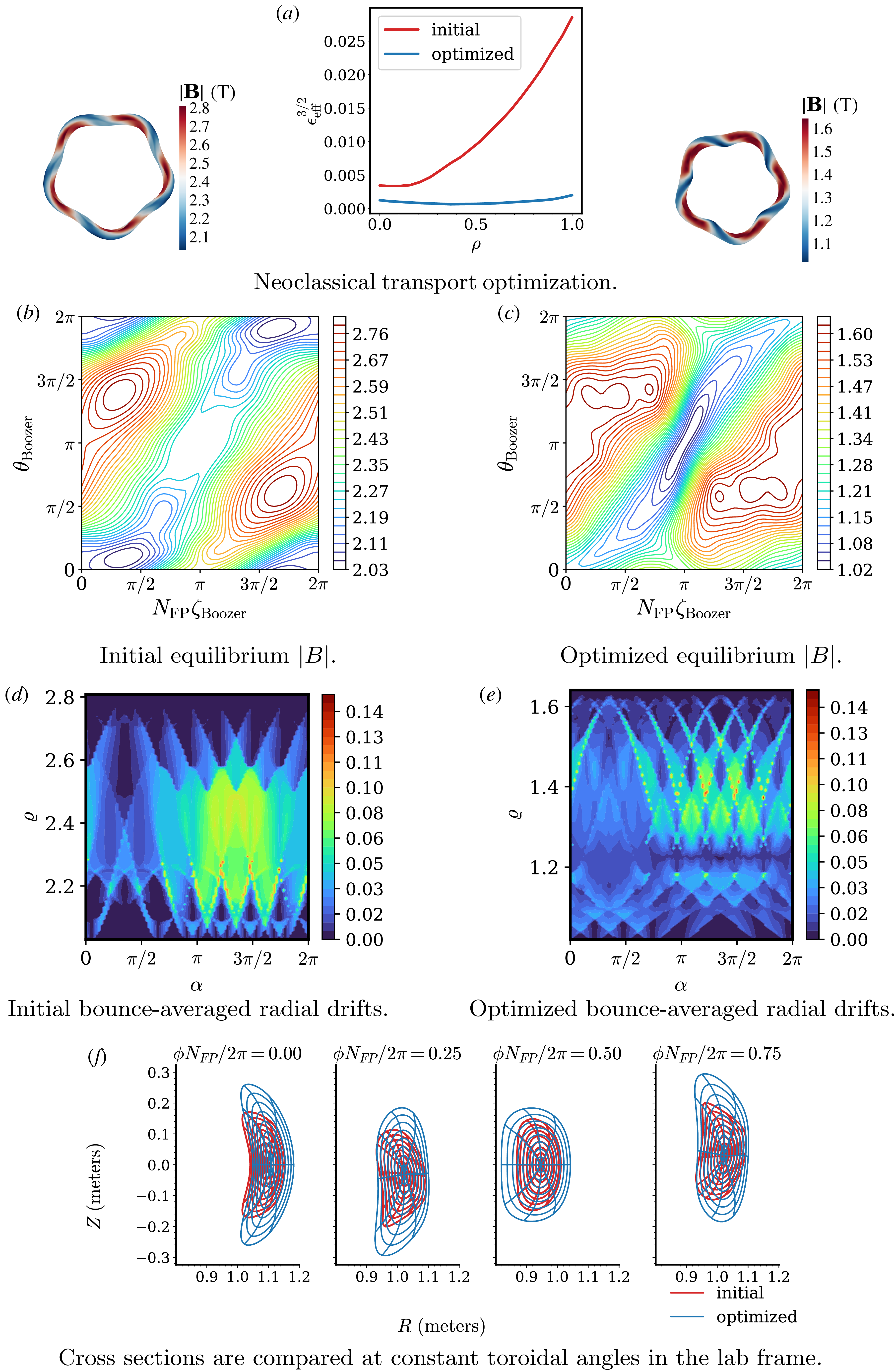
The omnigeneity objective is based on the work of Dudt et al. (Reference Dudt, Goodman, Conlin, Panici and Kolemen2024), where it was shown that optimising for omnigeneity can in turn reduce the effective ripple. Directly optimising to reduce the effective ripple instead has the advantage that the optimiser is not biased towards a user-specified omnigenous field. For example, in Gaur et al. (Reference Gaur, Panici, Elder, Landreman, Unalmis, Elmacioglu, Dudt, Conlin and Kolemen2025b ), we used this property to optimise for an umbilic boundary, while maintaining a low effective ripple without biasing the optimiser towards an omnigenous field with a specific helicity.
It should be noted that the assumptions used to derive the effective ripple increase in validity as the magnetic field becomes more omnigenous. For example, bounce-averaging assumes the radial orbit width is small compared with the magnetic field gradient scale length $\Delta r \ll L_{B}$
. When finite orbit width effects become dominant (d’Herbemont et al. Reference d’Herbemont, Parra, Calvo and Velasco2022), particles may traverse ‘potato’ orbits requiring a more global treatment (Satake, Okamoto & Sugama Reference Satake, Okamoto and Sugama2002). Hence, there is utility in optimisation that uses both objectives, either simultaneously or in succession.
$\Delta r \ll L_{B}$
. When finite orbit width effects become dominant (d’Herbemont et al. Reference d’Herbemont, Parra, Calvo and Velasco2022), particles may traverse ‘potato’ orbits requiring a more global treatment (Satake, Okamoto & Sugama Reference Satake, Okamoto and Sugama2002). Hence, there is utility in optimisation that uses both objectives, either simultaneously or in succession.
5. Conclusions
In this work, we optimised a finite-beta configuration to directly reduce neoclassical transport using reverse-mode differentiation. More generally, we upgraded the DESC stellarator optimisation suite for fast, accurate, automatically differentiable bounce-averaging. We discussed how we perform moving-grid interpolation without sacrificing spectral accuracy. This accuracy ensures that changes in the objective due to small changes in controllable parameters reflect genuine improvement or degradation rather than noise due to error. Therefore, optimisation is more likely to be successful.
Our algorithm enables optimisation for many objectives to improve stellarator performance. These include maximisation of the second adiabatic invariant (Helander Reference Helander2014, § 3.7; Rodríguez et al. Reference Rodríguez, Helander and Goodman2024), energetic particle confinement (Nemov et al. Reference Nemov, Kasilov, Kernbichler and Leitold2008; Velasco et al. Reference Velasco, Mulas and Cappa2021a ) and proxies for gyrokinetic turbulence such as the available energy (Mackenbach, Proll & Helander Reference Mackenbach, Proll and Helander2022; Mackenbach et al. Reference Mackenbach, Proll, Wakelkamp and Helander2023a ). We have added all these objectives to DESC. Some of these objectives have previously had limited use in optimisation due to expensive computational requirements or difficulty finding desirable configurations. Further demonstration of optimisation with them remains as future work.
Acknowledgements
Editor Per Helander thanks the referees for their advice in evaluating this article.
Funding
This work is funded through the SciDAC program by the US Department of Energy, Office of Fusion Energy Science, and Office of Advanced Scientific Computing Research under contract numbers DE-AC02-09CH11466, DE-SC0022005, and Field Work Proposal No. 1019. This work was also funded by the Peter B. Lewis Fund for Student Innovation in Energy and the Environment. This research used the resources of the Della computing cluster at Princeton University.
Declaration of interests
The authors declare no competing interests.
Author Contributions
Kaya Unalmis: Conceptualization; Methodology; Formal analysis; Investigation; Software; Validation; Visualization; Data curation; Writing - original draft; Writing - review & editing.
Rahul Gaur: Formal analysis; Software; Writing - review & editing.
Rory Conlin: Methodology; Software.
Dario Panici: Writing - review & editing.
Egemen Kolemen: Supervision; Writing - review & editing; Funding acquisition; Project administration.
Appendix A. Open source code
The implementation and supplementary information describing how correctness of automatic differentiation is enforced may be found in the DESC repository (Dudt et al. Reference Dudt, Conlin, Panici, Unalmis, Elmacioglu, Gaur, Kim and Kolemen2025). The implementation uses accelerated linear algebra XLA and Google’s JAX library (Bradbury et al. Reference Bradbury2018). JIT compilation in JAX compiles the code at the start of an optimisation. Optimisation may be accelerated on CPUs, GPUs and TPUs.
Appendix B. Effective ripple
We explain a short derivation of $\epsilon _{\text{eff}}$
, similar to the one used by Nemov et al. (Reference Nemov, Kasilov, Kernbichler and Heyn1999).
$\epsilon _{\text{eff}}$
, similar to the one used by Nemov et al. (Reference Nemov, Kasilov, Kernbichler and Heyn1999).
To obtain an explicit expression for $\varGamma$
, we will bounce-integrate the drift-kinetic equation (2.4). Applying this operator to the drift-kinetic equation discretises the spatial coordinate
$\varGamma$
, we will bounce-integrate the drift-kinetic equation (2.4). Applying this operator to the drift-kinetic equation discretises the spatial coordinate $\zeta$
to a set of integral equations labelled by the magnetic well index
$\zeta$
to a set of integral equations labelled by the magnetic well index $w$
.
$w$
.
The collision operator in (2.4) is chosen to capture pitch angle scattering,
 \begin{equation} \mathcal{C}[f] = \nu m \frac {\lvert {v_{\parallel }}\rvert }{\lvert {B}\rvert } \frac {\partial }{\partial \mu } \left ({\mu \lvert {v_{\parallel }}\rvert \frac {\partial f}{\partial \mu }}\right ) .\end{equation}
These derivatives are at fixed position and energy. The collision frequency $\nu$
depends only on the energy of the particle. The velocity ratio is
$\nu$
depends only on the energy of the particle. The velocity ratio is $\lvert {v_{\parallel }}\rvert / \lvert {v}\rvert = (1 - \lvert {B}\rvert / \varrho )^{1/2}$
. The nullspace of this collision operator contains velocity-isotropic distributions, so
$\lvert {v_{\parallel }}\rvert / \lvert {v}\rvert = (1 - \lvert {B}\rvert / \varrho )^{1/2}$
. The nullspace of this collision operator contains velocity-isotropic distributions, so $\mathcal{C}[f_0 + f_1] = \mathcal{C}[f_1]$
. In this form, (2.4) is the linearised Lorentz-gas Fokker–Planck equation (Goldston & Rutherford Reference Goldston and Rutherford1995, § 13).
$\mathcal{C}[f_0 + f_1] = \mathcal{C}[f_1]$
. In this form, (2.4) is the linearised Lorentz-gas Fokker–Planck equation (Goldston & Rutherford Reference Goldston and Rutherford1995, § 13).
In weakly collisional plasmas, the collision frequency is small compared with the particle bounce frequency. Consequently, fluctuations due to collisions homogenise along field lines rapidly, implying that the spatial variation in the plasma distribution along field lines in any particular magnetic well is small. Therefore, we approximate $f_0$
and
$f_0$
and $f_1$
to be spatially uniform along field lines in any particular magnetic well,
$f_1$
to be spatially uniform along field lines in any particular magnetic well,
 \begin{align} \boldsymbol{\nabla } f = \left ({\frac {\partial {f}}{\partial {\psi }}}\right )_{\alpha , \zeta , E, \mu } \boldsymbol{\nabla } \psi + \left ({\frac {\partial {f}}{\partial {\alpha }}}\right )_{\psi , \zeta , E, \mu } \boldsymbol{\nabla } \alpha + \left ({\frac {\partial {f}}{\partial {\zeta }}}\right )_{\psi ,\alpha , E, \mu } \boldsymbol{\nabla } \zeta, \end{align}
 \begin{align} \lvert {\boldsymbol{\nabla } f}\rvert \gg \lvert {(\partial f / \partial \zeta ) \boldsymbol{\nabla } \zeta }\rvert .\end{align}
Nested flux surfaces (2.1) then imply the parallel drift $\boldsymbol{v}_{\mathrm{Ba}\tilde{\mathrm{n}}\mathrm{os}}$
and the parallel spatial derivative of
$\boldsymbol{v}_{\mathrm{Ba}\tilde{\mathrm{n}}\mathrm{os}}$
and the parallel spatial derivative of $f_1$
will be negligible in the bounce-integrated drift-kinetic equation,
$f_1$
will be negligible in the bounce-integrated drift-kinetic equation,
 \begin{align} \overline {\mathcal{C}[f_1]} & = \nu m \frac {\partial }{\partial \mu } \mu \int \frac {\mathrm{d} \zeta }{\boldsymbol{b} \boldsymbol{\cdot }\boldsymbol{\nabla } \zeta } \frac {\lvert {v_{\parallel }}\rvert }{\lvert {B}\rvert } \frac {\partial {f_1}}{\partial {\mu }} \nonumber \\[5pt] & = \nu m \frac {\partial }{\partial \mu } \mu \frac {\partial {f_1}}{\partial {\mu }} \overline {\lvert {v_{\parallel }}\rvert ^2 / \lvert {B}\rvert } \nonumber \\[5pt] & = \frac {\partial f_0}{\partial \psi } \overline {\boldsymbol{v}_{\mathrm{D}s}\boldsymbol{\cdot }\boldsymbol{\nabla } \psi }. \end{align}
To write the last relation (B4), we assume there are sufficiently many passing particles so that $f_0$
is independent of
$f_0$
is independent of $\alpha$
.Footnote
2
We proceed to invert the collision operator. First, label the geodesic curvature of the field line,
$\alpha$
.Footnote
2
We proceed to invert the collision operator. First, label the geodesic curvature of the field line,
 \begin{equation} \kappa _{\mathrm{G}} = \left [{\boldsymbol{b} \times (\boldsymbol{b}\boldsymbol{\cdot }\boldsymbol{\nabla } \boldsymbol{b})}\right ] \boldsymbol{\cdot }\frac {\boldsymbol{\nabla } \psi }{\lvert {\boldsymbol{\nabla } \psi }\rvert } = \frac {\boldsymbol{b} \times \boldsymbol{\nabla } \lvert {B}\rvert }{\lvert {B}\rvert } \boldsymbol{\cdot }\frac {\boldsymbol{\nabla } \psi }{\lvert {\boldsymbol{\nabla } \psi }\rvert }. \end{equation}
The second equality is a consequence of ideal MHD force balance (3.11). Now, the primitive with respect to $\mu$
of the bounce-integrated radial drift velocity is identified as follows:
$\mu$
of the bounce-integrated radial drift velocity is identified as follows:
 \begin{align} \frac {\partial }{\partial \mu } \overline {\lvert {v_{\parallel }}\rvert \beta } & = \overline {\boldsymbol{v}_{\mathrm{D}s}\boldsymbol{\cdot }\boldsymbol{\nabla } \psi },\\[-10pt]\nonumber \end{align}
 \begin{align} \frac {\partial {\beta }}{\partial {\mu }} & = \frac {\boldsymbol{v}_{\mathrm{D}s}\boldsymbol{\cdot }\boldsymbol{\nabla } \psi }{\lvert {v_{\parallel }}\rvert } = (\lvert {v}\rvert ^2 \lvert {v_{\parallel }}\rvert ^{-1} + \lvert {v_{\parallel }}\rvert ) \frac {\lvert {\boldsymbol{\nabla } \psi }\rvert \kappa _{\mathrm{G}}}{2 \varOmega _s},\\[-10pt]\nonumber \end{align}
 \begin{align} \beta & = - (3 \lvert {v}\rvert ^2 \lvert {v_{\parallel }}\rvert + \lvert {v_{\parallel }}\rvert ^3) \frac {m \lvert {\boldsymbol{\nabla } \psi }\rvert \kappa _{\mathrm{G}}}{6 \varOmega _s \lvert {B}\rvert }.\\[6pt]\nonumber \end{align}
Inverting the $\mu$
derivative in (B4) completes the inversion of the collision operator,
$\mu$
derivative in (B4) completes the inversion of the collision operator,
 \begin{gather} \nu m \frac {\partial }{\partial \mu } \left ({\mu \frac {\partial f_1}{\partial \mu } \overline {\lvert {v_{\parallel }}\rvert ^2 / \lvert {B}\rvert }}\right ) = \frac {\partial }{\partial \mu } \left ({ \frac {\partial f_0}{\partial \psi } \overline {\lvert {v_{\parallel }}\rvert \beta }}\right ) \nonumber \\[6pt] \frac {\partial f_1}{\partial \mu } = \frac {\partial f_0}{\partial \psi } \frac {\overline {\lvert {v_{\parallel }}\rvert \beta }}{\nu m \mu \overline {\lvert {v_{\parallel }}\rvert ^2 / \lvert {B}\rvert }}. \end{gather}
To compute (2.6), we will use the $(E, \mu )$
parametrisation of velocity space,
$(E, \mu )$
parametrisation of velocity space,
 \begin{align} \int \mathrm{d}{^3\boldsymbol{v}} & = \frac {2\mathrm{\pi }}{m^2} \lvert {B}\rvert \int _{0}^{\infty } \mathrm{d} E \int _{0}^{E / \lvert {B}\rvert } \frac {\mathrm{d} \mu }{\lvert {v_{\parallel }}\rvert }\\[-10pt]\nonumber\end{align}
 \begin{align} & = \frac {2^{1/2} \mathrm{\pi }}{m^{3/2}} \lvert {B}\rvert \int _{0}^{\infty } \mathrm{d} E \; E^{1/2} \int _{\lvert {B}\rvert }^{\infty } \frac {\mathrm{d} \varrho }{\varrho ^{2} (1- \lvert {B}\rvert / \varrho )^{1/2}}.\end{align}
The plasma distribution vanishes where $\mu \geqslant E / \lvert {B}\rvert$
, so the integration region was truncated. Using (B10), applying integration by parts in the
$\mu \geqslant E / \lvert {B}\rvert$
, so the integration region was truncated. Using (B10), applying integration by parts in the $\mu$
coordinate and enforcing the boundary condition
$\mu$
coordinate and enforcing the boundary condition $\lim _{\mu \to 0} f_1 = 0$
at fixed energy, the radial particle flux density (2.6) can be written in terms of known quantities as follows:
$\lim _{\mu \to 0} f_1 = 0$
at fixed energy, the radial particle flux density (2.6) can be written in terms of known quantities as follows:
 \begin{equation} \varGamma = - \int \mathrm{d}{^3\boldsymbol{v}} \; \lvert {v_{\parallel }}\rvert \beta \frac {\partial f_1}{\partial \mu }. \end{equation}
To make optimisation efficient, the flux surface average of the radial particle flux density is of interest to minimise. This is the average on an infinitesimal volume covering the surface,
 \begin{equation} \langle \varGamma \rangle = \left ({\int \frac {\mathrm{d} s}{\lvert {\boldsymbol{\nabla } \psi }\rvert } \varGamma }\right ) \left ({\int \frac {\mathrm{d} s}{\lvert {\boldsymbol{\nabla } \psi }\rvert }}\right )^{-1}. \end{equation}
Here, $\mathrm{d} s$
is the differential surface area Jacobian. As (B12) enables computing the radial particle flux density through a quotient of bounce integrals along the magnetic field line (B9), it is more tractable to also compute the flux surface average along the field line,
$\mathrm{d} s$
is the differential surface area Jacobian. As (B12) enables computing the radial particle flux density through a quotient of bounce integrals along the magnetic field line (B9), it is more tractable to also compute the flux surface average along the field line,
 \begin{equation} \langle \varGamma \rangle = \left ({ \int _{0}^{2 \mathrm{\pi }} \mathrm{d} \alpha \int _{\mathbb{R}} \frac {\mathrm{d} \zeta }{\boldsymbol{B} \boldsymbol{\cdot }\boldsymbol{\nabla } \zeta } \varGamma }\right ) \left ({\int _{0}^{2 \mathrm{\pi }} \mathrm{d} \alpha \int _{\mathbb{R}} \frac {\mathrm{d} \zeta }{\boldsymbol{B} \boldsymbol{\cdot }\boldsymbol{\nabla } \zeta }}\right )^{-1}. \end{equation}
We proceed to extract a dimensionless quantity $\varGamma _0$
for the optimisation objective. First, we use (B11) and (B14) to remove the spatial dependence in the boundary of the velocity integral,
$\varGamma _0$
for the optimisation objective. First, we use (B11) and (B14) to remove the spatial dependence in the boundary of the velocity integral,
 \begin{align} \langle \varGamma \rangle & =- \frac {2 \mathrm{\pi }}{m^2} \left ({\int _{0}^{2 \mathrm{\pi }} \mathrm{d} \alpha \int _{0}^{\infty } \mathrm{d} E \; E \int _{\mathbb{R}}\frac {\mathrm{d} \zeta }{\boldsymbol{b} \boldsymbol{\cdot }\boldsymbol{\nabla } \zeta } \; \int _{\lvert {B}\rvert }^{\infty } \frac {\mathrm{d} \varrho }{\varrho ^{2}} \; \beta \frac {\partial f_1}{\partial \mu } }\right ) \left ({\int _{0}^{2 \mathrm{\pi }} \mathrm{d} \alpha \int _{\mathbb{R}} \frac {\mathrm{d} \zeta }{\boldsymbol{B} \boldsymbol{\cdot }\boldsymbol{\nabla } \zeta }}\right )^{-1} \nonumber \\[6pt] & =- \frac {2 \mathrm{\pi }}{m^2} \left ({\int _{0}^{2 \mathrm{\pi }} \mathrm{d} \alpha \int _{0}^{\infty } \mathrm{d} E \; E \int _{\lvert {B}\rvert _{\text{min}}}^{\lvert {B}\rvert _{\text{max}}} \frac {\mathrm{d} \varrho }{\varrho ^{2}} \sum _w \overline {\lvert {v_{\parallel }}\rvert \beta } \frac {\partial f_1}{\partial \mu }}\right ) \left ({\int _{0}^{2 \mathrm{\pi }} \mathrm{d} \alpha \int _{\mathbb{R}} \frac {\mathrm{d} \zeta }{\boldsymbol{B} \boldsymbol{\cdot }\boldsymbol{\nabla } \zeta }}\right )^{-1}. \end{align}
Here, $\lvert {B}\rvert _{\text{min}}$
and
$\lvert {B}\rvert _{\text{min}}$
and $\lvert {B}\rvert _{\text{max}}$
are the min and max values on the flux surface. The integral was truncated at
$\lvert {B}\rvert _{\text{max}}$
are the min and max values on the flux surface. The integral was truncated at $\lvert {B}\rvert _{\text{max}}$
as
$\lvert {B}\rvert _{\text{max}}$
as $f_1 = 0$
for passing particles. Now, changing coordinates in (B8),
$f_1 = 0$
for passing particles. Now, changing coordinates in (B8),
 \begin{equation} \beta = - \frac {(2 m E^3)^{1/2} c}{3 \varrho e \lvert {B}\rvert } (1 - \lvert {B}\rvert / \varrho )^{1/2} (4 \varrho / \lvert {B}\rvert - 1) \lvert {\boldsymbol{\nabla } \psi }\rvert \kappa _{\mathrm{G}} \end{equation}
and using the new partition for the velocity integral (B15), the expression (B14) may be approximated using a sum over all wells in the interval $[{\zeta _1, \zeta _2}]$
(2.7).
$[{\zeta _1, \zeta _2}]$
(2.7).
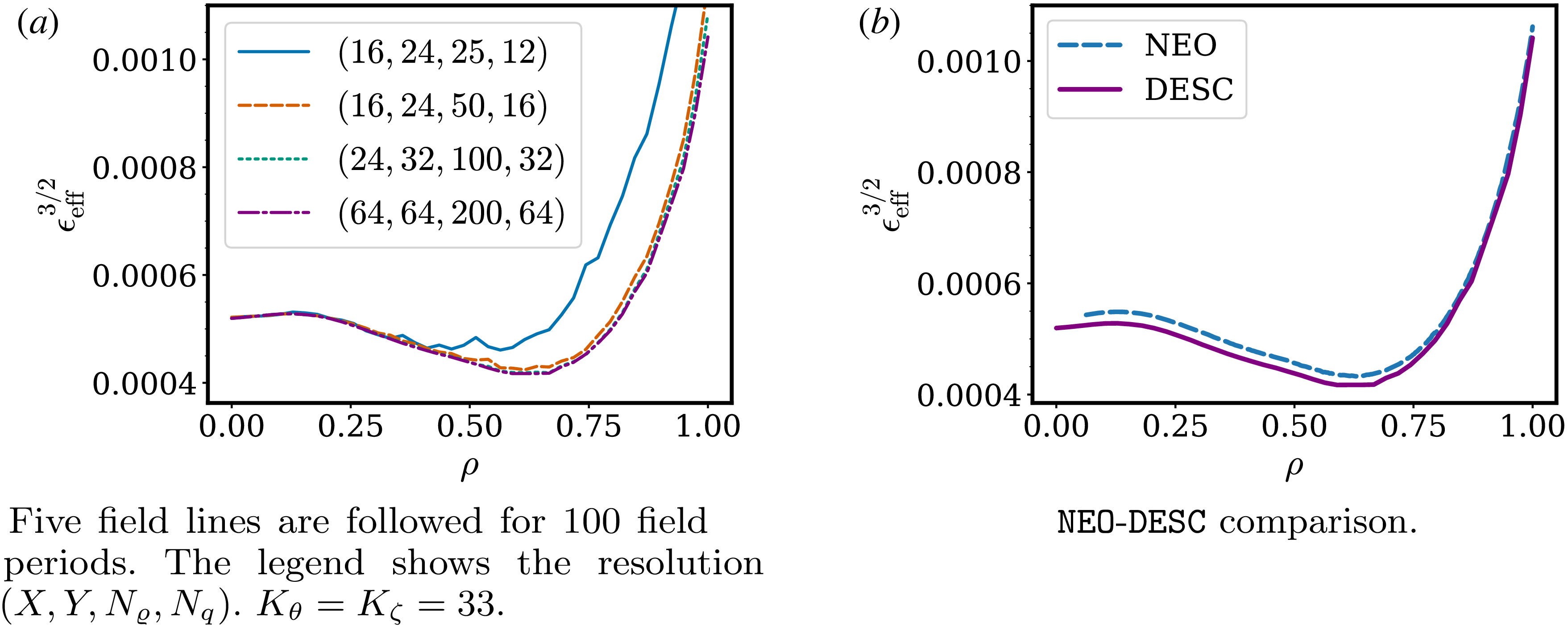
B.1 Resolution scan for the neoclassical transport coefficient
Figure 10(a) presents a resolution scan for $\epsilon _{\mathrm{eff}}$
. Figure 10(b) compares the result to the NEO code (Nemov et al. Reference Nemov, Kasilov, Kernbichler and Heyn1999), which uses a finite difference technique and requires transforming to Boozer coordinates. For the bounce integrals, NEO employs an explicit Runge–Kutta scheme which has algebraic convergence of order
$\epsilon _{\mathrm{eff}}$
. Figure 10(b) compares the result to the NEO code (Nemov et al. Reference Nemov, Kasilov, Kernbichler and Heyn1999), which uses a finite difference technique and requires transforming to Boozer coordinates. For the bounce integrals, NEO employs an explicit Runge–Kutta scheme which has algebraic convergence of order $1 + \eta/2$
for (3.3).
$1 + \eta/2$
for (3.3).
We mention some performance benchmarking of our algorithm in what follows. Computing $\epsilon _{\mathrm{eff}} \colon \mathbb{R}^{4074} \to \mathbb{R}^{10}$
and its derivative, on ten flux surfaces, following each field line for 75 field periods, with resolution
$\epsilon _{\mathrm{eff}} \colon \mathbb{R}^{4074} \to \mathbb{R}^{10}$
and its derivative, on ten flux surfaces, following each field line for 75 field periods, with resolution $(K_{\theta }, K_{\zeta }, X, Y, N_{\varrho }, N_{q}) = (32, 32, 32, 32, 100, 32)$
was profiled to take less than one and two seconds, respectively, with a CPU (Intel Corporation 2019), with peak memory consumption near one gigabyte. These computations are at least an order of magnitude faster with a GPU.
$(K_{\theta }, K_{\zeta }, X, Y, N_{\varrho }, N_{q}) = (32, 32, 32, 32, 100, 32)$
was profiled to take less than one and two seconds, respectively, with a CPU (Intel Corporation 2019), with peak memory consumption near one gigabyte. These computations are at least an order of magnitude faster with a GPU.
Resolution scan for $\epsilon _{\text{eff}}$
on the W7-X equilibrium in the DESC repository.
$\epsilon _{\text{eff}}$
on the W7-X equilibrium in the DESC repository.
Appendix C. Bounce-averaged drifts in a shifted-circle model
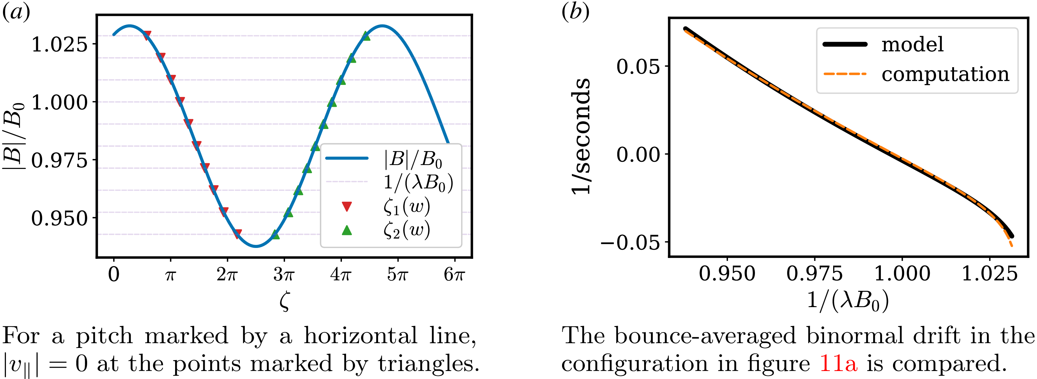
In a shifted-circle model for plasma equilibrium, we can obtain analytical expressions for bounce-averaged drifts. We further verify our algorithm with this model in figure 11.
Comparison of our shifted-circle model for the binormal drift with the result computed by our algorithm. The minor difference in panel (b) is because the shifted-circle model is accurate to $\mathcal{O}(\epsilon ^2)$
.
$\mathcal{O}(\epsilon ^2)$
.
In this model, the magnetic field can be written as
 \begin{equation} \boldsymbol{B} = \boldsymbol{\nabla } \alpha \times \boldsymbol{\nabla } \chi = F \boldsymbol{\nabla } \phi + \frac {\mathrm{d}{\chi }}{\mathrm{d}{\rho }} \frac {\rho }{R_0} \boldsymbol{\nabla } \vartheta, \end{equation}
where $\alpha = \phi - \iota ^{-1} \vartheta$
,
$\alpha = \phi - \iota ^{-1} \vartheta$
, $\chi$
is the poloidal flux,
$\chi$
is the poloidal flux, $F$
is the enclosed poloidal current,
$F$
is the enclosed poloidal current, $R_0$
is the average major radius and
$R_0$
is the average major radius and $\rho$
is a radial coordinate. To lowest order, the Grad–Shafranov equation has the constant solution
$\rho$
is a radial coordinate. To lowest order, the Grad–Shafranov equation has the constant solution $F = F_0$
. To the next order, the pressure gradient is
$F = F_0$
. To the next order, the pressure gradient is
 \begin{equation} \mathrm{d} p / \mathrm{d} \rho = - F_0 R^{-2} (\mathrm{d}{F} / \mathrm{d}{\rho }). \end{equation}
To first order, the poloidal magnetic field can be ignored so that the field satisfies $\lvert {B}\rvert = B_0 (1 - \epsilon \cos \vartheta )$
and
$\lvert {B}\rvert = B_0 (1 - \epsilon \cos \vartheta )$
and $\boldsymbol{b}\boldsymbol{\cdot }\boldsymbol{\nabla } \vartheta = G_0 (1-\epsilon \cos \vartheta )$
, where
$\boldsymbol{b}\boldsymbol{\cdot }\boldsymbol{\nabla } \vartheta = G_0 (1-\epsilon \cos \vartheta )$
, where $\epsilon \ll 1$
is the reciprocal of the aspect ratio. Here,
$\epsilon \ll 1$
is the reciprocal of the aspect ratio. Here, $B_0$
and
$B_0$
and $G_0$
are constants. In this model, the global shear
$G_0$
are constants. In this model, the global shear $\hat {s}$
, normalised pressure gradient and integrated local shear are
$\hat {s}$
, normalised pressure gradient and integrated local shear are
 \begin{align} \hat {s} & = - \rho \iota ^{-1} (\mathrm{d}{\iota } / \mathrm{d}{\rho }) ,\\[-10pt]\nonumber\end{align}
 \begin{align} \alpha _{\mathrm{MHD}} & = -2^{-1} \iota ^{-2} (\mathrm{d}{p} / \mathrm{d}{\rho }),\\[-10pt]\nonumber \end{align}
 \begin{align} \texttt {gds21} & = (\mathrm{d}{\chi } / \mathrm{d}{\rho }) (\mathrm{d}{\iota ^{-1}} / \mathrm{d}{\rho }) \boldsymbol{\nabla } \chi \boldsymbol{\cdot }\boldsymbol{\nabla } \alpha = -\hat {s} (\hat {s}\vartheta - \lvert {B}\rvert ^{-4} \alpha _{\mathrm{MHD}} \sin \vartheta ) + \mathcal{O}(\epsilon ).\\[6pt]\nonumber \end{align}
The binormal, geometric part of the $\boldsymbol{\nabla } \lvert {B}\rvert$
drift is
$\boldsymbol{\nabla } \lvert {B}\rvert$
drift is
 \begin{equation} (\boldsymbol{\nabla } \lvert {B}\rvert )_{\text{drift}} = \lvert {B}\rvert ^{-3} (\boldsymbol{B}\times \boldsymbol{\nabla } \lvert {B}\rvert ) \boldsymbol{\cdot }\boldsymbol{\nabla } \alpha = f_{2} (-\hat {{s}}+ \cos \vartheta - \hat {s}^{-1} {\texttt{gds21}} \sin \vartheta ). \end{equation}
The binormal, geometric part of the curvature drift is
 \begin{align} \texttt {cvdrift} & = \lvert {B}\rvert ^{-3} [\boldsymbol{B}\times \boldsymbol{\nabla } (p + \lvert {B}\rvert ^2 / 2) ] \boldsymbol{\cdot }\boldsymbol{\nabla } \alpha \nonumber \\ & = (\boldsymbol{\nabla } \lvert {B}\rvert )_{\text{drift}} +f_{3} \lvert {B}\rvert ^{-3} (\mathrm{d}{p} / \mathrm{d}{\rho }) \nonumber \\ & =f_{2} (-\hat {s}+ \cos \vartheta +\hat {s}\vartheta \sin \vartheta - B_0^{-4} \alpha _{\mathrm{MHD}} \sin ^2 \vartheta )+f_{3} B_0^{-2} \alpha _{\mathrm{MHD}} + \mathcal{O}(\epsilon ). \end{align}
The scalars $f_2$
and
$f_2$
and $f_3$
contain some constants. The bounce-averaged drift is
$f_3$
contain some constants. The bounce-averaged drift is
 \begin{equation} \langle v_{\mathrm{{D}}}\rangle = \left ({ \int _{\vartheta _1}^{\vartheta _2}\frac {\mathrm{d}\vartheta }{\boldsymbol{b}\boldsymbol{\cdot }\boldsymbol{\nabla }\vartheta }\lvert {v_{\parallel }}\rvert ^{-1} }\right )^{-1} \int _{\vartheta _1}^{\vartheta _2}\frac {\mathrm{d}\vartheta }{\boldsymbol{b}\boldsymbol{\cdot }\boldsymbol{\nabla }\vartheta } \left [{\lvert {v_{\parallel }}\rvert \texttt {cvdrift}+\frac {\lvert {v_{\perp }}\rvert ^{2}}{2 \lvert {v_{\parallel }}\rvert } (\boldsymbol{\nabla } \lvert {B}\rvert )_{\text{drift}}}\right ]. \end{equation}
As used by Connor, Hastie & Martin (Reference Connor, Hastie and Martin1983) and shown by Hegna (Reference Hegna2015), in the limit of a large aspect ratio shifted-circle model, the parallel speed of a particle with a fixed energy is $\ \lvert {v_{\parallel }}\rvert = (2E/m)^{1/2} (2\epsilon \lambda B_0)^{1/2} ({k^{2}-\sin ^2 (\vartheta /2)})^{1/2}$
, where
$\ \lvert {v_{\parallel }}\rvert = (2E/m)^{1/2} (2\epsilon \lambda B_0)^{1/2} ({k^{2}-\sin ^2 (\vartheta /2)})^{1/2}$
, where
 \begin{equation} k^{2}=2^{-1} [(1-\lambda B_{0})(\epsilon \lambda B_{0})^{-1} +1] \end{equation}
parametrises the pitch angle $\lambda$
. Using these simplifications and
$\lambda$
. Using these simplifications and $\lvert {v_{\perp }}\rvert ^2/2 = E/m - \lvert {v_{\parallel }}\rvert ^2/2$
,
$\lvert {v_{\perp }}\rvert ^2/2 = E/m - \lvert {v_{\parallel }}\rvert ^2/2$
,
 \begin{align} \langle v_{D}\rangle & = \left (\int _{-2\arcsin k}^{2\arcsin k}\frac {{\mathrm{d}\vartheta }}{\boldsymbol{b}\boldsymbol{\cdot }\boldsymbol{\nabla }\vartheta } (2 \epsilon \lambda B_0)^{-1/2} (k^{2}-\sin ^2(\vartheta /2))^{-1/2} \right )^{-1} \nonumber \\[4pt] & \quad \int _{-2\arcsin k}^{2\arcsin k}\frac {{\mathrm{d}\vartheta }}{\boldsymbol{b}\boldsymbol{\cdot }\boldsymbol{\nabla }\vartheta }\big [(2 \epsilon \lambda B_0)^{1/2} (k^{2}-\sin ^2(\vartheta /2))^{1/2} \texttt {cvdrift} \nonumber \\[4pt] & \qquad - 2^{-1/2} (\epsilon \lambda B_0)^{1/2} (k^{2}-\sin ^2(\vartheta /2))^{1/2} (\boldsymbol{\nabla } \lvert {B}\rvert )_{\text{drift}} \nonumber \\[4pt]& \qquad + 2^{-3/2} (\epsilon \lambda B_0)^{-1/2} (k^{2}-\sin ^2(\vartheta /2))^{-1/2} (\boldsymbol{\nabla } \lvert {B}\rvert )_{\text{drift}} \big ]. \end{align}
The following identities simplify (C10). The incomplete elliptic integrals are converted to complete elliptic integrals using the reciprocal-modulus transformation in (C11) and (C12) (Olver et al. Reference Olver2024). Here, $K$
and
$K$
and $E$
are complete elliptic integrals of the first and second kind, respectively,
$E$
are complete elliptic integrals of the first and second kind, respectively,
 \begin{align} \mathsf{I_{0}} & = \int _{-2\arcsin k}^{2\arcsin k} \mathrm{d}\vartheta \; ({k^{2}-\sin ^2 (\vartheta /2)})^{-1/2} = 4 K(k),\\[-10pt]\nonumber \end{align}
 \begin{align} \mathsf{I_{1}} & =\int _{-2\arcsin k}^{2\arcsin k}\mathrm{d}\vartheta \; ({k^{2}-\sin ^2 (\vartheta /2)})^{1/2} = 4 [E(k) + (k^2-1) K(k) ],\\[-10pt]\nonumber \end{align}
 \begin{align} \mathsf{I_{2}} & = \int _{-2\arcsin k}^{2\arcsin k} \mathrm{d}\vartheta \; (k^{2}-\sin ^2 (\vartheta /2))^{-1/2} \vartheta \sin \vartheta = 16 [E(k) + (k^2-1) K(k) ],\\[-10pt]\nonumber\end{align}
 \begin{align} \mathsf{I_{3}} & = \int _{-2\arcsin k}^{2\arcsin k} \mathrm{d}\vartheta \; ({k^{2}-\sin ^2 (\vartheta /2)})^{1/2} \vartheta \sin \vartheta =\frac {16}{9}[(4 k^2 - 2) E + (3 k^4 - 5 k^2 + 2)K],\\[-10pt]\nonumber \end{align}
 \begin{align} \mathsf{I_{4}} & = \int _{-2\arcsin k}^{2\arcsin k} \mathrm{d}\vartheta \; ({k^{2}-\sin ^2 (\vartheta /2)})^{-1/2} \sin ^2 \vartheta = \frac {16}{3} [(2k^2 -1) E + (1 - k^2) K ],\\[-10pt]\nonumber \end{align}
 \begin{align} \mathsf{I_{5}} & = \int _{-2\arcsin k}^{2\arcsin k} \mathrm{d}\vartheta \; (k^{2}-\sin ^2 (\vartheta /2))^{1/2} \sin ^2 \vartheta \nonumber \\[4pt] & \quad = \frac {32}{30} [ 2(1 - k^2 + k^4) (E + (k^2-1) K) - (1 - 3 k^2 + 2 k^4) k^2 K ],\\[-10pt]\nonumber \end{align}
 \begin{align} \mathsf{I_{6}} & = \int _{-2\arcsin k}^{2\arcsin k} \mathrm{d} \vartheta \; (k^{2}-\sin ^2 (\vartheta /2))^{-1/2} \cos \vartheta = 8 E - 4 K,\\[-10pt]\nonumber \end{align}
 \begin{align} \mathsf{I_{7}} & = \int _{-2\arcsin k}^{2\arcsin k} \mathrm{d} \vartheta \; (k^{2}-\sin ^2 (\vartheta /2))^{1/2} \cos \vartheta =\frac {4}{3} [(2k^2-1) E - (k^2-1) K ].\\[6pt]\nonumber \end{align}
Using these formulae with $\epsilon _{\lambda}= 2\epsilon\lambda B_0$
, to lowest order, the bounce-averaged drift is
$\epsilon _{\lambda}= 2\epsilon\lambda B_0$
, to lowest order, the bounce-averaged drift is
 \begin{align} \langle v_{D}\rangle & = \frac {1}{\mathsf{I}_{0}} \!\left [\!{f_3 \frac {\alpha _{\mathrm{MHD}}}{B_0^2} \epsilon_\lambda\mathsf{I}_1 {\kern-.5pt}- \frac {f_2}{2} \!\left (\!{\hat {s} ( \mathsf{I}_0 + \epsilon_\lambda\mathsf{I}_1 {\kern-.5pt}- \mathsf{I}_2 {\kern-.5pt}- \epsilon_\lambda\mathsf{I}_3 ) + \frac { \alpha _{\mathrm{MHD}}}{B_0^4} (\mathsf{I}_{4} {\kern-.5pt}+ \epsilon_\lambda\mathsf{I}_{5}) - (\mathsf{I}_{6} {\kern-.5pt}+ \epsilon_\lambda\mathsf{I}_{7})}\!\right )}\!\right ]\!.\nonumber \\ \end{align}
Error induced by changing the Fourier–Zernike basis for $(R, Z, \varLambda , \omega )$
from flux coordinates
$(R, Z, \varLambda , \omega )$
from flux coordinates $(\theta , \zeta )$
to the straight field line coordinates
$(\theta , \zeta )$
to the straight field line coordinates $(\vartheta , \phi )$
. Fitting at the resolution that obtains the error of
$(\vartheta , \phi )$
. Fitting at the resolution that obtains the error of $10^{-4}$
Tesla in
$10^{-4}$
Tesla in $\lvert {B}\rvert$
on the NCSX stellarator in panel (a) took 10 minutes with a CPU (Intel Corporation 2019).
$\lvert {B}\rvert$
on the NCSX stellarator in panel (a) took 10 minutes with a CPU (Intel Corporation 2019).

Appendix D. Issues with changing the spectral basis to straight field line coordinates
In figure 12, we show that parametrising our basis for $(R, Z, \varLambda , \omega )$
in straight field line coordinates
$(R, Z, \varLambda , \omega )$
in straight field line coordinates $(\vartheta , \phi ) = (\theta + \varLambda , \zeta + \omega )$
(Grimm, Greene & Johnson Reference Grimm, Greene and Johnson1976) is inefficient and ill-conditioned. Therefore, we use the approach discussed in the main text instead.
$(\vartheta , \phi ) = (\theta + \varLambda , \zeta + \omega )$
(Grimm, Greene & Johnson Reference Grimm, Greene and Johnson1976) is inefficient and ill-conditioned. Therefore, we use the approach discussed in the main text instead.






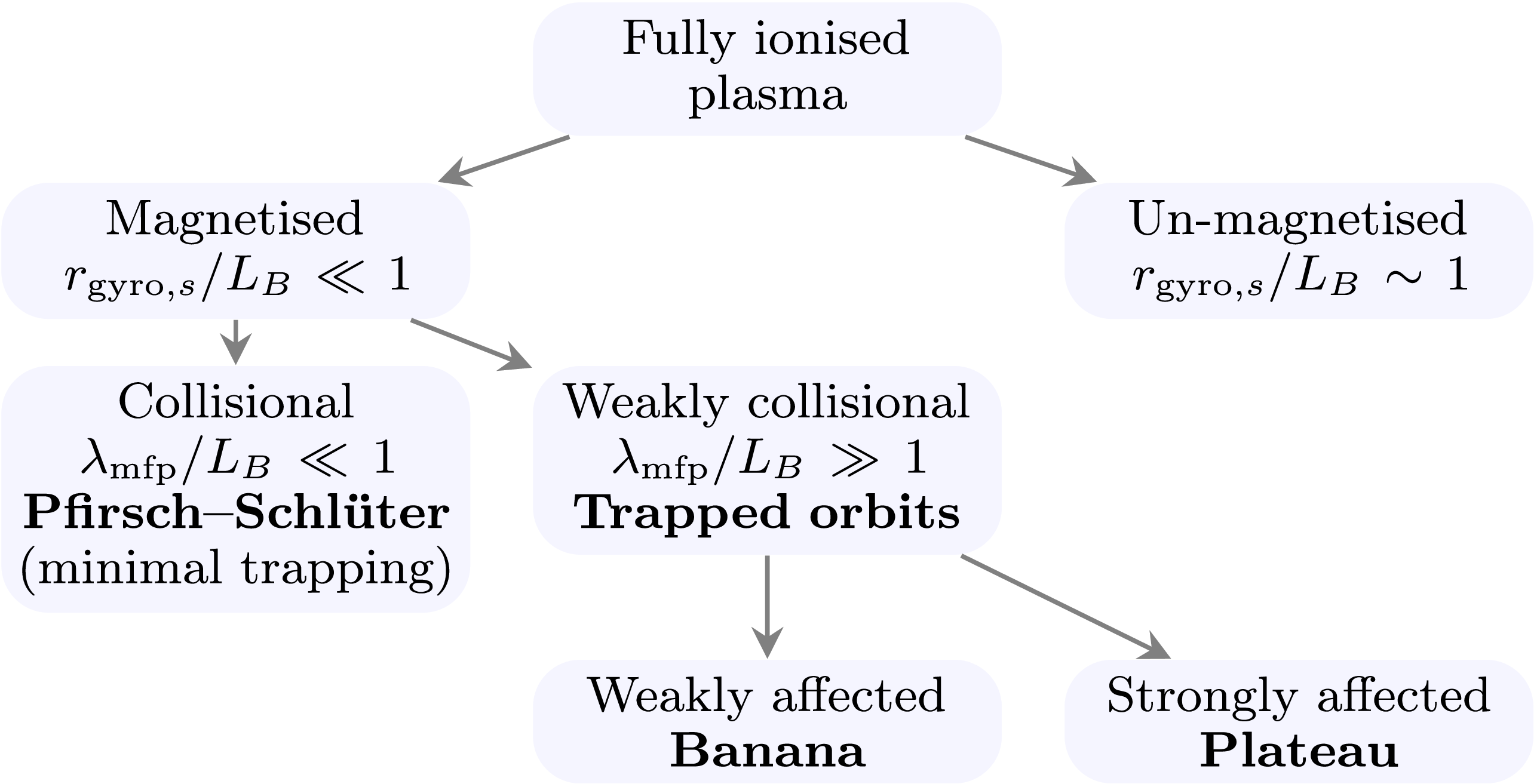
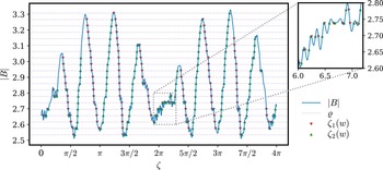


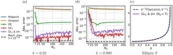


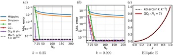


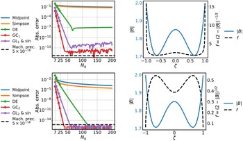

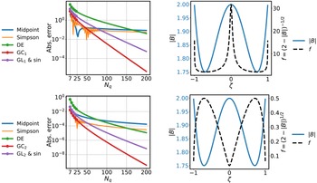


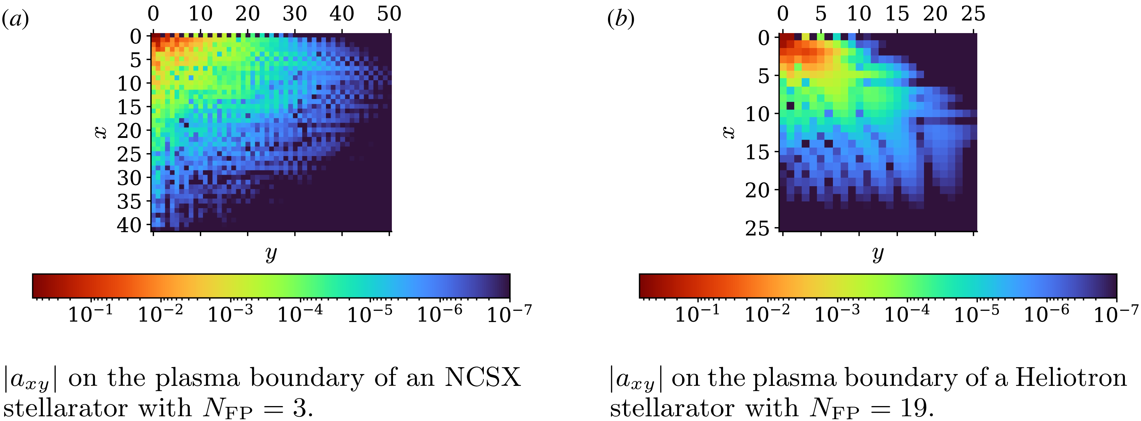


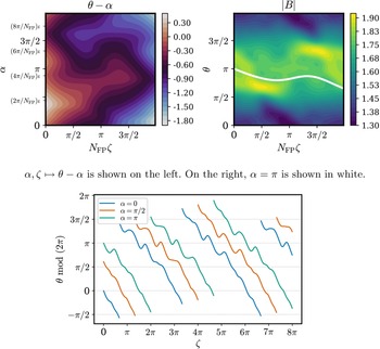


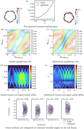

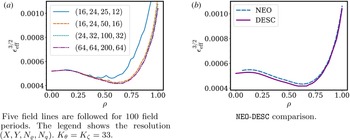

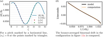

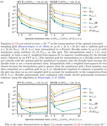


 Open access

