


1. Introduction
Marine macroalgae, such as kelp, provide essential habitats, shelter and food sources for a diverse range of marine species, with immense importance for biodiversity preservation and ecosystem health (e.g. Dayton Reference Dayton1985; Teagle et al. Reference Teagle, Hawkins, Moore and Smale2017). The cultivation and harvest of macroalgae also has the potential to become a sustainable strategy for biofuel production, food supply and carbon sequestration (Ghadiryanfar et al. Reference Ghadiryanfar, Rosentrater, Keyhani and Omid2016; Ferdouse et al. Reference Ferdouse, Holdt, Smith, Murúa and Yang2018). Given the constraints posed by the ecological carrying capacity of existing near-shore aquaculture, recent interest has thus arisen in expanding macroalgal farming offshore (Troell et al. Reference Troell, Joyce, Chopin, Neori, Buschmann and Fang2009; Yan, McWilliams & Chamecki Reference Yan, McWilliams and Chamecki2021; Frieder et al. Reference Frieder2022). These offshore macroalgal farms are usually attached to suspended structures near the ocean surface, typically within the ocean mixed layer (OML).
An essential factor affecting the performance of suspended macroalgal farms is their interaction with the hydrodynamic processes in the OML (Yan et al. Reference Yan, McWilliams and Chamecki2021; Frieder et al. Reference Frieder2022). Kelp exerts a drag force on the flow (e.g. Thom Reference Thom1971; Jackson Reference Jackson1997), resulting in attenuation in current velocity and wave motions (Rosman et al. Reference Rosman, Koseff, Monismith and Grover2007; Monismith et al. Reference Monismith, Alnajjar, Daly, Valle-Levinson, Juarez, Fagundes, Bell and Woodson2022). Discontinuities in drag can also lead to the development of shear layers and eddies at the boundaries of the canopy (Plew Reference Plew2011), which may cause significant modifications in OML turbulence (Yan et al. Reference Yan, McWilliams and Chamecki2021). These altered hydrodynamic conditions due to the presence of kelp can determine nutrient availability, chemical transport and salinity and temperature conditions in the farms, thereby affecting kelp growth.
Moreover, the variability of farm configurations, e.g. farm geometry and orientation with respect to currents and waves, can introduce added complexity into the interaction between kelp farms and OML turbulence. In addition, kelp growth and harvesting can effectively alter the frond surface area density (Frieder et al. Reference Frieder2022), consequently influencing the drag force and canopy flow profiles. A comprehensive understanding of the complex hydrodynamic processes in the OML with the presence of suspended farms is therefore crucial for optimally designing farm configurations and tactically managing harvesting practices.
The investigation of suspended farm hydrodynamics, beyond its direct implications for farm performance, also contributes to our broader understanding of how obstacle structures modify the OML. Various obstacle structures located near the ocean surface boundary, e.g. aquatic vegetation, engineered offshore platforms, ships, buoys and sea ice, have the potential to influence the hydrodynamic interactions among winds, waves and currents. These modifications to OML hydrodynamics may consequently result in alterations to other OML characteristics, e.g. heat transport and salinity mixing.
Suspended kelp farms, hydrodynamically classified as suspended canopies, share similarities with submerged canopies that are located on the bottom boundary (Plew Reference Plew2011; Tseung, Kikkert & Plew Reference Tseung, Kikkert and Plew2016). The emergence of shear layer turbulence at the top of the canopy has received considerable attention in the context of submerged canopy flow (e.g. Finnigan Reference Finnigan2000; Nepf Reference Nepf2012). Likewise, for a suspended canopy, a shear layer can develop at the bottom of the canopy, leading to generation of turbulence and the exchange of momentum and scalars between the canopy and the underlying flow (Plew Reference Plew2011). Additionally, for suspended canopies of finite dimensions, an adjustment region typically develops within the canopy starting from the leading edge (Tseung et al. Reference Tseung, Kikkert and Plew2016), where the flow adapts to the drag imposed by the canopy, similar to that of finite-length submerged canopies (Belcher, Jerram & Hunt Reference Belcher, Jerram and Hunt2003; Rominger & Nepf Reference Rominger and Nepf2011). Subsequent to this adjustment region, a fully developed canopy flow region emerges, followed by a wake region downstream from the canopy. While the suspended canopy in general behaves like an inverted submerged canopy (Plew Reference Plew2011), distinct hydrodynamic conditions can arise, as a result of the different boundary conditions at the surface and the prevalent presence of surface gravity waves in the OML.
A prominent turbulent process in the OML is the Langmuir circulation driven by wind and waves (e.g. Leibovich Reference Leibovich1983; McWilliams, Sullivan & Moeng Reference McWilliams, Sullivan and Moeng1997; Thorpe Reference Thorpe2004). It is typically visible on the ocean surface as streaks of foam or debris, i.e. surface convergence lines, and is usually roughly parallel to the directions of wind and waves (Langmuir Reference Langmuir1938). The generation of Langmuir circulation depends critically on the interaction between the sheared wind-driven current and the Stokes drift of surface gravity waves (e.g. Craik & Leibovich Reference Craik and Leibovich1976; Craik Reference Craik1977; Leibovich Reference Leibovich1977). Vorticity tilting due to the vertically sheared Stokes drift can cause instability to generate coherent Langmuir cell structures aligned with the downwind direction, and this is known as the Craik–Leibovich (CL) 2 mechanism. The intensified turbulence associated with Langmuir circulation can enhance the vertical transport and mixing in the upper ocean (McWilliams et al. Reference McWilliams, Sullivan and Moeng1997; McWilliams & Sullivan Reference McWilliams and Sullivan2000) and could even be important for producing and maintaining the uniform OML (Li & Garrett Reference Li and Garrett1997; Thorpe Reference Thorpe2004).
Nevertheless, the interplay between Langmuir turbulence and aquatic vegetation remains largely unexplored. The significance of Langmuir circulation extends beyond hydrodynamics, also playing a crucial role in biogeochemical transport in the OML and influencing the distribution of macroalgae (Evans & Taylor Reference Evans and Taylor1980; Dierssen et al. Reference Dierssen, Zimmerman, Drake and Burdige2009; Qiao et al. Reference Qiao, Dai, Simpson and Svendsen2009). On the other hand, the presence of vegetation can modify wind-driven currents and waves in the OML, and is thus expected to affect the generation of Langmuir turbulence. Yan et al. (Reference Yan, McWilliams and Chamecki2021) investigated the creation of attached Langmuir circulation in a suspended macroalgal farm with a specific configuration, where spaced rows of kelp are aligned parallel to the flow and waves. In addition to the generation of canopy shear layer turbulence below the farm, Langmuir-type turbulence was found to occur within the farm, with a stronger magnitude than the standard Langmuir turbulence generated without a farm. These various types of farm-generated turbulence can significantly affect nutrient transport in the OML, potentially leading to feedback on farm performance. Therefore, a more comprehensive examination of the physical mechanisms behind turbulence generation by suspended farms, e.g. the interaction between the Stokes drift and farm-modulated ocean currents, is necessary for an improved understanding of OML hydrodynamics. The dependence of canopy flow properties on different farm configurations also merits further investigation, as a crucial aspect of offshore farm planning and nutrient management.
In this study, we employ large eddy simulation (LES) to understand the influence of suspended kelp farms on OML hydrodynamics, with a particular focus on the mechanisms of turbulence generation. We also explore how varying farm configurations and frond density distributions affect these turbulence generation mechanisms. Section 2 describes the numerical method and the various farm configurations investigated in this study. Section 3 presents the statistics of mean flow, secondary flow and turbulence in the farm. In particular, we focus on three representative farm configurations to highlight the various flow patterns arising from different horizontal arrangements and vertical frond density profiles. Section 4 examines the energy budget to understand sources of farm-generated turbulence. Section 5 investigates the vorticity dynamics in the farm to illustrate the generation mechanisms of Langmuir circulations. In § 6, we explore other farm parameters that affect turbulence generation, including the effective frond area density, farm orientation and farm length. Section 7 presents the conclusion.
2. Methods
2.1. Model description
We use LES to investigate turbulence generation associated with suspended kelp farms. Large eddy simulation is a widely used tool in studying OML turbulence and more detailed discussion can be found in Chamecki et al. (Reference Chamecki, Chor, Yang and Meneveau2019). The code used in this study has been validated against Langmuir turbulence simulations in McWilliams et al. (Reference McWilliams, Sullivan and Moeng1997) and applied to previous research in the macroalgal farm and boundary layer flow (Yan et al. Reference Yan, McWilliams and Chamecki2021; Yan, McWilliams & Chamecki Reference Yan, McWilliams and Chamecki2022). The present LES framework is based on the wave-averaged and grid-filtered equations for mass, momentum and heat
 $$\begin{gather}
\boldsymbol{\nabla}\boldsymbol{\cdot}\tilde{\boldsymbol{u}}=0,\end{gather}$$
$$\begin{gather}
\boldsymbol{\nabla}\boldsymbol{\cdot}\tilde{\boldsymbol{u}}=0,\end{gather}$$
 $$\begin{gather}
\frac{\partial{\tilde{\boldsymbol{u}}}}{\partial{t}} +
\tilde{\boldsymbol{u}}\boldsymbol{\cdot}\boldsymbol{\nabla}\tilde{\boldsymbol{u}}
={-}\boldsymbol{\nabla}\varPi -
f\boldsymbol{e}_z\times\left(\tilde{\boldsymbol{u}} +
{\boldsymbol{u}}_s-{\boldsymbol{u}}_g\right)+
{\boldsymbol{u}}_s\times\tilde{\boldsymbol{\zeta}} \nonumber\\ \qquad\qquad\qquad\ +
\left(1-\frac{\tilde\rho}{\rho_0}\right)g\boldsymbol{e}_z -
\boldsymbol{\nabla}\boldsymbol{\cdot}\boldsymbol{\tau}^d -
\boldsymbol{F}_D,\end{gather}$$
$$\begin{gather}
\frac{\partial{\tilde{\boldsymbol{u}}}}{\partial{t}} +
\tilde{\boldsymbol{u}}\boldsymbol{\cdot}\boldsymbol{\nabla}\tilde{\boldsymbol{u}}
={-}\boldsymbol{\nabla}\varPi -
f\boldsymbol{e}_z\times\left(\tilde{\boldsymbol{u}} +
{\boldsymbol{u}}_s-{\boldsymbol{u}}_g\right)+
{\boldsymbol{u}}_s\times\tilde{\boldsymbol{\zeta}} \nonumber\\ \qquad\qquad\qquad\ +
\left(1-\frac{\tilde\rho}{\rho_0}\right)g\boldsymbol{e}_z -
\boldsymbol{\nabla}\boldsymbol{\cdot}\boldsymbol{\tau}^d -
\boldsymbol{F}_D,\end{gather}$$
 $$\begin{gather}\frac{\partial{\tilde{\theta}}}{\partial{t}}+\left(\tilde{\boldsymbol{u}} + {\boldsymbol{u}}_s\right) \boldsymbol{\cdot}\boldsymbol{\nabla}\tilde{\theta} ={-} \boldsymbol{\nabla}\boldsymbol{\cdot}\boldsymbol{\rm \pi}_\theta. \end{gather}$$
This mathematical model was initially introduced in McWilliams et al. (Reference McWilliams, Sullivan and Moeng1997) by extending the original CL equations (Craik & Leibovich Reference Craik and Leibovich1976), with the effects of planetary rotation and advection of scalars by Stokes drift incorporated.
The tilde in (2.1), (2.2) and (2.3) represents the grid-filtered variables. In the Cartesian coordinate system  $\boldsymbol {x} = (x,y,z)$, the velocity vector is $\tilde {\boldsymbol {u}}=(\tilde {u},\tilde {v},\tilde {w})$, i.e. the streamwise, lateral (cross-stream) and vertical components, respectively. In (2.2), $\varPi$ is the modified pressure (e.g. Chamecki et al. Reference Chamecki, Chor, Yang and Meneveau2019), $f$ is the Coriolis frequency, $g$ is the gravitational acceleration, $\boldsymbol {e}_z$ is the unit vector in the vertical direction and $\tilde {\boldsymbol {\zeta }} =\boldsymbol {\nabla }\times \tilde {\boldsymbol {u}}$ is the filtered vorticity. Here, $\boldsymbol {u}_s$ is the Stokes drift associated with surface gravity waves, and $\boldsymbol {u}_g$ is a geostrophic current that represents the effect of mesoscale ocean flows. The geostrophic current is driven by an external pressure gradient $f\boldsymbol {e}_z\times {\boldsymbol {u}}_g$. The term $\boldsymbol {F}_D$ represents the drag force imposed by the canopy onto the flow, and the detailed treatment of canopy drag will be described later.
In (2.2),  $\tilde {\rho }$ is the filtered density, and $\rho _0$ is the reference density. We assume that variations in density are only caused by the potential temperature $\tilde {\theta }$ via a linear relationship $\rho =\rho _0[1-\alpha (\theta -\theta _0)]$, where $\alpha =2\times 10^{-4}\,{\rm K}^{-1}$ is the thermal expansion coefficient and $\theta _0$ is the reference potential temperature corresponding to $\rho _0$. The term $\boldsymbol {\tau }^d$ is the deviatoric part of the subgrid-scale (SGS) stress tensor $\boldsymbol {\tau } = \widetilde {\boldsymbol {u}\boldsymbol {u}} - \tilde {\boldsymbol {u}}\,\tilde {\boldsymbol {u}}$, and $\boldsymbol {{\rm \pi} }_\theta =\widetilde {\boldsymbol {u}\theta }-\tilde {\boldsymbol {u}}\,\tilde {\theta }$ is the SGS heat flux. The SGS stress is modelled using the Lagrangian scale-dependent dynamic Smagorinsky model (Bou-Zeid, Meneveau & Parlange Reference Bou-Zeid, Meneveau and Parlange2005). The SGS heat flux is modelled using an eddy diffusivity closure, with diffusivity obtained from SGS viscosity and a prescribed value of turbulent Prandtl number $Pr_t = 0.4$. Molecular viscosity and diffusivity are assumed to be negligible for the high Reynolds number flows examined in this study.
The surface waves are not explicitly resolved in the model, and the time-averaged influences of waves are incorporated by imposing the Stokes drift  $\boldsymbol {u}_s$. We consider a simple case of monochromatic deep water wave propagating in the $x$ direction, with amplitude $a_w$ and frequency $\omega =\sqrt {gk}$, where $k$ is the wavenumber. The Stokes drift velocity thus reduces to $\boldsymbol {u}_s=(u_s,0,0)$, and
 \begin{equation} u_s = U_s\text{e}^{2kz}, \end{equation}
where  $U_s=\omega k a_w^2$ is the Stokes drift velocity at the surface. The effect of waves on OML turbulence is represented by the CL vortex force ${\boldsymbol {u}}_s\times \tilde {\boldsymbol {\zeta }} = (0,-u_s\tilde {\zeta }_z,u_s\tilde {\zeta }_y)$, i.e. the third term on the right-hand side of (2.2). While the presence of the canopy may additionally influence waves, Stokes drift and the wave–current interaction (e.g. Luhar et al. Reference Luhar, Coutu, Infantes, Fox and Nepf2010, Reference Luhar, Infantes, Orfila, Terrados and Nepf2013; Rosman et al. Reference Rosman, Denny, Zeller, Monismith and Koseff2013), these effects are estimated to be reasonably small for the macroalgal farm simulations considered here and thus have been neglected (Yan et al. Reference Yan, McWilliams and Chamecki2021).
The parameterization of the canopy drag force  $F_D$ in (2.2) is expressed as (Shaw & Schumann Reference Shaw and Schumann1992; Pan, Chamecki & Isard Reference Pan, Chamecki and Isard2014; Yan et al. Reference Yan, McWilliams and Chamecki2021)
 \begin{equation} \boldsymbol{F}_D = \tfrac{1}{2}C_D a \boldsymbol{P}\boldsymbol{\cdot} \left(|\tilde{\boldsymbol{u}}|\tilde{\boldsymbol{u}}\right). \end{equation}
Here,  $C_D$ is the drag coefficient, and $|\tilde {\boldsymbol {u}}|$ is the magnitude of the filtered velocity. Henceforth, for simplicity we will drop the tilde symbols that denote grid-filtered variables. We use $C_D=0.0148$ based on the experimental study of Utter & Denny (Reference Utter and Denny1996), and more detailed discussion on this choice of $C_D$ can be found in Yan et al. (Reference Yan, McWilliams and Chamecki2021). In (2.5), $a$ is the frond surface area density (or foliage area density, area per volume, ${\rm m}^{-1}$). The frond surface area of macroalgae is obtained by conversion of the algal biomass (Frieder et al. Reference Frieder2022). Rather than directly resolving the geometry of the macroalgae fronds and stipes, their overall drag on the flow is characterized through this quadratic formula in the model, with a representative frond area density $a$ for each grid cell. The coefficient tensor $\boldsymbol {P}$ stands for the projection of frond surface area into each direction, and in the present study we use $\boldsymbol {P}=\tfrac {1}{2}\boldsymbol {I}$, where $\boldsymbol {I}$ is the identity matrix (Yan et al. Reference Yan, McWilliams and Chamecki2021).
In the realistic farm set-up, macroalgae are attached to subsurface structures at the bottom of the canopy (Charrier, Wichard & Reddy Reference Charrier, Wichard and Reddy2018; Yan et al. Reference Yan, McWilliams and Chamecki2021), and buoyancy typically keeps them upright in the water column (e.g. Koehl & Wainwright Reference Koehl and Wainwright1977). We therefore assume macroalgae fronds and stipes to maintain an approximately fixed position in the flow, except for exhibiting small-amplitude oscillations passively following the wave orbital motion. This assumption is supported by the analyses in Yan et al. (Reference Yan, McWilliams and Chamecki2021), which examined a set of dimensionless parameters including the Cauchy number and buoyancy number. It is also consistent with the omission of the wave orbital velocity in (2.5), neglecting the interaction between wave and canopy drag (Yan et al. Reference Yan, McWilliams and Chamecki2021; McWilliams Reference McWilliams2023). A more detailed description of macroalgal farm configurations will be presented in § 2.3.
The present LES framework resolves the flow and temperature fields using a grid structure with horizontally collocated points and a vertically staggered arrangement. A pseudospectral method is used in the horizontal direction, and vertical derivatives are discretized with a second-order central finite-difference method. Aliasing errors arising from the nonlinear terms are removed through padding on the basis of the 3/2 rule. The equations are advanced in time using the fully explicit second-order Adams–Bashforth scheme.
2.2. Simulation set-up
The present study aims to investigate the mechanisms of turbulence generation in the OML in the presence of suspended kelp farms, with a focus on examining various farm configurations and frond area density distributions. Therefore, instead of considering a range of oceanic factors like wind stress, waves, currents and mixed layer depth, we only select one set of representative oceanic conditions. The simulation parameters used here are generally the same as those in McWilliams et al. (Reference McWilliams, Sullivan and Moeng1997). The flow is driven by a constant wind stress  $\tau _w=0.037\,{\rm N}\,{\rm m}^{-2}$ at the surface boundary, corresponding to a wind speed at 10 m height above the surface of $U_{10}=5\,{\rm m}\,{\rm s}^{-1}$ and a friction velocity of $u_*=0.0061\,{\rm m}\,{\rm s}^{-1}$. The deep water waves have an amplitude of $a_w=0.8$ m, and the wavelength is $\lambda =60\,{\rm m}$, corresponding to a wave period of 6.2 s. This leads to a surface Stokes velocity of $U_s=0.068\,{\rm m}\,{\rm s}^{-1}$ and a turbulent Langmuir number of $La_t=\sqrt {u_*/U_s}= 0.3$.
In addition to the wind-driven current, a geostrophic flow  $\boldsymbol {u}_g=(u_g,0,0)$ is imposed in the $x$-direction, i.e. same as the direction of wind and waves. The geostrophic flow is driven by an external pressure gradient $fu_g$ in the $y$-direction, with a constant value of $u_g=0.2\,{\rm m}\,{\rm s}^{-1}$, assuming that variations of mesoscale flow are small within the temporal and spatial scales relevant to the present study. The Coriolis frequency $f=10^{-4}\,{\rm s}^{-1}$ corresponds to $45\,^\circ {\rm N}$ latitude. The initial mixed layer depth of the upstream inflow is 25 m, and a stably stratified layer is beneath it, with a uniform temperature gradient $\text {d} \theta /\text {d} z=0.01\,{\rm K}\,{\rm m}^{-1}$ (buoyancy frequency $N=0.0044\,{\rm s}^{-1}$). We assume no heat flux at the surface boundary.
Kelp farm simulations are conducted on a  $L_x\times L_y\times L_z= 800\times 208\times 120\,{\rm m}^3$ domain, with $N_x\times N_y\times N_z= 400\times 104\times 240$ grid cells. The mesh is uniformly distributed, with a horizontal resolution of 2 m and a vertical resolution of 0.5 m. A sensitivity test on grid size was conducted in Yan et al. (Reference Yan, McWilliams and Chamecki2021), and doubling the resolution in all the three dimensions yielded consistent results. The simulations are run for 15 000 s to allow for the adjustment of the OML to the suspended canopy, and for another 9000 s after the fully developed turbulence state is reached to analyse turbulence statistics. A quasi-equilibrium state with converged turbulence statistics is established in the 9000 s period used for analysis, as examined in Yan et al. (Reference Yan, McWilliams and Chamecki2021).
The farm is located in the middle of the domain from  $x=0$ to $x=L_{MF}$, with a farm length of $L_{MF}=400\,{\rm m}$ (figure 1). The upstream boundary is at $x=-L_u=-150\,{\rm m}$, and the downstream boundary is at a distance of $L_d=250\,{\rm m}$ from the farm trailing edge. In the $y$-direction the farm extends across the entire domain with a periodic boundary, i.e. effectively assuming an infinite farm width to eliminate the complexities arising from the lateral farm edges. In the vertical direction the farm is between the sea surface and $h_b=20\,{\rm m}$ (the farm base), i.e. the depth at which the suspended structure is deployed. While most simulations are set as $L_x=800\,{\rm m}$ and $L_{MF}=400\,{\rm m}$, an additional simulation is conducted with an extended domain length of $L_x=1200\,{\rm m}$ (and $N_x=600$) and farm length of $L_{MF}=800\,{\rm m}$ to examine the effect of a longer farm. More detailed descriptions of farm parameters will be presented in § 2.3.
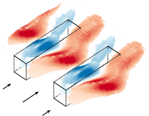
Model domain and three types of farm configurations. (a,b) The farm block configuration (top view and side view). (c,d) The configuration with kelp rows aligned with the current direction. (e, f) The configuration with kelp rows oriented perpendicular to the current direction.

A precursor inflow method is used to simulate the spatially evolving flow in the kelp farm simulations (Churchfield et al. Reference Churchfield, Lee, Michalakes and Moriarty2012; Stevens, Graham & Meneveau Reference Stevens, Graham and Meneveau2014; Yan et al. Reference Yan, McWilliams and Chamecki2021). In this method the turbulent velocity and temperature fields at the upstream boundary of the domain are obtained from a precursor simulation. The precursor simulation is separately conducted with identical conditions without the farm, until the turbulent flow reaches a quasi-equilibrium state. A fringe region (length  $L_{fr}=100\,{\rm m}$) is used at the downstream end of the domain of the farm simulations. In this fringe region the flow field is smoothly forced toward the inflow conditions provided by the precursor simulation at the end of every time step. The precursor inflow method allows the turbulence produced by the precursor simulation to enter the domain of the farm simulations, while permitting the farm wakes to exit without cycling back through the periodic boundary conditions.
2.3. Farm configuration
The cultivation of macroalgae in open ocean environments involves a diverse range of aquaculture structures. A representative farm configuration is considered here and consists of a series of organized longlines spaced horizontally (Yan et al. Reference Yan, McWilliams and Chamecki2021; Frieder et al. Reference Frieder2022). Each longline is anchored at both ends and is also connected to surface buoys. Growth ropes, where kelp is seeded, are attached perpendicular to the longline. Kelp is cultivated at  $h_b=20\,{\rm m}$, i.e. the longline deployment depth, and grows upright due to its buoyancy. The frond surface area density is assumed to be horizontally uniform within each canopy row (each longline set) for simplicity. In the present study, we explore various farm configurations by varying the canopy row spacing and orientation and by comparing different vertical profiles of frond surface area density within the row.
Two vertical profiles of frond surface area density are considered, which represent two different growth stages of kelp (Frieder et al. Reference Frieder2022): (i) an intermediate growth stage with kelp extending from the farm base to around 2 m below the sea surface; (ii) a fully grown stage with kelp extending from the farm base to the sea surface, with notably high frond area density at the top due to a large portion of the fronds floating at the sea surface. The frond surface area density profiles of the two stages are obtained by conversion of the algal biomass (Frieder et al. Reference Frieder2022) and are plotted in figure 2. Harvest practices typically concentrate on the uppermost 1–2 m part of kelp, resulting in the reduction of frond density to zero near the surface. This causes the frond density profile to revert to the earlier growth stage from the fully grown stage. Henceforth, we refer to the earlier growth stage – with a low frond density near the surface – as the ‘harvested’ profile, and the fully grown stage – with a high frond density near the surface – is referred to as the ‘ripe’ profile.
Vertical profiles of frond surface area density  $a$, normalized by the farm base depth $h_b$. The solid line represents the harvested profile, and the dash-dotted line represents the ripe profile. The depth average value $\langle a\rangle _z=1.14\,{\rm m}^{-1}$ ( $\langle a\rangle _z h_b=23$) for the harvested profile, and $\langle a\rangle _z=2.20\,{\rm m}^{-1}$ ( $\langle a\rangle _z h_b=44$) for the ripe profile.

In addition, we examine a variety of kelp row arrangements for each vertical profile of frond area density. The farm parameters for all the simulations are summarized in table 1 in Appendix A. The first set of arrangements (cases ‘S’) has the longlines aligned parallel to the  $x$-direction (the direction of waves and geostrophic flow), extending the length of the farm. The longlines are repeated at a fixed distance $S_{MF}$ in the $y$-direction (figure 1c,d). We conduct a range of farm simulations with varying $S_{MF}$ and kelp row width (growth rope length) $W_{MF}$ (details provided in Appendix A).
The effective frond area density over the farm is defined as
 \begin{equation} \left\langle a \right\rangle_{xyz} = \frac{1}{L_{MF}L_yh_b} \int_0^{L_{MF}} \int_{{-}L_y/2}^{L_y/2}\int_{{-}h_b}^{0} a\, \text{d}\kern0.7pt x\,\text{d} y\,\text{d} z. \end{equation}
The frond area density  $a$ takes the form depicted in figure 2 within the kelp rows and is 0 in the gaps between rows. The effective frond density thus decreases as the spacing between kelp rows increases, while keeping the row width unchanged.
Another set of farm arrangements (cases ‘B’) assumes a scenario where the kelp rows are positioned close enough so that there is no gap in between, i.e. essentially forming a uniform kelp farm block (figure 1a,b). The two profiles in figure 2 are employed in simulations involving this farm block configuration. Additionally, we conduct farm block simulations with varying effective density by introducing a multiplication factor to each frond density profile.
In the third set of farm arrangements (cases ‘PS’), the longlines are rotated by  $90^{\circ }$, so that kelp rows are oriented parallel to the $y$-direction, perpendicular to the geostrophic flow (figure 1e, f). This set of arrangements also includes a range of values of $S_{MF}$ and $W_{MF}$, mirroring the above-mentioned simulations with longlines aligned parallel to the $x$-direction.
Specifically, we have selected three simulations as representatives for an in-depth examination of the turbulence generation mechanisms. These selected cases are S26H (spaced farm rows parallel to the  $x$-direction with a harvested profile, $S_{MF}=26\,{\rm m}$ and $W_{MF}=8\,{\rm m}$; refer to table 1) and B1H and B1R (i.e. farm block simulations with harvested and ripe profiles, respectively). By comparing these three simulations, we aim to elucidate the impacts of cross-stream spacing and the vertical frond area density profile on OML turbulence generation. The effects of effective density and kelp row orientation will be discussed subsequently, following the analysis of turbulence generation mechanisms.
3. Farm hydrodynamics
In this section we present the adjustment of mean flow to the kelp farm as well as the turbulence generated by the farm. We first introduce a flow decomposition to isolate distinct flow components. The instantaneous flow field can be split into the time-averaged and fluctuating components, i.e.
 \begin{equation} \boldsymbol{u}(x,y,z,t) = \bar{\boldsymbol{u}}(x,y,z) + \boldsymbol{u}'(x,y,z,t). \end{equation}
The overline represents the time average, and the prime represents temporal fluctuations about the time average. Further, the time-averaged flow field is decomposed into a cross-stream average and a steady cross-stream deviation
 \begin{equation} \bar{\boldsymbol{u}}(x,y,z) = \left\langle\bar{\boldsymbol{u}}\right\rangle_y(x,z) + \bar{\boldsymbol{u}}^c(x,y,z), \end{equation}
where  $\langle \boldsymbol {\cdot }\rangle _y$ denotes the spatial averaging in the $y$-direction.
The temporal and cross-stream average  $\langle \bar {\boldsymbol {u}}\rangle _y$ is defined as the mean flow. The steady cross-stream deviation $\bar {\boldsymbol {u}}^c$ is referred to as the secondary flow component, representing the stationary circulation structure generated by lateral variations in farm geometry. Note that $\bar {\boldsymbol {u}}^c$ only exists in farm configurations with laterally spaced farm rows and is negligible in the farm block or in kelp rows that are perpendicular to the geostrophic flow (details shown in following sections). The transient fluctuation $\boldsymbol {u}'$ represents the turbulence component.
Similarly, the covariance between velocity and any field  $\phi$ can be decomposed as
 \begin{equation} \left\langle\overline{\boldsymbol{u}\phi}\right\rangle_y = \left\langle\bar{\boldsymbol{u}}\right\rangle_y\left\langle \bar{\phi}\right\rangle_y + \left\langle\bar{\boldsymbol{u}}^c \bar{\phi}^c \right\rangle_y + \left\langle\overline{\boldsymbol{u}'\phi'}\right\rangle_y. \end{equation}
The first term on the right-hand side stands for the contribution from the mean flow; the second term represents the effect of the secondary flow, akin to a dispersive flux (Finnigan Reference Finnigan2000); the third term represents the turbulent flux.
Specifically, we focus on three simulations, S26H, B1H and B1R, as representatives to illustrate the influences of kelp row spacing in the cross-stream direction and the vertical profiles of frond area density. Section 3.1 presents the adjustment of the time-mean flow field in the presence of kelp farms. Section 3.2 provides an overview of the hydrodynamic characteristics of all the different farm configurations. Section 3.3 compares the Langmuir circulation patterns across the three representative cases. Subsequently, we quantify turbulence and steady secondary flows in the three cases in § 3.4, and calculate the vertical velocity skewness in § 3.5 to characterize the turbulence generated by the farm.
3.1. Mean flow
The mean flow structure is substantially altered by the presence of kelp farms. Figure 3 shows the adjustment of mean flow in case S26H (spaced rows aligned with the  $x$-direction) as an example. As flow enters the canopy region, the streamwise velocity decreases due to the drag force exerted by the kelp (figure 3a). A shear layer develops beneath the farm as a result of discontinuity in kelp frond density. In addition, vertical shear is also increased within the canopy due to the vertical variability of frond area density (figure 2). The shear within the farm is most pronounced near the leading edge, and gradually diminishes downstream as turbulence generated in the farm leads to vertical mixing of momentum.
Side views of mean flow in case S26H (spaced rows aligned with the current, harvested profile). (a) Normalized streamwise velocity  $\langle \bar {u}\rangle _y/u_g$. (b) Normalized vertical velocity $\langle \bar {w}\rangle _y/u_*$. The mean flow is averaged in time and in the cross-stream direction. Dotted rectangles show the extent of the farm, and the solid grey line in (b) represents the mixed layer depth. Note that $\langle \bar {u}\rangle _y$ is normalized by $u_g$ and $\langle \bar {w}\rangle _y$ is normalized by $u_*$, and $\langle \bar {u}\rangle _y$ is generally much larger than $\langle \bar {w}\rangle _y$.

At the canopy leading edge, as the streamwise flow is decelerated by the pressure gradient set up by the canopy drag, the mean downward vertical velocity develops as a result of mass conservation (figure 3b). Likewise, the pressure decrease at the trailing edge induces an upward velocity in the farm's wake region. Note that a fringe region is located between the wake region and the downstream end of the domain (not shown), where the flow field is forced toward the precursor inflow conditions to avoid the wake effect on periodic horizontal boundary conditions. The farm-induced mean flow adjustment in case S26H closely aligns with the previous study by Yan et al. (Reference Yan, McWilliams and Chamecki2021); other cases involving different farm configurations will be explored further.
We define the mixed layer depth (MLD)  $z_i$ as the depth at which the laterally averaged potential temperature $\langle \bar {\theta }\rangle _y$ first deviates from its surface value by $\Delta \theta$ (e.g. Kara, Rochford & Hurlburt Reference Kara, Rochford and Hurlburt2000), here using $\Delta \theta = 0.01\,{\rm K}$. The MLD is around 25 m at the upstream boundary where the inflow originates. The mixed layer deepens to nearly 40 m due to the downwelling created by the farm, which then recovers downstream from the farm. The farm is always situated above the pycnocline, and the buoyancy effect is thus considered to have negligible influence on turbulence generation within the farm.
The canopy drag length  $L_c$ is defined as (Belcher et al. Reference Belcher, Jerram and Hunt2003; Rominger & Nepf Reference Rominger and Nepf2011; Belcher, Harman & Finnigan Reference Belcher, Harman and Finnigan2012)
 \begin{equation} L_c = \frac{2}{C_D \left\langle a\right\rangle_{xyz}}, \end{equation}
where  $C_D$ is the drag coefficient, and $\langle a\rangle _{xyz}$ is the effective frond density in (2.6). The factor of 2 in (3.4) accounts for the projection of frond surface area, as denoted by the term $\boldsymbol {P}$ in (2.5). The canopy drag length is $L_c=347\,{\rm m}$ for case S26H. Note that $L_c$ varies with the effective density and thus the farm configuration, and case B1R (farm block, ripe profile) has the smallest $L_c$ of 61 m. The length of the adjustment region scales in proportion to $L_c$, typically by a factor of $4.5\unicode{x2013}6$ (Belcher et al. Reference Belcher, Harman and Finnigan2012). Therefore, the adjustment region length for the farm configurations in this study is either comparable to or larger than the farm length, suggesting that the canopy flow does not reach a fully developed state prior to exiting the farm. This explains the streamwise variations found in the mean flow field within the farm (figure 3) and also agrees with the analysis of the turbulence field presented in the following sections.
The mean flow properties in the other simulations B1H and B1R are compared with S26H (figure 4). The vertical profiles in figure 4 are averaged in the cross-stream direction, and also averaged in the streamwise direction from the leading edge to  $5h_b$ into the farm, a distance comparable to the canopy drag length $L_c$ in cases B1H and B1R. Generally cases B1H and B1R are similar to case S26H shown above, except that B1H and B1R demonstrate more pronounced downwelling at the leading edge and stronger vertical shear below the canopy, due to their higher effective frond area density and greater drag. In addition, the vertical shear of the mean streamwise flow within the farm is also stronger in B1H compared with S26H, because of the higher effective density in B1H. Moreover, while the streamwise mean velocity monotonically increases from the canopy bottom to the sea surface in cases S26H and B1H, the vertical shear reverses near the surface in B1R, because the presence of the uppermost dense layer in B1R locally enhances drag and decelerates flow.
Vertical profiles of streamwise velocity  $\langle \bar {u}\rangle _{y}$ (a) and vertical velocity $\langle \bar {w}\rangle _{y}$ (b). The velocities are time averaged and cross-stream averaged, at $x/h_b=2.5$. Note that the geostrophic current $u_g=0.2\,{\rm m}\,{\rm s}^{-1}$ has been subtracted in (a). The streamwise velocity in (a) is normalized by $u_g$, and the vertical velocity in (b) is normalized by the friction velocity $u_*=0.0061\,{\rm m}\,{\rm s}^{-1}$. Black lines represent case S26H, spaced rows aligned with the geostrophic current, with the harvested profile; red lines represent case B1H, farm block with the harvested profile; blue lines represent case B1R, farm block with the ripe profile. Additionally, the dash-dotted line in (a) shows the streamwise velocity profile at the upstream boundary (inflow condition at $x/h_b=-7.5$). The dashed line in (a) represents the vertical profile of Stokes drift $u_s$. The dotted horizontal lines mark the farm bottom, and the thin solid horizontal lines represent the inflow MLD.

Note that the selected cases have a relatively high effective density  $\langle a\rangle _{xyz}$. Other simulations that are not presented here, e.g. with larger spacing between kelp rows or with a lower frond area density, generally have weaker downwelling at the farm leading edge and weaker shear in the mean streamwise flow.
3.2. Overview
Along with modifications to the mean flow, the presence of the farm also affects Langmuir circulation patterns and turbulence intensity. In this section, we present an overview of the distinct flow patterns associated with various farm configurations, before moving on to detailed analysis of Langmuir circulation and turbulence. The magnitudes of mean flow, secondary flow and turbulence components within and below the canopy are summarized in figure 5 for all the farm configurations in table 1.
Mean flow ( $\bar {u}$, $\bar {w}$, and shear $\partial \bar {u}/\partial z$), secondary flow ( $\bar {w}^c$) and turbulence ( $w'$) statistics within the farm (a–c) and below the farm (d–f). Each point represents a simulation (see the legends for details). Note that row $0^\circ$ and row $90^\circ$ denote kelp rows aligned with and perpendicular to the current, respectively. The horizontal dashed line in (a) represents the intensity of standard Langmuir turbulence in the absence of a farm. The thick grey lines in (a) are fitting curves for the three types of farm configurations. Averaging within the farm is conducted between $z=0$ and $-h_b$, and averaging below the farm is between $-h_b$ and $-2h_b$. The horizontal axis in (a,c–f) is the effective density $\langle a \rangle _{xyz}$ averaged within the farm. Note that the shear and vertical velocity are negative below the farm in (e, f). The mean streamwise velocity is normalized by the geostrophic velocity $u_g=0.2\,{\rm m}\,{\rm s}^{-1}$, the mean vertical velocity is normalized by the friction velocity $u_*=0.0061\,{\rm m}\,{\rm s}^{-1}$ and the variance terms are normalized by $u_*^2$.

The mean streamwise flow within the farm decreases with the increased effective density  $\langle a \rangle _{xyz}$ due to the greater kelp drag (figure 5c), leading to stronger downwelling below the farm as a result of mass conservation (figure 5f). In the shear layer below the canopy, the vertical shear of streamwise mean flow generally increases in magnitude with the increased effective frond density (figure 5e). Correspondingly, the turbulence intensity in the shear layer – quantified by the variance of the temporal fluctuating component of vertical velocity $\langle \overline {w'w'} \rangle _{xyz}$ – increases with the increased $\langle a \rangle _{xyz}$ (figure 5d). This is consistent with that expected for classical canopy flow, where the canopy effect positively depends on $\langle a \rangle _{xyz}$ (e.g. Poggi et al. Reference Poggi, Porporato, Ridolfi, Albertson and Katul2004; Bailey & Stoll Reference Bailey and Stoll2013). For shear layer statistics, the average is calculated within a vertical distance equal to $h_b$ beneath the canopy bottom, i.e.
 \begin{equation} \left\langle
\boldsymbol{\cdot} \right\rangle_{xyz} =
\frac{1}{L_{MF}L_yh_b} \int_0^{L_{MF}}
\int_{{-}L_y/2}^{L_y/2}\int_{{-}2h_b}^{{-}h_b}
\,\boldsymbol{\cdot}\, \text{d}\kern0.7pt x\,\text{d}
y\,\text{d} z,
\end{equation}
\begin{equation} \left\langle
\boldsymbol{\cdot} \right\rangle_{xyz} =
\frac{1}{L_{MF}L_yh_b} \int_0^{L_{MF}}
\int_{{-}L_y/2}^{L_y/2}\int_{{-}2h_b}^{{-}h_b}
\,\boldsymbol{\cdot}\, \text{d}\kern0.7pt x\,\text{d}
y\,\text{d} z,
\end{equation}
for averaging below the farm. Here, we select the vertical component  $w'$ because of its direct relevance to vertical transport in kelp farms. More discussions about the other components $u'$ and $v'$ and turbulence anisotropy will be presented later. Note that the scatter in figure 5(d,e) primarily results from the two different vertical profiles of frond area density. The dense layer near the surface in the ripe profile has a small influence on the shear layer dynamics below the canopy, and excluding this dense surface layer from the effective density calculation can lead to improved alignment in figure 5(d,e).
As a contrast to the shear layer turbulence generated below the canopy, turbulence intensity within the farm displays a more complex dependence on the effective frond density (figure 5a). Note that, within this depth range, e.g. between the sea surface and  $z=-h_b$, standard Langmuir turbulence is expected to occur in the absence of the canopy (McWilliams et al. Reference McWilliams, Sullivan and Moeng1997). In the presence of the canopy, for kelp frond density with the harvested vertical profile, $\langle \overline {w'w'} \rangle _{y}$ is enhanced compared with that of the standard Langmuir turbulence. Moreover, the intensity of enhanced turbulence within the farm positively depends on the effective density $\langle a \rangle _{xyz}$. However, for farm configurations with the ripe vertical profile, turbulence is inhibited in farm blocks and kelp rows that are perpendicular to the geostrophic current. For farms with kelp rows aligned with the current, $\langle \overline {w'w'}\rangle _{y}$ is enhanced compared with the standard Langmuir turbulence only for cases with an intermediate effective density $\langle a \rangle _{xyz}$. This enhancement diminishes as $\langle a \rangle _{xyz}$ increases, i.e. with closely spaced rows that asymptotically resemble a farm block, or, as $\langle a \rangle _{xyz}$ decreases, asymptoting toward a scenario without a farm.
For canopy flow without the influence of waves and Langmuir circulation, the turbulence intensity within the canopy is usually anticipated to decrease with increased effective density, due to the weaker penetration of shear layer eddies (Poggi et al. Reference Poggi, Porporato, Ridolfi, Albertson and Katul2004; Bailey & Stoll Reference Bailey and Stoll2013). Nevertheless, our simulations show that the turbulence intensity in the farm either positively depends on the effective density or exhibits a more complex dependence. This contrasting dependence on effective density underscores the distinct type of turbulence that arises from the interaction between the canopy and the OML, which is called the farm-generated Langmuir turbulence and will be presented in the following sections.
Moreover, secondary flow  $\langle \bar {w}^c\bar {w}^c \rangle _{y}$ (stationary circulation) can be generated within the farm exclusively in cases with kelp rows aligned with the current (figure 5b). The occurrence of stationary secondary circulation associated with spaced kelp rows is consistent with the previous study by Yan et al. (Reference Yan, McWilliams and Chamecki2021), who referred to these flow patterns as ‘attached Langmuir circulation’. The intensity of $\langle \bar {w}^c\bar {w}^c \rangle _{y}$ is always stronger in cases with the harvested profile compared with the ripe profile. Our simulations do not allow for a clear identification of the maximum intensity with respect to the lateral spacing $S_{MF}$, and the peak of $\langle \bar {w}^c\bar {w}^c \rangle _{y}$ appears to fall within the range of $S_{MF}=52\,{\rm m}$ and 208 m. Note that secondary flow never occurs in the shear layer below the canopy.
Overall, these various flow statistics highlight the distinction between the hydrodynamics within the farm (within the OML where Langmuir turbulence is expected) and the classical shear layer turbulence beneath the farm. In addition, the contrast between different farm simulations suggests that these hydrodynamic processes depend on both the vertical frond density profile and horizontal farm arrangement, and these factors will be analysed in detail below.
3.3. Langmuir circulations
Three representative simulations are selected to investigate the distinct flow patterns associated with different farm configurations, i.e. case S26H (spaced rows aligned with the  $x$-direction, harvested profile), case B1H (farm block, harvested profile) and case B1R (farm block, ripe profile). Snapshots of instantaneous vertical velocities of the three simulations are compared in figure 6, on a horizontal plane at $z=-0.25h_b$.
Snapshots of normalized vertical velocity  $w/u_*$ on a horizontal plane at $z=-0.25h_b$, for cases S26H (a), B1H (b) and B1R (c). Dotted rectangles show the extent of the farm block or rows.

Upstream of the farm, the elongated streaks of downward vertical velocity are indicative of standard Langmuir circulation (e.g. McWilliams et al. Reference McWilliams, Sullivan and Moeng1997). These patterns are typically featured by stronger downward motions within narrower regions compared with the broader and weaker upward motions. In addition, the streaks are generally rotated to the right of the direction of the wind and waves ( $x$-direction) as a result of Coriolis. The standard Langmuir circulation patterns are transient, characterized by their continuous cycles of formation, evolution and dissipation.
For the case with laterally spaced kelp rows (case S26H), Langmuir circulation within the farm area shows a notable increase in magnitude compared with the standard Langmuir circulation in the upstream region (figure 6a). Moreover, these Langmuir circulation patterns are locked in space in the cross-stream direction, generally with upward motions within the kelp rows and downward motions within the gaps in between. The Langmuir patterns in the farm are generally stationary in time, although the smaller-scale coherent structures are still transient. These patterns are termed as the ‘attached Langmuir circulation’ (Yan et al. Reference Yan, McWilliams and Chamecki2021) because of their locked-in-space characteristics.
For the farm block case with the harvested profile (case B1H), Langmuir circulation is also enhanced within the farm compared with the upstream region (figure 6b). However, these farm-enhanced Langmuir circulation patterns are completely transient and not locked in space due to the absence of repeated kelp rows, and we thus refer to these patterns as ‘unattached Langmuir circulation’. In the vertical direction, both the attached and unattached Langmuir circulation patterns have comparable dimensions to the farm height, with their maximum intensity found at a depth of around 10 m (quantitative results shown in § 3.4).
Furthermore, in contrast to the Langmuir patterns found in case B1H, Langmuir circulation notably vanishes in the farm in case B1R (farm block with the ripe profile, see figure 6c). This implies an absence of the Langmuir circulation generation mechanism or an increase in dissipation in case B1R, as will be investigated below. It is also worthwhile noting that the vertical velocity exhibits patterns aligned with the lateral direction in case B1R, in contrast to the streaks aligned with the streamwise direction in other cases. These distinct patterns in case B1R (e.g. for  $x/h_b$ from 5 to 10) correspond to shear-generated turbulence within the farm, as the canopy drag force significantly decelerates flow near the sea surface and enhances the vertical shear (figure 4a). Moreover, shear layer turbulence generated at the farm bottom edge could penetrate into the farm in cases where Langmuir turbulence is inhibited (e.g. for $x/h_b>15$ in figure 6c). The distinct Langmuir patterns as well as the penetration of shear layer eddies will be further analysed in subsequent sections.
Additionally, a simulation with laterally spaced kelp rows with the ripe profile (case S26R) is examined. In this case, attached Langmuir circulation is generated in the farm (not shown) that resembles the patterns found in case S26H, while the magnitude of vertical velocity is smaller in case S26R compared with S26H.
3.4. Langmuir turbulence and bottom shear layer turbulence
The temporally and laterally averaged vertical velocity variance associated with transient eddies ( $\langle \overline {w'w'}\rangle _{y}$) is calculated to quantify the farm-generated turbulence (figure 7). The vertical component $w'$ is selected because Langmuir turbulence is usually characterized by its large vertical velocity variance (McWilliams et al. Reference McWilliams, Sullivan and Moeng1997; Yan et al. Reference Yan, McWilliams and Chamecki2021), and the vertical component also directly influences vertical transport.
Side views of the transient component of vertical velocity variance  $\langle \overline {w'w'}\rangle _{y}/u_*^2$ for cases S26H (a), B1H (b) and B1R (c). The results are temporally and laterally averaged. Dotted rectangles show the extent of the farm.

Standard Langmuir turbulence occurs upstream of the farm, with the maximum  $\langle \overline {w'w'}\rangle _{y}$ found slightly below the sea surface, e.g. around 5–10 m, consistent with McWilliams et al. (Reference McWilliams, Sullivan and Moeng1997). Within the farm, similar Langmuir-type turbulence is generated in the two cases with the harvested profile (B1H and S26H, figure 7a,b). The farm-generated Langmuir turbulence has a stronger magnitude compared with the standard Langmuir turbulence in the upstream region, while its vertical variance $\langle \overline {w'w'}\rangle _{y}$ also peaks at a similar depth of around 5–10 m. In the streamwise direction, the intensity of farm-generated Langmuir turbulence increases from the leading edge of the farm as flow adjusts to the canopy drag, with a maximum at around $x/h_b=10$ (also see figure 9). Turbulence intensity then decreases toward the farm trailing edge, due to the decrease in the production mechanisms and the damping by kelp drag and viscosity (details examined in the energy budget calculation in § 4). In addition, the farm-generated Langmuir turbulence is stronger in the farm block case B1H than the spaced rows case S26H (both with a harvested profile), and this aligns with the positive dependence on effective frond area density in figure 5(a). By contrast, no intensified turbulence is found in the farm block with a ripe profile (case B1R) (figure 7c), consistent with the absence of Langmuir patterns in the map view plot of vertical velocity (figure 6c).
The intensified turbulence in the kelp farm is referred to as Langmuir type because its generation relates to the Stokes drift (see § 4), akin to the standard Langmuir turbulence. Furthermore, the intensified Langmuir-type turbulence in the farm completely disappears in another set of test cases (S26H-NW, B1H-NW, B1R-NW, not presented here), where the surface wave forcing is excluded. This provides corroborating evidence that the Langmuir-type turbulence results from the interaction between waves and canopy flow.
In addition to the Langmuir-type turbulence generated within the farm, shear layer turbulence occurs at the bottom edge of the canopy. The shear layer turbulence, as a characteristic of classical canopy flow, is consistently found across all the simulations regardless of the presence or absence of Langmuir-type turbulence within the farm. The intensity of shear layer turbulence typically increases with the increased effective density (e.g. Bailey & Stoll Reference Bailey and Stoll2013), so that the farm block cases (B1H and B1R) exhibit stronger turbulence below the farm compared with the case with spaced kelp rows (S26H).
While the shear layer turbulence mostly occurs beneath the canopy, it also penetrates into the canopy, in particular in the downstream part of the farm. Nevertheless, the penetrated shear layer turbulence is overall much weaker than the farm-generated Langmuir turbulence (as will be substantiated by the skewness analysis in § refsec:results-skewness). Therefore, in cases with enhanced Langmuir turbulence, shear layer turbulence has a minimal influence on the turbulence statistics calculated within the farm. This point is also supported by the dependence of turbulence intensity on the effective density  $\langle a \rangle _{xyz}$ in figure 5(a). Turbulence intensity within the canopy is expected to decrease with increased $\langle a \rangle _{xyz}$, assuming penetration of shear layer is the dominant source of turbulence (Poggi et al. Reference Poggi, Porporato, Ridolfi, Albertson and Katul2004; Bailey & Stoll Reference Bailey and Stoll2013). Nevertheless, our simulations show a more complex dependence of turbulence intensity on $\langle a \rangle _{xyz}$, due to the dominance of Langmuir-type turbulence within the farm.
We have primarily focused on the vertical component  $w'$, and the horizontal components $u'$ and $v'$ generally display similar distributions to $w'$. However, it is worthwhile noting that the transient eddies are not isotropic, and this turbulence anisotropy also provides insights into distinguishing between different types of farm-generated turbulence. The shear layer turbulence typically has a stronger streamwise component $u'$ compared with the other components, while the Langmuir-type turbulence features a relatively stronger vertical component $w'$.
$w'$.
In figure 8, we plot the temporally and laterally averaged vertical velocity variance associated with the steady secondary flow, denoted as  $\langle \bar {w}^c\bar {w}^c\rangle _{y}$. Note that secondary flow includes both the lateral variations in streamwise velocity ( $\bar {u}^c$) and the stationary lateral circulation ( $\bar {v}^c$ and $\bar {w}^c$). Secondary flow exclusively occurs in the case with laterally spaced kelp rows (case S26H), where attached Langmuir circulation occurs. In farm block simulations where transient Langmuir circulation has been found, $\langle \bar {w}^c\bar {w}^c\rangle _{y}$ is generally negligible. The region of high $\langle \bar {w}^c\bar {w}^c\rangle _{y}$ roughly coincides with that of high $\langle \overline {w'w'}\rangle _{y}$ for case S26H, while the peak of $\langle \bar {w}^c\bar {w}^c \rangle _{y}$ is slightly upstream of $\langle \overline {w'w'} \rangle _{y}$ (figure 9).
Side view of the secondary flow component of vertical velocity variance  $\langle \bar {w}^c \bar {w}^c\rangle _{y}/u_*^2$ for cases S26H. The results are temporally and laterally averaged. The dotted rectangle shows the extent of the farm.

Streamwise variations of  $\langle \overline {w'w'}\rangle _{y}/u_*^2$ (dashed lines) and $\langle \bar {w}^c \bar {w}^c\rangle _{y}/u_*^2$ (solid lines) for cases S26H (black), B1H (red) and B1R (blue). The results are temporally, laterally and vertically ( $z=0$ to $-h_b$) averaged. Vertical dotted lines show the extent of the farm.

We calculated the lateral-direction wavenumber spectra of the vertical velocity to investigate the characteristic lateral spacing of Langmuir circulations. In case S26H (rows with a spacing of 26 m), the spectral peak in the farm aligns with the lateral row spacing  $S_{MF}=26\,{\rm m}$ (figure 10a). Similarly, for case S52H with rows spaced at 52 m, the peak wavelength corresponds to $S_{MF}=52$ m. Note that these spectra are calculated from the total vertical velocity $w$, and the energy peaks in the above two cases are predominantly contributed by the secondary flow component $\bar {w}^c$. The peaks would be considerably less distinct if calculating the spectra using the turbulent component $w'$ alone. In case B1H (farm block with the harvested profile), the spectral peak corresponds to a wavelength of around 30 m (figure 10b). This peak wavelength is slightly smaller than that of the inflow condition with standard Langmuir turbulence. In contrast to the spaced rows, the farm block exhibits a less distinct peak, due to the absence of secondary flow structures caused by row spacing. For case B1R (farm block with the ripe profile), the spectrum exhibits no apparent peak because of the inhibition of Langmuir turbulence in the farm, with a weakened overall magnitude compared with that upstream of the farm.
Spectra of the vertical velocity vs the lateral-direction wavenumber  $k_y$. (a) Cases S26H (rows aligned with the $x$-direction, 26 m spacing, solid black line) and S52H (52 m spacing, solid yellow line), at $x/h_b=10$ and averaged between $z=0$ and $z=-h_b$. The dash-dotted black line represents the inflow condition at the upstream boundary ( $x/h_b=-7.5$). Two vertical grey lines indicate the corresponding spacing between kelp rows, 26 and 52 m, respectively. (b) Cases B1H (solid blue line) and B1R (solid red line).

3.5. Vertical velocity skewness
The skewness of the vertical turbulence component, defined as  $\langle \overline {{w'}^3} \rangle _y/\langle \overline {{w'}^2} \rangle _y^{3/2}$, is plotted in figure 11 to illustrate the distinct attributes of various types of turbulence. The standard Langmuir turbulence in the upstream region is characterized by its negative skewness of vertical velocity (McWilliams et al. Reference McWilliams, Sullivan and Moeng1997). The negative skewness indicates stronger downward motions confined within narrower regions in comparison with broader and weaker upward motions, consistent with the Langmuir circulation patterns shown in figure 6.
Side views of the skewness of  $w'$ (transient component of vertical velocity) for cases S26H (a), B1H (b) and B1R (c). The results are temporally and laterally averaged. Dotted rectangles show the extent of the farm.

In the shear layer generated at the canopy bottom, the vertical velocity skewness is generally negative beneath the canopy and positive near the canopy edge (figure 11). The positive skewness of vertical velocity near the canopy edge indicates the dominance of sweep events that bring high-momentum fluid into the canopy, consistent with those found in classical canopy flow without waves (Raupach & Thom Reference Raupach and Thom1981; Katul et al. Reference Katul, Kuhn, Schieldge and Hsieh1997; Poggi et al. Reference Poggi, Porporato, Ridolfi, Albertson and Katul2004). Note that the skewness sign in the suspended canopy is opposite to that of submerged benthic canopies due to the reversed geometry of the problem set-ups (i.e. here sweep events are characterized by intensified positive vertical velocities into the canopy). Conversely, the negative skewness of vertical velocity below the canopy is indicative of the prevalence of ejection events.
The vertical velocity skewness of the farm-generated Langmuir turbulence appears less clear, displaying mostly negative values. However, the boundary between shear layer turbulence and farm-generated Langmuir turbulence remains discernible through their difference in the skewness sign inside the canopy. Specifically, in case B1H in figure 11(b), the positive vertical velocity skewness associated with shear layer turbulence occupies less than one third of the canopy height. Furthermore, the region with the highest turbulence intensity is located above the region with positive skewness (figure 7b), underscoring that the majority of energy within the farm is attributed to Langmuir-type turbulence rather than the penetrated shear layer turbulence.
For case B1R (farm block with the ripe profile), the concept of skewness within the farm lacks significance due to the absence of Langmuir-type turbulence. However, indications of shear-generated turbulence can be found within the farm, e.g. in the range of  $x/h_b$ from 0 to 5, where the mean flow is adjusting to the canopy drag (figure 11c). This shear-generated turbulence within the farm exhibits similar characteristics to the shear layer turbulence below the canopy bottom edge, although with lower intensity. It results from the vertical variability in frond area density, and then rapidly dissipates downstream in the farm.
Similarly, we define a skewness for the steady secondary flow as  $\langle {{\bar w}^c3}\rangle _y/\langle {{\bar w}^c2}\rangle _y^{3/2}$. The steady secondary velocity is generally upward in the kelp rows and downward in the gaps between kelp rows (figure 6). In cases where the kelp rows are narrower than the gaps, e.g. case S26H in figure 12, the upward secondary flow is typically stronger in magnitude than the downward flow as a result of mass balance. Therefore, a positive skewness of the steady secondary vertical velocity is evident in the upstream part of the farm (figure 12). Toward the downstream region of the farm, the vertical secondary velocity skewness becomes less distinct. This can be attributed to the lateral expansion of Langmuir wakes linked to kelp rows, so that regions of upwelling may extend beyond the constraints of kelp rows (figure 6a, also see Appendix B for a clearer presentation of the Langmuir wake pattern in case S208H, the single-row simulation). As one may anticipate, the skewness of secondary flow varies with changes in farm width and lateral spacing across different farm configurations. As an example, the skewness $\langle {{\bar w}^c3}\rangle _y/\langle {{\bar w}^c2}\rangle _y^{3/2}$ in case S208H can reach up to a value of 3, where the upwelling of secondary flow is confined within a single kelp row before wake expansion occurs.
Side view of the skewness of  $\bar {w}^c$ (steady secondary flow component of vertical velocity) for case S26H. The results are temporally and laterally averaged. The dotted rectangle shows the extent of the farm.

The skewness of turbulence and secondary flow investigated above also influences diffusive and dispersive fluxes in the farm, potentially leading to asymmetric vertical nutrient transport (Wyngaard & Brost Reference Wyngaard and Brost1984; Wyngaard & Weil Reference Wyngaard and Weil1991; Chor, McWilliams & Chamecki Reference Chor, McWilliams and Chamecki2020, Reference Chor, McWilliams and Chamecki2021). Note that spurious oscillations displaying alternating positive and negative skewness can be found in the secondary flow and turbulence components, e.g. around  $z/h_b=-2$ and $x/h_b=15$ in figure 12 and around $z/h_b=-2$ and $x/h_b=20$ in figure 11(a). These oscillations occur in regions where $\bar {w}^c$ or $w'$ is minimal and thus do not have practical significance.
4. Kinetic energy balance
In this section we investigate the kinetic energy equations to understand the sources of Langmuir circulation and turbulence. Following the convention in (3.2) and (3.3), we decompose the total kinetic energy  $K_T$ into the mean flow energy $K_M$, secondary flow energy $K_{SE}$ and turbulence kinetic energy $K_{TE}$, i.e.
 \begin{equation} K_T = \frac{1}{2}\left\langle \overline{u_i u_i}\right\rangle_y = \underbrace{\frac{1}{2}\left\langle \overline{u_i}\right\rangle_y \left\langle\overline{u_i}\right\rangle_y \vphantom{\frac{1}{2}\left\langle \overline{u'_i u'_i}\right\rangle_y} }_{K_M} + \underbrace{\frac{1}{2}\left\langle \overline{u_i}^c \overline{u_i}^c \right\rangle_y \vphantom{\frac{1}{2}\left\langle \overline{u'_i u'_i}\right\rangle_y} }_{K_{SE}} + \underbrace{\frac{1}{2}\left\langle \overline{u'_i u'_i} \right\rangle_y}_{K_{TE}}. \end{equation}
We can derive the transport equations for  $K_M$, $K_{SE}$ and $K_{TE}$ from the governing equations (2.1) and (2.2) (Yan et al. Reference Yan, McWilliams and Chamecki2021)
 $$\begin{gather} \frac{\text{D}K_M}{\text{D}t} ={-} C_{M-SE} - C_{M-TE} + S_M + D_M + T_M + R_M, \end{gather}$$
 $$\begin{gather}\frac{\text{D}K_{SE}}{\text{D}t} = C_{M-SE} - C_{SE-TE} + S_{SE} + D_{SE} + T_{SE}, \end{gather}$$
 $$\begin{gather}\frac{\text{D}K_{TE}}{\text{D}t} = C_{M-TE} + C_{SE-TE} + S_{TE} + \epsilon_{TE} + D_{TE} + T_{TE}. \end{gather}$$
Here, the material derivative is  $\text {D}/\text {D}t = \partial /\partial t + \langle \overline {u_j}\rangle _y\partial /\partial x_j + u_s\partial /\partial x$. Note that we have neglected the buoyancy production terms, as the farm is located within the OML. Terms $C_{M-SE}$, $C_{M-TE}$ and $C_{SE-TE}$ represent the energy conversion between the mean flow $K_M$, secondary flow $K_{SE}$ and turbulence $K_{TE}$ (also referred to as shear production), written as
 $$\begin{gather} C_{M-SE} ={-} \left\langle \overline{u_i}^c \overline{u_j}^c\right\rangle_y \frac{\partial{\left\langle\overline{u_i}\right\rangle_y}}{\partial{x_j}}, \end{gather}$$
 $$\begin{gather}C_{M-TE} ={-} \left\langle \overline{u_i' u_j'}\right\rangle_y \frac{\partial{\left\langle\overline{u_i}\right\rangle_y}}{\partial{x_j}}, \end{gather}$$
 $$\begin{gather}C_{SE-TE} ={-} \left\langle \overline{u_i' u_j'} \frac{\partial{\overline{u_i}^c}}{\partial{x_j}}\right\rangle_y. \end{gather}$$
Terms  $S_{M}$, $S_{SE}$ and $S_{TE}$ stand for Stokes production that transfers energy between waves and the three flow components, and are given by
 \begin{equation} S_{M} ={-} \left\langle \bar{u}\right\rangle_y \left\langle \bar{w}\right\rangle_y \frac{\partial{u_s}}{\partial{z}}, \quad S_{SE} ={-} \left\langle \bar{u}^c \bar{w}^c \right\rangle_y \frac{\partial{u_s}}{\partial{z}}, \quad S_{TE} ={-} \left\langle \overline{u'w'} \right\rangle_y \frac{\partial{u_s}}{\partial{z}}. \end{equation}
The SGS dissipation term is
 \begin{equation} \epsilon_{TE} ={-}\left\langle \overline{\tau'_{ij} \frac{\partial{u'_i}}{\partial{x_j}}}\right\rangle_y. \end{equation}
The majority of energy dissipation is expected to occur in the small-scale transient eddies for turbulent flows with a large Reynolds number (e.g. Pope Reference Pope2000). Therefore, the energy loss of the larger-scale mean flow and secondary flow due to direct SGS dissipation is considered negligible, and we only focus on the dissipation of turbulence kinetic energy. The canopy drag dissipation terms are
 \begin{equation} D_{M} ={-}\left\langle\overline{u_i}\right\rangle_y \left\langle\overline{F_{D,i}}\right\rangle_y, \quad D_{SE} ={-}\left\langle \overline{u_i}^c \overline{F_{D,i}}^c\right\rangle_y, \quad D_{TE} ={-}\left\langle \overline{u'_{i} F'_{D,i}}\right\rangle_y, \end{equation}
which represent the energy loss or gain associated with canopy drag. In addition, several flux terms representing kinetic energy transport associated with the resolved stress, SGS stress and pressure are collected into the transport terms  $T_M$, $T_{SE}$ and $T_{TE}$. The last term $R_M= f \langle \bar {v}\rangle _y (u_g-u_s)$ in the mean flow energy budget represents the energy transfer between the mean flow, surface waves and the background geostrophic current, resembling the concept of Stokes–Coriolis work (Suzuki & Fox-Kemper Reference Suzuki and Fox-Kemper2016; Yan et al. Reference Yan, McWilliams and Chamecki2021).
We calculate the turbulent kinetic energy budget for case B1H (farm block with the harvested profile), and the major source and sink terms are shown in figure 13. The Stokes production is the dominant source of turbulence upstream of the farm, where standard Langmuir turbulence is found. This agrees with the widely recognized mechanism wherein the generation of Langmuir circulation results from vorticity tilting by the Stokes drift (Craik Reference Craik1977; Leibovich Reference Leibovich1977, Reference Leibovich1983). Within the farm, the Stokes production becomes significantly stronger, which, together with the shear production, contributes to the enhanced Langmuir-type turbulence (figures 13 and 7). Below the farm, shear production provides the dominant source of shear layer turbulence, and Stokes production is weak because the Stokes drift diminishes at greater depth. Both dissipation and canopy drag dissipation terms tend to destroy the turbulence generated within the farm, while in the shear layer below the canopy, the dissipation term is the only sink of turbulence kinetic energy. Note that the secondary flow energy is negligible in the farm block, and there is no energy conversion associated with secondary flow.
Side views of terms in the  $K_{TE}$ budget in (4.2c) for case B1H (farm block, harvested profile). The results are temporally and laterally averaged. Dotted rectangles show the extent of the farm.

In case B1R (farm block with the ripe profile), the shear production term is the major source of turbulence kinetic energy in the shear layer below the canopy (figure 14), consistent with case B1H discussed above (farm block with the harvested profile). However, when focusing within the farm, both the Stokes production and shear production diminish due to the presence of a dense layer near the surface (characteristic of the ripe profile). This explains the absence of Langmuir-type turbulence in figure 7(c). In particular, negative values of Stokes production are even found near the sea surface, indicating that the shear of the Stokes drift velocity contributes to disrupting vortex formation rather than stretching vortex tubes (detailed mechanisms are explained in § 5). Negative vertical shear of the Eulerian velocity arises due to the presence of a dense kelp layer near the surface, which dominates over the positive vertical shear of the Stokes drift (figure 4). This results in a negative sign for the Reynolds stress  $\overline {u'w'}$, and consequently, the Stokes production term acts as a sink for turbulence kinetic energy. The dissipation and kelp drag dissipation terms are not shown for case B1R. The distribution of dissipation generally correlates with that of turbulence intensity, and strong kelp drag dissipation occurs where areas with high kelp frond density intersect with intense turbulence.
Side views of terms in the  $K_{TE}$ budget in (4.2c) for case B1R (farm block, ripe profile). The results are temporally and laterally averaged. Dotted rectangles show the extent of the farm. Note that differences between case B1R and case B1H (figure 13) primarily lie in the energy production mechanisms. The dissipation and canopy drag dissipation terms are not shown here because the energy loss mechanisms in case B1R are similar to case B1H.

It is worthwhile noting that the originally farm-generated vertical shear has a comparable magnitude in cases B1R and B1H, e.g. near the farm leading edge in the range of  $x/h_b$ between 0 and 5 (figure 4). In fact, case B1R has even more pronounced sheared flow near the surface due to the existence of the dense layer. Nonetheless, the rapid downstream increase in shear production in case B1H compared with B1R, e.g. for $x/h_b$ from 5 to 15, indicates that its strength does not solely depend on the vertical shear induced by variations in frond area density. Instead, the increased Stokes production in case B1H plays a critical role in initiating the growth of turbulence and thus contributing to the enhancement of shear production. Further investigation of the distinct Stokes mechanisms in the two cases will be presented in § 5.
The turbulence kinetic energy budget is also evaluated for the case with laterally spaced rows (S26H, harvested profile). The distributions of Stokes production (figure 15), dissipation and canopy drag dissipation (not shown) are generally similar to those in the farm block case (B1H, harvested profile, figure 13), although with smaller magnitudes due to the overall lower effective density of the spaced rows. However, there is a distinction in shear production in the spaced rows as compared with the farm block, owing to the existence of secondary flow. Unlike the farm block case, where shear production directly converts mean flow energy to turbulence kinetic energy, a significant portion of turbulence kinetic energy in spaced rows is generated through the conversion of secondary flow energy.
Side views of terms in the  $K_{TE}$ budget in (4.2c) for case S26H (rows aligned with the current, harvested profile). The results are temporally and laterally averaged. Dotted rectangles show the extent of the farm.

We subsequently calculate the secondary flow energy budget (figure 16). Note that the secondary flow energy encompasses both cross-stream variations in streamwise velocity ( $\bar {u}^c$) and the steady lateral circulation ( $\bar {v}^c$ and $\bar {w}^c$). Canopy dissipation $D_{SE}$ is a significant source term in the secondary flow energy budget. Although the canopy drag leads to energy loss for both the mean flow and turbulence (hence named as a dissipation term), it can lead to a gain in secondary flow energy. This energy gain through $D_{SE}$ is evident as cross-stream variations in the drag force, enhancing the cross-stream variability of streamwise flow. In addition, the Stokes production term is another major source of secondary flow energy, contributing to the generation of attached Langmuir circulation.
Side views of terms in the  $K_{SE}$ budget in (4.2b) for case S26H (rows aligned with the current, harvested profile). The results are temporally and laterally averaged. Dotted rectangles show the extent of the farm.

5. Vorticity dynamics of Langmuir circulations
The vorticity dynamics is investigated to understand the generation mechanisms of Langmuir circulation associated with various farm configurations. By manipulating the governing equations (2.1) and (2.2), we derive the transport equation for vorticity  $\boldsymbol {\zeta }$ (e.g. Fujiwara, Yoshikawa & Matsumura Reference Fujiwara, Yoshikawa and Matsumura2018)
 $$\begin{gather} \frac{\partial{\boldsymbol{\zeta}}}{\partial{t}} +(\boldsymbol{u}\boldsymbol{\cdot}\boldsymbol{\nabla})\boldsymbol{\zeta} + (\boldsymbol{u}_s\boldsymbol{\cdot}\boldsymbol{\nabla})\boldsymbol{\zeta} = (\boldsymbol{\zeta}\boldsymbol{\cdot}\boldsymbol{\nabla})\boldsymbol{u} + (\boldsymbol{\zeta}\boldsymbol{\cdot}\boldsymbol{\nabla})\boldsymbol{u}_s - \boldsymbol{\nabla}\times\boldsymbol{F}_D \nonumber\\ + \boldsymbol{\nabla}\times(\boldsymbol{\nabla}\boldsymbol{\cdot}\boldsymbol{\tau}^d) - \boldsymbol{\nabla}\times\frac{\rho}{\rho_0} g\boldsymbol{e}_z + f\boldsymbol{e}_z\boldsymbol{\cdot}\boldsymbol{\nabla}(\boldsymbol{u}+\boldsymbol{u}_s). \end{gather}$$
The time derivative and advection terms are on the left-hand side. The first two terms on the right-hand side represent vorticity tilting and Stokes drift-vorticity tilting, respectively. The third term corresponds to the vorticity generation associated with canopy drag. The fourth to sixth terms represent the contributions of SGS stress, baroclinicity and rotation. For the sake of clarity, we express the equations for each vorticity component separately
 $$\begin{gather} \frac{\text{D}\zeta_x}{\text{D}t} = \zeta_x\frac{\partial{u}}{\partial{x}} + \zeta_y\frac{\partial{u}}{\partial{y}} + \zeta_z\frac{\partial{u}}{\partial{z}} + \zeta_z\frac{\partial{u_s}}{\partial{z}} + R_{\zeta,x}, \end{gather}$$
 $$\begin{gather}\frac{\text{D}\zeta_y}{\text{D}t} = \zeta_x\frac{\partial{v}}{\partial{x}} + \zeta_y\frac{\partial{v}}{\partial{y}} + \zeta_z\frac{\partial{v}}{\partial{z}} - \frac{\partial{F_{D,x}}}{\partial{z}}+ R_{\zeta,y}, \end{gather}$$
 $$\begin{gather}\frac{\text{D}\zeta_z}{\text{D}t} = \zeta_x\frac{\partial{w}}{\partial{x}} + \zeta_y\frac{\partial{w}}{\partial{y}} + \zeta_z\frac{\partial{w}}{\partial{z}} + \frac{\partial{F_{D,x}}}{\partial{y}}+ R_{\zeta,z}. \end{gather}$$
The material derivative is defined as  $\text {D}/\text {D}t = \partial /\partial t + \langle \overline {u_j}\rangle _y\partial /\partial x_j + u_s\partial /\partial x$, the same as (4.2). Note that we have assumed $F_{D,x}\gg F_{D,y},F_{D,z}$, given that the streamwise velocity is much greater than lateral circulation, and we thus only focus on the influence of $F_{D,x}$ on vorticity. The term related to SGS stress diffuses vorticity rather than generating it; the baroclinic effect can be neglected because the farm is within the mixed layer; the effect of Earth's rotation is minimal. We thus group these factors into the residual terms, denoted as $R_{\zeta,x}$, $R_{\zeta,y}$ and $R_{\zeta,z}$.
The vorticity is calculated for case S26H (spaced kelp rows aligned with the current, harvested profile). Here, we introduce the phase average in the cross-stream direction, denoted as  $\langle {\cdot }\rangle _p$, to average over equivalent positions of the periodically repeated rows. For any field $\phi$, the cross-stream phase average is defined as
 \begin{equation} \left\langle\phi\right\rangle_p(x,y,z) = \frac{1}{N}\sum_{n=0}^{N-1} \phi\left(x,y+nS_{MF}+\frac{1}{2}W_{MF},z\right), \end{equation}
where  $N$ is the total number of rows.
The dominant phase-averaged terms in the vorticity equation are shown in figure 17. The persistent downstream vorticity  $\zeta _x$ corresponds to the attached Langmuir circulation generated by kelp rows (recall figure 6a). The generation of attached Langmuir circulation is attributed to the tilting of vertical vorticity $\zeta _z$ by the Stokes drift into the downstream direction, i.e. the term $\zeta _z (\partial u_s/\partial z)$ in (5.2a). This tilting process aligns with the classical mechanism that gives rise to standard Langmuir circulation (e.g. Leibovich Reference Leibovich1983). In the farm the vertical vorticity $\zeta _z$ is predominantly generated due to the drag discontinuity at the lateral edges of kelp rows, i.e. $\partial F_{D,x}/\partial y$ in (5.2c). The enhanced lateral shear in streamwise velocity ( $\zeta _z$) due to spaced kelp rows can thus lead to more intensified Langmuir circulation ( $\zeta _x$) within the farm (figures 17 and 18a), compared with the standard Langmuir circulation upstream of the farm (Yan et al. Reference Yan, McWilliams and Chamecki2021). Note that the vorticity field in figure 17 was averaged over time to show the persistent forcing and stationary Langmuir circulation associated with spaced kelp rows.
Top views of vorticity components  $\zeta _x$ (a), $\zeta _y$ (c), $\zeta _z$ (e) and their primary forcing terms (b,d, f) in (5.2) for case S26H (rows aligned with the current, harvested profile). The results are time averaged, depth averaged ( $z=0$ to $-h_b$) and cross-phase averaged. Dotted rectangles show the extent of the kelp row.

Three-dimensional representation of vortex structures, as revealed by isosurfaces of  $\lambda _2$. (a) Cross-phase-averaged and time-averaged streamwise vorticity $\langle \bar {\zeta }_x\rangle _p$ for a kelp row in case S26H (rows aligned with the current, harvested profile). (b) A zoom-in view of the instantaneous streamwise vorticity $\zeta _x$ for case B1H (farm block, harvested profile). Note the differences in colour map range and axis range between the two plots.

Subsequently, we investigate the vorticity dynamics in case B1H (farm block, harvested profile). Here, we analyse a representative snapshot as opposed to the time-averaged field, because the Langmuir circulation patterns in the farm block are transient and will be smeared out through time averaging. The strongest vorticity is generally aligned with the streamwise direction, i.e. the  $\zeta _x$ component (figure 19a). This is particularly evident in regions of intensified Langmuir circulation, e.g. around $x/h_b$ from 10 to 15 within the farm (comparing figure 19a with figure 6b). The pronounced $\zeta _x$ component is consistent with the feature of standard Langmuir circulation (McWilliams et al. Reference McWilliams, Sullivan and Moeng1997). The generation of $\zeta _x$ is primarily due to the vorticity tilting by the Stokes drift, i.e. $\zeta _z (\partial u_s/\partial z)$, similar to that in the kelp rows.
Top views of vorticity components  $\zeta _x$ (a), $\zeta _y$ (c), $\zeta _z$ (e) and their primary forcing terms (b,d, f) in (5.2) for case B1H (farm block, harvested profile). The results are snapshots of depth-averaged ( $z=0$ to $-h_b$) results. Dotted rectangles show the extent of the farm.

However, in contrast to the vorticity dynamics in the kelp rows, the influence of  $\partial F_{D,x}/\partial y$ is diminished in the farm block due to the absence of lateral variations in kelp frond density. Instead, the vorticity generation is initiated from the leading edge of the farm block, where $\partial F_{D,x}/\partial z$, resulting from the vertical frond density variability, produces cross-stream vorticity $\zeta _y$. The drag force is typically smaller near the surface for the harvested profile, which thus leads to a positive vertical shear with higher streamwise velocity on top of lower velocity, i.e. positive $\zeta _y$ (figure 19c). The higher streamwise velocity near the surface tends to concentrate toward regions with surface convergence (indicative of downwelling), as a result of lateral and vertical advection by Langmuir circulation. Similarly, lower streamwise velocity is transported to the upwelling regions in the cross-section. The associated lateral variability in streamwise velocity enhances vertical vorticity $\zeta _z$ (figure 19e), which can subsequently be tilted into $\zeta _x$ by the Stokes drift (figure 19a). The increased $\zeta _x$ represents stronger Langmuir circulation that can further interact with the other vorticity components $\zeta _y$ and $\zeta _z$. This interaction leads to positive feedback, thereby intensifying Langmuir circulation.
The processes described above are consistent with the CL2 mechanism (Craik Reference Craik1977; Leibovich Reference Leibovich1977, Reference Leibovich1983), which is widely recognized as a key driving factor for standard Langmuir circulation. According to the CL2 mechanism, the vorticity tilting due to Stokes drift can cause instability and produce Langmuir circulation cells when the vertical shear of the Eulerian wind-driven current is in the same direction as the vertically sheared Stokes drift. In our study, the presence of the kelp farm further enhances the vertical shear in the OML through the vertical variability of canopy drag, thus promoting the growth of instability and leading to more intensified Langmuir circulation.
Note that the patterns of  $\zeta _y$ and $\zeta _z$ are generally consistent with the forcing terms $\partial F_{D,x}/\partial z$ and $\zeta _y (\partial w/\partial y)$ in the upstream region of the farm, where these vorticity components are initially generated (figure 19). Other vorticity tilting terms become more prominent as Langmuir circulation is rapidly enhanced downstream. This leads to the more complex vorticity patterns found in the downstream part of the farm.
In contrast, in the farm block with the ripe profile (case B1R), the presence of the dense layer near the surface tends to decelerate the streamwise current. Consequently, negative vertical shear arises with lower streamwise velocity on top of higher velocity, in particular near the sea surface where the Stokes drift shear is most pronounced (figure 4a). This leads to the negative depth-averaged  $\zeta _y$ in figure 20(c), in contrast to the positive $\zeta _y$ in figure 19(c) associated with the harvested profile (case B1H). The negative vertical shear due to the ripe profile in case B1R results in a scenario that suppresses the growth of CL2 instability. It thus explains the weak vorticity and absence of Langmuir circulation patterns in the farm block with the ripe profile (figures 20 and 6c).
Top views of vorticity components  $\zeta _x$ (a), $\zeta _y$ (c), $\zeta _z$ (e) and forcing terms (b,d, f) in (5.2) for case B1R (farm block, ripe profile). These are snapshots of depth-averaged ( $z=0$ to $-h_b$) results. Dotted rectangles show the extent of the farm.

Furthermore, we examine the streamwise evolution of different vorticity components. In the farm block with the ripe profile (case B1R), cross-stream vorticity  $\zeta _y$ promptly increases at the leading edge driven by the canopy drag gradient $\partial F_{D,x}/\partial z$. Downstream of the leading edge, all the vorticity components tend to diminish in magnitude through the farm due to the lack of Langmuir circulation generation. In the farm block with the harvested profile (case B1H), the rapid growth of $\zeta _y$ at the leading edge subsequently causes the increase of $\zeta _z$ and $\zeta _x$, as a result of the tilting mechanism. In comparison, within the spaced kelp rows (case S26H), the vertical vorticity $\zeta _z$ is the vorticity component that initially increases, driven by $\partial F_{D,x}/\partial y$ at the lateral edges of kelp rows, and this increase in $\zeta _z$ is followed by the intensification of $\zeta _x$ and $\zeta _y$. This contrast again demonstrates the distinction in vorticity generation mechanisms between the two farm configurations. It also elucidates why Langmuir turbulence still occurs in kelp rows aligned with the current even with the ripe profile (e.g. case S26R): $\zeta _z$ can be persistently generated by the spaced kelp rows and then tilted by the Stokes drift to produce $\zeta _x$, even if a vertical shear that favours the CL2 mechanism is not created.
Differing from the Langmuir patterns found within the farm, the vorticity patterns beneath the farm generally resemble the classical shear layer turbulence (Finnigan, Shaw & Patton Reference Finnigan, Shaw and Patton2009; Bailey & Stoll Reference Bailey and Stoll2016) (figure 21). Negative cross-stream vorticity  $\zeta _y$ is generated due to the drag discontinuity ( $\partial F_{D,x}/\partial z$) at the canopy bottom edge. Other vorticity components $\zeta _x$ and $\zeta _z$ subsequently increase as a result of vorticity tilting. The influence of Stokes drift rapidly diminishes with depth, and the Stokes drift–vorticity tilting term is thus negligible below the farm.
Top views of vorticity components  $\zeta _x$ (a), $\zeta _y$ (b) and $\zeta _z$ (c) for case B1H (farm block, harvested profile). These are snapshots of depth-averaged ( $z=-h_b$ to $-2h_b$) results below the farm. Dotted rectangles show the extent of the farm.

6. Sensitivity to other farm parameters
6.1. Effective density
In the previous sections, we focused on distinctions between farm blocks and spaced rows and between different vertical frond density profiles. In addition, the farm effective density is also a key characteristic affecting the hydrodynamics of suspended farms (Poggi et al. Reference Poggi, Porporato, Ridolfi, Albertson and Katul2004; Belcher et al. Reference Belcher, Harman and Finnigan2012; Bailey & Stoll Reference Bailey and Stoll2013). Figure 22(a) shows the turbulence kinetic energy in the farm block with a lower effective density  $\langle a\rangle _{xyz}$ (case B0.3H, harvested profile, with a density lower than case B1H by a factor of 0.3). Overall, the shear layer turbulence below the canopy is weaker in case B0.3H compared with B1H, consistent with the expected dependence on effective density for classical canopy flow (Poggi et al. Reference Poggi, Porporato, Ridolfi, Albertson and Katul2004; Bailey & Stoll Reference Bailey and Stoll2013).
Side views of the transient component of vertical velocity variance  $\langle \overline {w'w'}\rangle _{y}/u_*^2$. (a) Case B0.3H, farm block with a lower frond area density, harvested profile. (b) Case PS26H, spaced rows oriented perpendicular to the geostrophic current, harvested profile. The results are temporally and laterally averaged, similar to figure 7. Dotted rectangles show the extent of the farm block or rows. Note that cases B0.3H and PS26H have an equal effective density $\langle a\rangle _{xyz}$.

Turbulence intensity within the canopy typically decreases with the increased effective density  $\langle a\rangle _{xyz}$ for classical canopy flow without waves. This is because a higher effective density reduces the penetration of shear layer turbulence into the canopy and also enhances the dissipation of turbulence by canopy drag. However, in our study turbulence is weaker in the lower-density farm block compared with the higher-density case (figures 22a and 7b). This is because the lower density leads to weaker shear (or vorticity) in the canopy, and thus a weaker Stokes drift–vorticity tilting mechanism and less Langmuir turbulence production (§§ 4 and 5).
Moreover, the region with maximum Langmuir turbulence intensity occurs at a larger downstream distance from the farm leading edge in the lower effective density case compared with the higher-density case. This is because it takes a longer distance for flow to adjust to canopy drag and for shear to develop with a lower effective density. This longer development distance is consistent with (3.4), where the adjustment length is expected to be inversely proportional to the effective density.
6.2. Farm orientation
The dependence of turbulence generation on farm orientation is also examined through a set of simulations with kelp rows oriented perpendicular to the direction of current and waves (cases ‘PS’). This is particularly relevant to the farm design problem in realistic ocean environments, given the variability of submesoscale processes. Farms with kelp rows perpendicular to the flow generally behave similarly to farm blocks that have an identical effective density  $\langle a\rangle _{xyz}$, e.g. case PS26H in figure 22(b) and case B0.3H in figure 22(a), both of which have a same effective density of $0.35\,{\rm m}^{-1}$. Note that the configuration with spaced rows could lead to additional stationary streamwise deviations in canopy flow, typically corresponding to a dispersive flux (Bailey & Stoll Reference Bailey and Stoll2013; Li & Bou-Zeid Reference Li and Bou-Zeid2019). Nevertheless, the influences of dispersive processes appear to be minimal in the examined cases, and the statistics of kelp rows perpendicular to the flow are broadly similar to uniform farm blocks (figure 5).
6.3. Synthesis
We have presented cases B0.3H and PS26H (refer to table 1) above as a representative to illustrate the impacts of effective density and farm orientation. Other simulations with various density or farm configurations generally show a consistent dependence on effective density  $\langle a\rangle _{xyz}$. As has been summarized in figure 5(d), the intensity of shear layer turbulence below the farm positively depends on the effective density for all the simulations. In addition, for cases with the harvested profile, which favours the generation of Langmuir-type turbulence, turbulence intensity within the farm increases as the effective density is increased (figure 5a).
By contrast, for the ripe profile, no obvious dependence of within-farm turbulence intensity on the effective density is found for farm blocks and kelp rows oriented perpendicular to the flow (figure 5a), because of the absence of Langmuir circulation. For kelp rows aligned with the geostrophic flow with the ripe profile, turbulence intensity asymptotes toward a farm block scenario or no farm scenario with either increasing or decreasing effective density, and the maximum intensity is achieved with an effective density of around  $0.5\,{\rm m}^{-1}$.
The distance for farm-generated Langmuir turbulence to peak generally increases with the decreased effective density  $\langle a\rangle _{xyz}$, for configurations with a farm block or kelp rows perpendicular to flow. Nevertheless, in kelp rows aligned with flow, the distance for Langmuir turbulence to develop is much smaller than a farm block with an identical effective density, e.g. comparing figure 7(a) with figure 22(a). This is because kelp rows aligned with the current can lead to rapid growth of Langmuir turbulence through the creation of vorticity at lateral edges of rows by the drag force gradient $\partial F_{D,x}/\partial y$. It further implies that this type of configuration may result in a shorter adjustment region length compared with that expected with the effective density in (3.4).
6.4. Extended farm length
We ran an additional simulation (case S26LH, refer to table 1) with an extended farm length of  $L_{MF}=800\,{\rm m}$ to further investigate the downstream development of farm-generated turbulence. The long farm case S26LH has the same configuration as case S26H (spaced kelp rows aligned with the flow with $S_{MF}=26\,{\rm m}$, harvested profile). The turbulence and secondary flow characteristics in the upstream part of the long farm are generally similar to that of the short farm, e.g. comparing figure 23 with figures 7(a), 8 and 11(a).
Turbulence and secondary flow statistics in the long farm simulation (case S26LH, spaced rows aligned with the current, harvested profile). (a) Streamwise variations of vertical velocity variance  $\langle \overline {w'w'}\rangle _{y}/u_*^2$ (turbulence component, dashed line) and $\langle \bar {w}^c \bar {w}^c\rangle _{y}/u_*^2$ (secondary flow component, solid line). The results are temporally, laterally and vertically ( $z=0$ to $-h_b$) averaged. Vertical dotted lines show the extent of the farm. Panels (b) and (c) show side views of $\langle \overline {w'w'}\rangle _{y}/u_*^2$ and $\langle \bar {w}^c \bar {w}^c\rangle _{y}/u_*^2$. The results are temporally and laterally averaged. Dotted rectangles show the extent of the farm. (d) Side view of the skewness of $w'$.
$w'$.

In the upstream part of the long farm, secondary flow diminishes after around  $x/h_b=15$, and turbulence intensity also remains at a stable value after a decay from its peak value (figure 23a,b). Turbulence statistics near the trailing edge of the long farm are broadly similar to those of another simulation with an infinite farm length (not shown). The canopy flow is thus considered as having reached an equilibrium state toward the long farm trailing edge.
We note that the farm-generated Langmuir-type turbulence and secondary flow investigated in this study primarily occurs in the upstream part of the farm where flow is adapting to the canopy drag, before the establishment of an equilibrium canopy flow. Nevertheless, our investigation is relevant to the farm design problem, given that the farm length is comparable to or less than the canopy adjustment length in a range of realistic farm design considerations.
The turbulence intensity near the long farm trailing edge, in spite of the disappearance of secondary flow there, is still higher than that of the standard Langmuir turbulence observed upstream of the farm (figure 23a). Moreover, it is worthwhile noting that positive skewness of  $w'$ only occurs in the lower one third of the canopy in the equilibrium state at the trailing edge (figure 23d). The positive skewness of $w'$ is a typical feature of the shear layer turbulence that penetrates into the canopy, corresponding to the prevalent presence of sweep events (Raupach & Thom Reference Raupach and Thom1981; Katul et al. Reference Katul, Kuhn, Schieldge and Hsieh1997; Poggi et al. Reference Poggi, Porporato, Ridolfi, Albertson and Katul2004). The negative skewness of $w'$ above the penetrated shear layer is indicative of the Langmuir-type turbulence (McWilliams et al. Reference McWilliams, Sullivan and Moeng1997). This indicates that the shear layer turbulence growing from the farm bottom does not penetrate through the entire canopy in the equilibrium state.
We calculate the penetration length scale  $\delta _e$ based on the empirical relationship (Nepf et al. Reference Nepf, Ghisalberti, White and Murphy2007; Nepf & Ghisalberti Reference Nepf and Ghisalberti2008)
 \begin{equation} \delta_e = \frac{0.23}{\dfrac{1}{2}C_D\left\langle a\right\rangle_{xyz}}. \end{equation}
Here, the factor of  $\tfrac {1}{2}$ accounts for the projection of frond surface area (term $\boldsymbol {P}$ in (2.5)). The calculated $\delta _e$ is four times larger than the canopy height, suggesting that shear layer eddies would penetrate to the sea surface in fully developed canopy flow. As a comparison, in the simulation without waves (case S26H-NW), positive skewness of $w'$, which represents shear layer turbulence, occupies the entire farm height after around $x/h_b=15$, and this is consistent with the prediction from (6.1). Nevertheless, the coexistence of both positive and negative skewness of $w'$ in figure 23(d) implies that wave effects can impede the penetration of shear layer eddies. An adjusted OML is established in the equilibrium state, characterized by a combination of Langmuir-type turbulence and penetrated shear layer turbulence.
7. Conclusion
In this study, we investigate the influence of various suspended farm configurations on the OML hydrodynamics. The drag force induced by kelp can alter the vertical profile of mean flow and leads to generation of shear layer turbulence beneath the farm. Moreover, Langmuir circulation can be generated within the farm, differing from the standard Langmuir circulation in the absence of a farm. These modifications to the OML depend on both the farm horizontal arrangement and the vertical profile of frond area density.
In farm blocks or spaced kelp rows that are perpendicular to the current, distinctions in Langmuir circulation patterns emerge between the harvested profile and ripe profile (without and with the dense layer near the surface, respectively). Enhanced Langmuir circulation occurs in the farm with the harvested profile, characterized by transient patterns that have a larger magnitude compared with the standard Langmuir circulation upstream of the farm. The average turbulence intensity in the farm, dominantly contributed by Langmuir turbulence, has a positive dependence on the effective density  $\langle a\rangle _{xyz}$. The generation of Langmuir turbulence is attributed to the establishment of a vertically sheared current profile that favours CL2 instability, as a result of the vertical variability in canopy drag. The lateral vorticity (vertical shear of streamwise velocity) gives rise to vertical vorticity, which is subsequently tilted into streamwise vorticity by the Stokes drift to create Langmuir circulation. By contrast, for the ripe profile, a reversed vertical shear occurs near the sea surface due to the presence of the dense kelp layer, and Langmuir turbulence is absent in the farm due to the suppression of CL2 instability.
The farm configuration involving spaced kelp rows aligned with the flow leads to the generation of attached Langmuir circulation for both the harvested and ripe profiles. The attached Langmuir circulation is spatially locked in the lateral direction, comprising both a turbulence component and a stationary secondary flow component. Strong lateral shear is generated at the lateral edges of kelp rows, and this vertical vorticity is subsequently tilted into the streamwise direction by the Stokes drift, producing attached Langmuir circulation. The intensity of Langmuir turbulence monotonically increases with the effective density  $\langle a\rangle _{xyz}$ for the harvested profile. However, for the ripe profile, the enhancement of Langmuir turbulence diminishes at either high $\langle a \rangle _{xyz}$, resembling a farm block, or low $\langle a \rangle _{xyz}$, resembling a scenario without a farm. The peak value occurs at an intermediate effective density, which is around $\langle a\rangle _{xyz}=0.5\,{\rm m}^{-1}$ in our simulations. Additionally, the strength of the secondary flow increases from the kelp row lateral spacing $S_{MF}$ of 13 m to 52 m, and decays at $S_{MF}=208\,{\rm m}$. The simulations do not allow for an accurate determination of the maximum secondary flow intensity with respect to $S_{MF}$, and it appears to fall within the range of $S_{MF}=52\,{\rm m}$ and 208 m.
The vertical shear of mean flow is enhanced below the farm, leading to development of shear layer turbulence. The intensity of shear layer turbulence generally increases with the effective density  $\langle a\rangle _{xyz}$, while displaying a minimal dependence on the specific farm configuration.
We have focused on a specific set of representative oceanic conditions in the present study, and the implications of turbulence generation can be extended to various wave and current conditions. Stronger winds and waves typically increase the Stokes drift and the CL vortex force, therefore further intensifying Langmuir turbulence within the farm configurations that favour turbulence generation. Weaker ocean currents would lead to a reduced level of shear layer turbulence below the farm, as its generation depends on the magnitude of shear (figure 5d,e). Moreover, the enhancement of Langmuir turbulence in the farm relies on the interaction between the Stokes drift and farm-modulated currents. The canopy drag effect would diminish under conditions of weaker ocean currents, which is thus expected to result in less deviation from the standard Langmuir turbulence.
The different mean flow, secondary flow and turbulence characteristics associated with various farm configurations have significant implications for nutrient transport and farm performance, as will be examined in an upcoming companion study. Moreover, the presence of suspended farms notably alters the turbulence intensity within the OML. These findings underscore the potential of floating obstacle structures in reshaping characteristics of the ocean surface boundary layer. The presence of such floating structures may enhance the shear in ocean currents, giving rise to shear layer turbulence. Additionally, the modified velocity profile caused by floating structures can interact with surface gravity waves, thereby influencing the generation of Langmuir turbulence in the OML.
Acknowledgements
The authors thank K. Davis for helpful discussions. Suggestions and comments provided by two anonymous reviewers are greatly appreciated.
Funding
The research leading to these results was funded by the ARPA-E MARINER Program DE-AR0000920. We would like to acknowledge high-performance computing support from Cheyenne (doi:10.5065/D6RX99HX) provided by NCAR's Computational and Information Systems Laboratory, sponsored by the National Science Foundation. C.Y. is supported by the youth innovation team of China Meteorological Administration (no. CMA2024QN14).
Declaration of interests
The authors report no conflict of interest.
Appendix A. Detailed farm parameters
A range of farm simulations with spaced rows are conducted (table 1), where the spacing parameter  $S_{MF}$ varies from 13 to 208 m. The kelp row width is $W_{MF}=8\,{\rm m}$ for different $S_{MF}$. There is also an additional case with an increased row width of $W_{MF}=20\,{\rm m}$ for $S_{MF}=52\,{\rm m}$. We primarily focus on cases with the farm length of $L_{MF}=400\,{\rm m}$, and a long farm simulation with $L_{MF}=800\,{\rm m}$ is also investigated for $S_{MF}=26\,{\rm m}$ and $W_{MF}=8\,{\rm m}$.
Farm parameters. The cases selected for detailed analysis are marked with stars. The letters ‘H’ and ‘R’ denote harvested and ripe profiles, respectively. The letter ‘B’ represents farm block cases, and 1, 0.3, 0.16 and 0.08 are the frond density multiplication factors, influencing the effective density  $\langle a\rangle _{xyz}$. The letter ‘S’ represents spaced kelp rows aligned with the $x$-direction, and ‘PS’ represents spaced kelp rows oriented perpendicular to the $x$-direction. Numeric values 13, 16, 26, 52 and 208 denote the row spacing parameter ( $S_{MF}$, in metres). Most configurations have a row width $W_{MF}$ of 8 m, and several cases have a row width of 20 m, denoted by ‘W20’. Additionally, a long farm simulation is named as S26LH, characterized by an extended farm length $L_{MF}$ of 800 m. The precursor simulation in absence of a farm is referred to as PRE. The term ‘ $-$NW’ is used to denote the simulations conducted without any surface wave forcing, meaning the Stokes drift velocity is zero.

For farm block simulations, each frond density profile is additionally multiplied by a factor of 0.3, 0.16 or 0.08, to investigate the influence of decreased effective density (table 1). Note that the kelp farm block simulations with a multiplication factor of 0.3 or 0.16 result in an identical effective density  $\langle a \rangle _{xyz}$ to the spaced kelp row simulations with $S_{MF}=26\,{\rm m}$ or $S_{MF}=52\,{\rm m}$, respectively, for a row width of $W_{MF}=8\,{\rm m}$.
Appendix B. A single kelp row
Figure 24 shows the simulation of a single kelp row aligned with the current and waves (case S208H, harvested profile, corresponding to a lateral spacing  $S_{MF}$ of 208 m under periodic boundary conditions in $y$-direction). The regions with strong farm-generated vertical vorticity $\zeta _z$ remain close to the lateral edges of the kelp row. The vertical velocity $w$ and streamwise vorticity $\zeta _x$, which correspond to the attached Langmuir circulation, exhibit a downstream expansion in width. This lateral expansion of Langmuir circulation, i.e. the Langmuir wake pattern associated with the farm, can thus influence the horizontal distribution of farm-generated turbulence and secondary flow. Moreover, in kelp rows with smaller lateral spacing $S_{MF}$, the expansion of the wake may encounter interference due to the presence of other neighbouring rows.
Top views of vertical velocity  $w$ (a) and vorticity components $\zeta _x$, $\zeta _y$ and $\zeta _z$ (b–d) for case S208H (a single row aligned with the current, harvested profile). These results are time averaged and depth averaged ( $z=0$ to $-h_b$). Dotted rectangles show the extent of the kelp row.


 Open access