3.1. Surviving mass

The total mass at time $t$ can be expressed as

(3.1)\begin{equation} M(t) = \int_\varOmega{\rm d}\kern0.06em \boldsymbol{x}\,c(\boldsymbol{x};t) = \int_{\varOmega_\perp} {\rm d}\kern0.06em \boldsymbol{x}_\perp\,c_\perp(\boldsymbol{x}_\perp;t). \end{equation}

We use the notation $\int _\varOmega \,{\rm d}\kern0.06em \boldsymbol{x} = \int {{\rm d}\kern0.06em x} \int {{\rm d}y} \int {\rm d}z$ for multi-dimensional integrals. For $M(t)\neq 1$, $c_\perp (\cdot ;t)$ is a density, but not a p.d.f., because it is not normalized to unit integral. The p.d.f. $p_t(\cdot ;t)$ of surviving mass, which describes the transverse mass profile along the cross-section at time $t$, is given by

(3.2)\begin{equation} p_t(\boldsymbol{x}_\perp;t) = \frac{c_\perp(\boldsymbol{x}_\perp;t)}{M(t)}. \end{equation}

If it exists, the corresponding equilibrium p.d.f. is

(3.3)\begin{equation} p_t^\infty(\boldsymbol{x}_\perp)=\lim_{t\to\infty}p_t(\boldsymbol{x}_\perp;t). \end{equation}

3.2. Velocity at fixed time

A velocity p.d.f. describes the probability density of encountering a certain velocity in a spatial domain, sampled according to some prescribed distribution. For the flow profile (2.2), we may disregard the longitudinal direction and consider only the cross-section. We first introduce the Eulerian velocity p.d.f. $p_E$, which is defined as the probability density associated with finding a certain velocity magnitude value at a uniformly random spatial location. We also define the flux-weighted Eulerian p.d.f.

(3.4)\begin{equation} p_F(v) = \frac{v\,p_E(v)}{\overline{v_E}}, \end{equation}

where the Eulerian mean velocity, defined in (2.4), obeys $\overline {v_E}=\int _0^{v_M} {\rm d}v\,v\,p_E(v)$. We denote the flux-weighted mean velocity by

(3.5)\begin{equation} \overline{v_F}=\int_0^{v_M} {\rm d}v\,v\,p_F(v) = |\varOmega_\perp|^{{-}1}\int_{\varOmega_\perp} {\rm d}\kern0.06em \boldsymbol{x}_\perp\, \frac{v_E^2(\boldsymbol{x}_\perp)}{\overline{v_E}}. \end{equation}

The transverse velocity p.d.f. at fixed time, $p_{v_t}(\cdot ;t)$, is obtained by sampling spatial locations according to the p.d.f. $p_t(\cdot ;t)$, which describes the probability density of surviving mass at a given time as a function of cross-section positions, rather than uniformly. If $p_t^\infty$ exists, then this velocity p.d.f. also admits an equilibrium given by

(3.6)\begin{equation} p_{v_t}^\infty(v) = |\varOmega_\perp|\,p_t^\infty[r_\perp(v)]\,p_E(v), \end{equation}

where

(3.7)\begin{equation} r_\perp(v)=a\sqrt{1-\frac{v}{v_M}} \end{equation}

are the radial distances from the channel centre where the velocity magnitude equals $v$ for the Poiseuille flow profile (2.2). Here and in similar contexts, we use the slight abuse of notation $p_t^\infty [r_\perp (v)] = p_t^\infty (\boldsymbol {x}_\perp )|_{|\boldsymbol {x}_\perp | = r_\perp (v)}$ for convenience. Note that $p_{v_t}^\infty$ reduces to the Eulerian p.d.f. $p_E$ if $p_t^\infty (\boldsymbol {x}_\perp ) = 1/|\varOmega _\perp |$, i.e. if mass is distributed uniformly along the cross-section. Further details on the Eulerian and flux-weighted Eulerian p.d.f.s, including table 2 summarizing useful quantities and a derivation of (3.6), are given in Appendix B.

The mean velocity associated with $p_{v_t}^\infty$ is

(3.8)\begin{equation} v_t^\infty = \int_0^{v_M} {\rm d}v\, v\, p_{v_t}^\infty(v)=\int_{\varOmega_\perp}{\rm d}\kern0.06em \boldsymbol{x}_\perp\,v_E(\boldsymbol{x}_\perp)\, p_t^\infty(\boldsymbol{x}_\perp). \end{equation}

Finally, we introduce the fixed-time flux-weighted velocity p.d.f., corresponding to assigning a weight proportional to the local velocity to the sampling of spatial locations:

(3.9)\begin{equation} p_{v_t,F}^\infty(v) = |\varOmega_\perp|\,p_{t,F}^\infty[r_\perp(v)]\,p_E(v) = |\varOmega_\perp|\,p_t^\infty[r_\perp(v)]\,\frac{\overline{v_E}\,p_F(v)}{v_t^\infty}, \end{equation}

where the spatial sampling p.d.f. is obtained by flux-weighting the surviving mass p.d.f. (3.3):

(3.10)\begin{equation} p_{t,F}^\infty(\boldsymbol{x}_\perp) = \frac{v_E(\boldsymbol{x}_\perp)\,p_t^\infty(\boldsymbol{x}_\perp)}{v_t^\infty}. \end{equation}

The relationship between these p.d.f.s and solute breakthrough over a control plane is discussed in § 3.3. The associated mean velocity is

(3.11)\begin{equation} v_{t,F}^\infty = \int_0^{v_M} {\rm d}v\, v\,p_{v_t,F}^\infty(v) = \frac{1}{v_t^\infty}\int_{\varOmega_\perp}{\rm d}\kern0.06em \boldsymbol{x}_\perp\,v_E^2 (\boldsymbol{x}_\perp)\,p_t^\infty(\boldsymbol{x}_\perp). \end{equation}

One might reasonably suppose the asymptotic mean of the fixed-time velocity p.d.f., $v_t^\infty$ (3.8), to correspond to the asymptotic mean velocity of the solute plume at large fixed times. While this is true for conservative transport (Dentz et al. Reference Dentz, Kang, Comolli, Le Borgne and Lester2016), it is in fact not the case for the reactive problem. To see why, first recall that the mean plume velocity $v_P(t)$ as a function of time is defined as the rate of change of the mean plume position $m_P(t)$, which is given by

(3.12)\begin{equation} m_P(t) = M^{{-}1}(t)\int_\varOmega {\rm d}\kern0.06em \boldsymbol{x}\, x\,c(\boldsymbol{x},t). \end{equation}

Taking the time derivative gives

(3.13)\begin{equation} v_P(t) = M^{{-}1}(t)\int_\varOmega {\rm d}\kern0.06em \boldsymbol{x}\, x\,\partial_t c(\boldsymbol{x},t) + \alpha(t)\, m_P(t), \end{equation}

where $\alpha = M^{-1}\,|{\rm d}M/{\rm d}t|$ is the effective reaction rate across the solute plume (units of inverse time). Integrating the advection–dispersion equation (ADE) (2.1) in $\varOmega$ and assuming that the equilibrium distribution $p^\infty _t$ exists, we find that the late-time effective rate is constant:

(3.14)\begin{equation} \lim_{t\to\infty}\alpha(t) = \alpha^\infty = k_A\,|\partial\varOmega_\perp|\, p_t^\infty(\boldsymbol{x}_\perp{\in} \partial\varOmega_\perp). \end{equation}

Again using the ADE (2.1) to substitute for $\partial _t c(\boldsymbol {x},t)$ in (3.13) and performing the appropriate integrations, we find for late times that

(3.15)\begin{equation} v_P(t) = v_t^\infty + \alpha^\infty \left[m_P(t) - m_W(t)\right], \end{equation}

where

(3.16a,b)\begin{equation} m(\boldsymbol{x}_\perp, t) = \frac{\displaystyle\int_{-\infty}^\infty {{\rm d}\kern0.06em x}\, x\, c(\boldsymbol{x},t)}{\displaystyle\int_{-\infty}^\infty {{\rm d}\kern0.06em x}\, c(\boldsymbol{x},t)} = \frac{\displaystyle\int_{-\infty}^\infty {{\rm d}\kern0.06em x}\, x\,c(\boldsymbol{x},t)}{M(t)\, p_t^\infty(\boldsymbol{x}_\perp)}, \quad m_W(t)=m(\boldsymbol{x}_\perp{\in}\partial\varOmega_\perp,t) \end{equation}

are the mean longitudinal plume positions given an arbitrary transverse position $\boldsymbol {x}_\perp$ and a position $\boldsymbol {x}_\perp$ at the channel walls, respectively.

Reactive consumption cannot lead to a maximum velocity larger than $v_M$, the centre-channel velocity. However, according to (3.15), if $m_P(t) - m_W(t)$ grew asymptotically as time $t\to \infty$, so would the mean plume velocity $v_P(t)$. Thus $m_P(t) - m_W(t)$ must be at most constant at late times, and we find from (3.15) that $v_P(t)$ is constant at late times. For the conservative problem, it is well known that the mean plume velocity approaches the Eulerian mean velocity $\overline {v_E}$. Since reaction depletes mass in low-velocity regions, the late-time plume velocity must not be smaller than $\overline {v_E}$ and must therefore be non-zero, so that $m_P(t)$ must grow asymptotically. Then the fact that $m_P(t) - m_W(t)$ cannot grow at late times implies $m_P(t) = m_W(t)$ to leading order. On the other hand, by definition, $v_P(t) = {\rm d}m_P(t)/{\rm d}t$, and we conclude that to leading order $v_P(t) = {\rm d}m_W(t)/{\rm d}t$ also. Therefore, $m_W(t) \sim v_P^\infty t$ asymptotically, with the equilibrium mean plume velocity given by

(3.17)\begin{equation} v_P^\infty = \lim_{t\to\infty}\frac{{\rm d}m_W(t)}{{\rm d}t} = \lim_{t\to\infty}\frac{m_W(t)}{t}. \end{equation}

As we will show below, it turns out that $v_P^\infty \geq v _t^\infty \geq \overline {v_E}$, where the equalities hold only for the conservative problem. This may also be seen using the more traditional method of moments, which has been used to compute $v_P^\infty$ (Lungu & Moffatt Reference Lungu and Moffatt1982). The present approach clarifies the physical origin of this effect: even though the global mean plume position equals the mean plume position at the wall to leading order at late times, the subleading difference of these quantities contributes at leading order to the asymptotic mean plume velocity in (3.15).

In order to compute $v_P^\infty$ below, we consider the auxiliary quantity

(3.18)\begin{equation} f(\boldsymbol{x}_\perp, t) = M^{{-}1}(t)\int_{-\infty}^\infty {{\rm d}\kern0.06em x}\, x\,c(\boldsymbol{x}, t). \end{equation}

From this definition, we have at late times

(3.19a,b)\begin{equation} m(\boldsymbol{x}_\perp, t) = \frac{f(\boldsymbol{x}_\perp, t)}{p_t^\infty(\boldsymbol{x}_\perp)}, \quad m_P(t) = \int_{\varOmega_\perp} {\rm d}\kern0.06em \boldsymbol{x}_\perp\, f(\boldsymbol{x}_\perp, t). \end{equation}

Multiplying the ADE (2.1) by $x/M(t)$, integrating out $x$, and rearranging terms, we obtain an evolution equation for $f$. At late times, it reads

(3.20)\begin{equation} \partial_t \kern0.06em f(\boldsymbol{x}_\perp, t) = D\,{\nabla}_\perp^2 f(\boldsymbol{x}_\perp, t) + \alpha^\infty\,f (\boldsymbol{x}_\perp, t) + v_E(\boldsymbol{x}_\perp)\,p_t^\infty(\boldsymbol{x}_\perp), \end{equation}

with the reactive boundary condition (2.7) applied to $f$, and an initial condition $f(\boldsymbol {x}_\perp, 0)$ determined by the initial concentration field according to (3.18). This equation has the form of the transverse ADE (2.6) in terms of differential operators, but with an additional linear production term at rate $\alpha ^\infty$, and a source term given by the velocity field weighted by the surviving mass distribution. We will analyse the late-time behaviour of (3.20) in more detail separately for the 2-D and 3-D channels in what follows. In particular, we will find that

(3.21)\begin{equation} m(\boldsymbol{x}_\perp, t) = v_P^\infty t + \Delta m(\boldsymbol{x}_\perp), \end{equation}

where the constant-in-time mean-position discrepancy at late times $\Delta m(\boldsymbol {x}_\perp )$ obeys

(3.22)\begin{equation} \int_{\varOmega_\perp} {\rm d}\kern0.06em \boldsymbol{x}_\perp \, p_t^\infty(\boldsymbol{x}_\perp)\,\Delta m(\boldsymbol{x}_\perp) - \Delta m_W = \lim_{t\to\infty}[m_P(t) - m_W(t)]= \frac{v_P^\infty-v_t^\infty}{\alpha^\infty}, \end{equation}

where $\Delta m_W = \Delta m(\boldsymbol {x}_\perp \in \partial \varOmega _\perp )$, so that (3.15) for the mean plume velocity is satisfied.

3.3. Breakthrough over a fixed control plane

The breakthrough of mass as a function of time is a standard metric that represents the total advective mass flux passing a control plane at a fixed longitudinal position. Here, we consider breakthrough profiles, by which we mean the profile of the mass flux per area as a function of transverse position over the control plane. As before, we are interested in the existence of equilibrium profiles when normalized by surviving mass. Thus we define the breakthrough p.d.f., i.e. the breakthrough profile normalized by the total mass that crosses a control plane at position $x$ over all times, and we seek its equilibrium form:

(3.23a,b)\begin{equation} p_s(\boldsymbol{x}_\perp; x) = \frac{\displaystyle\int_0^\infty {\rm d}t\, v_E(\boldsymbol{x}_\perp)\,c(\boldsymbol{x}, t)}{\displaystyle\int_{\varOmega_\perp} {\rm d}\kern0.06em \boldsymbol{x}_\perp\int_0^\infty {\rm d}t\,v_E(\boldsymbol{x}_\perp)\,c(\boldsymbol{x},t)}, \quad p_s^\infty(\boldsymbol{x}_\perp) = \lim_{x\to\infty} p_s(\boldsymbol{x}_\perp; x). \end{equation}

The advective mass flux is locally proportional to the flow velocity. At large distances, the crossing times are also large, so that we may expect the equilibrium breakthrough p.d.f. to result from flux-weighting the surviving mass p.d.f., i.e. $p_s^\infty =p_{t,F}^\infty$; see (3.10). This is indeed the case for the conservative problem (Dentz et al. Reference Dentz, Kang, Comolli, Le Borgne and Lester2016), but, surprisingly, the equality does not hold exactly for the reactive problem due to the subleading contributions $\Delta m(\boldsymbol {x}_\perp )$ to the mean plume position discussed in the previous subsection (see (3.21)). To see this, consider that, as already discussed, the plume is Gaussian along the longitudinal direction at late times (Chatwin Reference Chatwin1970; Biswas & Sen Reference Biswas and Sen2007). We thus write the concentration field as

(3.24)\begin{equation} c(\boldsymbol{x}, t) = M(t)\,p_t^\infty(\boldsymbol{x}_\perp)\,G[x;v_P^\infty t + \Delta m(\boldsymbol{x}_\perp), 2D_e t], \end{equation}

where $G(\cdot ; \xi, \sigma ^2)$ is the Gaussian p.d.f. of mean $\xi$ and variance $\sigma ^2$, the mean plume position is given by (3.21), and the Taylor dispersion coefficient $D_e$ is given by (2.9). We have established in (3.14) that the mass decays at a constant rate $\alpha ^\infty$ at late times, which is equivalent to saying the late-time decay of mass is exponential at rate $\alpha ^\infty$. Thus the time integrals in (3.23a) are proportional to the Laplace transform over time of the Gaussian p.d.f. in (3.24) evaluated at $\alpha ^\infty$, which, for $x\geq \Delta m(\boldsymbol {x}_\perp )$, is given by

(3.25)\begin{align} \mathcal{L}_tG[x;v_P^\infty t \!+\! \Delta m(\boldsymbol{x}_\perp), 2D_e t](\alpha^\infty) = \frac{\exp\left[-\dfrac{v_P^\infty}{2D_e}\left(\sqrt{1\!+\!\dfrac{4D_e\alpha^\infty}{(v_P^\infty)^2}}-1\right)[x-\Delta m(\boldsymbol{x}_\perp)]\right]}{v_P^\infty\sqrt{1+4D_e\alpha^\infty/(v_P^\infty)^2}}. \end{align}

The requirement $x\geq \Delta m(\boldsymbol {x}_\perp )$ is needed because the Gaussian approximation deteriorates at smaller $x$. For a given time $t>0$, the peak of the Gaussian is located at $x=v_P^\infty t+\Delta m$, which implies $x-\Delta m = v_P^\infty t$. This means that under this approximation, the peak at a position $x<\Delta m$ would occur before $t=0$, resulting in a change of sign of the square root term within the exponential in the Laplace transform. Using (3.25), we conclude that

(3.26a)\begin{equation} p_s^\infty(\boldsymbol{x}_\perp) = \frac{\beta(\boldsymbol{x}_\perp)\,v_E(\boldsymbol{x}_\perp)\,p_t^\infty(\boldsymbol{x}_\perp)}{ \displaystyle\int_{\varOmega_\perp}{\rm d}\kern0.06em \boldsymbol{x}_\perp\, \beta(\boldsymbol{x}_\perp)\,v_E(\boldsymbol{x}_\perp)\,p_t^\infty(\boldsymbol{x}_\perp)}, \end{equation}

where

(3.26b)\begin{align} \beta(\boldsymbol{x}_\perp) = \exp({\gamma \alpha^\infty\,\Delta m(\boldsymbol{x}_\perp)/\overline{v_E}}), \quad \gamma = \frac{2\overline{v_E}}{v_P^\infty}\left[1+\sqrt{1+\frac{4\mu_1^2\overline{v_E}^2}{(v_P^\infty)^2\,\textit{Pe}^2}(1+\eta\,\textit{Pe}^2)}\right]^{{-}1}. \end{align}

Here, we have used the fact that $\mu _1^2 = 2\tau _D\alpha ^\infty$ is a constant that depends only on the geometry of the problem and on the Damköhler number, as we will see below. Note that $\gamma \approx \textit {Pe}/\mu _1$ for $\textit {Pe}\ll 2\mu _1\overline {v_E}/v_P^\infty$, $\eta ^{-1/2}$, whereas in the opposite limit of large $\textit {Pe}$, $\gamma$ approaches a constant, $\gamma \approx 2\overline {v_E}/v_P^\infty [1+(1+4\mu _1^2\overline {v_E}^2\eta /(v_P^\infty )^2)^{1/2}]^{-1} \approx \overline {v_E}/v_P^\infty$. In the last approximation, we have used the fact that the term involving $\eta$ turns out to be small compared to $1$ for both the 2-D and 3-D problems. We note that $\gamma \approx \overline {v_E}/v_P^\infty$ is recovered if the plume is approximated as a Dirac delta rather than a Gaussian along the longitudinal direction. As shown in what follows, the dimensionless quantity $\alpha ^\infty \,\Delta m(\boldsymbol {x}_\perp )/\overline {v_E}$ does not depend on the Péclet number, and $\gamma$ increases monotonically with $\textit {Pe}$. The correction factor $\beta$ is thus largest and, more importantly, most spatially variable as $\textit {Pe}\to \infty$. Formally, the factor $\gamma$ is also largest as $\eta \to 0$ for a given $\textit {Pe}$, with $\eta$ depending on $\textit {Da}$ and geometry, although we find that the value of $\eta$ has negligible impact for the problems treated here, irrespective of the value of $\textit {Pe}$. This means that while the mean plume velocity $v_P^\infty$ is required to estimate $\gamma$, a detailed treatment of dispersion is not. For the conservative problem, $\alpha ^\infty = 0$, so $\beta (\boldsymbol {x}_\perp ) = 1$ and $p_s^\infty = p_{t,F}^\infty$, as expected.

We thus conclude that for the reactive problem, breakthrough is favoured where $\Delta m>0$, and suppressed where $\Delta m <0$, in addition to the natural flux-weighting caused by considering advective breakthrough at fixed distance. From the preceding discussion, based on (3.24), we see that this enhancement or suppression of breakthrough is due to the fact that transverse positions where the mean plume position is locally larger are associated with a larger mass at the time of crossing, because solute arrives earlier and is therefore less subject to reaction on average. We find in what follows that the differences between $p_s^\infty$ and $p_{t,F}^\infty$ are non-zero but small for all $\textit {Da}>0$ and $\textit {Pe}>0$ for the 2-D channel, and are more pronounced for the 3-D channel, even at moderate $\textit {Da}$ and $\textit {Pe}$. In both the 2-D and 3-D cases, the differences between the mean $v_t^\infty$ of the fixed-time transverse velocity p.d.f. and the mean plume velocity $v_P^\infty$, which also result from the same effect, are appreciable starting at moderate $\textit {Da}$ and $\textit {Pe}$. It is interesting to note that as we will see, $\Delta m$ is non-zero even for the conservative problem, although it no longer plays a role at late times because it does not interact with reaction to create the necessary mass differences.

Finally, we consider the velocity p.d.f. associated with breakthrough over a control plane at a given distance from injection. Analogously to (3.6), we have the relationship

(3.27)\begin{equation} p_{v_s}^\infty(v) = |\varOmega_\perp|\,p_s^\infty[r_\perp(v)]\,p_E(v) = |\varOmega_\perp|\,p_t^\infty[r_\perp(v)]\,\frac{\beta[r_\perp(v)]\,\overline{v_E}\, p_F(v)}{\displaystyle\int\nolimits_0^{v_M}{\rm d}v\,\beta[r_\perp(v)]\,v\,p_{v,t}^\infty(v)}. \end{equation}

Its mean,

(3.28)\begin{align} v_s^\infty \!=\! \int_0^{v_M} {\rm d}v\, v\,p_{v_s}^\infty(v) = \frac{\displaystyle\int\nolimits_0^{v_M} {\rm d}v\,\beta[r_\perp(v)]\,v^2\,p_{v_t}^\infty(v)} {\displaystyle\int\nolimits_0^{v_M} {\rm d}v\,\beta[r_\perp(v)]\,v\,p_{v_t}^\infty(v)} = \frac{\displaystyle\int\nolimits_{\varOmega_\perp}{\rm d}\kern0.06em \boldsymbol{x}_\perp\, \beta(\boldsymbol{x}_\perp)\,v_E^2(\boldsymbol{x}_\perp)\,p_t^\infty(\boldsymbol{x}_\perp)}{ \displaystyle\int\nolimits_{\varOmega_\perp}{\rm d}\kern0.06em \boldsymbol{x}_\perp\,\beta(\boldsymbol{x}_\perp)\, v_E(\boldsymbol{x}_\perp)\,p_t^\infty(\boldsymbol{x}_\perp)}, \end{align}

represents the mean solute velocity upon crossing a far control plane, i.e. at a longitudinal position far from the initial condition irrespective of the crossing time. Note that for the conservative problem, this velocity p.d.f. is obtained by flux-weighting the fixed-time velocity p.d.f. That is, in that case, $p_{v_s}^\infty (v) = p_{v_t,F}^\infty (v)$ and $v_s^\infty =v_{t,F}^\infty$; see (3.9) and (3.11).

4.1. Two-dimensional channel

In this case, the diffusion equation (2.6) with boundary conditions (2.7) and initial condition $c_\perp (y;0)$ has the solution (Polyanin & Nazaikinskii Reference Polyanin and Nazaikinskii2016)

(4.1a)\begin{equation} c_\perp(y;t) = \sum_{n\geq 1}\exp\left({-\frac{\mu_n^2 t}{2\tau_D}}\right) \frac{\phi_n(y)}{ab_n}\int_{{-}a}^{a} {{\rm d}y}'\,\phi_n(y')\,c_\perp(y';0), \end{equation}

where

(4.1b)\begin{gather} \phi_n(y) = \cos\left[\mu_n\left(1+\frac{y}{a}\right)\right]+\frac{2\,\textit{Da}}{\mu_n}\sin \left[\mu_n\left(1+\frac{y}{a}\right)\right], \end{gather}

(4.1c)\begin{gather}b_n = 1+\frac{2\,\textit{Da}\,(1+2\,\textit{Da})}{\mu_n^2}, \end{gather}

and $\mu _n$ are the positive solutions to

(4.1d)\begin{equation} \frac{\tan(2\mu)}{2\mu}=\frac{2\,\textit{Da}}{\mu^2-(2\,\textit{Da})^2}. \end{equation}

Trigonometric manipulation yields two useful alternate forms of this relation:

(4.1e)\begin{equation} \cos(2\mu) = \frac{\mu^2-(2\,\textit{Da})^2}{\mu^2+(2\,\textit{Da})^2}, \quad\tan(\mu) = \frac{2\,\textit{Da}}{\mu}. \end{equation}

The $\mu _n$ dictate the rate of decay of mode $n$ in (4.1a) through the exponential factor. While they cannot in general be determined analytically, by ordering the solutions so that $\mu _n<\mu _{n+1}$, it holds that the $n=1$ mode is dominant for $t\gtrsim 2\tau _D/(\mu _2^2-\mu _1^2)$, so that for large times,

(4.2)\begin{equation} c_\perp(y;t) \approx \exp\left({-\frac{\mu_1^2 t}{2\tau_D}}\right) \frac{\phi_1(y)}{ab_1}\int_{{-}a}^{a} {{\rm d}y}'\,\phi_1(y')\,c_\perp(y';0). \end{equation}

The dependency of $\mu _1$ on $\textit {Da}$ is shown in figure 1, along with the 3-D case discussed in § 4.2 for comparison. Analytical results for the low and high Damköhler limits are derived in § E.1.

Figure 1.

Slowest decay mode constant $\mu _1$ as a function of $\textit {Da}$ for the 2-D and 3-D channels. The solid lines are obtained by finding the smallest solution to (4.1d) and (4.18b) numerically. The analytical limiting forms (E1) and (F1) for small $\textit {Da}$, and (E2) and (F2) for large $\textit {Da}$, are shown as dashed lines for $\textit {Da}\leq 1$ and $\textit {Da}\geq 1$, respectively.

The onset of the asymptotic regime depends only weakly on the reaction time $\tau _R$, through the dependence of the decay mode constants $\mu _n$ on the Damköhler number. Indeed, $\mu _2^2-\mu _1^2$ grows monotonically from ${\approx }10$ to ${\approx }20$ for the 2-D case, so that the characteristic time for the onset of the asymptotic regime decreases with $\textit {Da}$ but is always of the order of a tenth of the diffusion time. It may seem surprising that the time $\tau _R$ does not enter more directly, but this can be understood as follows. In the high-$\textit {Da}$ limit, the reaction is transport-limited, so that the transition to the asymptotic regime is controlled by diffusion. On the other hand, in the low $\textit {Da}$ limit, the equilibrium profile is close to homogeneous, so that little reaction is necessary to achieve it, and the diffusive homogenization time remains the most important control. Similar considerations are valid for the 3-D case, for which $\mu _2^2-\mu _1^2$ grows monotonically from ${\approx }15$ to ${\approx }25$.

4.1.1. Surviving mass and breakthrough

From (3.2) and (4.2), we obtain the equilibrium surviving mass p.d.f.

(4.3)\begin{equation} p_t^\infty(y) = \frac{\phi_1(y)}{\displaystyle\int\nolimits_{{-}a}^a {{\rm d}y}'\,\phi_1(y')} = \frac{\mu_1^2}{4a\,\textit{Da}}\left(\cos\left[\mu_1\left(1+\frac{y}{a}\right)\right]+\frac{2\,\textit{Da}}{\mu_1}\sin\left[\mu_1\left(1+\frac{y}{a}\right)\right]\right), \end{equation}

where we have used (4.1e) and some trigonometric manipulation.

We conclude that for arbitrary reaction rate and including $\textit {Da}\to \infty$, the transverse distribution of surviving mass admits an asymptotic form that is independent of the initial condition. From (4.1a), we also conclude immediately that the late-time reaction rate is constant and given by the slowest decay mode,

(4.4)\begin{equation} \alpha^\infty = \frac{\mu_1^2}{2\tau_D}. \end{equation}

This result can be verified to agree with (3.14) by direct calculation using (4.3) and the trigonometric relations (4.1e). The fact that the asymptotic rate is constant is consistent with the existence of a transverse equilibrium distribution. The relationship to recent descriptions in terms of first passage times (Aquino & Le Borgne Reference Aquino and Le Borgne2021a; Aquino et al. Reference Aquino, Le Borgne and Heyman2023) is discussed in Appendix D.

To obtain the flux-weighted surviving mass p.d.f. $p_{t,F}^\infty$, we flux-weight (4.3) according to (3.10):

(4.5)\begin{equation} p_{t,F}^\infty(y) = \frac{\textit{Da}\,\mu_1^2}{2\,\textit{Da}-\mu_1^2}\left(1-\frac{y^2}{a^2}\right)p_t^\infty(y); \end{equation}

see also (4.13) below for the mean of the fixed-time velocity p.d.f. The limiting forms of $p_t^\infty$ and $p_{t,F}^\infty$ for small and large $\textit {Da}$ are derived in § E.1.

To obtain the true breakthrough p.d.f. $p_s^\infty$ associated with flux over a fixed control plane, we must take into account the correction factor $\beta (y) = \exp [\gamma \alpha ^\infty \,\Delta m(y)/\overline {v_E}]$; see (3.26). Because of the normalization, any differences between $p_s^\infty$ and $p_{t,F}^\infty$ result from variability in the mean-position discrepancy $\Delta m(y)$ with respect to the cross-section position $y$. To compute it, we must solve (3.20) for the auxiliary quantity $f(y,t)$. Since the differential operators are the same as for the transverse ADE (2.6), this equation has the same propagator, except that the decay modes are modified by the production term at rate $\alpha ^\infty$. The solution for the 2-D channel, reflecting the presence of a source term $p_t^\infty (y)v_E(y)$, is (Polyanin & Nazaikinskii Reference Polyanin and Nazaikinskii2016)

(4.6)\begin{align} f(y,t) &= \sum_{n\geq 1}\frac{\phi_n(y)}{ab_n}\left[\exp\left({-\left(\frac{\mu_n^2}{2\tau_D}-\alpha^\infty\right)t}\right) \int_{{-}a}^a {{\rm d}y}'\, \phi_n(y')\,f(y',0)\right. \end{align}

(4.7)\begin{align} &\quad \left.{}+\int_0^t {\rm d}t' \exp\left({-\left(\frac{\mu_n^2}{2\tau_D}-\alpha^\infty\right)t'}\right) \int_{{-}a}^a {{\rm d}y}'\,p_t^\infty(y')\,\phi_n(y')\,v_E(y')\right], \end{align}

where the $\phi _n$ and $\mu _n$ are the same as in (4.1a). We assume that the initial condition $f(y,0)\propto \int {{\rm d}\kern0.06em x}\,x\,c(x,y,0)$ does not depend on $y$, which holds for any initial condition of constant width along the longitudinal direction. We then set $f(y, 0)=0$ without further loss of generality by choosing the longitudinal origin of the coordinate system to coincide with the initial mean plume position. Using (4.3) and (4.4), we obtain, for $t\gg 2\tau _D/(\mu _2^2-\mu _1^2)$,

(4.8)\begin{align} f(y,t) &= \frac{16a\,\textit{Da}^2\,t\,p_t^\infty(y)}{\mu_1^4b_1}\int_{{-}a}^{a} {{\rm d}y}'\, (p_t^\infty)^2(y')\,v_E(y') \end{align}

(4.9)\begin{align} &\quad +\sum_{n\geq 2}\frac{\phi_n(y)}{ab_n\alpha^\infty}\,\frac{\mu_1^2}{\mu_n^2-\mu_1^2}\int_{{-}a}^{a} {{\rm d}y}'\,p_t^\infty(y')\,\phi_n(y')\,v_E(y'). \end{align}

The first term is associated with the mean plume velocity as discussed below. From the second term and (3.19a,b) and (3.21), we conclude that the late-time mean-position discrepancy obeys

(4.10)\begin{equation} \frac{\alpha^\infty}{\overline{v_E}}\,\Delta m(y) ={-}\frac{3}{2p_t^\infty(y)}\sum_{n\geq 2}\frac{\phi_n(y)}{b_n}\,\frac{\mu_1^2}{\mu_n^2-\mu_1^2}\int_{{-}1}^{1} {\rm d}u\,u^2\,p_t^\infty(au)\,\phi_n(au), \end{equation}

where we have used the fact that $p_t^\infty (y)\propto \phi _1(y)$ and the $\phi _n$ are a set of orthogonal modes (i.e. the product $\phi _n \phi _m$ integrates to zero for $n\neq m$). We note that for an initial condition where $f(y,0)$ is not constant, there is an additional contribution to $\Delta m(y)$ given by $\phi _1(y)/(a b_1)\int {{\rm d}y}'\, \phi _1(y')\,f(y',0)$, which cannot be fully removed by a choice of coordinate origin. We are not aware of a closed-form solution of (4.10) for arbitrary $\textit {Da}$. However, rather surprisingly, the remaining integration and sum can both be performed analytically in the limit of large $\textit {Da}$ to yield the simple form

(4.11)\begin{equation} \frac{\alpha^\infty}{\overline{v_E}}\,\Delta m(y) = \frac{1}{8}\left[\frac{3y^2}{a^2}-\frac{{\rm \pi} y}{a}\left(1-\frac{y^2}{a^2}\right)\tan\left(\frac{{\rm \pi} y}{2a}\right)+\frac{12}{{\rm \pi}^2}-1\right]. \end{equation}

Unfortunately, the denominator in (3.26) must still be computed numerically. As mentioned in § 3.3, $\Delta m$ is non-zero even for the reactive problem. In that case, proceeding similarly using the conservative solution (Polyanin & Nazaikinskii Reference Polyanin and Nazaikinskii2016), we obtain

(4.12)\begin{equation} \frac{\Delta m(y)}{2\tau_D\,\overline{v_E}} = \frac{1}{8}\left[\frac{7}{30}-\frac{y^2}{a^2}\left(1-\frac{y^2}{2a^2}\right)\right]. \end{equation}

We find by numerical computation according to (4.10), using the values of $\mu _n$ up to $n=6$ reported in Carslaw & Jaeger (Reference Carslaw and Jaeger1986), that this result is approached continuously in the limit of small $\textit {Da}$.

Figure 2(a) illustrates the dependency of the factor $\gamma$ on Péclet number (see (3.26)), and figure 2(b) shows a comparison between $p_s^\infty$ and $p_{t,F}^\infty$ at large $\textit {Da}$ and $\textit {Pe}$, showing little difference. The value of $\eta$ in $\gamma$ depends on the Damköhler number, as discussed in relation to (2.9) for Taylor dispersion. However, this dependency makes no appreciable difference in either two or three dimensions for the quantities reported here, and we employ $\eta =0$ in (3.26b) here and in what follows. The largest error in $\gamma$ occurs for $\textit {Pe}\to \infty$ and $\textit {Da}\to \infty$, with a relative value of about $4\times 10^{-3}$ in two dimensions, and $2\times 10^{-4}$ in three dimensions. The error decreases to zero as $\textit {Da}\to 0$. The results for the p.d.f.s under the approximation $p_s^\infty \approx p_{t,F}^\infty$ are shown in figure 3 for different $\textit {Da}$ and $\textit {Pe}=2$. As expected, since the effect of $\beta$ is small at large $\textit {Da}$ and $\textit {Pe}$, the agreement is good across all values of $\textit {Da}$.

Figure 2.

Effect of the mean-position discrepancy $\Delta m(y)$ on the breakthrough p.d.f. $p_s^\infty$ for the 2-D channel. The mean-position discrepancy generates differences between the flux-weighted p.d.f. $p_{t,F}^\infty$ and the true breakthrough p.d.f. $p_s^\infty$ through the factor $\beta (y)=\exp [-\gamma \alpha ^\infty \,\Delta m(y)/\overline {v_E}]$ in (3.26). (a) Plot of $\gamma$ as a function of Péclet number $\textit {Pe}$ in the limit of infinite $\textit {Da}$, with the low- and high-$\textit {Pe}$ behaviours shown as dashed lines.(b) Comparison of $p_s^\infty$ ((3.26) and (4.10)) and $p_{t,F}^\infty$ (E6) in the limit of large $\textit {Da}$ and $\textit {Pe}$, showing that differences are minor for the 2-D channel; the factor $\beta (y)$, which is below $1$ near the channel walls and above $1$ near the channel centre but always close to unity, is shown as a dashed line.

Figure 3.

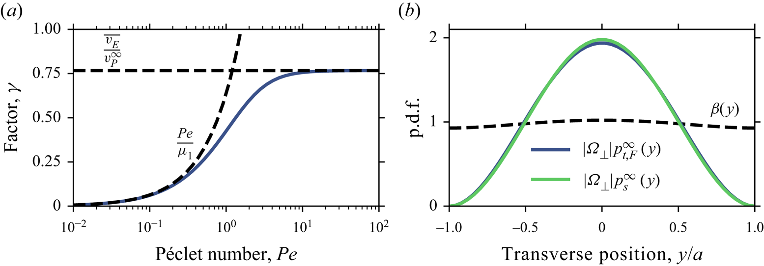
Equilibrium surviving mass and breakthrough p.d.f.s $p_t^\infty$ and $p_s^\infty$ in the 2-D channel, for (a) $\textit {Da}=10^{-1}$, (b) $\textit {Da}=1$, and (c) $\textit {Da}=10$. Symbols show the results of numerical simulations. The theoretical predictions approximate the breakthrough p.d.f. $p_s^\infty$ as the flux-weighted p.d.f. $p_{t,F}^\infty$ as discussed in the text. The solid lines in (a,c) show the analytical limit forms (E3) and (E5) for low $\textit {Da}$, and (E4) and (E6) for high $\textit {Da}$, respectively. The solid lines in (b) show the analytical solutions (4.3) and (4.5) with $\mu _1$ computed numerically according to (4.1d).

4.1.2. Velocity

Using (2.2), (3.8) and (4.3), we determine the asymptotic mean of the fixed-time velocity p.d.f. as

(4.13)\begin{equation} \frac{v_t^\infty}{\overline{v_E}} = 3\,\frac{1-\mu_1\cot\mu_1}{\mu_1^2} =\frac{3}{2}\,\frac{2\,\textit{Da}-\mu_1^2}{\textit{Da}\,\mu_1^2}. \end{equation}

As discussed in § 3.2, this is smaller than the mean plume velocity $v_P^\infty$, which describes the rate of change of the plume centre of mass at late times. We find from (3.17) and (4.8) that

(4.14)\begin{equation} \frac{v_P^\infty}{\overline{v_E}} = \frac{16\,\textit{Da}^2}{\mu_1^4b_1}\int_{{-}1}^{1} {\rm d}u\,u^2\,(p_t^\infty)^2(u) = 1+\frac{3}{4\mu_1^2}-\frac{3+4\,\textit{Da}}{2\mu_1^2+4\,\textit{Da}\,(1+2\,\textit{Da})}. \end{equation}

This result is equivalent to that reported in Lungu & Moffatt (Reference Lungu and Moffatt1982). Using (4.3) for $p_t^\infty$, (4.11) for $\alpha _\infty \,\Delta m(y)/\overline {v_E}$, (4.13) and (4.14) for $v_t^\infty /\overline {v_E}$ and $v_P^\infty /\overline {v_E}$, and $\Delta m_W=\Delta m(\pm a)$, we find by direct calculation that (3.22) is satisfied as expected.

In line with the discussion for the breakthrough p.d.f., we approximate the true average breakthrough velocity $v_s^\infty$ by the flux-weighted mean $v_{t,F}^\infty$. Proceeding similarly to the calculation of $v_t^\infty$, using (3.11), we obtain

(4.15)\begin{equation} \frac{v_{t,F}^\infty}{\overline{v_F}} = \frac{15}{\mu_1^2}\left(1-\frac{\overline{v_E}}{v_t^\infty}\right). \end{equation}

These results are shown as a function of $\textit {Da}$ in figure 4(a) (see § E.2 for the derivation of the high- and low-$\textit {Da}$ forms). The 3-D case, discussed in detail in § 4.2, is shown in figure 4(b) for comparison.

Figure 4.

Equilibrium mean of the transverse velocity p.d.f. in time $v_t^\infty$, its flux-weighted counterpart $v_{t,F}^\infty$, mean plume velocity $v_P^\infty$, and mean breakthrough velocity $v_s^\infty$, as a function of $\textit {Da}$ for (a) the 2-D channel and (b) the 3-D channel. The solid lines corresponding to $v_t^\infty$, $v_P^\infty$ and $v_{t,F}^\infty$ are the analytical solutions (a) (4.13), (4.14) and (4.15), and (b) (4.24), (4.25) and (4.26). The corresponding dashed lines show the analytical limit forms for low and high $\textit {Da}$: (a) (E7), (E9) and (E11), and (E8), (E10) and (E12); (b) (F7), (F9) and (F11), and (F8), (F10) and (F12). Solid lines corresponding to $v_s^\infty$ employ (3.28), together with (4.10) for (a) and (4.23) for (b); these lines use Péclet number $\textit {Pe}\to \infty$. Symbols show the results of numerical simulations for $\textit {Da}=10^{-1}$, $1$ and $10$.

It is interesting to note that for both the 2-D and 3-D channels, we have $\overline {v_E}<\overline {v_F}< v_t^\infty < v_{t,F}^\infty < v_s^\infty < v_P^\infty$ as $\textit {Da}\to \infty$. In this high-$\textit {Da}$ limit, there is a noticeable difference corresponding to an increase of approximately $7\,\%$ and $13\,\%$ between $v_t^\infty$ and $v_P^\infty$ in two and three dimensions, respectively. The plume velocity $v_P^\infty$ differs from the fixed-time flux-weighted velocity $v_{t,F}^\infty$ by only approximately $1\,\%$ and $2\,\%$, respectively, and the fixed-time average velocity $v_t^\infty$ is similar to the Eulerian flux-weighted mean velocity $\overline {v_F}$ rather than to the Eulerian mean velocity $\overline {v_E}$, differing by about $1\,\%$ in the 2-D case, and $4\,\%$ in the 3-D case. The average breakthrough velocity $v_s^\infty$ is approximately halfway between $v_P^\infty$ and $v_{t,F}^\infty$ in both cases. This should be contrasted with the conservative problem, for which $v_t^\infty =v_P^\infty =\overline {v_E}$ and $v_s^\infty =v_{t,F}^\infty =\overline {v_F}$. As shown in table 2, $\overline {v_F}$ is larger than the mean flow velocity $\overline {v_E}$ by $20\,\%$ and approximately $33\,\%$ in two and three dimensions; thus the mean plume velocity increases by approximately $30\,\%$ and $56\,\%$ as $\textit{Da} \to \infty$.

Table 2.

Eulerian and flux-weighted Eulerian flow velocity p.d.f.s and associated quantities for Poiseuille flow between two flat plates (spatial dimension $d=2$) and in a cylindrical channel ($d=3$).

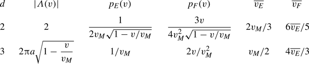
It is easy to see that the relationship $\overline {v_E}\leq \overline {v_F}$ always holds, with the equality holding if and only if the flow is uniform, due to fact that $\overline {v_F}$ assigns more weight to higher velocities. The same argument shows that $v_t^\infty \leq v _{t,F}^\infty$, and similarly, because breakthrough at fixed distance is naturally associated with a flux-weighting according to the local velocities, $v_t^\infty \leq v _s^\infty$. Since reaction happens at the channel walls, it leads to an increase of the velocities sampled by the plume, and therefore to an increase in the different Lagrangian (i.e. associated with sampling by the solute rather than characteristic of the flow) average velocities $v_t^\infty$, $v_{t,F}^\infty$, $v_s^\infty$ and $v_P^\infty$. Thus it is also easy to see that for the reactive problem, $\overline {v_E}< v_t^\infty,v_P^\infty$ and $\overline {v_F}< v_{t,F}^\infty,v_s^\infty$. We have seen that the inequality $v_{t,F}^\infty < v_s^\infty$ of two averages that are identical for the conservative problem arises from the interaction between the subleading moment discrepancy $\Delta m$ and reaction. Indeed, breakthrough is favoured where $\Delta m>0$, because the earlier arrival of Lagrangian trajectories at these positions means a shorter exposure to reaction; see (3.26). Given that $\Delta m\neq 0$, it is intuitive that the mean plume position for a given transverse position is larger where the flow velocity is larger. This mechanism acts in addition to the natural flux-weighting associated with breakthrough, and leads to $v_{t,F}^\infty < v_s^\infty$. For a similar reason, $v_t^\infty < v_P^\infty$; see (3.15). It should be noted that these qualitative arguments are not sufficient to ensure that for sufficiently fast reaction, the fixed-time averages $v_P^\infty$ and $v_t^\infty$ become larger than the flux-weighted Eulerian average $\overline {v_F}$, and similarly that $v_P^\infty$ becomes larger than both the Lagrangian flux-weighted average $v_{t,F}^\infty$ and the breakthrough average $v_s^\infty$, as we observe in figure 4. In other words, this discussion does not guarantee that this happens at finite $\textit {Da}$ for an arbitrary flow configuration.

We also note in this context that the inequality of Lagrangian and Eulerian average velocities is not limited to the reactive problem when considering early times. For the conservative problem, the classical Taylor dispersion picture implies that the asymptotic fixed-time transverse average velocity and the plume velocity both equal the average flow velocity $\overline {v_E}$, and similarly the average flux-weighted and breakthrough velocities equal $\overline {v_F}$. However, this is not true at pre-asymptotic times, when these quantities may differ as the initial plume deforms as it samples the flow, and complex pre-asymptotic distributions of transverse concentration and breakthrough may develop (Guan & Chen Reference Guan and Chen2024).

Next, we turn to the asymptotic velocity p.d.f.s. For the fixed-time p.d.f., using (3.6), (3.7) and (4.3), we obtain

(4.16)\begin{align} \frac{p_{v_t}^\infty(v)}{p_E(v)} = \frac{\mu_1^2}{2\,\textit{Da}}\left(\cos\left[\mu_1\left(1+\sqrt{1-\frac{v}{v_M}}\right)\right]+\frac{2\,\textit{Da}}{\mu_1}\sin\left[\mu_1\left(1+\sqrt{1-\frac{v}{v_M}}\right)\right]\right). \end{align}

Recall that the maximum velocity is $v_M=3\overline {v_E}/2$ for two dimensions. For $v\ll v_M$, we find by Taylor expansion that the low-velocity behaviour is flat, as for the conservative case. However, as $\textit {Da}\to \infty$ and $\mu _1\to {\rm \pi}/2$, the $v$-independent term vanishes. The low-velocity plateau, which accounts for contributions from the shear layer near the channel walls, is thus lower for higher $\textit {Da}$, and occurs for smaller $v$. The approach to this plateau is $\sim v$, and the scaling of the p.d.f. thus becomes linear in $v$ as $\textit {Da}\to \infty$. For $v\approx v_M$, corresponding to positions near the centre of the channel, we have $p_{v_t}^\infty (v)\sim 1/\sqrt {v-v_M}$ as for the conservative case, irrespective of $\textit {Da}$ (see § E.2 for further details on the low- and high-$\textit {Da}$ limits).

In line with the results for the breakthrough p.d.f., we approximate the true velocity p.d.f. $p_{v_s}^\infty$ associated with breakthrough at fixed distance by the flux-weighted p.d.f. $p_{v_t,F}^\infty$. Flux-weighting (4.16) and using (4.13), we find

(4.17)\begin{align} \frac{p_{v_t,F}^\infty(v)}{p_F(v)}=\frac{\mu_1^4}{6\,\textit{Da}-3\mu_1^2}\left(\cos\left[\mu_1\left(1\!+\!\sqrt{1-\frac{v}{v_M}}\right)\right] \!+\!\frac{2\,\textit{Da}}{\mu_1}\sin\left[\mu_1\left(1\!+\!\sqrt{1\!-\frac{v}{v_M}}\right)\right]\right). \end{align}

The low-velocity scaling is now linear for finite $\textit {Da}$, and becomes quadratic as $\textit {Da}\to \infty$. As before, for high velocities $v\approx v_M$, the scaling is $p_{v_t,F}^\infty (v)\sim 1/\sqrt {v-v_M}$, irrespective of $\textit {Da}$. The flux-weighted approximation agrees well with numerical simulations, as can be seen in figure 5.

Figure 5.

Equilibrium velocity p.d.f. in time $p_{v_t}^\infty$ and breakthrough velocity p.d.f. $p_{v_s}^\infty$ in the 2-D channel, for (a) $\textit {Da}=10^{-1}$, (b) $\textit {Da}=1$, and (c) $\textit {Da}=10$. Symbols show the results of numerical simulations. The theoretical predictions approximate $p_{v_s}^\infty$ as the flux-weighted p.d.f. $p_{v_t,F}^\infty$ as discussed in the text. The solid lines in (a,c) show the analytical limit forms (E13) and (E15) for low $\textit {Da}$, and (E14) and (E16) for high $\textit {Da}$, respectively. The solid lines in (b) show the analytical solutions (4.16) and (4.17), with $\mu _1$ computed numerically according to (4.1d). Dotted lines show the Eulerian and flux-weighted Eulerian velocity p.d.f.s $p_E(v)$ and $p_F(v)$, which equal $p_{v_t}^\infty$ and $p_{v_s}^\infty =p_{v_t,F}^\infty$ for the conservative problem.

4.2. Three-dimensional channel

Similarly to the 2-D case, decay modes of order higher than the first can be neglected at late times for transport in a cylindrical channel. Furthermore, in this case, symmetry ensures that any angular variability in the initial concentration along the channel cross-section vanishes at late times. The late-time solution for transverse concentrations is thus associated with the slowest radial decay mode and is given by (Polyanin & Nazaikinskii Reference Polyanin and Nazaikinskii2016)

(4.18a) \begin{align} c_\perp(\boldsymbol{x}_\perp, t) &= \frac{2}{a^2\,{\rm J}_1^2(\mu_1)}\,\frac{(2\,\textit{Da})^2}{\mu_1^2+(2\,\textit{Da})^2}\exp\left(\frac{-\mu_1^2t}{2\tau_D}\right){\rm J}_0\left(\mu_1\,\frac{|\boldsymbol{x}_\perp|}{a}\right)\nonumber\\ &\quad \times \int_0^a {\rm d}r\, r\, {\rm J}_0\left(\mu_1\,\frac{r}{a}\right)c_\perp(r, 0), \end{align}

where ${\rm J}_\nu$ is the Bessel function of the first kind of order $\nu$, and $\mu _1$ is the smallest positive root of

(4.18b)\begin{equation} \mu\,{\rm J}_1(\mu) = 2\,\textit{Da}\,{\rm J}_0(\mu). \end{equation}

Using the well-known recurrence relation $2\alpha \,{\rm J}_\alpha (x)/x = {\rm J}_{\alpha -1}(x)+{\rm J}_{\alpha +1}(x)$ (Abramowitz & Stegun Reference Abramowitz and Stegun1964) for $\alpha =1, 2$, we find that the latter is equivalent to

(4.18c,d)\begin{equation} {\rm J}_2(\mu) = \frac{4\,\textit{Da}-\mu^2}{\mu^2}\,{\rm J}_0(\mu), \quad{\rm J}_3(\mu) = 2\,\frac{8\,\textit{Da}-2\mu^2-\textit{Da}\,\mu^2}{\mu^3}\,{\rm J}_0(\mu). \end{equation}

The behaviour of $\mu _1$ as a function of $\textit {Da}$ is shown in figure 1(b); see § F.1 for the derivation of the asymptotic forms. Note that the $n$th radial mode decays exponentially at rate $\mu _n^2/(2\tau _D)$ as for the 2-D case, although the values of $\mu _n$ are different because they now solve (4.18b).

4.2.1. Surviving mass and breakthrough

From (4.18a), we obtain the surviving mass p.d.f.

(4.19)\begin{equation} p_t^\infty(\boldsymbol{x}_\perp) = \frac{\mu_1}{2{\rm \pi} a^2}\,\frac{{\rm J}_0(\mu_1|\boldsymbol{x}_\perp|/a)}{{\rm J}_1(\mu_1)} . \end{equation}

Again, we conclude in particular that an equilibrium form independent of the initial condition exists for all $\textit {Da}$, including $\textit {Da}\to \infty$. As before, the asymptotic reaction rate is given by

(4.20)\begin{equation} \alpha^\infty = \frac{\mu_1^2}{2\tau_D}. \end{equation}

Flux-weighting, we find

(4.21)\begin{equation} p_{t,F}^\infty(\boldsymbol{x}_\perp) = \frac{\textit{Da}\,\mu_1^2}{4\,\textit{Da}-\mu_1^2}\left(1-\frac{|\boldsymbol{x}_\perp|^2}{a^2}\right)p_t^\infty(\boldsymbol{x}_\perp); \end{equation}

see also the result for the fixed-time average velocity in (4.24) below. The limiting forms of these two p.d.f.s for $\textit {Da}\to 0$ and $\textit {Da}\to \infty$ are discussed in § F.1.

To find the breakthrough p.d.f. $p_s^\infty$, we must solve (3.20). As for the 2-D case, we assume that the initial condition $f(\boldsymbol {x}_\perp,0)\propto \int {{\rm d}\kern0.06em x}\,x\,c(x,\boldsymbol {x}_\perp,0)$ does not depend on $\boldsymbol {x}_\perp$, and we set $f(\boldsymbol {x}_\perp, 0)=0$ without further loss of generality. Analogously to the 2-D channel, the solution for $t\gg 2\tau _D/(\mu _2^2-\mu _1^2)$ is now (Polyanin & Nazaikinskii Reference Polyanin and Nazaikinskii2016)

(4.22)\begin{align} f(\boldsymbol{x}_\perp,t) &=\frac{8{\rm \pi}^2a^2 \mu_1^{{-}2} t\, p_t^\infty(\boldsymbol{x}_\perp)}{1+(\mu_1/2\,\textit{Da})^2} \int_{0}^{a} {\rm d}r\,r(p_t^\infty)^2(r)\,v_E(r) \nonumber\\ &\quad +\frac{2}{a^2\alpha^\infty}\sum_{n\geq 2}\frac{{\rm J}_1^{{-}2}(\mu_n)\,{\rm J}_0(\mu_n\,|\boldsymbol{x}_\perp|/a)}{1+(\mu_n/2\,\textit{Da})^2}\,\frac{\mu_1^2}{\mu_n^2-\mu_1^2}\int_{0}^{a} {\rm d}r\,r\,p_t^\infty(r)\,{\rm J}_0(\mu_n r/a)\,v_E(r). \end{align}

As before, the first term is associated with the mean plume velocity (see below), and from (3.19a,b) and (3.21) we conclude from the second term that

(4.23)\begin{align} \frac{\alpha^\infty}{\overline{v_E}}\,\Delta m(\boldsymbol{x}_\perp) &={-}4\sum_{n\geq 2}\frac{{\rm J}_0(\mu_n\,|\boldsymbol{x}_\perp|/a)}{{\rm J}_1^2(\mu_n)\,{\rm J}_0(\mu_1\,|\boldsymbol{x}_\perp|/a)}\, \frac{(2\,\textit{Da})^2}{(2\,\textit{Da})^2+\mu_n^2}\,\frac{\mu_1^2}{\mu_n^2-\mu_1^2}\nonumber\\ &\quad\times\int_{0}^{1} {\rm d}u\,u^3\,{\rm J}_0(\mu_1 u)\,{\rm J}_0(\mu_n u). \end{align}

We are not aware of a closed-form solution for either the integral or the sum in this case.

Recall that the mean-position discrepancy affects the breakthrough p.d.f. $p_s^\infty$ through the factor $\beta (\boldsymbol {x}_\perp )$ in (3.26). The $\beta$ profiles for different values of the Péclet number at infinite $\textit {Da}$ are shown in figure 6(a), along with a comparison between the resulting $p_s^\infty$ and the flux-weighted p.d.f. $p_{t,F}^\infty$ in figure 6(b). Although the difference to the flux-weighted p.d.f. is not dramatic, it is substantially more pronounced than in the 2-D case, and clearly discernible at the channel centre. At $\textit {Pe}=2$, the results are similar to those for $\textit {Pe}\to \infty$, which explains the good agreement found between simulations at $\textit {Pe}=2$ and theory for $\textit {Pe}\to \infty$ for the mean breakthrough velocity in figure 4(b). The results for the surviving mass and breakthrough p.d.f.s are shown in figure 7 for different $\textit {Da}$ at $\textit {Pe}=2$. As expected, the differences between $p_s^\infty$ and $p_{t,F}^\infty$ become more pronounced with increasing $\textit {Da}$, but are already visible at $\textit {Da}=10^{-1}$.

Figure 6.

Effect of the mean-position discrepancy $\Delta m(\boldsymbol {x}_\perp )$ on the breakthrough p.d.f. $p_s^\infty$ for the 3-D channel. The mean-position discrepancy generates differences between the flux-weighted p.d.f. $p_{t,F}^\infty$ and the true breakthrough p.d.f. $p_s^\infty$ through the factor $\beta (\boldsymbol {x}_\perp )$ in (3.26). (a) Behaviour of $\beta$ in the limit of infinite $\textit {Da}$, for different values of Péclet number $\textit {Pe}$. (b) Comparison of the resulting $p_s^\infty$ ((3.26) and (4.23), using terms up to $n=6$ in the sum according to the values of $\mu _n$ reported in Carslaw & Jaeger Reference Carslaw and Jaeger1986) to $p_{t,F}^\infty$ (F6).

Figure 7.

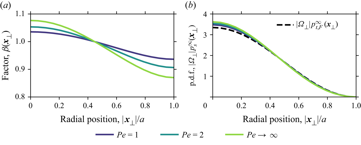
Equilibrium surviving mass and breakthrough p.d.f.s $p_t^\infty$ and $p_s^\infty$, and flux-weighted mass p.d.f. $p_{t,F}^\infty$, in the 3-D channel, for (a) $\textit {Da}=10^{-1}$, (b) $\textit {Da}=1$, and (c) $\textit {Da}=10$. Symbols show the results of numerical simulations. The solid lines in (a,c) for $p_t^\infty$ and $p_{t,F}^\infty$ show the analytical limiting forms (F3) and (F5) for low $\textit {Da}$, and (F4) and (F6) for high $\textit {Da}$. The corresponding solid lines in (b) show the analytical solutions (4.19) and (4.21), with $\mu _1$ computed numerically according to (4.18b). In all plots, the solid lines representing $p_s^\infty$ are computed using (3.26) and (4.23), using terms up to $n=6$ in the sum according to the values of $\mu _n$ reported in Carslaw & Jaeger (Reference Carslaw and Jaeger1986).

4.2.2. Velocity

Proceeding as for the 2-D case, but integrating (3.8) in polar coordinates and consulting table 2 for the 3-D case, we obtain for the asymptotic mean of the fixed-time velocity p.d.f.:

(4.24)\begin{equation} \frac{v_t^\infty}{\overline{v_E}} = 2\,\frac{4\,\textit{Da}-\mu_1^2}{\textit{Da}\,\mu_1^2}. \end{equation}

Using (4.22), arguments similar to those for the 2-D case lead to the asymptotic plume velocity

(4.25)\begin{align} \frac{v_P^\infty}{\overline{v_E}} = \frac{8{\rm \pi}^2}{\mu_1^2}\,\frac{(2\,\textit{Da})^2}{\mu_1^2+(2\,\textit{Da})^2}\int_0^a {\rm d}r\, r (p_t^\infty)^2(r)\,v_E(r) = \frac{4}{3}\left(1+\frac{1}{\mu_1^2}-\frac{1+2\,\textit{Da}}{\mu_1^2+(2\,\textit{Da})^2}\right), \end{align}

This result is equivalent to that reported in Lungu & Moffatt (Reference Lungu and Moffatt1982). For the flux-weighted mean velocity, we find

(4.26)\begin{equation} \frac{v_{t,F}^\infty}{\overline{v_F}} = \frac{24}{\mu_1^2}\left(1-\frac{\overline{v_E}}{v_t^\infty}\right). \end{equation}

The different mean velocities are shown as a function of $\textit {Da}$ in figure 4(b); see also the associated discussion in §§ 4.1.2 and F.2 for the limiting forms at low and high $\textit {Da}$.

We now turn to the asymptotic velocity p.d.f.s, again proceeding as for the one-dimensional case. First, according to (3.6), the fixed-time p.d.f. is given by

(4.27)\begin{equation} \frac{p_{v_t}^\infty(v)}{p_E(v)} = \frac{\mu_1}{2{\rm \pi} a^2\,{\rm J}_1(\mu_1)}\,{\rm J}_0\left(\mu_1\sqrt{1-\frac{v}{v_M}}\right). \end{equation}

Note that in this case, the Eulerian p.d.f. $p_E(v)=1/v_M$ is independent of $v$; see table 2. Finally, for the flux-weighted p.d.f., we have

(4.28)\begin{equation} \frac{p_{v_t,F}^\infty(v)}{p_F(v)} = \frac{\mu_1^3}{4{\rm \pi} a^2\,{\rm J}_1(\mu_1)}\,\frac{\textit{Da}}{4\,\textit{Da}-\mu_1^2}\,{\rm J}_0\left(\mu_1\sqrt{1-\frac{v}{v_M}}\right). \end{equation}

These velocity p.d.f.s are illustrated in figure 8 (see § F.2 for low- and high-$\textit {Da}$ forms) along with the breakthrough velocity p.d.f. $p_{v_s}^\infty$ from (3.27) that takes into account the mean-position discrepancy (4.23). The differences between $p_{v_s}^\infty$ and $p_{v_t,F}^\infty$ are in line with the discussion of the breakthrough p.d.f. $p_s^\infty$; see figure 7.

Figure 8.

Equilibrium velocity p.d.f. at fixed time $p_{v_t}^\infty$, corresponding flux-weighted p.d.f. $p_{v_t,F}^\infty$, and breakthrough velocity p.d.f. $p_{v_s}^\infty$ in the 3-D channel, for (a) $\textit {Da}=10^{-1}$, (b) $\textit {Da}=1$, and (c) $\textit {Da}=10$. Symbols show the results of numerical simulations. The solid lines associated with $p_{v_t}^\infty$ and $p_{v_t,F}^\infty$ in (a,c) show the analytical limit forms (F13) and (F15) for low $\textit {Da}$, and (F14) and (F16) for high $\textit {Da}$. The corresponding solid lines in (b) show the analytical solutions (4.27) and (4.28), with $\mu _1$ computed numerically according to (4.18b). The solid lines associated with $p_{v_s}^\infty$ use (3.27) in all plots, with $p_s$ computed as in figure 7. Dotted lines show the Eulerian and flux-weighted Eulerian p.d.f.s, which equal $p_{v_t}^\infty$ and $p_{v_s}^\infty =p_{v_t,F}^\infty$ for the conservative problem.