


1. Introduction
For micron-sized particles, the presence of fluid flow can enhance mass transport due to the interplay between advection and diffusion. A classical example of this coupling effect is Taylor dispersion, where Brownian solutes in pressure-driven flows exhibit enhanced longitudinal dispersion compared with the molecular diffusivity (Taylor Reference Taylor1953, Reference Taylor1954a , Reference Taylorb ; Aris Reference Aris1956). Since the work of Taylor (Reference Taylor1953), a generalised Taylor dispersion (GTD) framework has been developed to study a variety of transport phenomena. These include complex geometries, spatial and temporal periodicity and active (i.e. self-propelled) particle dynamics (Brenner Reference Brenner1980; Shapiro & Brenner Reference Shapiro and Brenner1990; Hill & Bees Reference Hill and Bees2002; Zia & Brady Reference Zia and Brady2010; Brenner Reference Brenner2013; Alonso-Matilla, Chakrabarti & Saintillan Reference Alonso-Matilla, Chakrabarti and Saintillan2019; Peng & Brady Reference Peng and Brady2020; Peng Reference Peng2024).
Active particles differ from passive solutes in that each unit is capable of self-propulsion (Schweitzer, Ebeling & Tilch Reference Schweitzer, Ebeling and Tilch1998; Romanczuk et al. Reference Romanczuk, Bär, Ebeling, Lindner and Schimansky-Geier2012). The interplay between self-propulsion and fluid flow gives rise to a rich and often non-intuitive dynamics that is absent in passive Brownian systems (Romanczuk et al. Reference Romanczuk, Bär, Ebeling, Lindner and Schimansky-Geier2012; Bechinger et al. Reference Bechinger, Di Leonardo, Löwen, Reichhardt, Volpe and Volpe2016; Gomez-Solano, Blokhuis & Bechinger Reference Gomez-Solano, Blokhuis and Bechinger2016; Chandragiri et al. Reference Chandragiri, Doostmohammadi, Yeomans and Thampi2020; Jing et al. Reference Jing, Zöttl, Clément and Lindner2020; Plan et al. Reference Plan, Yeomans and Doostmohammadi2020; Chakraborty et al. Reference Chakraborty, Maiti, Sharma and Dey2022; Choudhary et al. Reference Choudhary, Paul, Rühle and Stark2022). One example where this dynamics plays a crucial role is the transport behaviour of microswimmers, which is important for understanding both natural and engineered systems, such as infection by motile bacteria (Siitonen & Nurminen Reference Siitonen and Nurminen1992; Lane et al. Reference Lane, Lockatell, Monterosso, Lamphier, Weinert, Hebel, Johnson and Mobley2005), formation of biofilms (Rusconi et al. Reference Rusconi, Lecuyer, Guglielmini and Stone2010; Kim et al. Reference Kim, Drescher, Pak, Bassler and Stone2014), drug delivery (Park et al. Reference Park, Zhuang, Yasa and Sitti2017; Díez et al. Reference Díez, Lucena-Sánchez, Escudero, Llopis-Lorente, Villalonga and Martinez-Manez2021; Lin et al. Reference Lin, Yu, Chen and Gao2021; Sridhar et al. Reference Sridhar, Podjaski, Alapan, Kröger, Grunenberg, Kishore, Lotsch and Sitti2022), therapeutic treatments (Ghosh et al. Reference Ghosh, Xu, Gupta and Gracias2020) and environmental remediation (Soler et al. Reference Soler, Magdanz, Fomin, Sanchez and Schmidt2013; Urso, Ussia & Pumera Reference Urso, Ussia and Pumera2023).
Transport of active particles often occurs in confined geometries, where Poiseuille flow is a common flow profile, and considerable work has focused on how active matter behaves in such environments (Zöttl & Stark Reference Zöttl and Stark2012, Reference Zöttl and Stark2013; Apaza & Sandoval Reference Apaza and Sandoval2016; Junot et al. Reference Junot, Figueroa-Morales, Darnige, Lindner, Soto, Auradou and Clément2019; Mathijssen et al. Reference Mathijssen, Figueroa-Morales, Junot, Clément, Lindner and Zöttl2019; Anand & Singh Reference Anand and Singh2021; Chuphal, Sahoo & Thakur Reference Chuphal, Sahoo and Thakur2021; Choudhary et al. Reference Choudhary, Paul, Rühle and Stark2022; Khatri & Burada Reference Khatri and Burada2022; Walker et al. Reference Walker, Ishimoto, Moreau, Gaffney and Dalwadi2022; Ganesh et al. Reference Ganesh, Douarche, Dentz and Auradou2023; Valani, Harding & Stokes Reference Valani, Harding and Stokes2024). For instance, in channels, active particles exhibit upstream swimming in Poiseuille flow (Kaya & Koser Reference Kaya and Koser2012; Kantsler et al. Reference Kantsler, Dunkel, Blayney and Goldstein2014; Ezhilan & Saintillan Reference Ezhilan and Saintillan2015; Omori & Ishikawa Reference Omori and Ishikawa2016). Owing to their upstream motility, Escherichia coli introduced downstream causes upstream contamination in initially clean microfluidic channels (Figueroa-Morales et al. Reference Figueroa-Morales, Rivera, Soto, Lindner, Altshuler and Clément2020). Further investigations by Mathijssen et al. (Reference Mathijssen, Figueroa-Morales, Junot, Clément, Lindner and Zöttl2019) on bacterial motion near channel surfaces revealed that E. coli engages in distinct rheotaxis regimes depending on the shear rate. With increasing shear, the bacteria transition from upstream swimming to oscillatory rheotaxis, and ultimately to a coexistence of rheotaxis aligned with both positive and negative vorticity directions.
While these studies were primarily focused on steady flows, biologically relevant systems are often governed by time-dependent flow conditions. McDonald (Reference McDonald1955) experimentally studied the relationship between pulsatile pressure and blood flow in arteries, analysing the phasic variations in arterial flow during each cardiac cycle. Inspired by the study of McDonald (Reference McDonald1955), Womersley (Reference Womersley1955) investigated the velocity, rate of flow and viscous drag in arteries by considering a time-periodic pressure gradient. The primary factors governing such flows include the pulsatile pressure generated by the heart, the structural and mechanical properties of the vascular walls and the flow behaviour of blood (Secomb Reference Secomb2016).
Early studies on longitudinal dispersion of passive contaminants in oscillatory pressure-driven flows were carried out by Chatwin (Reference Chatwin1975, Reference Chatwin1977). Later, Watson (Reference Watson1983) derived analytical solutions for the long-time effective dispersivity in oscillatory flows within both pipes and rectangular channels. His results showed that the effective dispersivity decreases monotonically with increasing flow frequency. Subsequently, Mazumder & Das (Reference Mazumder and Das1992) investigated how boundary absorption and heterogeneous reactions influence contaminant dispersion in both steady and oscillatory flows. The significance of such boundary interactions lies in their relevance to processes such as deposition and transport across semi-permeable membranes. More recently, Chu et al. (Reference Chu, Garoff, Przybycien, Tilton and Khair2019) developed a macro-transport theory for two-dimensional flows in a parallel plate channel with alternating shear-free and no-slip regions. They considered both steady and oscillatory flow components to study the transport coefficients of passive particles. Later, they extended their analysis to eccentric annuli (Chu et al. Reference Chu, Garoff, Tilton and Khair2020) where they showed that the maximum dispersion observed in a time-oscillatory flow can be achieved by applying a slowly oscillating flow in an annulus with large eccentricity. Hettiarachchi et al. (Reference Hettiarachchi, Hsu, Harris and Linninger2011) used experiments and simulations to show that pulsatile cerebrospinal fluid significantly enhances drug dispersion in the spinal cord relative to no flow.
Although the dispersion of passive particles in oscillatory flows has been widely studied, much less is known about the transport of microswimmers in oscillatory flows. Recently, using experiments and simulations, Caldag & Bees (Reference Caldag and Bees2025) showed that oscillatory flow can lead to a non-trivial dispersion dynamics in gyrotactic swimmers. Wang et al. (Reference Wang, Jiang, Zeng, Wu and Wang2025) studied Taylor–Aris dispersion of active particles in oscillatory channel flows and showed that spherical non-gyrotactic swimmers can exhibit either enhanced or reduced diffusivity relative to passive solutes due to disruption of cross-streamline migration associated with Jeffery orbits. Lagoin et al. (Reference Lagoin, Lacherez, de Tournemire, Badr, Amarouchene, Allard and Salez2025) experimentally investigated the motility and dispersion of Chlamydomonas reinhardtii microalgae within a rectangular microfluidic channel under sinusoidal Poiseuille flow, showing that velocity fluctuations and the dispersion coefficient increase with flow amplitude, with weak dependencies on flow periodicity. In this paper, we consider the dispersion of active Brownian particles (ABPs) in time-periodic pressure-driven Poiseuille flow through planar channels. We apply the GTD theory of Peng & Brady (Reference Peng and Brady2020), originally developed for ABPs in steady flow, to characterise the long-time longitudinal dispersion of ABPs in oscillatory flow. Due to the time-periodic nature of the flow, an additional time average over one oscillation period is performed to define the time-averaged dispersion coefficient (Chatwin Reference Chatwin1975, Reference Chatwin1977; Watson Reference Watson1983). In the weak-swimming limit, characterised by a small swim Péclet number ( $\textit{Pe}_s \ll 1$
), we show that the first effect of swimming on longitudinal dispersion appears at
$\textit{Pe}_s \ll 1$
), we show that the first effect of swimming on longitudinal dispersion appears at $O(\textit{Pe}_s^2)$
. Depending on the flow Péclet number (
$O(\textit{Pe}_s^2)$
. Depending on the flow Péclet number ( $\textit{Pe}$
) and oscillation frequency, the
$\textit{Pe}$
) and oscillation frequency, the $O(\textit{Pe}_s^2)$
contribution can be either positive or negative. As such, activity can either enhance or hinder longitudinal dispersion in oscillatory Poiseuille flow compared with passive Brownian particles. For arbitrary swim speeds, numerical solutions of the governing equations are used to characterise the dispersion as a function of the flow speed, swim speed and oscillation frequency. Numerical results are validated against Brownian dynamics (BD) simulations.
$O(\textit{Pe}_s^2)$
contribution can be either positive or negative. As such, activity can either enhance or hinder longitudinal dispersion in oscillatory Poiseuille flow compared with passive Brownian particles. For arbitrary swim speeds, numerical solutions of the governing equations are used to characterise the dispersion as a function of the flow speed, swim speed and oscillation frequency. Numerical results are validated against Brownian dynamics (BD) simulations.
2. Problem formulation
2.1. The Smoluchowski equation
We consider the long-time transport behaviour of ABPs dispersed in a viscous Newtonian solvent confined between two parallel plates with a separation distance of $2H$
. In the dilute limit, we only consider the dynamics of a single ABP. The ABP is assumed to be spherical, and its radius is much smaller than the width of the channel. This allows us to treat the ABP as a ‘point’ particle. An ABP self-propels with a constant swim speed
$2H$
. In the dilute limit, we only consider the dynamics of a single ABP. The ABP is assumed to be spherical, and its radius is much smaller than the width of the channel. This allows us to treat the ABP as a ‘point’ particle. An ABP self-propels with a constant swim speed $U_s$
in a body-fixed swimming direction
$U_s$
in a body-fixed swimming direction $\boldsymbol{q}$
(
$\boldsymbol{q}$
( $\boldsymbol{q}\boldsymbol{\cdot }\boldsymbol{q}=1$
). Due to rotational Brownian motion, the orientation vector
$\boldsymbol{q}\boldsymbol{\cdot }\boldsymbol{q}=1$
). Due to rotational Brownian motion, the orientation vector $\boldsymbol{q}$
undergoes stochastic reorientation. The configuration of an ABP at time
$\boldsymbol{q}$
undergoes stochastic reorientation. The configuration of an ABP at time $t$
is described by its position vector
$t$
is described by its position vector $\boldsymbol{x}$
and by the orientation vector
$\boldsymbol{x}$
and by the orientation vector $\boldsymbol{q}$
. We define
$\boldsymbol{q}$
. We define $P({\boldsymbol{x}}, \boldsymbol{q}, t)$
as the probability density function of finding the ABP at position
$P({\boldsymbol{x}}, \boldsymbol{q}, t)$
as the probability density function of finding the ABP at position $\boldsymbol{x}$
with orientation
$\boldsymbol{x}$
with orientation $\boldsymbol{q}$
at time
$\boldsymbol{q}$
at time $t$
. It satisfies the Smoluchowski equation
$t$
. It satisfies the Smoluchowski equation
 \begin{equation} \frac {\partial P}{\partial t} + \boldsymbol{\nabla }\boldsymbol{\cdot }\boldsymbol{j}_{\!T} + \boldsymbol{\nabla} _{\!R} \boldsymbol{\cdot }\boldsymbol{j}_{\!R}=0, \end{equation}
where $\boldsymbol{\nabla }= \partial /\partial {\boldsymbol{x}}$
and
$\boldsymbol{\nabla }= \partial /\partial {\boldsymbol{x}}$
and $\boldsymbol{\nabla} _{\!R} = \boldsymbol{q} \times \partial /\partial \boldsymbol{q}$
are the spatial and rotational gradient operators, respectively. In (2.1),
$\boldsymbol{\nabla} _{\!R} = \boldsymbol{q} \times \partial /\partial \boldsymbol{q}$
are the spatial and rotational gradient operators, respectively. In (2.1),
 \begin{equation} \boldsymbol{j}_{\!T} = U_s \boldsymbol{q} P + {\boldsymbol{u}}_{\!f} P - D_T \boldsymbol{\nabla }\!P, \end{equation}
 \begin{equation} \boldsymbol{j}_{\!R} = \boldsymbol{\varOmega }_{\!f} P -D_{\!R} \boldsymbol{\nabla} _{\!R} P, \end{equation}
where ${\boldsymbol{u}}_{\!f}$
is the background fluid velocity field,
${\boldsymbol{u}}_{\!f}$
is the background fluid velocity field, $D_T$
is the translational diffusivity of the ABP,
$D_T$
is the translational diffusivity of the ABP, $\boldsymbol{\varOmega }_{\!f} = ( {1}/{2})\boldsymbol{\nabla }\times {\boldsymbol{u}}_{\!f}$
is the flow-induced angular velocity and
$\boldsymbol{\varOmega }_{\!f} = ( {1}/{2})\boldsymbol{\nabla }\times {\boldsymbol{u}}_{\!f}$
is the flow-induced angular velocity and $D_{\!R}$
is the rotational diffusivity of the ABP. The inverse of
$D_{\!R}$
is the rotational diffusivity of the ABP. The inverse of $D_{\!R}$
,
$D_{\!R}$
, $\tau _{\!R} = 1/D_{\!R}$
, defines the reorientation time. At the channel walls, the no-flux boundary condition is satisfied (Ezhilan & Saintillan Reference Ezhilan and Saintillan2015; Peng & Brady Reference Peng and Brady2020)
$\tau _{\!R} = 1/D_{\!R}$
, defines the reorientation time. At the channel walls, the no-flux boundary condition is satisfied (Ezhilan & Saintillan Reference Ezhilan and Saintillan2015; Peng & Brady Reference Peng and Brady2020)
 \begin{equation} \boldsymbol{e}_y \boldsymbol{\cdot }\boldsymbol{j}_{\!T} =0, \quad y = \pm H, \end{equation}
where $\boldsymbol{e}_y$
is the unit normal to the channel walls. The longitudinal Cartesian coordinate is
$\boldsymbol{e}_y$
is the unit normal to the channel walls. The longitudinal Cartesian coordinate is $x$
and
$x$
and $y$
is the transverse coordinate.
$y$
is the transverse coordinate.
2.2. Oscillatory Poiseuille flow
For ease of reference, we provide a brief outline of the flow field derivation. We consider a one-dimensional flow, ${\boldsymbol{u}}_{\!f} = u(y,t){\boldsymbol{e}}_x$
, driven by a prescribed oscillatory pressure gradient along the channel (Womersley Reference Womersley1955). Here,
${\boldsymbol{u}}_{\!f} = u(y,t){\boldsymbol{e}}_x$
, driven by a prescribed oscillatory pressure gradient along the channel (Womersley Reference Womersley1955). Here, ${\boldsymbol{e}}_x$
is the unit basis vector in the longitudinal direction. The Navier–Stokes equations reduce to
${\boldsymbol{e}}_x$
is the unit basis vector in the longitudinal direction. The Navier–Stokes equations reduce to
 \begin{equation} \rho \frac {\partial u}{\partial t} = - \frac {\partial p}{\partial x} + \mu \frac {\partial ^2 u }{\partial y^2}, \end{equation}
where $\rho$
is the density of the fluid,
$\rho$
is the density of the fluid, $\mu$
is the dynamic viscosity of the fluid and the prescribed pressure gradient is given by
$\mu$
is the dynamic viscosity of the fluid and the prescribed pressure gradient is given by
 \begin{equation} - \frac {\partial p}{\partial x} = \frac {P_0}{H} \cos (\omega t). \end{equation}
In (2.6), $P_0$
is a reference pressure and
$P_0$
is a reference pressure and $\omega$
is the angular frequency of the actuation. One can show that the solution of (2.5) may be written as
$\omega$
is the angular frequency of the actuation. One can show that the solution of (2.5) may be written as $u(y,t) ={\operatorname {Re}} [ u^\prime (y) e^{i\omega t} ]$
, where
$u(y,t) ={\operatorname {Re}} [ u^\prime (y) e^{i\omega t} ]$
, where
 \begin{equation} u^\prime (y) = \frac {i P_0}{\rho H \omega } \left [-1 + \cosh \left ( (1+i)\lambda y \right ) {\textrm {sech}}\left ((1+i)\lambda H \right )\right ]\!. \end{equation}
In (2.7), $i=\sqrt {-1}$
is the imaginary unit,
$i=\sqrt {-1}$
is the imaginary unit, $\nu = \mu /\rho$
is the kinematic viscosity of the fluid and
$\nu = \mu /\rho$
is the kinematic viscosity of the fluid and $\lambda = \sqrt {\omega /(2\nu )}$
. The viscous length,
$\lambda = \sqrt {\omega /(2\nu )}$
. The viscous length, $1/\lambda = \sqrt {2\nu /\omega }$
, sets the scale over which the fluid momentum diffuses during one oscillation cycle of the applied pressure. The operator
$1/\lambda = \sqrt {2\nu /\omega }$
, sets the scale over which the fluid momentum diffuses during one oscillation cycle of the applied pressure. The operator $\operatorname {Re}$
extracts the real part of a complex quantity.
$\operatorname {Re}$
extracts the real part of a complex quantity.
In the zero-frequency limit, $\omega \to 0$
, we recover the steady Poiseuille flow as
$\omega \to 0$
, we recover the steady Poiseuille flow as
 \begin{equation} u(y,t) \to \frac {P_0H}{2 \mu } \left (1 - \frac {y^2}{H^2} \right )\!. \end{equation}
For convenience, we define the characteristic flow speed $U_{\!f} = P_0H/(2\mu )$
. Using this, we rewrite (2.7) as
$U_{\!f} = P_0H/(2\mu )$
. Using this, we rewrite (2.7) as
 \begin{equation} u^\prime (y) = \frac {i U_{\!f}}{(\lambda H)^2} \left [-1 + \cosh \left ( (1+i)\lambda y \right ) {\textrm {sech}}\left ((1+i)\lambda H \right )\right ]\!. \end{equation}
The angular velocity $\varOmega _{\!f}(y, t) = {\operatorname {Re}} [\varOmega ^\prime e^{i\omega t} ]$
, where
$\varOmega _{\!f}(y, t) = {\operatorname {Re}} [\varOmega ^\prime e^{i\omega t} ]$
, where
 \begin{equation} \varOmega ^\prime = - \frac {1}{2} \frac {\partial u^\prime }{\partial y} = \frac {(1-i) U_{\!f}}{2 \lambda H^2} \sinh \left ( (1+i)\lambda y \right ) {\textrm {sech}}\left ((1+i)\lambda H \right )\!. \end{equation}
2.3. Generalised Taylor dispersion theory
Taking the zeroth orientational moment of (2.1) gives the governing equation for the number density
 \begin{equation} \frac {\partial n}{\partial t} + \boldsymbol{\nabla }\boldsymbol{\cdot }\left ( {\boldsymbol{u}}_{\!f} n + U_s \boldsymbol{m} - D_T \boldsymbol{\nabla }n \right )=0, \end{equation}
where $n = \int _{\mathbb{S}} P {\text{d}\boldsymbol{q}}$
is the number density, and
$n = \int _{\mathbb{S}} P {\text{d}\boldsymbol{q}}$
is the number density, and $\boldsymbol{m} = \int _{\mathbb{S}} \boldsymbol{q} P {\text{d}\boldsymbol{q}}$
is the first moment, or polar order. Here,
$\boldsymbol{m} = \int _{\mathbb{S}} \boldsymbol{q} P {\text{d}\boldsymbol{q}}$
is the first moment, or polar order. Here, $\mathbb{S} = \{\boldsymbol{q} \, | \, \boldsymbol{q}\boldsymbol{\cdot }\boldsymbol{q} = 1\}$
denotes the unit sphere of orientations. In the following, we present a general derivation and then specialise to two dimensions. Since the channel is unbounded in the
$\mathbb{S} = \{\boldsymbol{q} \, | \, \boldsymbol{q}\boldsymbol{\cdot }\boldsymbol{q} = 1\}$
denotes the unit sphere of orientations. In the following, we present a general derivation and then specialise to two dimensions. Since the channel is unbounded in the $x$
direction, it is convenient to work in Fourier space. To derive a long-time effective transport equation, we first define the Fourier transform of a function
$x$
direction, it is convenient to work in Fourier space. To derive a long-time effective transport equation, we first define the Fourier transform of a function $f(x)$
as
$f(x)$
as $\hat {f}(k)=\int e^{-ikx} f(x) \text{d} x$
, where
$\hat {f}(k)=\int e^{-ikx} f(x) \text{d} x$
, where $k$
is the wavenumber. Following Peng & Brady (Reference Peng and Brady2020), one can show that
$k$
is the wavenumber. Following Peng & Brady (Reference Peng and Brady2020), one can show that
 \begin{equation} \frac {\partial \overline {n}}{\partial t} + k^2 D_T \overline {n} + ik \left (\overline {u(y,t)\hat {n}} +U_s \overline {\hat {m}_x} \right )=0, \end{equation}
where we have made use of the no-flux condition, and an overhead bar denotes the cross-sectional average
 \begin{equation} \overline {n}(k, t) = \frac {1}{2H}\int _{-H}^H \hat {n}(k,y,t) \text{d} y. \end{equation}
In (2.12), $\hat {m}_x = {\boldsymbol{e}}_x\boldsymbol{\cdot }\hat {\boldsymbol{m}}$
is the polar order in the
$\hat {m}_x = {\boldsymbol{e}}_x\boldsymbol{\cdot }\hat {\boldsymbol{m}}$
is the polar order in the $x$
direction in Fourier space.
$x$
direction in Fourier space.
Introducing the non-dimensional density or structure function $\hat {G}$
such that
$\hat {G}$
such that $\hat {P}(k, y, \boldsymbol{q}, t) = \overline {n}(k,t)\hat {G}(k,y,\boldsymbol{q},t)$
and the small-wavenumber expansion
$\hat {P}(k, y, \boldsymbol{q}, t) = \overline {n}(k,t)\hat {G}(k,y,\boldsymbol{q},t)$
and the small-wavenumber expansion $\hat {G} = g(y, \boldsymbol{q}, t) + ik\, b(y, \boldsymbol{q}, t) +O(k^2)$
, we obtain
$\hat {G} = g(y, \boldsymbol{q}, t) + ik\, b(y, \boldsymbol{q}, t) +O(k^2)$
, we obtain
 \begin{equation} \frac {\partial \overline {n}}{\partial t}+ ik U^{\textit{eff}}\overline {n} + k^2 D^{\textit{eff}}\overline {n} + O(k^3)=0, \end{equation}
where the effective drift and the effective longitudinal dispersivity are given by, respectively,
 \begin{equation} U^{\textit{eff}} = U^{\textit{eff}}(t) = U_s \overline {m_x^0} + \overline {un^0}, \end{equation}
 \begin{equation} D^{\textit{eff}} = D^{\textit{eff}}(t) = D_T - U_s\overline {\tilde {m}_x}-\overline {u\tilde {n}}. \end{equation}
In the small-wavenumber expansion, $g$
is the average field and
$g$
is the average field and $b$
is the displacement (or fluctuating) field. Note that
$b$
is the displacement (or fluctuating) field. Note that $b$
has units of length, e.g. displacement. We emphasise that terms of order
$b$
has units of length, e.g. displacement. We emphasise that terms of order $k^3$
and higher do not contribute to either the drift or the dispersion coefficient, as evidenced in (2.14). In general, a diffusive flux is proportional to the gradient of a concentration; equivalently, in a small-wavenumber expansion in Fourier space, it appears at second order in
$k^3$
and higher do not contribute to either the drift or the dispersion coefficient, as evidenced in (2.14). In general, a diffusive flux is proportional to the gradient of a concentration; equivalently, in a small-wavenumber expansion in Fourier space, it appears at second order in $k$
. Physically, a diffusivity describes only leading-order gradient transport and therefore cannot capture higher-order effects. Likewise, drift and diffusivity characterise only the lowest moments of the underlying probability distribution. To resolve the full probability distribution, one must retain higher-order moments. The orientational moments in (2.15) are given by
$k$
. Physically, a diffusivity describes only leading-order gradient transport and therefore cannot capture higher-order effects. Likewise, drift and diffusivity characterise only the lowest moments of the underlying probability distribution. To resolve the full probability distribution, one must retain higher-order moments. The orientational moments in (2.15) are given by
 \begin{equation} n^0 = \int _{\mathbb{S}} g {\text{d}\boldsymbol{q}}, \quad \mathrm{and}\quad \boldsymbol{m}^0=\int _{\mathbb{S}} \boldsymbol{q}\kern-1pt g{\text{d}\boldsymbol{q}}. \end{equation}
Similarly, in (2.16), we have
 \begin{equation} \tilde {n} = \int _{\mathbb{S}} b {\text{d}\boldsymbol{q}}, \quad \mathrm{and}\quad \tilde {\boldsymbol{m}}=\int _{\mathbb{S}} \boldsymbol{q} b{\text{d}\boldsymbol{q}}. \end{equation}
Different from the constant transport coefficients in Peng & Brady (Reference Peng and Brady2020), the long-time transport coefficients in (2.15) and (2.16) are time-dependent due to the oscillatory flow.
The governing equations and boundary conditions for $g$
and
$g$
and $b$
are derived in Peng & Brady (Reference Peng and Brady2020). For the average field, we have
$b$
are derived in Peng & Brady (Reference Peng and Brady2020). For the average field, we have
 \begin{equation} \frac {\partial g}{\partial t} + \frac {\partial }{\partial y}\left ( U_s q_y g -D_T \frac {\partial g}{\partial y}\right ) +\boldsymbol{\nabla} _{\!R}\boldsymbol{\cdot }\left ( \boldsymbol{\varOmega }_{\!f} g - D_{\!R} \boldsymbol{\nabla} _{\!R} g\right )=0, \end{equation}
and
 \begin{equation} U_s q_y g -D_T \frac {\partial g}{\partial y}=0, \quad y=\pm H. \end{equation}
The displacement field is governed by
 \begin{equation} \frac {\partial b}{\partial t} + \frac {\partial }{\partial y}\left ( U_s q_y b -D_T \frac {\partial b}{\partial y}\right ) +\boldsymbol{\nabla} _{\!R}\boldsymbol{\cdot }\left ( \boldsymbol{\varOmega }_{\!f} b - D_{\!R} \boldsymbol{\nabla} _{\!R} b\right )=\big(U^{\textit{eff}} - u-U_s q_x\big) g, \end{equation}
 \begin{equation} U_s q_y b -D_T \frac {\partial b}{\partial y}=0, \quad y=\pm H. \end{equation}
Noting that
 \begin{equation} \frac {1}{2H}\int _{-H}^H \text{d} y \int _{\mathbb{S}} \hat {G}{\text{d}\boldsymbol{q}}=1, \end{equation}
we have
 \begin{equation} \frac {1}{2H}\int _{-H}^H \text{d} y \int _{\mathbb{S}} g{\text{d}\boldsymbol{q}}=1, \quad \mathrm{and}\quad \frac {1}{2H}\int _{-H}^H \text{d} y \int _{\mathbb{S}} b {\text{d}\boldsymbol{q}}=0. \end{equation}
The above derivation of the GTD theory applies in both two and three dimensions. In the remainder of the paper, we restrict attention to two dimensions, where the orientation vector is parametrised as $\boldsymbol{q} = \cos \phi \,{\boldsymbol{e}}_x + \sin \phi \,{\boldsymbol{e}}_y$
, with
$\boldsymbol{q} = \cos \phi \,{\boldsymbol{e}}_x + \sin \phi \,{\boldsymbol{e}}_y$
, with $\phi \in [0, 2\pi )$
being the orientation angle. In two dimensions, the rotational gradient operator is given by
$\phi \in [0, 2\pi )$
being the orientation angle. In two dimensions, the rotational gradient operator is given by $\boldsymbol{\nabla} _{\!R} = {\boldsymbol{e}}_{z}( {\partial }/{\partial \phi })$
, where
$\boldsymbol{\nabla} _{\!R} = {\boldsymbol{e}}_{z}( {\partial }/{\partial \phi })$
, where ${\boldsymbol{e}}_z = {\boldsymbol{e}}_x \times {\boldsymbol{e}}_y$
.
${\boldsymbol{e}}_z = {\boldsymbol{e}}_x \times {\boldsymbol{e}}_y$
.
2.4. Non-dimensionalisation
We scale lengths with the channel half-width $H$
and time with the reorientation time
$H$
and time with the reorientation time $\tau _{\!R}$
. The system is governed by five non-dimensional parameters
$\tau _{\!R}$
. The system is governed by five non-dimensional parameters
 \begin{equation} \textit{Pe} = \frac {U_{\!f} \tau _{\!R}}{H}, \quad \textit{Pe}_s = \frac {U_s \tau _{\!R}}{H} = \frac {\ell }{H}, \quad \gamma = \frac {\sqrt {D_T\tau _{\!R}}}{H}=\frac {\delta }{H}, \end{equation}
 \begin{equation} \quad \chi = \omega \, \tau _{\!R}, \quad \kappa =\lambda H = \sqrt {\omega /(2\nu )}H, \end{equation}
where $\textit{Pe}$
is the flow Péclet number that compares the reorientation time
$\textit{Pe}$
is the flow Péclet number that compares the reorientation time $\tau _{\!R}$
with the flow time scale
$\tau _{\!R}$
with the flow time scale $H/U_{\!f}$
,
$H/U_{\!f}$
, $\textit{Pe}_s$
is the swim Péclet number that compares the reorientation time with the swim time scale
$\textit{Pe}_s$
is the swim Péclet number that compares the reorientation time with the swim time scale $H/U_s$
,
$H/U_s$
, $\gamma$
is a non-dimensional measure of the microscopic length
$\gamma$
is a non-dimensional measure of the microscopic length $\delta =\sqrt {D_T\tau _{\!R}}$
,
$\delta =\sqrt {D_T\tau _{\!R}}$
, $\chi$
is the non-dimensional flow frequency and
$\chi$
is the non-dimensional flow frequency and $\kappa$
compares the length scale
$\kappa$
compares the length scale $1/\lambda$
with the channel half-width
$1/\lambda$
with the channel half-width $H$
. The microscopic length
$H$
. The microscopic length $\delta$
characterises the distance a particle travels by translational diffusion over the time scale defined by
$\delta$
characterises the distance a particle travels by translational diffusion over the time scale defined by $\tau _{\!R}$
. The swim Péclet number can be viewed as a comparison between the persistence length (or run length),
$\tau _{\!R}$
. The swim Péclet number can be viewed as a comparison between the persistence length (or run length), $\ell =U_s\tau _{\!R}$
, and the channel half-width.
$\ell =U_s\tau _{\!R}$
, and the channel half-width.
Since both $\chi$
and
$\chi$
and $\kappa$
contains
$\kappa$
contains $\omega$
, it is useful to introduce the non-dimensional parameter
$\omega$
, it is useful to introduce the non-dimensional parameter
 \begin{equation} \alpha = \frac {\chi }{\kappa ^2} = \frac {2\nu \tau _{\!R}}{H^{2}}, \end{equation}
when analysing the effect of flow frequency $\omega$
on dispersion behaviour. With this, varying the dimensional frequency
$\omega$
on dispersion behaviour. With this, varying the dimensional frequency $\omega$
corresponds to changing
$\omega$
corresponds to changing $\chi$
while keeping
$\chi$
while keeping $\alpha$
constant. To estimate the order of magnitude of
$\alpha$
constant. To estimate the order of magnitude of $\alpha$
in realistic systems, consider motile bacteria such as E. coli in water at room temperature. Taking
$\alpha$
in realistic systems, consider motile bacteria such as E. coli in water at room temperature. Taking $H \sim 100 \,\mu \text{m}$
,
$H \sim 100 \,\mu \text{m}$
, $\tau _{\!R} \sim 1\,\text{s}$
(Berg & Brown Reference Berg and Brown1972; Berg Reference Berg2004) and
$\tau _{\!R} \sim 1\,\text{s}$
(Berg & Brown Reference Berg and Brown1972; Berg Reference Berg2004) and $\nu \sim 10^{-6}\,\text{m}^2\,\text{s}^{-1}$
, we have
$\nu \sim 10^{-6}\,\text{m}^2\,\text{s}^{-1}$
, we have $\alpha \sim 10^2$
. For narrower microfluidic channels,
$\alpha \sim 10^2$
. For narrower microfluidic channels, $\alpha$
would be even larger. For bacteria or synthetic active particles with a shorter reorientation time,
$\alpha$
would be even larger. For bacteria or synthetic active particles with a shorter reorientation time, $\alpha$
is smaller. In the remainder of the paper, we take
$\alpha$
is smaller. In the remainder of the paper, we take $\alpha = 100$
unless stated otherwise.
$\alpha = 100$
unless stated otherwise.
The non-dimensional form of (2.19) is
 \begin{equation} \frac {\partial g}{\partial t^*} + \frac {\partial }{\partial y^*}\left ( \textit{Pe}_s q_y g - \gamma ^2 \frac {\partial g}{\partial y^*}\right ) +\frac {\partial }{\partial \phi }\left ( \varOmega _{\!f}^* g - \frac {\partial g}{\partial \phi } \right )=0, \end{equation}
where we have used the parametrisation $\boldsymbol{q} = \cos \phi \,{\boldsymbol{e}}_x + \sin \phi \,{\boldsymbol{e}}_y$
with
$\boldsymbol{q} = \cos \phi \,{\boldsymbol{e}}_x + \sin \phi \,{\boldsymbol{e}}_y$
with $\phi \in [0, 2\pi )$
being the orientation angle,
$\phi \in [0, 2\pi )$
being the orientation angle, $y^*\in [-1,1]$
, and we have used the superscript ‘
$y^*\in [-1,1]$
, and we have used the superscript ‘ $*$
’ to denote dimensionless quantities. That is,
$*$
’ to denote dimensionless quantities. That is, $t^* = t/\tau _{\!R}$
,
$t^* = t/\tau _{\!R}$
, $y^*=y/H$
and
$y^*=y/H$
and $\varOmega _{\!f}^*=\varOmega _{\!f} \tau _{\!R} = {\operatorname {Re}} [ \varOmega ^{\prime *} e^{i \chi t^*} ]$
, where
$\varOmega _{\!f}^*=\varOmega _{\!f} \tau _{\!R} = {\operatorname {Re}} [ \varOmega ^{\prime *} e^{i \chi t^*} ]$
, where
 \begin{equation} \varOmega ^{\prime *} = \varOmega ^\prime \tau _{\!R} =\frac {(1-i) \textit{Pe}}{2\kappa }\sinh \left ( (1+i)\kappa y^* \right ) {\textrm {sech}}\left ((1+i)\kappa \right ). \end{equation}
The superscript on $g$
is suppressed since
$g$
is suppressed since $g$
is non-dimensional. With the solution of
$g$
is non-dimensional. With the solution of $g$
, we can obtain the non-dimensional drift via
$g$
, we can obtain the non-dimensional drift via
 \begin{equation} U^{\textit{eff}*}(t^*) = U^{\textit{eff}}\tau _{\!R}/H = \textit{Pe}_s \overline {m_x^0} + \overline {u^*n^0}. \end{equation}
Similarly, we may write the non-dimensional form of (2.21) as
 \begin{align} \frac {\partial b^*}{\partial t^*} + \frac {\partial }{\partial y^*}\left ( \textit{Pe}_s q_y b^* -\gamma ^2 \frac {\partial b^*}{\partial y^*}\right ) +\frac {\partial }{\partial \phi }\left ( \varOmega ^*_{\!f} b^* - \frac {\partial b^*}{\partial \phi }\right )=\big (U^{\textit{eff}*} - u^*-\textit{Pe}_s q_x\big ) g, \end{align}
where $b^* = b/H$
and
$b^* = b/H$
and $u^* =u \tau _{\!R}/H = {\operatorname {Re}}[u^{\prime *} e^{i \chi t^*} ]$
. The complex flow amplitude is given by
$u^* =u \tau _{\!R}/H = {\operatorname {Re}}[u^{\prime *} e^{i \chi t^*} ]$
. The complex flow amplitude is given by
 \begin{equation} u^{\prime *} = \frac {i \textit{Pe}}{\kappa ^2 } \left [-1 + \cosh \left ( (1+i)\kappa y^* \right ) {\textrm {sech}}\left ((1+i)\kappa \right )\right ]. \end{equation}
To characterise the dispersion of active particles in an oscillatory Poiseuille flow, we compare the effective dispersion coefficient with the translational diffusivity. Using (2.16), we have
 \begin{equation} D^{\textit{eff*}} = \frac {D^{\textit{eff}}}{D_T}= 1 - \frac {\textit{Pe}_s}{\gamma ^2}\overline {\tilde {m}_x^*} - \frac {1}{\gamma ^2}\overline {u^*\tilde {n}^*}. \end{equation}
If $\textit{Pe}=0$
, or
$\textit{Pe}=0$
, or $U_{\!f}=0$
, the problem reduces to that of diffusion of ABPs in a flat channel without flow. In this case, we have
$U_{\!f}=0$
, the problem reduces to that of diffusion of ABPs in a flat channel without flow. In this case, we have $D^{\textit{eff}}= D^{\textit{eff}}_{\textit{nf}}=D_T +D^{{swim}}$
, where
$D^{\textit{eff}}= D^{\textit{eff}}_{\textit{nf}}=D_T +D^{{swim}}$
, where $D^{{swim}} = U_s^2\tau _{\!R}/2$
in two-dimensions (Berg Reference Berg1993), and
$D^{{swim}} = U_s^2\tau _{\!R}/2$
in two-dimensions (Berg Reference Berg1993), and $ D^{\textit{eff}}_{\textit{nf}}$
is the effective dispersivity without flow. In non-dimensional form, we have
$ D^{\textit{eff}}_{\textit{nf}}$
is the effective dispersivity without flow. In non-dimensional form, we have
 \begin{equation} \frac {D^{\textit{eff}}_{\textit{nf}}}{D_T} = 1 + \frac {\textit{Pe}_s^2}{2\gamma ^2}. \end{equation}
For an oscillatory Poiseuille flow, $D^{\textit{eff}}$
after the initial transients becomes a periodic function of time. At long times, we define the time-averaged effective dispersion coefficient as
$D^{\textit{eff}}$
after the initial transients becomes a periodic function of time. At long times, we define the time-averaged effective dispersion coefficient as
 \begin{equation} \langle D^{\textit{eff*}} \rangle = \lim _{t^\prime \to \infty }\frac {1}{T}\int _{t^{\prime }}^{t^{\prime } + T} D^{\textit{eff*}}(t^{*})\text{d} t^{*}, \end{equation}
where $ T = 2\pi /\chi$
is the period of the flow oscillation. Similarly, one can define the time-averaged effective drift as
$ T = 2\pi /\chi$
is the period of the flow oscillation. Similarly, one can define the time-averaged effective drift as $\langle U^{\textit{eff}*} \rangle$
.
$\langle U^{\textit{eff}*} \rangle$
.
3. Weak-swimming asymptotic analysis
In the weak-swimming limit, characterised by $\textit{Pe}_s \ll 1$
, we pose regular expansions for the fields and transport coefficients
$\textit{Pe}_s \ll 1$
, we pose regular expansions for the fields and transport coefficients
 \begin{eqnarray} g&=&g_0 +\textit{Pe}_s\, g_1 +\textit{Pe}_s^2\, g_2 +{\cdots} , \end{eqnarray}
 \begin{eqnarray} b^*&=&b_0^* +\textit{Pe}_s\, b_1^* +\textit{Pe}_s^2\, b_2^* +{\cdots} , \end{eqnarray}
 \begin{eqnarray} U^{\textit{eff}*}&=&U_0^{\textit{eff}*} +\textit{Pe}_s\, U_1^{\textit{eff} *}+\textit{Pe}_s^2\, U_2^{\textit{eff}*} +{\cdots} , \end{eqnarray}
 \begin{eqnarray} D^{\textit{eff}*}&=&D_0^{\textit{eff}*} +\textit{Pe}_s\, D_1^{\textit{eff}*} +\textit{Pe}_s^2\, D_2^{\textit{eff}*} +{\cdots} . \end{eqnarray}
3.1. Passive Brownian particles
At $O(1)$
, the particle is passive and the average field is given by
$O(1)$
, the particle is passive and the average field is given by $g_0 \equiv 1/(2\pi )$
. This means that the number density across the channel is uniform. As a result, the effective drift at
$g_0 \equiv 1/(2\pi )$
. This means that the number density across the channel is uniform. As a result, the effective drift at $O(1)$
is given by
$O(1)$
is given by $U_0^{\textit{eff}*} = \overline {u^*}$
, which vanishes upon time averaging.
$U_0^{\textit{eff}*} = \overline {u^*}$
, which vanishes upon time averaging.
The displacement field at $O(1)$
admits a solution of the form
$O(1)$
admits a solution of the form $b_0^* = {\operatorname {Re}}[A_0^\prime (y^*) e^{i\chi t^*} /{}(2\pi )]$
, where the solution to
$b_0^* = {\operatorname {Re}}[A_0^\prime (y^*) e^{i\chi t^*} /{}(2\pi )]$
, where the solution to $A_0^\prime$
is provided in Appendix A. The instantaneous effective dispersion coefficient at
$A_0^\prime$
is provided in Appendix A. The instantaneous effective dispersion coefficient at $O(1)$
after initial transients is given by
$O(1)$
after initial transients is given by
 \begin{equation} D_0^{\textit{eff}*}(t^*) = 1- \frac {1}{2\gamma ^2}\int _{-1}^{1} u^{*} {\operatorname {Re}}\left [A_0^\prime e^{i\chi t^{*}} \right ]\text{d} y^{*}. \end{equation}
An analytical expression for the effective dispersion coefficient was derived by Watson (Reference Watson1983), given by
 \begin{equation} \langle D^{\textit{eff}*}_0 \rangle = 1 + \frac {\textit{Pe}^2}{\kappa ^2} \frac {\cosh {(2\kappa )} - \cos {(2\kappa )}}{\cosh {(2\kappa )} + \cos {(2\kappa )}}\frac {\iota (2\kappa ) - \iota (\sqrt {2\chi }/\gamma )}{ \chi ^2 - 4\gamma ^4\kappa ^4}, \end{equation}
where
 \begin{equation} \iota (a) = \frac {\sinh {(a)} -\sin {(a)}}{a\left ( \cosh {(a)} - \cos {(a)} \right )}. \end{equation}
(a) Plots of the non-dimensional time-averaged effective dispersivity ( $\langle D^{\textit{eff}}_{\mathrm{0}}\rangle /D_T$
) as a function of
$\langle D^{\textit{eff}}_{\mathrm{0}}\rangle /D_T$
) as a function of $\chi$
. (b) Contour plot of the logarithm of
$\chi$
. (b) Contour plot of the logarithm of $\langle D^{\textit{eff}}_{\mathrm{0}}\rangle /D_T$
as a function of
$\langle D^{\textit{eff}}_{\mathrm{0}}\rangle /D_T$
as a function of $\textit{Pe}$
and
$\textit{Pe}$
and $\chi$
. For all results shown,
$\chi$
. For all results shown, $\alpha =100$
and
$\alpha =100$
and $\gamma ^2=0.1$
.
$\gamma ^2=0.1$
.

In figure 1, we plot the passive dispersivity ( $\langle D^{\textit{eff}}_{\mathrm{0}}\rangle /D_T$
), given in (3.6), as a function of
$\langle D^{\textit{eff}}_{\mathrm{0}}\rangle /D_T$
), given in (3.6), as a function of $\chi$
and
$\chi$
and $\textit{Pe}$
. Since
$\textit{Pe}$
. Since $\alpha$
is held fixed, increasing
$\alpha$
is held fixed, increasing $\chi$
corresponds to increasing the dimensional frequency. In the low-frequency limit, we have
$\chi$
corresponds to increasing the dimensional frequency. In the low-frequency limit, we have $\langle D_0^{\textit{eff}} \rangle /D_T \to 1 + 4\textit{Pe}^2/(945\gamma ^4)$
as
$\langle D_0^{\textit{eff}} \rangle /D_T \to 1 + 4\textit{Pe}^2/(945\gamma ^4)$
as $\chi \to 0$
. For a steady Poiseuille flow of the same amplitude, the long-time dispersion coefficient
$\chi \to 0$
. For a steady Poiseuille flow of the same amplitude, the long-time dispersion coefficient $D_0^{\textit{eff}}/D_T=1 + 8\textit{Pe}^2/(945\gamma ^4)$
. As is well known, in oscillatory flow,
$D_0^{\textit{eff}}/D_T=1 + 8\textit{Pe}^2/(945\gamma ^4)$
. As is well known, in oscillatory flow, $(\langle D_0^{\textit{eff}}\rangle - D_T)/D_T$
approaches half of its steady value as
$(\langle D_0^{\textit{eff}}\rangle - D_T)/D_T$
approaches half of its steady value as $\chi \to 0$
(Aris Reference Aris1960; Bowden Reference Bowden1965; Van den Broeck Reference Van den Broeck1982; Watson Reference Watson1983; Ng Reference Ng2006; Chu et al. Reference Chu, Garoff, Przybycien, Tilton and Khair2019, Reference Chu, Garoff, Tilton and Khair2020). On the other hand, as
$\chi \to 0$
(Aris Reference Aris1960; Bowden Reference Bowden1965; Van den Broeck Reference Van den Broeck1982; Watson Reference Watson1983; Ng Reference Ng2006; Chu et al. Reference Chu, Garoff, Przybycien, Tilton and Khair2019, Reference Chu, Garoff, Tilton and Khair2020). On the other hand, as $\chi \to \infty$
,
$\chi \to \infty$
, $\langle D^{\textit{eff}}_{\mathrm{0}} \rangle /D_T \to 1$
regardless of
$\langle D^{\textit{eff}}_{\mathrm{0}} \rangle /D_T \to 1$
regardless of $\textit{Pe}$
(see figure 1
a). In this high-frequency limit, shear-induced dispersion vanishes due to the rapid flow oscillations. For low and intermediate frequencies,
$\textit{Pe}$
(see figure 1
a). In this high-frequency limit, shear-induced dispersion vanishes due to the rapid flow oscillations. For low and intermediate frequencies, $\langle D^{\textit{eff}}_{\mathrm{0}} \rangle$
increases with
$\langle D^{\textit{eff}}_{\mathrm{0}} \rangle$
increases with $\textit{Pe}$
, as is consistent with Taylor dispersion. Overall,
$\textit{Pe}$
, as is consistent with Taylor dispersion. Overall, $\langle D^{\textit{eff}}_{\mathrm{0}} \rangle$
decreases monotonically with increasing frequency until it reaches the high-frequency limit. In figure 1(b), we plot the same analytical expression given in (3.6) in a contour plot as a function of both
$\langle D^{\textit{eff}}_{\mathrm{0}} \rangle$
decreases monotonically with increasing frequency until it reaches the high-frequency limit. In figure 1(b), we plot the same analytical expression given in (3.6) in a contour plot as a function of both $\chi$
and
$\chi$
and $\textit{Pe}$
.
$\textit{Pe}$
.
3.2. First order
At $O(\textit{Pe}_s)$
, the average field is governed by
$O(\textit{Pe}_s)$
, the average field is governed by
 \begin{equation} \frac {\partial g_1}{\partial t^*} + \frac {\partial }{\partial y^*}\left ( -\gamma ^2 \frac {\partial g_1}{\partial y^*}\right ) +\frac {\partial }{\partial \phi }\left ( \varOmega _{\!f}^* g_1 - \frac {\partial g_1}{\partial \phi } \right )=-q_y \frac {\partial g_0}{\partial y^*}, \end{equation}
 \begin{equation} \gamma ^2\frac {\partial g_1}{\partial y^*}=q_y g_0,\quad \mathrm{at}\quad y^*=\pm 1, \end{equation}
 \begin{equation} \int _{-1}^1 \text{d} y^*\int _{\mathbb{S}} g_1 {\text{d}\boldsymbol{q}} =0. \end{equation}
Assuming a solution of the form $g_1 = A_1(y^*, t^*) \cos \phi + B_1(y^*,t^*)\sin \phi$
, we obtain
$g_1 = A_1(y^*, t^*) \cos \phi + B_1(y^*,t^*)\sin \phi$
, we obtain
 \begin{equation} \frac {\partial A_1}{\partial t^*} - \gamma ^2 \frac {\partial ^2 A_1}{\partial y^{*2}} + \varOmega _{\!f}^* B_1 + A_1=0, \end{equation}
 \begin{equation} \frac {\partial B_1}{\partial t^*} - \gamma ^2\frac {\partial ^2 B_1}{\partial y^{*2}} - \varOmega _{\!f}^* A_1 + B_1=0, \end{equation}
 \begin{equation} \frac {\partial A_1}{\partial y^*}=0, \quad \mathrm{and}\quad \frac {\partial B_1}{\partial y^*}=\frac {1}{2\pi \gamma ^2}, \quad \mathrm{at}\quad y^* = \pm 1. \end{equation}
The instantaneous effective drift at this order $ U^{\textit{eff*}}_1$
vanishes.
$ U^{\textit{eff*}}_1$
vanishes.
The displacement field at $O(\textit{Pe}_s)$
is governed by
$O(\textit{Pe}_s)$
is governed by
 \begin{align} \frac {\partial b_1^*}{\partial t^*} + \frac {\partial }{\partial y^*}\left ( - \gamma ^2\frac {\partial b_1^*}{\partial y^*}\right ) +\frac {\partial }{\partial \phi }\left ( \varOmega ^*_{\!f} b_1^* - \frac {\partial b_1^*}{\partial \phi }\right )&= -q_y \frac {\partial b_0^*}{\partial y^*}+\big (U_0^{\textit{eff}*} - u^*\big ) g_1 \nonumber \\ &\quad \, +\big (U_1^{\textit{eff}*} - q_x\big ) g_0 , \\[-12pt]\nonumber \end{align}
 \begin{align} \gamma ^2 \frac {\partial b_1^*}{\partial y^*}=q_y b_0^*,\quad \mathrm{at}\quad y^*=\pm 1, \\[-12pt]\nonumber \end{align}
 \begin{align} \int _{-1}^1 \text{d} y^*\int _{\mathbb{S}} b_1^* {\text{d}\boldsymbol{q}} =0, \end{align}
which admits a solution of the form $b_1^* = A_2(y^*, t^*) \cos \phi + B_2(y^*, t^*) \sin \phi$
. Inserting this form into (3.10), we obtain
$b_1^* = A_2(y^*, t^*) \cos \phi + B_2(y^*, t^*) \sin \phi$
. Inserting this form into (3.10), we obtain
 \begin{equation} \frac {\partial A_2}{\partial t^*} - \gamma ^2\frac {\partial ^2 A_2}{\partial y^{*2}} + \varOmega _{\!f}^* B_2 + A_2 = \big (U_0^{\textit{eff}*} - u^*\big ) A_1 - g_0, \end{equation}
 \begin{equation} \frac {\partial B_2}{\partial t^*} - \gamma ^2\frac {\partial ^2 B_2}{\partial y^{*2}} - \varOmega _{\!f}^* A_2 + B_2 = - \frac {\partial b_0^*}{\partial y^*} + \big (U_0^{\textit{eff}*} - u^*\big ) B_1, \end{equation}
 \begin{equation} \frac {\partial A_2}{\partial y^*} =0,\quad \mathrm{and}\quad \frac {\partial B_2}{\partial y^*} = \frac {b_0^*}{ \gamma ^2}, \quad \mathrm{at}\quad y^* = \pm 1. \end{equation}
The effective longitudinal dispersivity at $O(\textit{Pe}_s)$
vanishes
$O(\textit{Pe}_s)$
vanishes
 \begin{equation} D_1^{\textit{eff}*} = -\frac {1}{2 \gamma ^2}\int _{-1}^{1}\text{d} y^{*}\int _{\mathbb{S}}(u^{*}b_{1}^{*} + q_xb_0^{*}){\text{d}\boldsymbol{q}} = 0. \end{equation}
3.3. Second order
At $O(\textit{Pe}_s^2)$
, the average field is governed by
$O(\textit{Pe}_s^2)$
, the average field is governed by
 \begin{equation} \frac {\partial g_2}{\partial t^{*}} + \frac {\partial }{\partial y^{*}} \left ( q_yg_1 - \gamma ^2 \frac {\partial g_2}{\partial y^*} \right ) + \frac {\partial }{\partial \phi }\left (\varOmega _{\!f}^* g_2 - \frac {\partial g_2}{\partial \phi } \right ) = 0, \end{equation}
 \begin{equation} \gamma ^2 \frac {\partial g_2}{\partial y^*} = q_yg_1 \quad \text{at} \quad y^* = \pm 1, \end{equation}
 \begin{equation} \int _{-1}^{1} \text{d} y^* \int _{\mathbb{S}} g_2{\text{d}\boldsymbol{q}}= 0. \end{equation}
We propose a solution of the form
 \begin{equation} g_2 = K_1(y^*,t^*) + C_1(y^*,t^*)\cos {2\phi } + D_1(y^*,t^*)\sin {2\phi }. \end{equation}
The displacement filed at $O(\textit{Pe}_s^2)$
is governed by
$O(\textit{Pe}_s^2)$
is governed by
 \begin{align} &\frac {\partial b_2^*}{\partial t^*} + \frac {\partial }{\partial y^*}\left ( q_yb_1^* - \gamma ^2 \frac {\partial b_2^*}{\partial y^*} \right ) + \frac {\partial }{\partial \phi }\big (\varOmega _{\!f}^*b_2^* - \frac {\partial b_2^*}{\partial \phi }\big ) \nonumber \\ &\hspace{6pc}= \big ( U_0^{\textit{eff*}} - u^*\big )g_2 + \big (U_1^{\textit{eff*}} - q_x \big )g_1 + U_2^{\textit{eff*}}g_0, \\[-12pt]\nonumber \end{align}
 \begin{align} &\hspace{4pc}\gamma ^2\frac {\partial b_2^*}{\partial y^*} = q_yb_1^* \quad \text{at} \quad y^* = \pm 1, \\[-12pt]\nonumber \end{align}
 \begin{align} &\hspace{4.5pc}\int _{-1}^{1}\text{d} y^*\int _{\mathbb{S}} b_2^* {\text{d}\boldsymbol{q}} = 0. \end{align}
We assume a solution for $b_2^*$
 \begin{equation} b_2^* = K_2(y^*,t^*) + C_2(y^*,t^*)\cos {2\phi } + D_2(y^*,t^*)\sin {2\phi }. \end{equation}
One can show that $\langle U_2^{\textit{eff}*} \rangle =0$
, and
$\langle U_2^{\textit{eff}*} \rangle =0$
, and
 \begin{equation} D_2^{\textit{eff}*} = -\frac {1}{2\gamma ^2}\int _{-1}^{1}\text{d} y^{*}\int _{\mathbb{S}}(u^*b_2^{*} + q_xb_1^{*}){\text{d}\boldsymbol{q}} =-\frac {\pi }{2\gamma ^2}\int _{-1}^1 \left (2 u^* K_2 + A_2 \right )\text{d} y^* . \end{equation}
To obtain $D_2^{\textit{eff}*}$
, one needs to solve for
$D_2^{\textit{eff}*}$
, one needs to solve for $K_2$
. The relevant equations are given by
$K_2$
. The relevant equations are given by
 \begin{equation} \frac {\partial K_1}{\partial t^*} - \gamma ^2\frac {\partial ^2 K_1}{\partial y^{*2}} + \frac {1}{2}\frac {\partial B_1}{\partial y^{*}} = 0, \end{equation}
 \begin{equation} \frac {\partial K_2}{\partial t^*} + \left [ \frac {1}{2}\frac {\partial B_2}{\partial y^{*}} - \gamma ^2\frac {\partial ^2K_2}{\partial y^{*2}} \right ] = U_2^{\textit{eff*}}g_0 - \frac {1}{2}A_1 + \big ( U_0^{\textit{eff*}} - u^{*} \big )K_1, \end{equation}
 \begin{equation} \frac {\partial K_1}{\partial y^{*}} = \frac {1}{2\gamma ^2} B_1, \quad \mathrm{and} \quad \frac {\partial K_2}{\partial y^{*}} = \frac {1}{2\gamma ^2}B_2 \quad \mathrm{at} \quad y^{*} = \pm 1. \end{equation}
We solve (3.9), (3.11) and (3.18) using a Chebyshev collocation method. For time evolution, we use the Crank–Nicolson method. At long times, the time-averaged dispersion coefficient, $\langle D^{\textit{eff*}}_2 \rangle$
, is obtained via numerical integration over one oscillation period. We also solve the full GTD theory by solving (2.27) and (2.30) numerically (see Appendix D). To extract an approximation of
$\langle D^{\textit{eff*}}_2 \rangle$
, is obtained via numerical integration over one oscillation period. We also solve the full GTD theory by solving (2.27) and (2.30) numerically (see Appendix D). To extract an approximation of $D_2^{\textit{eff*}}$
from the full solution, denoted as
$D_2^{\textit{eff*}}$
from the full solution, denoted as $\tilde {D}_2^{\textit{eff*}}$
, we use the relation
$\tilde {D}_2^{\textit{eff*}}$
, we use the relation $\langle \tilde {D}_2^{\textit{eff*}} \rangle = ( \langle D^{\textit{eff*}}\rangle - \langle D_0^{\textit{eff*}} \rangle )/\textit{Pe}_s^2$
. Here,
$\langle \tilde {D}_2^{\textit{eff*}} \rangle = ( \langle D^{\textit{eff*}}\rangle - \langle D_0^{\textit{eff*}} \rangle )/\textit{Pe}_s^2$
. Here, $\langle D_0^{\textit{eff*}} \rangle$
is the analytical solution for passive particles from (3.6), and the full simulation is performed with
$\langle D_0^{\textit{eff*}} \rangle$
is the analytical solution for passive particles from (3.6), and the full simulation is performed with $\textit{Pe}_s=0.1$
.
$\textit{Pe}_s=0.1$
.
The $O(\textit{Pe}_s^2)$
dispersivity as a function of
$O(\textit{Pe}_s^2)$
dispersivity as a function of $\chi$
. For all results,
$\chi$
. For all results, $\alpha =100$
and
$\alpha =100$
and $\gamma ^2=0.1$
. Circles denote results obtained from the numerical solutions of the full GTD theory for
$\gamma ^2=0.1$
. Circles denote results obtained from the numerical solutions of the full GTD theory for $\textit{Pe}_s=0.1$
. Diamonds denote results from the asymptotic analysis.
$\textit{Pe}_s=0.1$
. Diamonds denote results from the asymptotic analysis.

In figure 2, we plot $\langle D^{\textit{eff*}}_2\rangle$
as a function of
$\langle D^{\textit{eff*}}_2\rangle$
as a function of $\chi$
. The asymptotic results (diamonds) are compared with numerical solutions (circles) of the full GTD theory (see Appendix D). As in the passive case (see figure 1), the shear-induced dispersion vanishes in the high-frequency limit. From (2.33), we have
$\chi$
. The asymptotic results (diamonds) are compared with numerical solutions (circles) of the full GTD theory (see Appendix D). As in the passive case (see figure 1), the shear-induced dispersion vanishes in the high-frequency limit. From (2.33), we have $\langle D^{\textit{eff*}}_2 \rangle \to 1/(2\gamma ^2)$
as
$\langle D^{\textit{eff*}}_2 \rangle \to 1/(2\gamma ^2)$
as $\chi \to \infty$
. Indeed, figure 2 shows that
$\chi \to \infty$
. Indeed, figure 2 shows that $2 \gamma ^2\, \langle D^{\textit{eff*}}_2 \rangle$
approaches unity in the high-frequency limit.
$2 \gamma ^2\, \langle D^{\textit{eff*}}_2 \rangle$
approaches unity in the high-frequency limit.
Overall, $\langle D^{\textit{eff*}}_2\rangle$
can be either positive or negative depending on
$\langle D^{\textit{eff*}}_2\rangle$
can be either positive or negative depending on $\textit{Pe}$
and
$\textit{Pe}$
and $\chi$
. This means that activity can either enhance or hinder the longitudinal dispersion in an oscillatory flow compared with the passive case. In particular, a reduction in the dispersion (
$\chi$
. This means that activity can either enhance or hinder the longitudinal dispersion in an oscillatory flow compared with the passive case. In particular, a reduction in the dispersion ( $\langle D^{\textit{eff*}}_2\rangle \lt 0$
) occurs in the low-frequency regime when
$\langle D^{\textit{eff*}}_2\rangle \lt 0$
) occurs in the low-frequency regime when $\textit{Pe}$
is sufficiently large (e.g.
$\textit{Pe}$
is sufficiently large (e.g. $\textit{Pe}=5$
; blue markers). This reduction can be attributed to shear-reduced swim diffusion (Peng & Brady Reference Peng and Brady2020), which becomes prominent for sufficiently strong shear. For
$\textit{Pe}=5$
; blue markers). This reduction can be attributed to shear-reduced swim diffusion (Peng & Brady Reference Peng and Brady2020), which becomes prominent for sufficiently strong shear. For $\textit{Pe}=1$
,
$\textit{Pe}=1$
, $\langle D^{\textit{eff*}}_2\rangle \gt 0$
for all values of
$\langle D^{\textit{eff*}}_2\rangle \gt 0$
for all values of $\chi$
. For
$\chi$
. For $\textit{Pe}=5$
,
$\textit{Pe}=5$
, $\langle D^{\textit{eff*}}_2\rangle$
can be either positive or negative depending on
$\langle D^{\textit{eff*}}_2\rangle$
can be either positive or negative depending on $\chi$
. There exists an optimal frequency at which the enhancement in dispersion is maximised.
$\chi$
. There exists an optimal frequency at which the enhancement in dispersion is maximised.
To understand this effect in association with shear-reduced swim diffusion, recall that the effective dispersion coefficient given by (2.16) consists of three contributions: translational diffusion $D_T$
, shear-modified swim diffusion
$D_T$
, shear-modified swim diffusion $-U_s \overline {\tilde {m}_x}$
and classical Taylor dispersion
$-U_s \overline {\tilde {m}_x}$
and classical Taylor dispersion $-\overline {u\tilde {n}}$
. The latter two contributions are coupled and therefore should not be interpreted independently as diffusivities. As
$-\overline {u\tilde {n}}$
. The latter two contributions are coupled and therefore should not be interpreted independently as diffusivities. As $\textit{Pe}$
increases, the fluid vorticity increases proportionally, reducing the effective run length of active particles and thereby suppressing the swim diffusion contribution. In contrast, the Taylor dispersion term increases and becomes significant at larger
$\textit{Pe}$
increases, the fluid vorticity increases proportionally, reducing the effective run length of active particles and thereby suppressing the swim diffusion contribution. In contrast, the Taylor dispersion term increases and becomes significant at larger $\textit{Pe}$
. As a result, only in the intermediate-
$\textit{Pe}$
. As a result, only in the intermediate- $\textit{Pe}$
regime is the net dispersion reduced compared with the case without flow.
$\textit{Pe}$
regime is the net dispersion reduced compared with the case without flow.
Plots of $\langle D^{\textit{eff}}\rangle /D_T$
as a function of
$\langle D^{\textit{eff}}\rangle /D_T$
as a function of $\textit{Pe}_s$
for (a)
$\textit{Pe}_s$
for (a) $\textit{Pe}=1$
and (b)
$\textit{Pe}=1$
and (b) $\textit{Pe}=10$
. The solid lines denote the two-term asymptotic solution,
$\textit{Pe}=10$
. The solid lines denote the two-term asymptotic solution, $\langle D_0^{\textit{eff*}}\rangle + \textit{Pe}_s^2\langle D_2^{\textit{eff*}}\rangle$
. Circles are numerical solutions of the full GTD theory. For all results shown,
$\langle D_0^{\textit{eff*}}\rangle + \textit{Pe}_s^2\langle D_2^{\textit{eff*}}\rangle$
. Circles are numerical solutions of the full GTD theory. For all results shown, $\chi =1$
,
$\chi =1$
, $\gamma ^2=0.1$
and
$\gamma ^2=0.1$
and $\kappa =0.1$
.
$\kappa =0.1$
.

In figure 3, we compare $\langle D^{\textit{eff}}\rangle /D_T$
from the two-term asymptotic solution (solid lines),
$\langle D^{\textit{eff}}\rangle /D_T$
from the two-term asymptotic solution (solid lines), $\langle D_0^{\textit{eff*}} \rangle + \textit{Pe}_s^2 \langle D_2^{\textit{eff*}} \rangle$
, with the numerical solutions (circles) of the full GTD theory. In figure 3(a), for
$\langle D_0^{\textit{eff*}} \rangle + \textit{Pe}_s^2 \langle D_2^{\textit{eff*}} \rangle$
, with the numerical solutions (circles) of the full GTD theory. In figure 3(a), for $\textit{Pe} = 1$
, the two-term asymptotic solution (solid line) agrees with the full GTD theory (circles) well beyond its formal regime of validity, i.e.
$\textit{Pe} = 1$
, the two-term asymptotic solution (solid line) agrees with the full GTD theory (circles) well beyond its formal regime of validity, i.e. $\textit{Pe}_s \ll 1$
. In figure 3(b), for a stronger flow (
$\textit{Pe}_s \ll 1$
. In figure 3(b), for a stronger flow ( $\textit{Pe} = 10$
), the full GTD results (circles) show that
$\textit{Pe} = 10$
), the full GTD results (circles) show that $\langle D^{\textit{eff}} \rangle / D_T$
varies non-monotonically with increasing
$\langle D^{\textit{eff}} \rangle / D_T$
varies non-monotonically with increasing $\textit{Pe}_s$
. As
$\textit{Pe}_s$
. As $\textit{Pe}_s$
increases beyond the weak-swimming regime, the effective dispersivity decreases due to shear-reduced swim diffusion. The effective dispersivity increases again when activity (
$\textit{Pe}_s$
increases beyond the weak-swimming regime, the effective dispersivity decreases due to shear-reduced swim diffusion. The effective dispersivity increases again when activity ( $\textit{Pe}_s$
) is sufficiently high. This behaviour is not captured by the asymptotic solution (solid line), which is valid only in the weak-swimming limit.
$\textit{Pe}_s$
) is sufficiently high. This behaviour is not captured by the asymptotic solution (solid line), which is valid only in the weak-swimming limit.
The above weak-swimming analysis applies to microorganisms in wide channels with moderate run lengths. For E. coli, $U_s\sim 30\, \mu$
m s−1 (Turner, Ryu & Berg Reference Turner, Ryu and Berg2000),
$U_s\sim 30\, \mu$
m s−1 (Turner, Ryu & Berg Reference Turner, Ryu and Berg2000), $\tau _{\!R}\sim 1\,$
s. In a channel of half-width
$\tau _{\!R}\sim 1\,$
s. In a channel of half-width $H \sim 100\,\mu$
m, this gives
$H \sim 100\,\mu$
m, this gives $\textit{Pe}_s \sim 0.3$
. For active particles that have larger run lengths, or in narrower channels, it is then necessary to consider the finite activity regime.
$\textit{Pe}_s \sim 0.3$
. For active particles that have larger run lengths, or in narrower channels, it is then necessary to consider the finite activity regime.
4. Dispersivity in the finite activity regime
To characterise the general behaviour of the effective dispersion coefficient, we resort to numerical solutions of the full GTD theory (see Appendix D). The GTD equations are evolved over time. Numerical solutions of the GTD theory are compared with results obtained from BD simulations (see Appendix C).
4.1. Competition between flow advection and particle activity
In this section, we examine the dispersion behaviour of ABPs for a given flow oscillation frequency, $\chi =1$
. With this fixed frequency, the dispersion is qualitatively similar to that considered by Peng & Brady (Reference Peng and Brady2020) for a steady Poiseuille flow. In figure 4(a), we plot
$\chi =1$
. With this fixed frequency, the dispersion is qualitatively similar to that considered by Peng & Brady (Reference Peng and Brady2020) for a steady Poiseuille flow. In figure 4(a), we plot $\langle D^{\textit{eff}} \rangle / D_T$
as a function of
$\langle D^{\textit{eff}} \rangle / D_T$
as a function of $\textit{Pe}$
for different values of
$\textit{Pe}$
for different values of $\textit{Pe}_s$
. As
$\textit{Pe}_s$
. As $\textit{Pe} \to 0$
, we recover the dispersion coefficient in the absence of flow,
$\textit{Pe} \to 0$
, we recover the dispersion coefficient in the absence of flow, $D^{\textit{eff}}_{\textit{nf}}$
. Since
$D^{\textit{eff}}_{\textit{nf}}$
. Since $D^{\textit{eff}}_{\textit{nf}}/D_T = 1+\textit{Pe}_s^2/(2\gamma ^2)$
, the low-
$D^{\textit{eff}}_{\textit{nf}}/D_T = 1+\textit{Pe}_s^2/(2\gamma ^2)$
, the low- $\textit{Pe}$
plateau in the dispersion coefficient increases with activity (
$\textit{Pe}$
plateau in the dispersion coefficient increases with activity ( $\textit{Pe}_s$
). On the other hand, as
$\textit{Pe}_s$
). On the other hand, as $\textit{Pe} \to \infty$
, the flow speed dominates over the swim speed. In this regime, the effective dispersion coefficient converges to the passive result (dashed line), regardless of activity. For higher activity (e.g.
$\textit{Pe} \to \infty$
, the flow speed dominates over the swim speed. In this regime, the effective dispersion coefficient converges to the passive result (dashed line), regardless of activity. For higher activity (e.g. $\textit{Pe}_s=5$
; blue markers), a large flow amplitude (
$\textit{Pe}_s=5$
; blue markers), a large flow amplitude ( $\textit{Pe}$
) is required for the dispersion coefficient to approach the passive result. For
$\textit{Pe}$
) is required for the dispersion coefficient to approach the passive result. For $\textit{Pe}_s = 0.1$
(purple markers) and
$\textit{Pe}_s = 0.1$
(purple markers) and $\textit{Pe}_s = 1$
(red markers), the swimming effects are largely dominated by the Taylor dispersion component. When activity is sufficiently high (e.g.
$\textit{Pe}_s = 1$
(red markers), the swimming effects are largely dominated by the Taylor dispersion component. When activity is sufficiently high (e.g. $\textit{Pe}_s=5$
; blue markers), the dispersion coefficient varies non-monotonically with increasing flow amplitude. The reduction in
$\textit{Pe}_s=5$
; blue markers), the dispersion coefficient varies non-monotonically with increasing flow amplitude. The reduction in $\langle D^{\textit{eff}} \rangle$
for intermediate flow amplitudes is due to the shear-reduced swim diffusion (see also § 3.3).
$\langle D^{\textit{eff}} \rangle$
for intermediate flow amplitudes is due to the shear-reduced swim diffusion (see also § 3.3).
(a) Plots of $\langle D^{\textit{eff}} \rangle / D_T$
as a function of
$\langle D^{\textit{eff}} \rangle / D_T$
as a function of $\textit{Pe}$
for several values of
$\textit{Pe}$
for several values of $\textit{Pe}_s$
. (b) Plots of
$\textit{Pe}_s$
. (b) Plots of $\langle D^{\textit{eff}} \rangle / D^{\textit{eff}}_{\textit{nf}}$
as a function of
$\langle D^{\textit{eff}} \rangle / D^{\textit{eff}}_{\textit{nf}}$
as a function of $\textit{Pe}$
for several values of
$\textit{Pe}$
for several values of $\textit{Pe}_s$
. Circles represent solutions of the full GTD theory, and triangles denote results from BD simulations. The dashed line represents the passive (
$\textit{Pe}_s$
. Circles represent solutions of the full GTD theory, and triangles denote results from BD simulations. The dashed line represents the passive ( $\textit{Pe}_s = 0$
) results. For all results,
$\textit{Pe}_s = 0$
) results. For all results, $\chi = 1, \gamma ^2 = 0.1$
and
$\chi = 1, \gamma ^2 = 0.1$
and $\kappa = 0.1$
.
$\kappa = 0.1$
.

In figure 4(b), we replot the data shown in figure 4(a) using a different scaling – $\langle D^{\textit{eff}} \rangle / D_{\textit{nf}}^{\textit{eff}}$
instead of
$\langle D^{\textit{eff}} \rangle / D_{\textit{nf}}^{\textit{eff}}$
instead of $\langle D^{\textit{eff}} \rangle / D_T$
. By scaling the effective dispersion with the no-flow dispersion coefficient, all curves collapse in the low-
$\langle D^{\textit{eff}} \rangle / D_T$
. By scaling the effective dispersion with the no-flow dispersion coefficient, all curves collapse in the low- $\textit{Pe}$
limit. Conversely, the rescaled dispersion coefficient approaches different values in the large-
$\textit{Pe}$
limit. Conversely, the rescaled dispersion coefficient approaches different values in the large- $\textit{Pe}$
limit.
$\textit{Pe}$
limit.
Plots of the two contributions to $\langle D^{\textit{eff}} \rangle / D_T$
,
$\langle D^{\textit{eff}} \rangle / D_T$
, $\langle -U_s \overline {\tilde {m}_x} \rangle / D_T$
and
$\langle -U_s \overline {\tilde {m}_x} \rangle / D_T$
and $\langle - \overline {u\tilde {n}} \rangle / D_T$
as a function of
$\langle - \overline {u\tilde {n}} \rangle / D_T$
as a function of $\textit{Pe}$
for
$\textit{Pe}$
for $\textit{Pe}_s = 5$
. Blue triangles represent
$\textit{Pe}_s = 5$
. Blue triangles represent $\langle -U_s \overline {\tilde {m}_x} \rangle / D_T$
, and red circles represent
$\langle -U_s \overline {\tilde {m}_x} \rangle / D_T$
, and red circles represent $\langle - \overline {u\tilde {n}} \rangle / D_T$
. All results are obtained by solving the full GTD theory with
$\langle - \overline {u\tilde {n}} \rangle / D_T$
. All results are obtained by solving the full GTD theory with $\chi = 1$
,
$\chi = 1$
, $\gamma ^2 = 0.1$
and
$\gamma ^2 = 0.1$
and $\kappa = 0.1$
.
$\kappa = 0.1$
.

To visualise the non-monotonic behaviour of $\langle D^{\textit{eff}} \rangle / D_T$
, we plot its two contributions,
$\langle D^{\textit{eff}} \rangle / D_T$
, we plot its two contributions, $\langle -U_s\overline {\tilde {m}_x}\rangle /D_T$
and
$\langle -U_s\overline {\tilde {m}_x}\rangle /D_T$
and $\langle -\overline {u\tilde {n}}\rangle /D_T$
, as functions of
$\langle -\overline {u\tilde {n}}\rangle /D_T$
, as functions of $\textit{Pe}$
in figure 5. In the intermediate
$\textit{Pe}$
in figure 5. In the intermediate $\textit{Pe}$
regime,
$\textit{Pe}$
regime, $\langle -U_s\overline {\tilde {m}_x}\rangle /D_T$
decreases with increasing
$\langle -U_s\overline {\tilde {m}_x}\rangle /D_T$
decreases with increasing $\textit{Pe}$
and even becomes negative at high
$\textit{Pe}$
and even becomes negative at high $\textit{Pe}$
. In contrast,
$\textit{Pe}$
. In contrast, $\langle -\overline {u\tilde {n}}\rangle /D_T$
increases with
$\langle -\overline {u\tilde {n}}\rangle /D_T$
increases with $\textit{Pe}$
. For sufficiently large
$\textit{Pe}$
. For sufficiently large $\textit{Pe}$
, the Taylor component dominates over the swim contribution. The competition between these two contributions gives rise to the observed non-monotonicity in the effective dispersivity, as shown in figure 4. We emphasise that these two contributions are not independent; therefore, each individual term should not be interpreted as a dispersion coefficient.
$\textit{Pe}$
, the Taylor component dominates over the swim contribution. The competition between these two contributions gives rise to the observed non-monotonicity in the effective dispersivity, as shown in figure 4. We emphasise that these two contributions are not independent; therefore, each individual term should not be interpreted as a dispersion coefficient.
4.2. Effect of oscillation frequency
We now consider the effect of flow oscillation frequency on the effective longitudinal dispersion. In figure 6, we plot $\langle D^{\textit{eff}}\rangle /D_T$
and
$\langle D^{\textit{eff}}\rangle /D_T$
and $\langle D^{\textit{eff}}\rangle /D^{\textit{eff}}_{\textit{nf}}$
as functions of
$\langle D^{\textit{eff}}\rangle /D^{\textit{eff}}_{\textit{nf}}$
as functions of $\chi$
for different values of
$\chi$
for different values of $\textit{Pe}$
and
$\textit{Pe}$
and $\textit{Pe}_s$
. Circles denote numerical solutions of the GTD theory, while triangles represent results from BD simulations. The dashed line corresponds to the passive case (i.e.
$\textit{Pe}_s$
. Circles denote numerical solutions of the GTD theory, while triangles represent results from BD simulations. The dashed line corresponds to the passive case (i.e. $\textit{Pe}_s = 0$
), as determined by Watson (Reference Watson1983). Figures 6(a) and 6(b) correspond to
$\textit{Pe}_s = 0$
), as determined by Watson (Reference Watson1983). Figures 6(a) and 6(b) correspond to $\textit{Pe} = 10$
, whereas figures 6(c) and 6(d) correspond to
$\textit{Pe} = 10$
, whereas figures 6(c) and 6(d) correspond to $\textit{Pe} = 40$
. To isolate the effect of the oscillation frequency, we fix
$\textit{Pe} = 40$
. To isolate the effect of the oscillation frequency, we fix $\alpha$
in this section. With
$\alpha$
in this section. With $\alpha$
fixed, we note that
$\alpha$
fixed, we note that $\kappa$
depends explicitly on
$\kappa$
depends explicitly on $\chi$
(i.e.
$\chi$
(i.e. $\kappa ^2 = \chi /\alpha$
).
$\kappa ^2 = \chi /\alpha$
).
Plots of $\langle D^{\textit{eff}}\rangle /D_T$
as a function of
$\langle D^{\textit{eff}}\rangle /D_T$
as a function of $\chi$
for different values of
$\chi$
for different values of $\textit{Pe}_s$
, shown for (a)
$\textit{Pe}_s$
, shown for (a) $\textit{Pe} = 10$
and (c)
$\textit{Pe} = 10$
and (c) $\textit{Pe} = 40$
. Plots of
$\textit{Pe} = 40$
. Plots of $\langle D^{\textit{eff}}\rangle / D^{\textit{eff}}_{\textit{nf}}$
as a function
$\langle D^{\textit{eff}}\rangle / D^{\textit{eff}}_{\textit{nf}}$
as a function $\chi$
for different values of
$\chi$
for different values of $\textit{Pe}_s$
, shown for (b)
$\textit{Pe}_s$
, shown for (b) $\textit{Pe} = 10$
, and (d)
$\textit{Pe} = 10$
, and (d) $\textit{Pe} = 40$
. For all results shown,
$\textit{Pe} = 40$
. For all results shown, $\alpha = 100$
and
$\alpha = 100$
and $\gamma ^2 = 0.1$
. Circles denote results obtained from numerical solutions of the full GTD theory, and triangles represent results from BD simulations. The dashed line indicates the passive (
$\gamma ^2 = 0.1$
. Circles denote results obtained from numerical solutions of the full GTD theory, and triangles represent results from BD simulations. The dashed line indicates the passive ( $\textit{Pe}_s = 0$
) solution of Watson (Reference Watson1983).
$\textit{Pe}_s = 0$
) solution of Watson (Reference Watson1983).

In the high-frequency limit, one can show that the flow vanishes at leading order (see Appendix B for the asymptotic analysis). Effectively, the dispersion in the high-frequency limit is equivalent to the no-flow case. Therefore, $\langle D^{\textit{eff}} \rangle \to D_{\textit{nf}}^{\textit{eff}}$
as
$\langle D^{\textit{eff}} \rangle \to D_{\textit{nf}}^{\textit{eff}}$
as $\chi \to \infty$
, regardless of
$\chi \to \infty$
, regardless of $\textit{Pe}_s$
or
$\textit{Pe}_s$
or $\textit{Pe}$
. Recall that, in the absence of flow,
$\textit{Pe}$
. Recall that, in the absence of flow, $\langle D^{\textit{eff}} \rangle = D_T+ D^{{swim}} = D_T +U_s^2\tau _{\!R}/2$
, or equivalently
$\langle D^{\textit{eff}} \rangle = D_T+ D^{{swim}} = D_T +U_s^2\tau _{\!R}/2$
, or equivalently $\langle D^{\textit{eff}} \rangle /D_T = 1+\textit{Pe}_s^2/(2\gamma ^2)$
. As shown in figures 6(a) and 6(c), in this large-
$\langle D^{\textit{eff}} \rangle /D_T = 1+\textit{Pe}_s^2/(2\gamma ^2)$
. As shown in figures 6(a) and 6(c), in this large- $\chi$
limit this leads to larger values of
$\chi$
limit this leads to larger values of $\langle D^{\textit{eff}} \rangle /D_T$
for increasing
$\langle D^{\textit{eff}} \rangle /D_T$
for increasing $\textit{Pe}_s$
. Upon scaling the effective dispersion by
$\textit{Pe}_s$
. Upon scaling the effective dispersion by $D^{\textit{eff}}_{\textit{nf}}$
, the ratio
$D^{\textit{eff}}_{\textit{nf}}$
, the ratio $\langle D^{\textit{eff}}\rangle /D^{\textit{eff}}_{\textit{nf}}$
approaches unity in the high-frequency regime, as shown in figures 6(b) and 6(d). Compared with the cases shown in figures 6(a) and 6(b), a higher value of
$\langle D^{\textit{eff}}\rangle /D^{\textit{eff}}_{\textit{nf}}$
approaches unity in the high-frequency regime, as shown in figures 6(b) and 6(d). Compared with the cases shown in figures 6(a) and 6(b), a higher value of $\chi$
is required to reach the high-frequency limit in figures 6(c) and 6(d), owing to their larger flow amplitudes (
$\chi$
is required to reach the high-frequency limit in figures 6(c) and 6(d), owing to their larger flow amplitudes ( $\textit{Pe}$
). In figures 6(a) and 6(c), in the low-frequency regime,
$\textit{Pe}$
). In figures 6(a) and 6(c), in the low-frequency regime, $\langle D^{\textit{eff}} \rangle /D_T$
is lower for higher
$\langle D^{\textit{eff}} \rangle /D_T$
is lower for higher $\textit{Pe}_s$
, due to the non-monotonic dependence of dispersion on
$\textit{Pe}_s$
, due to the non-monotonic dependence of dispersion on $\textit{Pe}$
, as discussed in figure 4(a) (see also Peng & Brady Reference Peng and Brady2020). For
$\textit{Pe}$
, as discussed in figure 4(a) (see also Peng & Brady Reference Peng and Brady2020). For $\textit{Pe} = 10$
and
$\textit{Pe} = 10$
and $40$
, this regime lies in the range where shear suppresses swim diffusion, while classical Taylor dispersion has not yet become dominant. Consequently, particles with higher swim speeds (e.g.
$40$
, this regime lies in the range where shear suppresses swim diffusion, while classical Taylor dispersion has not yet become dominant. Consequently, particles with higher swim speeds (e.g. $\textit{Pe}_s=5$
versus
$\textit{Pe}_s=5$
versus $\textit{Pe}_s=1$
) loses a larger fraction of their swim diffusivity. We note that
$\textit{Pe}_s=1$
) loses a larger fraction of their swim diffusivity. We note that $D_{\textit{nf}}^{\textit{eff}}$
depends explicitly on
$D_{\textit{nf}}^{\textit{eff}}$
depends explicitly on $\textit{Pe}_s$
. In the low-frequency regime,
$\textit{Pe}_s$
. In the low-frequency regime, $\langle D^{\textit{eff}}\rangle /D^{\textit{eff}}_{\textit{nf}}$
is even lower than
$\langle D^{\textit{eff}}\rangle /D^{\textit{eff}}_{\textit{nf}}$
is even lower than $\langle D^{\textit{eff}} \rangle /D_T$
for higher
$\langle D^{\textit{eff}} \rangle /D_T$
for higher $\textit{Pe}_s$
because
$\textit{Pe}_s$
because $D^{\textit{eff}}_{\textit{nf}}$
increases quadratically with the swim speed, whereas
$D^{\textit{eff}}_{\textit{nf}}$
increases quadratically with the swim speed, whereas $\langle D^{\textit{eff}}\rangle$
does not increase as rapidly (see figure 4).
$\langle D^{\textit{eff}}\rangle$
does not increase as rapidly (see figure 4).
As shown in figure 6, the scaled dispersion coefficient $\langle D^{\textit{eff}} \rangle /D_{\textit{nf}}^{\textit{eff}}$
for passive particles decreases monotonically with
$\langle D^{\textit{eff}} \rangle /D_{\textit{nf}}^{\textit{eff}}$
for passive particles decreases monotonically with $\chi$
. For active particles, the scaled dispersion coefficient exhibits a rich behaviour that depends on the flow (
$\chi$
. For active particles, the scaled dispersion coefficient exhibits a rich behaviour that depends on the flow ( $\textit{Pe}$
) and swim (
$\textit{Pe}$
) and swim ( $\textit{Pe}_s$
) speeds. At low activity (e.g.
$\textit{Pe}_s$
) speeds. At low activity (e.g. $\textit{Pe}_s=1$
in figure 6
b), the scaled dispersion coefficient remains a monotonically decreasing function of
$\textit{Pe}_s=1$
in figure 6
b), the scaled dispersion coefficient remains a monotonically decreasing function of $\chi$
. For higher activity (e.g.
$\chi$
. For higher activity (e.g. $\textit{Pe}_s=5$
in figure 6
b), the scaled dispersion coefficient begins at a low plateau and increases as a function of
$\textit{Pe}_s=5$
in figure 6
b), the scaled dispersion coefficient begins at a low plateau and increases as a function of $\chi$
, eventually converging to the common high-frequency limit.
$\chi$
, eventually converging to the common high-frequency limit.
In figures 6(c) and 6(d), at low activity ( $\textit{Pe}_s = 1$
; red markers), the effective dispersion coefficient
$\textit{Pe}_s = 1$
; red markers), the effective dispersion coefficient $\langle D^{\textit{eff}} \rangle /D_T$
and the scaled dispersion coefficient
$\langle D^{\textit{eff}} \rangle /D_T$
and the scaled dispersion coefficient $\langle D^{\textit{eff}} \rangle /D_{\textit{nf}}^{\textit{eff}}$
decrease monotonically with
$\langle D^{\textit{eff}} \rangle /D_{\textit{nf}}^{\textit{eff}}$
decrease monotonically with $\chi$
, exhibiting a plateau around
$\chi$
, exhibiting a plateau around $\chi \sim 10$
and then continue to decrease towards the no-flow limit. However, in figure 6(d), the scaled dispersion coefficient exhibits oscillatory behaviour as a function of
$\chi \sim 10$
and then continue to decrease towards the no-flow limit. However, in figure 6(d), the scaled dispersion coefficient exhibits oscillatory behaviour as a function of $\chi$
for
$\chi$
for $\textit{Pe}_s=5$
. This non-trivial variation occurs when the flow Péclet number is sufficiently large. For
$\textit{Pe}_s=5$
. This non-trivial variation occurs when the flow Péclet number is sufficiently large. For $\textit{Pe}_s=5$
and
$\textit{Pe}_s=5$
and $\textit{Pe}=40$
, we see that
$\textit{Pe}=40$
, we see that $\langle D^{\textit{eff}} \rangle /D_{\textit{nf}}^{\textit{eff}}$
exhibits both a minimum and a maximum at different frequencies. The observed oscillatory behaviour likely results from a resonance in which the flow oscillation time scale matches an intrinsic time scale of the ABPs. Because the dynamics of ABPs involves multiple time scales, the intrinsic time scale that leads to resonant diffusion cannot be easily obtained. In the following, we investigate this phenomenon numerically by identifying the thresholds of this oscillation as a function of
$\langle D^{\textit{eff}} \rangle /D_{\textit{nf}}^{\textit{eff}}$
exhibits both a minimum and a maximum at different frequencies. The observed oscillatory behaviour likely results from a resonance in which the flow oscillation time scale matches an intrinsic time scale of the ABPs. Because the dynamics of ABPs involves multiple time scales, the intrinsic time scale that leads to resonant diffusion cannot be easily obtained. In the following, we investigate this phenomenon numerically by identifying the thresholds of this oscillation as a function of $\chi$
,
$\chi$
, $\textit{Pe}$
and
$\textit{Pe}$
and $\textit{Pe}_s$
. Physically,
$\textit{Pe}_s$
. Physically, $\chi$
,
$\chi$
, $\textit{Pe}$
and
$\textit{Pe}$
and $\textit{Pe}_s$
characterise the flow oscillation time scale
$\textit{Pe}_s$
characterise the flow oscillation time scale $1/\omega$
, the flow advection time scale
$1/\omega$
, the flow advection time scale $H/U_{\!f}$
and the swimming time scale
$H/U_{\!f}$
and the swimming time scale $H/U_s$
, respectively.
$H/U_s$
, respectively.
(a) Plots of $\langle D^{\textit{eff}}\rangle /D^{\textit{eff}}_{\textit{nf}}$
as a function of
$\langle D^{\textit{eff}}\rangle /D^{\textit{eff}}_{\textit{nf}}$
as a function of $\chi$
for different values of
$\chi$
for different values of $\textit{Pe}_s$
. (b) Contour plot of the logarithm of
$\textit{Pe}_s$
. (b) Contour plot of the logarithm of $\langle D^{\textit{eff}}\rangle /D^{\textit{eff}}_{\textit{nf}}$
as a function of
$\langle D^{\textit{eff}}\rangle /D^{\textit{eff}}_{\textit{nf}}$
as a function of $\textit{Pe}$
and
$\textit{Pe}$
and $\chi$
at
$\chi$
at $\textit{Pe}_s = 5$
. All results are from BD simulations with
$\textit{Pe}_s = 5$
. All results are from BD simulations with $\alpha = 100$
, and
$\alpha = 100$
, and $\gamma ^2 = 0.1$
. The contour plot is produced from a total of 400 data points, with 20 points uniformly spaced in logarithmic space along each axis.
$\gamma ^2 = 0.1$
. The contour plot is produced from a total of 400 data points, with 20 points uniformly spaced in logarithmic space along each axis.

We first examine the details of the oscillation in figure 7(a) by plotting $\langle D^{\textit{eff}}\rangle /D^{\textit{eff}}_{\textit{nf}}$
as a function of
$\langle D^{\textit{eff}}\rangle /D^{\textit{eff}}_{\textit{nf}}$
as a function of $\chi$
for two values of
$\chi$
for two values of $\textit{Pe}_s$
, using more data points than in figure 6. Even though it is not straightforward to determine the intrinsic time scale associated with resonant diffusion, one can rationalise its variation as a function of the swim speed. Compared with
$\textit{Pe}_s$
, using more data points than in figure 6. Even though it is not straightforward to determine the intrinsic time scale associated with resonant diffusion, one can rationalise its variation as a function of the swim speed. Compared with $\textit{Pe}_s = 5$
(blue circles), the onset of oscillatory behaviour of
$\textit{Pe}_s = 5$
(blue circles), the onset of oscillatory behaviour of $\langle D^{\textit{eff}}\rangle /D^{\textit{eff}}_{\textit{nf}}$
and the locations of its extrema shift to higher flow frequencies for higher activity (
$\langle D^{\textit{eff}}\rangle /D^{\textit{eff}}_{\textit{nf}}$
and the locations of its extrema shift to higher flow frequencies for higher activity ( $\textit{Pe}_s = 10$
, black circles). This can be understood by considering the swim time scale,
$\textit{Pe}_s = 10$
, black circles). This can be understood by considering the swim time scale, $\tau _s=H/U_s$
, which characterises the time it takes for the ABPs to traverse the channel in the transverse direction. As the swim speed (
$\tau _s=H/U_s$
, which characterises the time it takes for the ABPs to traverse the channel in the transverse direction. As the swim speed ( $\textit{Pe}_s$
) increases,
$\textit{Pe}_s$
) increases, $\tau _s$
decreases. Therefore, a smaller flow oscillation time scale (or higher flow oscillation frequency) is required to match the swim time scale.
$\tau _s$
decreases. Therefore, a smaller flow oscillation time scale (or higher flow oscillation frequency) is required to match the swim time scale.
Next, we consider how the oscillation in the dispersion coefficient further depends on the flow advection. In figure 7(b), we show a contour plot of the logarithm of $\langle D^{\textit{eff}}\rangle /D^{\textit{eff}}_{\textit{nf}}$
as a function of
$\langle D^{\textit{eff}}\rangle /D^{\textit{eff}}_{\textit{nf}}$
as a function of $\textit{Pe}$
and
$\textit{Pe}$
and $\chi$
for
$\chi$
for $\textit{Pe}_s = 5$
. We observe that, as
$\textit{Pe}_s = 5$
. We observe that, as $\textit{Pe}$
increases, the extrema in
$\textit{Pe}$
increases, the extrema in $\langle D^{\textit{eff}}\rangle /D^{\textit{eff}}_{\textit{nf}}$
shift to higher flow oscillation frequencies, reflected in the upward shift of the light-coloured region in figure 7(b) with increasing
$\langle D^{\textit{eff}}\rangle /D^{\textit{eff}}_{\textit{nf}}$
shift to higher flow oscillation frequencies, reflected in the upward shift of the light-coloured region in figure 7(b) with increasing $\chi$
. In addition to the swim time scale discussed in figure 7(a), the ABPs in the presence of flow also have a flow time scale defined by
$\chi$
. In addition to the swim time scale discussed in figure 7(a), the ABPs in the presence of flow also have a flow time scale defined by $H/U_{\!f}$
. As
$H/U_{\!f}$
. As $\textit{Pe}$
increases, this flow time scale decreases. To achieve resonance, the time scale defined by the flow oscillation,
$\textit{Pe}$
increases, this flow time scale decreases. To achieve resonance, the time scale defined by the flow oscillation, $1/\omega$
, needs to be smaller. Due to the interplay of these time scales, in general
$1/\omega$
, needs to be smaller. Due to the interplay of these time scales, in general $\langle D^{\textit{eff}}\rangle /D^{\textit{eff}}_{\textit{nf}}$
exhibits non-monotonic behaviours as a function of
$\langle D^{\textit{eff}}\rangle /D^{\textit{eff}}_{\textit{nf}}$
exhibits non-monotonic behaviours as a function of $\textit{Pe}$
and
$\textit{Pe}$
and $\chi$
. Furthermore, we note that the region where the scaled dispersion coefficient attains low values shrinks as
$\chi$
. Furthermore, we note that the region where the scaled dispersion coefficient attains low values shrinks as $\textit{Pe}$
increases.
$\textit{Pe}$
increases.
Together with the behaviour of $\langle D^{\textit{eff}} \rangle / D^{\textit{eff}}_{\textit{nf}}$
shown in figure 7(a), we note that increasing either
$\langle D^{\textit{eff}} \rangle / D^{\textit{eff}}_{\textit{nf}}$
shown in figure 7(a), we note that increasing either $\textit{Pe}$
or
$\textit{Pe}$
or $\textit{Pe}_s$
shifts the onset of oscillatory behaviour to higher flow frequencies. This suggests that resonance can occur when the flow oscillation time scale matches some intrinsic time scale that results from the coupling between the swimming motion and the oscillatory flow advection. Formally, we have
$\textit{Pe}_s$
shifts the onset of oscillatory behaviour to higher flow frequencies. This suggests that resonance can occur when the flow oscillation time scale matches some intrinsic time scale that results from the coupling between the swimming motion and the oscillatory flow advection. Formally, we have $\tau = \tau (\textit{Pe}_s, \textit{Pe})$
, where
$\tau = \tau (\textit{Pe}_s, \textit{Pe})$
, where $\tau$
is the time scale that must match the flow oscillation time scale to achieve resonance. Extracting the functional dependence of
$\tau$
is the time scale that must match the flow oscillation time scale to achieve resonance. Extracting the functional dependence of $\tau$
on
$\tau$
on $H/U_s$
and
$H/U_s$
and $H/U_{\!f}$
is not pursued here. We note that resonant diffusion is commonly observed in both passive and active particle systems (Castiglione et al. Reference Castiglione, Crisanti, Mazzino, Vergassola and Vulpiani1998; Leahy, Koch & Cohen Reference Leahy, Koch and Cohen2015; Chepizhko & Franosch Reference Chepizhko and Franosch2022; Khatri & Burada Reference Khatri and Burada2022).
$H/U_{\!f}$
is not pursued here. We note that resonant diffusion is commonly observed in both passive and active particle systems (Castiglione et al. Reference Castiglione, Crisanti, Mazzino, Vergassola and Vulpiani1998; Leahy, Koch & Cohen Reference Leahy, Koch and Cohen2015; Chepizhko & Franosch Reference Chepizhko and Franosch2022; Khatri & Burada Reference Khatri and Burada2022).
4.3. Non-spherical particles
We now analyse how the effective dispersivity is influenced by the shape of the particle. For an ellipsoidal particle, a shape factor is defined as $B = (r^2 - 1)/(r^2 + 1)$
, where
$B = (r^2 - 1)/(r^2 + 1)$
, where $r = a/b$
. Here,
$r = a/b$
. Here, $a$
and
$a$
and $b$
denote the lengths of the semi-major and semi-minor axes, respectively. For a sphere,
$b$
denote the lengths of the semi-major and semi-minor axes, respectively. For a sphere, $r=1$
and
$r=1$
and $B=0$
. For a thin rod, we have
$B=0$
. For a thin rod, we have $B \to 1$
as
$B \to 1$
as $r\to \infty$
. Modelling the angular dynamics using Jeffery equation (Jeffery Reference Jeffery1922), we have
$r\to \infty$
. Modelling the angular dynamics using Jeffery equation (Jeffery Reference Jeffery1922), we have $\boldsymbol{\varOmega }_{\!f}=( {1}/{2})\boldsymbol{\nabla }\times {\boldsymbol{u}}_{\!f} + B \boldsymbol{q}\times ( \boldsymbol{E}\boldsymbol{\cdot }\boldsymbol{q} )$
, where
$\boldsymbol{\varOmega }_{\!f}=( {1}/{2})\boldsymbol{\nabla }\times {\boldsymbol{u}}_{\!f} + B \boldsymbol{q}\times ( \boldsymbol{E}\boldsymbol{\cdot }\boldsymbol{q} )$
, where $E_{ij} =({1}/{2}) ( ({\partial u_i}/{\partial x_j}) + ( {\partial u_j}/{\partial x_i}) )$
is the rate-of-strain tensor. In the oscillatory Poiseuille flow, we have
$E_{ij} =({1}/{2}) ( ({\partial u_i}/{\partial x_j}) + ( {\partial u_j}/{\partial x_i}) )$
is the rate-of-strain tensor. In the oscillatory Poiseuille flow, we have
 \begin{equation} \varOmega ^{\prime *} = \varOmega ^\prime \tau _D =\frac {(1-i) \textit{Pe}}{2\kappa } \left ( 1 - B \cos 2\phi \right ) \sinh \left ( (1+i)\kappa y^* \right ) {\textrm {sech}}\left ((1+i)\kappa \right )\!. \end{equation}
As in the spherical case, we assume a constant translational diffusivity and enforce the no-flux boundary condition (2.4).
(a) Plots of $\langle D^{\textit{eff}} \rangle / D_T$
as a function of
$\langle D^{\textit{eff}} \rangle / D_T$
as a function of $\textit{Pe}$
for different values of
$\textit{Pe}$
for different values of $B$
. For all results in (a),
$B$
. For all results in (a), $\textit{Pe}_s = 5$
,
$\textit{Pe}_s = 5$
, $\chi = 1$
,
$\chi = 1$
, $\gamma ^2 = 0.1$
and
$\gamma ^2 = 0.1$
and $\kappa = 0.1$
. (b) Plots of
$\kappa = 0.1$
. (b) Plots of $\langle D^{\textit{eff}}\rangle /D^{\textit{eff}}_{\textit{nf}}$
as a function of
$\langle D^{\textit{eff}}\rangle /D^{\textit{eff}}_{\textit{nf}}$
as a function of $\chi$
for
$\chi$
for $B = 0.2$
. (c) Plots of
$B = 0.2$
. (c) Plots of $\langle D^{\textit{eff}}\rangle /D^{\textit{eff}}_{\textit{nf}}$
as a function of
$\langle D^{\textit{eff}}\rangle /D^{\textit{eff}}_{\textit{nf}}$
as a function of $\chi$
for
$\chi$
for $B = 0.8$
. For all results shown, circles represent results from numerical solutions of the full GTD theory, while triangles denote results from BD simulations. The labels shown in (b) also apply to the corresponding curves in (c). For (b) and (c),
$B = 0.8$
. For all results shown, circles represent results from numerical solutions of the full GTD theory, while triangles denote results from BD simulations. The labels shown in (b) also apply to the corresponding curves in (c). For (b) and (c), $\textit{Pe} = 10, \alpha = 100$
and
$\textit{Pe} = 10, \alpha = 100$
and $\gamma ^2 = 0.1$
.
$\gamma ^2 = 0.1$
.

In figure 8(a), we plot $\langle D^{{eff} }\rangle /D_T$
as a function
$\langle D^{{eff} }\rangle /D_T$
as a function $\textit{Pe}$
for different values of
$\textit{Pe}$
for different values of $B$
. The vorticity term (
$B$
. The vorticity term ( $\boldsymbol{\nabla }\times {\boldsymbol{u}}_{\!f}$
) in the angular velocity induces spinning on ABPs, which reduces their persistence and consequently their swim diffusion. For non-spherical particles (
$\boldsymbol{\nabla }\times {\boldsymbol{u}}_{\!f}$
) in the angular velocity induces spinning on ABPs, which reduces their persistence and consequently their swim diffusion. For non-spherical particles ( $B \neq 0$
), the additional alignment term from the rate-of-strain tensor is present. Because of this alignment, non-spherical particles lose less of their persistence. As a result, we observe that in figure 8(a), the minimum in the dispersion coefficient decreases as
$B \neq 0$
), the additional alignment term from the rate-of-strain tensor is present. Because of this alignment, non-spherical particles lose less of their persistence. As a result, we observe that in figure 8(a), the minimum in the dispersion coefficient decreases as $B$
decreases. As shown in figures 8(b) and 8(c), the scaled dispersion coefficient
$B$
decreases. As shown in figures 8(b) and 8(c), the scaled dispersion coefficient $\langle D^{\textit{eff}}\rangle /D^{\textit{eff}}_{\textit{nf}}$
exhibits qualitatively similar behaviour to that of spherical particles. However, the suppression in effective dispersivity is reduced, owing to the reduced spinning.
$\langle D^{\textit{eff}}\rangle /D^{\textit{eff}}_{\textit{nf}}$
exhibits qualitatively similar behaviour to that of spherical particles. However, the suppression in effective dispersivity is reduced, owing to the reduced spinning.
In the current model, we have assumed an isotropic translational diffusivity for non-spherical particles and applied the same no-flux boundary conditions as for spherical particles (Ezhilan & Saintillan Reference Ezhilan and Saintillan2015). The anisotropic translational diffusivity of a spheroidal particle can be incorporated into the GTD framework (Kumar et al. Reference Kumar, Thomson, Powers and Harris2021; Khair Reference Khair2022). Additional dynamics, such as alignment of a non-spherical particle with the channel wall, may also be included; such effects are expected to modify the dispersion behaviour of non-spherical particles more significantly.
4.4. Effect of $\alpha$

In the results presented so far, we have fixed $\alpha =100$
. We now examine the variation of the effective dispersion coefficient with decreasing
$\alpha =100$
. We now examine the variation of the effective dispersion coefficient with decreasing $\alpha$
for spherical particles. For a fixed
$\alpha$
for spherical particles. For a fixed $\chi$
and channel geometry, the viscous length
$\chi$
and channel geometry, the viscous length $1/\lambda = H\sqrt {\alpha /\chi }$
becomes smaller as
$1/\lambda = H\sqrt {\alpha /\chi }$
becomes smaller as $\alpha$
decreases. Consequentially, the flow strength is reduced as
$\alpha$
decreases. Consequentially, the flow strength is reduced as $\alpha$
decreases. To visualise the effect of the viscous length on the flow, in figure 9 we plot the norm of
$\alpha$
decreases. To visualise the effect of the viscous length on the flow, in figure 9 we plot the norm of $u^{\prime *}$
(see (2.31)), as a function of
$u^{\prime *}$
(see (2.31)), as a function of $y^{*}$
for different values of
$y^{*}$
for different values of $\alpha$
. As shown in figure 9, for a given
$\alpha$
. As shown in figure 9, for a given $\chi$
, the amplitude of the flow decreases as
$\chi$
, the amplitude of the flow decreases as $\alpha$
is reduced.
$\alpha$
is reduced.
(a) Plots of the norm of $u^{\prime *}$
as a function of
$u^{\prime *}$
as a function of $y^{*}$
for
$y^{*}$
for $\chi = 3$
. (b) Plots of the norm of
$\chi = 3$
. (b) Plots of the norm of $u^{\prime *}$
as a function of
$u^{\prime *}$
as a function of $y^{*}$
for
$y^{*}$
for $\chi = 6$
. For all results shown,
$\chi = 6$
. For all results shown, $\textit{Pe} = 10$
.
$\textit{Pe} = 10$
.

In figure 10, we plot $\langle D^{\textit{eff}} \rangle /D^{\textit{eff}}_{\textit{nf}}$
as a function of
$\langle D^{\textit{eff}} \rangle /D^{\textit{eff}}_{\textit{nf}}$
as a function of $\chi$
for different
$\chi$
for different $\textit{Pe}_s$
and
$\textit{Pe}_s$
and $\alpha$
. For passive particles,
$\alpha$
. For passive particles, $D^{\textit{eff}}_{\textit{nf}} = D_T$
and
$D^{\textit{eff}}_{\textit{nf}} = D_T$
and $\langle D^{\textit{eff}} \rangle = \langle D_0^{\textit{eff}} \rangle$
, where the subscript
$\langle D^{\textit{eff}} \rangle = \langle D_0^{\textit{eff}} \rangle$
, where the subscript $0$
denotes
$0$
denotes $\textit{Pe}_s=0$
(see § 3). The passive results of Watson (Reference Watson1983) are plotted in figure 10(a). Because the flow magnitude is weaker for smaller
$\textit{Pe}_s=0$
(see § 3). The passive results of Watson (Reference Watson1983) are plotted in figure 10(a). Because the flow magnitude is weaker for smaller $\alpha$
, the dispersion coefficient is reduced and approaches its high-frequency limit more rapidly. For weak activity, the same trend as in the passive case is observed (
$\alpha$
, the dispersion coefficient is reduced and approaches its high-frequency limit more rapidly. For weak activity, the same trend as in the passive case is observed ( $\textit{Pe}_s=1$
; see figure 10
b). At higher activity, the swim diffusivity becomes noticeable. For
$\textit{Pe}_s=1$
; see figure 10
b). At higher activity, the swim diffusivity becomes noticeable. For $\textit{Pe}_s=5$
(see figure 10
c),
$\textit{Pe}_s=5$
(see figure 10
c), $\langle D^{\textit{eff}} \rangle /D^{\textit{eff}}_{\textit{nf}}$
is larger for smaller
$\langle D^{\textit{eff}} \rangle /D^{\textit{eff}}_{\textit{nf}}$
is larger for smaller $\alpha$
in the intermediate-
$\alpha$
in the intermediate- $\chi$
regime. Regardless of activity,
$\chi$
regime. Regardless of activity, $\langle D^{\textit{eff}} \rangle /D^{\textit{eff}}_{\textit{nf}}$
approaches the high-frequency limit faster for lower
$\langle D^{\textit{eff}} \rangle /D^{\textit{eff}}_{\textit{nf}}$
approaches the high-frequency limit faster for lower $\alpha$
. Because the high-frequency limit exceeds the low-frequency limit in figure 10(c),
$\alpha$
. Because the high-frequency limit exceeds the low-frequency limit in figure 10(c), $\langle D^{\textit{eff}} \rangle /D^{\textit{eff}}_{\textit{nf}}$
increases more rapidly for smaller
$\langle D^{\textit{eff}} \rangle /D^{\textit{eff}}_{\textit{nf}}$
increases more rapidly for smaller $\alpha$
. By contrast, in figures 10(a) and 10(b), the high-frequency limits lie below the corresponding low-frequency limits, so decreasing
$\alpha$
. By contrast, in figures 10(a) and 10(b), the high-frequency limits lie below the corresponding low-frequency limits, so decreasing $\alpha$
instead causes
$\alpha$
instead causes $\langle D^{\textit{eff}} \rangle /D^{\textit{eff}}_{\textit{nf}}$
to decrease more rapidly.
$\langle D^{\textit{eff}} \rangle /D^{\textit{eff}}_{\textit{nf}}$
to decrease more rapidly.
(a) Plots of $\langle D^{\textit{eff}} \rangle /D^{\textit{eff}}_{\textit{nf}}$
as a function of
$\langle D^{\textit{eff}} \rangle /D^{\textit{eff}}_{\textit{nf}}$
as a function of $\chi$
for different values of
$\chi$
for different values of $\alpha$
for passive (
$\alpha$
for passive ( $\textit{Pe}_s = 0$
) particles. In the absence of activity,
$\textit{Pe}_s = 0$
) particles. In the absence of activity, $\langle D^{\textit{eff}} \rangle /D^{\textit{eff}}_{\textit{nf}} = \langle D_0^{\textit{eff}} \rangle /D_T$
. (b) Plots of
$\langle D^{\textit{eff}} \rangle /D^{\textit{eff}}_{\textit{nf}} = \langle D_0^{\textit{eff}} \rangle /D_T$
. (b) Plots of $\langle D^{\textit{eff}} \rangle /D^{\textit{eff}}_{\textit{nf}}$
as a function of
$\langle D^{\textit{eff}} \rangle /D^{\textit{eff}}_{\textit{nf}}$
as a function of $\chi$
for different values of
$\chi$
for different values of $\alpha$
for
$\alpha$
for $\textit{Pe}_s = 1$
. (c) Plots of
$\textit{Pe}_s = 1$
. (c) Plots of $\langle D^{\textit{eff}} \rangle /D^{\textit{eff}}_{\textit{nf}}$
as a function of
$\langle D^{\textit{eff}} \rangle /D^{\textit{eff}}_{\textit{nf}}$
as a function of $\chi$
for different values of
$\chi$
for different values of $\alpha$
for
$\alpha$
for $\textit{Pe}_s = 5$
. For all results shown in (b) and (c), circles represent results from numerical solutions of the full GTD theory, while triangles denote results from BD simulations. For all results shown,
$\textit{Pe}_s = 5$
. For all results shown in (b) and (c), circles represent results from numerical solutions of the full GTD theory, while triangles denote results from BD simulations. For all results shown, $\textit{Pe} = 10$
and
$\textit{Pe} = 10$
and $\gamma ^2 = 0.1$
.
$\gamma ^2 = 0.1$
.

5. Concluding remarks
In this paper, we employed a GTD theory to study the longitudinal dispersion of ABPs in oscillatory Poiseuille flow. For passive particles, the time-averaged dispersion coefficient decreases monotonically with increasing flow oscillation frequency. As the frequency increases, Taylor dispersion is gradually suppressed due to the increasing oscillations of the flow. The long-time dispersion can be modelled as a random walk, from which a diffusivity is defined as $\ell _{\textit{eff}}^2/\tau _{\textit{eff}}$
, where
$\ell _{\textit{eff}}^2/\tau _{\textit{eff}}$
, where $\ell _{\textit{eff}}$
is the step length and
$\ell _{\textit{eff}}$
is the step length and $\tau _{\textit{eff}}$
is the de-correlation time. In the high-frequency limit, the step length
$\tau _{\textit{eff}}$
is the de-correlation time. In the high-frequency limit, the step length $\ell _{\textit{eff}}$
vanishes as a result of the rapid back-and-forth motion induced by the flow. Therefore, Taylor dispersion vanishes and
$\ell _{\textit{eff}}$
vanishes as a result of the rapid back-and-forth motion induced by the flow. Therefore, Taylor dispersion vanishes and $\langle D^{\textit{eff}}\rangle \to D_{\textit{nf}}^{\textit{eff}} = D_T$
as
$\langle D^{\textit{eff}}\rangle \to D_{\textit{nf}}^{\textit{eff}} = D_T$
as $\chi \to \infty$
. For active particles, we have shown that the high-frequency behaviour is indistinguishable from that of passive particles when the scaled dispersion coefficient
$\chi \to \infty$
. For active particles, we have shown that the high-frequency behaviour is indistinguishable from that of passive particles when the scaled dispersion coefficient $\langle D^{\textit{eff}}\rangle /D_{\textit{nf}}^{\textit{eff}}$
is considered. We note that for active particles
$\langle D^{\textit{eff}}\rangle /D_{\textit{nf}}^{\textit{eff}}$
is considered. We note that for active particles $D_{\textit{nf}}^{\textit{eff}} =D_T + D^{{swim}}\gt D_T$
.
$D_{\textit{nf}}^{\textit{eff}} =D_T + D^{{swim}}\gt D_T$
.
We have shown that the effective dispersion coefficient of active particles can exhibit oscillatory behaviour as a function of the flow frequency $\chi$
. When the external driving frequency (i.e. flow oscillation frequency) matches an intrinsic frequency, resonant diffusion can be observed. This distinct behaviour of active particles results from the coupling between self-propulsion and oscillatory fluid advection. Without activity, resonant diffusion does not occur. Likewise, for active particles in a steady Poiseuille flow, no oscillatory dispersion arises due to the absence of a periodic driving force. In oscillatory Poiseuille flow, the oscillation frequency acts as an external control parameter that modulates particle dispersion. This modulation is particularly versatile for active particles, as flow oscillations can either enhance or suppress dispersion compared with the no-flow case.
$\chi$
. When the external driving frequency (i.e. flow oscillation frequency) matches an intrinsic frequency, resonant diffusion can be observed. This distinct behaviour of active particles results from the coupling between self-propulsion and oscillatory fluid advection. Without activity, resonant diffusion does not occur. Likewise, for active particles in a steady Poiseuille flow, no oscillatory dispersion arises due to the absence of a periodic driving force. In oscillatory Poiseuille flow, the oscillation frequency acts as an external control parameter that modulates particle dispersion. This modulation is particularly versatile for active particles, as flow oscillations can either enhance or suppress dispersion compared with the no-flow case.
In general, a resonant or oscillatory dynamics may occur when multiple transport mechanisms are present. For example, the rotational dispersion coefficient of axisymmetric Brownian particles in oscillatory shear flows exhibits oscillatory behaviour as a function of the flow frequency (Leahy et al. Reference Leahy, Koch and Cohen2015). In this case, the natural frequency corresponds to the inverse of half a Jeffery orbit period, while the external frequency is the flow oscillation frequency. Resonant diffusion has also been observed in particle systems, including the diffusion of chiral particles in steady Poiseuille flow (Khatri & Burada Reference Khatri and Burada2022), gravitactic circle swimmers (Chepizhko & Franosch Reference Chepizhko and Franosch2022) and particles in complex time-periodic flow fields with mean flow (Castiglione et al. Reference Castiglione, Crisanti, Mazzino, Vergassola and Vulpiani1998).
As is typical in Taylor dispersion theory, we have treated the active particles as point particles, neglecting hydrodynamic interactions with the channel walls. We note that, for active particles, their run length $\ell$
is often more relevant than the particle size
$\ell$
is often more relevant than the particle size $a$
, particularly when
$a$
, particularly when $\ell \gg a$
. When the particle size becomes comparable to the channel width, hydrodynamic interactions can no longer be ignored. Wall-induced hydrodynamic effects may qualitatively alter the effective dispersion. Moreover, active particles generate disturbance flows due to their intrinsic force dipoles (Saintillan & Shelley Reference Saintillan and Shelley2014), which can influence both their own motion and that of nearby particles, in contrast to passive particles that only impose no-slip boundary conditions on the surrounding fluid. Incorporating such effects are an important extension of the current model and would be relevant for studying strongly confined swimmers or dense suspensions in microfluidic channels.
$\ell \gg a$
. When the particle size becomes comparable to the channel width, hydrodynamic interactions can no longer be ignored. Wall-induced hydrodynamic effects may qualitatively alter the effective dispersion. Moreover, active particles generate disturbance flows due to their intrinsic force dipoles (Saintillan & Shelley Reference Saintillan and Shelley2014), which can influence both their own motion and that of nearby particles, in contrast to passive particles that only impose no-slip boundary conditions on the surrounding fluid. Incorporating such effects are an important extension of the current model and would be relevant for studying strongly confined swimmers or dense suspensions in microfluidic channels.
In our model, we have assumed that the active particles undergo both translational and rotational Brownian motion. An interesting limit case arises when translational diffusion is absent ( $D_T \equiv 0$
), such that the active particles are only subject to rotational noise. If
$D_T \equiv 0$
), such that the active particles are only subject to rotational noise. If $D_T$
is set to zero from the outset, the no-flux boundary conditions (see (2.20) and (2.22)) can no longer be satisfied. To resolve this difficulty, it is necessary to retain
$D_T$
is set to zero from the outset, the no-flux boundary conditions (see (2.20) and (2.22)) can no longer be satisfied. To resolve this difficulty, it is necessary to retain $D_T$
in the governing equations and consider a singular perturbation analysis in the limit
$D_T$
in the governing equations and consider a singular perturbation analysis in the limit $D_T \to 0$
(Peng & Brady Reference Peng and Brady2020). In non-dimensional quantities, one can consider the limit
$D_T \to 0$
(Peng & Brady Reference Peng and Brady2020). In non-dimensional quantities, one can consider the limit $\gamma \to 0$
(see § 2.4). Briefly, diffusive boundary layers will form at both walls, where the diffusive flux balances the swimming flux in order to satisfy the no-flux condition. Alternatively, BD simulations can be used to characterise the dispersion dynamics in the case of zero
$\gamma \to 0$
(see § 2.4). Briefly, diffusive boundary layers will form at both walls, where the diffusive flux balances the swimming flux in order to satisfy the no-flux condition. Alternatively, BD simulations can be used to characterise the dispersion dynamics in the case of zero $D_T$
. In BD, translational diffusivity can be set directly to zero without introducing any difficulty. For steady Poiseuille flows, active particles without translational Brownian motion are shown to exhibit giant Taylor dispersion, where
$D_T$
. In BD, translational diffusivity can be set directly to zero without introducing any difficulty. For steady Poiseuille flows, active particles without translational Brownian motion are shown to exhibit giant Taylor dispersion, where $D^{\textit{eff}}/{(U_s^2\tau _{\!R}/2)} \sim \textit{Pe}^4$
in the strong flow limit (Peng & Brady Reference Peng and Brady2020). From this, we expect that the dispersion of active particles in oscillatory Poiseuille flow without translational noise to exhibit qualitatively different behaviour compared with the case of finite
$D^{\textit{eff}}/{(U_s^2\tau _{\!R}/2)} \sim \textit{Pe}^4$
in the strong flow limit (Peng & Brady Reference Peng and Brady2020). From this, we expect that the dispersion of active particles in oscillatory Poiseuille flow without translational noise to exhibit qualitatively different behaviour compared with the case of finite $D_T$
.
$D_T$
.
While the GTD theory applies to generic time-periodic flows, we have considered only the case where the driving pressure gradient consists of a single harmonic. An interesting extension would be to include a mean flow, in addition to the oscillatory component that averages to zero. Particle transport due to the interaction between the steady and oscillatory components of the flow may lead to qualitatively different dispersion behaviour. In particular, it would be interesting to examine how the oscillatory dispersion behaviour is modified. Furthermore, future work should also explore the dynamics of active particles in generic oscillatory flows composed of multiple harmonics, as coupling between different oscillation modes may give rise to a qualitatively new dispersion dynamics. While our analysis focuses on flows in planar channels, the GTD theory can be generalised to corrugated channels and periodic porous media (Alonso-Matilla et al. Reference Alonso-Matilla, Chakrabarti and Saintillan2019; Peng Reference Peng2024). For example, it would be interesting to examine the transport behaviour of active particles in peristaltic flow (Chakrabarti & Saintillan Reference Chakrabarti and Saintillan2020).
Finally, we note that the present analysis has focused on the long-time, asymptotic dispersion characterised by GTD theory. At short times, however, particle transport is governed by pre-asymptotic or transient dispersion, during which the effective longitudinal spreading can differ from its long-time behaviour, and retain memory of the initial conditions and the oscillatory forcing. Transient dispersion has been examined previously for passive and active particles (Mukherjee & Mazumder Reference Mukherjee and Mazumder1988; Salles et al. Reference Salles, Thovert, Delannay, Prevors, Auriault and Adler1993; Phillips & Kaye Reference Phillips and Kaye1997; Bandyopadhyay & Mazumder Reference Bandyopadhyay and Mazumder1999; Vedel & Bruus Reference Vedel and Bruus2012; Jiang & Chen Reference Jiang and Chen2021; Wang et al. Reference Wang, Jiang, Chen and Tao2022; Guan et al. Reference Guan, Jiang, Wang, Zeng, Li and Chen2023; Zeng et al. Reference Zeng, Jiang, Wang, Zeng, Guan, Li and Chen2024). An important direction for future work is to consider the transient dispersion of active particles in oscillatory flows.
Acknowledgements
The authors acknowledge the Digital Research Alliance of Canada for providing computational resources. Z.P. also acknowledges the Erskine Fellowship at the University of Canterbury, during which part of this work was completed.
Funding
Z.P. was supported by the Discovery Grants program (grant no. RGPIN-2025-05310) of the Natural Sciences and Engineering Research Council of Canada (NSERC).
Declaration of interests
The authors report no conflicts of interest.
Appendix A. The passive solution
The displacement field at $O(1)$
is governed by
$O(1)$
is governed by
 \begin{equation} \frac {\partial b_0^*}{\partial t^*} + \frac {\partial }{\partial y^*}\left ( - \gamma ^2 \frac {\partial b_0^*}{\partial y^*}\right ) +\frac {\partial }{\partial \phi }\left ( \varOmega ^*_{\!f} b_0^* - \frac {\partial b_0^*}{\partial \phi }\right )=\big (U_0^{\textit{eff}*} - u^*\big ) g_0, \end{equation}
 \begin{equation} - \frac {\partial b_0^*}{\partial y^*}=0,\quad \mathrm{at}\quad y^*=\pm 1, \end{equation}
 \begin{equation} \int _{-1}^1 \text{d} y^*\int _{\mathbb{S}} b^*_0 {\text{d}\boldsymbol{q}} =0, \end{equation}
which admits a solution of the form $b_0^* = {\operatorname {Re}}[A_0^\prime (y^*) e^{i\chi t^*} /(2\pi )]$
. Here,
$b_0^* = {\operatorname {Re}}[A_0^\prime (y^*) e^{i\chi t^*} /(2\pi )]$
. Here, $A_0^\prime$
satisfies
$A_0^\prime$
satisfies
 \begin{equation} i\chi A_0^\prime - \gamma ^2\frac {{d}^2 A_0^\prime }{\text{d} y^{*2}} =\overline {u^{\prime *}} - u^{\prime *}, \end{equation}
 \begin{equation} - \frac {\text{d} A_0^\prime }{\text{d} y^*}=0,\quad \mathrm{at}\quad y^*=\pm 1, \end{equation}
 \begin{equation} \int _{-1}^1 A_0^\prime \text{d} y^*=0. \end{equation}
One can show that the solution is given by
 \begin{equation} A_0^{\prime }(y^{*}) = \alpha _0 + \alpha _1 \cosh {\left ((1+i)\frac {\sqrt {\chi }}{\sqrt {2}\gamma }y^{*}\right ) } + \alpha _2 \cosh {((1+i)\kappa y^{*})}, \end{equation}
where
 \begin{equation} \alpha _0 = \frac {\textit{Pe}(1-i)}{2\kappa ^3\chi }\tanh {((1+i)\kappa \,)}, \end{equation}
 \begin{equation} \alpha _1 = -\frac {\sqrt {2} \textit{Pe}\, \gamma }{\chi ^{1/2} \kappa \left (2\kappa ^2\gamma ^2-\chi \right )}\frac {\tanh \left ((1+i)\kappa \right )}{\sinh (1+i)\frac {\sqrt {\chi }}{\sqrt {2}\gamma }}, \end{equation}
 \begin{equation} \alpha _2= \frac {\textit{Pe}}{ \kappa ^2 \left (2\kappa ^2\gamma ^2-\chi \right )}{\textrm {sech}}\left ((1+i) \kappa \right ). \end{equation}
One interesting limit is $\kappa \to 0$
, where the viscous length scale,
$\kappa \to 0$
, where the viscous length scale, $\sqrt {2\nu /\omega }$
, is much larger than the channel half-width,
$\sqrt {2\nu /\omega }$
, is much larger than the channel half-width, $H$
. As
$H$
. As $\kappa \to 0$
, we have
$\kappa \to 0$
, we have
 \begin{equation} \alpha _0 = \frac {\textit{Pe}}{\chi \kappa ^2} + O(\kappa ^2), \quad \alpha _2 = -\frac {\textit{Pe}}{\chi \kappa ^2} + O(\kappa ^2), \end{equation}
 \begin{equation} \alpha _1 = \frac {(1+i) \sqrt {2} \textit{Pe} }{\chi ^{3/2}} \frac {1}{\sinh \left ((1+i) \frac {\sqrt {\chi }}{\sqrt {2}\gamma }\, \right )}+O(\kappa ^2), \end{equation}
 \begin{equation} \cosh {((1+i)\kappa y^{*})} = 1 + O(\kappa ^2). \end{equation}
Therefore, the singular contributions from $\alpha _0$
and
$\alpha _0$
and $\alpha _2\cosh [(1+i)\kappa y^*]$
in (A3) are cancelled out while the second term in (A3) is regular. Overall
$\alpha _2\cosh [(1+i)\kappa y^*]$
in (A3) are cancelled out while the second term in (A3) is regular. Overall $A^{\prime }_0(y^{*})$
is finite as
$A^{\prime }_0(y^{*})$
is finite as $\kappa \rightarrow 0$
 \begin{align} A^{\prime }_0(y^{*}) &= \frac {\textit{Pe}}{3\chi ^2} \big ( -6\gamma ^2 + i\big (1 - 3y^{*2}\big )\chi \big ) \notag \\ &\quad + \frac {\sqrt {2}\textit{Pe}\,\gamma \left (1 + i\right )}{\chi ^{3/2}} \frac {\cosh {\left ((1+i)\frac {\sqrt {\chi }}{\sqrt {2}\gamma }y^{*}\right ) }} {\sinh {\left ((1+i)\frac {\sqrt {\chi }}{\sqrt {2}\gamma }\right ) }} + O(\kappa ^2). \end{align}
Another limit that we examine is $\chi \rightarrow 0$
. In this limit, we have
$\chi \rightarrow 0$
. In this limit, we have
 \begin{equation} \alpha _0 = \left ( \frac {1}{2} - \frac {i}{2} \right ) \frac {\textit{Pe}}{\kappa ^3 \chi } \tanh \left ((1 + i)\kappa \right ) + O(\chi ^3), \end{equation}
 \begin{equation} \alpha _1 = -\left ( \frac {1}{2} - \frac {i}{2} \right ) \frac {\textit{Pe}}{\kappa ^3 \chi } \tanh \left ((1 + i)\kappa \right ) + O(\chi ), \end{equation}
 \begin{equation} \alpha _2 = \frac {\textit{Pe}}{2\gamma ^2\kappa ^4}{\textrm {sech}}\left ( (1 + i)\kappa \right ) + O(\chi ), \end{equation}
 \begin{equation} \cosh {\left ((1+i)\frac {\sqrt {\chi }}{\sqrt {2}\gamma }y^{*}\right ) } = 1 + O(\chi ). \end{equation}
The singular contributions from $\alpha _0$
and
$\alpha _0$
and $\alpha _1\cosh { ((1+i)( {\sqrt {\chi }}/{\sqrt {2}\gamma })y^{*} ) }$
in (A3) are cancelled out while the third term in (A3) is regular. Overall
$\alpha _1\cosh { ((1+i)( {\sqrt {\chi }}/{\sqrt {2}\gamma })y^{*} ) }$
in (A3) are cancelled out while the third term in (A3) is regular. Overall $A^{\prime }_0(y^{*})$
is finite as
$A^{\prime }_0(y^{*})$
is finite as $\chi \rightarrow 0$
 \begin{align} A^{\prime }_0(y^{*}) &= \frac {\textit{Pe}}{2\gamma ^2\kappa ^4} \frac {\cosh \left ( (1 + i)y^{*}\kappa \right )} {\cos \left ( (1 + i)\kappa \right )} \notag \\ &\quad + \frac {(1 + i)\textit{Pe}}{12\gamma ^2\kappa ^5} \left [ 3i + \big ( 1 - 3y^{*2} \big ) \kappa ^2 \right ] \tanh \left ( (1 + i)\kappa \right ) + O(\chi ). \end{align}
The last limit that we consider is $ (2\kappa ^2\gamma ^2-\chi ) \rightarrow 0$
. We define
$ (2\kappa ^2\gamma ^2-\chi ) \rightarrow 0$
. We define $\epsilon = (2\kappa ^2\gamma ^2-\chi )$
. This limit
$\epsilon = (2\kappa ^2\gamma ^2-\chi )$
. This limit $\epsilon \rightarrow 0$
is of particular interest when we look at (A4b
) and (A4c
). We show that in this limit
$\epsilon \rightarrow 0$
is of particular interest when we look at (A4b
) and (A4c
). We show that in this limit
 \begin{align} \quad\quad\quad\quad \alpha _0 & = \left ( \frac {1}{4} - \frac {i}{4} \right )\frac {\textit{Pe}}{\gamma ^2\kappa ^5} \tanh \left ( (1 + i)\kappa \right ) + O(\epsilon ), \end{align}
 \begin{align} \kern-1pt\alpha _1 & = -\frac {\textit{Pe}}{\kappa ^2\epsilon }{\textrm {sech}}\left ( (1 + i)\kappa \right ) + O(\epsilon ), \end{align}
 \begin{align} \kern-5.5pt\alpha _2 & = \frac {\textit{Pe}}{\kappa ^2\epsilon }{\textrm {sech}}\left ( (1 + i)\kappa \right ) + O\big(\epsilon ^3\big), \end{align}
 \begin{align} \cosh {\left ((1+i)\frac {\sqrt {\chi }}{\sqrt {2}\gamma }y^{*}\right ) } & = \cosh {\left ((1 + i)\kappa y^{*} \right )} + O(\epsilon ). \end{align}
The singular contributions from $\alpha _1 \cosh { ((1+i)({\sqrt {\chi }}/{\sqrt {2}\gamma })y^{*} ) }$
and
$\alpha _1 \cosh { ((1+i)({\sqrt {\chi }}/{\sqrt {2}\gamma })y^{*} ) }$
and $\alpha _2 \cosh {((1+i)\kappa y^{*})}$
are cancelled out while the first term in (A3) is regular. This shows in the limit
$\alpha _2 \cosh {((1+i)\kappa y^{*})}$
are cancelled out while the first term in (A3) is regular. This shows in the limit $\epsilon \rightarrow 0$
,
$\epsilon \rightarrow 0$
, $A^{\prime }_0(y^{*})$
is finite, and
$A^{\prime }_0(y^{*})$
is finite, and $A^{\prime }_0(y^{*})$
takes the form
$A^{\prime }_0(y^{*})$
takes the form
 \begin{equation} A^{\prime }_0(y^{*}) = \eta _0 + \eta _1\cosh \left ( (1 + i)y^{*}\kappa \right ) + \eta _2\sinh \left ( (1 + i)y^{*}\kappa \right ) + O(\epsilon ), \end{equation}
where
 \begin{align} &\eta _0 = \frac {(1 - i)\textit{Pe}}{4\gamma ^2\kappa ^5}\tanh \left ( (1 + i)\kappa \right ) - \frac {\textit{Pe}}{4\gamma ^2\kappa ^4}\frac {1}{\sinh \left ( (1 + i)\kappa \right )}, \end{align}
 \begin{align} &\eta _1 = 1 + (1 + i)\kappa \coth \left ( (1 + i)\kappa \right ), \end{align}
 \begin{align} &\eta _2 = - y^{*}(1 + i)\kappa \tanh \left ( (1 + i)\kappa \right ). \end{align}
Appendix B. The high-frequency limit
Here, we analyse the governing (2.27) and (2.30) in the high-frequency limit characterised by $\chi \gg 1$
while keeping the ratio
$\chi \gg 1$
while keeping the ratio $\chi /\kappa ^2 =\alpha = 2\nu \tau _{\!R}/H^2$
constant. That is,
$\chi /\kappa ^2 =\alpha = 2\nu \tau _{\!R}/H^2$
constant. That is, $\alpha = O(1)$
as
$\alpha = O(1)$
as $\chi \to \infty$
. We also assume that all other non-dimensional parameters are
$\chi \to \infty$
. We also assume that all other non-dimensional parameters are $O(1)$
as
$O(1)$
as $\chi \to \infty$
. To facilitate our analysis, we write the long-time solution to
$\chi \to \infty$
. To facilitate our analysis, we write the long-time solution to $g$
as a Fourier series
$g$
as a Fourier series
 \begin{equation} g(y^*, \phi , t^*) = \sum _{n=-\infty }^{+\infty }e^{i n \chi t^*} g_n(y^*, \phi ). \end{equation}
Inserting this expansion into (2.27), we obtain
 \begin{align} &i n \chi g_n+ \textit{Pe}_s \sin \phi \, \frac {\partial g_n}{\partial y^*} - \gamma ^2 \frac {\partial ^2 g_n}{\partial {y^*}^2} \nonumber \\ & + \frac {\partial }{\partial \phi }\left [ \text{Re}\left (\varOmega ^{\prime *}\right )\frac {1}{2}\left (g_{n-1}+g_{n+1}\right ) - \text{Im}\left (\varOmega ^{\prime *}\right )\frac {1}{2i}\left (g_{n-1}-g_{n+1}\right )\right ] - \frac {\partial ^2 g_n}{\partial \phi ^2}=0. \end{align}
The conservation condition becomes
 \begin{equation} \frac {1}{2}\int _{-1}^1 \text{d} y^*\int _0^{2\pi }\text{d}\phi \sum _{n=-\infty }^{+\infty } e^{in\chi t^*}g_n(y^*, \phi )=1. \end{equation}
Making use of orthogonality, we have
 \begin{align} \frac {1}{2}\int _{-1}^1 \text{d} y^*\int _0^{2\pi }\text{d}\phi \, g_0(y^*, \phi )=1, \quad \text{and} \quad \int _{-1}^1 \text{d} y^*\int _0^{2\pi } \text{d}\phi \,g_n(y^*, \phi )=0, n\neq 0.\\[-14pt]\nonumber \end{align}
In the high-frequency limit, one can show that $g_0 = O(1)$
and
$g_0 = O(1)$
and $g_1 = o(1)$
. At leading order, we have
$g_1 = o(1)$
. At leading order, we have
 \begin{equation} \textit{Pe}_s \sin \phi \, \frac {\partial g_0}{\partial y^*} - \gamma ^2 \frac {\partial ^2 g_0}{\partial {y^*}^2} - \frac {\partial ^2 g_0}{\partial \phi ^2}=0. \end{equation}
The no-flux condition is given by
 \begin{equation} \textit{Pe}_s \sin \phi \, g_0 - \gamma ^2 \frac {\partial g_0}{\partial {y^*}}=0, \quad y^*=\pm 1. \end{equation}
This shows that, at high frequencies, the governing equation for $g$
, to leading order, reduces to that of ABPs in a channel without flow. Similarly, one can show that the displacement field also satisfies the equation without flow. As a result, the effective dispersion coefficient approaches the no-flow result in the high-frequency limit.
$g$
, to leading order, reduces to that of ABPs in a channel without flow. Similarly, one can show that the displacement field also satisfies the equation without flow. As a result, the effective dispersion coefficient approaches the no-flow result in the high-frequency limit.
Appendix C. Brownian dynamics
The discretised Langevin equations are given by
 \begin{equation} x_{n+1} = x_n + u_{\!f}\left (y_n,t_n\right )\Delta t + U_s\cos \left (\phi _n\right )\Delta t + \Delta x^B, \end{equation}
 \begin{equation} y_{n+1} = y_n + U_s\sin \left (\phi _n\right )\Delta t + \Delta y^B, \end{equation}
 \begin{equation} \phi _{n+1} = \phi _n + \varOmega _{\!f}(y_n, \phi _n, t_n) \Delta t + \Delta \phi ^B, \end{equation}
where $\Delta t$
is the time step. The Brownian displacements
$\Delta t$
is the time step. The Brownian displacements $\Delta x^B$
,
$\Delta x^B$
, $\Delta y^B$
and
$\Delta y^B$
and $\Delta \phi ^B$
are sampled from independent white noise processes. The translational Brownian displacement has a variance of
$\Delta \phi ^B$
are sampled from independent white noise processes. The translational Brownian displacement has a variance of $2D_T\Delta t$
, and the rotary Brownian displacement has a variance of
$2D_T\Delta t$
, and the rotary Brownian displacement has a variance of $2\Delta t/\tau _{\!R}$
. A potential-free algorithm is used to implement the no-flux condition (Heyes & Melrose Reference Heyes and Melrose1993). For all simulations, a sufficiently small time step is used to resolve all the physical time scales in the system. The total simulation time is long enough to ensure convergence to the long-time behaviour. A time step in the range
$2\Delta t/\tau _{\!R}$
. A potential-free algorithm is used to implement the no-flux condition (Heyes & Melrose Reference Heyes and Melrose1993). For all simulations, a sufficiently small time step is used to resolve all the physical time scales in the system. The total simulation time is long enough to ensure convergence to the long-time behaviour. A time step in the range $10^{-6} \tau _{\!R}$
–
$10^{-6} \tau _{\!R}$
– $10^{-5} \tau _{\!R}$
is used. To ensure good statistics, all simulations are performed with
$10^{-5} \tau _{\!R}$
is used. To ensure good statistics, all simulations are performed with $200\,000$
particles.
$200\,000$
particles.
In figure 11, we show the transient behaviour of the mean displacement $\langle x - x_0 \rangle /H$
as a function of
$\langle x - x_0 \rangle /H$
as a function of $t/\tau _{\!R}$
, for different values of
$t/\tau _{\!R}$
, for different values of $\chi$
and for different values of
$\chi$
and for different values of $\textit{Pe}_s$
. Here,
$\textit{Pe}_s$
. Here, $x_0$
is the initial
$x_0$
is the initial $x$
position of particles. At long times, the mean displacement follows the oscillatory behaviour of the flow, as it oscillates around zero. In figure 12, we show the transient behaviour of the variance
$x$
position of particles. At long times, the mean displacement follows the oscillatory behaviour of the flow, as it oscillates around zero. In figure 12, we show the transient behaviour of the variance $\mathrm{var}(x - x_0)/H^2$
as a function of
$\mathrm{var}(x - x_0)/H^2$
as a function of $t/\tau _{\!R}$
, for different values of
$t/\tau _{\!R}$
, for different values of $\chi$
and for different values of
$\chi$
and for different values of $\textit{Pe}_s$
. The variance grows with time while exhibiting oscillations that reflect the time-periodic nature of the flow.
$\textit{Pe}_s$
. The variance grows with time while exhibiting oscillations that reflect the time-periodic nature of the flow.
Plots of the mean displacement in the $x$
direction,
$x$
direction, $\langle x - x_0 \rangle /H$
, as a function of
$\langle x - x_0 \rangle /H$
, as a function of $t/\tau _{\!R}$
for different values of
$t/\tau _{\!R}$
for different values of $\textit{Pe}_s$
for (a)
$\textit{Pe}_s$
for (a) $\chi = 0.1$
and (b)
$\chi = 0.1$
and (b) $\chi = 1$
. All results are from BD simulations with
$\chi = 1$
. All results are from BD simulations with $\alpha = 100$
,
$\alpha = 100$
, $\gamma ^2 = 0.1$
and
$\gamma ^2 = 0.1$
and $\textit{Pe}=10$
.
$\textit{Pe}=10$
.

Plots of the variance in the $x$
direction,
$x$
direction, $\mathrm{var}(x - x_0)/H^2$
, as a function of
$\mathrm{var}(x - x_0)/H^2$
, as a function of $t/\tau _{\!R}$
for different values of
$t/\tau _{\!R}$
for different values of $\textit{Pe}_s$
for (a)
$\textit{Pe}_s$
for (a) $\chi = 0.1$
and (b)
$\chi = 0.1$
and (b) $\chi = 1$
. All results are from BD simulations with
$\chi = 1$
. All results are from BD simulations with $\alpha = 100$
,
$\alpha = 100$
, $\gamma ^2 = 0.1$
and
$\gamma ^2 = 0.1$
and $\textit{Pe}=10$
.
$\textit{Pe}=10$
.

Appendix D. Numerical simulation
The governing (2.27) and (2.30) are solved numerically using Dedalus (Burns et al. Reference Burns, Vasil, Oishi, Lecoanet and Brown2020). The physical space ( $y^*$
) is discretised on a Chebyshev grid with
$y^*$
) is discretised on a Chebyshev grid with $128$
nodes, and the orientational space is represented in Fourier space with
$128$
nodes, and the orientational space is represented in Fourier space with $128$
nodes. For time integration, we employ a second-order Crank–Nicolson–Adams–Bashforth scheme. A typical time step of
$128$
nodes. For time integration, we employ a second-order Crank–Nicolson–Adams–Bashforth scheme. A typical time step of $10^{-6 }$
is used. In the high-frequency regime, the time step is further reduced to
$10^{-6 }$
is used. In the high-frequency regime, the time step is further reduced to $10^{-7}$
.
$10^{-7}$
.
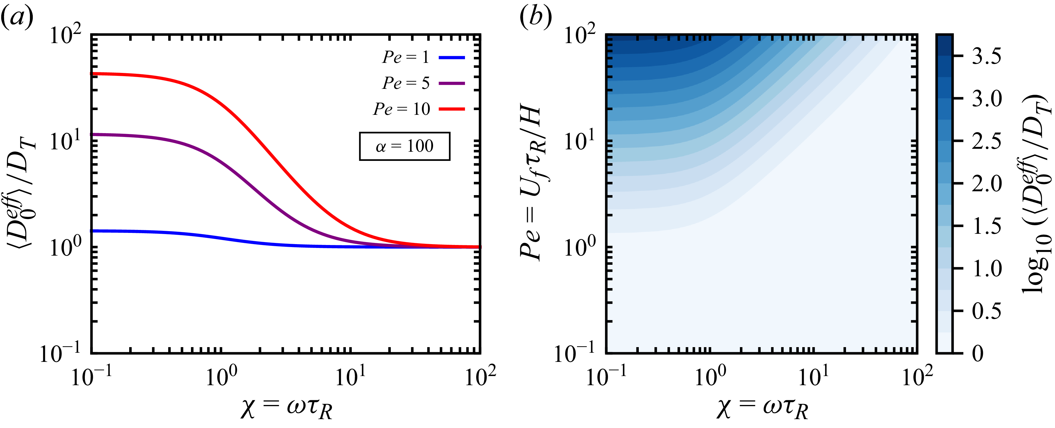


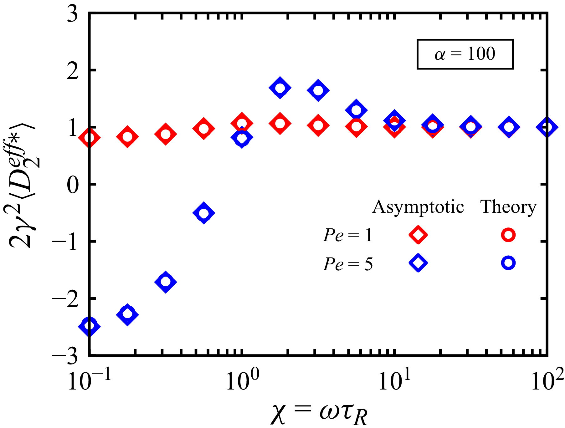


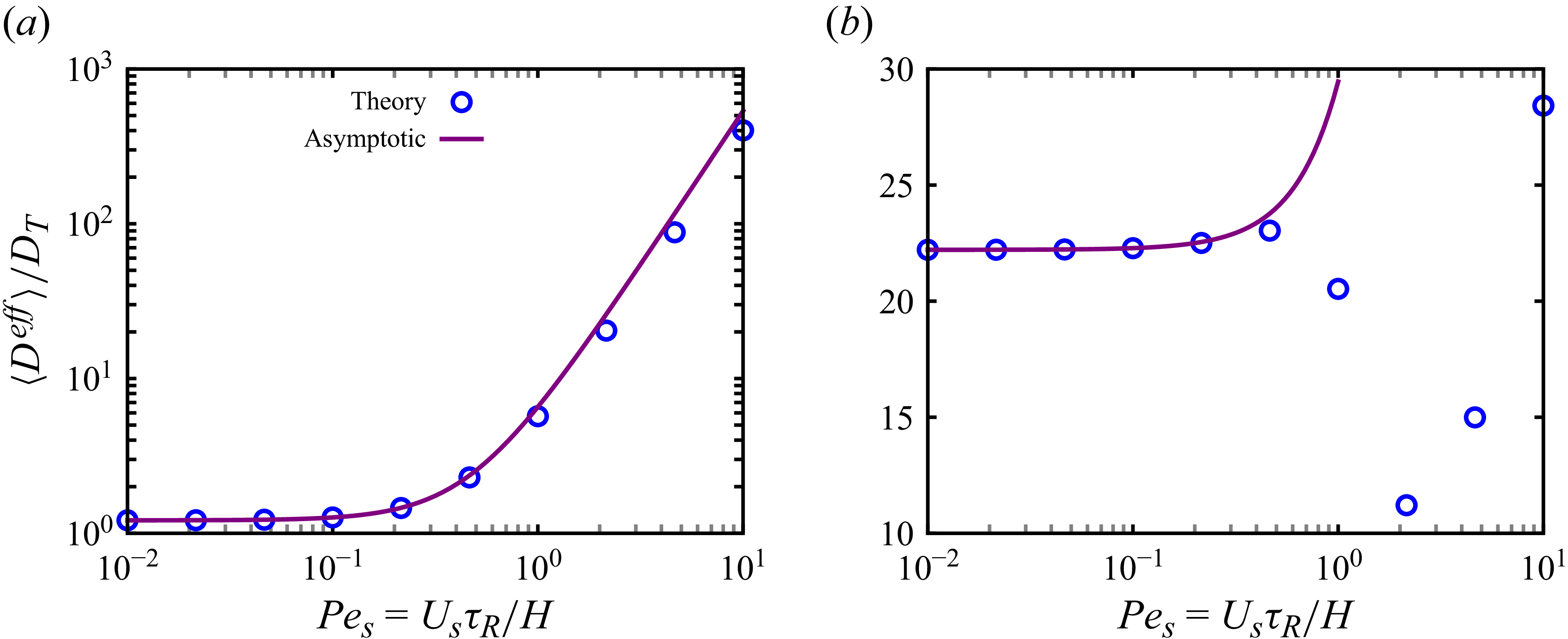


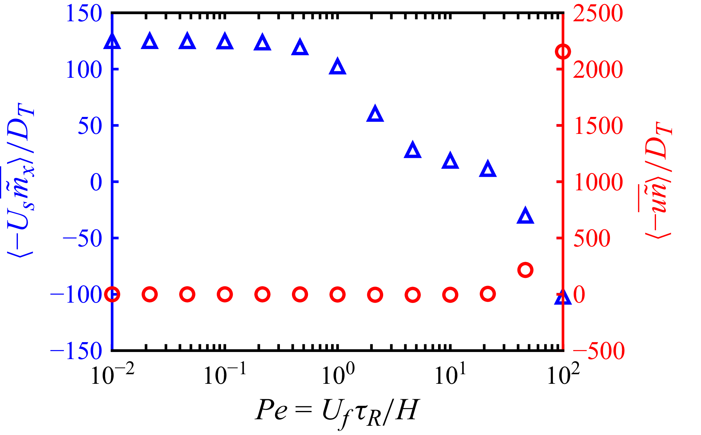


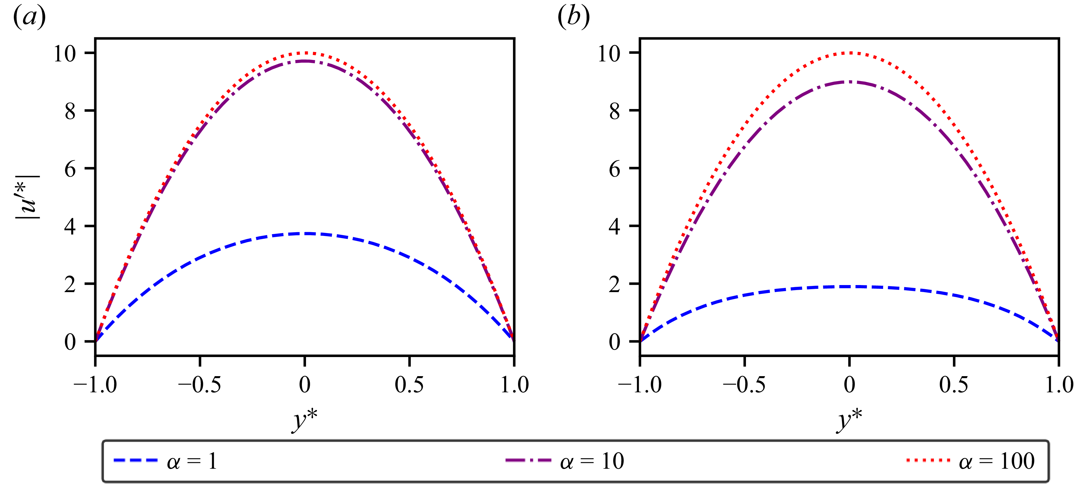


 Open access