





1. Introduction
Boiling is widely used in many applications, from coffee making to energy conversion, phase separation in chemical engineering and cooling of power electronics. The bubble dynamics at boiling has been actively studied since the 1950s by analysing sidewise shadowgraphy images. It was found that there are two distinct bubble growth regimes. Right after the nucleation, the bubble growth is controlled by its growing pressure (Tong & Tang Reference Tong and Tang2018) and the bubble radius is nearly linear in time. The growth is so fast that the inertia of the expelled liquid induces a downward-directed force that leads to the bubble `flattening’, hence, its hemispherical shape. This stage of growth is called inertial. At certain conditions (Snoeijer et al. Reference Snoeijer, Delon, Fermigier and Andreotti2006; Bureš & Sato Reference Bureš and Sato2021), the triple, liquid–vapour–heater contact line recedes slower than the bubble foot edge (figure 1), so a thin liquid layer is trapped between the heated wall and the interface of the bubble. This layer of liquid is known as the microlayer. It was indirectly observed for the first time by Moore & Mesler (Reference Moore and Mesler1961), whose micrometric homemade thermocouples measured high surface temperature variations with relatively long time periods, which could not be explained either by liquid advection or by evaporation in the contact line vicinity. Later, Torikai (Reference Torikai1967) successfully performed its direct observation from below. They used a transparent electro-conductive glass as a heated wall, and noticed a dry area smaller than the bubble foot, which confirmed the existence of a liquid layer below the bubble. Jawurek (Reference Jawurek1969) was the first to measure its thickness with laser interferometry (LI) at a few $\unicode{x03BC}$
m. The microlayer plays a crucial role, as its low thickness leads to high heat transfer from the wall to the fluid, thereby efficiently cooling down the wall and considerably (up to
$\unicode{x03BC}$
m. The microlayer plays a crucial role, as its low thickness leads to high heat transfer from the wall to the fluid, thereby efficiently cooling down the wall and considerably (up to $\sim$
50 %) contributing to the overall bubble growth (Myers et al. Reference Myers, Yerramilli, Hussey, Yee and Kim2005; Jung & Kim Reference Jung and Kim2014; Yabuki & Nakabeppu Reference Yabuki and Nakabeppu2014; Tecchio et al. Reference Tecchio2024a
).
$\sim$
50 %) contributing to the overall bubble growth (Myers et al. Reference Myers, Yerramilli, Hussey, Yee and Kim2005; Jung & Kim Reference Jung and Kim2014; Yabuki & Nakabeppu Reference Yabuki and Nakabeppu2014; Tecchio et al. Reference Tecchio2024a
).
The wettability of the wall, together with its natural heterogeneity and roughness can provide preferential places that act as the vapour bubble nucleation sites (Gallo et al. Reference Gallo, Magaletti, Georgoulas, Marengo, De Coninck and Casciola2023). From the experimental point of view, the main parameter dependent on all these surface properties is the wall superheating $\Delta T$
(i.e. the difference of the wall temperature
$\Delta T$
(i.e. the difference of the wall temperature $T_w$
and saturation temperature
$T_w$
and saturation temperature $T_{\textit{sat}}$
defined for the system pressure) required for the bubble nucleation. One calls it alternatively the nucleation barrier or the superheating of the nucleation site activation that results in the onset of nucleate boiling. For this reason, it is denoted
$T_{\textit{sat}}$
defined for the system pressure) required for the bubble nucleation. One calls it alternatively the nucleation barrier or the superheating of the nucleation site activation that results in the onset of nucleate boiling. For this reason, it is denoted $\Delta T_{\textit{ONB}}$
. It is important to mention that the nucleation is controlled by the wall superheating and not by the wall heat flux.
$\Delta T_{\textit{ONB}}$
. It is important to mention that the nucleation is controlled by the wall superheating and not by the wall heat flux.
To correctly target the growing bubble with cameras and sensors, the place of its nucleation should be fixed. The targeting is done either by localised heating or by creating a cavity that plays the role of an artificial nucleation site. This latter method was pioneered by Howell & Siegel (Reference Howell and Siegel1966). Since then it has become a common practice used at present by almost all research groups working on boiling (Qi & Klausner Reference Qi and Klausner2005; Hutter et al. Reference Hutter, Sanna, Karayiannis, Kenning, Nelson, Sefiane and Walton2013; Kangude & Srivastava Reference Kangude and Srivastava2020; Voulgaropoulos et al. Reference Voulgaropoulos, Aguiar, Markides and Bucci2022; Zupančič et al. Reference Zupančič, Gregorčič, Bucci, Wang, Matana Aguiar and Bucci2022). Shoji & Takagi (Reference Shoji and Takagi2001) investigated the boiling features of artificial cavities with conical, cylindrical and re-entrant geometries. They have found that cylindrical cavities provided the most stable ebullition cycles, which are the cycles of bubble growth and departure on the same site (Tong & Tang Reference Tong and Tang2018). Such a behaviour was also found numerically by Whiting et al. (Reference Whiting, van den Bergh, Theodorakis and Everts2024). They concluded that it resulted from the minimum bubble base radius prior to departure being constant and equal to the cavity radius, whereas this was not necessarily true for conical cavities.
The microlayer observation is difficult because, in addition to a small length scale, the time scale of the microlayer formation is of the order of several milliseconds for water at atmospheric pressure. Since the 1960s, the microlayer observation and measurement by two simultaneously applied experimental methods (typically, the sidewise shadowgraphy and observation or measurement from below) remained the state of the art for a long time. Jung & Kim (Reference Jung and Kim2014) were first to apply a triple observation by adding to the optical observations from the side and a simultaneous observation with an infra-red (IR) camera from below, i.e. by using IR thermography (IRT). This gave access to understanding of the spatial distribution of heat and mass transfer along the microlayer. The technique of LI has long been used for the measurements of the microlayer thickness. Tecchio et al. (Reference Tecchio, Zhang, Cariteau, Zalczer, Roca i Cabarrocas, Bulkin, Charliac, Vassant and Nikolayev2024c ) were first to apply the triple observation by replacing LI with white light interferometry (WLI).
Schematics of a single bubble growing on a heated wall. (a) Bubble macroscopic view. (b) Microlayer.

The model of Cooper & Lloyd (Reference Cooper and Lloyd1969) (cf. § 3.6 below) dominated theoretical ideas about the microlayer’s formation until recently. It was based on the scaling of the microlayer thickness with that of the viscous boundary layer. It thus resulted in a monotonic growth of the microlayer thickness in agreement with its early experimental studies (Jawurek Reference Jawurek1969; Koffman & Plesset Reference Koffman and Plesset1983; Yabuki & Nakabeppu Reference Yabuki and Nakabeppu2014). Such a picture was widely accepted by the scientific community until Chen, Haginiwa & Utaka (Reference Chen, Haginiwa and Utaka2017) discovered that the microlayer can have a bumped shape also observed in the forthcoming studies of other groups (Jung & Kim Reference Jung and Kim2018; Narayan & Srivastava Reference Narayan and Srivastava2021; Tecchio et al. Reference Tecchio, Zhang, Cariteau, Zalczer, Roca i Cabarrocas, Bulkin, Charliac, Vassant and Nikolayev2024c ).
Following the initial idea of Zijl & Moalem-Maron (Reference Zijl and Moalem-Maron1978), it was shown experimentally (Tecchio et al. Reference Tecchio, Zhang, Cariteau, Zalczer, Roca i Cabarrocas, Bulkin, Charliac, Vassant and Nikolayev2024c
) that the formation of microlayer is analogous to the deposition of a thin liquid film on a flat plate that one pulls out vertically from a pool of liquid with a speed $U_b$
. This phenomenon was first modelled by Landau & Levich (Reference Landau and Levich1942), who demonstrated that the thickness of such a film is defined by the interplay of the viscous and surface tension forces. According to their theory developed in the asymptotic limit
$U_b$
. This phenomenon was first modelled by Landau & Levich (Reference Landau and Levich1942), who demonstrated that the thickness of such a film is defined by the interplay of the viscous and surface tension forces. According to their theory developed in the asymptotic limit $ \textit{Ca}_b\ll 1$
 \begin{align} \delta _0=1.34r_c \textit{Ca}_b^{2/3}, \end{align}
where the capillary number is $ \textit{Ca}_b=\mu U_b/\sigma$
;
$ \textit{Ca}_b=\mu U_b/\sigma$
; $\mu$
and
$\mu$
and $\sigma$
stand for the dynamic viscosity and the surface tension, respectively and
$\sigma$
stand for the dynamic viscosity and the surface tension, respectively and $r_c$
is the radius of liquid surface curvature near the plate. The same formula was rederived by Bretherton (Reference Bretherton1961) for the case of a film deposited by the receding meniscus inside a capillary. The microlayer is left behind the bubble foot edge of the curvature
$r_c$
is the radius of liquid surface curvature near the plate. The same formula was rederived by Bretherton (Reference Bretherton1961) for the case of a film deposited by the receding meniscus inside a capillary. The microlayer is left behind the bubble foot edge of the curvature $r_c^{-1}$
(figure 1
b) receding with the speed
$r_c^{-1}$
(figure 1
b) receding with the speed $U_b=\dot r_b$
that represents the speed of bubble lateral growth (dot indicates the time derivative). This means that the microlayer thickness is controlled only by the viscous and surface tension forces while the overall bubble shape is controlled by the interplay of the liquid inertia and surface tension during the microlayer formation.
$U_b=\dot r_b$
that represents the speed of bubble lateral growth (dot indicates the time derivative). This means that the microlayer thickness is controlled only by the viscous and surface tension forces while the overall bubble shape is controlled by the interplay of the liquid inertia and surface tension during the microlayer formation.
Two last columns of table 1 show the maximum values $ \textit{Ca}_b^{\textit{max}}$
and
$ \textit{Ca}_b^{\textit{max}}$
and $ \textit{Re}^{\textit{max}}$
of the capillary and the Reynolds microlayer numbers
$ \textit{Re}^{\textit{max}}$
of the capillary and the Reynolds microlayer numbers $Re=U_b\rho_l \delta_0/\mu$
, where
$Re=U_b\rho_l \delta_0/\mu$
, where $\rho_l$
stands for the liquid density. They use the maximum
$\rho_l$
stands for the liquid density. They use the maximum $U_b$
and
$U_b$
and $\delta _0$
encountered during the computation of microlayer parameters in § 3.5. The values of
$\delta _0$
encountered during the computation of microlayer parameters in § 3.5. The values of $ \textit{Re}^{\textit{max}}\simeq 20$
show some contribution of inertia at the bubble foot edge. However, as the velocity decreases exponentially with decreasing
$ \textit{Re}^{\textit{max}}\simeq 20$
show some contribution of inertia at the bubble foot edge. However, as the velocity decreases exponentially with decreasing $r$
according to Bretherton (Reference Bretherton1961), the lubrication approximation should apply to the microlayer description.
$r$
according to Bretherton (Reference Bretherton1961), the lubrication approximation should apply to the microlayer description.
List of different experiments. Cases A–C correspond to different boiling surfaces. Cases A and C refer to our previous works (Tecchio et al. Reference Tecchio, Regoli, Cariteau, Zalczer, Roca I Cabarrocas, Bulkin, Charliac, Vassant and Nikolayev2024b
,
Reference Tecchio, Zhang, Cariteau, Zalczer, Roca i Cabarrocas, Bulkin, Charliac, Vassant and Nikolayevc
). The maximum values of $ \textit{Ca}_b$
and
$ \textit{Ca}_b$
and $ \textit{Re}$
are not shown for 103 and 107
$ \textit{Re}$
are not shown for 103 and 107 $\textrm {kW}\,\textrm {m}^{-2}$
because the WLI fringes do not have high enough optical contrast to post-process the images.
$\textrm {kW}\,\textrm {m}^{-2}$
because the WLI fringes do not have high enough optical contrast to post-process the images.

The initial microlayer thickness $\delta _0(r)$
is that right after microlayer formation. One should note that the
$\delta _0(r)$
is that right after microlayer formation. One should note that the $r_c$
value is much smaller than the bubble radius
$r_c$
value is much smaller than the bubble radius $r_b$
shown in figure 1(a). This high curvature occurs in a transition zone between the nearly flat microlayer and the remaining nearly hemispherical part of the bubble interface. While
$r_b$
shown in figure 1(a). This high curvature occurs in a transition zone between the nearly flat microlayer and the remaining nearly hemispherical part of the bubble interface. While $ \textit{Ca}_b$
is accessible experimentally, it is unfortunately impossible to measure
$ \textit{Ca}_b$
is accessible experimentally, it is unfortunately impossible to measure $r_c$
by optical shadowgraphy because of the mirage effect that deforms the bubble image near the heated wall (Cooper Reference Cooper1983). It was previously shown (Tecchio et al. Reference Tecchio, Zhang, Cariteau, Zalczer, Roca i Cabarrocas, Bulkin, Charliac, Vassant and Nikolayev2024c
) that an assumption of a constant
$r_c$
by optical shadowgraphy because of the mirage effect that deforms the bubble image near the heated wall (Cooper Reference Cooper1983). It was previously shown (Tecchio et al. Reference Tecchio, Zhang, Cariteau, Zalczer, Roca i Cabarrocas, Bulkin, Charliac, Vassant and Nikolayev2024c
) that an assumption of a constant $r_c/r_b$
ratio throughout the inertial stage gives results coherent with experiment and numerical simulation.
$r_c/r_b$
ratio throughout the inertial stage gives results coherent with experiment and numerical simulation.
In this work, we aim to study in depth the bubble dynamics in saturated pool boiling experiments of water at atmospheric pressure by focusing on the microlayer formation. For this purpose, we investigate the single-bubble boiling regime (where one bubble grows without any influence from the others) with fast, synchronised and highly spatially resolved shadowgraphy coupled with WLI and IRT. Artificial nucleation centres are used as a means to produce different bubble growth rates by controlling the nucleation barrier, which allows us to investigate the initial microlayer thickness over a wide range of $ \textit{Ca}_b$
. We develop a method to recover
$ \textit{Ca}_b$
. We develop a method to recover $r_c$
from the experimental data and discuss the initial microlayer thickness for different cases; our data are finally compared with existing phenomenological models.
$r_c$
from the experimental data and discuss the initial microlayer thickness for different cases; our data are finally compared with existing phenomenological models.
2. Experimental
A schematic of the experimental installation is presented in figure 2. The boiling cell consists of a water pool surrounded by a temperature-regulated jacket. The water pool is at atmospheric pressure and saturation temperature. The ultra-pure water (Merck Millipore) with 2 ppb total organic carbon and 18.2 $\textrm {M} \Omega \,\textrm {cm}$
resistivity, additionally purified in situ by the Milli-Q IQ 7003 installation, was used in all the experiments. The water was boiled for several hours prior to the experiments to eliminate the non-condensable gases.
$\textrm {M} \Omega \,\textrm {cm}$
resistivity, additionally purified in situ by the Milli-Q IQ 7003 installation, was used in all the experiments. The water was boiled for several hours prior to the experiments to eliminate the non-condensable gases.
Schematics of the experimental set-up and experimentally obtained images. The sidewise shadowgraphy gives the overall bubble shape and its radius $r_b(t)$
(image (a)). The white-light interferometry (image (b)) gives the contact line radius
$r_b(t)$
(image (a)). The white-light interferometry (image (b)) gives the contact line radius $r_{cl}(t)$
, the microlayer edge position
$r_{cl}(t)$
, the microlayer edge position $r_{\mu }(t)$
and the microlayer thickness
$r_{\mu }(t)$
and the microlayer thickness $\delta (r,t)$
. The mirror mode (image (c)) is used to check whether a bubble is axisymmetric and to align the slit with the bubble centre. The IRT gives the wall temperature distribution
$\delta (r,t)$
. The mirror mode (image (c)) is used to check whether a bubble is axisymmetric and to align the slit with the bubble centre. The IRT gives the wall temperature distribution $T_w(x,y,t)$
(image (d)).
$T_w(x,y,t)$
(image (d)).

2.1. Boiling surfaces
The boiling surfaces consist of a 3 mm-thick magnesium fluoride (MgF $_2$
) porthole on which a 950 nm-thick indium-tin oxide (ITO) film is deposited by using a radio-frequency magnetron sputtering system. The MgF
$_2$
) porthole on which a 950 nm-thick indium-tin oxide (ITO) film is deposited by using a radio-frequency magnetron sputtering system. The MgF $_2$
is transparent to both visible and IR waves, whereas ITO is transparent in visible but opaque in the IR wavelength range. To ensure the growth of a single bubble at a time, the ITO film is heated up locally with an IR continuous laser (wavelength of 1.2
$_2$
is transparent to both visible and IR waves, whereas ITO is transparent in visible but opaque in the IR wavelength range. To ensure the growth of a single bubble at a time, the ITO film is heated up locally with an IR continuous laser (wavelength of 1.2 $\unicode{x03BC}$
m). The laser beam has a Gaussian-like profile. The applied wall heat flux
$\unicode{x03BC}$
m). The laser beam has a Gaussian-like profile. The applied wall heat flux $q_a''$
is calculated as described in Appendix A. The heat flux can be varied among different experimental cases (see table 1) by changing the beam diameter and the laser power.
$q_a''$
is calculated as described in Appendix A. The heat flux can be varied among different experimental cases (see table 1) by changing the beam diameter and the laser power.
This study compares the data obtained from three different boiling surfaces; table 1 summarises their parameters. Case A refers to our previous work (Tecchio et al. Reference Tecchio2024a
,Reference Tecchio, Zhang, Cariteau, Zalczer, Roca i Cabarrocas, Bulkin, Charliac, Vassant and Nikolayev
c
), in which no artificial cavity was created on a boiling surface. The optically smooth ITO surface (its roughness was $\simeq {10}\,\textrm {nm}$
) had a `natural’ point defect that served as a nucleation site for the bubbles (figure 3
a).
$\simeq {10}\,\textrm {nm}$
) had a `natural’ point defect that served as a nucleation site for the bubbles (figure 3
a).
In cases B and C (the latter refers to the work of Tecchio et al. Reference Tecchio, Regoli, Cariteau, Zalczer, Roca I Cabarrocas, Bulkin, Charliac, Vassant and Nikolayev2024b
), the bubble nucleates on an artificial cavity with a depth $h$
approximately twice larger than its upper diameter
$h$
approximately twice larger than its upper diameter $d$
(figure 3
c). The cavity is fabricated on the MgF
$d$
(figure 3
c). The cavity is fabricated on the MgF $_2$
window by the focused ion beam (FIB) technology prior to the ITO deposition. The cavity is slightly conical, with the slant angle
$_2$
window by the focused ion beam (FIB) technology prior to the ITO deposition. The cavity is slightly conical, with the slant angle $\beta$
(figure 3
b). However, it is quite small, so the cavity shape is close to cylindrical. The cavity parameters are provided in table 1.
$\beta$
(figure 3
b). However, it is quite small, so the cavity shape is close to cylindrical. The cavity parameters are provided in table 1.
The precise position of a cavity on the ITO is known a priori only approximately. To locate it precisely, one displaces the IR laser spot that is easily visible on the IRT image along the surface with the micrometric translation stage. Once the laser beam centre is close enough to the cavity, bubble nucleation occurs. Next, the laser beam is centred on the cavity. The natural defect in case A was localised with a similar procedure.
Schematics of the boiling surfaces. (a) No artificial cavity (case A of table 1). (b) Artificial cavity, cases B and C (the cavity is not to scale). (c) Slanted scanning electron microscopy image of the cavity. The substrate cross-cut is performed with FIB. The lengths $h$
and
$h$
and $d$
stand for the depth and the mouth diameter of a cavity, respectively.
$d$
stand for the depth and the mouth diameter of a cavity, respectively.

2.2. Measurement techniques
The measurement techniques employed in this study are described extensively in our previous studies (Tecchio et al. Reference Tecchio, Regoli, Cariteau, Zalczer, Roca I Cabarrocas, Bulkin, Charliac, Vassant and Nikolayev2024b
,
Reference Tecchio, Zhang, Cariteau, Zalczer, Roca i Cabarrocas, Bulkin, Charliac, Vassant and Nikolayevc
). Only a concise description is given here. The bubble macroscopic shape and its radius $r_b(t)$
(figure 2
a) are obtained by sidewise shadowgraphy with a spatial resolution of 32
$r_b(t)$
(figure 2
a) are obtained by sidewise shadowgraphy with a spatial resolution of 32 $\unicode{x03BC}$
m px−1 for case A and 9
$\unicode{x03BC}$
m px−1 for case A and 9 $\unicode{x03BC}$
m px−1 for cases B and C thanks to a better optical set-up.
$\unicode{x03BC}$
m px−1 for cases B and C thanks to a better optical set-up.
The microlayer thickness is measured by WLI that has many advantages over LI. (i) The WLI is much more precise: for each $r$
, the amount of data is comparable to the vertical image size in pixels in WLI, while it is one in LI (single laser wavelength). (ii) The spatial resolution of WLI is much larger. In LI, the distance between the measurement points is limited by the distance between the fringes. In WLI, it is limited only by the resolution of the optical system. (iii) The LI relies on the fringe number. When the vapour-liquid (V-L) interface slope is high (typically, near the edge of the measured
$r$
, the amount of data is comparable to the vertical image size in pixels in WLI, while it is one in LI (single laser wavelength). (ii) The spatial resolution of WLI is much larger. In LI, the distance between the measurement points is limited by the distance between the fringes. In WLI, it is limited only by the resolution of the optical system. (iii) The LI relies on the fringe number. When the vapour-liquid (V-L) interface slope is high (typically, near the edge of the measured $r$
interval, e.g. near the contact line) the fringes become dense and some of them can be lost because of insufficient resolution of the optical system. So the LI results on a microlayer might be given only within a constant offset thickness. The WLI is deprived of such an uncertainty and always gives the absolute thickness value. (iv) The general shape of the microlayer corresponds to the WLI fringe shape (figure 2
b) so the microlayer bump can be seen during the experiment without any processing.
$r$
interval, e.g. near the contact line) the fringes become dense and some of them can be lost because of insufficient resolution of the optical system. So the LI results on a microlayer might be given only within a constant offset thickness. The WLI is deprived of such an uncertainty and always gives the absolute thickness value. (iv) The general shape of the microlayer corresponds to the WLI fringe shape (figure 2
b) so the microlayer bump can be seen during the experiment without any processing.
The WLI is set up as follows. A LED light source produces a collimated beam of white light that is shone towards the bubble from below perpendicularly to the wall. The reflected light is directed with a visible light beam splitter towards a spectrometer. A slit located at the entrance of the spectrometer defines the scanning line, along which the microlayer profile is measured. The set-up is adjusted in such a way that the scanning line passes through the bubble centre. In the spectrometer, the light is dispersed by a diffraction grating; a fast camera records the spectral fringe map (figure 2
b). It results from the interference of the rays reflected from the interfaces between MgF $_2$
/ITO, ITO/microlayer and microlayer/vapour. In figure 2(b), the ordinate corresponds to the wavelength
$_2$
/ITO, ITO/microlayer and microlayer/vapour. In figure 2(b), the ordinate corresponds to the wavelength $\lambda$
and the abscissa to the physical position along the scanning line. The diffraction grating can be replaced by a mirror to observe the bubble from below (figure 2
c). These images serve to verify that, in all of the cases, the bubbles are nearly cylindrically symmetric thanks to a good quality of ITO (sufficiently smooth and chemically homogeneous). This allows us to associate the coordinate along the scanning line with the radial coordinate
$\lambda$
and the abscissa to the physical position along the scanning line. The diffraction grating can be replaced by a mirror to observe the bubble from below (figure 2
c). These images serve to verify that, in all of the cases, the bubbles are nearly cylindrically symmetric thanks to a good quality of ITO (sufficiently smooth and chemically homogeneous). This allows us to associate the coordinate along the scanning line with the radial coordinate $r$
. The microlayer thickness profile
$r$
. The microlayer thickness profile $\delta (r,t)$
is determined by comparing the experimental spectral intensity with the two-beam interference model (Tecchio Reference Tecchio2022).
$\delta (r,t)$
is determined by comparing the experimental spectral intensity with the two-beam interference model (Tecchio Reference Tecchio2022).
From figure 2(b), one can also obtain the dry spot (contact line) radius $r_{cl}$
as the radius where the optical contrast changes sharply due to a difference of reflectivity (given by the Fresnel coefficients) from the interfaces of ITO with the vapour and the liquid that have different refraction indices. From the optical analysis, one can also deduce the microlayer edge position
$r_{cl}$
as the radius where the optical contrast changes sharply due to a difference of reflectivity (given by the Fresnel coefficients) from the interfaces of ITO with the vapour and the liquid that have different refraction indices. From the optical analysis, one can also deduce the microlayer edge position $r_{\mu }$
as a maximal radial coordinate, within which the interference fringes appear. Even if the optical resolution is not high enough to distinguish them (which is often the case near the microlayer edge), they lead to a brighter image than the bulk liquid.
$r_{\mu }$
as a maximal radial coordinate, within which the interference fringes appear. Even if the optical resolution is not high enough to distinguish them (which is often the case near the microlayer edge), they lead to a brighter image than the bulk liquid.
The wavelength bandwidth of WLI is 444.6–587.7 nm, and the spectral resolution is 0.21 nm px–1. The WLI spatial resolution along $r$
is 14
$r$
is 14 $\unicode{x03BC}$
m px–1 for case A and 7.9
$\unicode{x03BC}$
m px–1 for case A and 7.9 $\unicode{x03BC}$
m px–1 for cases B, C thanks to a camera with a smaller pixel size. The spatial resolution defines the maximum measurable slope of the V-L interface (Tecchio et al. Reference Tecchio, Zhang, Cariteau, Zalczer, Roca i Cabarrocas, Bulkin, Charliac, Vassant and Nikolayev2024c
). The maximal slopes at
$\unicode{x03BC}$
m px–1 for cases B, C thanks to a camera with a smaller pixel size. The spatial resolution defines the maximum measurable slope of the V-L interface (Tecchio et al. Reference Tecchio, Zhang, Cariteau, Zalczer, Roca i Cabarrocas, Bulkin, Charliac, Vassant and Nikolayev2024c
). The maximal slopes at $\lambda ={500}\,\textrm {nm}$
are 0.38
$\lambda ={500}\,\textrm {nm}$
are 0.38 $^\circ$
for case A and 0.76
$^\circ$
for case A and 0.76 $^\circ$
for cases B, C.
$^\circ$
for cases B, C.
The IRT is used to measure the temporal evolution of the wall temperature distribution $T_w(x,y,t)$
in the Cartesian reference frame (
$T_w(x,y,t)$
in the Cartesian reference frame ( $x,y$
) (figure 2
d). We use a homemade multilayer visible–IR light beam splitter (transparent to visible but reflective to IR) positioned between the boiling cell and the visible light beam splitter to reflect the IR light emitted by the ITO. The reflected IR radiation is captured by a fast IR camera in the range 3–5
$x,y$
) (figure 2
d). We use a homemade multilayer visible–IR light beam splitter (transparent to visible but reflective to IR) positioned between the boiling cell and the visible light beam splitter to reflect the IR light emitted by the ITO. The reflected IR radiation is captured by a fast IR camera in the range 3–5 $\unicode{x03BC}$
m. The recorded intensity is then related to temperature using a pixel-wise calibration (Schweikert, Sielaff & Stephan Reference Schweikert, Sielaff and Stephan2021). A resistance temperature detector (RTD in figure 2) measures the water pool temperature near the boiling surface. The temperature measurements for the calibration are taken with the liquid pool at thermally homogeneous conditions. The spatial resolution of the IR camera is 84
$\unicode{x03BC}$
m. The recorded intensity is then related to temperature using a pixel-wise calibration (Schweikert, Sielaff & Stephan Reference Schweikert, Sielaff and Stephan2021). A resistance temperature detector (RTD in figure 2) measures the water pool temperature near the boiling surface. The temperature measurements for the calibration are taken with the liquid pool at thermally homogeneous conditions. The spatial resolution of the IR camera is 84 $\unicode{x03BC}$
m px–1 for cases A and C, and 100
$\unicode{x03BC}$
m px–1 for cases A and C, and 100 $\unicode{x03BC}$
m px–1 for case B.
$\unicode{x03BC}$
m px–1 for case B.
All optical observations are recorded synchronously at 4000 frames per second. Both the calibration and validation of WLI and IRT are described by Tecchio (Reference Tecchio2022) and the measurement uncertainties are provided in table 2.
Measurement uncertainties.

Wall superheating $\Delta T_0$
measured at the nucleation site location as a function of time for the cases listed in table 1. The case B curves are given for
$\Delta T_0$
measured at the nucleation site location as a function of time for the cases listed in table 1. The case B curves are given for $q_a''=$
80.7
$q_a''=$
80.7 $\,\textrm {kW}\,\textrm {m}^{-2}$
. The time
$\,\textrm {kW}\,\textrm {m}^{-2}$
. The time $t$
in figures 4(b–d) is counted from the bubble inception. (a) Long-time evolution. The respective
$t$
in figures 4(b–d) is counted from the bubble inception. (a) Long-time evolution. The respective $\Delta T_{\textit{ONB}}$
values are indicated to the right of each curve in K. (b) Evolution during the bubble growth time for case A (Tecchio et al. Reference Tecchio2024a
). (c) Evolution during the bubble growth time for case B. (d) Evolution during the bubble growth time for case C (Tecchio et al. Reference Tecchio, Regoli, Cariteau, Zalczer, Roca I Cabarrocas, Bulkin, Charliac, Vassant and Nikolayev2024b
).
$\Delta T_{\textit{ONB}}$
values are indicated to the right of each curve in K. (b) Evolution during the bubble growth time for case A (Tecchio et al. Reference Tecchio2024a
). (c) Evolution during the bubble growth time for case B. (d) Evolution during the bubble growth time for case C (Tecchio et al. Reference Tecchio, Regoli, Cariteau, Zalczer, Roca I Cabarrocas, Bulkin, Charliac, Vassant and Nikolayev2024b
).

3. Results and discussion
Table 1 shows the experimental cases that correspond to different boiling surfaces described above. The surfaces A and C were studied at a fixed heat power. Experiments in case B were performed for several heating power values corresponding to the reference heat fluxes 64–107 kW m− $^2$
.
$^2$
.
3.1. Ebullition cycles
Figure 4 depicts the temporal evolution of the wall superheating at the nucleation site location denoted $\Delta T_0$
. Figure 4(a) shows consecutive ebullition cycles. They follow a periodic pattern with a period
$\Delta T_0$
. Figure 4(a) shows consecutive ebullition cycles. They follow a periodic pattern with a period $t_c$
, which is a cycle duration. The high repeatability occurs thanks to a high quality of the boiling surface causing the nucleation on the single nucleation site, thus avoiding thermal and hydrodynamic interactions with other bubbles. This means that one ebullition cycle is sufficient to be studied as it is representative of the whole dynamics.
$t_c$
, which is a cycle duration. The high repeatability occurs thanks to a high quality of the boiling surface causing the nucleation on the single nucleation site, thus avoiding thermal and hydrodynamic interactions with other bubbles. This means that one ebullition cycle is sufficient to be studied as it is representative of the whole dynamics.
One can see that $\Delta T_0$
periodically attains its maximum at a specific superheating. The maximum is reached at the bubble nucleation, where a sharp temperature drop occurs due to a consumption of energy needed to compensate the latent heat of vaporisation. The maximum superheating corresponds to
$\Delta T_0$
periodically attains its maximum at a specific superheating. The maximum is reached at the bubble nucleation, where a sharp temperature drop occurs due to a consumption of energy needed to compensate the latent heat of vaporisation. The maximum superheating corresponds to $\Delta T_{\textit{ONB}}$
. One can see (table 1) that it depends on the boiling surface and is smaller by factors
$\Delta T_{\textit{ONB}}$
. One can see (table 1) that it depends on the boiling surface and is smaller by factors $2$
and
$2$
and $3.4$
for cases B and C, respectively, in comparison with case A. Such a behaviour is non-monotonic with respect to the cavity diameter, which suggests that the relevant nucleation length scale is different (probably corresponding to the roughness inside the cavity). It is well known that controlling nucleation by the surface geometry is extremely difficult (Qi & Klausner Reference Qi and Klausner2005). Therefore,
$3.4$
for cases B and C, respectively, in comparison with case A. Such a behaviour is non-monotonic with respect to the cavity diameter, which suggests that the relevant nucleation length scale is different (probably corresponding to the roughness inside the cavity). It is well known that controlling nucleation by the surface geometry is extremely difficult (Qi & Klausner Reference Qi and Klausner2005). Therefore, $\Delta T_{\textit{ONB}}$
is used hereafter as a main parameter describing the boiling surface.
$\Delta T_{\textit{ONB}}$
is used hereafter as a main parameter describing the boiling surface.
The detailed analysis of an ebullition cycle shows that it consists of the time $t_d$
of the bubble residence on the heater and waiting time
$t_d$
of the bubble residence on the heater and waiting time $t_w\gg t_d$
until next nucleation event, i.e.
$t_w\gg t_d$
until next nucleation event, i.e. $t_c=t_d+t_w$
(cf. figure 4). The
$t_c=t_d+t_w$
(cf. figure 4). The $\Delta T_0$
evolution during the residence is analysed in figure 4(b–d). From now on, we set the time origin
$\Delta T_0$
evolution during the residence is analysed in figure 4(b–d). From now on, we set the time origin $t=0$
at the bubble inception (nucleation) to describe a single ebullition cycle. The time evolution of
$t=0$
at the bubble inception (nucleation) to describe a single ebullition cycle. The time evolution of $\Delta T_0$
is qualitatively similar for all three cases. Once the nucleation occurs at
$\Delta T_0$
is qualitatively similar for all three cases. Once the nucleation occurs at $\Delta T_0=\Delta T_{\textit{ONB}}$
, the temperature decreases because of a strong consumption of the latent heat at the fast inertial growth stage. Next, the temperature increases due to formation and growth of a dry spot at the nucleation site because the heat transfer to the vapour is very small. Although a dry spot forms immediately (cf. figure 8 below),
$\Delta T_0=\Delta T_{\textit{ONB}}$
, the temperature decreases because of a strong consumption of the latent heat at the fast inertial growth stage. Next, the temperature increases due to formation and growth of a dry spot at the nucleation site because the heat transfer to the vapour is very small. Although a dry spot forms immediately (cf. figure 8 below), $\Delta T_0$
continues to decrease for some time. This can be attributed to a high evaporation in the contact line vicinity (Nikolayev Reference Nikolayev2022) that drains the energy stored in the wall. Next, the contact line evaporation manifests itself once again, when the advancing contact line approaches the bubble centre (just before the bubble departure under the action of buoyancy) causing a
$\Delta T_0$
continues to decrease for some time. This can be attributed to a high evaporation in the contact line vicinity (Nikolayev Reference Nikolayev2022) that drains the energy stored in the wall. Next, the contact line evaporation manifests itself once again, when the advancing contact line approaches the bubble centre (just before the bubble departure under the action of buoyancy) causing a $\Delta T_0$
decrease. It becomes more pronounced after the bubble departure due to the wall quenching by convection from the bulk colder liquid (Wei et al. Reference Wei, Bois, Pandey and Nikolayev2025).
$\Delta T_0$
decrease. It becomes more pronounced after the bubble departure due to the wall quenching by convection from the bulk colder liquid (Wei et al. Reference Wei, Bois, Pandey and Nikolayev2025).
In case A, the $\Delta T_0$
drop after nucleation is much sharper than in cases B and C because of a higher cooling rate due to evaporation, whose rate increases with
$\Delta T_0$
drop after nucleation is much sharper than in cases B and C because of a higher cooling rate due to evaporation, whose rate increases with $\Delta T_{\textit{ONB}}$
. After the initial decrease,
$\Delta T_{\textit{ONB}}$
. After the initial decrease, $\Delta T_0$
increases because of the dry spot growth, which is also faster at a higher superheating (Zhang & Nikolayev Reference Zhang and Nikolayev2022). The
$\Delta T_0$
increases because of the dry spot growth, which is also faster at a higher superheating (Zhang & Nikolayev Reference Zhang and Nikolayev2022). The $\Delta T_0$
decrease just before the bubble departure is sharper too because the contact line cooling effect increases with the local superheating.
$\Delta T_0$
decrease just before the bubble departure is sharper too because the contact line cooling effect increases with the local superheating.
3.2. Effect of heat flux on the bubble growth
Before considering in detail the effect of $\Delta T_{\textit{ONB}}$
on the bubble dynamics, we discuss the effect of the applied heat flux
$\Delta T_{\textit{ONB}}$
on the bubble dynamics, we discuss the effect of the applied heat flux $q_a''$
. It is controlled by both the beam diameter
$q_a''$
. It is controlled by both the beam diameter $D$
and the power of the IR laser
$D$
and the power of the IR laser $q_{las}$
that can be varied independently and significantly (Appendix A). To evaluate the heat flux effect, we compare the bubble evolution observed at a fixed
$q_{las}$
that can be varied independently and significantly (Appendix A). To evaluate the heat flux effect, we compare the bubble evolution observed at a fixed $D$
and varying
$D$
and varying $q_{las}$
. This is done for the boiling surface of case B, i.e. for the original data obtained in this work.
$q_{las}$
. This is done for the boiling surface of case B, i.e. for the original data obtained in this work.
Impact of $q_a''$
on (a)
$q_a''$
on (a) $t_d$
, (b)
$t_d$
, (b) $\Delta T_{\textit{ONB}}$
and (c)
$\Delta T_{\textit{ONB}}$
and (c) $t_w$
for case B. The lines are the eye guides.
$t_w$
for case B. The lines are the eye guides.

Time evolution of characteristic bubble radii for case B. The curve parameter is $q_a''$
in
$q_a''$
in $\,\textrm {kW}\,\textrm {m}^{-2}$
. The data are plotted from the bubble inception (
$\,\textrm {kW}\,\textrm {m}^{-2}$
. The data are plotted from the bubble inception ( $t=0$
) up to its departure from the wall. (a) Bubble radius
$t=0$
) up to its departure from the wall. (a) Bubble radius $r_b$
. (b) Microlayer edge position
$r_b$
. (b) Microlayer edge position $r_\mu$
. (c) Contact line position
$r_\mu$
. (c) Contact line position $r_{cl}$
.
$r_{cl}$
.

The influence of the applied heat flux $q_a''$
on
$q_a''$
on $\Delta T_{\textit{ONB}}$
, the bubble growth time
$\Delta T_{\textit{ONB}}$
, the bubble growth time $t_d$
and the waiting time
$t_d$
and the waiting time $t_w$
is analysed in figure 5, where the error bars of
$t_w$
is analysed in figure 5, where the error bars of $t_d$
and
$t_d$
and $t_w$
are computed as a standard deviation over at least 7 ebullition cycles, and those for
$t_w$
are computed as a standard deviation over at least 7 ebullition cycles, and those for $\Delta T_{\textit{ONB}}$
are the measurement uncertainties (these
$\Delta T_{\textit{ONB}}$
are the measurement uncertainties (these $\Delta T_{\textit{ONB}}$
values are also shown in table 1). Here,
$\Delta T_{\textit{ONB}}$
values are also shown in table 1). Here, $\Delta T_{\textit{ONB}}$
stays nearly constant, regardless of
$\Delta T_{\textit{ONB}}$
stays nearly constant, regardless of $q_a''$
. This indicates that the nucleation depends on the wall temperature but not on the wall heat flux, which is coherent both with the classical nucleation theory (Tong & Tang Reference Tong and Tang2018) and the contemporary picture of nucleation (Gallo et al. Reference Gallo, Magaletti, Georgoulas, Marengo, De Coninck and Casciola2023). No significant variation of the departure time
$q_a''$
. This indicates that the nucleation depends on the wall temperature but not on the wall heat flux, which is coherent both with the classical nucleation theory (Tong & Tang Reference Tong and Tang2018) and the contemporary picture of nucleation (Gallo et al. Reference Gallo, Magaletti, Georgoulas, Marengo, De Coninck and Casciola2023). No significant variation of the departure time $t_d$
is detected either. However,
$t_d$
is detected either. However, $t_w$
decreases with increasing
$t_w$
decreases with increasing $q_a''$
. This occurs because
$q_a''$
. This occurs because $\Delta T_{\textit{ONB}}$
is reached faster (the substrate is heated faster) when a higher heat flux is applied.
$\Delta T_{\textit{ONB}}$
is reached faster (the substrate is heated faster) when a higher heat flux is applied.
It should be mentioned that the working interval of $q_a''$
is strongly limited for each boiling surface. On one hand, a certain flux value is necessary to achieve
$q_a''$
is strongly limited for each boiling surface. On one hand, a certain flux value is necessary to achieve $\Delta T_{\textit{ONB}}$
. For a smaller flux, the wall superheating is smaller, i.e. the nucleation does not occur. This is the well-known `onset of boiling’ phenomenon; the corresponding flux value is given by the boiling curve (Tong & Tang Reference Tong and Tang2018). On the other hand, the single-bubble regime (meaning the growth of a bubble independently of the others) does not exist above a certain
$\Delta T_{\textit{ONB}}$
. For a smaller flux, the wall superheating is smaller, i.e. the nucleation does not occur. This is the well-known `onset of boiling’ phenomenon; the corresponding flux value is given by the boiling curve (Tong & Tang Reference Tong and Tang2018). On the other hand, the single-bubble regime (meaning the growth of a bubble independently of the others) does not exist above a certain $q_a''$
value. Because of the decrease of
$q_a''$
value. Because of the decrease of $t_w$
with
$t_w$
with $q_a''$
(figure 5
c), the bubble that previously departed from the heater coalesces with the bubble that grows on the heater (Hutter et al. Reference Hutter, Sanna, Karayiannis, Kenning, Nelson, Sefiane and Walton2013). The latter bubble cannot thus be considered as independent of the others any more.
$q_a''$
(figure 5
c), the bubble that previously departed from the heater coalesces with the bubble that grows on the heater (Hutter et al. Reference Hutter, Sanna, Karayiannis, Kenning, Nelson, Sefiane and Walton2013). The latter bubble cannot thus be considered as independent of the others any more.
Figure 6 depicts the time evolution of the main geometrical parameters during bubble growth: the bubble radius $r_{b}$
, the microlayer edge radius
$r_{b}$
, the microlayer edge radius $r_{\mu }$
and the dry spot (i.e. contact line) radius
$r_{\mu }$
and the dry spot (i.e. contact line) radius $r_{cl}$
. In figure 6(a), the missing
$r_{cl}$
. In figure 6(a), the missing $r_b$
data are explained by the presence of a tiny nearly stationary bubble that obscures the growing bubble in the shadowgraphy optical path for the few first measurement points, except for
$r_b$
data are explained by the presence of a tiny nearly stationary bubble that obscures the growing bubble in the shadowgraphy optical path for the few first measurement points, except for $q_a''={103}{\,\textrm {kW}\,\textrm {m}^{-2}}$
. This stationary bubble is situated far away from the nucleation site (because it is invisible by both WLI and IRT) and thus does not disturb the boiling dynamics. Note that the bubble inception can be accurately found with the WLI images, which allows us to determine the
$q_a''={103}{\,\textrm {kW}\,\textrm {m}^{-2}}$
. This stationary bubble is situated far away from the nucleation site (because it is invisible by both WLI and IRT) and thus does not disturb the boiling dynamics. Note that the bubble inception can be accurately found with the WLI images, which allows us to determine the $t=0$
point for the
$t=0$
point for the $r_{b}$
graph and thus accurately calculate
$r_{b}$
graph and thus accurately calculate $U_b$
at the inertial stage.
$U_b$
at the inertial stage.
Evidently, the early bubble growth stages are similar for all the $q_a''$
values. Slight dispersion can be observed in the late stages (after the inertial growth phase), mostly within the statistical dispersion observed between consecutive ebullition cycles and without a clear dependence on
$q_a''$
values. Slight dispersion can be observed in the late stages (after the inertial growth phase), mostly within the statistical dispersion observed between consecutive ebullition cycles and without a clear dependence on $q_a''$
. Together with figure 5(a), these data show that the bubble growth dynamics is independent of the applied heat flux, at least on the inertial stage.
$q_a''$
. Together with figure 5(a), these data show that the bubble growth dynamics is independent of the applied heat flux, at least on the inertial stage.
This quite peculiar feature is explained by both the single-bubble regime and the massive heater. Consider these aspects separately. For the massive heater case, a bubble uses for its growth, occurring during $t_d$
, the energy that was previously stored in the heater (Tecchio et al. Reference Tecchio2024a
) during
$t_d$
, the energy that was previously stored in the heater (Tecchio et al. Reference Tecchio2024a
) during $t_w\gg t_d$
. The accumulated energy is much larger than that supplied by the heating source, at least during the inertial stage, i.e. the time
$t_w\gg t_d$
. The accumulated energy is much larger than that supplied by the heating source, at least during the inertial stage, i.e. the time $t_{90}$
, cf. Appendix B. The situation with thin foil heaters (Zupančič et al. Reference Zupančič, Gregorčič, Bucci, Wang, Matana Aguiar and Bucci2022) is expected to be different. Unlike single-bubble boiling, in the multiple-bubble boiling experiment, there is a dependence on the heat flux due to the thermal interaction between the nucleation sites controlling the activation of neighbouring sites (Marie et al. Reference Marie, Cioulachtjian, Lips and Sartre2022). As new sites are activated at a larger local superheating
$t_{90}$
, cf. Appendix B. The situation with thin foil heaters (Zupančič et al. Reference Zupančič, Gregorčič, Bucci, Wang, Matana Aguiar and Bucci2022) is expected to be different. Unlike single-bubble boiling, in the multiple-bubble boiling experiment, there is a dependence on the heat flux due to the thermal interaction between the nucleation sites controlling the activation of neighbouring sites (Marie et al. Reference Marie, Cioulachtjian, Lips and Sartre2022). As new sites are activated at a larger local superheating $\Delta T_0$
, this situation corresponds to a larger effective
$\Delta T_0$
, this situation corresponds to a larger effective $\Delta T_{\textit{ONB}}$
in the single-bubble boiling. Therefore, the key parameter to study the bubble growth dynamics for the single-bubble boiling (and, in particular, its inertial stage that controls the microlayer formation) is the nucleation barrier
$\Delta T_{\textit{ONB}}$
in the single-bubble boiling. Therefore, the key parameter to study the bubble growth dynamics for the single-bubble boiling (and, in particular, its inertial stage that controls the microlayer formation) is the nucleation barrier $\Delta T_{\textit{ONB}}$
.
$\Delta T_{\textit{ONB}}$
.
Shadowgraphy bubble images at key time moments for different cases. Number on each image corresponds to time $t$
in ms counted from the bubble inception.
$t$
in ms counted from the bubble inception.

3.3. Bubble growth dynamics
Figure 7 depicts the macroscopic bubble shape evolution. The corresponding curves for the bubble ( $r_b$
), microlayer (
$r_b$
), microlayer ( $r_{\mu }$
) and contact line (
$r_{\mu }$
) and contact line ( $r_{cl}$
) radii are plotted in figure 8. The bubble radius grows rapidly during the early, inertia-driven growth stage. The bubble shape is hemispherical here (cf. the first column of figure 7) due to the action of the inertial forces caused by the rapid bubble expansion. A thin liquid layer (microlayer) forms between the bubble and the heater because
$r_{cl}$
) radii are plotted in figure 8. The bubble radius grows rapidly during the early, inertia-driven growth stage. The bubble shape is hemispherical here (cf. the first column of figure 7) due to the action of the inertial forces caused by the rapid bubble expansion. A thin liquid layer (microlayer) forms between the bubble and the heater because $r_{\mu }$
grows faster than
$r_{\mu }$
grows faster than $r_{cl}$
. The microlayer formation threshold is analogous to the dynamic wetting transition observed in capillaries (Gao et al. Reference Gao, Liu, Feng, Ding and Lu2018; Zhang & Nikolayev Reference Zhang and Nikolayev2023), where the contact line cannot follow a receding liquid meniscus. The microlayer thus extends from the contact line to the bubble edge so its radial length is
$r_{cl}$
. The microlayer formation threshold is analogous to the dynamic wetting transition observed in capillaries (Gao et al. Reference Gao, Liu, Feng, Ding and Lu2018; Zhang & Nikolayev Reference Zhang and Nikolayev2023), where the contact line cannot follow a receding liquid meniscus. The microlayer thus extends from the contact line to the bubble edge so its radial length is $r_{\mu }-r_{cl}$
. This is the microlayer bubble growth regime according to the classification of Bureš & Sato (Reference Bureš and Sato2021). After a rapid inertial stage, the
$r_{\mu }-r_{cl}$
. This is the microlayer bubble growth regime according to the classification of Bureš & Sato (Reference Bureš and Sato2021). After a rapid inertial stage, the $r_{\mu }$
growth slows down and crosses over to the thermal diffusion-controlled growth regime, which occurs loosely at the time
$r_{\mu }$
growth slows down and crosses over to the thermal diffusion-controlled growth regime, which occurs loosely at the time $t=t_{90}$
where 90 % of microlayer is formed, cf. figure 8. The bubble takes a progressively more spherical shape under the action of the surface tension, which is shown in the second column of figure 7;
$t=t_{90}$
where 90 % of microlayer is formed, cf. figure 8. The bubble takes a progressively more spherical shape under the action of the surface tension, which is shown in the second column of figure 7; $r_b$
reaches a slow (heat transfer-controlled) growth stage. The radius
$r_b$
reaches a slow (heat transfer-controlled) growth stage. The radius $r_{\mu }$
starts decreasing while the contact line keeps receding (i.e.
$r_{\mu }$
starts decreasing while the contact line keeps receding (i.e. $r_{cl}$
grows). This lasts until
$r_{cl}$
grows). This lasts until $t=t_{\mu }$
, where the condition
$t=t_{\mu }$
, where the condition $r_{\mu }=r_{cl}$
is satisfied (i.e. microlayer disappears) and
$r_{\mu }=r_{cl}$
is satisfied (i.e. microlayer disappears) and $r_{cl}$
attains its maximum. The contact line bubble growth regime (Bureš & Sato Reference Bureš and Sato2021) starts. The corresponding bubble shapes are displayed in the third column of figure 7. Depending on the surface quality, the contact line can be pinned on surface defects for a short time close to
$r_{cl}$
attains its maximum. The contact line bubble growth regime (Bureš & Sato Reference Bureš and Sato2021) starts. The corresponding bubble shapes are displayed in the third column of figure 7. Depending on the surface quality, the contact line can be pinned on surface defects for a short time close to $t_{\mu }$
(
$t_{\mu }$
( $r_{cl}$
remains constant). Note that tiny defects do exist in spite of a high surface quality. After depinning, the contact line starts advancing back to the bubble centre (i.e.
$r_{cl}$
remains constant). Note that tiny defects do exist in spite of a high surface quality. After depinning, the contact line starts advancing back to the bubble centre (i.e. $r_{cl}$
decreases) under the action of buoyancy forces that eventually cause the bubble departure from the heater at
$r_{cl}$
decreases) under the action of buoyancy forces that eventually cause the bubble departure from the heater at $t=t_d$
. The bubble images just before departure are shown in the last column of figure 7. The bubble growth dynamics observed here is similar to earlier experiments (Jung & Kim Reference Jung and Kim2014).
$t=t_d$
. The bubble images just before departure are shown in the last column of figure 7. The bubble growth dynamics observed here is similar to earlier experiments (Jung & Kim Reference Jung and Kim2014).
Time evolution of bubble radii during bubble growth on the heated wall for different cases. Here, $r_b$
is the bubble radius,
$r_b$
is the bubble radius, $r_{\mu }$
is the microlayer edge position and
$r_{\mu }$
is the microlayer edge position and $r_{cl}$
is the dry spot (contact line) radius. The data are plotted from the bubble inception (
$r_{cl}$
is the dry spot (contact line) radius. The data are plotted from the bubble inception ( $t=0$
) up to its departure from the wall. (a) Case A (Tecchio et al. Reference Tecchio2024a
). (b) Case B for
$t=0$
) up to its departure from the wall. (a) Case A (Tecchio et al. Reference Tecchio2024a
). (b) Case B for $q_a''={80.7}{\,\textrm {kW}\,\textrm {m}^{-2}}$
. (c) Case C (Tecchio et al. Reference Tecchio, Regoli, Cariteau, Zalczer, Roca I Cabarrocas, Bulkin, Charliac, Vassant and Nikolayev2024b
).
$q_a''={80.7}{\,\textrm {kW}\,\textrm {m}^{-2}}$
. (c) Case C (Tecchio et al. Reference Tecchio, Regoli, Cariteau, Zalczer, Roca I Cabarrocas, Bulkin, Charliac, Vassant and Nikolayev2024b
).

As discussed in § 3.2, cases A–C mainly differ by the value of $\Delta T_{\textit{ONB}}$
. A comparison of the growth dynamics for different
$\Delta T_{\textit{ONB}}$
. A comparison of the growth dynamics for different $\Delta T_{\textit{ONB}}$
(figure 8 is replotted in Appendix C) clearly shows two features. First, the
$\Delta T_{\textit{ONB}}$
(figure 8 is replotted in Appendix C) clearly shows two features. First, the $r_b$
growth rate during initial inertial stage (i.e.
$r_b$
growth rate during initial inertial stage (i.e. $U_b$
) increases with
$U_b$
) increases with $\Delta T_{\textit{ONB}}$
. Second, both
$\Delta T_{\textit{ONB}}$
. Second, both $r_\mu$
and
$r_\mu$
and $r_{cl}$
are larger for a larger
$r_{cl}$
are larger for a larger $\Delta T_{\textit{ONB}}$
. Larger values of both
$\Delta T_{\textit{ONB}}$
. Larger values of both $U_b$
and
$U_b$
and $r_\mu$
are explained by a faster growth at the inertial stage and thus stronger inertial forces causing the hemispherical bubble shape mentioned above. This is coherent with recent microlayer simulations (Zhang et al. Reference Zhang, El Mellas, Andreini and Magnini2025). A faster
$r_\mu$
are explained by a faster growth at the inertial stage and thus stronger inertial forces causing the hemispherical bubble shape mentioned above. This is coherent with recent microlayer simulations (Zhang et al. Reference Zhang, El Mellas, Andreini and Magnini2025). A faster $r_{cl}$
growth (i.e. a faster heater dewetting) is a consequence of a larger local superheating (Zhang & Nikolayev Reference Zhang and Nikolayev2022).
$r_{cl}$
growth (i.e. a faster heater dewetting) is a consequence of a larger local superheating (Zhang & Nikolayev Reference Zhang and Nikolayev2022).
A similar tendency is observed in figure 9, where the equivalent bubble radius $r_{b,eq}$
(that of a sphere of the same volume
$r_{b,eq}$
(that of a sphere of the same volume $V_b$
as the bubble) is plotted as a function of time
$V_b$
as the bubble) is plotted as a function of time $t$
for cases A–C. The slope increases with
$t$
for cases A–C. The slope increases with $\Delta T_{\textit{ONB}}$
at the early inertial stage of the bubble growth.
$\Delta T_{\textit{ONB}}$
at the early inertial stage of the bubble growth.
Equivalent bubble radius for different boiling surfaces. In case B, $q_a''={80.7}{\,\textrm {kW}\,\textrm {m}^{-2}}$
. The data are plotted from the bubble inception (
$q_a''={80.7}{\,\textrm {kW}\,\textrm {m}^{-2}}$
. The data are plotted from the bubble inception ( $t=0$
) up to its departure from the wall.
$t=0$
) up to its departure from the wall.

3.4. Microlayer dynamics
Figure 10(a) depicts an example of the evolution of the microlayer profile measured with WLI. Recent numerical simulations (Urbano et al. Reference Urbano, Tanguy, Huber and Colin2018; Giustini Reference Giustini2024; Saini et al. Reference Saini, Chen, Zaleski and Fuster2024; Tecchio et al. Reference Tecchio, Zhang, Cariteau, Zalczer, Roca i Cabarrocas, Bulkin, Charliac, Vassant and Nikolayev2024c ) show that the microlayer consists of two parts: a dewetting ridge near the contact line followed by a nearly flat part, as illustrated in figure 1(b). All the results on microlayer thickness presented below correspond to this flatter part because the ridge features inaccessibly high slopes. We remind the reader that only its part where the interface slope is smaller than the maximum observable slope (§ 2.2) can be measured by interferometry (Tecchio et al. Reference Tecchio2024a ; Choi & Kim Reference Choi and Kim2025).
One can observe three main features. First, the observable radial length of the microlayer grows at early times ( $t \leqslant {3.75}\,\textrm {ms})$
. Second, the microlayer exhibits a maximum thickness discussed later on. Third, the microlayer thins over time. Two phenomena can cause the microlayer thinning: its evaporation and a radial liquid flow. Because of the strong viscous stresses present in the thin liquid film, the flow exists only near the bubble edge and the contact line. Therefore, the radial flow in the measurable central part of microlayer can be neglected (Zhang & Nikolayev Reference Zhang and Nikolayev2021). The validity of this assumption is evaluated a posteriori in Appendix D. The thinning occurs due to evaporation only, which is confirmed by figure 10(a), where the microlayer profile is shifted vertically, almost without any other modification. A similar behaviour is observed for cases A and C (Tecchio et al. Reference Tecchio, Regoli, Cariteau, Zalczer, Roca I Cabarrocas, Bulkin, Charliac, Vassant and Nikolayev2024b
,
Reference Tecchio, Zhang, Cariteau, Zalczer, Roca i Cabarrocas, Bulkin, Charliac, Vassant and Nikolayevc
).
$t \leqslant {3.75}\,\textrm {ms})$
. Second, the microlayer exhibits a maximum thickness discussed later on. Third, the microlayer thins over time. Two phenomena can cause the microlayer thinning: its evaporation and a radial liquid flow. Because of the strong viscous stresses present in the thin liquid film, the flow exists only near the bubble edge and the contact line. Therefore, the radial flow in the measurable central part of microlayer can be neglected (Zhang & Nikolayev Reference Zhang and Nikolayev2021). The validity of this assumption is evaluated a posteriori in Appendix D. The thinning occurs due to evaporation only, which is confirmed by figure 10(a), where the microlayer profile is shifted vertically, almost without any other modification. A similar behaviour is observed for cases A and C (Tecchio et al. Reference Tecchio, Regoli, Cariteau, Zalczer, Roca I Cabarrocas, Bulkin, Charliac, Vassant and Nikolayev2024b
,
Reference Tecchio, Zhang, Cariteau, Zalczer, Roca i Cabarrocas, Bulkin, Charliac, Vassant and Nikolayevc
).
Thanks to the microlayer thinness, one can assume a quasi-stationary and linear temperature profile in the vertical direction. By neglecting the heat flux towards the vapour, one can combine the energy and mass balances for a fixed $r$
, which results (Tecchio et al. Reference Tecchio2024a
) in the thickness evolution equation
$r$
, which results (Tecchio et al. Reference Tecchio2024a
) in the thickness evolution equation
 \begin{align} \rho _l\dot \delta = -\frac {\Delta T}{\mathcal{L}(\delta /k_l+R^i)}, \end{align}
where $k_l$
stands for the liquid thermal conductivity, and
$k_l$
stands for the liquid thermal conductivity, and $R^i$
represents the interfacial thermal resistance (cf. Appendix E).
$R^i$
represents the interfacial thermal resistance (cf. Appendix E).
Figure 10(b) illustrates the spatio-temporal evolution of $\Delta T$
used in (3.1). The blue shading indicates the extent of the observable part of the microlayer, i.e. the fringes (compare with the envelope of figure 10
a). The red shading indicates the microlayer total extent
$\Delta T$
used in (3.1). The blue shading indicates the extent of the observable part of the microlayer, i.e. the fringes (compare with the envelope of figure 10
a). The red shading indicates the microlayer total extent $[r_{cl}, r_{\mu }]$
, cf. § 3.3. The value of
$[r_{cl}, r_{\mu }]$
, cf. § 3.3. The value of $\Delta T$
initially experiences a very fast decrease. It causes such a rapid motion of the bubble interface (for
$\Delta T$
initially experiences a very fast decrease. It causes such a rapid motion of the bubble interface (for $t\lt {1.75}\,\textrm {ms}$
in the case of figure 10
b) that the fringes are smeared and are almost indistinguishable: the camera shutter speed becomes a limiting factor. This graph shows that it is possible to measure approximately 30 % of the microlayer extent at the end of its formation, which is much larger than in our preceding work on case A (Tecchio et al. Reference Tecchio, Zhang, Cariteau, Zalczer, Roca i Cabarrocas, Bulkin, Charliac, Vassant and Nikolayev2024c
) thanks to the improvement of installation, cf. § 2.2.
$t\lt {1.75}\,\textrm {ms}$
in the case of figure 10
b) that the fringes are smeared and are almost indistinguishable: the camera shutter speed becomes a limiting factor. This graph shows that it is possible to measure approximately 30 % of the microlayer extent at the end of its formation, which is much larger than in our preceding work on case A (Tecchio et al. Reference Tecchio, Zhang, Cariteau, Zalczer, Roca i Cabarrocas, Bulkin, Charliac, Vassant and Nikolayev2024c
) thanks to the improvement of installation, cf. § 2.2.
Spatio-temporal variation of $\delta$
and
$\delta$
and $\Delta T$
for case B for
$\Delta T$
for case B for $q_a''={80.7}{\,\textrm {kW}\,\textrm {m}^{-2}}$
. (a) Microlayer profile
$q_a''={80.7}{\,\textrm {kW}\,\textrm {m}^{-2}}$
. (a) Microlayer profile $\delta (r,t)$
. (b) Superheating
$\delta (r,t)$
. (b) Superheating $\Delta T(r,t)$
.
$\Delta T(r,t)$
.

3.5. Initial microlayer thickness
We describe hereafter the postprocessing of experimental data to obtain the initial microlayer thickness $\delta _0$
, i.e. the thickness that the microlayer would have without evaporation (§ 1). Next, we discuss the reconstruction of
$\delta _0$
, i.e. the thickness that the microlayer would have without evaporation (§ 1). Next, we discuss the reconstruction of $\delta _0$
and justify the model validity by checking its coherence with other data.
$\delta _0$
and justify the model validity by checking its coherence with other data.
When $U_b$
varies in time, so does
$U_b$
varies in time, so does $\delta _0$
. One can speak of microlayer formation because there is no radial flow and the thickness would remain constant once the film is created if evaporation were absent. According to the above
$\delta _0$
. One can speak of microlayer formation because there is no radial flow and the thickness would remain constant once the film is created if evaporation were absent. According to the above $\delta _0$
definition
$\delta _0$
definition
 \begin{align} \delta _0(r)=\delta (r,t=t_{f}), \end{align}
where $t_{f}$
is the time moment at which the film is formed at a distance
$t_{f}$
is the time moment at which the film is formed at a distance $r$
from the bubble centre;
$r$
from the bubble centre; $t_{f}$
is a function of
$t_{f}$
is a function of $r$
. One can define an inverse to
$r$
. One can define an inverse to $t_{f}(r)$
function defining the point
$t_{f}(r)$
function defining the point $r=r_{\kern-1pt f}(t)$
where the thickness given by (1.1) is formed at time
$r=r_{\kern-1pt f}(t)$
where the thickness given by (1.1) is formed at time $t$
. Therefore, any variable related to the microlayer formation can be defined as a function of either
$t$
. Therefore, any variable related to the microlayer formation can be defined as a function of either $t$
or
$t$
or $r$
. The film formation (i.e. deposition) inside a capillary thanks to a meniscus receding with a variable speed was numerically analysed by Zhang & Nikolayev (Reference Zhang and Nikolayev2021). It was shown that
$r$
. The film formation (i.e. deposition) inside a capillary thanks to a meniscus receding with a variable speed was numerically analysed by Zhang & Nikolayev (Reference Zhang and Nikolayev2021). It was shown that $r_{\kern-1pt f}$
does not correspond to the position of the meniscus apex but is shifted inward by its radius of curvature. In the growing bubble case, the position of the meniscus apex is analogous to
$r_{\kern-1pt f}$
does not correspond to the position of the meniscus apex but is shifted inward by its radius of curvature. In the growing bubble case, the position of the meniscus apex is analogous to $r_b$
, whereas the radius of curvature, to that of the bubble foot edge
$r_b$
, whereas the radius of curvature, to that of the bubble foot edge $r_c$
(cf. figure 1
b), which leads to
$r_c$
(cf. figure 1
b), which leads to
 \begin{align} r_{\kern-1pt f}\simeq r_b-r_c. \end{align}
To obtain $\delta _0(r)$
, previous approaches (Utaka, Kashiwabara & Ozaki Reference Utaka, Kashiwabara and Ozaki2013; Yabuki & Nakabeppu Reference Yabuki and Nakabeppu2014; Jung & Kim Reference Jung and Kim2018) used the data for the first thickness measurement obtained right after microlayer formation at the point
$\delta _0(r)$
, previous approaches (Utaka, Kashiwabara & Ozaki Reference Utaka, Kashiwabara and Ozaki2013; Yabuki & Nakabeppu Reference Yabuki and Nakabeppu2014; Jung & Kim Reference Jung and Kim2018) used the data for the first thickness measurement obtained right after microlayer formation at the point $r$
. We denote the time of this first measurement as
$r$
. We denote the time of this first measurement as $t_m(r)$
. For instance, considering the data set presented in figure 10(a),
$t_m(r)$
. For instance, considering the data set presented in figure 10(a), $t_m(r={1}\,\textrm {mm})={1.75}\,\textrm {ms}$
but
$t_m(r={1}\,\textrm {mm})={1.75}\,\textrm {ms}$
but $t_m(r={1.1}\,\textrm {mm})={2.25}\,\textrm {ms}$
simply because the microlayer is formed at
$t_m(r={1.1}\,\textrm {mm})={2.25}\,\textrm {ms}$
simply because the microlayer is formed at $r={1.1}\,\textrm {mm}$
later than at
$r={1.1}\,\textrm {mm}$
later than at $r={1}\,\textrm {mm}$
. However, the choice
$r={1}\,\textrm {mm}$
. However, the choice $\delta _0(r)=\delta (r , t_m )$
made in the above works would be inaccurate in our case where the initial superheating is large so the microlayer evaporation is quick. To reconstruct
$\delta _0(r)=\delta (r , t_m )$
made in the above works would be inaccurate in our case where the initial superheating is large so the microlayer evaporation is quick. To reconstruct $\delta _0(r)$
from
$\delta _0(r)$
from $\delta (r,t_m)$
, one can use (3.1). However, the
$\delta (r,t_m)$
, one can use (3.1). However, the $R^i$
value is a priori unknown. Nonetheless, we know that
$R^i$
value is a priori unknown. Nonetheless, we know that $R^i\ll \delta /k_l$
right after the microlayer formation (Tecchio et al. Reference Tecchio2024a
) (cf. Appendix E). Therefore, for simplicity,
$R^i\ll \delta /k_l$
right after the microlayer formation (Tecchio et al. Reference Tecchio2024a
) (cf. Appendix E). Therefore, for simplicity, $R^i$
is neglected in (3.1) within the time interval
$R^i$
is neglected in (3.1) within the time interval $[t_{f}, t_m]$
. The analytical solution of (3.1) can then be readily obtained
$[t_{f}, t_m]$
. The analytical solution of (3.1) can then be readily obtained
 \begin{align} \delta _0(r)=\sqrt {\delta (r,t_m(r))^2+\frac {2k_l }{\mathcal{L}\rho _l}[t_m(r)-t_{f}(r)]\overline {\Delta T}(r)}, \end{align}
where $\overline {\Delta T}$
is the average over
$\overline {\Delta T}$
is the average over $[t_{f}, t_m]$
superheating. We verified that the averaging is applicable in such a small time interval. The initial microlayer thickness
$[t_{f}, t_m]$
superheating. We verified that the averaging is applicable in such a small time interval. The initial microlayer thickness $\delta _0$
, the radius of interface curvature at the bubble edge
$\delta _0$
, the radius of interface curvature at the bubble edge $r_c$
and the time of microlayer formation
$r_c$
and the time of microlayer formation $t_{f}$
can now be recovered at each point
$t_{f}$
can now be recovered at each point $r$
by solving a set of three equations (1.1), (3.3), (3.4) that has a unique solution, cf. Appendix F.
$r$
by solving a set of three equations (1.1), (3.3), (3.4) that has a unique solution, cf. Appendix F.
Initial microlayer thickness as a function of the radial position $r$
for different cases. For case B,
$r$
for different cases. For case B, $q_a''=$
80.7
$q_a''=$
80.7 $\,\textrm {kW}\,\textrm {m}^{-2}$
.
$\,\textrm {kW}\,\textrm {m}^{-2}$
.

Figure 11 shows $\delta _0$
for cases A–C, corresponding to progressively decreasing
$\delta _0$
for cases A–C, corresponding to progressively decreasing $\Delta T_{\textit{ONB}}$
(cf. table 1). One can see immediately that a higher
$\Delta T_{\textit{ONB}}$
(cf. table 1). One can see immediately that a higher $\Delta T_{\textit{ONB}}$
implies a thicker microlayer and a larger microlayer extent. This can be explained if one mentions that a faster bubble growth (that occurs at a larger
$\Delta T_{\textit{ONB}}$
implies a thicker microlayer and a larger microlayer extent. This can be explained if one mentions that a faster bubble growth (that occurs at a larger $\Delta T_{\textit{ONB}}$
, cf. figure 8), causes a higher capillary number
$\Delta T_{\textit{ONB}}$
, cf. figure 8), causes a higher capillary number $ \textit{Ca}_b$
(figure 12
a) resulting in a higher
$ \textit{Ca}_b$
(figure 12
a) resulting in a higher $\delta _0$
according to (1.1).
$\delta _0$
according to (1.1).
The increase of both the extent of the microlayer and the position of its maximum with $\Delta T_{\textit{ONB}}$
can also be explained by considering
$\Delta T_{\textit{ONB}}$
can also be explained by considering $ \textit{Ca}_b$
. Its larger value at a higher
$ \textit{Ca}_b$
. Its larger value at a higher $\Delta T_{\textit{ONB}}$
causes a faster
$\Delta T_{\textit{ONB}}$
causes a faster $r_{\kern-1pt f}$
growth (figure 12
c) because larger inertial forces cause a stronger bubble flattening, thus promoting its rapid radial expansion (figure 7, 8) and microlayer formation. These experimental observations are in line with recent numerical simulations of the hydrodynamics of microlayer formation (Zhang et al. Reference Zhang, El Mellas, Andreini and Magnini2025).
$r_{\kern-1pt f}$
growth (figure 12
c) because larger inertial forces cause a stronger bubble flattening, thus promoting its rapid radial expansion (figure 7, 8) and microlayer formation. These experimental observations are in line with recent numerical simulations of the hydrodynamics of microlayer formation (Zhang et al. Reference Zhang, El Mellas, Andreini and Magnini2025).
In figure 11, one notices that the microlayer shows a `bumpy’ profile for all cases. The bump was also observed by other groups (Chen et al. Reference Chen, Haginiwa and Utaka2017; Jung & Kim Reference Jung and Kim2018). This bump occurs simply because $r_c$
grows while
$r_c$
grows while $ \textit{Ca}_b$
decreases with time, as shown in figure 12. Because of this, (1.1) predicts a point of maximum thickness in the microlayer profile (Tecchio et al. Reference Tecchio, Zhang, Cariteau, Zalczer, Roca i Cabarrocas, Bulkin, Charliac, Vassant and Nikolayev2024c
).
$ \textit{Ca}_b$
decreases with time, as shown in figure 12. Because of this, (1.1) predicts a point of maximum thickness in the microlayer profile (Tecchio et al. Reference Tecchio, Zhang, Cariteau, Zalczer, Roca i Cabarrocas, Bulkin, Charliac, Vassant and Nikolayev2024c
).
In figure 12, one mentions that all the quantities related to the microlayer formation are defined for quite small times. In other words, $t_{\kern-1pt f}(r)$
is quite short with respect to the bubble growth time for all
$t_{\kern-1pt f}(r)$
is quite short with respect to the bubble growth time for all $r$
(which becomes evident when considering plotting a function inverse to that of figure 12
c). In general, this occurs because the microlayer is formed during a short inertial stage. One should also note that the microlayer thickness can be measured only within a short spatial range (for figure 10
a, between 1 and 1.3 mm, which corresponds to the range of
$r$
(which becomes evident when considering plotting a function inverse to that of figure 12
c). In general, this occurs because the microlayer is formed during a short inertial stage. One should also note that the microlayer thickness can be measured only within a short spatial range (for figure 10
a, between 1 and 1.3 mm, which corresponds to the range of $r_{\kern-1pt f}$
) limited by the optical resolution of WLI. In figure 6(a), one can see that
$r_{\kern-1pt f}$
) limited by the optical resolution of WLI. In figure 6(a), one can see that $r_b$
takes only 0.4 ms to sweep the measurable microlayer part, which corresponds to the time range in figure 12.
$r_b$
takes only 0.4 ms to sweep the measurable microlayer part, which corresponds to the time range in figure 12.
In figure 12(c), the microlayer formation distance $r_{\kern-1pt f}$
is compared with
$r_{\kern-1pt f}$
is compared with $r_\mu$
that was previously called the microlayer edge position. Both quantities characterise the microlayer length. However,
$r_\mu$
that was previously called the microlayer edge position. Both quantities characterise the microlayer length. However, $r_{\kern-1pt f}$
comes from the microlayer physics, while
$r_{\kern-1pt f}$
comes from the microlayer physics, while $r_\mu$
is defined by the numerical aperture of the optical system (see § 2). Note that
$r_\mu$
is defined by the numerical aperture of the optical system (see § 2). Note that $r_{\kern-1pt f}$
is always larger than
$r_{\kern-1pt f}$
is always larger than $r_\mu$
but smaller than
$r_\mu$
but smaller than $r_b$
, which shows the internal coherency of the model. In cases A and C,
$r_b$
, which shows the internal coherency of the model. In cases A and C, $r_\mu$
and
$r_\mu$
and $r_{\kern-1pt f}$
are very close to each other while their difference is quite large for case B.
$r_{\kern-1pt f}$
are very close to each other while their difference is quite large for case B.
The parameters $ \textit{Ca}_b$
(a),
$ \textit{Ca}_b$
(a), $r_c$
(b) and
$r_c$
(b) and $r_{\kern-1pt f}$
(c) at the instant of microlayer formation as functions of time for different cases. Here,
$r_{\kern-1pt f}$
(c) at the instant of microlayer formation as functions of time for different cases. Here, $r_\mu (t)$
from figure 8 is shown for comparison in (c). For case B,
$r_\mu (t)$
from figure 8 is shown for comparison in (c). For case B, $q_a''=$
80.7
$q_a''=$
80.7 $\,\textrm {kW}\,\textrm {m}^{-2}$
.
$\,\textrm {kW}\,\textrm {m}^{-2}$
.

In figure 12(b), a non-monotonic variation of $r_c$
with
$r_c$
with $\Delta T_{\textit{ONB}}$
is apparent. One would naïvely expect that
$\Delta T_{\textit{ONB}}$
is apparent. One would naïvely expect that $r_c$
for case B is smaller than for case A, which is not the case. However, to gain insight into the overall bubble shape, the ratio
$r_c$
for case B is smaller than for case A, which is not the case. However, to gain insight into the overall bubble shape, the ratio $r_c/r_b$
matters, not the
$r_c/r_b$
matters, not the $r_c$
value. In figure 13, the monotonicity of
$r_c$
value. In figure 13, the monotonicity of $r_c/r_b$
is evident. Moreover, this ratio is nearly constant over time, which indicates that bubble shapes during the inertial stage can be considered homothetic, which suggests a self-similar bubble dynamics. This result corroborates the assumption about the constant value of
$r_c/r_b$
is evident. Moreover, this ratio is nearly constant over time, which indicates that bubble shapes during the inertial stage can be considered homothetic, which suggests a self-similar bubble dynamics. This result corroborates the assumption about the constant value of $r_c/r_b$
made earlier (Tecchio et al. Reference Tecchio, Zhang, Cariteau, Zalczer, Roca i Cabarrocas, Bulkin, Charliac, Vassant and Nikolayev2024c
). One can see that the ratio decreases with
$r_c/r_b$
made earlier (Tecchio et al. Reference Tecchio, Zhang, Cariteau, Zalczer, Roca i Cabarrocas, Bulkin, Charliac, Vassant and Nikolayev2024c
). One can see that the ratio decreases with $\Delta T_{\textit{ONB}}$
, which is explained by the bubble flattening by inertial forces during microlayer formation (see figure 7).
$\Delta T_{\textit{ONB}}$
, which is explained by the bubble flattening by inertial forces during microlayer formation (see figure 7).
Note that $r_c(t)\ll r_b(t)$
so
$r_c(t)\ll r_b(t)$
so $r_{\kern-1pt f}(t)\approx r_b(t)$
, according to (3.3). This means that the assumption
$r_{\kern-1pt f}(t)\approx r_b(t)$
, according to (3.3). This means that the assumption $r_{\kern-1pt f}(t)=r_b(t)$
implicitly made by Tecchio et al. (Reference Tecchio, Zhang, Cariteau, Zalczer, Roca i Cabarrocas, Bulkin, Charliac, Vassant and Nikolayev2024c
) was reasonable.
$r_{\kern-1pt f}(t)=r_b(t)$
implicitly made by Tecchio et al. (Reference Tecchio, Zhang, Cariteau, Zalczer, Roca i Cabarrocas, Bulkin, Charliac, Vassant and Nikolayev2024c
) was reasonable.
The ratios $r_c/r_b$
at microlayer formation as functions of time for different cases. For case B,
$r_c/r_b$
at microlayer formation as functions of time for different cases. For case B, $q_a''=$
80.7
$q_a''=$
80.7 $\,\textrm {kW}\,\textrm {m}^{-2}$
.
$\,\textrm {kW}\,\textrm {m}^{-2}$
.

The internal coherence of the above method of recovery of the microlayer parameters needs to be verified. One of the coherency criteria is the monotonicity of the $r_{\kern-1pt f}(t)$
function that should be satisfied since the microlayer should be formed farther away from the bubble centre at a later time as the bubble foot edge recedes. Indeed, the resulting
$r_{\kern-1pt f}(t)$
function that should be satisfied since the microlayer should be formed farther away from the bubble centre at a later time as the bubble foot edge recedes. Indeed, the resulting $r_{\kern-1pt f}(t)$
is a monotonically increasing function for each of the cases. This was not, however, imposed in the starting equations (1.1), (3.3), (3.4). Moreover, since the equations involve a non-monotonic function
$r_{\kern-1pt f}(t)$
is a monotonically increasing function for each of the cases. This was not, however, imposed in the starting equations (1.1), (3.3), (3.4). Moreover, since the equations involve a non-monotonic function $\delta (r,t_m)$
, the monotonicity of
$\delta (r,t_m)$
, the monotonicity of $r_{\kern-1pt f}(t)$
is not a priori guaranteed. It holds, however. Another coherency criterion is the monotonic variation of the resulting parameters with
$r_{\kern-1pt f}(t)$
is not a priori guaranteed. It holds, however. Another coherency criterion is the monotonic variation of the resulting parameters with $\Delta T_{\textit{ONB}}$
. Such a coherency shows that the above model correctly describes the microlayer formation.
$\Delta T_{\textit{ONB}}$
. Such a coherency shows that the above model correctly describes the microlayer formation.
Effect of $q_a''$
(parameter of the curves in
$q_a''$
(parameter of the curves in $\,\textrm {kW}\,\textrm {m}^{-2}$
) on
$\,\textrm {kW}\,\textrm {m}^{-2}$
) on $\delta _0$
for case B. The data for 103 and 107 kW m−
$\delta _0$
for case B. The data for 103 and 107 kW m− $^2$
are not shown because the WLI fringes do not have high enough optical contrast to post-process the images.
$^2$
are not shown because the WLI fringes do not have high enough optical contrast to post-process the images.

The effect of the heat flux on $\delta _0$
is shown in figure 14. All cases have a similar
$\delta _0$
is shown in figure 14. All cases have a similar $\delta _0$
magnitude and a similar radial position of its maximum. As the heat flux does not affect the bubble inertial stage considerably, this is an expected result.
$\delta _0$
magnitude and a similar radial position of its maximum. As the heat flux does not affect the bubble inertial stage considerably, this is an expected result.
A slight $\delta _0$
variation between the cases can be explained by small variations of
$\delta _0$
variation between the cases can be explained by small variations of $ \textit{Ca}_b$
(cf. also figure 6). Here,
$ \textit{Ca}_b$
(cf. also figure 6). Here, $r_c$
remains within the uncertainty (
$r_c$
remains within the uncertainty ( $\pm {70}{\,\unicode{x03BC} \textrm {m}}$
found by propagating the uncertainties of table 2). One observes a non-monotonic microlayer profile attaining a maximum of
$\pm {70}{\,\unicode{x03BC} \textrm {m}}$
found by propagating the uncertainties of table 2). One observes a non-monotonic microlayer profile attaining a maximum of $\delta$
at
$\delta$
at $r\approx 1-{1.3}\,\textrm {mm}$
. This study shows once again (§ 3.2) the insensitivity of the microlayer dynamics to the applied heat flux.
$r\approx 1-{1.3}\,\textrm {mm}$
. This study shows once again (§ 3.2) the insensitivity of the microlayer dynamics to the applied heat flux.
3.6. Comparison with previous microlayer models
First, we compare our data with the model of Cooper & Lloyd (Reference Cooper and Lloyd1969). It is still widely used (Jung & Kim Reference Jung and Kim2018; Qi, Li & Li Reference Qi, Li and Li2025) and results in a formula $\delta _0=A\sqrt {\nu t_{\kern-1pt f}}$
, where
$\delta _0=A\sqrt {\nu t_{\kern-1pt f}}$
, where $\nu =\mu /\rho _l$
is the kinematic viscosity and
$\nu =\mu /\rho _l$
is the kinematic viscosity and $A$
is a dimensionless constant. In figure 15(a), our data are fitted with the above law (with
$A$
is a dimensionless constant. In figure 15(a), our data are fitted with the above law (with $t_{\kern-1pt f}$
calculated as specified in § 3.5) to determine the
$t_{\kern-1pt f}$
calculated as specified in § 3.5) to determine the $A$
value. It results in 0.452, 0.424 and 0.233 for cases A, B, C, respectively, which is of the same order of magnitude as the 0.8 proposed by Cooper & Lloyd. These values are, however, much larger than the 0.035 of Jung & Kim (Reference Jung and Kim2018) and much smaller than the 2.87 used by Qi et al. (Reference Qi, Li and Li2025). Without surprise, the fit is very poor. Evidently, the above equation cannot describe a bump of
$A$
value. It results in 0.452, 0.424 and 0.233 for cases A, B, C, respectively, which is of the same order of magnitude as the 0.8 proposed by Cooper & Lloyd. These values are, however, much larger than the 0.035 of Jung & Kim (Reference Jung and Kim2018) and much smaller than the 2.87 used by Qi et al. (Reference Qi, Li and Li2025). Without surprise, the fit is very poor. Evidently, the above equation cannot describe a bump of $\delta _0(r)$
shape as
$\delta _0(r)$
shape as $t_{\kern-1pt f}(r)$
is always a monotonically increasing function, whatever the method of its determination.
$t_{\kern-1pt f}(r)$
is always a monotonically increasing function, whatever the method of its determination.
In a recent paper, Zhang, El Mellas & Magnini (Reference Zhang, El Mellas and Magnini2024) proposed a theoretical model for the initial microlayer thickness based on the Landau–Levich mechanism of microlayer formation. It is the only one that accounts for the key role of surface tension. It does not contain any adjustable parameters. To determine $r_c$
needed to find
$r_c$
needed to find $\delta _0$
with (1.1), the key issue is the liquid pressure
$\delta _0$
with (1.1), the key issue is the liquid pressure $p_l$
near the bubble foot edge. The curvature
$p_l$
near the bubble foot edge. The curvature $r_c^{-1}$
can then be defined as a pressure difference with the vapour (i.e. system) pressure divided by
$r_c^{-1}$
can then be defined as a pressure difference with the vapour (i.e. system) pressure divided by $\sigma$
according to the Laplace law. Zhang et al. postulated that the
$\sigma$
according to the Laplace law. Zhang et al. postulated that the $p_l(r)$
expression is given by the Rayleigh theory describing the growth of a spherical vapour bubble in the infinite inviscid liquid, i.e. for
$p_l(r)$
expression is given by the Rayleigh theory describing the growth of a spherical vapour bubble in the infinite inviscid liquid, i.e. for $r\geqslant r_b$
. Not only do they apply this expression to the much more complex geometry of figure 1, but they extrapolate it to
$r\geqslant r_b$
. Not only do they apply this expression to the much more complex geometry of figure 1, but they extrapolate it to $r\lt r_b$
, i.e. inside the microlayer, where the shear stress is important.
$r\lt r_b$
, i.e. inside the microlayer, where the shear stress is important.
To obtain $\delta _0$
from their theory, we used our experimental
$\delta _0$
from their theory, we used our experimental $r_b(t)$
values of figure 8 in the equations ((2.14), (2.15), (2.17), (2.18)) of Zhang et al.. The result is compared in figure 15(b) with our data. While the order of magnitude given by the Zhang et al. model is good, there is a non-negligible quantitative deviation (up to 80 % in case C). Moreover, the predicted microlayer thickness is larger in case B than in case A, which is contrary to the trend observed; the inertial forces are larger in case A because of a much higher bubble growth rate and should thus result in a larger thickness. More details on the comparison can be found in Appendix G.
$r_b(t)$
values of figure 8 in the equations ((2.14), (2.15), (2.17), (2.18)) of Zhang et al.. The result is compared in figure 15(b) with our data. While the order of magnitude given by the Zhang et al. model is good, there is a non-negligible quantitative deviation (up to 80 % in case C). Moreover, the predicted microlayer thickness is larger in case B than in case A, which is contrary to the trend observed; the inertial forces are larger in case A because of a much higher bubble growth rate and should thus result in a larger thickness. More details on the comparison can be found in Appendix G.
Comparison of our data from figure 11 on the initial microlayer thickness (characters with added error bars) with predictions of previous phenomenological models (lines). (a) Comparison with the Cooper & Lloyd (Reference Cooper and Lloyd1969) model. (b) Comparison with the Zhang et al. (Reference Zhang, El Mellas and Magnini2024) model.

4. Conclusion
In this work, we investigate the dynamics of the single-bubble growth at nucleate boiling of water. Our focus is on the physics of microlayer formation and its evaporation. The experiments were performed at atmospheric pressure. In order to understand the physical phenomena of microlayer formation under a wide range of bubble growth rates, we study different boiling surfaces by creating an artificial cavity of micrometric size in some of them. All of them are of very good quality, producing periodic ebullition cycles and axisymmetric bubbles, which show a good surface quality and are convenient for future comparisons with numerical simulations.
It is found that the applied heat flux has almost no effect on the bubble growth. The superheating at which bubble inception occurs (i.e. that of onset of nucleate boiling, also called a nucleation barrier), the time of bubble residence on the heater and the time evolution of the bubble characteristic sizes, including those of the microlayer and dry spot, are nearly insensitive to the heat flux. Only the waiting time depends on it. We argue that such a behaviour is specific to boiling with a single nucleation site on a massive heater.
Three cases differing by the nucleation barrier are compared. The results show that the use of an artificial cavity can reduce the nucleation barrier by a factor of three. We show that the bubble growth rate during the early (inertia-controlled) stage increases with the nucleation barrier. This has a strong effect on the microlayer (both its area and thickness increase) and thus on the overall bubble dynamics.
The microlayer disappearance occurs through vanishing of its area, and not of its thickness. Therefore, the term `microlayer depletion’ often used in the literature is not appropriate.
By further developing the microlayer formation theory that uses an analogy with the deposition of Landau–Levich films, we propose a new model. It provides a method of reconstruction, from the experimental data, of several key parameters like the time moment of the microlayer formation at a given distance from the bubble centre, the curvature of the bubble foot edge and the initial microlayer thickness. In all the cases, the initial microlayer thickness features a bumped profile observed previously by our and several other groups. The results show that the initial thickness of the microlayer, its area and the position of its maximum increase with the nucleation barrier. The radius of curvature of the bubble foot edge (i.e. that of the bubble interface close to the heater) is a key quantity in the Landau–Levich theory but is difficult to access experimentally. During the early (inertial) stage of the bubble growth, it increases proportionally to the bubble radius, suggesting that the bubble growth remains self-similar. All the reconstructed microlayer parameters show a monotonic behaviour with the nucleation barrier and are physically coherent. This shows the validity of the microlayer model based on the Landau–Levich theory. The microlayer physics should remain the same for all the fluids and operating conditions as far as the Reynolds and capillary microlayer numbers remain small; however, specific parameters (microlayer occurrence, length, shape and dynamics) should depend not only on the above conditions but also on the surface state.
A comparison with two existing phenomenological theories of microlayer initial thickness has been carried out. The Cooper & Lloyd (Reference Cooper and Lloyd1969) equation is unable to explain our results. The model of Zhang et al. (Reference Zhang, El Mellas and Magnini2024) gives a qualitative agreement with the microlayer shape and a generally reasonable thickness magnitude. It, however, lacks precision: the predicted by it microlayer thickness can differ as strongly as 80 % from the actual value.
Acknowledgements
The authors are grateful to V. Padilla (SPEC, CEA Paris-Saclay) for technical assistance.
Declaration of interests
The authors report no conflict of interest.
Appendix A. The IR laser parameters and applied heat flux
The ITO heating can be characterised by several parameters controlled in the experiment. They are shown in table 3. First is the total laser power $q_{las}$
of the incident wave. It is known from the laser electrical current given by the device itself and a calibration with the powermeter. The distribution of the IR laser intensity is a Gaussian-like function of the radial distance from the beam axis. The beam hits the ITO film with the angle of incidence
$q_{las}$
of the incident wave. It is known from the laser electrical current given by the device itself and a calibration with the powermeter. The distribution of the IR laser intensity is a Gaussian-like function of the radial distance from the beam axis. The beam hits the ITO film with the angle of incidence $\alpha$
(figure 2). Since it is different from zero, the heating power profile is slightly elliptical.
$\alpha$
(figure 2). Since it is different from zero, the heating power profile is slightly elliptical.
Parameters characterising the experimental cases. Here, $q_{las}$
,
$q_{las}$
, $\alpha$
,
$\alpha$
, $\mathcal{A}$
and
$\mathcal{A}$
and $q_a$
stand for the output laser radiant power, the angle of incidence, the ITO absorbance and the wall absorbed power, respectively.
$q_a$
stand for the output laser radiant power, the angle of incidence, the ITO absorbance and the wall absorbed power, respectively.

The IR absorbance $\mathcal{A}$
of the ITO measured (Tecchio Reference Tecchio2022) as a function of is the angle of incidence
$\mathcal{A}$
of the ITO measured (Tecchio Reference Tecchio2022) as a function of is the angle of incidence $\alpha$
. The line shows the linear regression
$\alpha$
. The line shows the linear regression $\mathcal{A}=0.0022\alpha +0.3964$
.
$\mathcal{A}=0.0022\alpha +0.3964$
.

Only a part $q_a=\mathcal{A}q_{las}$
of the laser power is absorbed by ITO, where
$q_a=\mathcal{A}q_{las}$
of the laser power is absorbed by ITO, where $\mathcal{A}$
is the IR absorbance. It depends on
$\mathcal{A}$
is the IR absorbance. It depends on $\alpha$
(figure 16). The laser beam profile is characterised with its half-width
$\alpha$
(figure 16). The laser beam profile is characterised with its half-width $D$
. To determine
$D$
. To determine $D$
and
$D$
and $\alpha$
, we consider the two-dimensional superheating temperature field
$\alpha$
, we consider the two-dimensional superheating temperature field $\Delta T(x,y)$
(figure 2
d) measured with the IRT just before the nucleation event and define the dimensionless temperature
$\Delta T(x,y)$
(figure 2
d) measured with the IRT just before the nucleation event and define the dimensionless temperature $\hat {\varTheta }=\Delta T(x,y)/\Delta T_{\textit{ONB}}$
. Then, we select the dimensionless isotherm
$\hat {\varTheta }=\Delta T(x,y)/\Delta T_{\textit{ONB}}$
. Then, we select the dimensionless isotherm $\hat {\varTheta }=1/\sqrt 2$
and fit an ellipse to it. Here,
$\hat {\varTheta }=1/\sqrt 2$
and fit an ellipse to it. Here, $D$
is determined as its minor diameter. The ellipticity gives
$D$
is determined as its minor diameter. The ellipticity gives $\alpha$
(Tecchio Reference Tecchio2022) that, in its turn, defines the ITO absorbance
$\alpha$
(Tecchio Reference Tecchio2022) that, in its turn, defines the ITO absorbance $\mathcal{A}$
determined with the fit to the experimental data (figure 16). Then the heat flux
$\mathcal{A}$
determined with the fit to the experimental data (figure 16). Then the heat flux $q_a''=4\mathcal{A}q_{las}/(\pi D^2)$
is determined. All the above parameters are given in table 3. This technique gives an estimate that is sufficient in our case because the flux is used only as a reference value. The profiles of
$q_a''=4\mathcal{A}q_{las}/(\pi D^2)$
is determined. All the above parameters are given in table 3. This technique gives an estimate that is sufficient in our case because the flux is used only as a reference value. The profiles of $\hat {\varTheta }$
just before the nucleation along the scanning line are depicted in figure 17. Note that the minor diameter lies at an angle to the scanning line, so
$\hat {\varTheta }$
just before the nucleation along the scanning line are depicted in figure 17. Note that the minor diameter lies at an angle to the scanning line, so $D$
should not be evaluated with this figure.
$D$
should not be evaluated with this figure.
Dimensionless temperature profiles along the scanning line for different values of $\Delta T_{\textit{ONB}}$
. For case B,
$\Delta T_{\textit{ONB}}$
. For case B, $q_a''= {80.7}{\,\textrm {kW}\,\textrm {m}^{-2}}$
.
$q_a''= {80.7}{\,\textrm {kW}\,\textrm {m}^{-2}}$
.

Appendix B. Estimation of energy partition during the bubble growth
The following estimation helps to show that, in the present experiments, a major part of the energy used during the microlayer growth comes from that accumulated during the waiting time by the massive heater due to its high heat capacity. The energy needed to form a bubble during the microlayer growth time $t_{90}$
can be estimated as
$t_{90}$
can be estimated as $Q_b={\mathcal L} \rho _vV_b$
, where
$Q_b={\mathcal L} \rho _vV_b$
, where $\rho _v$
is the vapour density that can be taken at saturation and
$\rho _v$
is the vapour density that can be taken at saturation and $V_b=4/3\pi r_{b,eq}^3$
can be evaluated at
$V_b=4/3\pi r_{b,eq}^3$
can be evaluated at $t=t_{90}$
by using the data of figure 9, cf. table 4. This energy can be compared with that supplied by the IR laser during the microlayer growth
$t=t_{90}$
by using the data of figure 9, cf. table 4. This energy can be compared with that supplied by the IR laser during the microlayer growth $Q_a=q_{a}t_{90}$
. The ratio
$Q_a=q_{a}t_{90}$
. The ratio $Q_a/Q_{b}$
gives a strongly overestimated contribution of the laser power because the laser spot is larger than the microlayer area, so a large part of
$Q_a/Q_{b}$
gives a strongly overestimated contribution of the laser power because the laser spot is larger than the microlayer area, so a large part of $Q_a$
is spent to heat up the solid and the liquid.
$Q_a$
is spent to heat up the solid and the liquid.
The values relevant to the estimation of the laser power contribution to the bubble growth. The time-dependent quantities ( $r_{b,eq}$
,
$r_{b,eq}$
, $V_b$
,
$V_b$
, $Q_b$
,
$Q_b$
, $Q_a$
) are evaluated at
$Q_a$
) are evaluated at $t=t_{90}$
.
$t=t_{90}$
.

Appendix C. Comparison of the bubble growth dynamics for cases A–C
The data of figures 6 and 8 are replotted in figure 18 (except for case B that is plotted for $q_a''={103}{\,\textrm {kW}\,\textrm {m}^{-2}}$
to show a different dataset) to reveal the dependence of the bubble growth dynamics on the nucleation barrier, which is different for cases A–C (table 1). Only the initial (mostly controlled by inertia) growth stage is shown. One can clearly see that both the increase speed and the magnitude of the quantities
$q_a''={103}{\,\textrm {kW}\,\textrm {m}^{-2}}$
to show a different dataset) to reveal the dependence of the bubble growth dynamics on the nucleation barrier, which is different for cases A–C (table 1). Only the initial (mostly controlled by inertia) growth stage is shown. One can clearly see that both the increase speed and the magnitude of the quantities $r_b$
,
$r_b$
, $r_\mu$
and
$r_\mu$
and $r_{cl}$
grow from case C (
$r_{cl}$
grow from case C ( $\Delta T_{\textit{ONB}}={9}\,\textrm {K}$
) to case B (
$\Delta T_{\textit{ONB}}={9}\,\textrm {K}$
) to case B ( $\Delta T_{\textit{ONB}}={16}\,\textrm {K}$
) and further on, to case A (
$\Delta T_{\textit{ONB}}={16}\,\textrm {K}$
) and further on, to case A ( $\Delta T_{\textit{ONB}}={32}\,\textrm {K}$
). One concludes that the inertial stage is controlled by
$\Delta T_{\textit{ONB}}={32}\,\textrm {K}$
). One concludes that the inertial stage is controlled by $\Delta T_{\textit{ONB}}$
.
$\Delta T_{\textit{ONB}}$
.
Time evolution of characteristic bubble radii for cases A–C. Case B is plotted for $q_a''={103}{\,\textrm {kW}\,\textrm {m}^{-2}}$
. (a) Bubble radius
$q_a''={103}{\,\textrm {kW}\,\textrm {m}^{-2}}$
. (a) Bubble radius $r_b$
. (b) Microlayer edge position
$r_b$
. (b) Microlayer edge position $r_\mu$
. (c) Contact line position
$r_\mu$
. (c) Contact line position $r_{cl}$
.
$r_{cl}$
.

Appendix D. Justification of the assumption of negligible radial flow
The pressure gradient in the microlayer can be evaluated as the capillary pressure $\sigma /r_c$
at the bubble foot edge divided by the microlayer length, roughly
$\sigma /r_c$
at the bubble foot edge divided by the microlayer length, roughly $r_b$
. This pressure gradient is balanced by the viscosity term of the Stokes equation,
$r_b$
. This pressure gradient is balanced by the viscosity term of the Stokes equation, $\mu r_b/(\tau \delta ^2)$
, where
$\mu r_b/(\tau \delta ^2)$
, where $r_b/\tau$
is the radial flow speed,
$r_b/\tau$
is the radial flow speed, $\tau$
being the characteristic flow time scale. From this balance,
$\tau$
being the characteristic flow time scale. From this balance, $\tau =\mu r_b^2r_c/(\sigma \delta ^2)\simeq {30}\,\textrm {ms}$
, which is much larger than
$\tau =\mu r_b^2r_c/(\sigma \delta ^2)\simeq {30}\,\textrm {ms}$
, which is much larger than $t_{\kern-1pt f}\lt {1}\,\textrm {ms}$
so radial flow can be indeed neglected.
$t_{\kern-1pt f}\lt {1}\,\textrm {ms}$
so radial flow can be indeed neglected.
Another aspect of the radial flow concerns the Marangoni effect, i.e. the hydrodynamic stress induced by the surface tension gradient
 \begin{align} \boldsymbol{\nabla }\sigma =\frac {{\rm d}\sigma }{{\rm d}T}\boldsymbol{\nabla }T^i \end{align}
induced by that of the interfacial temperature $T^i=T_{\textit{sat}}+q''^iR^i$
appearing due to the interfacial thermal resistance
$T^i=T_{\textit{sat}}+q''^iR^i$
appearing due to the interfacial thermal resistance $R^i$
discussed in Appendix E. Here,
$R^i$
discussed in Appendix E. Here, $q''^i$
is the interfacial heat flux
$q''^i$
is the interfacial heat flux
 \begin{align} q''^i=\frac {k_l\Delta T}{\delta +k_lR^i}. \end{align}
One can see that $\boldsymbol{\nabla }T^i$
can be estimated as
$\boldsymbol{\nabla }T^i$
can be estimated as $\boldsymbol{\nabla }T_w \varrho /(1+\varrho )$
, where
$\boldsymbol{\nabla }T_w \varrho /(1+\varrho )$
, where $\varrho \simeq 0.35$
is defined in (E1). The gradient
$\varrho \simeq 0.35$
is defined in (E1). The gradient $\mid\boldsymbol{\nabla }T_w\mid\simeq {1}\,\rm {K\,mm^{-1}}$
(figure 10
b) leads to
$\mid\boldsymbol{\nabla }T_w\mid\simeq {1}\,\rm {K\,mm^{-1}}$
(figure 10
b) leads to $|\boldsymbol{\nabla }\sigma |\simeq {50}{\,\unicode{x03BC} \textrm {Pa}}$
, which is much smaller than
$|\boldsymbol{\nabla }\sigma |\simeq {50}{\,\unicode{x03BC} \textrm {Pa}}$
, which is much smaller than $\sigma /r_c\simeq {60}\,\textrm {Pa}$
used for the estimation above (in the present case,
$\sigma /r_c\simeq {60}\,\textrm {Pa}$
used for the estimation above (in the present case, ${{\rm d} \sigma }/{{\rm d} T}\approx -{0.192}\,\rm {mN\,m^{-1}\,K^{-1}}$
). This justifies the omission of the Marangoni effect in the microlayer theory.
${{\rm d} \sigma }/{{\rm d} T}\approx -{0.192}\,\rm {mN\,m^{-1}\,K^{-1}}$
). This justifies the omission of the Marangoni effect in the microlayer theory.
Appendix E. Estimation of the impact of the interfacial thermal resistance on the reconstruction of the initial microlayer thickness
In § 3.5, the assumption $R^i\ll \delta /k_l$
has been made to recover an analytical formula (3.4) for
$R^i\ll \delta /k_l$
has been made to recover an analytical formula (3.4) for $\delta _0$
. However, the
$\delta _0$
. However, the $R^i$
value at
$R^i$
value at $t_m$
can be found from (3.1) by using the values
$t_m$
can be found from (3.1) by using the values $\delta (t_m)$
and
$\delta (t_m)$
and $\delta (t_m+{0.25}\,\textrm {ms})$
(figure 10
a) because the other parameters are known from the experiment;
$\delta (t_m+{0.25}\,\textrm {ms})$
(figure 10
a) because the other parameters are known from the experiment; $t_m$
definition is discussed in (§ 3.5). One finds that the ratio
$t_m$
definition is discussed in (§ 3.5). One finds that the ratio
 \begin{align} \varrho =R^i k_l/\delta \end{align}
is approximately 0.1 and 0.15 for cases A and C, respectively. However, in case B, it can reach 0.35, in particular for $q_a''=80.7{\,\textrm {kW}\,\textrm {m}^{-2}}$
(the ‘worst’ case). We evaluate here a deviation that we introduced in the main text by the zero
$q_a''=80.7{\,\textrm {kW}\,\textrm {m}^{-2}}$
(the ‘worst’ case). We evaluate here a deviation that we introduced in the main text by the zero $R^i$
assumption.
$R^i$
assumption.
In agreement with earlier findings of Tecchio et al. (Reference Tecchio, Zhang, Cariteau, Zalczer, Roca i Cabarrocas, Bulkin, Charliac, Vassant and Nikolayev2024c
), we assume that $R^i$
grows linearly in time starting at
$R^i$
grows linearly in time starting at $t_{\kern-1pt f}$
from the value given by the linearised Schrage theory (Nikolayev Reference Nikolayev2022) with the unity accommodation coefficient
$t_{\kern-1pt f}$
from the value given by the linearised Schrage theory (Nikolayev Reference Nikolayev2022) with the unity accommodation coefficient
 \begin{align} R^i_{theo}=\frac {T_{\textit{sat}}\sqrt {2\pi R_v T_{\textit{sat}}} (\rho _l-\rho _v)}{2\mathcal{L}^2\rho _l\rho _v}, \end{align}
where $\mathcal{L}$
,
$\mathcal{L}$
, $\mathcal{R}_g$
and
$\mathcal{R}_g$
and $\rho _v$
denote the latent heat, specific gas constant and the vapour density, respectively. This
$\rho _v$
denote the latent heat, specific gas constant and the vapour density, respectively. This $R^i$
value originates from the finiteness of the velocity of the vapour molecules leaving the liquid–vapour interface. One integrates (3.1) numerically backwards in time over the interval
$R^i$
value originates from the finiteness of the velocity of the vapour molecules leaving the liquid–vapour interface. One integrates (3.1) numerically backwards in time over the interval $[t_{\kern-1pt f},t_m]$
by using the experimental value of
$[t_{\kern-1pt f},t_m]$
by using the experimental value of $\delta (t_m)$
as an initial condition. This equation is solved together with (1.1), (3.3) to recover
$\delta (t_m)$
as an initial condition. This equation is solved together with (1.1), (3.3) to recover $\delta _0$
,
$\delta _0$
, $t_{f}$
and
$t_{f}$
and $r_c$
.
$r_c$
.
The effect of $R^i$
on the is shown in table 5. One can notice that it corresponds to an overestimation of less than
$R^i$
on the is shown in table 5. One can notice that it corresponds to an overestimation of less than $7\,\%$
of the values of interest. We emphasise that this is the worst case; generally, the overestimation of
$7\,\%$
of the values of interest. We emphasise that this is the worst case; generally, the overestimation of $\delta _0$
is less than
$\delta _0$
is less than $5\,\%$
.
$5\,\%$
.
The values of $\delta _0$
,
$\delta _0$
, $r_c$
and
$r_c$
and $t_{\kern-1pt f}$
computed with and without
$t_{\kern-1pt f}$
computed with and without $R^i$
for case B and
$R^i$
for case B and $q_a''=80.7{\,\textrm {kW}\,\textrm {m}^{-2}}$
,
$q_a''=80.7{\,\textrm {kW}\,\textrm {m}^{-2}}$
, $r={1.17}\,\textrm {mm}$
, corresponding to the highest deviations.
$r={1.17}\,\textrm {mm}$
, corresponding to the highest deviations.

Appendix F. Solution for $\boldsymbol{\delta}_{\boldsymbol{0}}$
,
$\boldsymbol{t}_{\kern-1pt\boldsymbol{f}}$
and
$\boldsymbol{r}_{\boldsymbol{c}}$
and its uniqueness
$\boldsymbol{\delta}_{\boldsymbol{0}}$
,
$\boldsymbol{t}_{\kern-1pt\boldsymbol{f}}$
and
$\boldsymbol{r}_{\boldsymbol{c}}$
and its uniqueness


The set (1.1), (3.3), (3.4) is solved for $\delta _0$
,
$\delta _0$
, $t_{f}$
and
$t_{f}$
and $r_c$
at each point
$r_c$
at each point $r$
(that corresponds to the microlayer formation point
$r$
(that corresponds to the microlayer formation point $r_{\kern-1pt f}$
) with the following algorithm:
$r_{\kern-1pt f}$
) with the following algorithm:
-
(i) initialise
$r_c=0$
; -
(ii) from (3.3), calculate
$r_b$
; -
(iii) from the
$r_b(t)$
curve, evaluate
$t_{f}$
as a time corresponding to
$r_b$
; -
(iv) find the time average
$\overline {\Delta T}(r)$
in the interval
$[t_{f}, t_m]$
; -
(v) compute
$\delta _0(r)$
from (3.4); -
(vi) compute
$U_b$
as the
$r_b(t)$
slope at
$t=t_{f}$
; -
(vii) use both
$\delta _0$
and
$U_b$
to re-evaluate
$r_c$
with (1.1); -
(viii) repeat steps (ii–vii) until
$r_c$
converges.


For all cases, $\Delta T$
spatial dependence is smoothed and linearly interpolated prior to the computation because WLI and IRT spatial resolutions differ so their data are not at the same points. Similarly, the smoothed fit of
$\Delta T$
spatial dependence is smoothed and linearly interpolated prior to the computation because WLI and IRT spatial resolutions differ so their data are not at the same points. Similarly, the smoothed fit of $r_b(t)$
is used. The convergence of such an algorithm is quite fast, only several iterations are necessary.
$r_b(t)$
is used. The convergence of such an algorithm is quite fast, only several iterations are necessary.
We analyse hereafter the uniqueness of the solution of the set (1.1), (3.3), (3.4). First, one can reduce it to a single equation with respect to $t_{\kern-1pt f}$
by excluding
$t_{\kern-1pt f}$
by excluding $r_c$
from (1.1) with (3.3) and then substituting the resulting
$r_c$
from (1.1) with (3.3) and then substituting the resulting $\delta _0$
into (3.4)
$\delta _0$
into (3.4)
 \begin{align} 1.34(r_b-r)Ca_b^{2/3}=\sqrt {\delta (t_m)^2+\frac {2k_l}{\mathcal{L}\rho _l}(t_m-t_{\kern-1pt f})\overline {\Delta T}}, \end{align}
where the fixed argument $r$
is abandoned for brevity. Both sides of (F1) are plotted in figure 19 as functions of
$r$
is abandoned for brevity. Both sides of (F1) are plotted in figure 19 as functions of $t_{\kern-1pt f}$
. The dependence of the right-hand side on
$t_{\kern-1pt f}$
. The dependence of the right-hand side on $t_{\kern-1pt f}$
is quite weak because, on one hand,
$t_{\kern-1pt f}$
is quite weak because, on one hand, $\Delta T(t)$
is weakly varying in the region where
$\Delta T(t)$
is weakly varying in the region where $\delta$
is measured (shaded in blue in figure 10
b), and on the other, the second term is smaller than
$\delta$
is measured (shaded in blue in figure 10
b), and on the other, the second term is smaller than $\delta (t_m)^2$
. For the left-hand side, the variation is stronger. As
$\delta (t_m)^2$
. For the left-hand side, the variation is stronger. As $r_b(t)$
monotonically grows but its derivative (i.e.
$r_b(t)$
monotonically grows but its derivative (i.e. $ \textit{Ca}_b(t)$
) monotonically decreases, the product
$ \textit{Ca}_b(t)$
) monotonically decreases, the product $r_b(t)Ca_b^{2/3}(t)$
exhibits a maximum, which explains a bump in the
$r_b(t)Ca_b^{2/3}(t)$
exhibits a maximum, which explains a bump in the $\delta _0$
shape (Tecchio et al. Reference Tecchio, Zhang, Cariteau, Zalczer, Roca i Cabarrocas, Bulkin, Charliac, Vassant and Nikolayev2024c
). However, a subtraction of
$\delta _0$
shape (Tecchio et al. Reference Tecchio, Zhang, Cariteau, Zalczer, Roca i Cabarrocas, Bulkin, Charliac, Vassant and Nikolayev2024c
). However, a subtraction of $rCa_b^{2/3}(t)$
leads to a monotonically increasing behaviour. The intersection of the curves corresponding to both sides of (F1) is thus unique. A change in
$rCa_b^{2/3}(t)$
leads to a monotonically increasing behaviour. The intersection of the curves corresponding to both sides of (F1) is thus unique. A change in $r$
induces a horizontal shifting of the whole right-hand side curve (note the red line in figure 19); the other effects of
$r$
induces a horizontal shifting of the whole right-hand side curve (note the red line in figure 19); the other effects of $r$
on both sides are weak so the general trend remains the same. Once
$r$
on both sides are weak so the general trend remains the same. Once $t_{\kern-1pt f}$
is known, it is evident that a unique couple of
$t_{\kern-1pt f}$
is known, it is evident that a unique couple of $\delta _0$
and
$\delta _0$
and $r_c$
can be derived from it. The solution is thus unique for each
$r_c$
can be derived from it. The solution is thus unique for each $r$
.
$r$
.
The variation of both sides (scaled by $r_b^{\textit{max}}={3.3}\,\textrm {mm}$
) of (F1) with
$r_b^{\textit{max}}={3.3}\,\textrm {mm}$
) of (F1) with $t_{\kern-1pt f}/t_m$
. The graph is shown for case B (
$t_{\kern-1pt f}/t_m$
. The graph is shown for case B ( $q_a''={80.7}{\,\textrm {kW}\,\textrm {m}^{-2}}$
) and
$q_a''={80.7}{\,\textrm {kW}\,\textrm {m}^{-2}}$
) and $r={1.3}\,\textrm {mm}$
.
$r={1.3}\,\textrm {mm}$
.

Appendix G. Details of comparison with the model of Zhang et al. (Reference Zhang, El Mellas and Magnini2024)
In addition to discussion in § 3.6, we present here more details on the comparison with the theoretical model of Zhang et al. (Reference Zhang, El Mellas and Magnini2024). The comparisons of our data from figures 12(c) and 13 are shown in figure 20. The model of Zhang et al. does not evaluate $r_{\kern-1pt f}$
. However, it is commensurate with the position of the matching point of the bubble foot edge and the microlayer (their
$r_{\kern-1pt f}$
. However, it is commensurate with the position of the matching point of the bubble foot edge and the microlayer (their $\bar x$
). They are compared in figure 20(a). One can see that the values are quite close for each case and their behaviour is similar. The evolution of
$\bar x$
). They are compared in figure 20(a). One can see that the values are quite close for each case and their behaviour is similar. The evolution of $r_c/r_b$
is compared in figure 20(b). One can see that, while our data show that the bubble shape evolution is homothetic, this is not the case of the model of Zhang et al., in particular for case C.
$r_c/r_b$
is compared in figure 20(b). One can see that, while our data show that the bubble shape evolution is homothetic, this is not the case of the model of Zhang et al., in particular for case C.
Comparison of the experimental data for different radii (symbols) with the respective predictions of Zhang et al. (Reference Zhang, El Mellas and Magnini2024) (lines). (a) Time evolution of $r_{\kern-1pt f}$
compared with that of the matching point denoted
$r_{\kern-1pt f}$
compared with that of the matching point denoted $\bar x$
by Zhang et al. (b) Time evolution of
$\bar x$
by Zhang et al. (b) Time evolution of $r_c/r_b$
.
$r_c/r_b$
.

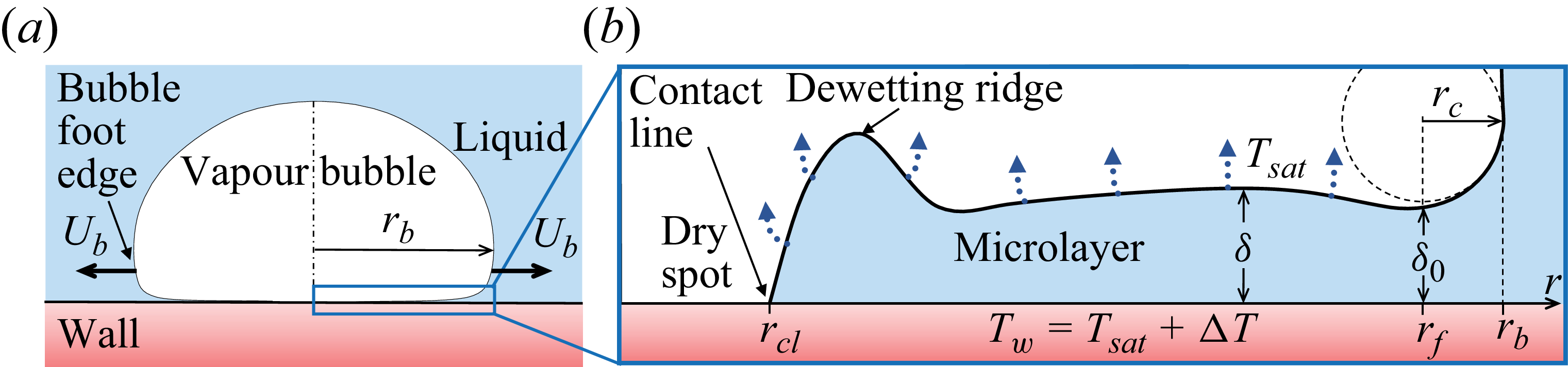
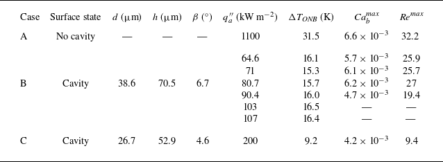


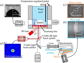


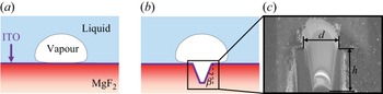



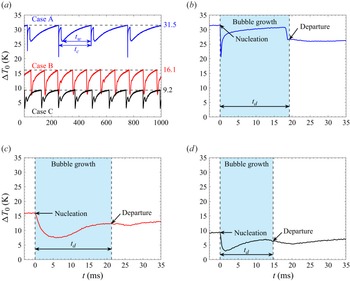


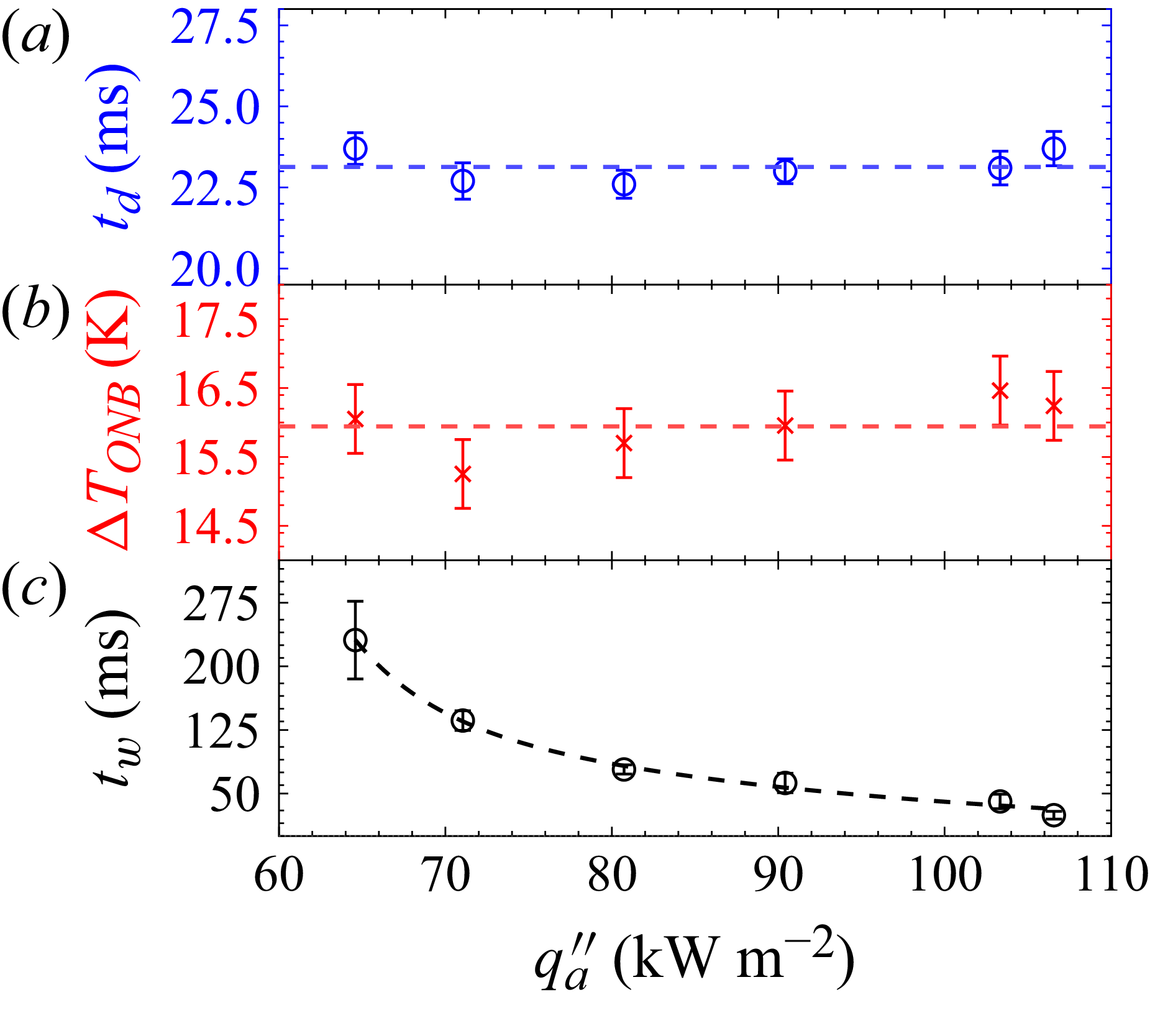


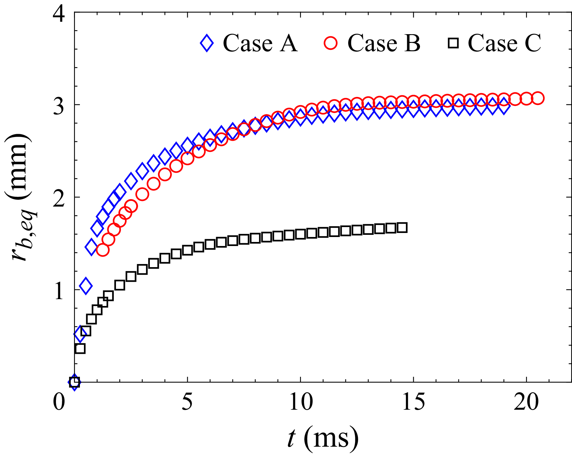


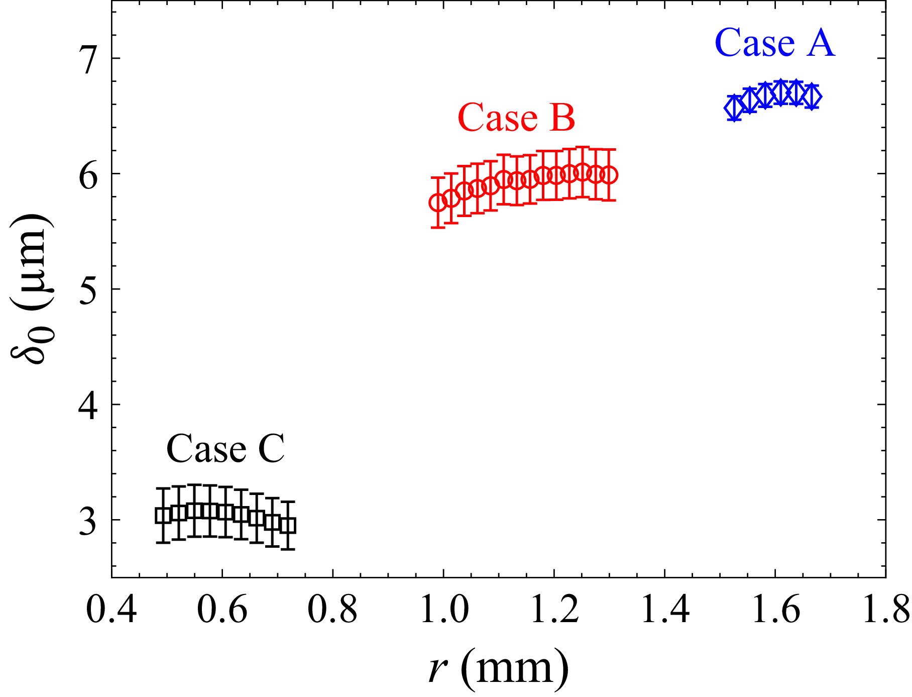


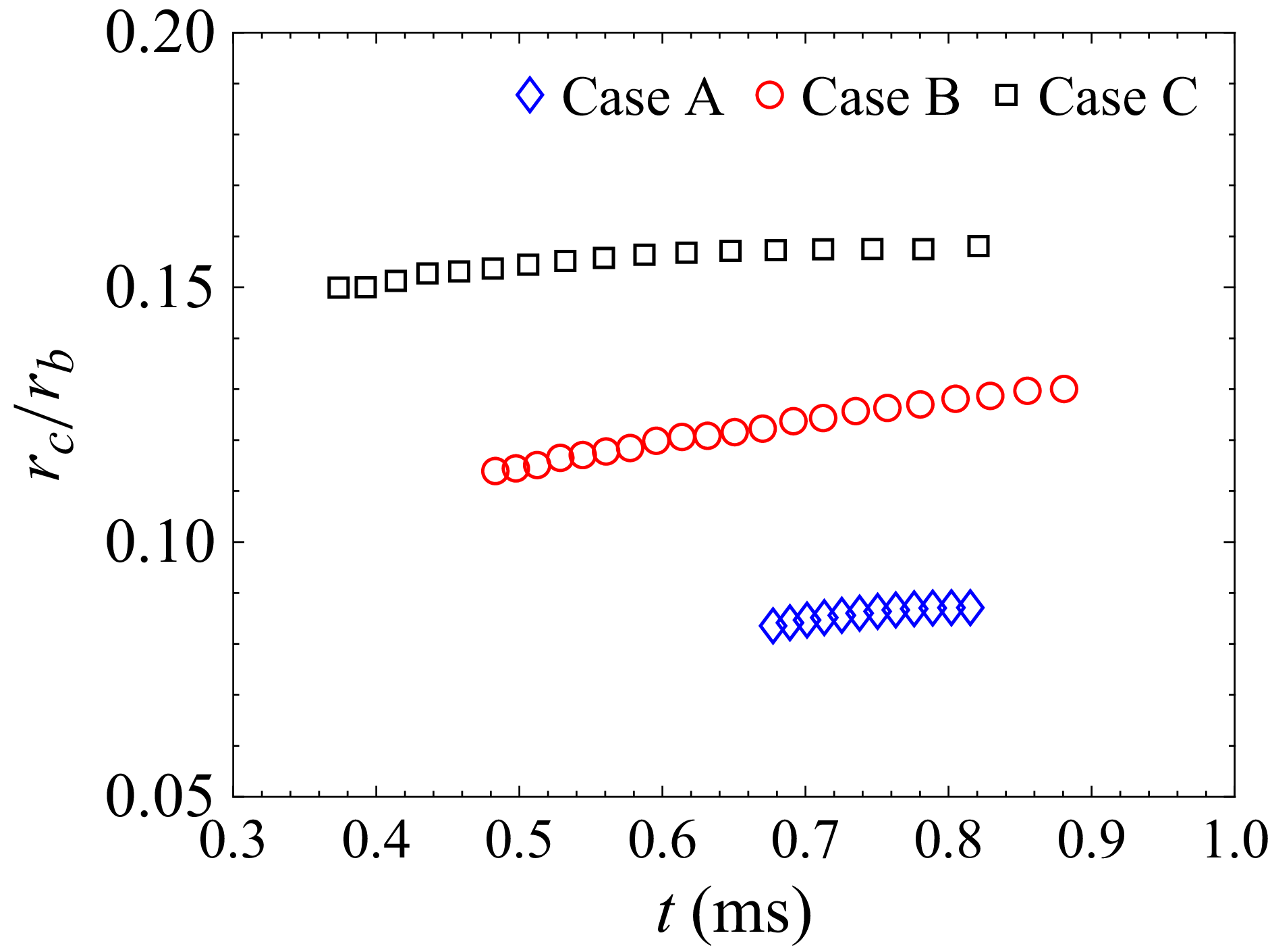


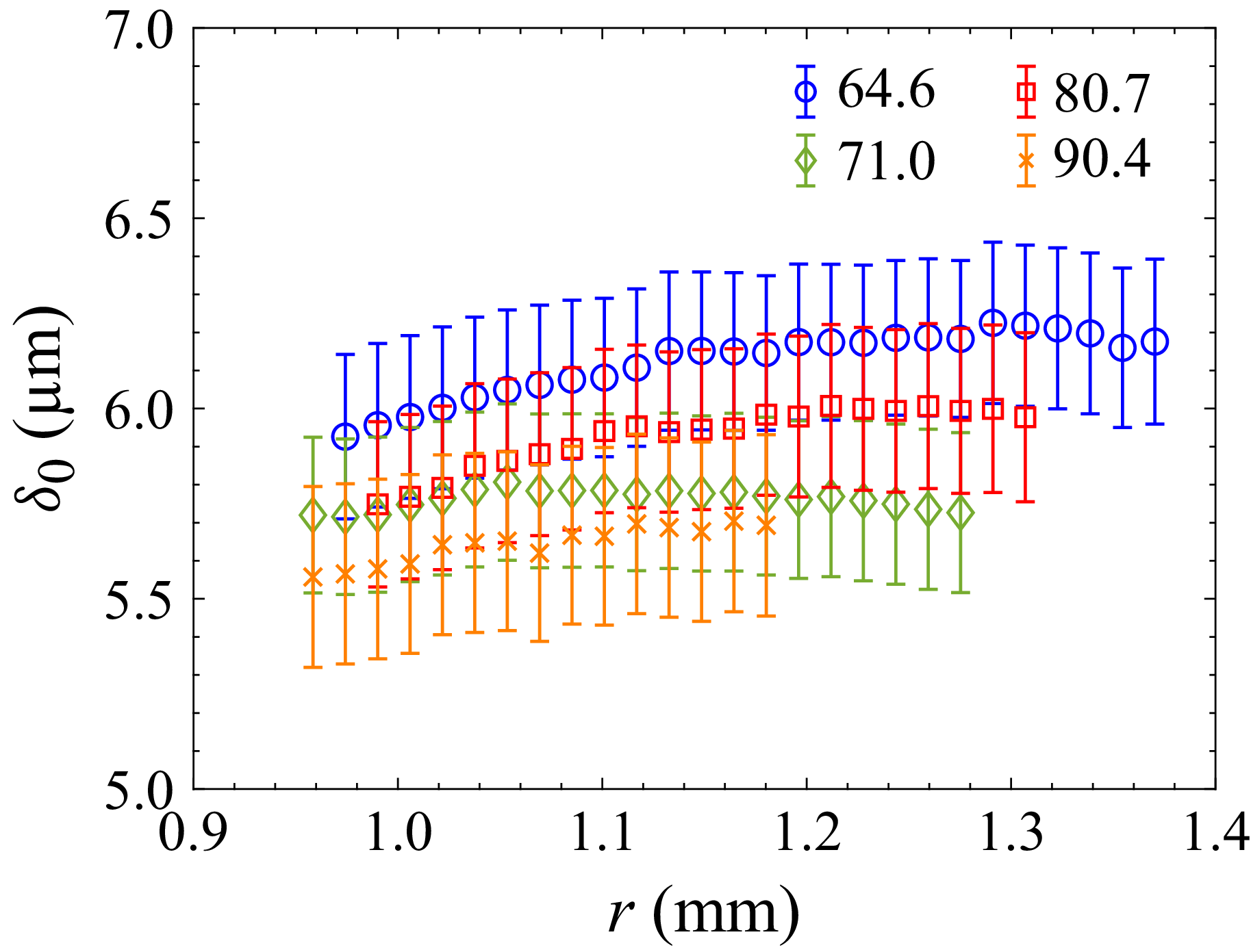


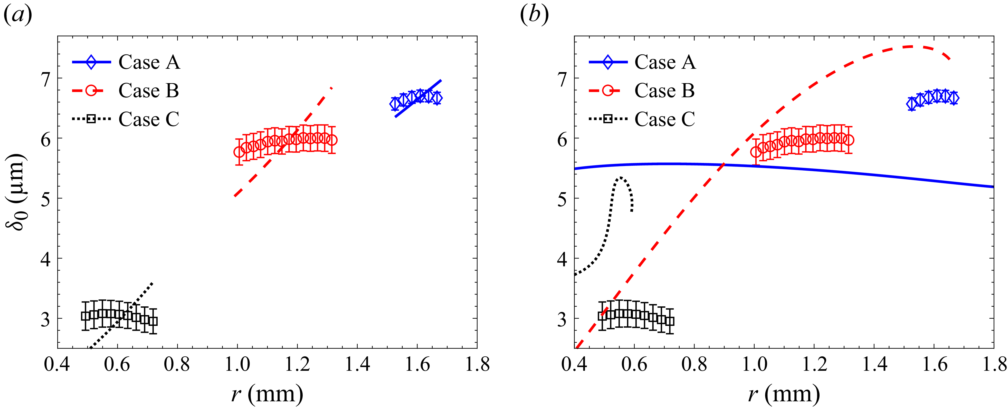
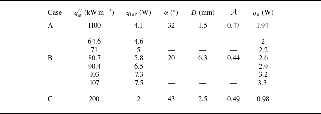


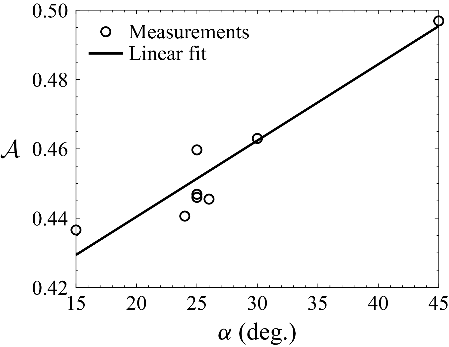


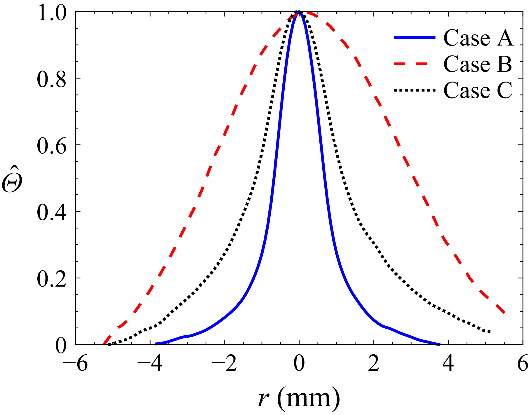


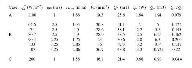





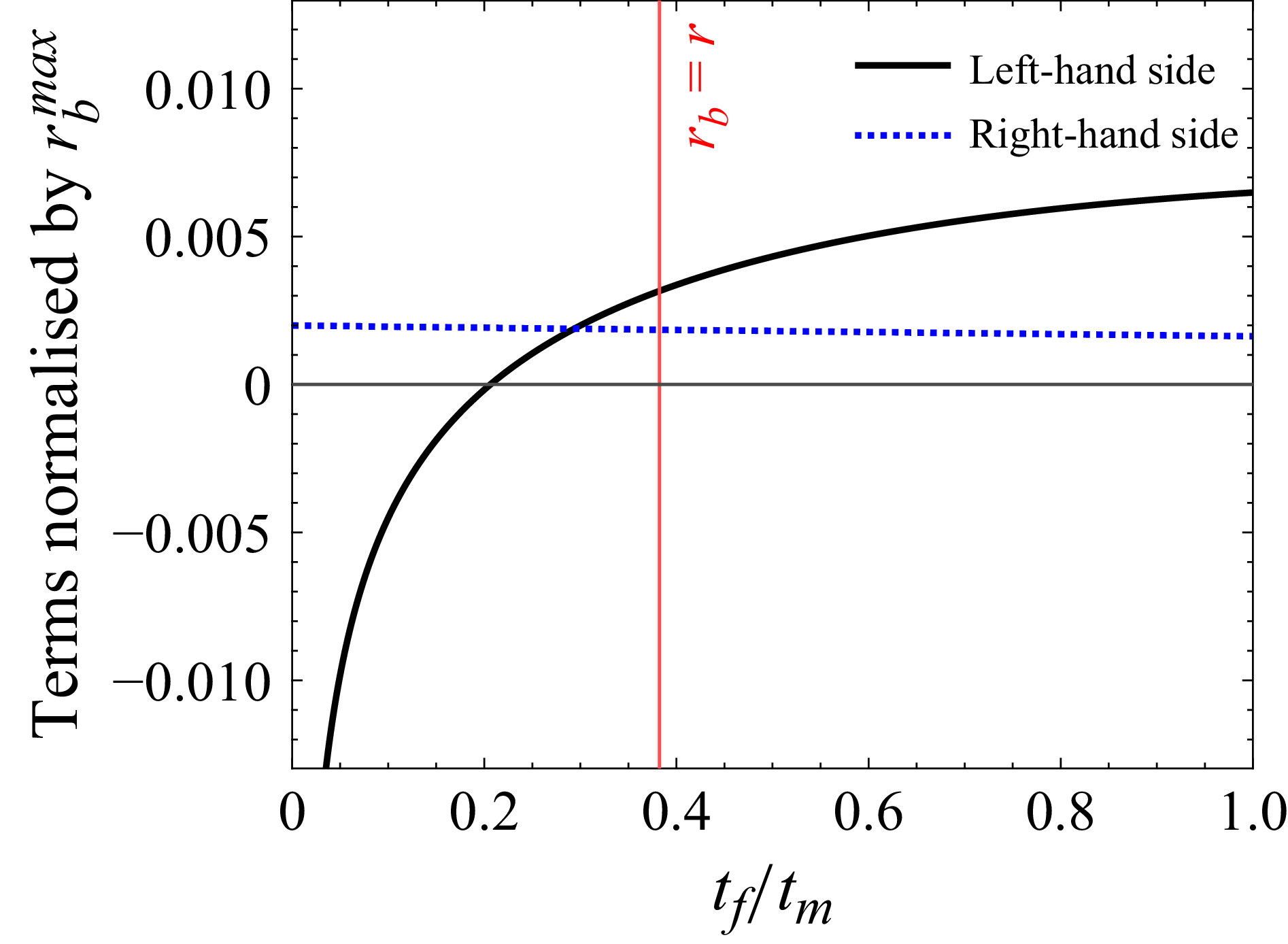


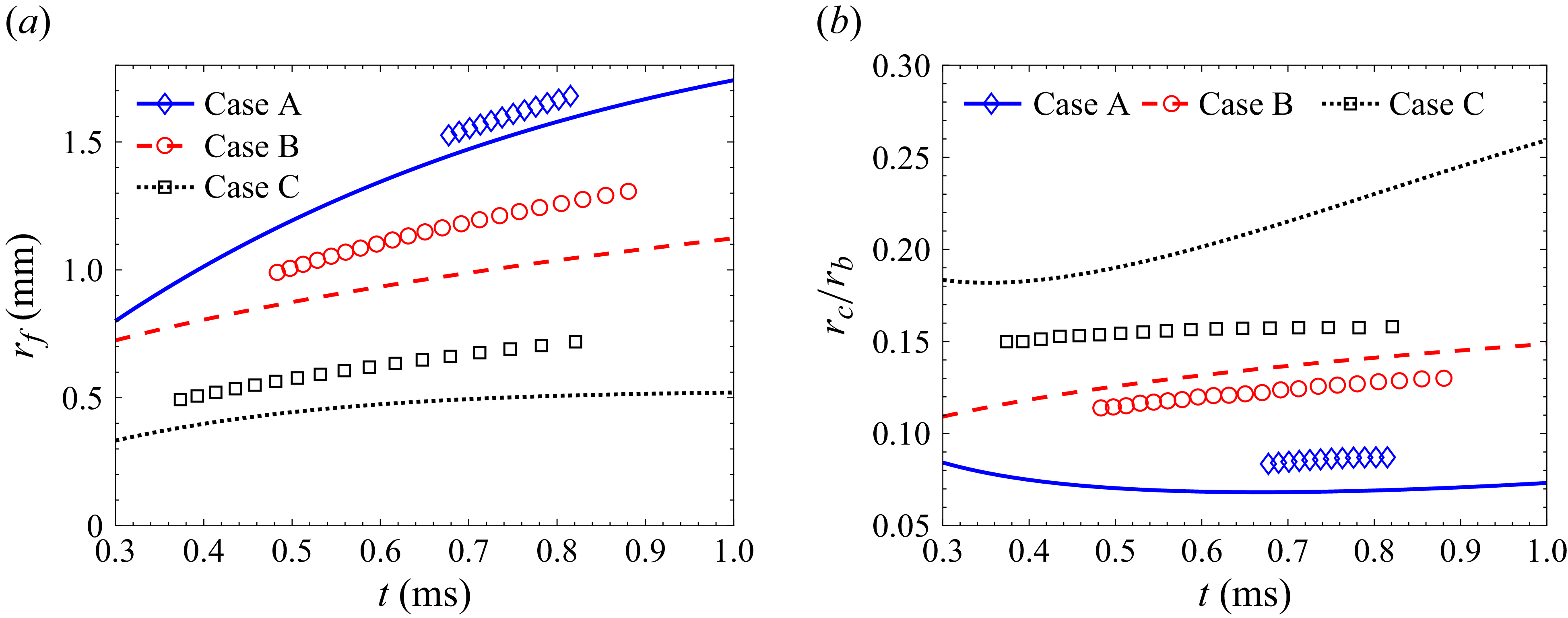


 Open access

