


INTRODUCTION
The Antarctic ice sheet is fringed by ice shelves and floating glacier tongues that account for 74% of its coastal margin (Bindschadler and others, Reference Bindschadler2011). Since the ice draining from the interior flows through these regions prior to entering the ocean (Rignot and others, Reference Rignot2008), understanding the dynamics of this floating ice is important (Pritchard and others, Reference Pritchard, Arthern, Vaughan and Edwards2009). Furthermore, a loss in the buttressing provided by ice shelves may lead to a catastrophic collapse of the Antarctic ice sheet (e.g., Fürst and others, Reference Fürst2016; Reese and others, Reference Reese, Gudmundsson, Levermann and Winkelmann2018). Studies on the dynamics of ice shelves and floating ice tongues are therefore crucial to elucidate how changes in stress balance propagate into the Antarctic interior. However, the rate of ice-shelf loss due to melting, thinning, hydrofracturing and eventual collapse remains poorly understood and requires in situ knowledge of the state of the ice itself.
Previous studies have shown that ocean tides have a strong influence on along-flow and vertical ice-shelf motion (King and others, Reference King, Makinson and Gudmundsson2011; Makinson and others, Reference Makinson, King, Nicholls and Hilmar Gudmundsson2012; Robel and others, Reference Robel, Tsai, Minchew and Simons2017). For example, King and others (Reference King, Makinson and Gudmundsson2011) reported that Larsen C Ice Shelf exhibits a ±10% variance in ice flow speed from its long-term mean value at fortnightly timescales, with up to ±100% variance at diurnal timescales. Furthermore, it is known that these tide-modulated ice-shelf flow variations also influence the basal shear stress at the ice/bed interface of the nearby grounded ice, with this effect propagating many tens of kilometres into the interior from the grounding line (Anandakrishnan and others, Reference Anandakrishnan, Voigt, Alley and King2003; Gudmundsson, Reference Gudmundsson2006). However, the amplitudes and phases of these variations are different among the Antarctic ice shelves (Makinson and others, Reference Makinson, King, Nicholls and Hilmar Gudmundsson2012; Robel and others, Reference Robel, Tsai, Minchew and Simons2017), indicating that complex mechanisms link tide-modulated ice-shelf processes. There is a limited number of in situ observations near the calving fronts of ice shelves and floating ice tongues in Antarctica.
There has recently been a substantial increase in glacier-seismicity studies that have recognized icequakes as a proxy of glacier dynamics and fracture mechanisms (e.g., Podolskiy and Walter, Reference Podolskiy and Walter2016; Aster and Winberry, Reference Aster and Winberry2017). For example, several studies have been conducted near the grounding lines of Antarctic ice shelves (Zoet and others, Reference Zoet, Anandakrishnan, Alley, Nyblade and Wiens2012; Barruol and others, Reference Barruol2013; Hammer and others, Reference Hammer, Ohrnberger and Schlindwein2015; Hulbe and others, Reference Hulbe2016; Lombardi and others, Reference Lombardi2016), as well as near an ice-shelf front (Pirli and others, Reference Pirli, Hainzl, Schweitzer, Köhler and Dahm2018), with tide-modulated seismicity observed in each instance. Hammer and others (Reference Hammer, Ohrnberger and Schlindwein2015) observed hybrid icequakes, which have high-frequency onsets (~8 Hz), followed by low-frequency coda (1–2 Hz), near the grounding line of Ekström Ice Shelf, East Antarctica. They observed that the maximum rate of icequakes occurred during mid-rising and high tides. Similarly, Lombardi and others (Reference Lombardi2016) observed low-frequency (1–10 Hz) icequakes during rising and high tides at an ice shelf in Dronning Maud Land, East Antarctica. These studies hypothesized that the observed icequakes were generated by basal processes, such as the opening of basal crevasses due to ice-shelf bending. A seismic array was also deployed near the ice-front of Fimbul Ice Shelf, East Antarctica, where Pirli and others (Reference Pirli, Hainzl, Schweitzer, Köhler and Dahm2018) suggested that a stick–slip motion generated low-frequency seismicity (2–6 Hz) during rising tides at the ice/rock interface, where the ice shelf was locally grounded. These examples suggest that the physical mechanisms generating tide-modulated icequakes vary greatly (for more examples, see Podolskiy and others Reference Podolskiy2016). However, studies near the calving fronts of floating glacier tongues are limited. Furthermore, the greatest difficulty in making definitive interpretations of tide-modulated seismic signals is the lack of concurrent high-resolution ice motion measurements, which are lacking in most of the above-mentioned studies. Such simultaneous seismic and geodetic observations are crucial in relating the seismic signals to glacial processes, such as the relationship between the longitudinal strain rate and co-seismic crevassing (Podolskiy and others, Reference Podolskiy2016).
We acquired geodetic and seismic measurements on the floating part of Langhovde Glacier, East Antarctica, over a 2-week period in January 2018, to study ice-shelf dynamics. While the glacier is relatively small for Antarctica, it has a typical floating ice tongue that is observed at the front of numerous glaciers throughout Antarctica. The relatively small floating tongue enabled us to deploy a linear array of global navigation satellite system (GNSS) stations along the floating ice tongue, stretching from the ice front to the grounding line. A passive seismic array was also installed 500 m from the ice front. Here we present an analysis of temporal variations in the detected icequake activity and their relationship to the observed ice-motion and ocean-tide records. This dataset enables us to investigate tide-modulated ice dynamics and possible mechanisms for generating icequakes near the terminus of this East Antarctic floating glacier.
STUDY SITE
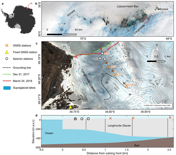
Langhovde Glacier (69°11'S, 39°32'E) is located on the Soya Coast, East Antarctica and drains into Lützow–Holm Bay ~20 km to the south of the Japanese Syowa Station (Fig. 1). Langhovde Glacier is 3 km wide and flows at a rate of 130 m a−1 near the ice front (Sugiyama and others, Reference Sugiyama, Sawagaki, Fukuda and Aoki2014). The fast-flowing part is ~10 km long. The lower 2–3 km of the ice surface is flat, suggesting the formation of a floating shelf (Fig. 1c) (Fukuda, Reference Fukuda2014). Recent hot-water drilling has confirmed that this region is floating and ice is 234–412 m thick (Fig. 1d) (Sugiyama and others, Reference Sugiyama, Minowa, Ito and Yamane2018). Satellite data analysis between 2000 and 2012 shows that recent fluctuations in the glacier terminus have probably been controlled by concentration of thick land-fast ice in the bay which affected calving (Fukuda and others, Reference Fukuda, Sugiyama, Sawagaki and Nakamura2014). The ice front advanced by 380 m after 2007 until 2011 which followed by 200 m retreat due to calving. Tide-modulated vertical ice motion has previously been observed on Langhovde Glacier using GNSS stations, with ~1.5 m of vertical ice motion observed near the ice front that progressively decreases toward the grounding line (Sugiyama and others, Reference Sugiyama, Sawagaki, Fukuda and Aoki2014).
(a) Location of the study region with respect to Antarctica. (b) Landsat 8 satellite image of the study region acquired on 5 November 2017. The red rectangle highlights the location of Langhovde Glacier. (c) Closeup image of Langhovde Glacier and instrument locations. The background image was acquired by Plèiades on 21 December 2017. The black curves denote the ice surface contours at 10-m intervals. The estimated grounding line by the break in slope method is highlighted by the black dashed curve (Fukuda, Reference Fukuda2014). (d) Along-flow cross-sectional profile of Langhovde Glacier. The ice geometry and seafloor bathymetry were directly measured via four boreholes during the 2018 field campaign, which are indicated by vertical gray lines (Sugiyama and others, Reference Sugiyama, Minowa, Ito and Yamane2018). The ice shelf bottom geometry was obtained by piecewise cubic interpolation using the borehole data.
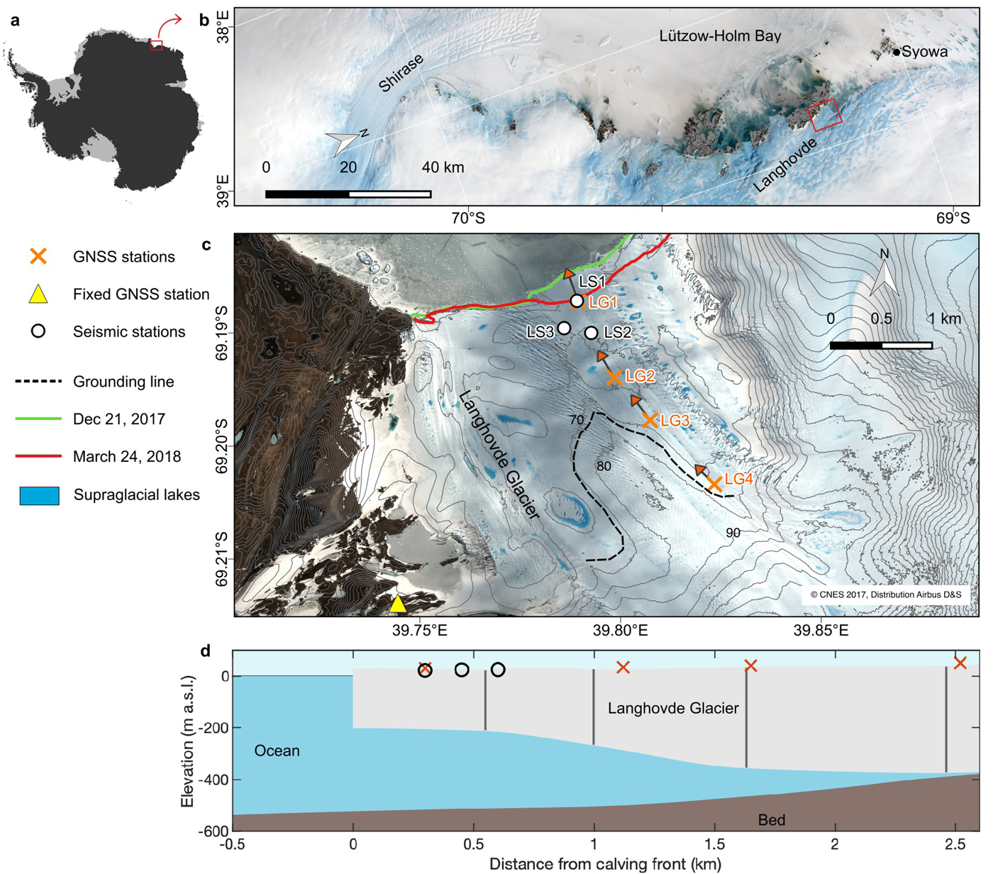
The daytime air temperature often exceeds 0°C across Langhovde Glacier from late December until late February (Langley and others, Reference Langley, Leeson, Stokes and Jamieson2016), causing ice melting and leading to the formation of supraglacial lakes and streams, as observed during the present study period (Fig. 1c). It should be noted that bare ice is exposed on the glacier surface for most time of the year because strong katabatic wind prevents snow deposition.
METHODS
Along-flow and vertical ice motion
We installed four dual-frequency GNSS receivers at LG1–4 (GNSS Technologies, GEM-1) on the ~3-km-long floating ice tongue, positioned 0.3–2.5 km from the ice front, that operated between 31 December 2017 and 23 January 2018 (Fig. 1c). The GNSS antennae were mounted on top of 2-m-long aluminum poles drilled into the ice. We calculated the three-dimensional coordinates of the GNSS antennae every 15 min using data from a fixed GNSS station that was located on the western side of Langhovde Glacier (Fig. 1c). We processed the data using the RTKLIB software package with static method. The horizontal and vertical accuracies are expected to be 2–3 mm and 3–5 mm, respectively, for our ~3 km baseline length (Sugiyama and others, Reference Sugiyama, Sawagaki, Fukuda and Aoki2014).
Icequake detection and monitoring
The seismic array consisted of three seismometers installed at LS1–3, 0.5 km from the ice front and with an array aperture of ~300 m, that operated between 8 and 24 January 2018 (Fig. 1c). Lennartz LE-3Dlite MkIII/1s seismometers with a flat response approximately between 1 and 200 Hz, were connected to Omnirecs DATA-CUBE3 recorders and powered by solar panels and external batteries. Each sensor was installed in a 0.2 m-deep ice pit and covered by a metal net and white cloth to reduce ice melting and noise due to the wind. The sample rate was 400 Hz for each station, higher than that in previous similar studies (Barruol and others, Reference Barruol2013; Hammer and others, Reference Hammer, Ohrnberger and Schlindwein2015; Hulbe and others, Reference Hulbe2016; Lombardi and others, Reference Lombardi2016; Pirli and others, Reference Pirli, Hainzl, Schweitzer, Köhler and Dahm2018). We visited the stations 2 or 3 times for level/orientation checks and data backup, which had negligible impact on results presented below. We recognized that such visits were necessary due to intense surface melting and water ponding. Unlike glaciers with a considerable slope gradient, where the pit containing the surface sensor can be provided with a drain channel (e.g., Podolskiy and Walter, Reference Podolskiy and Walter2016), the flat surface of the glacier inhibits effective drainage (Fig. 1c). This flat surface topography, together with surface melt makes future seismic observations technologically challenging.
Here we focus on the vertical component of station LS1, since it represents well the overall temporal variation in seismicity, which was similar between all seismic stations due to their close proximity. We note that this similarity holds despite the fact that LS1 was positioned near a rift on the glacier, which led to a major calving event that occurred 2 months after the campaign (Fig. 1c).
The icequakes were detected using the classic STA/LTA (short-term averaging/long-term averaging) method implemented in ObsPy, a Python toolbox for seismology (Beyreuther and others, Reference Beyreuther2010). Here we used 0.2 and 5.0 s window lengths for the STA and LTA, respectively, which were similar to those used in previous studies (Barruol and others, Reference Barruol2013; Podolskiy and others, Reference Podolskiy2016). We applied bandpass-filter between 1 and 180 Hz before detection. Since two distinct signal types were observed at different frequency bands (1–30 Hz and 30–180 Hz, described later), we applied the method to each band separately. We acknowledge that more advanced detection methods (e.g., Podolskiy and Walter, Reference Podolskiy and Walter2016) might yield further insights in follow-up studies of this dataset.
Seismic signal processing
We performed spectral analysis of the observed signals to investigate their seismic wave properties. We first calculated spectrograms of the identified seismic events by using the MATLAB ‘spectrogram’ function, with a 20–40-sample window and 90% overlap (these parameters were chosen empirically to optimize the temporal and frequency resolution). We also calculated the power spectral density (PSD) using the MATLAB ‘fft’ function and 28 sample points.
The continuous seismic signals were processed in two ways. We first calculated the temporal evolution of the PSDs for 1 min segments of the seismic signals to generate a long-term spectrogram. These PSDs were also used to observe any statistical differences in the seismic signals due to the tidal phases: rising, falling, high and low tides. We defined the high- and low-tide seismicity to be within an hour of the semi-diurnal maxima and minima, respectively, with the rising- and falling-tide seismicity classified as occurring during either the rising or falling tide. We then applied such classification to the 2-week-long seismic records. Finally, the probability density functions (PDFs) of the PSDs were generated using the method introduced by McNamara and Buland (Reference McNamara and Buland2004). Following this method, the seismic traces were deconvolved from the instrument response, parsed into 60-second segments, and analyzed using a 50% overlap between neighboring segments. The obtained PSDs were smoothed in full-octave averages at 1/8-octave intervals. Further technical details on PSD-PDFs can be found in McNamara and Buland (Reference McNamara and Buland2004).
Tidal observations
The tidal record at Syowa Station (Fig. 1b), which is located ~20 km north of the glacier, was decomposed to investigate the tidal components (Aoyama and others, Reference Aoyama2016). These components were used to predict the tidal phases between 9 and 23 January 2018 at the glacier using BAYTAP-G software package (Tamura and others, Reference Tamura, Sato, Ooe and Ishiguro1991).
RESULTS
Ice motion
Diurnal and semi-diurnal variations in ice motion were observed at each of the GNSS stations over the 2-week observation period (Fig. 2). These variations were closely related to the tidal variations except at LG4, which was located near the grounding line (Fig. 1c). The along-flow displacements where in anti-phase with the tides, with the maximum (minimum) along-flow displacement rate observed during falling (rising) tide at LG1–3 (Fig. 2b). The diurnal variation at LG1 exhibits a maximum deviation from mean displacement up to 0.08 m during 14–20 January. The mean along-flow velocity was 0.35, 0.31, 0.30 and 0.27 m d−1 for LG1, 2, 3 and 4, respectively.
(a) Trajectories of the four GNSS stations since 9 January. Time-evolution of (b) along-flow and (c) vertical ice motion observed at GNSS stations LG1–4. The gray curves indicate the modeled tidal variations and vertical dash-dotted gray lines indicate low tide. (d)–(g) Map view of tide-induced glacier displacement, after removal of the mean displacement. The dots are colored according to the January 2018 hourly observations. Orientation of the displacement determined by a linear regression (clockwise from north) is indicated in the upper left corner of each panel. Black arrow and the number below are mean along-flow glacier speed and direction.
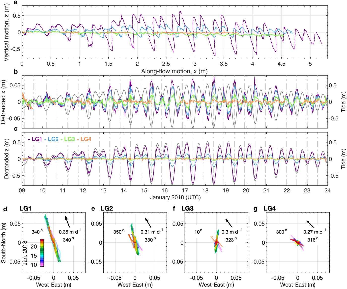
Similar tide-modulated diurnal and semi-diurnal fluctuations were observed for the vertical motion, but they were an order of magnitude larger than the along-flow motion (Fig. 2c). The phase and amplitude of the vertical motion were remarkably similar to those of the tidal variation (Fig. 2c), with the higher peaks occurring at high tide, and vice versa.
Regular back-and-forth along-flow motion was observed at LG1, LG2, LG3 and LG4 after removing the mean displacement, where the ice moved along the 340°, 350°, 10° and 300° directions, respectively (Figs 2d–g). In general, these directions of motion aligned with the principal direction of the ice flow with the exception of the station LG3, which had declined from the rest of the stations during high-amplitude tide probably due to the influence of nearby grounded ice (Fig. 2f). The glacier movement decelerated and accelerated during the rising and falling tides, respectively (Fig. 2a).
Types of icequake
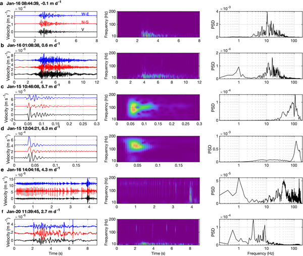
We identified several types of icequake via visual inspection of the vertical and horizontal components of the seismic traces recorded at LS1 (Fig. 3). The discussed types could be seen across the entire seismic array. We observed two principal families of events with similar dominant frequencies: a low-frequency (~10 Hz) group (Figs 3a and b) and a high-frequency (~120 Hz) group (Figs 3c–e).
Waveforms, spectrograms and power spectral density (PSD) plots of the visually identified events at LS1. The blue, red and black curves show the west-east, north-south and vertical components of the waveforms, respectively. (a)–(b) Typical low-frequency events. (c)–(d) Typical high-frequency events. (e) Repeating events. (f) Mixed event. The observed time of each event and its corresponding vertical tidal velocity are indicated above the waveforms.

The waveforms of the low-frequency group had no distinct P and S arrivals and no significant differences among the seismic components. This group has an emergent onset and long-lasting coda train (5–10 s) (Figs 3a and b). Two types of event were recognized: one with a dominant frequency of ~10 Hz and a relatively impulsive onset and decay (Fig. 3a); and one that resembled a tremor, with a slightly higher dominant frequency (13 Hz) and more emergent onset (Fig. 3b).
The high-frequency group is characterized by an impulsive, broadband onset and a frequency bounded by the Nyquist frequency of the dataset (200 Hz). This group consists of short-duration events with a clear onset that decayed in 1 second or less, and a dominant frequency of ~100 Hz (Figs 3c–e). Three types of event were observed within this group: i) one with a 100 Hz characteristic frequency (Fig. 3c), ii) one with an impulsive onset followed by high-frequency monochromatic ringing at 160 Hz (Fig. 3d), and iii) one with repeating high-frequency icequakes (120 Hz), whose inter-event interval gradually decreased from ~14 to 7 events per second (Fig. 3e) (we note that these small repeaters were not detected with our STA/LTA algorithm). The energy of this drum-like signal was predominantly observed in the horizontal components.
A hybrid, or a mixture, of these high-/low-frequency events was also observed (Fig. 3f). These events had low-frequency onsets (10 Hz), followed by lower-frequency coda (3 Hz) overlapping high-frequency (~130 Hz) events (Fig. 3f).
Temporal variations of icequakes
The observed icequake activity exhibits a highly non-uniform distribution over the 2-week study period (Fig. 4). The RMS amplitudes of the seismic signals, shown in Fig. 4a, indicate that the highest peak amplitudes occur during rising and high tides. These high RMS amplitudes correspond to high spectral power over the entire frequency band, between 1 and 180 Hz (Fig. 4b). A power drop above 180 Hz to Nyquist frequency results from a limitation in instrument response. A small increase in power was observed at ~10 Hz during the falling tide (Fig. 4b). A notable increase in seismic noise was sometimes present in the 100–150 Hz frequency range during 10–16 January, but without a clear relationship to the tidal phase (Fig. 4b).
(a) RMS seismic amplitude and vertical ice-motion anomaly at LG1. (b) Time-evolution of the PSDs computed for 1-min segments of the seismic signals. The color scale is in dB (proportional to 20log10(counts2 Hz−1)). The number of (c) unfiltered and (d) bandpass-filtered (1–30 Hz (blue) and 30–180 Hz (red)) hourly icequakes at LS1. The vertical dotted gray lines show the timing of the rising tides. The vertical ice-motion anomaly at LG1 is also provided in (c). (e) Hourly wind speed (green) and air temperature (red) records observed at Syowa Station.
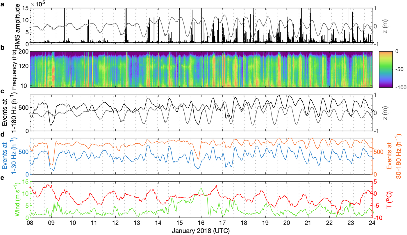
We detected 218,477 icequakes during the 2-week study period at LS1 using the detection parameters described in the Methods section, with a mean occurrence rate of ~ 500 events h−1 (Fig. 4c). The icequake occurrence rates exhibited diurnal and semi-diurnal variations that changed over time (Fig. 4c). Only the diurnal peak was significant during 8–14 January, although a semi-diurnal peak, with an amplitude that was much smaller than the diurnal variation, was also present. This semi-diurnal signal became clearly noticeable after 14 January (Fig. 4c).
We ran our STA/LTA icequake detector for two separate frequency bands, 1–30 Hz and 30–180 Hz, since we categorized all the observed icequakes into two families. These searches yielded 168,464 and 284,902 icequakes, respectively (Fig. 4). The average hourly occurrence rates were 400 and 670 events h−1 for the 1–30 Hz and 30–180 Hz frequency bands, respectively. Such high rate of background seismicity is expected because the floating tongue and the grounded part of the glacier are in a state of continuous motion, which leads to greater strains at the free surfaces and shear margins. The diurnal and semi-diurnal variations were more prominent in the low-frequency band, especially before the 15 January, when there was no clear diurnal variations in the high-frequency band.
Time series of air temperature and wind speed measured at Syowa Station (Fig. 4e) suggest that there is no obvious relationship with the seismic activity. For example, the air temperature showed no semi-diurnal variations. Wind speed was relatively low (median value was 4.3 m s−1), and no anomaly in the spectrogram was observed on the day with strong winds (15 January 2018) (Fig. 4b). Nevertheless, it is possible that reduced number of detection on 8--9 January, could be due to elevated noise levels from intense melt following warm temperatures of 8 January.
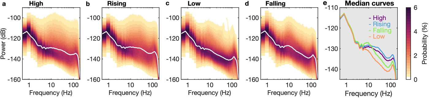
Figure 5 illustrates the PSD-PDFs dependence on the tidal phases. The power distribution generally exhibited a degree of similarity among all of the tidal phases, especially below 5 Hz. Elevated power levels were observed at ~10 Hz and above 100 Hz (Fig. 5). Differences could be seen between the high/rising (Figs 5a and b) and low/falling tides (Figs 5c and d), with the PSD-PDFs for the high/rising tides possessing higher power levels over a wide frequency band above 10 Hz (for ~5 dB). This is consistent with the elevated levels of seismicity during rising and high tides, which we earlier quantified using the RMS and STA/LTA approaches. We also note that the PSD-PDFs for the falling tide (Fig. 5d) had slightly higher power at ~10 Hz, which we will revisit in the Discussion section.
PSD-PDFs representing the different tidal phases for the 2-week observation period at LS1. The power is relative to m2 s−2 Hz−1. The white curve shows the median power for each PDF distribution.
Icequake duration and magnitude
The duration of the icequakes detected in the 1–180 Hz frequency band was below 2 s for ~95% of the events, with a median duration of 0.42 s (Fig. 6a). The durations estimated using two different bandpass filters (1–30 Hz and 30–180 Hz) yielded different results (Fig. 6a). The median duration in the 1–30 Hz band (0.66 s) was approximately twice that in the 30–180 Hz band (0.33 s), as shown in Fig. 6a.
(a) Empirical cumulative distribution functions (CDFs) of icequake duration (0.1 s bins) and (b) duration magnitude, M d, for ~220,000 events detected at LS1 during the 2-week observation period. The open circles are the median icequake duration and duration magnitude. The numbers are given (in parentheses) in the respective legends.
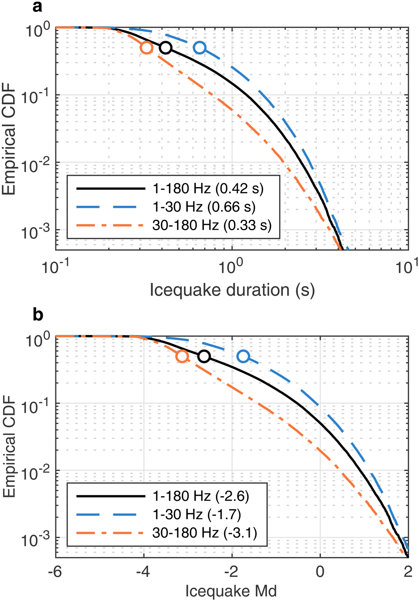
The majority of these durations correspond to negative M d values, defined as M d ~ −0.9 + 2log(d) (Lee and others, Reference Lee, Bennett and Meagher1972; Barruol and others, Reference Barruol2013). The range of estimated M d values was between −4 and −1, with M d ≈ −3 most likely representing the magnitude of completeness for the dataset (Fig. 6b). The median icequake M d was between −3.1 and −1.7, depending on the frequency band considered (Fig. 6b).
DISCUSSION
Tide-modulated ice motion
Elastic behavior of the floating tongue
The observed along-flow and vertical ice motions are closely related to the tidal fluctuations (Fig. 2). There is an anti-phase relationship between the along-flow ice motion and tidal oscillations (Fig. 2b). This corresponds to the maximum (minimum) ice speed during the falling (rising) tide. It is known that an elastic material reacts to stress via an instantaneous displacement (Christmann and others, Reference Christmann, Plate, Müller and Humbert2016a, Reference Christmann, Rückamp, Müller and Humbertb). The displacement for a purely elastic response would be therefore in anti-phase to the tidal forcing. This agrees with our observations at Langhovde Glacier (Fig. 2), where the ocean-tide-induced hydrostatic pressure acts on the glacier. A similar elastic behavior explains the flexure of Antarctic ice shelves well (Vaughan, Reference Vaughan1995), and also the timing of the basal seismicity of Kamb Ice Stream (Anandakrishnan and Alley, Reference Anandakrishnan and Alley1997). In contrast to our findings, several other possible mechanisms have been reported in the literature to explain the along-flow motion of ice shelves (e.g., Doake and others, Reference Doake2002; Legrésy and others, Reference Legrésy, Wendt, Tabacco, Rémy and Dietrich2004; Brunt and others, Reference Brunt, King, Fricker and MacAyeal2010; King and others, Reference King, Makinson and Gudmundsson2011; Makinson and others, Reference Makinson, King, Nicholls and Hilmar Gudmundsson2012; Robel and others, Reference Robel, Tsai, Minchew and Simons2017), as follows.
1. Changes in ice/water friction due to tidal currents: One of the first GPS measurements on Brunt Ice Shelf suggested that the maximum ice flow speed occurred ~4 hours before high tide, which might be related to the sub-shelf ocean current (Doake and others, Reference Doake2002). Similar mechanisms were inferred to explain the dynamics of Mertz Ice Tongue (Legrésy and others, Reference Legrésy, Wendt, Tabacco, Rémy and Dietrich2004).
2. Changes in basal drag: reduction in basal drag during high tides might enhance ice motion (Minchew and others, Reference Minchew, Simons, Riel and Milillo2017; Robel and others, Reference Robel, Tsai, Minchew and Simons2017).
3. Tilting of the ocean surface: King and others (Reference King, Makinson and Gudmundsson2011) reported that tilting of the sea surface at Larsen C Ice Shelf modulated its ice motion. The maximum (minimum) ice flow speed of the ice shelf was observed during the rising (falling) tide.
It appears that these above-mentioned mechanisms are not adequate to explain the diurnal and semi-diurnal along-flow variations of Langhovde Glacier, where the maximum ice flow speed is observed during the falling tide (Fig. 2). This might reflect the smaller ocean-tide amplitudes in Lützow–Holm Bay compared with other Antarctic regions (Padman and others, Reference Padman, Siegfried and Fricker2018) and the very low tidal current (20–30 mm s−1) observed via borehole measurement near the grounding line of Langhovde glacier (Sugiyama and others, Reference Sugiyama, Sawagaki, Fukuda and Aoki2014), which indicate that hydrostatic stress acting on the glacier front is a dominant process compared with other mechanisms when tidal forcing is limited.
Spatial response of ice motion to ocean tides
We calculated the daily value of the tidal admittance, Λ, which is defined as the ratio between the tidal response and the tidal height, H (de Juan and others, Reference de Juan2010; Podrasky and others, Reference Podrasky, Truffer, Lüthi and Fahnestock2014), to further investigate the tidal influence on floating tongue motion, such that:
 $$ \chi^2_{m,\;n} = {{[\xi_{\rm lin}-\Lambda_{{\rm m}}{H} (t-\delta t_n)]^2} \over {\sigma_{\xi}^2}}, $$
where we searched a matrix (m, n) of Λm values and time delays, δt n, to find the best-fitting model for the tidal response that minimizes the χ 2 difference between the detrended position, ξ lin, and modeled position, ΛmH(t − δt n), while accounting for the position uncertainty, σ ξ. The tidal admittance represents how the ocean-tide influence propagates up-glacier as a function of time and distance.
Furthermore, we apply a simple analytical model for tidal admittance, Λ, to explain the obtained spatial variation in the tidal response (Figs 7a and b). The previous observational studies suggested that the influence from tides on the ice motion decays exponentially with distance from the calving front (Anandakrishnan and Alley, Reference Anandakrishnan and Alley1997; de Juan and others, Reference de Juan2010; Podrasky and others, Reference Podrasky, Truffer, Lüthi and Fahnestock2014):
 $$ \Lambda(D)=\Lambda_0 {\rm e}^{-\beta D} $$
where D is the distance from the terminus, Λ0 is the initial Λ value and β is the decay constant.
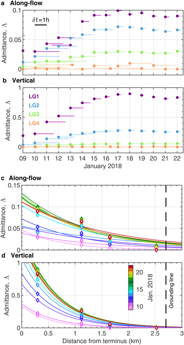
(a) along-flow and (b) vertical daily tidal admittance for the GNSS measurements. The horizontal bars indicate the time lag (δt) between the ocean tides and glacier displacements, where a right directed lag indicates that the tidal variation is ahead of glacier displacements. Daily (c) along-flow and (d) vertical tidal admittance, plotted as a function of distance from the calving front, together with the analytical best-fit curves. The data points are colored according to the January 2018 daily averages. The mean decay rate,  $\bar {\beta }$, is 0.8 and 1.6 km−1 for the along-flow and vertical tidal admittance, respectively. The vertical dashed black line indicates the estimated position of the grounding line.
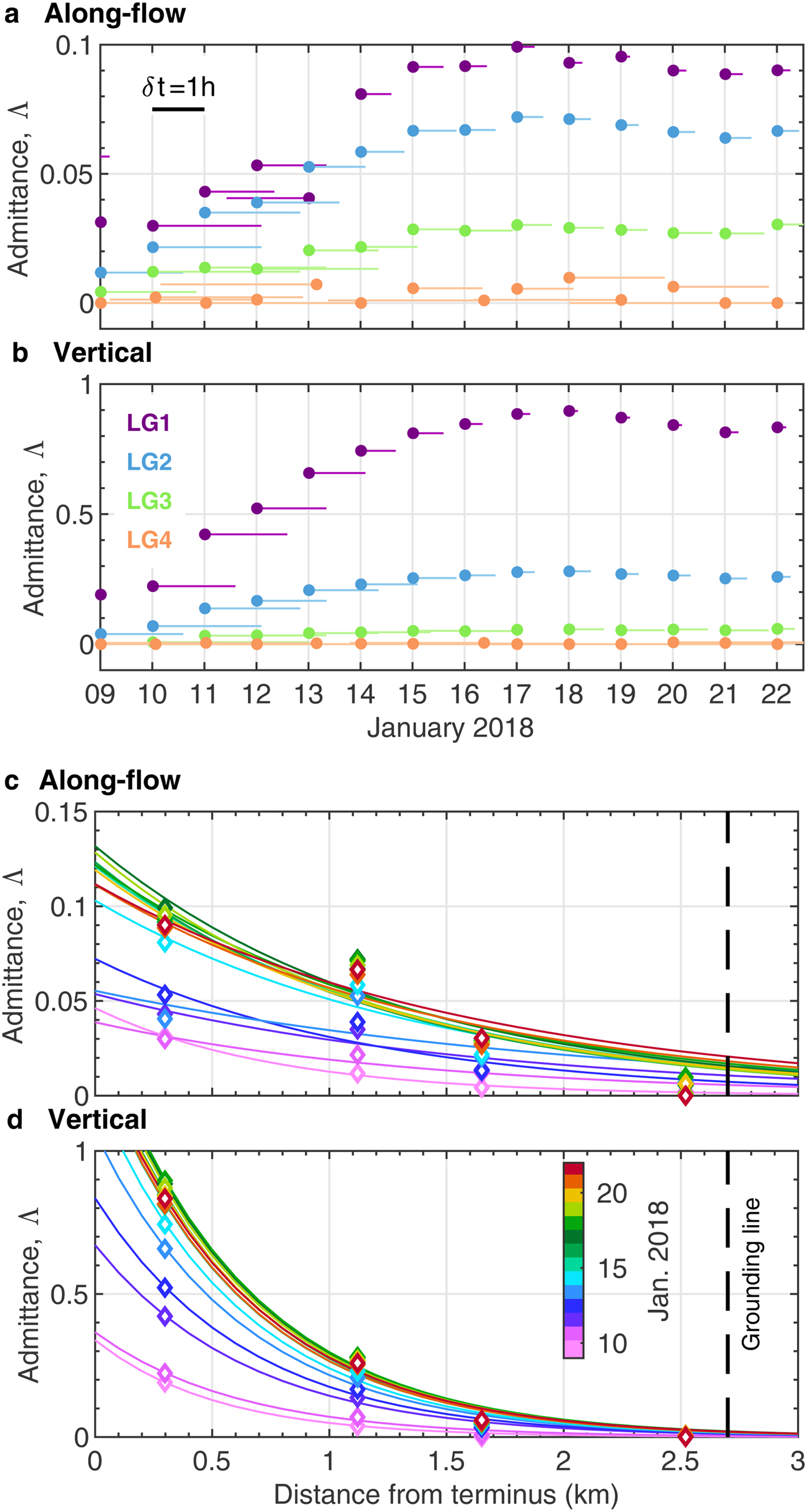
Both the along-flow and vertical tidal admittances increased over time during 9–13 January (Figs 7a and b), where the vertical and along-flow ice motions lagged the ocean tide by ~2 h in the first several days. This lag decreased as the admittance increased. The admittance maintained a high value from 15 January until the end of our experiment (Fig. 7). Figures 7c and d show the spatial admittance calculated via Equation 2. The decay constant, β, was twice as large for the vertical tidal admittance (1.6 km−1) as for the along-flow tidal admittance (0.8 km−1). The admittance decreased substantially from LG1 to LG2 (Fig. 7d). The tidal influence on the along-flow response propagates further up-glacier than the vertical response (Figs 7c and d).
The observed ocean-tide influence near the grounding line of Langhovde Glacier was much smaller than that observed in previous studies. The tidal influence on glacier motion has been extensively studied for West Antarctic ice streams (Harrison and others, Reference Harrison, Echelmeyer and Engelhardt1993; Anandakrishnan and Alley, Reference Anandakrishnan and Alley1997; Anandakrishnan and others, Reference Anandakrishnan, Voigt, Alley and King2003; Gudmundsson, Reference Gudmundsson2006; Aðalgeirsdóttir and others, Reference Aðalgeirsdóttir2008), with a tidal influence on ice motion observed up to 300 km from the grounding line of Whillans Ice Stream (Harrison and others, Reference Harrison, Echelmeyer and Engelhardt1993). Such significant propagation of the tidal signal is possible because basal sliding over a dilatant till layer contributes to most of the observed ice-stream motion, as opposed to internal deformation. These ice streams also have extensive flat areas, which indicate a limited degree of basal and lateral drag along the glacier boundaries. Therefore, a small perturbation to the stress balance due to ocean tides can effectively travel over large distances. Unlike the large and flat ice streams of West Antarctica, Langhovde Glacier has a relatively steep, narrow and bumpy ice surface upstream of the grounding line and is bound by slowly moving grounded ice (Fig. 1), indicating significant basal and lateral drags. This observation suggests that the interior of Langhovde Glacier is insensitive to external forcings such as ocean tides.
Seismicity due to tide-modulated ice motion
Basal/englacial origin seismicity (major peaks)
The most distinct icequake pulsations occurred during the mid-rising to high tides (Fig. 4), with RMS amplitude increasing substantially during these periods (Fig. 4a). Previous studies have reported greater seismicity during similar tidal phases, with low-frequency seismic signals below 10 Hz (Hammer and others, Reference Hammer, Ohrnberger and Schlindwein2015; Lombardi and others, Reference Lombardi2016; Pirli and others, Reference Pirli, Hainzl, Schweitzer, Köhler and Dahm2018). However, two different mechanisms have been proposed. Hammer and others (Reference Hammer, Ohrnberger and Schlindwein2015) and Lombardi and others (Reference Lombardi2016) observed hybrid events and attributed their source triggering mechanisms to basal cracking and subsequent seawater filling that was analogous to the infiltration of meltwater under Alpine glaciers (West and others, Reference West, Larsen, Truffer, O'Neel and LeBlanc2010). Pirli and others (Reference Pirli, Hainzl, Schweitzer, Köhler and Dahm2018) observed seismic signals at a similar frequency, but they attributed the source mechanism to basal stick–slip motion between the ice shelf and a sub-shelf pinning point. Our GNSS observations demonstrated that the vertical ice motion was in phase with the tidal variation (Fig. 2c). The vertical tidal admittance is one order of magnitude larger than the horizontal tidal admittance (Fig. 7). These results suggest that basal crack opening due to tide-induced uplift of the floating tongue is the most likely source of the observed seismicity. However, it remains to be understood if the corresponding seismic sources are more common near the shear-margins of the glacier, the grounding line or widely distributed along the tongue.
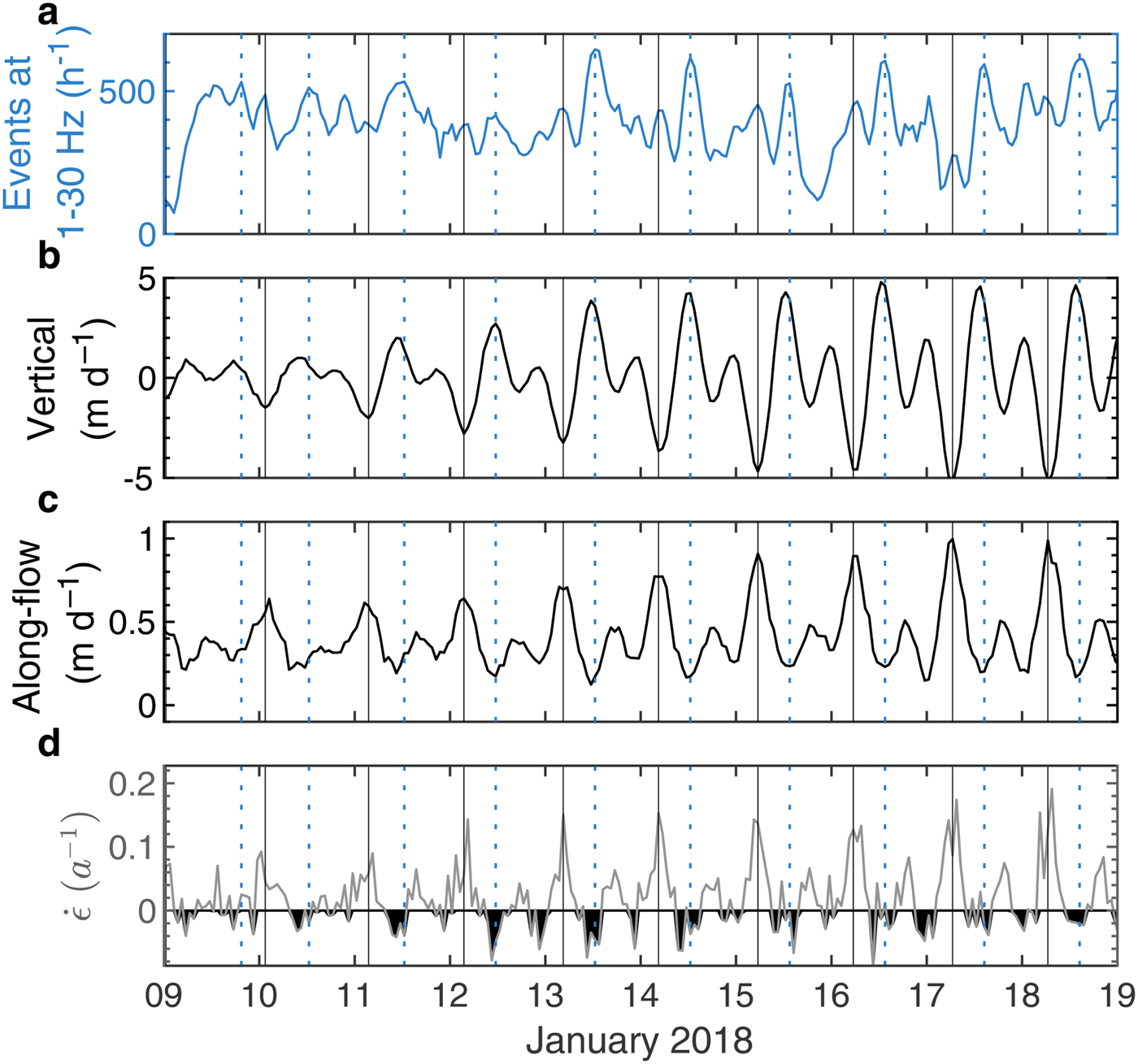
The low-frequency group exhibits a more pronounced increase in occurrence rate than the high-frequency group during mid-rising tides (Fig. 4). The waveforms of the low-frequency group might be similar to the previously reported hybrid icequakes observed at an Alaskan glacier (West and others, Reference West, Larsen, Truffer, O'Neel and LeBlanc2010), which have been considered as a mechanism to explain the icequakes in Antarctic ice shelves (Hammer and others, Reference Hammer, Ohrnberger and Schlindwein2015; Lombardi and others, Reference Lombardi2016). These hybrid icequakes have a high-frequency wave onset that is followed by low-frequency waves. They are explained in terms of a hypothetical new basal crevasse opening (high-frequency), which leads to resonance of water-filled crevasse (low-frequency). We observed similar waveforms, although with some differences. Our examples do not always consist of a clear high-frequency onset, which may be due to attenuation. For example, the event shown in Fig. 3a has some high-frequency content in the beginning, whereas this is not seen for the event in Fig. 3b. Fig. 8 shows that the main peaks in low-frequency seismicity are in phase with neither the along-flow speed nor the longitudinal strain rates. Furthermore, the main peaks take place at negative longitudinal strain rates, which imply compression along the flow direction, and therefore correspond to the least likely timing for the opening of surface crevasses. This interpretation is in line with our hypothesis of higher seismicity due to basal-crevasse opening during rising and high tides.
(a) The occurrence rates of the icequakes observed between 9 and 19 January (for traces bandpass-filtered between 1 and 30 Hz). The time evolution of (b) the vertical and (c) along-flow ice speed at LG1, and (d) the longitudinal strain rates between LG1 and LG2 (defined as  $\dot {\epsilon } = \partial s/\partial x$, where s is the along-flow speed and x is the distance). Negative strain rates are highlighted in black. Vertical blue dotted and black lines show the time of daily maxima in the icequakes and vertical speed, respectively.
The sample rate of the seismic signals in our study (400 Hz) was higher than that in previous Antarctic studies (Hammer and others, Reference Hammer, Ohrnberger and Schlindwein2015; Lombardi and others, Reference Lombardi2016; Pirli and others, Reference Pirli, Hainzl, Schweitzer, Köhler and Dahm2018), which enabled us to monitor high-frequency seismicity (Figs 3 and 4). We observed a larger number of icequakes in the high-frequency band (up to 800 events h−1) than in the low-frequency band (Fig. 4d). Furthermore, increased occurrence rates of these high-frequency events were observed during rising and high tides, with typical high-frequency, impulsive events (Figs 3c–e) corresponding to the statistics shown in Fig. 4d. When only considering the similarity in the high-frequency content, we note that such events were interpreted as deep or basal icequakes that were initiated by brittle tensile failure or hydrofracture on Alpine and Greenlandic glaciers (Walter and others, Reference Walter2009; Röösli and others, Reference Röösli2014). These studies reported that the waveforms were characterized by an impulsive first motion, with strong P- and S-phases and little or no Rayleigh waves. We acknowledge that detailed waveform analysis and waveform modeling might yield better constraints on their mechanisms. However, we hypothesize that these high-frequency events are likely related to brittle failure, with an englacial or basal origin, that are initiated in response to floating tongue bending.
Seismicity due to surface crevasses (minor peaks)
We observed an increase in seismic power in the low-frequency range (~10 Hz) during the falling tide that is coincident with the maximum ice flow speed (Fig. 8). The temporal variation in the occurrence rates of low-frequency seismicity also suggests the existence of minor peaks due to a higher number of events during the falling tides (Fig. 8a). This is also observed to a degree in the PSD-PDFs, as slightly elevated energy levels are observed at ~10 Hz (Fig. 5d). Compared with other PSD-PDFs, only the falling tides produce this relatively narrow, localized peak. There are two possible source mechanisms: i) basal friction along unknown pinning points (e.g., Pirli and others, Reference Pirli, Hainzl, Schweitzer, Köhler and Dahm2018) or near the grounding line due to the high ice flow speed (Aðalgeirsdóttir and others, Reference Aðalgeirsdóttir2008), and ii) surface cracking due to an enhanced longitudinal strain rate and tension due to vertical bending (Barruol and others, Reference Barruol2013; Podolskiy and others, Reference Podolskiy2016). Our GNSS measurements indicate that the vertical and along-flow ice flow speed and the longitudinal strain rate reach their maxima during the falling tide at Langhovde Glacier (Figs 2b and 8). The vertical ice speed is five times larger than the along-flow ice speed. The result suggests that the bending at falling tides could be the predominant mechanism to enhance surface crevassing. It is interesting to note that the maximum longitudinal strain rates do also correspond to the secondary peaks in seismicity, as highlighted by the vertical lines in Fig. 8. This suggests that the extensional motion of the glacier corresponds to the slightly intensified seismicity, but that it is of minor importance compared with the main seismicity bursts during rising and high tides. Our preliminary analysis points to surface crevassing as the most likely mechanism, but the alternative interpretation of basal friction cannot be ruled out.
CONCLUSIONS
We simultaneously deployed GNSS and passive seismic instruments on the floating glacier tongue of Langhovde Glacier, East Antarctica, for 2 weeks in January 2018. The period covered one neap to spring tides cycle. The vertical ice motion had an order of magnitude larger tidal admittance than the along-flow motion near the terminus. It decayed toward the grounding line, ~3 km up-glacier, with the along-flow motion of the glacier becoming more dominant. The maximum ice flow speed reaches its maximum during the falling tide, presumably due to the elastic response of the glacier following the reduction in hydrostatic stress acting on the floating glacier front.
We observed a range of icequake types across a broad frequency range, with occurrence rates up to 800 events h−1. The highest intensity of local icequake activity is observed during rising and high tides, which primarily correlated with the vertical ice motion. This covariance implies that a basal icequake origin due to floating tongue bending is the most likely source mechanism. This pattern is similar to the findings of Lombardi and others (Reference Lombardi2016), but different to the longitudinal-stretching mechanism proposed by Podolskiy and others (Reference Podolskiy2016) owing to the dominance of vertical glacier motion near the terminus.
Further analysis of this dataset in a follow-up study, via the implementation of more sophisticated detection/classification algorithms, location routines and waveform modeling, has the potential to better constrain the source mechanisms of the icequakes at Langhovde Glacier and understand their importance in the context of ice-shelf dynamics.
AUTHOR CONTRIBUTION
MM collected data, performed the analysis and wrote the paper. EP contributed to data analysis and to writing the paper. SS designed the field study at the glacier and contributed to writing the paper. All authors contributed to the discussion of the results.
ACKNOWLEDGMENTS
We thank Masato Ito, Shiori Yamane, Shinji Takamura, Tatsuro Tsuchiya, and the 58th and 59th Japanese Antarctic Research Expedition members for their assistance at Langhovde Glacier. We also thank Shigeru Aoki and Takeshi Tamura for their support to the research activity. The manuscript was handled by Scientific Editor, Fabian Walter, and carefully reviewed by two anonymous reviewers. This research was funded by Research of Ocean-ice BOundary InTeraction and Change around Antarctica (ROBOTICA) (2016–2022), JSPS KAKENHI on Innovative Areas Grant Number 4902 (2018–2022), and JSPS KAKENHI Grant Number 18K18175. Masahiro Minowa was supported by a JSPS Overseas Research Fellowship (#201860152, 2018–2020). GNSS and seismic signal were processed with RTKLIB (http://www.rtklib.com/rtklib.htm) and ObsPy (http://www.obspy.org), respectively. Figures were produced by Matlab and QGIS. The Landsat 8 image was downloaded from http://earthexplorer.usgs.gov/. Tide gauge and weather records at Syowa Station are available from the Intergovernmental Oceanographic Commission archive database (http://www.ioc-sealevelmonitoring.org) and Japanese Meteorological Agency (http://www.data.jma.go.jp). The Plèiades orthoimage and digital elevation model used in this study were provided by the Plèiades Glacier Observatory initiative of the French Space Agency (CNES).


 Open access