2. The numerical dataset

The DNS solver relies on a second-order finite-difference discretisation of the incompressible Navier–Stokes equations in cylindrical coordinates, utilising the marker-and-cell method to maintain discrete conservation of the total kinetic energy (Orlandi Reference Orlandi2000). To ensure a constant mass flow rate, uniform volumetric forcing is applied to the axial momentum equation. The Poisson equation resulting from enforcement of the divergence-free condition is efficiently solved through double trigonometric expansion in periodic axial and azimuthal directions, coupled with tridiagonal matrix inversion in the radial direction (Kim & Moin Reference Kim and Moin1985). The polar singularity at the pipe axis is handled as suggested by Verzicco & Orlandi (Reference Verzicco and Orlandi1996). Time advancement relies on a hybrid third-order low-storage Runge–Kutta algorithm, whereby diffusive terms are treated implicitly and convective terms are treated explicitly. Implicit treatment of the convective terms in the azimuthal direction is also used to mitigate the time-step restriction (Akselvoll & Moin Reference Akselvoll and Moin1996; Wu & Moin Reference Wu and Moin2008). The code is optimised for GPU clusters using CUDA Fortran and OpenACC directives, with CUFFT libraries facilitating fast Fourier transforms (Fatica & Ruetsch Reference Fatica and Ruetsch2014).

A sketch of the computational domain is shown in figure 1. The radial coordinate measured from the pipe axis is denoted as $r$. Numerical simulations are carried out using periodic boundary conditions in the axial ($z$) and azimuthal ($\theta$) directions. The effect of rotation is accounted for by augmenting the Navier–Stokes equations with the Coriolis forces:

(2.1) \begin{equation} \boldsymbol{F}_c = 2 \varOmega \left[ \begin{array}{@{}c@{}} - u_z \sin \theta \\ u_z \cos \theta \\ u_{r} \cos \theta - u_{\theta} \sin \theta \\ \end{array} \right] , \end{equation}

where the angular velocity ($\varOmega$) is assumed to be parallel to the polar ($x_2$) axis. The wall distance is hereafter denoted as $y$. As noted in previous studies, centrifugal forces are not explicitly added as they are absorbed into the pressure term (Kristoffersen & Andersson Reference Kristoffersen and Andersson1993). As illustrated in figure 1, the primary effect of rotation normal to the pipe axis is the onset of Coriolis forces which on average act orthogonal to both the pipe axis and the rotation axis, resulting in increased shear at the pressure side of the pipe and in shear suppression at the suction side. The flow is controlled by two parameters, namely the bulk Reynolds number, $\textit {Re}_b = 2 R u_b /\nu$, and the rotation number, $N=\varOmega R / u_b$, with $R$ the pipe radius, $u_b$ the bulk velocity and $\nu$ the fluid kinematic viscosity. This definition is used here as it emphasises the maximum peripheral velocity with respect to the bulk velocity, but one should be careful and note that several previous studies of rotating ducts rather define the rotation number based on the hydraulic diameter, here the pipe diameter. The friction Reynolds number $\textit {Re}_\tau$ is also an important flow parameter, defined as $\textit {Re}_\tau = R u^*_\tau /\nu$, with $u^*_\tau =(\tau ^*_w/\rho )^{1/2}$ the global friction velocity and $\tau ^*_w$ the azimuthally averaged mean wall shear stress. The flow properties normalised by these global viscous scales are hereafter denoted with an asterisk. In all DNS the pipe length is taken to be $L_z = 15 R$, which we have found to be sufficient to achieve convergence of all the statistics herein reported, as shown in the Appendix. The grid points are clustered towards the pipe walls according to the stretching function developed by Pirozzoli & Orlandi (Reference Pirozzoli and Orlandi2021), whereas the grid points are uniformly spaced in the $z$ and $\theta$ directions. Adequacy of the grid resolution has been evaluated through a grid sensitivity analysis, also reported in the Appendix.

Figure 1.

Definition of coordinate system for DNS of rotating pipe flow. Coordinates $z, r, \theta$ are the axial, radial and azimuthal coordinates, respectively, $R$ is the pipe radius, $L_z$ is the pipe length, $u_b$ is the bulk velocity, $\boldsymbol {\varOmega }$ is the angular velocity and $\boldsymbol {F}_c$ is the resultant mean Coriolis force. The Cartesian coordinates $x_1,x_2$ define positions in the cross-stream plane.

A complete list of the simulations that we have carried out is given in table 1. A one-decade range of Reynolds numbers has been explored, along with a wide range of rotation numbers, including cases with weak rotation as well as cases in which rotation dominates. For the sake of clarity, uppercase letters are used to denote flow properties averaged along the axial direction and in time, and fluctuations thereof are denoted with lowercase letters. Instantaneous properties are denoted with tilde superscripts. Angular brackets are used to denote the averaging operator.

Table 1.

Flow parameters for DNS of rotating pipe flow. The bulk Reynolds number is defined as $\textit {Re}_b = 2 R u_b/\nu$, with $R$ the pipe radius, $u_b$ the bulk velocity and $\nu$ the fluid kinematic viscosity; $N = \varOmega R/u_b$ is the rotation number and $N_\tau = \varOmega R/u^*_{\tau }$ is the friction rotation number with the global friction velocity. Parameters $N_z, N_r, N_\theta$ are respectively the number of grid points in the axial, radial and azimuthal directions. The parameter $N_{5\varDelta }$ highlights the number of points in the radial direction up to five Ekman layer thicknesses $\varDelta = (\nu /\varOmega )^{1/2}$, evaluated at $\theta = \pm 90^\circ$. The global friction factor is $\lambda = 8 \tau _w^* / \rho u_b^2$, with $\tau _w^*$ the azimuthally averaged mean wall shear stress and $\rho$ the fluid density. Parameter $\textit {Re}_{\tau } = R u^*_{\tau } / \nu$ is the friction Reynolds number, with $u^*_{\tau } = (\tau _w^*/\rho )^{1/2}$ the mean friction velocity.

3. Flow organisation

As a first step, we analyse the flow organisation from representative instantaneous snapshots at the two extreme Reynolds numbers, namely $\textit {Re}_b=17\,000$ and $\textit {Re}_b=133\,000$. Specifically, in figures 2 and 3 we show the contours of the axial velocity in the cross-stream plane and in figures 4 and 5 we show the axial velocity contours in a cylindrical shell at small distance ($\kern0.7pt y^*=15$ for the non-rotating case) from the wall. The former are used to get insight into the large-scale bulging motions which connect the near-wall region with the bulk flow, whereas the latter are used to get insight into the modifications of the near-wall streaks resulting from pipe rotation. For the sake of correct interpretation of the figures, we note that the azimuth angle $\theta$ as defined in figure 1 is such that $\theta =0^{\circ } \pm 15^\circ$ corresponds to the suction side of the pipe, whereas $\theta =180^{\circ } \pm 15^\circ$ corresponds to pressure side. Coriolis forces are such that on average momentum is transported from the suction side towards the pressure side (Zhang & Wang Reference Zhang and Wang2019). The angles $\theta = 90^{\circ }$ and $270^{\circ }$ correspond to the north and south poles of the pipe, respectively, along which the effects of rotation are most active. The first important information gained from the visualisations is that, even at modest rotation number (less that about $0.01$) the effect of rotation is quite apparent on the suction side, which shows a visible momentum defect with respect to the pressure side. Bulging motions are instead still observed on the rest of the pipe perimeter. As the rotation number increases, the zone with reduced momentum at the suction side of the pipe becomes progressively more extended, and severe reduction of the turbulence activity is visible at $N \gtrsim 0.1$. At higher rotation numbers suppression of turbulence is also visible within the pipe core, and hints of flow relaminarisation become visible also on the pressure side at $N \gtrsim 1$. Eventually, at high rotation rates, the flow tends to become symmetric about the polar axis, and the velocity field tends to become organised in bands parallel to it. The relaminarisation process is best observed in the near-wall shells. At low rotation numbers streaks dominate the near-wall region, although some evidence for their local suppression at $\theta \approx 0^{\circ }$ is visible. At intermediate rotation numbers streaks become progressively confined about the poles of the pipe, and they tend to vanish on the pressure side as well. At high rotation numbers, the flow no longer shows any sign of turbulence activity (please see supplementary movies at: https://doi.org/10.1103/APS.DFD.2023.GFM.V0041).

Figure 2.

Instantaneous axial velocity contours at $\textit {Re}_b = 17\,000$ in the cross-stream plane. Contour levels ranging from 0 to 1.4 are shown, in colour scale from blue to red. The pressure side of the pipe is on the left and the suction side is on the right of each panel. Various rotation numbers are considered: (a) $N = 0.0078125$, (b) $N = 0.125$, (c) $N = 0.25$, (d) $N = 0.5$, (e) $N = 2.0$, (f) $N = 8.0$.

Figure 3.

Instantaneous axial velocity contours at $\textit {Re}_b = 133\,000$ in the cross-stream plane. Contour levels ranging from 0 to 1.4 are shown, in colour scale from blue to red. The pressure side of the pipe is on the left and the suction side is on the right of each panel. Various rotation numbers are considered: (a) $N = 0.01$, (b) $N = 0.5$, (c) $N = 16.0$.

Figure 4.

Instantaneous axial velocity contours at $\textit {Re}_b = 17\,000$ in an unrolled cylindrical shell at a distance $y^*=15$ from the wall (evaluated in the non-rotating case). Contour levels ranging from 0 to 1.4 are shown, in colour scale from blue to red. The insets in the top-right corner of each panel report magnified views of a small portion of the shell. Various rotation numbers are considered: (a) $N = 0.0078125$, (b) $N = 0.25$, (c) $N = 0.5$, (d) $N = 8.0$.

Figure 5.

Instantaneous axial velocity ($u_z/u_b$) at $\textit {Re}_b = 133\,000$ in an unrolled cylindrical shell at a distance $y^*=15$ from the wall (evaluated in the non-rotating case). Contour levels ranging from 0 to 1.4 are shown, in colour scale from blue to red. The insets in the top-right corner of each panel report magnified views of a small portion of the shell. Various rotation numbers are considered: (a) $N = 0.01$, (b) $N = 0.5$, (c) $N = 2.0$, (d) $N = 16.0$.

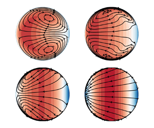
Since the flow exhibits homogeneity in the axial direction, its statistical characteristics solely rely on the azimuthal and radial coordinates. The mean axial velocity within the cross-stream plane is depicted in figure 6 for flow cases with $\textit {Re}_b=17\,000$, at various rotation numbers. Representative cross-flow streamlines are superimposed to the velocity contours to emphasise the variations in secondary motions as the rotation number changes. At low-to-moderate $N$ (figure 6a–d), a notable alteration involves the symmetry breaking with respect to the polar axis, which implies gradual increase of axial momentum on the pressure side of the pipe (left) and a decrease on the suction side (right), on account of Coriolis forces. Consequently, secondary motions emerge in the form of two counter-rotating eddies that facilitate momentum redistribution across the pipe cross-section, with primary flow moving from the suction to the pressure side along the horizontal symmetry axis and return motion occurring along the circumference of the pipe. Remarkably, at low $N$, these secondary motions closely resemble those predicted to form under laminar flow conditions (Barua Reference Barua1954). As the rotation number increases, there is a discernible trend towards uniformity in mean velocity along the vertical direction, accompanied by a tendency for the momentum deficit at the suction to be compensated, resulting in symmetrisation of the flow field. This observed phenomenon distinctly marks the onset of Taylor–Proudman columns (Proudman Reference Proudman1916; Taylor Reference Taylor1917), characterised by a tendency for the velocity to be constant along the axis of rotation, with no tilting or stretching of material lines parallel to this axis. At extreme rotation numbers, the secondary motions correspondingly take the form of right-to-left cross-stream motion, with return motions barely noticeable and confined to the near-wall proximity. Identical cross-stream flow information is presented in figure 7 for flow cases with $\textit {Re}_b = 133\,000$. A remarkably similar flow pattern is discerned at corresponding values of the rotation number, for instance, comparing figure 6(a,d) with figure 7(a,b). This observation reinforces the idea that rotational effects on the mean flow properties are relatively unaffected by changes in the flow Reynolds number.

Figure 6.

Mean axial velocity contours with superposed cross-flow streamlines, at $\textit {Re}_b = 17\,000$. Twenty-four contour levels ranging from 0 to 1.4 are shown, in colour scale from blue to red. The pressure side of the pipe is on the left and the suction side is on the right of each panel. Various rotation numbers are considered: (a) $N = 0.0078125$, (b) $N = 0.125$, (c) $N = 0.25$, (d) $N = 0.5$, (e) $N = 2.0$, (f) $N = 8.0$.

Figure 7.

Mean axial velocity contours with superposed cross-flow streamlines, at $\textit {Re}_b = 133\,000$. Twenty-four contour levels ranging from 0 to 1.4 are shown, in colour scale from blue to red. The pressure side of the pipe is on the left and the suction side is on the right of each panel. Various rotation numbers are considered: (a) $N = 0.01$, (b) $N = 0.5$, (c) $N = 16.0$.

Due to the rearrangement of the flow, significant changes occur in wall friction as $N$ varies. To examine this effect, figure 8 illustrates the local streamwise wall shear stress, $\tau _w/\rho = \nu \partial U_z/ \partial y|_w$, normalised either by the reference dynamic pressure $\rho u_b ^2$ (figure 8a,c) or the mean wall shear stress $\tau _w^*$ (figure 8b,d). A polar diagram is employed for clarity. The figure clearly demonstrates that even at very low rotational speeds, friction is nearly completely suppressed at the suction side of the pipe ($\theta =0$). Conversely, the behaviour on the pressure side ($\theta ={\rm \pi}$) is non-monotonic, where the local streamwise wall shear stress initially increases due to local acceleration of the bulk flow, then abruptly declines beyond $N \approx 1$, signifying the dominance of rotation and the concentration of momentum around the vertical axis of the pipe. Friction at the poles of the pipe ($\theta =90^{\circ }, 270^{\circ }$) exhibits a monotonically increasing trend with the rotation number, on account of local thinning of the boundary layer, as detailed further ahead. At higher values of $N$ considered, the local friction tends to attain a universal distribution when scaled by its mean value, regardless of the Reynolds number.

Figure 8.

Polar distribution of the local streamwise wall shear stress ($\tau _w$), normalised by either the reference dynamic pressure $\rho u_b ^2$ (a,c) or the mean wall shear stress $\tau _w^*$ (b,d), at $\textit {Re}_b=17\,000$ (a,b) and $\textit {Re}_b=133\,000$ (c,d). The colour codes correspond to different values of $N$, as given in table 1, grey denoting cases without rotation. The dashed blue line in (a,c) denotes the predictive formula given in (5.4).

The mean axial velocity profiles are shown in outer scaling in figure 9. For the sake of clarity, the radial profiles are shown in the interval $\theta =[0,90^{\circ }]$ along the pipe perimeter. Due to flow symmetry, this interval is sufficient to fully describe the state of the axial velocity in the pipe. The axial velocity for the non-rotating case ($N=0$) is also reported for reference, which is obviously symmetric. As rotation sets in, the velocity profile along the horizontal symmetry axis (in orange shades) is immediately broken, and the peak value is shifted from the pipe centre to the pressure side of the pipe due to the presence of secondary motions in the cross-stream direction. The tendency of the axial velocity peak to shift towards the pressure side of the pipe is, however, non-monotonic. As the rotation number approaches unity, in fact the peak value of the axial velocity moves back towards the centre of the pipe, as shown in figure 9(b–d), and the velocity profiles again become symmetric with respect to the origin. As for the velocity profiles along the polar direction (in purple shades), they show a sudden tendency to flatten out in the middle of the pipe, whereas peaks tend to arise towards the pipe walls, which are associated with the formation of Ekman layers due to rotation. This tendency is exacerbated at high $N$, at which the mean axial velocity is very nearly constant throughout the vertical axis of the pipe, and gradients become progressively restricted to the near-wall vicinity. This change in the flow structure is clearly related to the onset of Taylor–Proudman columns previously noted when discussing figure 6. The same changes in the flow behaviour are also observed at $\textit {Re}_b=133\,000$ (figure 9(e–h). However, when comparing cases with the same vale of $N$ (e.g. figures 9b and 9f), one can observe that the tendency for the flow to become symmetric about the vertical axis is faster at higher $\textit {Re}_b$, whereas the Ekman layers are visually thinner at the higher $\textit {Re}_b$.

Figure 9.

Radial profiles of outer-scaled axial velocity at various azimuthal positions, for flow cases at $\textit {Re}_b=17\,000$ (a–d) and $\textit {Re}_b=133\,000$ (e–h). Only the interval $\theta = [0^{\circ },90^{\circ }]$ is shown, at stations spaced $7.5^\circ$ apart, with negative values of $r$ signifying profiles taken at $\theta + 180^{\circ }$. Values of (a) $N = 0.03125$, (b) $N = 0.5$, (c) $N = 2.0$, (d) $N = 8.0$, (e) $N = 0.1$, (f) $N = 0.5$, (g) $N = 2.0$, (h) $N = 16.0$. The black solid line denotes the mean axial velocity profile in the non-rotating case.

It is important to recognise the substantial difference of the present flow arrangement with respect to the case of a spanwise rotating channel which was considered by Kristoffersen & Andersson (Reference Kristoffersen and Andersson1993). In that case the Taylor–Proudman columns that would form at high rotation rates would be aligned with the spanwise direction, parallel to the rotation axis. Hence, they would not interact with solid walls and give rise to Ekman layers, which in the flow case under scrutiny here are chiefly responsible for drag increase around the north and south poles, as figure 8 shows.

Figure 10 reports representative wall-normal axial velocity profiles in local wall units (i.e. based on the local friction velocity $u_{\tau }=(\tau _w/\rho )^{1/2}$) as a function of the wall distance, to highlight deviations from the universal law of the wall which is observed in non-rotating pipe flow. For the sake of clarity, the velocity profiles are shown up to the occurrence point of their first maximum. The figure shows that the velocity distributions on the suction side (orange shades) become immediately diverted from the logarithmic behaviour, highlighting a clear decrease of the local friction. The velocity profiles on the pressure side (in cyan shades) are more resilient to the effect of rotation, and a logarithmic layer is still observed at low rotation numbers. At intermediate rotation numbers, the logarithmic part of the velocity profiles is shifted downwards, indicating an increase of the local friction, until the logarithmic layer becomes entirely disrupted at $N \gtrsim 1$. As seen in Figure 10(e–h), an increase of the Reynolds number mainly implies greater robustness of the logarithmic behaviour, which persists until $N \approx 1$ at $\textit {Re}_b=133\,000$.

Figure 10.

Wall-normal profiles of inner-scaled axial velocity, at various azimuthal positions spaced $7.5^\circ$ apart, for flow cases at $\textit {Re}_b=17\,000$ (a–d) and $\textit {Re}_b=133\,000$ (e–h). Only the interval $\theta = [0^{\circ },180^{\circ }]$ is shown. Values of (a) $N = 0.03125$, (b) $N = 0.5$, (c) $N = 2.0$, (d) $N = 8.0$, (e) $N = 0.1$, (f) $N = 0.5$, (g) $N = 2.0$, (h) $N = 16.0$. The black solid line denotes the mean axial velocity profile in the non-rotating case. The dashed grey lines depict the compound law of the wall $U^+=y^+$, $U^+=\log y^+/0.387 + 4.53$.

Yang et al. (Reference Yang, Xia, Lee, Lv and Yuan2020) argued that, for a channel that rotates about its spanwise axis at a reasonably high speed, the mean flow near the pressure side should follow a linear scaling, i.e.

(3.1)\begin{equation} U_z^+= 2 \frac {\varOmega y}{u_{\tau}} + C, \end{equation}

with additive constant

(3.2)\begin{equation} C = \frac 1{\kappa} \log \left( \frac {u_{\tau}^2}{\nu \varOmega} \right). \end{equation}

This prediction is compared with the DNS data in figure 11, where we have assumed $\kappa = 0.33$. We find that the scaling holds with reasonable accuracy for cases with intermediate rotation rate, specifically for $N=0.25,0.5$ at $\textit {Re}_b = 17\,000$ and for $N=0.5,2.0$ at $\textit {Re}_b=133\,000$, but it clearly fails at high rotation rates as the flow relaminarises.

Figure 11.

Inner-scaled wall-normal mean velocity profiles at $\theta = 180^\circ$ (pressure side). Solid lines refer to DNS data and dashed lines to (3.1), for flow cases at $\textit {Re}_b = 17\,000$ (a) and cases at $\textit {Re}_b = 133\,000$ (b). Colour codes are as in table 1.

The statistics of the turbulence kinetic energy ($k = \langle u_i u_i \rangle /2$) are examined in figure 12. As for the mean velocity, we find that axial symmetry observed in non-rotating cases is broken in the presence of weak rotation. At low rotation numbers (figure 12a) the magnitude of the buffer-layer peak along the horizontal symmetry axis of the pipe (orange shades) increases on the pressure side and decreases on the suction side, in response to increase and decrease of the imposed shear, respectively. Relaminarisation of the flow occurs on the suction side of the pipe already at $N \approx 0.125$. The buffer-layer peaks along the polar direction (purple shades) are instead barely affected. The most notable feature in the weak rotation regime is the reduction and flattening of $k$ in the interior part of the pipe. This tendency becomes most evident as $N$ increases, with suppression of the turbulence kinetic energy in the entire flow field, at $N \gtrsim 2$. A similar scenario is also found at higher $\textit {Re}_b$ (figure 12e–h), at which, however, some signs of turbulence activity are still visible at the pressure side, even at $N=2$ (figure 12g). The flow is found to be fully laminar at $N=16$.

Figure 12.

Radial profiles of outer-scaled turbulence kinetic energy at various azimuthal positions, for flow cases at $\textit {Re}_b=17\,000$ (a–d) and $\textit {Re}_b=133\,000$ (e–h). Only the interval $\theta = [0^{\circ },90^{\circ }]$ is shown, at stations spaced $7.5^\circ$ apart, with negative values of $r$ signifying profiles taken at $\theta + 180^{\circ }$. Values of (a) $N = 0.03125$, (b) $N = 0.5$, (c) $N = 2.0$, (d) $N = 8.0$, (e) $N = 0.1$, (f) $N = 0.5$, (g) $N = 2.0$, (h) $N = 16.0$. The black solid line denotes the mean turbulence kinetic energy profile in the non-rotating case.

As noted when discussing figure 9, starting from rotation numbers of the order of unity, the flow exhibits the clear hallmark of Ekman layers, namely thin layers in which the direction of the wall-parallel velocity changes as a result of varying relative importance of imposed pressure gradient, Coriolis and viscous forces. The laminar Ekman solution for rotating flow over a flat wall reads (Greenspan Reference Greenspan1968)

(3.3a)$$\begin{gather} \frac{U_z (y)}{U_{g}} = 1 - {\rm e}^{{-}y/\varDelta} \cos \left( \frac{y}{\varDelta} \right), \end{gather}$$

(3.3b)$$\begin{gather}\frac{U_{\theta} (y)}{U_{g}} = {\rm e}^{{-}y/\varDelta} \sin \left( \frac{y}{\varDelta} \right), \end{gather}$$

where $y$ is the wall distance, $U_g$ is the intensity of the asymptotic (geostrophic) wind and $\varDelta = (\nu /\varOmega )^{1/2}$ is the thickness of the Ekman layer. The Ekman layer in the vicinity of the north pole of the pipe (namely $\theta = 90^{\circ }$) is analysed in figure 13, where the wall distance is scaled with respect to the Ekman length scale, and the geostrophic wind intensity is assumed to be the mean velocity at the pipe centreline, say $U_0$. The individual axial and azimuthal velocity components are shown in figure 13(a), the flow angle with respect to the axial direction is shown in figure 13 (b) and the projection in the hodograph plane is shown in figure 13 panel (c). As the rotation number increases the figure shows the onset of an overshoot of the axial velocity and the presence of a non-zero azimuthal velocity component. As a consequence, the flow becomes diverted from the axial direction, to an extent which is proportional to $N$. Excellent agreement between the computed profiles at high values of the rotation number and the theoretical prediction given in (3.3) is found. This is in our opinion a rather remarkable result, as the laminar Ekman solution is derived for the case of wall-normal rotation over a flat wall. Here, we find that it also applies with excellent accuracy to flow over a curved surface, with an effective rotation rate given by the wall-normal projection of the angular velocity vector. The same arguments apply for the highest tested Reynolds number (see figure 14), for which a laminar Ekman layer is found at $N=16$.

Figure 13.

Profiles of mean axial ($U_z$) and azimuthal ($U_\theta$) velocity (a), wall-parallel flow angle $\varphi = \tan ^{-1} (U_{\theta }/U_z)$ (b) and hodograph diagram (c) at the polar coordinate $\theta = {\rm \pi}/2$ (north pole of the pipe). Data are shown for $\textit {Re}_b=17\,000$, at various rotation numbers: $N = 0.03125$, $N = 0.0625$, $N = 0.125$, $N = 0.25$, $N = 0.5$, $N = 2.0$, $N = 4.0$, $N = 8.0$. See table 1 for the colour codes. The velocity profiles are scaled by the mean centreline axial velocity $U_{0}$. The black circles denote the analytical solution for a laminar Ekman layer (Greenspan Reference Greenspan1968).

Figure 14.

Profiles of mean axial ($U_z$) and azimuthal ($U_\theta$) velocity (a), wall-parallel flow angle $\varphi = \tan ^{-1} (U_{\theta }/U_z)$ (b) and hodograph diagram (c) at the polar coordinate $\theta = {\rm \pi}/2$ (north pole of the pipe). Data are shown for $\textit {Re}_b=133\,000$, at various rotation numbers: $N = 0.1$, $N = 0.5$, $N = 2.0$, $N = 16.0$. See table 1 for the colour codes. The velocity profiles are scaled by the mean centreline axial velocity $U_{0}$. The black circles denote the analytical solution for a laminar Ekman layer (Greenspan Reference Greenspan1968).

4. Friction

Frictional drag in pipes is obviously a parameter of paramount importance as it is related to power expenditure to sustain the flow. Whereas accurate estimates of friction are available for pressure-driven pipe flow, the presence of imposed rotation has profound effects on the structure of turbulence and the onset of secondary motions, which were pinpointed in the previous section. In order to isolate the contributions of turbulence, secondary motions and rotation to frictional drag, here we consider a generalised version of the FIK identity (Fukagata, Iwamoto & Kasagi Reference Fukagata, Iwamoto and Kasagi2002), which was derived for flow in ducts with arbitrary cross-section (Modesti et al. Reference Modesti, Pirozzoli, Orlandi and Grasso2018). The starting point is the mean momentum balance equation, which reads

(4.1)\begin{equation} \nu \nabla ^2 U_z ={-} \varPi + \boldsymbol{\nabla} \boldsymbol{\cdot} \boldsymbol{\tau_T} + \boldsymbol{\nabla} \boldsymbol{\cdot} \boldsymbol{\tau_C} + F_{c,z}, \end{equation}

where $\varPi$ is the driving pressure gradient, $\boldsymbol {\tau _T} = \langle u_z \boldsymbol {u_{r \boldsymbol {\theta }}} \rangle$ accounts for turbulent convection ($\boldsymbol {u_{r \theta }}= (u_r, u_\theta )$ is the cross-stream velocity vector), $\boldsymbol {\tau _C} = U_z \boldsymbol {U_{r \boldsymbol {\theta }}}$ accounts for mean cross-stream convection (hence, with the secondary motions) and $F_{c,z}$ is the axial component of the Coriolis forces given in (2.1). Equation (4.1) may be regarded as a Poisson equation for $U_z$ velocity whose source terms can be obtained from DNS data. Hence, the mean streamwise velocity field can be cast as a superposition of four contributions, which individually satisfy

(4.2a–d)\begin{equation} \nabla ^2 U_{zV} ={-} \varPi, \quad \nabla ^2 U_{zT} = \boldsymbol{\nabla} \boldsymbol{\cdot} \boldsymbol{\tau_T}, \quad \nabla ^2 U_{zC} = \boldsymbol{\nabla} \boldsymbol{\cdot} \boldsymbol{\tau_C}, \quad \nabla ^2 U_{zR} = F_{c,z}, \end{equation}

with homogeneous boundary conditions, from viscous effects ($V$), from turbulence ($T$), from mean cross-stream convection ($C$) and from rotation ($R$). The bulk velocity can then be obtained as the superposition of four terms,

(4.3)\begin{equation} u_b = u_{bV} + u_{bT} + u_{bC} + u_{bR}, \end{equation}

each denoting the mean value associated with the four velocity fields defined in (4.2a–d). Using (4.3) in the definition of the friction factor one obtains

(4.4)\begin{equation} \lambda = \frac{8 \tau_w ^*}{\rho u_{bV} u_{b}} \left ( 1 - \frac{u_{bT}}{u_b} - \frac{u_{bC}}{u_b} - \frac{u_{bR}}{u_b} \right ) = \lambda_{V} + \lambda_{T} + \lambda_{C} + \lambda_{R}, \end{equation}

where the viscous contribution ($\lambda _V=64/\textit {Re}_b$) corresponds to the case of laminar flow. This information has major importance as it allows one to highlight the key physical mechanisms for friction generation depending on the pipe rotation rate. Notably, (4.4) reverts to the classical FIK identity in the case of canonical plane channel and circular pipe flow, in the absence of rotation. It is important to acknowledge that the FIK identity cannot be strictly intended as a tool to precisely isolate causality links in the flow. For instance, it is clear that secondary motions in circular pipe flow would not form in the absence of rotation, and that rotation causes a change in the structure of turbulence. Nevertheless, the generalised form of the FIK identity as here introduced is useful as it provides quantitation of the friction contributions from the various terms appearing in the mean momentum balance equation, thus allowing one to identify distinct flow regimes depending on their relative importance.

Figure 15 shows the contributions to the mean friction factor in both relative and absolute terms. According to (4.4), the absolute viscous contribution to the friction factor does not change with $N$, hence its relative contribution decreases monotonically. As regards the turbulent contribution, in non-rotating cases it increases from 86 % (at $\textit{Re} _b=17\,000$) to 97 % (at $\textit{Re} _b=133\,000$), and it monotonically decreases with $N$, becoming negligible at $N \gtrsim 1$. At the lower $\textit {Re}$, for which several data points are available at low $N$, we see that the contributions to friction are basically identical to those for the non-rotating case up to $N \approx 0.001$. The contribution from the secondary motions has a non-monotonic behaviour being nearly zero in the two extreme cases of non-rotating and rapidly rotating flow, whereas it accounts for as much as 50 % in the intermediate rotation regimes ($0.01 \leqslant N \leqslant 0.1$). The distributions are also very similar at the two Reynolds numbers reported in the figure, although $\lambda _C$ is found to become slightly negative at the higher $\textit {Re}$. This similarity might suggest that $N$ is an appropriate parameter to quantify the importance of secondary motions in radially rotating pipe flow. Monotonic growth of the contribution due to rotation is observed, with weak sensitivity to the Reynolds number. In quantitative terms, rotation accounts for almost 40 % of the total friction for $N \approx 0.1$, and it is responsible for at least 80 % of friction at $N \gtrsim 1$.

Figure 15.

Contributions to friction factor ($\bullet$) from viscous effects (${\bf {+}}$), turbulence ($\boldsymbol {*}$), mean cross-stream convection ($\bigstar$) and rotation ($\blacksquare$), as defined in (4.4). Percentage contributions are shown as a function of $N$ in (a,c) and absolute contributions are shown as a function of $(N/\textit {Re}_b)^{1/2}$ in (b,d), for $\textit {Re}_b = 17\,000$ (a,b) and $\textit {Re}_b = 133\,000$ (c,d).

5. Friction estimates

Based on the results of the previous section, herein we attempt to derive predictive formulas for the friction coefficient as a function of the controlling parameters, namely Reynolds and rotation numbers. Preliminarily, we consider the two limiting cases of no rotation ($N=0$) and rapid rotation ($N \gg 1$). In the former case, the Prandtl friction law for smooth pipes is known to perform very well, namely

(5.1)\begin{equation} 1 / \lambda_0 ^{1/2} = A \log_{10} \left( \textit{Re}_b \lambda_0 ^{1/2} \right) - B, \end{equation}

where $\lambda _0$ is the friction factor for the non-rotating case at a given $\textit {Re}_b$, and $A \approx 2.102$, $B \approx 1.148$, as obtained from fitting DNS data (Pirozzoli et al. Reference Pirozzoli, Romero, Fatica, Verzicco and Orlandi2021).

In the opposite case of rapid rotation an approximate theoretical treatment is possible as the flow tends to become fully laminar. As a first step for that purpose, we recall that analysis of the mean velocity maps in figures 6 and 7 shows that, with the exception of the near-wall Ekman layers, the mean axial velocity becomes solely a function of the horizontal direction as a result of the Taylor–Proudman theorem. Hence, in figure 16 we show a scatter plot of the mean axial velocity as a function of the horizontal coordinate ($x_1=r \cos \theta$), after removing points closer to the wall than $5 \varDelta$, which roughly corresponds to the effective thickness of the Ekman layer. The figure shows that, regardless of the Reynolds number, all data points fall on the same distribution, thus corroborating the initial assumption. Furthermore, we find that a convenient fit for the axial velocity distribution is as follows:

(5.2)\begin{equation} \frac{U_{z,e} (r, \theta)}{u_b} = A \left[ 1-\left( \frac{r}{R} \right)^2 \cos^2 \theta \right]+B \left[ 1-\left( \frac{r}{R} \right)^2 \cos^2 \theta \right]^2, \end{equation}

with $A=1.74$ and $B=-0.484$ as determined from fitting the DNS data, which also lends itself to simple mathematical manipulations. Lack of perfect symmetry in figure 16 is rather apparent, which could be incorporated in (5.2); however, the practical impact of such corrections on the overall friction would be minimal.

Figure 16.

Scatter plots of mean axial velocity as a function of the horizontal coordinate, for $\textit {Re}_b=17\,000, N = 8$ (a) and $\textit {Re}_b=133\,000, N = 16$ (b), in blue. Only points at wall distance greater than five Ekman layer thicknesses are shown. The black dashed lines denote the velocity profile given in (5.2).

As for the mean axial velocity profiles within the Ekman layer, (3.3a) is adapted to the present case by assuming that: (i) the local effective angular velocity at a given azimuthal angle is the wall-normal component, namely $\varOmega \sin \theta$, and (ii) the effective geostrophic velocity is the wall-limiting value of the mean velocity distribution in the pipe core, as given in (5.2); hence we set $U_g(\theta ) = U_{z,e} (R, \theta )$.

These assumptions are scrutinised in figure 17, where we shown the mean axial velocity profiles as a function of the wall distance, scaled respectively by the assumed geostrophic velocity and by the local Ekman layer thickness. Several profiles along the pipe perimeter are shown, with the exception of those at $\theta =0^{\circ }$ and $\theta =180^{\circ }$, where $U_{z,e} = 0$. The cases with highest rotation numbers for each extreme Reynolds number are reported in the figure. The figure confirms that the local Ekman layer thickness ($\varDelta = (\nu /(\varOmega \sin \theta ))^{1/2}$) is the correct length scale for the velocity profiles, as it yields universality of the velocity overshoot point, which occurs at $y \approx 2.3 \varDelta$, regardless of the azimuthal positions. Whereas the profiles near the north pole, $\theta =90^{\circ }$, exhibit perfect agreement with the canonical Ekman solution, good agreement is also observed at all azimuthal positions.

Figure 17.

Mean axial velocity profiles scaled by the local geostrophic velocity ($U_g$) as a function of wall distance normalised by the local Ekman layer thickness, $\varDelta = (\nu /(\varOmega \sin \theta ))^{1/2}$, at $\textit {Re}_b=17\,000$, $N=8$ (a) and $\textit {Re}_b=133\,000$, $N=16$ (b). Profiles along the pipe perimeter are shown in intervals of $7.5^{\circ }$, with the exception of $\theta =0^{\circ }$ and $\theta =180^{\circ }$.

A prediction for the distribution of the wall friction along the pipe perimeter is then obtained from (3.3a), which upon differentiation at the wall yields

(5.3)\begin{equation} \frac{\tau_w}{\rho} = \left.\nu \frac{\mathrm{d}U_{z}}{\mathrm{d}y} \right|_{y=0} = \nu \frac{U_{z,e}(R, \theta)}{(\nu / (\varOmega \sin \theta))^{1/2}}. \end{equation}

Using (5.2) to determine the geostrophic velocity one then obtains

(5.4)\begin{equation} \tau_w = 2^{1/2} \rho u_b ^2 (\sin \theta)^{1/2} \left( \frac{N}{\textit{Re}_b} \right)^{1/2} \left[ A \left( 1- \cos^2 \theta \right)+ B \left( 1- \cos^2 \theta \right)^2 \right] . \end{equation}

This prediction is tested in figure 8 (dashed blue line in figure 8a,c) for the cases at the highest rotation number, for which it is found to yield an excellent approximation of the DNS data. Finally, the global friction factor is evaluated by averaging the wall shear stress (5.4) along the pipe perimeter to obtain

(5.5)\begin{equation} \lambda = \frac{8 \tau_w^*}{\rho u_b ^2} = \frac{8}{\rho u_b ^2} \frac{1}{2{\rm \pi}} \int_0 ^{2{\rm \pi}} \tau_w \,\mathrm{d}\theta = k_E \left( \frac{N}{\textit{Re}_b} \right)^{1/2}, \end{equation}

with $k_E \approx 7.044$ resulting from integration.

This is the key prediction of the present study, which implies that the similarity parameter for friction in the rapidly rotating pipe regime is $N/\textit {Re}_b$. This prediction is in line with the analysis of Pallares et al. (Reference Pallares, Grau and Davidson2005), who derived a similar scaling for the friction coefficient at the lateral walls of rotating square ducts. It is important to acknowledge that, at high rotation rates ($N \gtrsim 1$), friction basically only includes the viscous and rotational contributions, hence to a good approximation

(5.6)\begin{equation} \lambda = \frac{64}{\textit{Re}_b} + k_E \left ( \frac{N}{\textit{Re}_b} \right )^{1/2} . \end{equation}

Figure 18(a) compares the prediction of (5.6) with the DNS data at various $N$, $\textit {Re}_b$. The agreement is remarkably good provided $(N/\textit {Re}_b)^{1/2} \geqslant 0.005$.

Figure 18.

Distribution of friction factor as a function of $(N/\textit {Re}_b)^{1/2}$ for DNS data at $\textit {Re}_b=17\,000$ (${\bf {+}}$), $\textit {Re}_b=44\,000$ ($\boldsymbol {*}$), $\textit {Re}_b=82\,500$ ($\bigstar$), $\textit {Re}_b=133\,000$ ($\blacksquare$). In (a), the solid lines denote the asymptotic prediction for the rapid-rotation regime (5.6) at $\textit {Re}_b=17\,000$ (blue), $\textit {Re}_b=44\,000$ (red), $\textit {Re}_b=82\,500$ (orange), $\textit {Re}_b=133\,000$ (purple). Lines in (b) denote prediction of the interpolation formula (5.7).

In light of the previously noted flow complexity, cases with intermediate rotation can only be handled via semi-empirical formulas. For instance, to achieve continuous transition from the non-rotating case to the rapidly rotating regime, we propose the following interpolation:

(5.7)\begin{equation} \lambda = \left( \lambda_0^2 + k_E^2 \frac{N}{\textit{Re}_b} \right)^{1/2}, \end{equation}

with $\lambda _0$ defined in (5.1). It is noteworthy to mention that this type of blending already includes the viscous contribution to the friction through the non-rotating part $\lambda _0$. The results of the proposed interpolation formula are shown in figure 18(b) which indicate reasonable prediction of the friction factor. However, the DNS data may exhibit complex non-monotonic behaviour (e.g. see the figure inset), which is not accounted for by (5.7).

A popular semi-empirical formula correlation for the intermediate-rotation regime was proposed by Ito & Nanbu (Reference Ito and Nanbu1971). According to their study, the similarity parameter for friction in the turbulent regime is $K_t = \textit {Re}_b N^2 /4$; hence they proposed that, for $1 \leqslant K_t \leqslant 500$,

(5.8)\begin{equation} \frac{\lambda}{\lambda_0} = 0.942 + 0.058 K_t^{0.282}, \end{equation}

whereas at $K_t > 500$ one should use

(5.9)\begin{equation} \frac{\lambda}{\lambda_0} = 0.924 K_t^{0.05}. \end{equation}

In figure 19 we compare these empirical formulas with the DNS data. Use of the parameter $K_t$ indeed yields satisfactory universality of the friction data in the range of modest rotation numbers, at which friction increase with respect to the non-rotating case is no more than $30\,\%$; however, discrepancies at high rotation rates are very large. In this range of parameters the correlation of Ito & Nanbu (Reference Ito and Nanbu1971) is consistent with the DNS data, but not quantitatively accurate. We find that a marginally better empirical fit is given by the power-law formula

(5.10)\begin{equation} \frac{\lambda}{\lambda_0} = 1.09 K_t^{0.033}. \end{equation}

As shown in figure 19(b), this formula is more accurate at low values of $K_t$. Analysis of the zoomed inset within figure 18(b) reveals a non-trivial trend of the friction factor within the Reynolds number range from 44 000 to 133 000. Notably, at the lowest rotation rates the friction factor exhibits steeper growth than given in (5.7), which leads us to suggest the correlation (5.10) in that regime, although it may also fail if the parameter $K_t$ drops below $0.01$, as the agreement is not perfect there.

Figure 19.

Distribution of friction factor (normalised by the non-rotating case value) as a function of the parameter $K_t = \textit {Re}_b N^2/4$ (Ito & Nanbu Reference Ito and Nanbu1971) for DNS data at $\textit {Re}_b=17\,000$ ($\textbf {+}$), $\textit {Re}_b=44\,000$ ($\boldsymbol {*}$), $\textit {Re}_b=82\,500$ ($\bigstar$), $\textit {Re}_b=133\,000$ ($\blacksquare$). In (a), the black line denotes the composite correlation (5.8) $+$ (5.9), and in (b) the power-law fit (5.10).