


Introduction
Weed management is a major challenge in organic grain crop production, because weeds can reduce yields through competition for limited resources and by interfering with grain harvest operations. Organic farmers primarily rely on physical and cultural practices to suppress weeds (Baker and Mohler Reference Baker and Mohler2015; Benaragama and Shirtliffe Reference Benaragama and Shirtliffe2013; Gallandt Reference Gallandt, Chauhan and Mahajan2014). Despite widespread use of these practices, weeds remain a key yield-limiting factor in organic farming (Fess and Benedito Reference Fess and Benedito2018; Röös et al. Reference Röös, Mie, Wivstad, Salomon, Johansson, Gunnarsson, Wallenbeck, Hoffmann, Nilsson, Sundberg and Watson2018; Tautges et al. Reference Tautges, Goldberger and Burke2016; Wilbois and Schmidt Reference Wilbois and Schmidt2019). As farmers transition to organic management, the lack of synthetic herbicides typically results in increased weed establishment. In addition, inexperience with techniques such as mechanical weed control, nutrient management, and effective crop rotations can exacerbate weed issues for new organic farmers (Stephenson et al. Reference Stephenson, Gwin, Schreiner and Brown2022). More research is needed to determine how weed population spikes during the transition period affect the long-term weed dynamics of organic cropping systems following organic certification.
Mechanical weed control and fertilization practices are crucial drivers of weed dynamics and crop yield in organic systems. In the absence of synthetic herbicides, many organic farmers are reliant on tillage as a foundational component of their integrated weed management programs (Carr et al. Reference Carr, Mäder, Creamer and Beeby2012; Luna et al. Reference Luna, Mitchell and Shrestha2012; Shirtliffe and Johnson Reference Shirtliffe and Johnson2012). This reliance on tillage is a frequent criticism of organic agriculture, given that intensive soil disturbance can compromise soil health (Magdoff and van Es Reference Magdoff and van Es2021). Efforts to minimize tillage in organic systems have advanced in recent years, largely due to advances in cover crop management methods (Carr Reference Carr2017; Lehnhoff et al. Reference Lehnhoff, Miller, Miller, Johnson, Scott, Hatfield and Menalled2017; Pearsons et al. Reference Pearsons, Chase, Omondi, Zinati, Smith and Rui2023; Silva and Delate Reference Silva and Delate2017; Wallace et al. Reference Wallace, Keene, Curran, Mirsky, Ryan and VanGessel2018). Minimizing tillage can involve reducing the frequency of tillage operations or changing the tillage method, for example, implementing ridge or strip tillage.
Several studies seeking to understand the relationship between mechanical weed management intensity and weed suppression have focused specifically on the transition to organic management. For example, an experiment in Pennsylvania, Maryland, and Delaware, USA, tested a rotational no-till system in which corn (Zea mays L.) and soybean [Glycine max (L.) Merr.] are planted without tillage, but tillage is used elsewhere in the rotation (Wallace et al. Reference Wallace, Barbercheck, Curran, Keene, Mirsky, Ryan and VanGessel2021). This experiment demonstrated that high-residue cultivation reduced total weed biomass but did not always increase cash crop yields during the 3-yr transition period (Wallace et al. Reference Wallace, Barbercheck, Curran, Keene, Mirsky, Ryan and VanGessel2021). An experiment in Tennessee, USA, tested four cropping systems for a soybean–winter wheat (Triticum aestivum L.)–corn rotation during the transition to organic production (Neelipally et al. Reference Neelipally, Chhetri, Saha, Cui and Jagadamma2025). The systems varied in tillage, cover crops, fertility management, and rotational sequence. Systems with more tillage events achieved better cover crop establishment and weed suppression. An inverse relationship between cover crop biomass and weed biomass at cover crop termination was observed. During the cash crop growing season, weed pressure varied significantly with crop type as well as weed control measures (Neelipally et al. Reference Neelipally, Chhetri, Saha, Cui and Jagadamma2025).
In addition to weed management, supplying adequate nitrogen at key phases of growth to maximize crop yield is a persistent challenge for organic grain crop production (Barbieri et al. Reference Barbieri, Pellerin, Seufert, Smith, Ramankutty and Nesme2021; Cavigelli et al. Reference Cavigelli, Teasdale and Conklin2008; Panday et al. Reference Panday, Bhusal, Das, Ghalehgolabbehbahani, Panday, Bhusal, Das and Ghalehgolabbehbahani2024). For instance, the USDA-ARS Farming Systems Project, established in 1996, compared three organic cropping systems differing in rotation length with two conventional systems for production of corn, soybean, wheat, and/or hay (Cavigelli et al. Reference Cavigelli, Teasdale and Conklin2008). The organic systems generally had lower nitrogen availability and higher weed competition than the conventional systems (Cavigelli et al. Reference Cavigelli, Teasdale and Conklin2008). Organic amendments typically release nitrogen more slowly than inorganic fertilizers (Magdoff and van Es Reference Magdoff and van Es2021). Similarly, nutrient release from legume cover crops can be slow. This timing depends on several factors, including cover crop species, cover crop management, and environmental conditions (Coombs et al. Reference Coombs, Lauzon, Deen and Van Eerd2017; Wagger et al. Reference Wagger, Cabrera and Ranells1998; Yang et al. Reference Yang, Drury, Reynolds and Phillips2020).
Weed management and nutrient management can interact to influence crop yield. Changes to nutrient availability often alter weed–crop competition dynamics (Kaur et al. Reference Kaur, Kaur and Chauhan2018; Little et al. Reference Little, Mohler, Ketterings and DiTommaso2015, Reference Little, DiTommaso, Westbrook, Ketterings and Mohler2021; Patterson Reference Patterson1995; Ryan et al. Reference Ryan, Smith, Mortensen, Teasdale, Curran, Seidel and Shumway2009). Because many weed species are very responsive to nitrogen and other nutrients, high nutrient application rates may exacerbate crop yield losses unless accompanied by effective weed management. This issue may be particularly difficult for organic farmers to address properly, as they cannot use synthetic herbicides to control aggressive nitrophilous weeds. Given the connection between weeds and fertility, experiments accounting for both factors provide useful insights into best management practices for organic systems.
It can be valuable to understand the effects of organic management at a systems level rather than studying individual tactics in isolation (Bàrberi Reference Bàrberi2002; Delate et al. Reference Delate, Cambardella, Chase and Turnbull2017), as demonstrated by numerous systems-level experiments (Baldock et al. Reference Baldock, Hedtcke, Posner and Hall2014; Clark et al. Reference Clark, Klonsky, Livingston and Temple1999; Delbridge et al. Reference Delbridge, Coulter, King, Sheaffer and Wyse2011; Neelipally et al. Reference Neelipally, Chhetri, Saha, Cui and Jagadamma2025; Schipanski et al. Reference Schipanski, Barbercheck, Murrell, Harper, Finney, Kaye, Mortensen and Smith2017; Teasdale et al. Reference Teasdale, Coffman and Mangum2007). Systems-level experiments attempt to evaluate complete, coherent sets of agricultural practices, in contrast with factorial experiments that manipulate practices independently of each other (Drinkwater et al. Reference Drinkwater, Friedman and Buck2016). Systems-level experiments allow researchers to align management decisions with overarching goals and make realistic adjustments, for example, selecting cover cropping practices that fit within the fertilization or tillage regime. In contrast, factorial experiments usually address only two to three elements of the cropping system. For this reason, factorial experiments often cannot test complex interactions and often include combinations of practices that would not make commercial sense. The main disadvantage of systems-level experiments is that they can be difficult to interpret, as observed results might not be readily attributable to individual management practices.
The Cornell Organic Cropping Systems Experiment was initiated in 2005 to compare four organic grain production systems that differ in nutrient inputs and soil tillage. Compared with previous research on this topic, our experiment was conducted in an environment that differed in terms of weather, soils, and pests (New York, USA) and involved more extensive data collection on weed communities, and our analysis addresses both the initial 3-yr transition to certified organic production and the first 3 yr of certified organic production.
In a previous article about this experiment, we found that corn and soybean yields did not differ in High Fertility (HF), Low Fertility (LF), and Enhanced Weed Management (EWM) cropping systems (see “Materials and Methods” for system descriptions) did not differ in corn and soybean yields (Caldwell et al. Reference Caldwell, Mohler, Ketterings and DiTommaso2014). In the first rotation cycle, corn yields in these three systems were 5.2 to 6.3 Mg ha−1, compared with a county average of 8.5 to 9.5 Mg ha−1 (Caldwell et al. Reference Caldwell, Mohler, Ketterings and DiTommaso2014). In the second rotation cycle, corn yields in these three systems were 9.3 to 10.8 Mg ha−1, compared with a county average of 9.4 to 9.5 Mg ha−1 (Caldwell et al. Reference Caldwell, Mohler, Ketterings and DiTommaso2014). Across both rotation cycles, soybean yields in these three systems were 2.0 to 3.2 Mg ha−1, compared with a county average of 2.8 to 3.2 Mg ha−1 (Caldwell et al. Reference Caldwell, Mohler, Ketterings and DiTommaso2014). In the Reduced Tillage (RT) system, corn and soybean yields were always numerically and sometimes statistically lower than in the other three organic cropping systems. The RT system also experienced two corn crop failures in 2007 and 2008. Spelt (Triticum spelta L.) yields were variable, ranging from 0.9 to 3.5 Mg ha−1 across systems and years, in contrast to an estimated county average (based on winter wheat) of 2.6 to 3.2 Mg ha−1 (Caldwell et al. Reference Caldwell, Mohler, Ketterings and DiTommaso2014). Spelt yields were sometimes highest in the HF system and lowest in the LF or RT systems. An economic analysis determined that, for the HF, LF, and EWM systems, relative net returns for the rotation were lower than the those calculated with county average yields during the transition to certified organic production and often higher after certification.
Here we report on weed biomass, weed density, and weed diversity during the same 6-yr period (2005 to 2010). We set out to answer three questions:
-
1. How do cropping systems (soil nutrient management and soil tillage) affect weed populations and communities under organic management?
-
2. How does cash crop affect weed populations and communities under organic management?
-
3. How do weed populations and communities change during the 3-yr transition to certified organic production and the 3-yr post-transition period?
Materials and Methods
Site and Weather Conditions
In 2005, an organic grain cropping systems experiment was initiated on a previously conventionally managed field at the Cornell University Musgrave Research Farm in Aurora, NY (42.73°N, 76.66°W). The soil type is a moderately well-drained, calcareous Lima silt loam (Fine-loamy, mixed, semiactive, mesic Oxyaquic Hapludalfs; Source: https://casoilresource.lawr.ucdavis.edu/sde/?series=LIMA#osd), with partial tile drainage. The experimental area was located in USDA Plant Hardiness Zone 6A. Weather data were collected at a weather station located 650 m to the west of the experiment site. Ambient air temperature and rainfall (measured with a tipping bucket gauge) were recorded daily. Although monthly average temperatures varied slightly, they were similar to the 30-yr average for the site (Figure 1). In 2005, monthly average temperatures from June to August were warmer than the 30-yr average. In February 2007 and January 2009, monthly average temperatures were colder than the 30-yr average. Total precipitation during the 6-yr period ranged from 780 mm in 2009 to 1,090 mm in 2006 (Figure 1). In 2006 and 2009, June and July were wetter than the 30-yr average. In 2007, June and July were drier than the 30-yr average.
Monthly average temperature and monthly total precipitation from 2005 to 2010 and the 30-yr average at the Cornell Musgrave Research Farm in Aurora, NY.

Experimental Design
For a detailed description of the experiment, please see Caldwell et al. (Reference Caldwell, Mohler, Ketterings and DiTommaso2014). The experiment compared four organically managed cropping systems under a 3-yr soybean–spelt/red clover (Trifolium pratense L.)–corn crop rotation. In the High Fertility (HF) system, soil fertility inputs for corn were based on typical local organic practices, including red clover green manure and an application of 2 Mg ha−1 composted poultry manure. Soybean and spelt were fertilized with compost and commercial organic fertilizers at rates approximated from non-organic fertilizer recommendations in the Cornell Guide for Integrated Field Crop Management (Cornell University Cooperative Extension 2012). In the Low Fertility (LF) system, fertility inputs were limited to red clover green manure and compost or commercial organic fertilizer applied through the corn planter. In the Enhanced Weed Management (EWM) system, fertility was managed as in LF, but weed management was enhanced through more intensive primary tillage and frequent physical weed management, and spelt was seeded at a greater density. Finally, the Reduced Tillage (RT) system included substantially less tillage than the other systems. The RT system relied on ridge tillage and chisel plowing, whereas other systems employed moldboard plowing followed by disking and harrowing. Field operations and management practices for each system are detailed in Supplementary Table S1.
The HF, LF, and EWM systems used red clover, overseeded in spring into growing spelt, as a green manure for the following corn crop. In the RT system, other legume or grass cover crops (Supplementary Table S1) were grown in place of red clover to allow termination without intensive tillage. Nitrogen inputs from legumes were estimated using the percent nitrogen content of the total aboveground biomass (Mg ha−1). When legume productivity was insufficient to meet nitrogen needs for optimal corn growth, the deficit was made up with composted poultry manure. The number of tillage events varied by year in response to weather and field conditions, but the EWM system specifically included (1) an extra cultivation in corn and soybeans if feasible, with at least one cultivation involving a belly-mounted rather than rear-mounted cultivator for greater precision; (2) moldboard plowing and disking rather than disking alone before spelt; and (3) an additional tillage pass (“false seedbed”) before soybeans when possible.
Systems were replicated four times in a spatially balanced, complete block split-plot design (van Es et al. Reference van Es, Gomes, Sellmann and van Es2007). The four cropping systems were the main plots, and two entry points into the crop rotation (hereafter entry points A and B) were the split plots. Plots were 24.4 by 36.6 m to accommodate field-scale equipment. Corn and soybeans were planted at 76-cm row spacing, at rates of 72,000 seeds ha−1 and 470,000 seeds ha−1, respectively. Group 0 or early Group 1 soybean varieties (see “Crop Varieties”) were chosen so that soybeans could be harvested in time for fall planting of spelt. Spelt seed was drilled in rows 19 cm apart at 163 kg ha−1 (whole seed, 2005) or 135 kg ha−1 (dehulled seed, after 2005). Spelt in the EWM system was seeded at a 30% to 50% higher rate to improve weed suppression through crop competition.
Weed Management and Cover Cropping
All systems were cultivated with a rear-mounted field cultivator one to four times (generally twice) to reduce weed growth. In addition, corn and soybean were tine-weeded with a Lely 450 Weeder (Lely Corporation, Wilson, NC, USA) one to three times (generally twice), except for the RT system due to heavy crop residue. In the EWM system, an extra tine-weeding or cultivation was performed if the operation seemed beneficial, and tillage was more intensive, for example, more frequent moldboard plowing events. Field operations and management also varied slightly by entry point (Supplementary Table S1).
To mitigate nitrogen loss over winter and suppress weeds, a mixture of cereal rye (Secale cereale L.) and spelt (2005) or ryegrass (Lolium spp.) (after 2005) was broadcast into HF and EWM system corn in early September (2005) or at final cultivation (post-2005).
Apart from the higher seeding rate in the EWM system, spelt received no additional weed management. Due to continuously wet soil conditions after soybean harvest in 2005, spelt had to be broadcast on the surface of untilled soil.
Medium red clover served as a nitrogen-fixing green manure for corn. In the HF, LF, and EWM systems, red clover was broadcast into spelt in March or April, when the soil was frozen, at 22.4 (2006 to 2007) or 11.2 (2009 to 2010) kg ha−1. Red clover was mowed to 15-cm height once in late August or early September to reduce weed seed production. In the RT system, other green manure crops were used. Crimson clover (Trifolium incarnatum L.; 22.4 kg ha−1) and berseem clover (Trifolium alexandrinum L.; 17.9 kg ha−1) were broadcast into spelt in April 2006 and May 2007, respectively. In September 2009, oats (Avena sativa L.; 67.2 kg ha−1) and Austrian winter peas (Pisum sativum L.; 157 kg ha−1) were established after spelt harvest.
Nutrient Amendments
Fertility inputs varied among systems and crops (Supplementary Table S2). All systems received a low analysis starter fertilizer application at corn planting. When the project was initiated in 2005, corn was grown in entry point B, after a crop of conventional corn the previous year. Because no legume green manure crop was available to plow under before planting, composted dairy manure and side-dressed sodium nitrate were applied in all systems. These application rates were higher in the HF system. An Organic Materials Research Institute–approved brand of potassium sulfate was added to the corn starter in 2010. In the LF and EWM systems, no additional fertilizer or compost was applied to corn or other crops. In the HF system, composted poultry manure (5–5–3 N–P2O5–K2O) was applied before corn planting at 2 Mg ha−1, in line with local organic practice. Compost and commercial organic fertilizers were applied to soybean and spelt in the HF system according to phosphorus and potassium soil test results (Cornell University Cooperative Extension 2012). In the RT system, the same 5–5–3 compost used in HF was applied before corn to supplement inadequate nitrogen from legume stands.
Crop Varieties
Certified organic seed was used for all cash crops. Crop varieties were chosen based on recommendations of the project’s farmer advisors. The corn varieties were NC+ 17A21 (85 to 87 d) in 2005, American Organic Seed Co (Warren, IL, USA) hybrid B38 (85 to 87 d) in 2007, and Albert Lea Seed (Albert Lea, MN, USA) Viking 6710 (98 d) in 2008 and 2010. Soybean varieties were Farmers Business Network (San Franciso, CA, USA) Blue River 1A24 (group 1.2, 2005), Blue River 0F41 (group 0.4, 2006), and Blue River 10F8 (group 1.0, 2008 and 2009). ‘Oberkulmer’ winter spelt was planted in all years. Cover crops included medium red clover (organic), crimson clover (non-organic, untreated), berseem clover (non-organic, untreated), Austrian winter peas (non-organic, untreated), ryegrass (organic), cereal rye (organic), and spelt (organic) (Caldwell et al. Reference Caldwell, Mohler, Ketterings and DiTommaso2014).
Tillage and Planting Equipment
The entire research area was plowed and disked at initial crop establishment. In the HF, LF, and EWM systems, tillage for corn and soybean was performed with a moldboard plow, disk harrow, field cultivator, and roller harrow. After soybean harvest and before spelt was planted in these three systems, soil was plowed, field cultivated, disked, or disked and roller-harrowed. The RT system instead used ridge tillage after initial crop establishment (2005 to 2008). During corn and soybean seasons, ridges were built up with a cultivator. At planting of the succeeding crops, ridges were scraped off and seed was drilled into the scraped area. Spelt was planted with a drill after scraping the soybean rows and re-ridging the plots.
Equipment problems created difficulties with crop establishment and weed control in the ridged RT system. Ridge scrapers (Sukup, Sheffield, IA, USA) were installed on the front of a no-till corn planter (Kinze Manufacturing, Williamsburg, IA, USA) to prepare the tops of the ridges for the following planter units. However, the planter units did not track the scraped rows well. Due to this planting outside the scraped area, cultivators ended up damaging young crop plants while leaving gaps for weeds to grow.
Based on advisory committee suggestions, a new RT regime with modified soil preparation procedures after spelt harvest was implemented. In October 2008, spelt was planted after ridges were removed by disking and harrowing soybean residue. After the spelt was harvested, plots were chisel plowed, disked, and harrowed before planting oats and Austrian winter peas. This green manure cover crop mixture performed better than berseem and crimson clovers, so use of the mixture was continued in subsequent years. The next spring, winterkilled oats and live peas were mowed, then corn was planted into 25-cm strips that were deep zone tilled on 76-cm centers. The corn was not tine-weeded but was cultivated aggressively with high-residue equipment. The next year, the resulting ridges were scraped and planted with soybean in separate operations. Spelt was planted after soybean harvest, and the rotation cycle was repeated (Caldwell et al. Reference Caldwell, Mohler, Ketterings and DiTommaso2014).
Sampling Methods
Weed density and biomass were sampled in late July or early August during the 2005 to 2010 growing seasons. Weeds were counted and identified to species, then clipped at ground level from within four sampling frames per plot. For corn and soybean, one 0.5-m2 sampling frame (76 by 66 cm) was randomly placed in each quadrant of the center 7.6 by 25.6 m of each plot. For spelt, one 0.25-m2 sampling frame (76 by 33 cm) was placed in each quadrant. Sampling frames straddled a full row width for corn and soybean and four rows for spelt. Clipped weeds were dried until constant weight for at least 3 d in a forced-air oven at 60 C and weighed. Weed data are available from all years, entry points, and systems with the following exceptions: all data from the HF system in Block 1 in 2005 and 2006 (fertility abnormality), weed biomass data from 2005 soybean, weed diversity data from 2007 spelt, and all data from the RT system in 2007 corn (crop failure). A different analysis of weed biomass over this period was reported by Caldwell et al. (Reference Caldwell, Mohler, Ketterings and DiTommaso2014); this article reanalyzes the biomass data for comparison with density and diversity data that have not previously been published.
Data Analysis
The primary response variables we analyzed were weed biomass; total, annual, and perennial density; species richness; and Shannon-Wiener diversity. Shannon-Wiener diversity falls between 0 and the logarithm of the number of species. It is typically below 3.5 for ecological data. All weeds were included in total biomass and density analyses. A single biennial species, bull thistle [Cirsium vulgare (Savi) Ten.] was included with perennial species for the life-cycle analysis. In 2010, a small number of C. vulgare may have been mistakenly categorized as Canada thistle [Cirsium arvense (L.) Scop.]. A few species could not be identified to species and were excluded from life-cycle and diversity analyses when necessary. Weed density counts from entry point B (spelt) in 2007 may be high due to the inclusion of cover crops.
Data were analyzed in R v. 4.3.1 (R Core Team 2023). Generalized linear mixed models (Gaussian family with a log link; package glmmTMB; McGillycuddy et al. Reference McGillycuddy, Popovic, Bolker and Warton2025) were used to evaluate the impacts of system (HF, LF, EWM, or RT), crop (corn, soybean, or spelt), rotation cycle (Rotation Cycle 1 from 2005 to 2007 or Rotation Cycle 2 from 2008 to 2010), and all interactions on weed biomass; total, annual, and perennial density; species richness; and Shannon-Wiener diversity. Two random effects were included: system nested within block (replicate) and entry point nested within system within block. The latter random effect represents the unique split plot. For models of weed density and biomass, effect of year was incorporated via first-order autoregression grouped by the unique split plot. For models of weed diversity, the autoregression term did not improve model fit, so it was not included. Model fits were evaluated with simulated residuals (package DHARMa; Hartig Reference Hartig2025) and type III ANOVA was performed (package car; Fox and Weisberg Reference Fox and Weisberg2019). Pairwise comparisons were performed using estimated marginal means at α = 0.05 (package emmeans; Lenth et al. Reference Lenth, Banfai, Bolker, Buerkner, Giné-Vázquez, Hervé, Jung, Love, Miguez, Piaskowski, Riebl and Singmann2025).
Results and Discussion
Weed Community Composition
A total of 46 weed species were identified between 2005 and 2010. During the transition period (2005 to 2007), the most dominant species by total density were common ragweed (Ambrosia artemisiifolia L.), yellow nutsedge (Cyperus esculentus L.), smooth groundcherry [Physalis longifolia Nutt. var. subglabrata (Mack. & Bush) Cronquist], common lambsquarters (Chenopodium album L.), and broadleaf plantain (Plantago major L.). During the post-transition period (2008 to 2010), the most dominant species were A. artemisiifolia, P. major, perennial sowthistle (Sonchus arvensis L.), foxtails (Setaria spp.), and hedge bindweed [Calystegia sepium (L.) R. Br.].
Effects of Cropping System on Weed Populations and Communities
Based on ANOVA, cropping system (HF, LF, EWM, or RT) affected total weed biomass; total, annual, and perennial weed density; and weed species richness (Tables 1 and 2). Cropping system also interacted with rotation cycle to influence these response variables and with crop to influence Shannon-Wiener diversity (Table 1). The three-way interaction (system by crop by rotation cycle) was significant for all response variables other than weed biomass and annual weed density (Table 1).
ANOVA results for effects of cropping system (HF, High Fertility; LF, Low Fertility; EWM, Enhanced Weed Management; or RT, Reduced Tillage), crop (corn, soybean, or spelt), and crop rotation cycle (first rotation cycle from 2005 to 2007 or second rotation cycle from 2008 to 2010) on weed biomass, weed density, and weed diversity a .

a Bold type indicates a significant effect at α = 0.05.
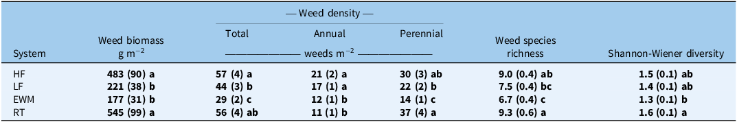
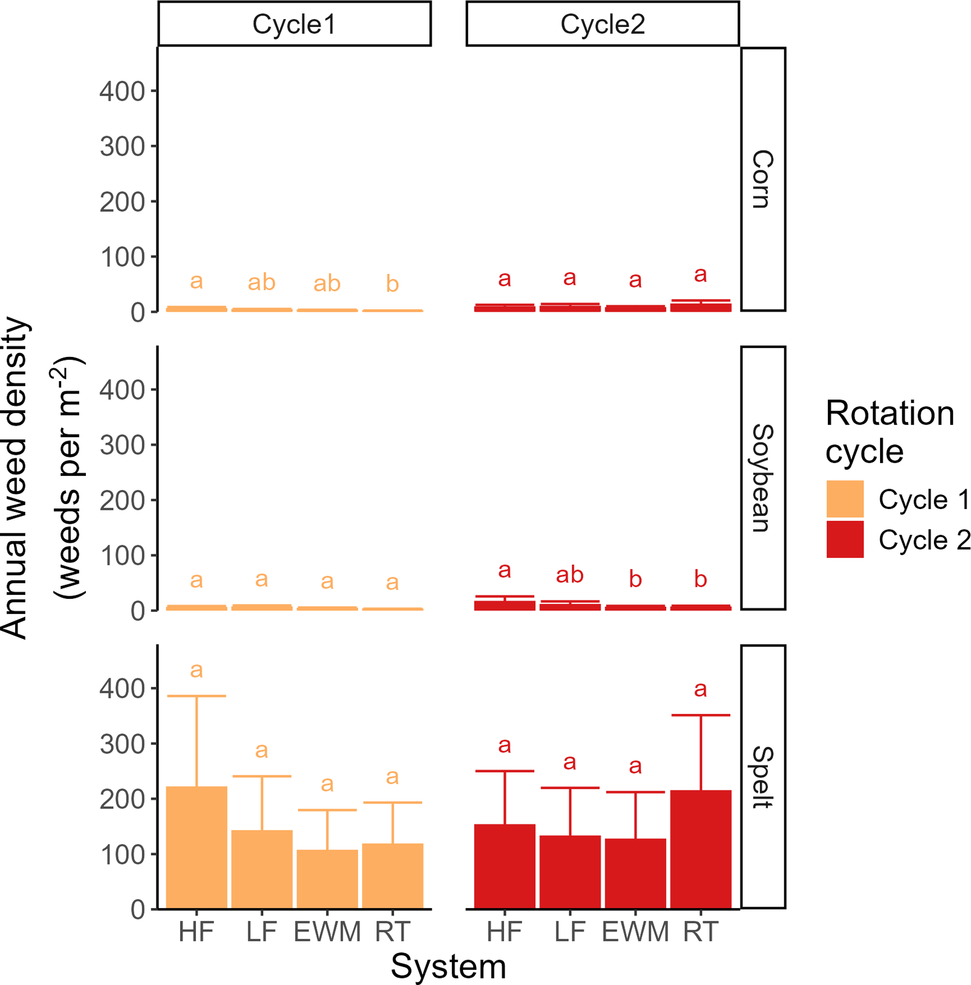
Effects of cropping system (HF, High Fertility; LF, Low Fertility; EWM, Enhanced Weed Management; or RT, Reduced Tillage) across all crops (corn, soybean, and spelt) and crop rotation cycles (first rotation cycle from 2005 to 2007 and second rotation cycle from 2008 to 2010) a .

In the first rotation cycle, total weed biomass in corn was greater for the HF system compared with the EWM system (Figure 2). Cropping system did not significantly affect total weed biomass in soybean or spelt. In the second rotation cycle, differences between systems were significant in both corn and soybean (Figure 2). In corn, total weed biomass was greatest for the RT system (back-transformed estimated mean ± SE: 1,075 ± 390 g m−2) and lowest for the EWM system (56 ± 23 g m−2). In soybean, total weed biomass was likewise greatest for the RT system (1,137 ± 411 g m−2) and lowest for the EWM system (195 ± 71 g m−2). Total weed biomass did not differ among systems in spelt.
Effects of cropping system within combinations of crop and rotation cycle on weed biomass. Data represent back-transformed estimated marginal means with 95% confidence intervals. Similar letters above bars indicate no significant difference (α = 0.05) within crops. HF, High Fertility; LF, Low Fertility; EWM, Enhanced Weed Management; RT, Reduced Tillage.

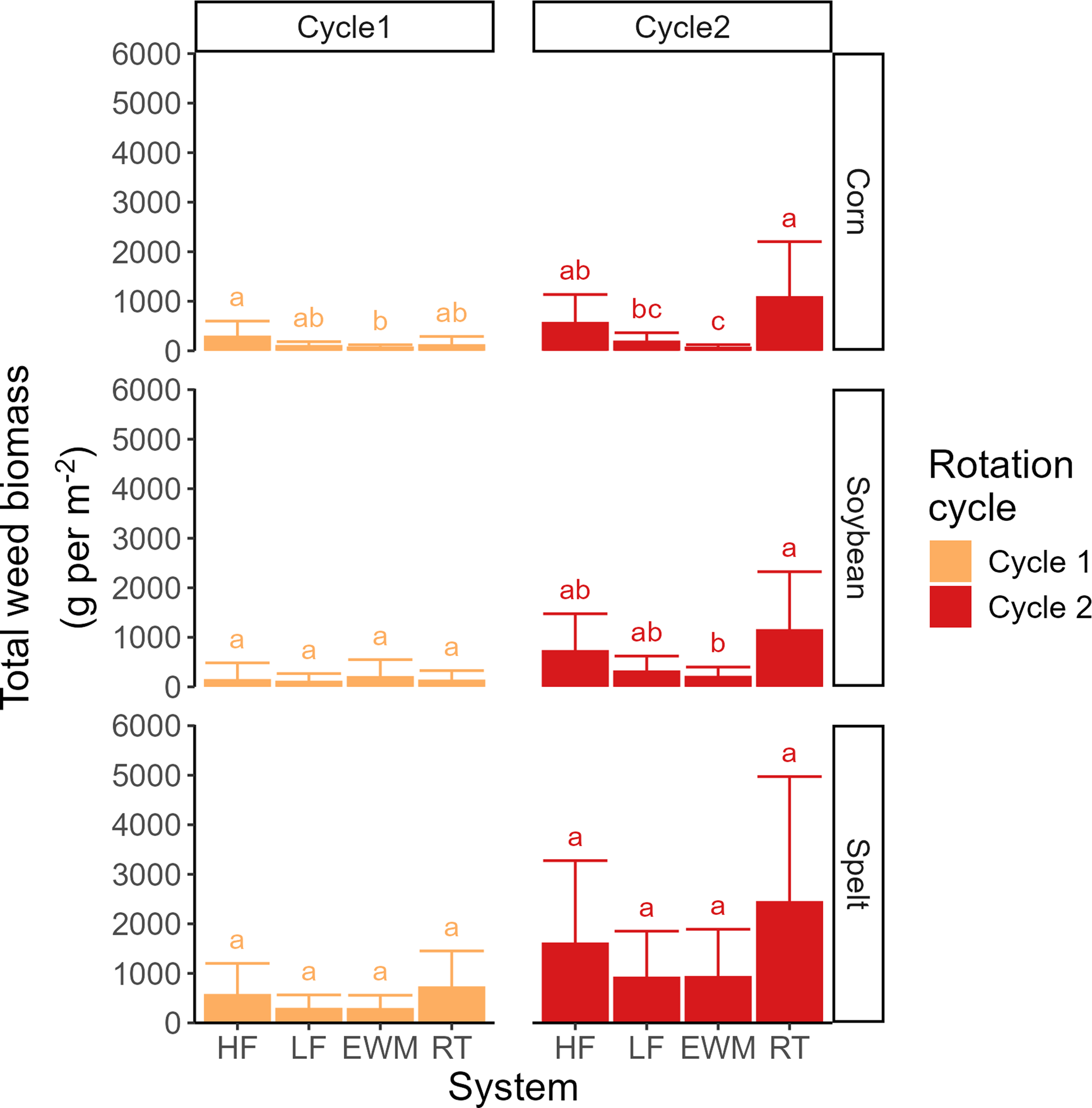
Total weed density showed a different trend in the first rotation cycle (Figure 3). In corn, total weed density was not different between systems. In soybean, total weed density was higher for the HF and LF systems than the EWM and RT systems. In spelt, total weed density was lowest for the EWM system (105 ± 18 weeds m−2). In the second rotation cycle, patterns in total weed density mirrored patterns in weed biomass, that is, greatest for the RT system and lowest for the EWM system in corn and soybean (Figure 3). In spelt, total weed density was not different between systems.
Effects of cropping system within combinations of crop and rotation cycle on total weed density. Data represent back-transformed estimated marginal means with 95% confidence intervals. Similar letters above bars indicate no significant difference (α = 0.05) within crops. HF, High Fertility; LF, Low Fertility; EWM, Enhanced Weed Management; RT, Reduced Tillage.

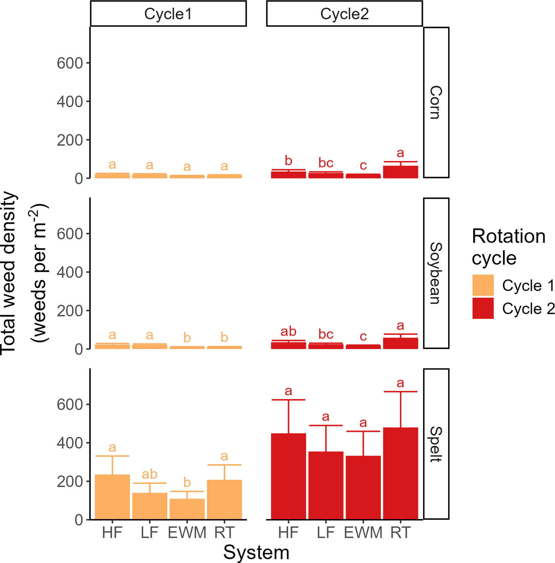
Annual weed density was affected by cropping system in two combinations of crop and rotation cycle (Figure 4). In corn in the first rotation cycle, annual weed density was greatest for the HF system (5 ± 1 weeds m−2) and lowest in the RT system (0.7 ± 0.4 weeds m−2). In soybean in the second rotation cycle, annual weed density was greatest for the HF system (15 ± 4 weeds m−2) and lowest for the EWM and RT systems (both 5 ± 1 weeds m−2). For the remaining combinations, no differences were found.
Effects of cropping system within combinations of crop and rotation cycle on annual weed density. Data represent back-transformed estimated marginal means with 95% confidence intervals. Similar letters above bars indicate no significant difference (α = 0.05) within crops. HF, High Fertility; LF, Low Fertility; EWM, Enhanced Weed Management; RT, Reduced Tillage.

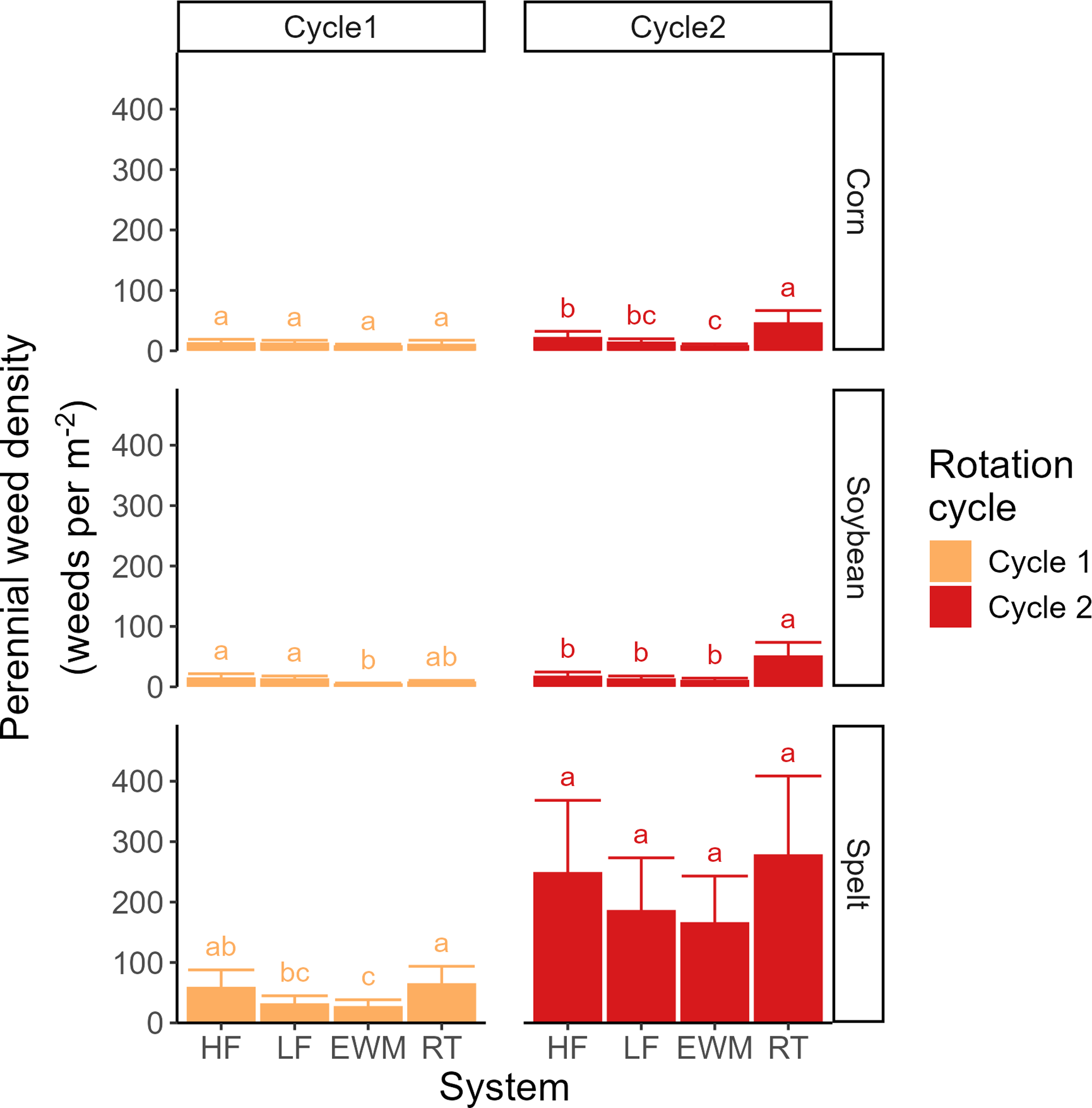
In contrast with annual weed density, perennial weed density largely mirrored total weed density (Figure 5). In the first rotation cycle, perennial weed density was lowest for the EWM system in soybean (3 ± 1 weeds m−2) and spelt (26 ± 5 weeds m−2). In the second rotation cycle, perennial weed density was greatest for the RT system in corn (45 ± 9 weeds m−2) and soybean (50 ± 10 weeds m−2). It was lowest for the EWM system in corn (7 ± 2 weeds m−2).
Effects of cropping system within combinations of crop and rotation cycle on perennial weed density. Data represent back-transformed estimated marginal means with 95% confidence intervals. Similar letters above bars indicate no significant difference (α = 0.05) within crops. HF, High Fertility; LF, Low Fertility; EWM, Enhanced Weed Management; RT, Reduced Tillage.

In the first rotation cycle, weed species richness in spelt was greater for the HF and RT systems (10.7 ± 1.3 and 11.2 ± 1.2 species, respectively) than the LF and EWM systems (both 5.5 ± 1.1 species; Figure 6). In the second rotation cycle, weed species richness in corn and soybean was greatest in the RT system (12.2 ± 0.8 and 11.6 ± 0.8 species, respectively). It was lowest for the EWM system in soybean (6.3 ± 0.8 species).
Effects of cropping system within combinations of crop and rotation cycle on weed species richness. Data represent back-transformed estimated marginal means with 95% confidence intervals. Similar letters above bars indicate no significant difference (α = 0.05) within crops. HF, High Fertility; LF, Low Fertility; EWM, Enhanced Weed Management; RT, Reduced Tillage.

Shannon-Wiener diversity only differed by system in spelt (Figure 7). For spelt in the first rotation cycle, Shannon-Wiener diversity was greatest for the RT system and lowest for the LF system. For spelt in the second rotation cycle, Shannon-Wiener diversity was greatest for the RT system and lowest for the HF system.
Effects of cropping system within combinations of crop and rotation cycle on Shannon-Wiener diversity. Data represent back-transformed estimated marginal means with 95% confidence intervals. Similar letters above bars indicate no significant difference (α = 0.05) within crops. HF, High Fertility; LF, Low Fertility; EWM, Enhanced Weed Management; RT, Reduced Tillage.

Effects of Crop on Weed Populations and Communities
The main effect of crop had significant effects on weed biomass; total, annual, and perennial weed density; and weed species richness (Table 1). The interaction between crop and rotation cycle influenced annual and perennial weed density, weed species richness, and Shannon-Wiener diversity (Table 1).
Main effects of crop largely reflected the fact that weed abundance was by far greatest in spelt (Table 3). Spelt weed biomass was greater than corn weed biomass for the EWM and RT systems in the first rotation cycle, plus the LF and EWM systems in the second rotation cycle. Spelt weed biomass was greater than soybean weed biomass for the RT system in the first rotation cycle and the EWM system in the second rotation cycle. Soybean weed biomass was greater than corn weed biomass for the EWM system in the second rotation cycle. Total weed biomass did not otherwise differ between crops within combinations of cropping system and rotation cycle.
Effects of crop (corn, soybean, or spelt) on weed biomass, density, and diversity within combinations of cropping system (HF, High Fertility; LF, Low Fertility; EWM, Enhanced Weed Management; or RT, Reduced Tillage) and crop rotation cycle (first rotation cycle from 2005 to 2007 or second rotation cycle from 2008 to 2010) a .

a Data represent back-transformed estimated marginal means with SEs. Means are the same as those shown in the figures and Table 4; pairwise comparisons are different. Different letters and bold type indicate significant differences (α = 0.05) among crops within system and rotation cycle.
Spelt had greater total weed density, annual weed density, and perennial weed density than corn and soybean for all eight combinations of crop and rotation cycle. Weed density generally did not differ between corn and soybean, except that annual weed density was greater in corn (13 ± 3 weeds m−2) than soybean (5 ± 1 weeds m−2) for the RT system in the second rotation cycle. In this case, annual weed density was still much greater in spelt (213 ± 54 weeds m−2).
The effect of crop on total weed biomass was less pronounced than the effect of crop on total weed density, because corn and soybean had fewer but larger weeds than spelt. Average weed size (calculated as the total biomass per square meter divided by the total density per square meter) was 18.0 ± 2.7 in corn, 18.7 ± 2.1 in soybean, and 4.4 ± 0.5 in spelt. These differences could reflect a combination of growing conditions (e.g., competitive effects) and species composition. Notably, there were many small individuals of species such as A. artemisiifolia in spelt. Because larger plants have greater competitive effects than smaller plants, weed biomass may be a better proxy for risk to crops than weed density.
In the first rotation cycle, weed species richness was greater in spelt than corn in the HF system and greater in spelt than corn and soybean in the RT system (Table 3). In the second rotation cycle, weed species richness was greater in spelt than corn and soybean in all systems (Table 3). However, Shannon-Wiener diversity generally did not differ among crops, with the exceptions of two cases in which Shannon-Wienerdiversity was greater in spelt than corn (first rotation cycle) and soybean was greater than spelt (second rotation cycle) (Table 3). We note that sampling areas differed by crop, that is, four 0.5-m2 sampling frames in corn and soybean and four 0.25-m2 sampling frames in spelt. If sampling areas had been the same among all crops, it is likely that measurements of weed diversity would have been greater in spelt relative to other crops. Consistency in sampling area is desirable for future studies of weed diversity.
Effects of Rotation Cycle on Weed Populations and Communities
The main effect of rotation cycle affected all measures of weed abundance and diversity (Table 1). These effects reflected an increase in weed abundance from the first rotation cycle (2005 to 2007) to the second rotation cycle (2008 to 2010) and a concomitant increase in weed diversity (Table 4). This increase was most pronounced for the RT system, that is, the system in which weeds were least well controlled. For the RT system in corn and soybean, all six measures of weed abundance and diversity increased from the first to the second rotation cycle. For the RT system in spelt, the same trend was observed for all measures, except annual weed density. Annual weed density did not differ between rotation cycles for any systems in spelt.
Effects of rotation cycle (first rotation cycle from 2005 to 2007 or second rotation cycle from 2008 to 2010) on weed biomass, density, and diversity within combinations of crop (corn, soybean, or spelt) and cropping system (HF, High Fertility; LF, Low Fertility; EWM, Enhanced Weed Management; or RT, Reduced Tillage) a .

a Data represent back-transformed estimated marginal means with SEs. Means are the same as those shown in figures and Table 3; pairwise comparisons are different. Different letters and bold type indicate significant differences (α = 0.05) among rotation cycles within crop and system.
For corn in the RT system, percentage change from Cycle 1 to Cycle 2 (calculation on raw data means) was 1,024% for weed biomass, 439% for total weed density, 1,050% for annual weed density, and 364% for perennial weed density. For soybean in the RT system, percentage change from Cycle 1 to Cycle 2 was 712% for weed biomass, 525% for total weed density, 262% for annual weed density, and 595% for perennial weed density. For spelt in the RT system, percentage change from Cycle 1 to Cycle 2 was 214% for weed biomass, 111% for total weed density, 14% for annual weed density, and 347% for perennial weed density. These findings suggest that perennial weeds played a major role in driving increased weed density in the RT system.
Differences between rotation cycles were less pronounced for the HF, LF, and EWM systems in corn and soybean. However, we observed some cases in which weed abundance and diversity were greater in the second rotation cycle: total weed density for the HF system in corn; annual weed density and Shannon-Wiener diversity for the LF and EWM systems in corn; weed biomass and annual weed density for the HF system in soybean; and total weed density and perennial weed density for the EWM system in soybean. These findings suggest that weed abundance and diversity increased across the experiment, although these trends were strongest for the RT system. Future research should test how weed communities might be similar or different during the transition to alternative RT systems in both organic and conventional production.
Management Implications
Weed biomass and density were generally greater in the HF and RT systems than in the LF and EWM systems (Table 2). This finding supports the interpretation that weed species were able to capitalize on increased soil fertility and reduced disturbance in the HF and RT systems, respectively. High weed abundance in the HF system occurred despite high crop yields in this system. Caldwell et al. (Reference Caldwell, Mohler, Ketterings and DiTommaso2014) provided a detailed analysis of crop yield in this experiment. Briefly, corn and soybean yields were largely similar between HF, LF, and EWM systems. System-by-year means in these systems ranged from 5.2 to 10.8 Mg ha−1 in corn and 2.0 to 3.2 Mg ha−1 in soybean (Caldwell et al. Reference Caldwell, Mohler, Ketterings and DiTommaso2014). Corn and soybean yields were lower in the RT system, which suffered from equipment difficulties, especially early in the experiment. Spelt yield was greatest in the HF and EWM systems during the transitional period (up to 3.5 Mg ha−1) and variable after the transitional period (Caldwell et al. Reference Caldwell, Mohler, Ketterings and DiTommaso2014).
One might expect that relatively high crop yields in the HF system would indicate good crop competitiveness and therefore weed suppression. We do not discount the possibility that crop–weed competition contributed to weed suppression. However, the co-occurrence of high crop yields with high weed abundance in the HF system suggests that enhanced soil fertility likely had significant direct effects on weeds. Many agricultural weeds are highly responsive to fertilization, which can promote their germination, emergence, growth, and reproduction (Little et al. Reference Little, DiTommaso, Westbrook, Ketterings and Mohler2021; Zimdahl Reference Zimdahl2018). Thus, positive effects of soil fertility on weeds may have outweighed negative effects of crop competition against the weeds, leading to high weed abundance in the HF system. It is also possible that higher compost application rates in the HF system led to more weed seed introductions (Kulesza et al. Reference Kulesza, Leon, Sosinski, Kilroy, Meis, Castillo and Wilson2024). On the other hand, the HF system (like the EWM system) included an overwintering cover crop after corn, which may have reduced the potential for weed expansion and helped minimize differences between the HF and LF systems within combinations of crop and rotation cycle.
In the EWM system, soil disturbance frequency and intensity were increased through additional tillage and cultivation operations. In addition, spelt was seeded at a higher rate to enhance crop–weed interference. Perennial weed density was sometimes lower in the EWM system than in the LF system, suggesting that increased soil disturbance helped increase weed control. Conversely, decreased soil disturbance (RT vs. LF) caused a notable increase in perennial weed density in the second rotation cycle. These perennial weeds included species such as C. arvense and S. arvensis. Reducing soil disturbance in organic arable crops is desirable from soil quality and environmental health perspectives, but often challenging due largely to problems with perennial weed control (Krauss et al. Reference Krauss, Berner, Perrochet, Frei, Niggli and Mäder2020; Mäder and Berner Reference Mäder and Berner2012). Weed control is a primary barrier to the development of reduced-tillage organic systems. Perennial weeds are particularly difficult to control in these systems (Armengot et al. Reference Armengot, Berner, Blanco-Moreno, Mäder and Sans2015). In our experiment, the RT system experienced a weed community shift to perennials that contributed to crop yield declines. This finding is consistent with the reduced disturbance in this system, although it may have also reflected issues encountered in early years (i.e., planter units did not track scraped rows).
Increases in weed abundance are a common occurrence during the transition to organic grain production, because weed species already present in a field may be more likely to survive, set seed, and contribute to the soil seedbank when synthetic herbicides are eliminated. To bring weeds under control, it is helpful to grow more competitive crops that can be cultivated aggressively during the transitional period (Mohler et al. Reference Mohler, Teasdale and DiTommaso2021). Consistent with this recommendation, we found that spelt had greater total weed biomass and density than soybean or corn. Differences in crop life cycles and row spacing (spelt is a winter annual seeded in 19-cm rows, whereas soybean and corn are summer annuals seeded in 76-cm rows) may have contributed to this trend. It is likely that soybean and corn greatly benefited from interrow cultivation, which did not occur in the fall-planted spelt. Cultivation events in this experiment provided 73% weed control in soybean and up to 91% weed control in corn (Mohler et al. Reference Mohler, Marschner, Caldwell and DiTommaso2016).
Increased weed diversity associated with healthy crop rotations has been linked with ecological and potentially agronomic benefits (Adeux et al. Reference Adeux, Vieren, Carlesi, Bàrberi, Munier-Jolain and Cordeau2019; MacLaren et al. Reference MacLaren, Storkey, Menegat, Metcalfe and Dehnen-Schmutz2020; Storkey and Neve Reference Storkey and Neve2018). Agronomic benefits could reflect an association between increased weed community evenness (a component of biodiversity) and reduced weed competitiveness and biomass (Adeux et al. Reference Adeux, Vieren, Carlesi, Bàrberi, Munier-Jolain and Cordeau2019; Storkey and Neve Reference Storkey and Neve2018). In this study, we observed an increase in weed diversity from the first to the second rotation cycle in all systems, associated with the transition to organic management. This finding is consistent with previous research (Ryan et al. Reference Ryan, Smith, Mirsky, Mortensen and Seidel2010) and could reflect a weakening of strong weed community assembly filters and a diversification of resource pools.
Overall, the results of this experiment illustrate how different cropping systems affect weed populations and communities during the transition to certified organic grain production and the post-transition period. Although this systems-level experiment did not distinguish the roles of individual management practices in driving these effects, it does demonstrate how complete management programs (defined in terms of soil disturbance, cover crops, and fertility) are associated with different levels of weed biomass, density, and diversity. Our results suggest the importance of management practices that increase the competitiveness of crops relative to weeds, such as the elevated seeding rates implemented for spelt in the EWM system. Combined with judicious use of soil disturbance, these practices can help minimize weed challenges for grain farmers choosing to transition their farms to certified organic enterprises.
Supplementary material
To view supplementary material for this article, please visit https://doi.org/10.1017/wsc.2026.10093
Acknowledgments
The authors are grateful to the staff, faculty, students, Cornell Statistical Consulting Unit personnel, and organic farmer advisors who invested their knowledge, skills, and time into the Cornell Organic Cropping Systems experiment. We recognize Charles L. Mohler for his role in the conception, design, and implementation of the experiment and dedicate this article to his memory.
Funding statement
This work was supported by the USDA National Institute for Food and Agriculture Organic Agriculture Research and Extension Initiative (Project numbers 2004-51300-02230, 2009-51300-05586, and 2020-51300-32183).
Competing interests
The authors declare no conflicts of interest.


 Open access