


1. Introduction
Aedes albopictus and Aedes aegypti mosquitoes are the primary vectors of mosquito-borne diseases such as dengue, Zika, yellow fever and chikungunya, causing considerable morbidity and mortality globally each year [Reference Naddaf21, 29]. In recent years, increasing attention has been focused on utilising sustainable biotechnological approaches for mosquito control. Biological control strategies, such as the sterile insect technique (SIT) and the incompatible insect technique (IIT), aim to suppress field mosquito populations. SIT involves releasing sterile male mosquitoes produced through radiation [Reference Lees, Gilles and Hendrichs10], while IIT relies on releasing Wolbachia-infected males [Reference Bourtzis, Dobson and Xi2, Reference Dodson, Pujhari and Brustolin6]. Both techniques have been extensively studied and tested. Additionally, their combination has been explored as an integrated approach [Reference Kittayapong, Ninphanomchai and Limohpasmanee8, Reference Zheng, Zhang and Li38]. The effectiveness of these biotechnological interventions is well documented.
Mathematical modelling plays a crucial role in understanding the evolutionary mechanisms of mosquito populations, analysing key factors influencing the spread of mosquito-borne diseases and aiding the development of rational control strategies of mosquitoes. In particular, mathematical models for the SIT have provided long-term theoretical support for studying the dynamics of interactions between wild and sterile mosquitoes [Reference Cai, Ai and Li4, Reference Yu and Li32], which is essential for the practical implementation of SIT. The emergence of modelling analyses for the IIT has significantly advanced the development of biological control technologies for mosquitoes [Reference Li and Zhao11, Reference Wan, Wu, Fan and Li26, Reference Yu31, Reference Zheng, Tang, Yu and Qiu35]. In recent years, the combination of SIT and IIT has attracted growing attention from biomathematicians, leading to the development of relevant models [Reference Zheng, Yu and Li37, Reference Zheng, Zhang and Li38], which offer valuable insights into designing integrated control measures of mosquitoes and optimising release strategies. In this study, we collectively refer to released Wolbachia-infected mosquitoes and radiation-induced sterile mosquitoes as sterile mosquitoes. Notably, we highlight a time-switching ordinary differential equation model introduced in [Reference Yu and Li33], which describes the release of sterile mosquitoes to suppress wild mosquito populations. This model explicitly considers the sexual lifespan of sterile mosquitoes, during which they are active. It is formulated as follows
 \begin{align} {\begin{cases}\begin{aligned} &\frac {\text{d}w}{\text{d}t} = w \left [\frac {aw}{w+c} - \gamma - \delta (w+c)\right ]\!, & t &\in (nT, nT+\overline {T}], \\[8pt] &\frac {\text{d}w}{\text{d}t} = w (a - \gamma - \delta w), & t &\in (nT+\overline {T}, (n+1)T], \end{aligned}\end{cases}} \end{align}
where
 $w$
represents the number of wild mosquitoes at time
$w$
represents the number of wild mosquitoes at time
 $t$
. The parameters
$t$
. The parameters
 $a$
,
$a$
,
 $\gamma$
and
$\gamma$
and
 $\delta$
denote the birth rate, natural death rate and density-dependent mortality coefficient of wild mosquitoes, respectively. It is naturally assumed that
$\delta$
denote the birth rate, natural death rate and density-dependent mortality coefficient of wild mosquitoes, respectively. It is naturally assumed that
 $a \gt \gamma$
. The parameters
$a \gt \gamma$
. The parameters
 $c$
,
$c$
,
 $T$
and
$T$
and
 $\overline {T}$
represent the release amount, release period and sexual lifespan of sterile mosquitoes, respectively, with the condition
$\overline {T}$
represent the release amount, release period and sexual lifespan of sterile mosquitoes, respectively, with the condition
 $T \gt \overline {T}$
. Sterile mosquitoes are introduced impulsively and periodically at discrete time points
$T \gt \overline {T}$
. Sterile mosquitoes are introduced impulsively and periodically at discrete time points
 $T_n = nT$
, where
$T_n = nT$
, where
 $n = 0,1,2,\dots$
. Two key thresholds,
$n = 0,1,2,\dots$
. Two key thresholds,
 $ c^{*}$
and
$ c^{*}$
and
 $T^{*}$
, are defined to characterise the dynamics of (1.1), see Theorem 2.2–2.4 in [Reference Yu and Li33]. The model provides concise analytical results and theoretically derived release strategies capable of eliminating wild mosquito populations. The biological relevance of (1.1) is well founded, and conclusions on it closely align with real-world observations, making it a widely studied framework [Reference Pan, Shu and Wang23, Reference Wang, Chen, Zheng and Yu28, Reference Yan, Guo and Yu30, Reference Zheng and Yu36].
$T^{*}$
, are defined to characterise the dynamics of (1.1), see Theorem 2.2–2.4 in [Reference Yu and Li33]. The model provides concise analytical results and theoretically derived release strategies capable of eliminating wild mosquito populations. The biological relevance of (1.1) is well founded, and conclusions on it closely align with real-world observations, making it a widely studied framework [Reference Pan, Shu and Wang23, Reference Wang, Chen, Zheng and Yu28, Reference Yan, Guo and Yu30, Reference Zheng and Yu36].
The competition between Ae. albopictus and Ae. aegypti mosquitoes cannot be overlooked when employing sterile mosquitoes to suppress the Ae. albopictus population. Studies have shown that both Aedes species are rapidly invading nearly all continents, with extensive overlapping distributions observed primarily in the southern United States, eastern Brazil, large regions of Southeast Asia and southern China. Moreover, projections indicate that these overlapping areas will persist in the coming years [Reference Laporta, Potter and Oliveira9, Reference Nie and Feng22].
Furthermore, Ae. albopictus and Ae. aegypti mosquitoes share similar ecological niches and exhibit no reproductive isolation, leading to various forms of competitive interactions [Reference Ali, Tayeb and Vauchelet3, Reference Liu, Tian and Ruan14, Reference Tian and Ruan25, Reference Zhou, Liu and Liu39]. To incorporate interspecific competition into the modelling framework, we extend system (1.1) by introducing the dynamics of a competing mosquito population, resulting in the following time-switching ordinary differential system

where
 $U$
and
$U$
and
 $V$
denote the population sizes of Ae. albopictus and Ae. aegypti at time
$V$
denote the population sizes of Ae. albopictus and Ae. aegypti at time
 $t$
, respectively. All parameters are positive, where
$t$
, respectively. All parameters are positive, where
 $a_{i}$
and
$a_{i}$
and
 $\gamma _{i}$
represent the birth and death rates, while
$\gamma _{i}$
represent the birth and death rates, while
 $\delta _{i}$
and
$\delta _{i}$
and
 $\xi _{i}$
are the intraspecific or interspecific competition coefficients for
$\xi _{i}$
are the intraspecific or interspecific competition coefficients for
 $U$
and
$U$
and
 $V$
(
$V$
(
 $i=1,2$
), respectively. We assume
$i=1,2$
), respectively. We assume
 $a_{i} \gt \gamma _{i}$
for biological relevance. Additionally, the parameters
$a_{i} \gt \gamma _{i}$
for biological relevance. Additionally, the parameters
 $c$
,
$c$
,
 $T$
and
$T$
and
 $\overline {T}$
represent the release quantity, release period and sexual lifespan of the Ae. albopictus-type sterile mosquitoes, respectively, with the condition
$\overline {T}$
represent the release quantity, release period and sexual lifespan of the Ae. albopictus-type sterile mosquitoes, respectively, with the condition
 $T \gt \overline {T}$
.
$T \gt \overline {T}$
.
Mosquito reproduction and propagation are environmentally dependent, and so consideration of factors such as wind speed and spatial heterogeneity can inject necessary realism into theoretical studies on model. It is well known that reaction-diffusion equations are powerful tools for describing the spatial and temporal evolution of populations [Reference Almeida, Bliman, Nguyen and Vauchelet1, Reference Cantrell and Cosner5]. In general, strong winds force mosquitoes to change their flight paths, severely affecting their daily activities. The two types of mosquitoes have different expansion capabilities [Reference Nie and Feng22] and suffer from strong winds in different levels. This can be depicted by assigning different diffusion and advection rates to the two Aedes species in the formation of the reaction-diffusion system. In addition, the size of the area and boundary conditions can significantly influence the evolution of the population and thus the design of release strategies. To capture these features, we consider the following two species competing reaction-diffusion-advection switching system

where
 $U(t,x)$
and
$U(t,x)$
and
 $V(t,x)$
are the densities of
$V(t,x)$
are the densities of
 $\textit {Ae. albopictus}$
and
$\textit {Ae. albopictus}$
and
 $\textit {Ae. aegypti}$
mosquitoes at time
$\textit {Ae. aegypti}$
mosquitoes at time
 $t$
and location
$t$
and location
 $x$
, respectively.
$x$
, respectively.
 $L\gt 0$
is the length of the domain under consideration.
$L\gt 0$
is the length of the domain under consideration.
 $d_{i}\gt 0,i=1,2$
are the diffusion rates of
$d_{i}\gt 0,i=1,2$
are the diffusion rates of
 $U$
and
$U$
and
 $V$
, respectively. The other parameters
$V$
, respectively. The other parameters
 $\alpha ,\beta ,b\geq 0$
, where
$\alpha ,\beta ,b\geq 0$
, where
 $\alpha$
and
$\alpha$
and
 $\beta$
are the advection coefficients of
$\beta$
are the advection coefficients of
 $U$
and
$U$
and
 $V$
, respectively, and
$V$
, respectively, and
 $b$
denotes the loss rate of both species at the downstream end
$b$
denotes the loss rate of both species at the downstream end
 $x=L$
. It is noted that if
$x=L$
. It is noted that if
 $b=0$
, no individual can pass through the boundary, and we refer to this as a no-flux boundary [Reference Lou and Lutscher15], as shown in the upstream point
$b=0$
, no individual can pass through the boundary, and we refer to this as a no-flux boundary [Reference Lou and Lutscher15], as shown in the upstream point
 $x=0$
of (1.3). In a biological sense, this can be explained as a high wall or cliff blocking the mosquito’s path. While if
$x=0$
of (1.3). In a biological sense, this can be explained as a high wall or cliff blocking the mosquito’s path. While if
 $b\gt 0$
, individuals can diffuse outward and cause loss after reaching the boundary, in which case the environment is open. For more research on open- or closed-advective environments, we refer to [Reference Lou, Nie and Wang16, Reference Lou, Xiao and Zhou17, Reference Lou, Zhao and Zhou19, Reference Meng, Lin and Pedersen20, Reference Tang and Chen24, Reference Wang, Wang and Zhao27] and references therein.
$b\gt 0$
, individuals can diffuse outward and cause loss after reaching the boundary, in which case the environment is open. For more research on open- or closed-advective environments, we refer to [Reference Lou, Nie and Wang16, Reference Lou, Xiao and Zhou17, Reference Lou, Zhao and Zhou19, Reference Meng, Lin and Pedersen20, Reference Tang and Chen24, Reference Wang, Wang and Zhao27] and references therein.
System (1.3) makes sense, and its investigation has practical applications. In view of the high cost of sterile mosquitoes, finding the minimal release amount and the maximal release period that can eliminate both Aedes mosquitoes becomes a key objective in the development of an economic release strategy. This can be reached by obtaining conditions on the global asymptotic stability of the trivial steady state of system (1.3) with parameters
 $c$
and
$c$
and
 $T$
. Though there is limited amount of work on time-switching single reaction-diffusion equations [Reference Liu, Yu, Chen and Guo13], fewer studies are available on switching systems. This makes (1.3) of research interest.
$T$
. Though there is limited amount of work on time-switching single reaction-diffusion equations [Reference Liu, Yu, Chen and Guo13], fewer studies are available on switching systems. This makes (1.3) of research interest.
In order to implement the comparison principle, we let
 $U=e^{\frac {\alpha }{d_{1}}x}u$
and
$U=e^{\frac {\alpha }{d_{1}}x}u$
and
 $V=e^{\frac {\beta }{d_{2}}x}v$
. Then, (1.3) is transformed into
$V=e^{\frac {\beta }{d_{2}}x}v$
. Then, (1.3) is transformed into

Assume further that the initial values
 $(u_{0},v_{0})$
satisfies
$(u_{0},v_{0})$
satisfies
 $u_{0},v_{0}\in C([0,L])$
. Then it is easy to see that the solution to (1.4) exists uniquely and is uniformly bounded on the interval
$u_{0},v_{0}\in C([0,L])$
. Then it is easy to see that the solution to (1.4) exists uniquely and is uniformly bounded on the interval
 $(0,\overline {T}],(\overline {T},T],(T,T+\overline {T}],\cdots$
, and thus the well-posedness of (1.4) is established. In this paper, we mainly discuss the periodic dynamics of system (1.4) and find the optimal release amount
$(0,\overline {T}],(\overline {T},T],(T,T+\overline {T}],\cdots$
, and thus the well-posedness of (1.4) is established. In this paper, we mainly discuss the periodic dynamics of system (1.4) and find the optimal release amount
 $c$
and release period
$c$
and release period
 $T$
that can eliminate both Aedes mosquitoes.
$T$
that can eliminate both Aedes mosquitoes.
The rest of the paper is organised as follows. In Section 2, we discuss the eigenvalue problem for the corresponding single-species equations and define two thresholds of the release period, which are crucial for the analysis of system (1.4). In Section 3, two further thresholds for the release period are defined, generated by the eigenvalue problem of the linearised equations of (1.4) at the two semi-trivial periodic solutions, respectively. Then some dynamics of system (1.4) are given. Numerical examples are provided in Section 4 to confirm our theoretical results. A brief conclusion is given in Section 5.
2. Dynamics of single-species equations
This section investigates the dynamics of the corresponding single-species problems, primarily through the eigenvalue method, to establish several key thresholds. These findings facilitate the subsequent analysis of the semi-trivial periodic solutions in system (1.4).
For the
 $\textit {Ae. albopictus}$
population
$\textit {Ae. albopictus}$
population
 $u$
, we have
$u$
, we have
 \begin{equation} {\left \{\begin{aligned} &u_{t}=d_{1}u_{xx}+\alpha u_{x}+u\left [\frac {a_{1}e^{\frac {\alpha }{d_{1}}x}u}{e^{\frac {\alpha }{d_{1}}x}u+c}-\gamma _{1}-\delta _{1}\left (e^ {\frac {\alpha }{d_{1}}x}u+c\right )\right ]\!,&t&\in (nT,nT+\overline {T}],\,x\in (0,L),\\[6pt] &u_{t}=d_{1}u_{xx}+\alpha u_{x}+u\left (a_{1}-\gamma _{1}-\delta _{1}e^{\frac {\alpha }{d_{1}}x}u\right )\!,&t&\in (nT+\overline {T},(n+1)T],\,x\in (0,L),\\[3pt] &u_{x}(t,0)=0,&t&\gt 0,\\[3pt] &d_{1}u_{x}(t,L)=-b\alpha u(t,L),&t&\gt 0,\\[3pt] &u(0,x)=e^{-\frac {\alpha }{d_{1}}x}U_{0}(x)=u_{0}(x)\geq ,\not \equiv 0,&x&\in [0,L], \end{aligned}\right .} \end{equation}
and its eigenvalue problem linearised at
 $u=0$
$u=0$
 \begin{equation} {\left \{\begin{aligned} &\phi _{t}=d_{1}\phi _{xx}+\alpha \phi _{x}-(\gamma _{1}+\delta _{1}c)\phi +\mu \phi ,\,&t&\in (0,\overline {T}],\,x\in (0,L),\\[3pt] &\phi _{t}=d_{1}\phi _{xx}+\alpha \phi _{x}+(a_{1}-\gamma _{1})\phi +\mu \phi ,\,&t&\in (\overline {T},T],\,x\in (0,L),\\[3pt] &\phi _{x}(t,0)=0,\,&t&\in [0,T],\\[3pt] &d_{1}\phi _{x}(t,L)=-b\alpha \phi (t,L),\,&t&\in [0,T],\\[3pt] &\phi (0,x)=\phi (T,x),\,&x&\in [0,L]. \end{aligned}\right .} \end{equation}
Before discussing problem (2.2), we start with a reasonable assumption that population
 $u$
can persist in the case of no sterile mosquitoes being released, namely,
$u$
can persist in the case of no sterile mosquitoes being released, namely,
 $c=0$
. Then, (2.1) reduces to the following problem
$c=0$
. Then, (2.1) reduces to the following problem
 \begin{equation} {\left \{\begin{aligned} &u_{t}=d_{1}u_{xx}+\alpha u_{x}+u\left (a_{1}-\gamma _{1}-\delta _{1}e^ {\frac {\alpha }{d_{1}}x}u\right )\!,\,&t&\gt 0,\,x\in (0,L),\\ &u_{x}(t,0)=0,\,&t&\gt 0,\\[3pt] &d_{1}u_{x}(t,L)=-b\alpha u(t,L),\,&t&\gt 0,\\[3pt] &u(0,x)=u_{0}(x)\geq ,\not \equiv 0,\,&x&\in [0,L], \end{aligned}\right .} \end{equation}
and its corresponding eigenvalue problem
 \begin{equation} {\left \{\begin{aligned} &d_{1}\varphi _{xx}+\alpha \varphi _{x}+(a_{1}-\gamma _{1})\varphi +\lambda \varphi =0,\,x\in (0,L),\\[3pt] &\varphi _{x}(0)=0,\,d_{1}\varphi _{x}(L)=-b\alpha \varphi (L). \end{aligned}\right .} \end{equation}
According to [Reference Lou and Zhou18], the principal eigenvalue of (2.4), we denote as
 $\lambda _{\alpha ,1}$
, is given by
$\lambda _{\alpha ,1}$
, is given by
 \begin{equation*}\lambda _{\alpha ,1}=\inf _{0\neq \varphi \in W^{1,2}}\frac {b\alpha e^{\frac {\alpha }{d_{1}}L}\varphi ^{2}(L)+d_{1}\int _{0}^{L}e^{\frac {\alpha }{d_{1}}x}\varphi _{x}^{2}\text{d}x-(a_{1} -\gamma _{1})\int _{0}^{L}e^{\frac {\alpha }{d_{1}}x}\varphi ^{2}\text{d}x}{\int _{0}^{L}e^{\frac {\alpha }{d_{1}}x}\varphi ^{2}\text{d}x}\,\,\textrm {for}\,b\in [0,+\infty ),\end{equation*}
and
 \begin{equation*}\lambda _{\alpha ,1}=\inf _{\varphi \in W^{1,2},\varphi _{x}(0)=\varphi (L)=0}\frac{\text{d}_{1}\int _{0}^{L}e^{\frac {\alpha }{d_{1}}x}\varphi _{x}^{2}\text{d}x-(a_{1} -\gamma _{1})\int _{0}^{L}e^{\frac {\alpha }{d_{1}}x}\varphi ^{2}\text{d}x}{\int _{0}^{L}e^{\frac {\alpha }{d_{1}}x}\varphi ^{2}\text{d}x}\,\,\textrm {for}\,b=+\infty .\end{equation*}
It is easy to find that
 $\lambda _{\alpha ,1}\geq -(a_{1} -\gamma _{1})$
, and by the assumption that
$\lambda _{\alpha ,1}\geq -(a_{1} -\gamma _{1})$
, and by the assumption that
 $\lambda _{\alpha ,1}\lt 0$
.
$\lambda _{\alpha ,1}\lt 0$
.
Now returning to (2.2), we give a critical value of the parameter
 $T$
to determine the sign of the principal eigenvalue
$T$
to determine the sign of the principal eigenvalue
 $\mu _{1}$
of (2.2), which brings insights into the dynamics analysis of (2.1).
$\mu _{1}$
of (2.2), which brings insights into the dynamics analysis of (2.1).
Lemma 2.1. There exists a unique
 \begin{equation*}T^{*}\,:\!=\,-\frac {(a_{1}+\delta _{1}c)\overline {T}}{\lambda _{\alpha ,1}}\gt 0\end{equation*}
such that
 $\mu _{1}=0$
if
$\mu _{1}=0$
if
 $T=T^{*}$
,
$T=T^{*}$
,
 $\mu _{1}\lt 0$
if
$\mu _{1}\lt 0$
if
 $T\gt T^{*}$
and
$T\gt T^{*}$
and
 $\mu _{1}\gt 0$
if
$\mu _{1}\gt 0$
if
 $T\lt T^{*}$
.
$T\lt T^{*}$
.
Proof. Let
 $\phi (t,x)=f(t)\varphi (x)$
, where
$\phi (t,x)=f(t)\varphi (x)$
, where
 $\varphi (x)$
is the eigenfunction corresponding to the eigenvalue
$\varphi (x)$
is the eigenfunction corresponding to the eigenvalue
 $\lambda _{\alpha ,1}$
of (2.4), and
$\lambda _{\alpha ,1}$
of (2.4), and
 $f(t)$
is a continuous function and satisfies
$f(t)$
is a continuous function and satisfies
 $f(t)\gt 0$
for
$f(t)\gt 0$
for
 $t\gt 0$
. Substituting it into problem (2.2) yields
$t\gt 0$
. Substituting it into problem (2.2) yields
 \begin{equation} {\left \{\begin{aligned} &f_{t}\varphi =d_{1}f\varphi _{xx}+\alpha f\varphi _{x}-(\gamma _{1}+\delta _{1}c)f\varphi +\mu _{1}f\varphi ,\,&t&\in (0,\overline {T}],\,x\in (0,L),\\[3pt] &f_{t}\varphi =d_{1}f\varphi _{xx}+\alpha f\varphi _{x}+(a_{1}-\gamma _{1})f\varphi +\mu _{1}f\varphi ,\,&t&\in (\overline {T},T],\,x\in (0,L),\\[3pt] &f(0)=f(T). \end{aligned}\right .} \end{equation}
Divide both sides of the first two equations by
 $f\varphi$
and use (2.4) to obtain
$f\varphi$
and use (2.4) to obtain
 \begin{equation} {\left \{\begin{aligned} &\frac {f_{t}}{f}=-\lambda _{\alpha ,1}-(a_{1}+\delta _{1}c)+\mu _{1},\,&t&\in (0,\overline {T}],\\[3pt] &\frac {f_{t}}{f}=-\lambda _{\alpha ,1}+\mu _{1},\,&t&\in (\overline {T},T],\\[3pt] &f(0)=f(T). \end{aligned}\right .} \end{equation}
Integrating the first and second equations of (2.6) from 0 to
 $\overline {T}$
and
$\overline {T}$
and
 $\overline {T}$
to
$\overline {T}$
to
 $T$
, respectively, produces
$T$
, respectively, produces
 \begin{equation*}\ln {f(\overline {T})}-\ln {f(0)}=[\!-\lambda _{\alpha ,1}-(a_{1}+\delta _{1}c)+\mu _{1}]\overline {T}\end{equation*}
and
 \begin{equation*}\ln {f(T)}-\ln {f(\overline {T})}=(\!-\lambda _{\alpha ,1}+\mu _{1})T-(\!-\lambda _{\alpha ,1}+\mu _{1})\overline {T}.\end{equation*}
Adding the above two equations results in
 $\mu _{1}=\lambda _{\alpha ,1}+\frac {(a_{1}+\delta _{1}c)\overline {T}}{T}$
. It is clear that
$\mu _{1}=\lambda _{\alpha ,1}+\frac {(a_{1}+\delta _{1}c)\overline {T}}{T}$
. It is clear that
 $\mu _{1}$
is strictly decreasing with respect to
$\mu _{1}$
is strictly decreasing with respect to
 $T$
. Also, noting that
$T$
. Also, noting that
 $-(a_{1} -\gamma _{1})\leq \lambda _{\alpha ,1}\lt 0$
, we have
$-(a_{1} -\gamma _{1})\leq \lambda _{\alpha ,1}\lt 0$
, we have
 $\mu _{1}\rightarrow \lambda _{\alpha ,1}+(a_{1}+\delta _{1}c)\gt 0$
as
$\mu _{1}\rightarrow \lambda _{\alpha ,1}+(a_{1}+\delta _{1}c)\gt 0$
as
 $T\rightarrow \overline {T}^{+}$
and
$T\rightarrow \overline {T}^{+}$
and
 $\mu _{1}\rightarrow \lambda _{\alpha ,1}\lt 0$
as
$\mu _{1}\rightarrow \lambda _{\alpha ,1}\lt 0$
as
 $T\rightarrow +\infty$
. The desired result follows immediately from the intermediate value theorem and the monotonicity of
$T\rightarrow +\infty$
. The desired result follows immediately from the intermediate value theorem and the monotonicity of
 $\mu _{1}$
.
$\mu _{1}$
.
Based on the above analysis, we establish the following results on the dynamics of (2.1).
Theorem 2.1.
Assume that
 $c\geq \frac {a_{1}}{\delta _{1}}$
. If
$c\geq \frac {a_{1}}{\delta _{1}}$
. If
 $T\leq T^{*}$
, then the steady state
$T\leq T^{*}$
, then the steady state
 $0$
of (2.1) is globally asymptotically stable. If
$0$
of (2.1) is globally asymptotically stable. If
 $T\gt T^{*}$
, then (2.1) has a unique globally asymptotically stable positive T-periodic solution
$T\gt T^{*}$
, then (2.1) has a unique globally asymptotically stable positive T-periodic solution
 $u^{*}(t,x)$
.
$u^{*}(t,x)$
.
Proof. First, we assume that
 $T\leq T^{*}$
.
$T\leq T^{*}$
.
If
 $T\lt T^{*}$
, define
$T\lt T^{*}$
, define
 $\overline {u}=Me^{-\mu _{1}t}\phi (t,x)$
, where
$\overline {u}=Me^{-\mu _{1}t}\phi (t,x)$
, where
 $M\gt 0$
is large enough such that
$M\gt 0$
is large enough such that
 $\overline {u}(0,x)\geq u(0,x)$
,
$\overline {u}(0,x)\geq u(0,x)$
,
 $x\in [0,L]$
, and
$x\in [0,L]$
, and
 $(\mu _{1},\phi )$
is a principal eigenpair of (2.2). Since
$(\mu _{1},\phi )$
is a principal eigenpair of (2.2). Since
 $c\geq \frac {a_{1}}{\delta _{1}}$
, we have
$c\geq \frac {a_{1}}{\delta _{1}}$
, we have
 \begin{equation} {\left \{\begin{aligned} &\overline {u}_{t}-d_{1}\overline {u}_{xx}-\alpha \overline {u}_{x}-\overline {u}\left [\frac {a_{1}e^{\frac {\alpha }{d_{1}}x}\overline {u}}{e^{\frac {\alpha }{d_{1}}x}\overline {u}+c} -\gamma _{1}-\delta _{1}\left (e^{\frac {\alpha }{d_{1}}x}\overline {u}+c\right )\right ]\\[6pt] &\quad =\left (\delta _{1}-\frac {a_{1}}{e^{\frac {\alpha }{d_{1}}x}\overline {u}+c}\right )e^{\frac {\alpha }{d_{1}}x}\overline {u}^{2}\geq 0,&t&\in (nT,nT+\overline {T}],\,x\in (0,L),\\[6pt] &\overline {u}_{t}-d_{1}\overline {u}_{xx}-\alpha \overline {u}_{x}-\overline {u}\left (a_{1}-\gamma _{1}-\delta _{1}e^{\frac {\alpha }{d_{1}}x}\overline {u}\right )\\[3pt] &\quad =\delta _{1}e^{\frac {\alpha }{d_{1}}x}\overline {u}^{2}\geq 0,&t&\in (nT+\overline {T},(n+1)T],\,x\in (0,L),\\[3pt] &\overline {u}_{x}(t,0)=0,&t&\gt 0,\\[3pt] &d_{1}\overline {u}_{x}(t,L)=-b\alpha \overline {u}(t,L),&t&\gt 0,\\[3pt] &\overline {u}(0,x)\geq u(0,x),&x&\in [0,L]. \end{aligned}\right .} \end{equation}
It follows from the comparison principle that the solution
 $u(t,x)$
of (2.1) satisfies
$u(t,x)$
of (2.1) satisfies
 $u(t,x)\leq \overline {u}(t,x)$
for
$u(t,x)\leq \overline {u}(t,x)$
for
 $(t,x)\in (0,+\infty )\times [0,L]$
. Notice that
$(t,x)\in (0,+\infty )\times [0,L]$
. Notice that
 $T\lt T^{*}$
implies
$T\lt T^{*}$
implies
 $\mu _{1}\gt 0$
, which suggests that
$\mu _{1}\gt 0$
, which suggests that
 $\lim _{t\rightarrow +\infty }u(t,x)\leq \lim _{t\rightarrow +\infty }\overline {u}(t,x)=0$
.
$\lim _{t\rightarrow +\infty }u(t,x)\leq \lim _{t\rightarrow +\infty }\overline {u}(t,x)=0$
.
If
 $T=T^{*}$
, we claim that (2.1) has no positive
$T=T^{*}$
, we claim that (2.1) has no positive
 $T$
-periodic solution in this case. Assume, for contradiction, that (2.1) has a positive
$T$
-periodic solution in this case. Assume, for contradiction, that (2.1) has a positive
 $T$
-periodic solutions
$T$
-periodic solutions
 $\tilde {u}$
. Then, it satisfies
$\tilde {u}$
. Then, it satisfies
 \begin{equation} {\left \{\begin{aligned} &z_{t}=d_{1}z_{xx}+\alpha z_{x}+z\left [\frac {a_{1}e^{\frac {\alpha }{d_{1}}x}\tilde {u}}{e^{\frac {\alpha }{d_{1}}x}\tilde {u}+c}-\gamma _{1}-\delta _{1}\left (e^ {\frac {\alpha }{d_{1}}x}\tilde {u}+c\right )\right ]+\theta z,\,&t&\in (0,\overline {T}],\,x\in (0,L),\\[6pt] &z_{t}=d_{1}z_{xx}+\alpha z_{x}+z\left (a_{1}-\gamma _{1}-\delta _{1}e^{\frac {\alpha }{d_{1}}x}\tilde {u}\right )+\theta z,\,&t&\in (\overline {T},T],\,x\in (0,L),\\[3pt] &z_{x}(t,0)=0,\,&t&\in [0,T],\\[3pt] &d_{1}z_{x}(t,L)=-b\alpha z(t,L),\,&t&\in [0,T],\\[3pt] &z(0,x)=z(T,x),\,&x&\in [0,L], \end{aligned}\right .} \end{equation}
with
 $\theta =0$
. This implies that
$\theta =0$
. This implies that
 $0$
is the principal eigenvalue of (2.8). On the other hand, the principal eigenvalue of (2.2) when
$0$
is the principal eigenvalue of (2.8). On the other hand, the principal eigenvalue of (2.2) when
 $T=T^{*}$
is also
$T=T^{*}$
is also
 $0$
. However, by
$0$
. However, by
 $c\geq \frac {a_{1}}{\delta _{1}}$
, it follows that
$c\geq \frac {a_{1}}{\delta _{1}}$
, it follows that
 $\frac {a_{1}e^{\frac {\alpha }{d_{1}}x}\tilde {u}}{e^{\frac {\alpha }{d_{1}}x}\tilde {u}+c}-\delta _{1}e^ {\frac {\alpha }{d_{1}}x}\tilde {u}\leq 0$
and
$\frac {a_{1}e^{\frac {\alpha }{d_{1}}x}\tilde {u}}{e^{\frac {\alpha }{d_{1}}x}\tilde {u}+c}-\delta _{1}e^ {\frac {\alpha }{d_{1}}x}\tilde {u}\leq 0$
and
 $a_{1}-\gamma _{1}-\delta _{1}e^{\frac {\alpha }{d_{1}}x}\tilde {u}\lt a_{1}-\gamma _{1}$
. Then, according to Lemma 2.15 in [Reference Cantrell and Cosner5], the principal eigenvalue of (2.8) must be strictly smaller than that of (2.2), a contradiction. Therefore, (2.1) has no positive
$a_{1}-\gamma _{1}-\delta _{1}e^{\frac {\alpha }{d_{1}}x}\tilde {u}\lt a_{1}-\gamma _{1}$
. Then, according to Lemma 2.15 in [Reference Cantrell and Cosner5], the principal eigenvalue of (2.8) must be strictly smaller than that of (2.2), a contradiction. Therefore, (2.1) has no positive
 $T$
-periodic solution. By a standard monotone iteration scheme and the nonexistence of positive
$T$
-periodic solution. By a standard monotone iteration scheme and the nonexistence of positive
 $T$
-periodic solutions of system (2.1), the trivial steady state
$T$
-periodic solutions of system (2.1), the trivial steady state
 $0$
of (2.1) is globally asymptotically stable.
$0$
of (2.1) is globally asymptotically stable.
In summary, the steady state
 $0$
of (2.1) is globally asymptotically stable when
$0$
of (2.1) is globally asymptotically stable when
 $T\leq T^{*}$
. Conversely,
$T\leq T^{*}$
. Conversely,
 $T\gt T^{*}$
implies
$T\gt T^{*}$
implies
 $\mu _{1}\lt 0$
. It is easy to show that the steady state
$\mu _{1}\lt 0$
. It is easy to show that the steady state
 $0$
of (2.1) is unstable in this case by constructing a positive lower solution
$0$
of (2.1) is unstable in this case by constructing a positive lower solution
 $\underline {u}=\varepsilon e^{-\mu _{1}t}\phi (t,x)$
of (2.1), where
$\underline {u}=\varepsilon e^{-\mu _{1}t}\phi (t,x)$
of (2.1), where
 $\varepsilon \gt 0$
is sufficiently small.
$\varepsilon \gt 0$
is sufficiently small.
Now assume that
 $T\gt T^{*}$
. We first prove that there exists a positive
$T\gt T^{*}$
. We first prove that there exists a positive
 $T$
-periodic solution in this case. Let
$T$
-periodic solution in this case. Let
 $\phi \gt 0$
be an eigenfunction corresponding to
$\phi \gt 0$
be an eigenfunction corresponding to
 $\mu _{1}$
of (2.2) and
$\mu _{1}$
of (2.2) and
 $\epsilon \gt 0$
be sufficiently small. Substituting
$\epsilon \gt 0$
be sufficiently small. Substituting
 $\epsilon \phi$
into (2.1) gives
$\epsilon \phi$
into (2.1) gives
 \begin{equation} {\left \{\begin{aligned} &\epsilon \phi _{t}-d_{1}\epsilon \phi _{xx}-\alpha \epsilon \phi _{x}-\epsilon \phi \left [\frac {a_{1}e^{\frac {\alpha }{d_{1}}x}\epsilon \phi }{e^{\frac {\alpha }{d_{1}}x}\epsilon \phi +c} -\gamma _{1}-\delta _{1}\left (e^{\frac {\alpha }{d_{1}}x}\epsilon \phi +c\right )\right ]\\[3pt] &\quad =\epsilon \phi \left (\mu _{1}-\frac {a_{1}e^{\frac {\alpha }{d_{1}}x}\epsilon \phi }{e^{\frac {\alpha }{d_{1}}x}\epsilon \phi +c} +\delta _{1}e^{\frac {\alpha }{d_{1}}x}\epsilon \phi \right )\leq 0,\,&t&\in (0,\overline {T}],\,x\in (0,L),\\[3pt] &\epsilon \phi _{t}-d_{1}\epsilon \phi _{xx}-\alpha \epsilon \phi _{x}-\epsilon \phi \left (a_{1}-\gamma _{1}-\delta _{1}e^{\frac {\alpha }{d_{1}}x}\epsilon \phi \right )\\[3pt] &\quad =\epsilon \phi \left (\mu _{1}+\delta _{1}e^{\frac {\alpha }{d_{1}}x}\epsilon \phi \right )\leq 0,\,&t&\in (\overline {T},T],\,x\in (0,L),\\[3pt] &\phi _{x}(t,0)=0,\,&t&\in [0,T],\\[3pt] &d_{1}\phi _{x}(t,L)=-b\alpha \phi (t,L),\,&t&\in [0,T],\\[3pt] &\phi (0,x)=\phi (T,x),\,&x&\in [0,L]. \end{aligned}\right .} \end{equation}
This implies that
 $\epsilon \phi$
is a lower solution of (2.1). Similarly, it can be shown that a sufficiently large constant
$\epsilon \phi$
is a lower solution of (2.1). Similarly, it can be shown that a sufficiently large constant
 $\overline {M}\gt 0$
is an upper solution of (2.1). Therefore, (2.1) admits a positive
$\overline {M}\gt 0$
is an upper solution of (2.1). Therefore, (2.1) admits a positive
 $T$
-periodic solution.
$T$
-periodic solution.
The uniqueness of the positive
 $T$
-periodic solution is proved as follows. Assume, for contradiction, that (2.1) has two positive
$T$
-periodic solution is proved as follows. Assume, for contradiction, that (2.1) has two positive
 $T$
-periodic solutions
$T$
-periodic solutions
 $u_{1}^{*}$
and
$u_{1}^{*}$
and
 $u_{2}^{*}$
, where
$u_{2}^{*}$
, where
 $u_{1}^{*}$
is the minimal one. Then, we have
$u_{1}^{*}$
is the minimal one. Then, we have
 $u_{1}^{*}\lt u_{2}^{*}$
in
$u_{1}^{*}\lt u_{2}^{*}$
in
 $(t,x)\in (0,T)\times (0,L)$
. Since
$(t,x)\in (0,T)\times (0,L)$
. Since
 $u_{i}^{*}\gt 0,i=1,2$
, are solutions to the following problem
$u_{i}^{*}\gt 0,i=1,2$
, are solutions to the following problem
 \begin{equation} {\left \{\begin{aligned} &w_{t}=d_{1}w_{xx}+\alpha w_{x}+w\left [\frac {a_{1}e^{\frac {\alpha }{d_{1}}x}u_{i}^{*}}{e^{\frac {\alpha }{d_{1}}x}u_{i}^{*}+c}-\gamma _{1}-\delta _{1}\left (e^ {\frac {\alpha }{d_{1}}x}u_{i}^{*}+c\right )\right ]+\nu _{i} w,\,&t&\in (0,\overline {T}],\,x\in (0,L),\\[3pt] &w_{t}=d_{1}w_{xx}+\alpha w_{x}+w\left (a_{1}-\gamma _{1}-\delta _{1}e^{\frac {\alpha }{d_{1}}x}u_{i}^{*}\right )+\nu _{i} w,\,&t&\in (\overline {T},T],\,x\in (0,L),\\[3pt] &w_{x}(t,0)=0,\,&t&\in [0,T],\\[3pt] &d_{1}w_{x}(t,L)=-b\alpha w(t,L),\,&t&\in [0,T],\\[3pt] &w(0,x)=w(T,x),\,&x&\in [0,L] \end{aligned}\right .} \end{equation}
with
 $\nu _{i}=0$
. This shows that
$\nu _{i}=0$
. This shows that
 $(\nu _{i},u_{i}^{*}),i=1,2$
, are principal eigenpairs of the above problem, where
$(\nu _{i},u_{i}^{*}),i=1,2$
, are principal eigenpairs of the above problem, where
 $\nu _{1}=\nu _{2}=0$
. However, let
$\nu _{1}=\nu _{2}=0$
. However, let
 \begin{align*} {\left \{{\begin{array}{l@{\quad}lc} \displaystyle F(z)=\frac {a_{1}e^{\frac {\alpha }{d_{1}}x}z}{e^{\frac {\alpha }{d_{1}}x}z+c}-\gamma _{1}-\delta _{1}\left (e^{\frac { \alpha }{d_{1}}x}z+c\right )\!,\,&t&\in (0,\overline {T}],\,x\in (0,L),\\[12pt] \displaystyle F(z)=a_{1}-\gamma _{1}-\delta _{1}e^{\frac {\alpha }{d_{1}}x}z,\,&t&\in (\overline {T},T],\,x\in (0,L). \end{array}}\right .} \end{align*}
If
 $c\geq \frac {a_{1}}{\delta _{1}}$
, then we have
$c\geq \frac {a_{1}}{\delta _{1}}$
, then we have
 \begin{align*} {\left \{{\begin{array}{l@{\quad}lc} \displaystyle F'(z)=\frac {a_{1}ce^{\frac {\alpha }{d_{1}}x}}{(e^{\frac {\alpha }{d_{1}}x}z+c)^{2}}-\delta _{1}e^{\frac {\alpha }{d_{1}}x}\leq \frac {(a_{1}c-\delta _{1}c^{2})e^{\frac {\alpha }{d_{1}}x}}{(e^{\frac {\alpha }{d_{1}}x}z+c)^{2}}\leq 0,\,&t&\in (0,\overline {T}],\,x\in (0,L),\\[12pt] \displaystyle F'(z)=-\delta _{1}e^{\frac {\alpha }{d_{1}}x}\lt 0,\,&t&\in (\overline {T},T],\,x\in (0,L), \end{array}}\right .} \end{align*}
where
 $F'(z)$
is the derivative of
$F'(z)$
is the derivative of
 $F(z)$
. It then follows from Lemma 2.15 in [Reference Cantrell and Cosner5] that
$F(z)$
. It then follows from Lemma 2.15 in [Reference Cantrell and Cosner5] that
 $\nu _{1}\lt \nu _{2}$
. This contradicts with
$\nu _{1}\lt \nu _{2}$
. This contradicts with
 $\nu _{1}=\nu _{2}=0$
and thus the positive
$\nu _{1}=\nu _{2}=0$
and thus the positive
 $T$
-periodic solution of (2.1) is unique.
$T$
-periodic solution of (2.1) is unique.
Since (2.1) is monotonic when
 $c\geq \frac {a_{1}}{\delta _{1}}$
and the steady state
$c\geq \frac {a_{1}}{\delta _{1}}$
and the steady state
 $0$
is unstable when
$0$
is unstable when
 $T\gt T^{*}$
, it is known that the unique positive
$T\gt T^{*}$
, it is known that the unique positive
 $T$
-periodic solution of (2.1), we denote as
$T$
-periodic solution of (2.1), we denote as
 $u^{*}(t,x)$
, is globally attractive.
$u^{*}(t,x)$
, is globally attractive.
We finally show the local stability of
 $u^{*}$
. The linearised system about
$u^{*}$
. The linearised system about
 $u^{*}$
is
$u^{*}$
is
 \begin{equation} {\left \{\begin{aligned} &\frac {\partial v}{\partial t} =d_{1}v_{xx}+\alpha v_{x} +\bigg [\frac {(a_{1}e^{\frac {2\alpha }{d_{1}}x}(u^{*})^2+2a_{1}ce^{\frac {\alpha }{d_{1}}x}u^{*})}{(e^{\frac {\alpha }{d_{1}}x}u^{*}+c)^{2}} - (\gamma _{1}+\delta _{1}c)\\[2pt] &\,\qquad -2\delta _{1}e^{\frac {\alpha }{d_{1}}x}u^{*}\bigg ]v,\,&t&\in (0,\overline {T}],x\in (0,L),\\[2pt] &\frac {\partial v}{\partial t} = d_{1}v_{xx}+\alpha v_{x} + \left [(a_{1}-\gamma _{1}) - 2\delta _{1}e^{\frac {\alpha }{d_{1}}x}u^{*}\right ] v,\,&t&\in (\overline {T},T],x\in (0,L),\\[2pt] &v_{x}(t,0)=0,\,&t&\gt 0,\\[2pt] &d_{1}v_{x}(t,L)=-b\alpha v(t,L),\,&t&\gt 0,\\[2pt] &v(0,x) = v(T,x),\,&x&\in [0,L]. \end{aligned}\right .} \end{equation}
Let
 $v = e^{-\hat {\mu }_1 t} \varphi (t,x)$
with
$v = e^{-\hat {\mu }_1 t} \varphi (t,x)$
with
 $\varphi (0,x) = \varphi (T,x)$
for
$\varphi (0,x) = \varphi (T,x)$
for
 $x \in (0,L)$
. This leads to the study of the following principal eigenvalue problem
$x \in (0,L)$
. This leads to the study of the following principal eigenvalue problem
 \begin{equation} {\left \{\begin{aligned} &\frac {\partial \varphi (t,x)}{\partial t} = d_{1}\varphi _{xx}+\alpha \varphi _{x} + \bigg [\frac {(a_{1}e^{\frac {2\alpha }{d_{1}}x}(u^{*})^2+2a_{1}ce^{\frac {\alpha }{d_{1}}x}u^{*})}{(e^{\frac {\alpha }{d_{1}}x}u^{*}+c)^{2}} - (\gamma _{1}+\delta _{1}c)\\ &\,\,\qquad \qquad -2\delta _{1}e^{\frac {\alpha }{d_{1}}x}u^{*}\bigg ] \varphi +\hat {\mu }_1 \varphi ,\,&t&\in (0,\overline {T}],x\in (0,L),\\ &\frac {\partial \varphi (t,x)}{\partial t} = d_{1} \varphi _{xx} + \alpha \varphi _{x} + \left [(a_{1}-\gamma _{1}) - 2\delta _{1}e^{\frac {\alpha }{d_{1}}x}u^{*}\right ] \varphi + \hat {\mu }_1 \varphi ,\,&t&\in (\overline {T},T],x\in (0,L),\\ &\varphi _{x}(t,0)=0,\,&t&\gt 0,\\ &d_{1}\varphi _{x}(t,L)=-b\alpha \varphi (t,L),\,&t&\gt 0,\\ &\varphi (0,x)=\varphi (T,x),\,&x&\in [0,L]. \end{aligned}\right .} \end{equation}
Note that
 $u^{*}$
satisfies the following system
$u^{*}$
satisfies the following system
 \begin{align*} {\begin{cases}{ \begin{aligned} &u_{t}^{*}=d_{1}u_{xx}^{*}+\alpha u_{x}^{*}+u^{*}\left [\frac {a_{1}e^{\frac {\alpha }{d_{1}}x}u^{*}}{e^{\frac {\alpha }{d_{1}}x}u^{*}+c}-\gamma _{1}-\delta _{1}\left (e^ {\frac {\alpha }{d_{1}}x}u^{*}+c\right )\right ]\!,&t&\in (0,\overline {T}],\,x\in (0,L),\\ &u_{t}^{*}=d_{1}u_{xx}^{*}+\alpha u_{x}^{*}+u^{*}\left (a_{1}-\gamma _{1}-\delta _{1}e^{\frac {\alpha }{d_{1}}x}u^{*}\right )\!,&t&\in (\overline {T},T],\,x\in (0,L),\\ &u_{x}^{*}(t,0)=0,&t&\gt 0,\\[1pt] &d_{1}u_{x}^{*}(t,L)=-b\alpha u^{*}(t,L),&t&\gt 0,\\[1pt] &u^{*}(0,x)=u^{*}(T,x),&x&\in [0,L], \end{aligned}}\end{cases}} \end{align*}
which is a periodic solution to
 \begin{equation} {\begin{cases} \dfrac {\partial \phi }{\partial t} =d_{1}\phi _{xx}+\alpha \phi _{x}+ \phi \left [\frac {a_{1}e^{\frac {\alpha }{d_{1}}x}u^{*}}{e^{\frac {\alpha }{d_{1}}x}u^{*}+c}-\gamma _{1}-\delta _{1}\left (e^ {\frac {\alpha }{d_{1}}x}u^{*}+c\right )\right ] + \hat {\mu }_1^1 \phi , & t \in (0, \overline {T}], x \in (0,L), \\[11pt] \dfrac {\partial \phi }{\partial t} = d_{1}\phi _{xx}+\alpha \phi _{x} + \phi \left (a_{1}-\gamma _{1}-\delta _{1}e^{\frac {\alpha }{d_{1}}x}u^{*}\right ) + \hat {\mu }_1^1 \phi , & t \in (\overline {T}, T], x \in (0,L), \\[5pt] \phi _{x}(t,0)=0,& t\gt 0,\\[2pt] d_{1}\phi _{x}(t,L)=-b\alpha \phi (t,L),& t\gt 0,\\ \phi (0,x) = \phi (T,x), & x \in [0,L] \end{cases}} \end{equation}
with
 $\hat {\mu }_1^1 = 0$
. It follows that
$\hat {\mu }_1^1 = 0$
. It follows that
 $\hat {\mu }_1^1 = 0$
must be the principal eigenvalue for equation (2.13).
$\hat {\mu }_1^1 = 0$
must be the principal eigenvalue for equation (2.13).
Since
 $c\geq \frac {a_{1}}{\delta _{1}}$
and
$c\geq \frac {a_{1}}{\delta _{1}}$
and
 $u^{*}\gt 0$
for
$u^{*}\gt 0$
for
 $t\in [0,T]$
,
$t\in [0,T]$
,
 $x\in [0,L)$
, we have
$x\in [0,L)$
, we have
 \begin{equation*} \left [\frac {a_{1}e^{\frac {\alpha }{d_{1}}x}u^{*}}{e^{\frac {\alpha }{d_{1}}x}u^{*}+c}-\gamma _{1}-\delta _{1}(e^ {\frac {\alpha }{d_{1}}x}u^{*}+c)\right ] \gt \left [\frac {\left (a_{1}e^{\frac {2\alpha }{d_{1}}x}(u^{*})^2+2a_{1}ce^{\frac {\alpha }{d_{1}}x}u^{*}\right )}{\left (e^{\frac {\alpha }{d_{1}}x}u^{*}+c\right )^{2}} - (\gamma _{1}+\delta _{1}c) -2\delta _{1}e^{\frac {\alpha }{d_{1}}x}u^{*}\right ] \end{equation*}
and
 \begin{equation*} \left [(a_{1}-\gamma _{1}) - \delta _{1}e^{\frac {\alpha }{d_{1}}x}u^{*}\right ]\gt \left [(a_{1}-\gamma _{1}) - 2\delta _{1}e^{\frac {\alpha }{d_{1}}x}u^{*}\right ]. \end{equation*}
Thus, from Lemma 2.15 in [Reference Cantrell and Cosner5], we conclude that
 $\hat {\mu }_1 \gt \hat {\mu }_1^1 = 0$
. Therefore,
$\hat {\mu }_1 \gt \hat {\mu }_1^1 = 0$
. Therefore,
 $u^{*}$
is locally asymptotically stable. This completes the proof.
$u^{*}$
is locally asymptotically stable. This completes the proof.
Remark 2.1. If
 $c\geq \frac {a_{1}}{\delta _{1}}$
, the solution operator of problem (2.1) is monotonic and subhomogeneous on the space of bounded continuous functions, thereby has a unique positive
$c\geq \frac {a_{1}}{\delta _{1}}$
, the solution operator of problem (2.1) is monotonic and subhomogeneous on the space of bounded continuous functions, thereby has a unique positive
 $T$
-periodic solution. Otherwise, if
$T$
-periodic solution. Otherwise, if
 $c\lt \frac {a_{1}}{\delta _{1}}$
, there may be multiple positive periodic solutions to (2.1).
$c\lt \frac {a_{1}}{\delta _{1}}$
, there may be multiple positive periodic solutions to (2.1).
For the
 $\textit {Ae. aegypti}$
population
$\textit {Ae. aegypti}$
population
 $v$
, we similarly have
$v$
, we similarly have
 \begin{equation} {\left \{\begin{aligned} &v_{t}=d_{2}v_{xx}+\beta v_{x}+v\left (a_{2}-\gamma _{2}-\delta _{2}c-\xi _{2}e^{\frac {\beta }{d_{2}}x}v\right )\!,\,&t&\in (nT,nT+\overline {T}],\,x\in (0,L),\\ &v_{t}=d_{2}v_{xx}+\beta v_{x}+v\left (a_{2}-\gamma _{2}-\xi _{2}e^{\frac {\beta }{d_{2}}x}v\right )\!,\,&t&\in (nT+\overline {T},(n+1)T],\,x\in (0,L),\\ &v_{x}(t,0)=0,\,&t&\gt 0,\\ &d_{2}v_{x}(t,L)=-b\beta v(t,L),\,&t&\gt 0,\\ &v(0,x)=e^{-\frac {\beta }{d_{2}}x}V_{0}(x)=v_{0}(x)\geq ,\not \equiv 0,\,&x&\in [0,L], \end{aligned}\right .} \end{equation}
and its eigenvalue problem linearised at
 $v=0$
$v=0$
 \begin{equation} {\left \{\begin{aligned} &\psi _{t}=d_{2}\psi _{xx}+\beta \psi _{x}+(a_{2}-\gamma _{2}-\delta _{2}c)\psi +\eta \psi ,\,&t&\in (0,\overline {T}],\,x\in (0,L),\\ &\psi _{t}=d_{2}\psi _{xx}+\beta \psi _{x}+(a_{2}-\gamma _{2})\psi +\eta \psi ,\,&t&\in (\overline {T},T],\,x\in (0,L),\\ &\psi _{x}(t,0)=0,\,&t&\in [0,T],\\ &d_{2}\psi _{x}(t,L)=-b\beta \psi (t,L),\,&t&\in [0,T],\\ &\psi (0,x)=\psi (T,x),\,&x&\in [0,L]. \end{aligned}\right .} \end{equation}
Similarly, we assume that the population
 $v$
can persist when sterile mosquitoes are not released. This can be portrayed by replacing the coefficients
$v$
can persist when sterile mosquitoes are not released. This can be portrayed by replacing the coefficients
 $d_{1},\alpha ,a_{1},\gamma _{1}$
of (2.4) with
$d_{1},\alpha ,a_{1},\gamma _{1}$
of (2.4) with
 $d_{2},\beta ,a_{2},\gamma _{2}$
, respectively, and the resulting principal eigenvalue, which we denote as
$d_{2},\beta ,a_{2},\gamma _{2}$
, respectively, and the resulting principal eigenvalue, which we denote as
 $\lambda _{\beta ,1}$
, is less than zero.
$\lambda _{\beta ,1}$
, is less than zero.
Below we discuss the dynamics of (2.14) by giving a threshold of
 $T$
to determine the sign of the principal eigenvalue for (2.15).
$T$
to determine the sign of the principal eigenvalue for (2.15).
Lemma 2.2.
The following statements on the principal eigenvalue
 $\eta _{1}$
of (2.15) are true:
$\eta _{1}$
of (2.15) are true:
-
(i) If
 $\lambda _{\beta ,1}+\delta _{2}c\leq 0$
, then
$\eta _{1}\lt 0$
.
$\lambda _{\beta ,1}+\delta _{2}c\leq 0$
, then
$\eta _{1}\lt 0$
. -
(ii) If
$\lambda _{\beta ,1}+\delta _{2}c\gt 0$
, then there exists a unique
such that
\begin{equation*}T^{**}\,:\!=\,-\frac {\delta _{2}c\overline {T}}{\lambda _{\beta ,1}}\gt 0\end{equation*}
$\eta _{1}=0$
if
$T=T^{**}$
,
$\eta _{1}\lt 0$
if
$T\gt T^{**}$
and
$\eta _{1}\gt 0$
if
$T\lt T^{**}$
.


Proof. Similarly to Lemma 2.1, it can be calculated that
 $\eta _{1}=\lambda _{\beta ,1}+\frac {\delta _{2}c\overline {T}}{T}$
, and it is strictly decreasing with respect to
$\eta _{1}=\lambda _{\beta ,1}+\frac {\delta _{2}c\overline {T}}{T}$
, and it is strictly decreasing with respect to
 $T$
. Since
$T$
. Since
 $\eta _{1}\rightarrow \lambda _{\beta ,1}\lt 0$
as
$\eta _{1}\rightarrow \lambda _{\beta ,1}\lt 0$
as
 $T\rightarrow +\infty$
. On the one hand, if
$T\rightarrow +\infty$
. On the one hand, if
 $\lambda _{\beta ,1}+\delta _{2}c\leq 0$
, then
$\lambda _{\beta ,1}+\delta _{2}c\leq 0$
, then
 $\eta _{1}\rightarrow \lambda _{\beta ,1}+\delta _{2}c\leq 0$
as
$\eta _{1}\rightarrow \lambda _{\beta ,1}+\delta _{2}c\leq 0$
as
 $T\rightarrow \overline {T}^{+}$
and hence
$T\rightarrow \overline {T}^{+}$
and hence
 $\eta _{1}\lt 0$
. This proves
$\eta _{1}\lt 0$
. This proves
 $\mathrm{(i)}$
. On the other hand, if
$\mathrm{(i)}$
. On the other hand, if
 $\lambda _{\beta ,1}+\delta _{2}c\gt 0$
, then
$\lambda _{\beta ,1}+\delta _{2}c\gt 0$
, then
 $\eta _{1}\rightarrow \lambda _{\beta ,1}+\delta _{2}c\gt 0$
as
$\eta _{1}\rightarrow \lambda _{\beta ,1}+\delta _{2}c\gt 0$
as
 $T\rightarrow \overline {T}^{+}$
. Therefore,
$T\rightarrow \overline {T}^{+}$
. Therefore,
 $\mathrm{(ii)}$
follows immediately from the intermediate value theorem and the monotonicity of
$\mathrm{(ii)}$
follows immediately from the intermediate value theorem and the monotonicity of
 $\eta _{1}$
.
$\eta _{1}$
.
The dynamics of (2.14) are as follows.
Theorem 2.2.
If
 $c\gt -\frac {\lambda _{\beta ,1}}{\delta _{2}}$
and
$c\gt -\frac {\lambda _{\beta ,1}}{\delta _{2}}$
and
 $T\leq T^{**}$
, then the steady state
$T\leq T^{**}$
, then the steady state
 $0$
of (2.14) is globally asymptotically stable. If either
$0$
of (2.14) is globally asymptotically stable. If either
 $c\leq -\frac {\lambda _{\beta ,1}}{\delta _{2}}$
or
$c\leq -\frac {\lambda _{\beta ,1}}{\delta _{2}}$
or
 $c\gt -\frac {\lambda _{\beta ,1}}{\delta _{2}}$
and
$c\gt -\frac {\lambda _{\beta ,1}}{\delta _{2}}$
and
 $T\gt T^{**}$
, then (2.14) has a unique globally asymptotically stable positive T-periodic solution
$T\gt T^{**}$
, then (2.14) has a unique globally asymptotically stable positive T-periodic solution
 $v^{*}(t,x)$
.
$v^{*}(t,x)$
.
Proof. By Lemma 2.2, if
 $c\gt -\frac {\lambda _{\beta ,1}}{\delta _{2}}$
and
$c\gt -\frac {\lambda _{\beta ,1}}{\delta _{2}}$
and
 $T\leq T^{**}$
, then
$T\leq T^{**}$
, then
 $\eta _{1}\geq 0$
. If
$\eta _{1}\geq 0$
. If
 $c\leq -\frac {\lambda _{\beta ,1}}{\delta _{2}}$
or
$c\leq -\frac {\lambda _{\beta ,1}}{\delta _{2}}$
or
 $c\gt -\frac {\lambda _{\beta ,1}}{\delta _{2}}$
and
$c\gt -\frac {\lambda _{\beta ,1}}{\delta _{2}}$
and
 $T\gt T^{**}$
, then
$T\gt T^{**}$
, then
 $\eta _{1}\lt 0$
. The remaining proof is similar to that of Theorem 2.1, and we omit it here.
$\eta _{1}\lt 0$
. The remaining proof is similar to that of Theorem 2.1, and we omit it here.
3. Dynamics of the system
In this section, to study the periodic dynamics of the competition system (1.4), we first discuss the eigenvalue problems of the linearised equations at semi-trivial periodic solutions of the system. Then, some further thresholds are defined to reflect the signs of the corresponding principal eigenvalues, thus revealing the dynamics of system (1.4).
Based on Section 2, system (1.4) has a trivial steady state
 $(0,0)$
. If
$(0,0)$
. If
 $c\geq \frac {a_{1}}{\delta _{1}}$
and
$c\geq \frac {a_{1}}{\delta _{1}}$
and
 $T\gt T^{*}$
, (1.4) has a semi-trivial periodic solution
$T\gt T^{*}$
, (1.4) has a semi-trivial periodic solution
 $(u^{*}(t,x),0)$
, while if either
$(u^{*}(t,x),0)$
, while if either
 $c\leq -\frac {\lambda _{\beta ,1}}{\delta _{2}}$
or
$c\leq -\frac {\lambda _{\beta ,1}}{\delta _{2}}$
or
 $c\gt -\frac {\lambda _{\beta ,1}}{\delta _{2}}$
and
$c\gt -\frac {\lambda _{\beta ,1}}{\delta _{2}}$
and
 $T\gt T^{**}$
, (1.4) has a semi-trivial periodic solution
$T\gt T^{**}$
, (1.4) has a semi-trivial periodic solution
 $(0,v^{*}(t,x))$
, where
$(0,v^{*}(t,x))$
, where
 $u^{*}(t,x)$
and
$u^{*}(t,x)$
and
 $v^{*}(t,x)$
are the unique positive
$v^{*}(t,x)$
are the unique positive
 $T$
-periodic solutions of (2.1) and (2.14), respectively.
$T$
-periodic solutions of (2.1) and (2.14), respectively.
We linearise system (1.4) at
 $(u^{*}(t,x),0)$
and then consider the following linear equation
$(u^{*}(t,x),0)$
and then consider the following linear equation
 \begin{equation} {\left \{\begin{aligned} &v_{t}=d_{2}v_{xx}+\beta v_{x}+\left [a_{2}-\gamma _{2}-\delta _{2}\left (e^{\frac {\alpha }{d_{1}}x}u^{*}+c\right )\right ]v,\,&t&\in (nT,nT+\overline {T}],\,x\in (0,L),\\ &v_{t}=d_{2}v_{xx}+\beta v_{x}+\left (a_{2}-\gamma _{2}-\delta _{2}e^{\frac {\alpha }{d_{1}}x}u^{*}\right )v,\,&t&\in (nT+\overline {T},(n+1)T],\,x\in (0,L),\\ &v_{x}(t,0)=0,\,&t&\gt 0,\\ &d_{2}v_{x}(t,L)=-b\beta v(t,L),\,&t&\gt 0,\\ &v(0,x)=v_{0}(x)\geq ,\not \equiv 0,\,&x&\in [0,L], \end{aligned}\right .} \end{equation}
and its corresponding eigenvalue problem
 \begin{equation} {\left \{\begin{aligned} &\Phi _{t}=d_{2}\Phi _{xx}+\beta \Phi _{x}+\left [a_{2}-\gamma _{2}-\delta _{2}\left (e^{\frac {\alpha }{d_{1}}x}u^{*}+c\right )\right ]\Phi +\tau \Phi ,\,&t&\in (0,\overline {T}],\,x\in (0,L),\\ &\Phi _{t}=d_{2}\Phi _{xx}+\beta \Phi _{x}+\left (a_{2}-\gamma _{2}-\delta _{2}e^{\frac {\alpha }{d_{1}}x}u^{*}\right )\Phi +\tau \Phi ,\,&t&\in (\overline {T},T],\,x\in (0,L),\\ &\Phi _{x}(t,0)=0,\,&t&\in [0,T],\\ &d_{2}\Phi _{x}(t,L)=-b\beta \Phi (t,L),\,&t&\in [0,T],\\ &\Phi (0,x)=\Phi (T,x),\,&x&\in [0,L]. \end{aligned}\right .} \end{equation}
Similar to [Reference Liang, Zhang and Zhao12, Reference Meng, Lin and Pedersen20], the above eigenvalue problem admits a principal eigenpair
 $(\tau _{1},\Phi (t,x))$
.
$(\tau _{1},\Phi (t,x))$
.
On the other hand, linearise system (1.4) at
 $(0,v^{*}(t,x))$
and consider the following linear equation
$(0,v^{*}(t,x))$
and consider the following linear equation
 \begin{equation} {\left \{\begin{aligned} &u_{t}=d_{1}u_{xx}+\alpha u_{x}+\left (-\gamma _{1}-\delta _{1}c-\xi _{1}e^{\frac {\beta }{d_{2}}x}v^{*}\right )u\,&t&\in (nT,nT+\overline {T}],\,x\in (0,L),\\ &u_{t}=d_{1}u_{xx}+\alpha u_{x}+\left (a_{1}-\gamma _{1}-\xi _{1}e^{\frac {\beta }{d_{2}}x}v^{*}\right )u,\,&t&\in (nT+\overline {T},(n+1)T],\,x\in (0,L),\\ &u_{x}(t,0)=0,\,&t&\gt 0,\\ &d_{1}u_{x}(t,L)=-b\alpha u(t,L),\,&t&\gt 0,\\ &u(0,x)=u_{0}(x)\geq ,\not \equiv 0,\,&x&\in [0,L], \end{aligned}\right .} \end{equation}
its corresponding eigenvalue problem
 \begin{equation} {\left \{\begin{aligned} &\Psi _{t}=d_{1}\Psi _{xx}+\alpha \Psi _{x}+\left (-\gamma _{1}-\delta _{1}c-\xi _{1}e^{\frac {\beta }{d_{2}}x}v^{*}\right )\Psi +\sigma \Psi ,\,&t&\in (0,\overline {T}],\,x\in (0,L),\\ &\Psi _{t}=d_{1}\Psi _{xx}+\alpha \Psi _{x}+\left (a_{1}-\gamma _{1}-\xi _{1}e^{\frac {\beta }{d_{2}}x}v^{*}\right )\Psi +\sigma \Psi ,\,&t&\in (\overline {T},T],\,x\in (0,L),\\ &\Psi _{x}(t,0)=0,\,&t&\in [0,T],\\ &d_{1}\Psi _{x}(t,L)=-b\alpha \Psi (t,L),\,&t&\in [0,T],\\ &\Psi (0,x)=\Psi (T,x),\,&x&\in [0,L], \end{aligned}\right .} \end{equation}
also has a principal eigenpair
 $(\sigma _{1},\Psi (t,x))$
. We show that partial dynamics of system (1.4) can be classified using the principal eigenvalues
$(\sigma _{1},\Psi (t,x))$
. We show that partial dynamics of system (1.4) can be classified using the principal eigenvalues
 $\tau _{1}$
and
$\tau _{1}$
and
 $\sigma _{1}$
.
$\sigma _{1}$
.
Theorem 3.1. The following statement on the dynamics of system (1.4) hold:
-
(i) If
$\tau _{1}\gt 0$
and
$\sigma _{1}\lt 0$
, then
$(u^{*}(t,x),0)$
is locally asymptotically stable and
$(0,v^{*}(t,x))$
is unstable.
-
(ii) If
$\tau _{1}\lt 0$
and
$\sigma _{1}\gt 0$
, then
$(0,v^{*}(t,x))$
is locally asymptotically stable and
$(u^{*}(t,x),0)$
is unstable.
-
(iii) If
$\tau _{1}\lt 0$
and
$\sigma _{1}\lt 0$
, then both
$(u^{*}(t,x),0)$
and
$(0,v^{*}(t,x))$
are unstable, and system (1.4) has at least one coexisting
$T$
-periodic solution.
-
(iv) If
$\tau _{1}\gt 0$
and
$\sigma _{1}\gt 0$
, then both
$(u^{*}(t,x),0)$
and
$(0,v^{*}(t,x))$
are locally asymptotically stable, and system (1.4) has an unstable coexisting
$T$
-periodic solution.


Proof. For
 $\tau _{1}\gt 0$
, let
$\tau _{1}\gt 0$
, let
 \begin{equation*}\overline {u}=u^{*}(1+\varepsilon _{1}),\,\,\underline {u}=u^{*}(1-\varepsilon _{2}),\,\,\overline {v}=\varepsilon _ {3}\Phi ,\,\,\underline {v}=0,\end{equation*}
where
 $\varepsilon _{1}$
,
$\varepsilon _{1}$
,
 $\varepsilon _{2}$
and
$\varepsilon _{2}$
and
 $\varepsilon _{3}$
are sufficiently small positive constants, and
$\varepsilon _{3}$
are sufficiently small positive constants, and
 $\Phi \gt 0$
is an eigenfunction corresponding to
$\Phi \gt 0$
is an eigenfunction corresponding to
 $\tau _{1}$
of (3.2). A direct calculation shows that
$\tau _{1}$
of (3.2). A direct calculation shows that

where
 $c\geq \frac {a_{1}}{\delta _{1}}$
was used. Furthermore,
$c\geq \frac {a_{1}}{\delta _{1}}$
was used. Furthermore,

where
 $c\geq \frac {a_{1}}{\delta _{1}}$
and
$c\geq \frac {a_{1}}{\delta _{1}}$
and
 $\varepsilon _{3}\ll \varepsilon _{2}$
that makes
$\varepsilon _{3}\ll \varepsilon _{2}$
that makes
 $\xi _{1}e^{\frac {\beta }{d_{2}}x}\phi \varepsilon _{3}\leq (\delta _{1}-\frac {a_{1}}{e^{\frac {\alpha } {d_{1}}x}u^{*}+c})e^{\frac {\alpha }{d_{1}}x}u^{*}\varepsilon _{2}$
are used. Therefore,
$\xi _{1}e^{\frac {\beta }{d_{2}}x}\phi \varepsilon _{3}\leq (\delta _{1}-\frac {a_{1}}{e^{\frac {\alpha } {d_{1}}x}u^{*}+c})e^{\frac {\alpha }{d_{1}}x}u^{*}\varepsilon _{2}$
are used. Therefore,
 $(\overline {u},\underline {v})$
and
$(\overline {u},\underline {v})$
and
 $(\underline {u},\overline {v})$
are coupled upper and lower solutions of (1.4). Then, it is easy to show that
$(\underline {u},\overline {v})$
are coupled upper and lower solutions of (1.4). Then, it is easy to show that
 $(u^{*}(t,x),0)$
is locally asymptotically stable under suitable initial values.
$(u^{*}(t,x),0)$
is locally asymptotically stable under suitable initial values.
Next, we prove that
 $(u^{*}(t,x),0)$
is unstable when
$(u^{*}(t,x),0)$
is unstable when
 $\tau _{1}\lt 0$
. It is easy to show that
$\tau _{1}\lt 0$
. It is easy to show that
 $\underline {v}=\varepsilon e^{-\tau _{1}t}\Phi$
is a lower solution to (3.1), where
$\underline {v}=\varepsilon e^{-\tau _{1}t}\Phi$
is a lower solution to (3.1), where
 $\varepsilon \gt 0$
is small enough such that
$\varepsilon \gt 0$
is small enough such that
 $\underline {v}(0,x)=\varepsilon \Phi (0,x)\leq v(0,x)$
for
$\underline {v}(0,x)=\varepsilon \Phi (0,x)\leq v(0,x)$
for
 $x\in [0,L]$
, and
$x\in [0,L]$
, and
 $\Phi \gt 0$
is an eigenfunction corresponding to
$\Phi \gt 0$
is an eigenfunction corresponding to
 $\tau _{1}$
of (3.2). If
$\tau _{1}$
of (3.2). If
 $\tau _{1}\lt 0$
, then
$\tau _{1}\lt 0$
, then
 $\lim _{t\rightarrow +\infty }v(t,x)\geq \lim _{t\rightarrow +\infty }\underline {v}(t,x)\gt 0$
for
$\lim _{t\rightarrow +\infty }v(t,x)\geq \lim _{t\rightarrow +\infty }\underline {v}(t,x)\gt 0$
for
 $x\in [0,L]$
, which implies that
$x\in [0,L]$
, which implies that
 $(u^{*}(t,x),0)$
is unstable.
$(u^{*}(t,x),0)$
is unstable.
Similarly, for
 $\sigma _{1}\gt 0$
, it can be shown that
$\sigma _{1}\gt 0$
, it can be shown that
 $(\overline {u},\underline {v})$
and
$(\overline {u},\underline {v})$
and
 $(\underline {u},\overline {v})$
, where
$(\underline {u},\overline {v})$
, where
 \begin{equation*}\overline {u}=\epsilon _{1}\Psi ,\,\,\underline {u}=0,\,\,\overline {v}=v^{*}(1+\epsilon _{2}),\,\,\underline {v}=v^{*}(1-\epsilon _{3})\end{equation*}
are coupled upper and lower solutions to (1.4). For
 $\sigma _{1}\lt 0$
, it can be shown that
$\sigma _{1}\lt 0$
, it can be shown that
 $\underline {u}=\epsilon e^{-\sigma _{1}t}\Psi$
is a positive lower solution to (3.3). Here,
$\underline {u}=\epsilon e^{-\sigma _{1}t}\Psi$
is a positive lower solution to (3.3). Here,
 $\epsilon ,\epsilon _1,\epsilon _2$
and
$\epsilon ,\epsilon _1,\epsilon _2$
and
 $\epsilon _3$
are sufficiently small positive constants, and
$\epsilon _3$
are sufficiently small positive constants, and
 $\Psi$
is an eigenfunction corresponding to
$\Psi$
is an eigenfunction corresponding to
 $\sigma _{1}$
of (3.4). Therefore, if
$\sigma _{1}$
of (3.4). Therefore, if
 $\sigma _{1}\gt 0$
, then
$\sigma _{1}\gt 0$
, then
 $(0,v^{*}(t,x))$
is locally asymptotically stable. If
$(0,v^{*}(t,x))$
is locally asymptotically stable. If
 $\sigma _{1}\lt 0$
, then
$\sigma _{1}\lt 0$
, then
 $(0,v^{*}(t,x))$
is unstable.
$(0,v^{*}(t,x))$
is unstable.
The discussion above demonstrates case
 $\mathrm{(i)}$
and case
$\mathrm{(i)}$
and case
 $\mathrm{(ii)}$
, as well as the first half of case
$\mathrm{(ii)}$
, as well as the first half of case
 $\mathrm{(iii)}$
and case
$\mathrm{(iii)}$
and case
 $\mathrm{(iv)}$
. Next, we prove that if
$\mathrm{(iv)}$
. Next, we prove that if
 $\tau _{1}\lt 0$
and
$\tau _{1}\lt 0$
and
 $\sigma _{1}\lt 0$
, then system has at least one coexisting
$\sigma _{1}\lt 0$
, then system has at least one coexisting
 $T$
-periodic solution. Let
$T$
-periodic solution. Let
 \begin{equation*}\overline {u}=u^{*}(1+\theta ),\,\,\underline {u}=\rho \Psi ,\,\,\overline {v}=v^{*}(1+\theta ),\,\,\underline {v}=\rho \Phi ,\end{equation*}
where
 $\theta$
and
$\theta$
and
 $\rho$
are sufficiently small positive constants,
$\rho$
are sufficiently small positive constants,
 $\Phi \gt 0$
and
$\Phi \gt 0$
and
 $\Psi \gt 0$
are eigenfunctions corresponding to
$\Psi \gt 0$
are eigenfunctions corresponding to
 $\tau _{1}$
and
$\tau _{1}$
and
 $\sigma _{1}$
of (3.2) and (3.4), respectively. A direct calculation shows that
$\sigma _{1}$
of (3.2) and (3.4), respectively. A direct calculation shows that

where
 $c\geq \frac {a_{1}}{\delta _{1}}$
was used. Furthermore,
$c\geq \frac {a_{1}}{\delta _{1}}$
was used. Furthermore,

This shows that
 $(\overline {u},\underline {v})$
and
$(\overline {u},\underline {v})$
and
 $(\underline {u},\overline {v})$
are coupled upper and lower solutions of system (1.4). Therefore, there exists at least one coexisting
$(\underline {u},\overline {v})$
are coupled upper and lower solutions of system (1.4). Therefore, there exists at least one coexisting
 $T$
-periodic solution of system (1.4). This proves the case
$T$
-periodic solution of system (1.4). This proves the case
 $\mathrm{(iii)}$
.
$\mathrm{(iii)}$
.
Finally, for case
 $\mathrm{(iv)}$
, similar to Theorem 2.4 in reference [Reference Hsu and Zhao7], when both semi-trivial periodic solutions are locally asymptotically stable, the monotone competition system (1.4) has a saddle-point structure, namely, there exists an unstable internal saddle point with the stable manifold splitting the stable region of the two semi-trivial periodic solutions. We complete the proof.
$\mathrm{(iv)}$
, similar to Theorem 2.4 in reference [Reference Hsu and Zhao7], when both semi-trivial periodic solutions are locally asymptotically stable, the monotone competition system (1.4) has a saddle-point structure, namely, there exists an unstable internal saddle point with the stable manifold splitting the stable region of the two semi-trivial periodic solutions. We complete the proof.
Remark 3.1. The conclusions of Theorem 3.1 are a basic classification of nontrivial periodic solutions of the competition system (1.4). Species
 $u$
(respectively
$u$
(respectively
 $v$
) is a superior competitor in case
$v$
) is a superior competitor in case
 $\mathrm{(i)}$
(respectively
$\mathrm{(i)}$
(respectively
 $\mathrm{(ii)}$
), and it usually wins the competition in the long run. Case
$\mathrm{(ii)}$
), and it usually wins the competition in the long run. Case
 $\mathrm{(iii)}$
is a weak competition situation, where the two competing species will eventually coexist. But case
$\mathrm{(iii)}$
is a weak competition situation, where the two competing species will eventually coexist. But case
 $\mathrm{(iv)}$
is the strong competition situation, where bistability occurs for the two species such that one species will be evicted by the other in the long run, depending on the initial data.
$\mathrm{(iv)}$
is the strong competition situation, where bistability occurs for the two species such that one species will be evicted by the other in the long run, depending on the initial data.
Next, we further define thresholds with respect to
 $T$
that, combined with the previous conditions determine the signs of the principal eigenvalues
$T$
that, combined with the previous conditions determine the signs of the principal eigenvalues
 $\tau _{1}$
and
$\tau _{1}$
and
 $\sigma _{1}$
. Let
$\sigma _{1}$
. Let
 $\hat {c}=\max \{\frac {a_{1}}{\delta _{1}},-\frac {\lambda _{\beta ,1}}{\delta _{2}}\}$
for convenience.
$\hat {c}=\max \{\frac {a_{1}}{\delta _{1}},-\frac {\lambda _{\beta ,1}}{\delta _{2}}\}$
for convenience.
Lemma 3.1.
If
 $T^{*}\lt T^{**}$
,
$T^{*}\lt T^{**}$
,
 $T^{*}\lt T\leq T^{**}$
and
$T^{*}\lt T\leq T^{**}$
and
 $c\gt \hat {c}$
, then
$c\gt \hat {c}$
, then
 $\tau _{1}\gt 0$
. Moreover,
$\tau _{1}\gt 0$
. Moreover,
 $\tau _{1}\lt 0$
if one of the following conditions is satisfied:
$\tau _{1}\lt 0$
if one of the following conditions is satisfied:
-
(i)
$\frac {a_{1}}{\delta _{1}}\leq -\frac {\lambda _{\beta ,1}}{\delta _{2}}$
,
$c\in [\frac {a_{1}}{\delta _{1}},-\frac {\lambda _{\beta ,1}}{\delta _{2}}]$
and
$T\gt T^{*}$
provided that
$\lambda _{\beta ,1}+\frac {\delta _{2}}{\delta _{1}}(a_{1}-\gamma _{1})e^{\frac {\alpha }{d_{1}}L}\leq \frac {\delta _{2}c\lambda _{\alpha ,1}}{a_{1}+\delta _{1}c}$
; -
(ii)
$c\gt \hat {c}$
and
$T\gt \max \{T^{*},\widehat {T}^{*}\}$
, where
$\widehat {T}^{*}\,:\!=\,-\frac {\delta _{2}c\overline {T}}{\lambda _{\beta ,1}+\frac {\delta _{2}}{\delta _{1}}(a_{1} -\gamma _{1})e^{\frac {\alpha }{d_{1}}L}}\gt T^{**}\gt 0$
provided that
$\lambda _{\beta ,1}+\frac {\delta _{2}}{\delta _{1}}(a_{1}-\gamma _{1})e^{\frac {\alpha }{d_{1}}L}\lt 0$
.


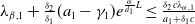


Proof. It follows from the comparison principle that
 \begin{equation*}0\lt u^{*}(t,x)\leq \frac {a_{1}-\gamma _{1}}{\delta _{1}}\,\,\textrm {for}\,(t,x)\in (0,T]\times [0,L).\end{equation*}
For
 $x\in [0,L]$
, let
$x\in [0,L]$
, let
 \begin{align*} \begin{aligned} m_{1}(t,x) &=\left \{ \begin{array}{l@{\hspace*{71.3pt}}l} a_{2}-\gamma _{2}-\delta _{2}c,&t\in (0,\overline {T}],\\ a_{2}-\gamma _{2},&t\in (\overline {T},T], \end{array} \right .\\ m(t,x) &=\left \{ \begin{array}{l@{\hspace*{22pt}}l} a_{2}-\gamma _{2}-\delta _{2}\left (e^{\frac {\alpha }{d_{1}}x}u^{*}+c\right )\!,&t\in (0,\overline {T}],\\[4pt] a_{2}-\gamma _{2}-\delta _{2}e^{\frac {\alpha }{d_{1}}x}u^{*},&t\in (\overline {T},T], \end{array} \right .\\ m_{2}(t,x) &=\left \{ \begin{array}{l@{\quad}l} a_{2}-\gamma _{2}-\delta _{2}\left (e^{\frac {\alpha }{d_{1}}L}\frac {a_{1}-\gamma _{1}}{\delta _{1}}+c\right )\!,&t\in (0,\overline {T}],\\[5pt] a_{2}-\gamma _{2}-\delta _{2}e^{\frac {\alpha }{d_{1}}L}\frac {a_{1}-\gamma _{1}}{\delta _{1}},&t\in (\overline {T},T]. \end{array} \right . \end{aligned} \end{align*}
Replace the linear part of (3.1) with
 $m_{1}v$
,
$m_{1}v$
,
 $mv$
and
$mv$
and
 $m_{2}v$
in each period and denote their corresponding principal eigenvalues as
$m_{2}v$
in each period and denote their corresponding principal eigenvalues as
 $\underline {\tau }_{1}$
,
$\underline {\tau }_{1}$
,
 $\tau _{1}$
and
$\tau _{1}$
and
 $\overline {\tau }_{1}$
, respectively. Since
$\overline {\tau }_{1}$
, respectively. Since
 $m_{1}\gt m\geq m_{2}$
in
$m_{1}\gt m\geq m_{2}$
in
 $(t,x)\in (0,T]\times [0,L]$
, by Lemma 2.15 in [Reference Cantrell and Cosner5], it follows that
$(t,x)\in (0,T]\times [0,L]$
, by Lemma 2.15 in [Reference Cantrell and Cosner5], it follows that
 $\underline {\tau }_{1}\lt \tau _{1}\leq \overline {\tau }_{1}$
, where
$\underline {\tau }_{1}\lt \tau _{1}\leq \overline {\tau }_{1}$
, where
 $\tau _{1}$
is the principal eigenvalue of (3.2). Also, it is found that
$\tau _{1}$
is the principal eigenvalue of (3.2). Also, it is found that
 $\underline {\tau }_{1}=\eta _{1}=\lambda _{\beta ,1}+\frac {\delta _{2}c\overline {T}}{T}$
, and so by
$\underline {\tau }_{1}=\eta _{1}=\lambda _{\beta ,1}+\frac {\delta _{2}c\overline {T}}{T}$
, and so by
 $(ii)$
in Lemma 2.2 and the existence requirement for
$(ii)$
in Lemma 2.2 and the existence requirement for
 $(u^{*}(t,x),0)$
, we have
$(u^{*}(t,x),0)$
, we have
 $\tau _{1}\gt \underline {\tau }_{1}\geq 0$
if
$\tau _{1}\gt \underline {\tau }_{1}\geq 0$
if
 $c\gt \hat {c}$
and
$c\gt \hat {c}$
and
 $T^{*}\lt T\leq T^{**}$
.
$T^{*}\lt T\leq T^{**}$
.
On the other hand, a similar calculation to that in the proof of Lemma 2.1 yields
 $\overline {\tau }_{1}=\lambda _{\beta ,1}+\delta _{2}e^{\frac {\alpha }{d_{1}}L}\frac {a_{1}-\gamma _{1}}{\delta _{1}} +\frac {\delta _{2}c\overline {T}}{T}$
, which is strictly decreasing with respect to
$\overline {\tau }_{1}=\lambda _{\beta ,1}+\delta _{2}e^{\frac {\alpha }{d_{1}}L}\frac {a_{1}-\gamma _{1}}{\delta _{1}} +\frac {\delta _{2}c\overline {T}}{T}$
, which is strictly decreasing with respect to
 $T$
. For case
$T$
. For case
 $\mathrm{(i)}$
, it follows from
$\mathrm{(i)}$
, it follows from
 $\lambda _{\beta ,1}+\frac {\delta _{2}}{\delta _{1}}(a_{1}-\gamma _{1})e^{\frac {\alpha }{d_{1}}L}\leq \frac {\delta _{2}c\lambda _{\alpha ,1}}{a_{1}+\delta _{1}c}$
that
$\lambda _{\beta ,1}+\frac {\delta _{2}}{\delta _{1}}(a_{1}-\gamma _{1})e^{\frac {\alpha }{d_{1}}L}\leq \frac {\delta _{2}c\lambda _{\alpha ,1}}{a_{1}+\delta _{1}c}$
that
 $\overline {\tau }_{1}\rightarrow \lambda _{\beta ,1}+\frac {\delta _{2}}{\delta _{1}}(a_{1}-\gamma _{1}) e^{\frac {\alpha }{d_{1}}L}-\frac {\delta _{2}c\lambda _{\alpha ,1}}{a_{1}+\delta _{1}c}\leq 0$
as
$\overline {\tau }_{1}\rightarrow \lambda _{\beta ,1}+\frac {\delta _{2}}{\delta _{1}}(a_{1}-\gamma _{1}) e^{\frac {\alpha }{d_{1}}L}-\frac {\delta _{2}c\lambda _{\alpha ,1}}{a_{1}+\delta _{1}c}\leq 0$
as
 $T\rightarrow {T^{*}}^{+}$
. While
$T\rightarrow {T^{*}}^{+}$
. While
 $\overline {\tau }_{1}\rightarrow \lambda _{\beta ,1}+\frac {\delta _{2}}{\delta _{1}}(a_{1}-\gamma _{1})e^{\frac {\alpha }{d_{1}}L}\lt 0$
as
$\overline {\tau }_{1}\rightarrow \lambda _{\beta ,1}+\frac {\delta _{2}}{\delta _{1}}(a_{1}-\gamma _{1})e^{\frac {\alpha }{d_{1}}L}\lt 0$
as
 $T\rightarrow +\infty$
. Therefore, if
$T\rightarrow +\infty$
. Therefore, if
 $T\gt T^{*}$
, we have
$T\gt T^{*}$
, we have
 $\tau _{1}\leq \overline {\tau }_{1}\lt 0$
. For case
$\tau _{1}\leq \overline {\tau }_{1}\lt 0$
. For case
 $\mathrm{(ii)}$
,
$\mathrm{(ii)}$
,
 $\lambda _{\beta ,1}+\frac {\delta _{2}}{\delta _{1}}(a_{1}-\gamma _{1})e^{\frac {\alpha }{d_{1}}L}\lt 0$
implies that
$\lambda _{\beta ,1}+\frac {\delta _{2}}{\delta _{1}}(a_{1}-\gamma _{1})e^{\frac {\alpha }{d_{1}}L}\lt 0$
implies that
 $\overline {\tau }_{1}\rightarrow \lambda _{\beta ,1}+\frac {\delta _{2}}{\delta _{1}}(a_{1}-\gamma _{1})e^{\frac {\alpha }{d_{1}}L}\lt 0$
as
$\overline {\tau }_{1}\rightarrow \lambda _{\beta ,1}+\frac {\delta _{2}}{\delta _{1}}(a_{1}-\gamma _{1})e^{\frac {\alpha }{d_{1}}L}\lt 0$
as
 $T\rightarrow +\infty$
. While
$T\rightarrow +\infty$
. While
 $\overline {\tau }_{1}\rightarrow \frac {\delta _{2}}{\delta _{1}}(a_{1}-\gamma _{1})e^{\frac {\alpha }{d_{1}}L} \gt 0$
as
$\overline {\tau }_{1}\rightarrow \frac {\delta _{2}}{\delta _{1}}(a_{1}-\gamma _{1})e^{\frac {\alpha }{d_{1}}L} \gt 0$
as
 $T\rightarrow {T^{**}}^{+}$
. Hence, there exists a unique
$T\rightarrow {T^{**}}^{+}$
. Hence, there exists a unique
 $\widehat {T}^{*}\,:\!=\,-\frac {\delta _{2}c\overline {T}}{\lambda _{\beta ,1}+\frac {\delta _{2}}{\delta _{1}}(a_{1} -\gamma _{1})e^{\frac {\alpha }{d_{1}}L}}\gt T^{**}\gt 0$
such that if
$\widehat {T}^{*}\,:\!=\,-\frac {\delta _{2}c\overline {T}}{\lambda _{\beta ,1}+\frac {\delta _{2}}{\delta _{1}}(a_{1} -\gamma _{1})e^{\frac {\alpha }{d_{1}}L}}\gt T^{**}\gt 0$
such that if
 $T=\widehat {T}^{*}$
, we have
$T=\widehat {T}^{*}$
, we have
 $\overline {\tau }_{1}=0$
. Notice that
$\overline {\tau }_{1}=0$
. Notice that
 $T\gt T^{*}$
is required to make
$T\gt T^{*}$
is required to make
 $(u^{*}(t,x),0)$
exist. Therefore, if
$(u^{*}(t,x),0)$
exist. Therefore, if
 $T\gt \max \{T^{*},\widehat {T}^{*}\}$
, then
$T\gt \max \{T^{*},\widehat {T}^{*}\}$
, then
 $\tau _{1}\leq \overline {\tau }_{1}\lt 0$
. We complete the proof.
$\tau _{1}\leq \overline {\tau }_{1}\lt 0$
. We complete the proof.
Lemma 3.2.
If
 $\frac {a_{1}}{\delta _{1}}\leq -\frac {\lambda _{\beta ,1}}{\delta _{2}}$
,
$\frac {a_{1}}{\delta _{1}}\leq -\frac {\lambda _{\beta ,1}}{\delta _{2}}$
,
 $c\in [\frac {a_{1}}{\delta _{1}},-\frac {\lambda _{\beta ,1}}{\delta _{2}}]$
and
$c\in [\frac {a_{1}}{\delta _{1}},-\frac {\lambda _{\beta ,1}}{\delta _{2}}]$
and
 $T\leq T^{*}$
, or if
$T\leq T^{*}$
, or if
 $T^{**}\lt T^{*}$
,
$T^{**}\lt T^{*}$
,
 $T^{**}\lt T\leq T^{*}$
and
$T^{**}\lt T\leq T^{*}$
and
 $c\gt \hat {c}$
, then
$c\gt \hat {c}$
, then
 $\sigma _{1}\gt 0$
. Assume that
$\sigma _{1}\gt 0$
. Assume that
 $\lambda _{\alpha ,1}+\frac {\xi _{1}}{\xi _{2}}(a_{2}-\gamma _{2})e^{\frac {\beta }{d_{2}}L}\lt 0$
and
$\lambda _{\alpha ,1}+\frac {\xi _{1}}{\xi _{2}}(a_{2}-\gamma _{2})e^{\frac {\beta }{d_{2}}L}\lt 0$
and
 \begin{equation*}\widehat {T}^{**}\,:\!=\,-\frac {(a_{1}+\delta _{1}c)\overline {T}}{\lambda _{\alpha ,1}+\frac {\xi _{1}}{\xi _{2}} (a_{2}-\gamma _{2})e^{\frac {\beta }{d_{2}}L}}\gt T^{*}\gt 0.\end{equation*}
Then,
 $\sigma _{1}\lt 0$
if one of the following conditions is satisfied:
$\sigma _{1}\lt 0$
if one of the following conditions is satisfied:
-
(i)
$\frac {a_{1}}{\delta _{1}}\leq -\frac {\lambda _{\beta ,1}}{\delta _{2}}$
,
$c\in [\frac {a_{1}}{\delta _{1}},-\frac {\lambda _{\beta ,1}}{\delta _{2}}]$
and
$T\gt \widehat {T}^{**}$
; -
(ii)
$c\gt \hat {c}$
and
$T\gt \max \{T^{**},\widehat {T}^{**}\}$
.


Proof. By the comparison principle, one have
 \begin{equation*}0\lt v^{*}(t,x)\leq \frac {a_{2}-\gamma _{2}}{\xi _{2}}\,\,\textrm {for}\,(t,x)\in (0,T]\times [0,L).\end{equation*}
Similarly to the proof of Lemma 3.1, we can easily obtain
 $\underline {\sigma }_{1}\lt \sigma _{1}\leq \overline {\sigma }_{1}$
by deflation, where
$\underline {\sigma }_{1}\lt \sigma _{1}\leq \overline {\sigma }_{1}$
by deflation, where
 $\sigma _{1}$
is the principal eigenvalue of (3.4) and
$\sigma _{1}$
is the principal eigenvalue of (3.4) and
 $\underline {\sigma }_{1}=\mu _{1}=\lambda _{\alpha ,1}+\frac {(a_{1}+\delta _{1}c)\overline {T}}{T}$
. Thus, by Lemma 2.1, Theorem 2.1, and the existence requirement for
$\underline {\sigma }_{1}=\mu _{1}=\lambda _{\alpha ,1}+\frac {(a_{1}+\delta _{1}c)\overline {T}}{T}$
. Thus, by Lemma 2.1, Theorem 2.1, and the existence requirement for
 $(0,u^{*}(t,x))$
, it follows that if
$(0,u^{*}(t,x))$
, it follows that if
 $c\in [\frac {a_{1}}{\delta _{1}},-\frac {\lambda _{\beta ,1}}{\delta _{2}}]$
and
$c\in [\frac {a_{1}}{\delta _{1}},-\frac {\lambda _{\beta ,1}}{\delta _{2}}]$
and
 $T\leq T^{*}$
, or
$T\leq T^{*}$
, or
 $c\gt \hat {c}$
and
$c\gt \hat {c}$
and
 $T^{**}\lt T\leq T^{*}$
, then
$T^{**}\lt T\leq T^{*}$
, then
 $\sigma _{1}\gt \underline {\sigma }_{1}\geq 0$
. Moreover,
$\sigma _{1}\gt \underline {\sigma }_{1}\geq 0$
. Moreover,
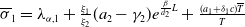 $\overline {\sigma }_{1}=\lambda _{\alpha ,1}+\frac {\xi _{1}}{\xi _{2}}(a_{2}-\gamma _{2})e^{\frac {\beta }{d_{2}}L}+\frac {(a_{1}+\delta _{1}c)\overline {T}}{T}$
, which is strictly decreasing with respect to
$\overline {\sigma }_{1}=\lambda _{\alpha ,1}+\frac {\xi _{1}}{\xi _{2}}(a_{2}-\gamma _{2})e^{\frac {\beta }{d_{2}}L}+\frac {(a_{1}+\delta _{1}c)\overline {T}}{T}$
, which is strictly decreasing with respect to
 $T$
. Since
$T$
. Since
 $\lambda _{\alpha ,1}+\frac {\xi _{1}}{\xi _{2}}(a_{2}-\gamma _{2})e^{\frac {\beta }{d_{2}}L}\lt 0$
, we have
$\lambda _{\alpha ,1}+\frac {\xi _{1}}{\xi _{2}}(a_{2}-\gamma _{2})e^{\frac {\beta }{d_{2}}L}\lt 0$
, we have
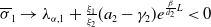 $\overline {\sigma }_{1}\rightarrow \lambda _{\alpha ,1}+\frac {\xi _{1}}{\xi _{2}}(a_{2}-\gamma _{2})e^{\frac {\beta }{d_{2}}L}\lt 0$
as
$\overline {\sigma }_{1}\rightarrow \lambda _{\alpha ,1}+\frac {\xi _{1}}{\xi _{2}}(a_{2}-\gamma _{2})e^{\frac {\beta }{d_{2}}L}\lt 0$
as
 $T\rightarrow +\infty$
. Moreover,
$T\rightarrow +\infty$
. Moreover,
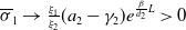 $\overline {\sigma }_{1}\rightarrow \frac {\xi _{1}}{\xi _{2}}(a_{2}-\gamma _{2})e^{\frac {\beta }{d_{2}}L}\gt 0$
as
$\overline {\sigma }_{1}\rightarrow \frac {\xi _{1}}{\xi _{2}}(a_{2}-\gamma _{2})e^{\frac {\beta }{d_{2}}L}\gt 0$
as
 $T\rightarrow {T^{*}}^{+}$
. Hence, there exists a unique
$T\rightarrow {T^{*}}^{+}$
. Hence, there exists a unique
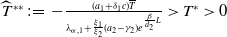 $\widehat {T}^{**}\,:\!=\,-\frac {(a_{1}+\delta _{1}c)\overline {T}}{\lambda _{\alpha ,1}+\frac {\xi _{1}}{\xi _{2}} (a_{2}-\gamma _{2})e^{\frac {\beta }{d_{2}}L}}\gt T^{*}\gt 0$
such that if
$\widehat {T}^{**}\,:\!=\,-\frac {(a_{1}+\delta _{1}c)\overline {T}}{\lambda _{\alpha ,1}+\frac {\xi _{1}}{\xi _{2}} (a_{2}-\gamma _{2})e^{\frac {\beta }{d_{2}}L}}\gt T^{*}\gt 0$
such that if
 $T=\widehat {T}^{**}$
, we have
$T=\widehat {T}^{**}$
, we have
 $\overline {\sigma }_{1}=0$
. Therefore, we can similarly obtain the conclusion. This completes the proof.
$\overline {\sigma }_{1}=0$
. Therefore, we can similarly obtain the conclusion. This completes the proof.
Now, we employ the parameters
 $c$
and
$c$
and
 $T$
to give the dynamical behaviour of system (1.4) under specific conditions.
$T$
to give the dynamical behaviour of system (1.4) under specific conditions.
Theorem 3.2. For time-switching system (1.4), the following statements hold:
-
(i) If
$c\gt \hat {c}$
and
$T\leq \min \{T^{*},T^{**}\}$
, then
$(0,0)$
is globally asymptotically stable.
-
(ii) If
$T^{*}\lt T^{**}$
,
$T\in (T^{*},T^{**}]$
and
$c\gt \hat {c}$
, then
$(u^{*}(t,x),0)$
is globally asymptotically stable.
-
(iii) If
$T^{**}\lt T^{*}$
,
$T\in (T^{**},T^{*}]$
and
$c\gt \hat {c}$
, or if
$\frac {a_{1}}{\delta _{1}}\leq -\frac {\lambda _{\beta ,1}}{\delta _{2}}$
,
$c\in [\frac {a_{1}}{\delta _{1}},-\frac {\lambda _{\beta ,1}}{\delta _{2}}]$
and
$T\leq T^{*}$
, then
$(0,v^{*}(t,x))$
is globally asymptotically stable.


Proof. The case
 $\mathrm{(i)}$
is clear by Theorems 2.1 and 2.2, and otherwise,
$\mathrm{(i)}$
is clear by Theorems 2.1 and 2.2, and otherwise,
 $(0,0)$
is unstable.
$(0,0)$
is unstable.
For
 $\mathrm{(ii)}$
, it follows from Theorem 3.1 and Lemma 3.1 that
$\mathrm{(ii)}$
, it follows from Theorem 3.1 and Lemma 3.1 that
 $(u^{*}(t,x),0)$
is locally asymptotically stable. Moreover, system (1.4) only has
$(u^{*}(t,x),0)$
is locally asymptotically stable. Moreover, system (1.4) only has
 $(0,0)$
and
$(0,0)$
and
 $(u^{*}(t,x),0)$
, where
$(u^{*}(t,x),0)$
, where
 $(0,0)$
is unstable. By Theorem in [Reference Zhao34], every solution will asymptotically converge to the semi-trivial periodic solution
$(0,0)$
is unstable. By Theorem in [Reference Zhao34], every solution will asymptotically converge to the semi-trivial periodic solution
 $(u^{*}(t,x),0)$
, which implies that
$(u^{*}(t,x),0)$
, which implies that
 $(u^{*}(t,x),0)$
is globally attractive. Therefore,
$(u^{*}(t,x),0)$
is globally attractive. Therefore,
 $(u^{*}(t,x),0)$
is globally asymptotically stable. The discussion for case
$(u^{*}(t,x),0)$
is globally asymptotically stable. The discussion for case
 $\mathrm{(iii)}$
is similar to Theorem 3.1, Lemma 3.2 and some global attractivity statements.
$\mathrm{(iii)}$
is similar to Theorem 3.1, Lemma 3.2 and some global attractivity statements.
Theorem 3.3.
The time-switching system (1.4) possesses at least one coexisting
 $T$
-periodic solution, and both semi-trivial
$T$
-periodic solution, and both semi-trivial
 $T$
-periodic solutions
$T$
-periodic solutions
 $(u^{*}(t,x),0)$
and
$(u^{*}(t,x),0)$
and
 $(0,v^{*}(t,x))$
are unstable when either of the following holds:
$(0,v^{*}(t,x))$
are unstable when either of the following holds:
-
(i)
$\frac {a_{1}}{\delta _{1}}\leq -\frac {\lambda _{\beta ,1}}{\delta _{2}}$
with
$c\in \left [\frac {a_{1}}{\delta _{1}},-\frac {\lambda _{\beta ,1}}{\delta _{2}}\right ]$
and
$T\gt \widehat {T}^{**}$
subject to:
\begin{equation*} \lambda _{\beta ,1}+\frac {\delta _{2}}{\delta _{1}}(a_{1}-\gamma _{1})e^{\frac {\alpha }{d_{1}}L}\leq \frac {\delta _{2}c\lambda _{\alpha ,1}}{a_{1}+\delta _{1}c}, \quad \lambda _{\alpha ,1}+\frac {\xi _{1}}{\xi _{2}}(a_{2}-\gamma _{2})e^{\frac {\beta }{d_{2}}L}\lt 0; \end{equation*}
-
(ii)
$c\gt \hat {c}$
with
$T\gt \max \{\widehat {T}^{*},\widehat {T}^{**}\}$
subject to:
\begin{equation*} \lambda _{\beta ,1}+\frac {\delta _{2}}{\delta _{1}}(a_{1}-\gamma _{1})e^{\frac {\alpha }{d_{1}}L}\lt 0, \quad \lambda _{\alpha ,1}+\frac {\xi _{1}}{\xi _{2}}(a_{2}-\gamma _{2})e^{\frac {\beta }{d_{2}}L}\lt 0. \end{equation*}


Proof. This conclusion can be obtained directly from
 $\mathrm{(iii)}$
in Theorem 3.1, Lemmas 3.1 and 3.2, so we omit the details.
$\mathrm{(iii)}$
in Theorem 3.1, Lemmas 3.1 and 3.2, so we omit the details.
Remark 3.2. In the biological sense, the global asymptotic stability of
 $(0,0)$
implies that both Aedes mosquitoes are finally eliminated. According to the conditions of
$(0,0)$
implies that both Aedes mosquitoes are finally eliminated. According to the conditions of
 $\mathrm{(i)}$
in Theorem 3.2, taking
$\mathrm{(i)}$
in Theorem 3.2, taking
 $c=\hat {c}$
and
$c=\hat {c}$
and
 $T=\widehat {T}\,:\!=\,\min \{T^{*},T^{**}\}$
, namely the minimal release amount and the maximal release period that can eliminate the mosquitoes, which is the most economical control strategy of mosquitoes. In addition, if
$T=\widehat {T}\,:\!=\,\min \{T^{*},T^{**}\}$
, namely the minimal release amount and the maximal release period that can eliminate the mosquitoes, which is the most economical control strategy of mosquitoes. In addition, if
 $T^{*}\lt T^{**}$
, then
$T^{*}\lt T^{**}$
, then
 $\textit {Ae. albopictus}$
population
$\textit {Ae. albopictus}$
population
 $u$
is said to be more competitive than
$u$
is said to be more competitive than
 $\textit {Ae. aegypti}$
population
$\textit {Ae. aegypti}$
population
 $v$
. With a compromised release frequency, as
$v$
. With a compromised release frequency, as
 $T\in (T^{*},T^{**}]$
in
$T\in (T^{*},T^{**}]$
in
 $\mathrm{(ii)}$
of Theorem 3.2 and sufficient release, namely
$\mathrm{(ii)}$
of Theorem 3.2 and sufficient release, namely
 $c\gt \hat {c}$
, then
$c\gt \hat {c}$
, then
 $(u^{*}(t,x),0)$
is globally asymptotically stable, that is, only
$(u^{*}(t,x),0)$
is globally asymptotically stable, that is, only
 $v$
is eliminated. And vice versa. Further, if the strength of the suppression is weak, such as the release frequency is so low that
$v$
is eliminated. And vice versa. Further, if the strength of the suppression is weak, such as the release frequency is so low that
 $T\gt \widehat {T}^{**}$
or
$T\gt \widehat {T}^{**}$
or
 $T\gt \max \{\widehat {T}^{*},\widehat {T}^{**}\}$
, the existence of a coexisting periodic solution in Theorem 3.3 indicates that both mosquitoes persist.
$T\gt \max \{\widehat {T}^{*},\widehat {T}^{**}\}$
, the existence of a coexisting periodic solution in Theorem 3.3 indicates that both mosquitoes persist.
The conditions in Theorem 3.3, such as
 $\lambda _{\beta ,1}+\frac {\delta _{2}}{\delta _{1}}(a_{1}-\gamma _{1})e^{\frac {\alpha }{d_{1}}L}\leq \frac {\delta _{2}c\lambda _{\alpha ,1}}{a_{1}+\delta _{1}c}$
and
$\lambda _{\beta ,1}+\frac {\delta _{2}}{\delta _{1}}(a_{1}-\gamma _{1})e^{\frac {\alpha }{d_{1}}L}\leq \frac {\delta _{2}c\lambda _{\alpha ,1}}{a_{1}+\delta _{1}c}$
and
 $\lambda _{\alpha ,1}+\frac {\xi _{1}}{\xi _{2}}(a_{2}-\gamma _{2})e^{\frac {\beta }{d_{2}}L}\lt 0$
, can be reached as long as
$\lambda _{\alpha ,1}+\frac {\xi _{1}}{\xi _{2}}(a_{2}-\gamma _{2})e^{\frac {\beta }{d_{2}}L}\lt 0$
, can be reached as long as
 $\delta _{2}$
and
$\delta _{2}$
and
 $\xi _{1}$
are sufficiently small, which is the weak competition case. The strong competition condition is absent because the signs of the principal eigenvalues
$\xi _{1}$
are sufficiently small, which is the weak competition case. The strong competition condition is absent because the signs of the principal eigenvalues
 $\tau _{1}$
and
$\tau _{1}$
and
 $\sigma _{1}$
are discussed utilising the deflation and comparison methods.
$\sigma _{1}$
are discussed utilising the deflation and comparison methods.
4. Numerical simulations
In this section, we give some numerical examples to confirm the results in Theorems 3.2 and 3.3. Fix
 $d_{1}=0.15,\,d_{2}=0.1,\alpha =\beta =b=0,\,L=2\pi ,\,\overline {T}=3,\,\gamma _{1}=0.2,\,\gamma _{2}=0.3,\,\xi _{1}=\xi _{2}=0.2$
.
$d_{1}=0.15,\,d_{2}=0.1,\alpha =\beta =b=0,\,L=2\pi ,\,\overline {T}=3,\,\gamma _{1}=0.2,\,\gamma _{2}=0.3,\,\xi _{1}=\xi _{2}=0.2$
.
Example 4.1. Let
 \begin{equation*}a_{1}=8,\,a_{2}=3,\,\delta _1=0.3,\,\delta _2=0.3,\,c=28.\end{equation*}
Then, a calculation gives
 $c\gt \hat {c}\approx 26.667$
and
$c\gt \hat {c}\approx 26.667$
and
 $T^{*}\approx 6.308\lt T^{**}\approx 9.333$
. If we choose
$T^{*}\approx 6.308\lt T^{**}\approx 9.333$
. If we choose
 $T=5$
, then
$T=5$
, then
 $\mathrm{(i)}$
in Theorem
3.2
is satisfied, and
$\mathrm{(i)}$
in Theorem
3.2
is satisfied, and
 $(0,0)$
is globally asymptotically stable, as shown in the upper two pictures in Figure
1
. While if
$(0,0)$
is globally asymptotically stable, as shown in the upper two pictures in Figure
1
. While if
 $T=9$
, then we have
$T=9$
, then we have
 $T\in (T^{*},T^{**}]$
, as shown in the lower two pictures in Figure
1
,
$T\in (T^{*},T^{**}]$
, as shown in the lower two pictures in Figure
1
,
 $u$
converges to a positive periodic solution and
$u$
converges to a positive periodic solution and
 $v$
converges to 0, which is consistent with
$v$
converges to 0, which is consistent with
 $\mathrm{(ii)}$
in Theorem
3.2
. The initial value in Figure
1
is chosen as
$\mathrm{(ii)}$
in Theorem
3.2
. The initial value in Figure
1
is chosen as
 $(u_{0},v_{0})=(2,2)$
for
$(u_{0},v_{0})=(2,2)$
for
 $x\in [0,L]$
.
$x\in [0,L]$
.
For visualisation and higher persuasion, we give the profiles intercepted at the position
 $x=0$
for different initial values. Specifically, taking
$x=0$
for different initial values. Specifically, taking
 $T=5$
in Figure
2
and
$T=5$
in Figure
2
and
 $T=9$
in Figure
3
, respectively, we simulate the cases with the three initial values
$T=9$
in Figure
3
, respectively, we simulate the cases with the three initial values
 $(u_{0},v_{0})=(1,3)$
(red line),
$(u_{0},v_{0})=(1,3)$
(red line),
 $(u_{0},v_{0})=(2,2)$
(blue line) and
$(u_{0},v_{0})=(2,2)$
(blue line) and
 $(u_{0},v_{0})=(3,1)$
(black line) for
$(u_{0},v_{0})=(3,1)$
(black line) for
 $x\in [0,L]$
. It is found that they all satisfy the conclusion of Theorem
3.2
.
$x\in [0,L]$
. It is found that they all satisfy the conclusion of Theorem
3.2
.
The evolutions of
 $u$
and
$u$
and
 $v$
, where
$v$
, where
 $T=5$
in the upper two pictures and
$T=5$
in the upper two pictures and
 $T=9$
in the lower two. The initial value is
$T=9$
in the lower two. The initial value is
 $(u_{0},v_{0})=(2,2)$
for
$(u_{0},v_{0})=(2,2)$
for
 $x\in [0,L]$
. See Example 4.1 for the values of the other parameters.
$x\in [0,L]$
. See Example 4.1 for the values of the other parameters.

The evolutions of the profiles of
 $u$
and
$u$
and
 $v$
, intercepted at
$v$
, intercepted at
 $x=0$
. Here,
$x=0$
. Here,
 $T=5$
, and the initial values
$T=5$
, and the initial values
 $(u_{0},v_{0})=(1,3)$
(red line),
$(u_{0},v_{0})=(1,3)$
(red line),
 $(u_{0},v_{0})=(2,2)$
(blue line) and
$(u_{0},v_{0})=(2,2)$
(blue line) and
 $(u_{0},v_{0})=(3,1)$
(black line) for
$(u_{0},v_{0})=(3,1)$
(black line) for
 $x\in [0,L]$
. See Example 4.1 for the values of the other parameters.
$x\in [0,L]$
. See Example 4.1 for the values of the other parameters.

The evolutions of the profiles of
 $u$
and
$u$
and
 $v$
, intercepted at
$v$
, intercepted at
 $x=0$
. Here,
$x=0$
. Here,
 $T=9$
, and the initial values
$T=9$
, and the initial values
 $(u_{0},v_{0})=(1,3)$
(red line),
$(u_{0},v_{0})=(1,3)$
(red line),
 $(u_{0},v_{0})=(2,2)$
(blue line) and
$(u_{0},v_{0})=(2,2)$
(blue line) and
 $(u_{0},v_{0})=(3,1)$
(black line) for
$(u_{0},v_{0})=(3,1)$
(black line) for
 $x\in [0,L]$
. See Example 4.1 for the values of the other parameters.
$x\in [0,L]$
. See Example 4.1 for the values of the other parameters.

Example 4.2. Let
 \begin{equation*}a_{1}=8,\,a_{2}=5,\,\delta _1=0.35,\,\delta _2=0.25,\,c=28.\end{equation*}
Then, we have
 $c\gt \hat {c}\approx 22.857$
and
$c\gt \hat {c}\approx 22.857$
and
 $T^{**}\approx 4.468\lt T^{*}\approx 6.846$
. If
$T^{**}\approx 4.468\lt T^{*}\approx 6.846$
. If
 $T=4$
, then
$T=4$
, then
 $T\lt \min \{T^{*},T^{**}\}$
, and
$T\lt \min \{T^{*},T^{**}\}$
, and
 $(0,0)$
is globally asymptotically stable according to
$(0,0)$
is globally asymptotically stable according to
 $\mathrm{(i)}$
in Theorem
3.2
. As shown in Figure
4
, both
$\mathrm{(i)}$
in Theorem
3.2
. As shown in Figure
4
, both
 $u$
and
$u$
and
 $v$
asymptotically converge to 0 for various initial values
$v$
asymptotically converge to 0 for various initial values
 $(u_{0},v_{0})=(0.1,0.3)$
(red line),
$(u_{0},v_{0})=(0.1,0.3)$
(red line),
 $(u_{0},v_{0})=(0.2,0.2)$
(blue line) and
$(u_{0},v_{0})=(0.2,0.2)$
(blue line) and
 $(u_{0},v_{0})=(0.3,0.1)$
(black line) for
$(u_{0},v_{0})=(0.3,0.1)$
(black line) for
 $x\in [0,L]$
. If
$x\in [0,L]$
. If
 $T=6$
, then
$T=6$
, then
 $T\in (T^{**},T^{*}]$
, which satisfies the former condition of
$T\in (T^{**},T^{*}]$
, which satisfies the former condition of
 $\mathrm{(iii)}$
in Theorem
3.2
, and Figure
5
shows that
$\mathrm{(iii)}$
in Theorem
3.2
, and Figure
5
shows that
 $u$
will tend to 0, while
$u$
will tend to 0, while
 $v$
gradually tends to a positive periodic solution under the same initial values, which is in line with the conclusion.
$v$
gradually tends to a positive periodic solution under the same initial values, which is in line with the conclusion.
The evolutions of the profiles of
 $u$
and
$u$
and
 $v$
, intercepted at
$v$
, intercepted at
 $x=0$
. Here,
$x=0$
. Here,
 $T=4$
, and the initial values
$T=4$
, and the initial values
 $(u_{0},v_{0})=(0.1,0.3)$
(red line),
$(u_{0},v_{0})=(0.1,0.3)$
(red line),
 $(u_{0},v_{0})=(0.2,0.2)$
(blue line) and
$(u_{0},v_{0})=(0.2,0.2)$
(blue line) and
 $(u_{0},v_{0})=(0.3,0.1)$
(black line) for
$(u_{0},v_{0})=(0.3,0.1)$
(black line) for
 $x\in [0,L]$
. See Example 4.2 for the values of the other parameters.
$x\in [0,L]$
. See Example 4.2 for the values of the other parameters.


Example 4.3. Let
 \begin{equation*}a_{1}=8,\,a_{2}=6,\,\delta _1=0.3.\end{equation*}
If we further take
 $\delta _{2}=0.2$
and
$\delta _{2}=0.2$
and
 $c=28$
, then
$c=28$
, then
 $\frac {a_{1}}{\delta _{1}}\approx 26.667\lt c\lt -\frac {\lambda _{\beta ,1}}{\delta _{2}}=28.5$
and
$\frac {a_{1}}{\delta _{1}}\approx 26.667\lt c\lt -\frac {\lambda _{\beta ,1}}{\delta _{2}}=28.5$
and
 $T^{*}\approx 6.308$
. So, if we take
$T^{*}\approx 6.308$
. So, if we take
 $T=6$
, the latter condition of
$T=6$
, the latter condition of
 $\mathrm{(iii)}$
in Theorem
3.2
is satisfied, as shown in Figure
6
with initial values
$\mathrm{(iii)}$
in Theorem
3.2
is satisfied, as shown in Figure
6
with initial values
 $(u_{0},v_{0})=(1,3)$
(red line),
$(u_{0},v_{0})=(1,3)$
(red line),
 $(u_{0},v_{0})=(2,2)$
(blue line) and
$(u_{0},v_{0})=(2,2)$
(blue line) and
 $(u_{0},v_{0})=(3,1)$
(black line) for
$(u_{0},v_{0})=(3,1)$
(black line) for
 $x\in [0,L]$
,
$x\in [0,L]$
,
 $u$
will tend to 0, while
$u$
will tend to 0, while
 $v$
tends to a positive periodic solution, consistent with the conclusion.
$v$
tends to a positive periodic solution, consistent with the conclusion.
To simulate the two conclusions of Theorem
3.3
, take
 $\delta _{2}=0.1,c=28$
for
$\delta _{2}=0.1,c=28$
for
 $\mathrm{(i)}$
and
$\mathrm{(i)}$
and
 $\delta _{2}=0.2,c=30$
for
$\delta _{2}=0.2,c=30$
for
 $\mathrm{(ii)}$
, respectively, then it is calculated that
$\mathrm{(ii)}$
, respectively, then it is calculated that
 $\frac {a_{1}}{\delta _{1}}\approx 26.667\lt c\lt -\frac {\lambda _{\beta ,1}}{\delta _{2}}=57$
and
$\frac {a_{1}}{\delta _{1}}\approx 26.667\lt c\lt -\frac {\lambda _{\beta ,1}}{\delta _{2}}=57$
and
 $\widehat {T}^{**}\approx 23.429$
for
$\widehat {T}^{**}\approx 23.429$
for
 $\mathrm{(i)}$
and
$\mathrm{(i)}$
and
 $c\gt \hat {c}=28.5$
,
$c\gt \hat {c}=28.5$
,
 $\widehat {T}^{*}=36$
and
$\widehat {T}^{*}=36$
and
 $\widehat {T}^{**}\approx 24.286$
for
$\widehat {T}^{**}\approx 24.286$
for
 $\mathrm{(ii)}$
, respectively. In addition, it is easily found that its corresponding weak competition condition is satisfied. We simulate the evolution results for taking different suitable
$\mathrm{(ii)}$
, respectively. In addition, it is easily found that its corresponding weak competition condition is satisfied. We simulate the evolution results for taking different suitable
 $T$
values with fixed initial values. Specifically, taking
$T$
values with fixed initial values. Specifically, taking
 $T=30$
(red line),
$T=30$
(red line),
 $T=36$
(blue line) and
$T=36$
(blue line) and
 $T=42$
(black line) for
$T=42$
(black line) for
 $\mathrm{(i)}$
with
$\mathrm{(i)}$
with
 $(u_{0},v_{0})=(2,2)$
and taking
$(u_{0},v_{0})=(2,2)$
and taking
 $T=38$
(red line),
$T=38$
(red line),
 $T=44$
(blue line) and
$T=44$
(blue line) and
 $T=50$
(black line) for
$T=50$
(black line) for
 $\mathrm{(ii)}$
with
$\mathrm{(ii)}$
with
 $(u_{0},v_{0})=(4,4)$
, as shown in Figures
7
and
8
, respectively, both
$(u_{0},v_{0})=(4,4)$
, as shown in Figures
7
and
8
, respectively, both
 $u$
and
$u$
and
 $v$
converge to a positive periodic solution, which indicates that the two species coexist, conforming to the conclusion of
$v$
converge to a positive periodic solution, which indicates that the two species coexist, conforming to the conclusion of
 $\mathrm{(i)}$
and
$\mathrm{(i)}$
and
 $\mathrm{(ii)}$
, respectively, in Theorem
3.3
.
$\mathrm{(ii)}$
, respectively, in Theorem
3.3
.
The evolutions of the profiles of
 $u$
and
$u$
and
 $v$
, intercepted at
$v$
, intercepted at
 $x=0$
. Here,
$x=0$
. Here,
 $T=6$
, and the initial values
$T=6$
, and the initial values
 $(u_{0},v_{0})=(1,3)$
(red line),
$(u_{0},v_{0})=(1,3)$
(red line),
 $(u_{0},v_{0})=(2,2)$
(blue line) and
$(u_{0},v_{0})=(2,2)$
(blue line) and
 $(u_{0},v_{0})=(3,1)$
(black line) for
$(u_{0},v_{0})=(3,1)$
(black line) for
 $x\in [0,L]$
. See Example 4.3 for the values of the other parameters.
$x\in [0,L]$
. See Example 4.3 for the values of the other parameters.

The evolutions of the profiles of
 $u$
and
$u$
and
 $v$
, intercepted at
$v$
, intercepted at
 $x=0$
. Here
$x=0$
. Here
 $T=30$
(red line),
$T=30$
(red line),
 $T=36$
(blue line) and
$T=36$
(blue line) and
 $T=42$
(black line), and the initial value
$T=42$
(black line), and the initial value
 $(u_{0},v_{0})=(2,2)$
for
$(u_{0},v_{0})=(2,2)$
for
 $x\in [0,L]$
. See Example 4.3 for the values of the other parameters.
$x\in [0,L]$
. See Example 4.3 for the values of the other parameters.

The evolutions of the profiles of
 $u$
and
$u$
and
 $v$
, intercepted at
$v$
, intercepted at
 $x=0$
. Here,
$x=0$
. Here,
 $T=38$
(red line),
$T=38$
(red line),
 $T=44$
(blue line) and
$T=44$
(blue line) and
 $T=50$
(black line), and the initial value
$T=50$
(black line), and the initial value
 $(u_{0},v_{0})=(4,4)$
for
$(u_{0},v_{0})=(4,4)$
for
 $x\in [0,L]$
. See Example 4.3 for the values of the other parameters.
$x\in [0,L]$
. See Example 4.3 for the values of the other parameters.

5. Concluding remarks
In this paper, we develop and study a time-switching reaction-diffusion-advection system based on competition between
 $\textit {Ae. albopictus}$
(denoted as
$\textit {Ae. albopictus}$
(denoted as
 $u$
) and
$u$
) and
 $\textit {Ae. aegypti}$
(denoted as
$\textit {Ae. aegypti}$
(denoted as
 $v$
). Only sterile mosquitoes of
$v$
). Only sterile mosquitoes of
 $\textit {Ae. albopictus}$
-type are released to suppress field mosquitoes with the release amount, sexually lifespan and release period being
$\textit {Ae. albopictus}$
-type are released to suppress field mosquitoes with the release amount, sexually lifespan and release period being
 $c$
,
$c$
,
 $\overline {T}$
and
$\overline {T}$
and
 $T$
, respectively. We consider the case of
$T$
, respectively. We consider the case of
 $\overline {T}\lt T$
, by which time-switching occurs. The periodic dynamics of the system are discussed by the eigenvalue method and the upper and lower solution method, in terms of the two key parameters
$\overline {T}\lt T$
, by which time-switching occurs. The periodic dynamics of the system are discussed by the eigenvalue method and the upper and lower solution method, in terms of the two key parameters
 $c$
and
$c$
and
 $T$
. This answers the critical questions of how many sterile mosquitoes are released at a time and how often to release them to eliminate the wild mosquitoes. Specifically, the corresponding single switching equations for
$T$
. This answers the critical questions of how many sterile mosquitoes are released at a time and how often to release them to eliminate the wild mosquitoes. Specifically, the corresponding single switching equations for
 $u$
and
$u$
and
 $v$
are first discussed separately, giving the thresholds
$v$
are first discussed separately, giving the thresholds
 $T^*$
and
$T^*$
and
 $T^{**}$
that determine whether they are persistent or not, as well as the minimal release amount
$T^{**}$
that determine whether they are persistent or not, as well as the minimal release amount
 $\hat {c}$
that can exterminate mosquitoes. Then, we discuss the dynamics of system (1.4). By analysing the eigenvalue problems of the linearised equations of the systems at the two semi-trivial
$\hat {c}$
that can exterminate mosquitoes. Then, we discuss the dynamics of system (1.4). By analysing the eigenvalue problems of the linearised equations of the systems at the two semi-trivial
 $T$
-periodic solutions
$T$
-periodic solutions
 $(u^{*}(t,x),0)$
and
$(u^{*}(t,x),0)$
and
 $(0,v^{*}(t,x))$
, respectively, two further thresholds
$(0,v^{*}(t,x))$
, respectively, two further thresholds
 $\widehat {T}^*$
and
$\widehat {T}^*$
and
 $\widehat {T}^{**}$
are defined, which in combination with the previous conditions give the dynamics of system (1.4) (see Theorems 3.2 and 3.3). Therein, the global asymptotic stability of the trivial steady state and semi-trivial
$\widehat {T}^{**}$
are defined, which in combination with the previous conditions give the dynamics of system (1.4) (see Theorems 3.2 and 3.3). Therein, the global asymptotic stability of the trivial steady state and semi-trivial
 $T$
-periodic solutions are analysed, and the existence of a coexisting
$T$
-periodic solutions are analysed, and the existence of a coexisting
 $T$
-periodic solution of the system is obtained.
$T$
-periodic solution of the system is obtained.
In recent years, time-switching mathematical models based on the use of biotechnology to eradicate mosquitoes have emerged, but most of them focus on non-spatial models, ignoring the key spatial factors affecting mosquito propagation such as wind speed, habitat size and quality, to name a few. In fact, if the dynamics of system (1.4) are given in terms of the parameters
 $\alpha$
and
$\alpha$
and
 $\beta$
, the critical effect of wind speed on the reproduction and propagation of mosquito populations is well represented. For fixed-scale mosquito factories, the planning of production and release of sterile mosquitoes usually remains unchanged, which implies that the amount of release
$\beta$
, the critical effect of wind speed on the reproduction and propagation of mosquito populations is well represented. For fixed-scale mosquito factories, the planning of production and release of sterile mosquitoes usually remains unchanged, which implies that the amount of release
 $c$
and the release period
$c$
and the release period
 $T$
may be fixed. Thus, it is important to examine the wind speed at the release site. It follows from Proposition 2.1 in [Reference Lou and Zhou18], the principal eigenvalue
$T$
may be fixed. Thus, it is important to examine the wind speed at the release site. It follows from Proposition 2.1 in [Reference Lou and Zhou18], the principal eigenvalue
 $\lambda _{\alpha ,1}$
of (2.4) is strictly increasing with respect to
$\lambda _{\alpha ,1}$
of (2.4) is strictly increasing with respect to
 $\alpha$
and satisfies
$\alpha$
and satisfies
 $\lim _{\alpha \rightarrow 0}\lambda _{\alpha ,1}=-(a_{1}-\gamma _{1})\lt 0$
and
$\lim _{\alpha \rightarrow 0}\lambda _{\alpha ,1}=-(a_{1}-\gamma _{1})\lt 0$
and
 $\lim _{\alpha \rightarrow +\infty }\lambda _{\alpha ,1}=+\infty$
(the assumption that
$\lim _{\alpha \rightarrow +\infty }\lambda _{\alpha ,1}=+\infty$
(the assumption that
 $\lambda _{\alpha ,1}\lt 0$
is no longer needed here). Thus, for the principal eigenvalue
$\lambda _{\alpha ,1}\lt 0$
is no longer needed here). Thus, for the principal eigenvalue
 $\mu _{1}$
of (2.2), we compute as
$\mu _{1}$
of (2.2), we compute as
 \begin{equation*}\mu _{1}=\lambda _{\alpha ,1}+\frac {(a_{1}+\delta _{1}c)\overline {T}}{T}.\end{equation*}
As long as the parameters other than
 $\alpha$
are fixed and satisfy
$\alpha$
are fixed and satisfy
 $(a_{1}+\delta _{1}c)\overline {T}\lt (a_{1}-\gamma _{1})T$
, we have that
$(a_{1}+\delta _{1}c)\overline {T}\lt (a_{1}-\gamma _{1})T$
, we have that
 $\mu _{1}\rightarrow \frac {(a_{1}+\delta _{1}c)\overline {T}}{T}-(a_{1}-\gamma _{1})\lt 0$
as
$\mu _{1}\rightarrow \frac {(a_{1}+\delta _{1}c)\overline {T}}{T}-(a_{1}-\gamma _{1})\lt 0$
as
 $\alpha \rightarrow 0$
and
$\alpha \rightarrow 0$
and
 $\mu _{1}\gt 0$
as
$\mu _{1}\gt 0$
as
 $\alpha \rightarrow +\infty$
. Therefore, there exists a unique
$\alpha \rightarrow +\infty$
. Therefore, there exists a unique
 $\alpha ^{*}$
such that if
$\alpha ^{*}$
such that if
 $\alpha =\alpha ^{*}$
, we have
$\alpha =\alpha ^{*}$
, we have
 $\mu _{1}=0$
. Further, if
$\mu _{1}=0$
. Further, if
 $\alpha \gt \alpha ^{*}$
, then
$\alpha \gt \alpha ^{*}$
, then
 $\mu _{1}\gt 0$
, while if
$\mu _{1}\gt 0$
, while if
 $\alpha \lt \alpha ^{*}$
, then
$\alpha \lt \alpha ^{*}$
, then
 $\mu _{1}\lt 0$
. Similar to the analysis of Lemma 2.1 and Theorem 2.1, if
$\mu _{1}\lt 0$
. Similar to the analysis of Lemma 2.1 and Theorem 2.1, if
 $\alpha \gt \alpha ^{*}$
, in this case we call the wind speed higher, the steady state 0 of (2.1) is globally attractive, namely, the population
$\alpha \gt \alpha ^{*}$
, in this case we call the wind speed higher, the steady state 0 of (2.1) is globally attractive, namely, the population
 $u$
will eventually become extinct. Conversely, if
$u$
will eventually become extinct. Conversely, if
 $\alpha \lt \alpha ^{*}$
, then population
$\alpha \lt \alpha ^{*}$
, then population
 $u$
will persist, indicating that Ae. albopictus
$u$
will persist, indicating that Ae. albopictus
 $u$
cannot be eliminated under the current release strategy and weaker wind speed conditions. Similarly, for the Ae. aegypti population
$u$
cannot be eliminated under the current release strategy and weaker wind speed conditions. Similarly, for the Ae. aegypti population
 $v$
, a threshold
$v$
, a threshold
 $\beta ^{*}$
can be defined that, in combination with the conditions for
$\beta ^{*}$
can be defined that, in combination with the conditions for
 $\alpha ^{*}$
, gives the global dynamics of (1.4) and reveal the key factors that can eradicate mosquito populations.
$\alpha ^{*}$
, gives the global dynamics of (1.4) and reveal the key factors that can eradicate mosquito populations.
As mentioned before, Ae. albopictus and Ae. aegypti mosquitoes are the two most damaging Aedes mosquitoes and extensive competition exists between them. If the interactions between them are ignored, the model of suppression of either Aedes is not convincing, because the unsuppressed population of another Aedes may expand unchecked and continue to transmit mosquito-borne diseases. Furthermore, competing systems exhibit richer dynamical properties, and there is currently less relevant work on time period switching reaction-diffusion systems. In this paper, we present a reaction-diffusion-advection system to accurately describe the temporal and spatial evolution of mosquito populations, providing effective assistance for the development of rational mosquito control measures and bringing inspiration to the study of time-switching spatial systems.
Financial support
The research was supported partially by the National Natural Science Foundation of China [12331017, 12471458, 12171110], the Natural Sciences and Engineering Research Council of Canada [RGPIN-2019-05892, RGPIN-2024-05593] and the Basic and Applied Basic Research Foundation of Guangdong Province [2023A1515011110].
Competing interests
The authors declare none.


 Open access