





1. Introduction
The spreading of a localised bolus of chemical in a pipe or channel flow of a Newtonian fluid with constant viscosity $\mu _N$
involves the interplay of the velocity profile, with average speed
$\mu _N$
involves the interplay of the velocity profile, with average speed $\langle u\rangle$
, and the Brownian motion, or effective diffusion constant,
$\langle u\rangle$
, and the Brownian motion, or effective diffusion constant, $D_N$
, of the solute. The spreading of solute is usually dominated by the flow as the velocity varies across a channel, thus acting to increase the distance between solute near the walls, in contrast to solute near the centre of the channel. In the case of laminar flows, Taylor (Reference Taylor1953) and Aris (Reference Aris1956), following distinct approaches, described the long-time behaviour of a spreading solute in pressure-driven flow in uniform channels in terms of an effective (Taylor–Aris) axial dispersion coefficient,
$D_N$
, of the solute. The spreading of solute is usually dominated by the flow as the velocity varies across a channel, thus acting to increase the distance between solute near the walls, in contrast to solute near the centre of the channel. In the case of laminar flows, Taylor (Reference Taylor1953) and Aris (Reference Aris1956), following distinct approaches, described the long-time behaviour of a spreading solute in pressure-driven flow in uniform channels in terms of an effective (Taylor–Aris) axial dispersion coefficient, $D_{\textit {eff}}$
, that exceeds that of molecular diffusion by an amount proportional to
$D_{\textit {eff}}$
, that exceeds that of molecular diffusion by an amount proportional to $\langle u\rangle ^2 a^2/ D_N$
, where
$\langle u\rangle ^2 a^2/ D_N$
, where $a$
is the pipe radius or channel height (Taylor Reference Taylor1953; Aris Reference Aris1956). The enhanced spreading occurs because solute molecules can diffuse from fast streamlines to slow streamlines, and vice versa, with larger diffusion constants tending to make the solute distribution more uniform, thus reducing the dispersion coefficient.
$a$
is the pipe radius or channel height (Taylor Reference Taylor1953; Aris Reference Aris1956). The enhanced spreading occurs because solute molecules can diffuse from fast streamlines to slow streamlines, and vice versa, with larger diffusion constants tending to make the solute distribution more uniform, thus reducing the dispersion coefficient.
Complex, non-Newtonian fluids can have a shear-rate-dependent viscosity, which changes the velocity profile, even in simple geometries such as pressure-driven pipe or channel flow. For example, common inelastic constitutive equations relating the strain rate to the stress, such as power-law, Ellis, Carreau and Casson models, as well as viscoelastic descriptions, such as Phan-Thien–Tanner, Giesekus and a finitely extensible nonlinear elastic (FENE) model with the Peterlin approximation (FENE-P), all display a shear-rate-dependent viscosity (Bird, Armstrong & Hassager Reference Bird, Armstrong and Hassager1987). Because the velocity profile changes across the channel, a change in the dispersion coefficient is expected. We note that for the Oldroyd-B and FENE-CR models, there is no shear thinning and no change in the velocity profile from that of a Newtonian fluid for fully developed pressure-driven flow in a straight channel (see, e.g. Mahapatra et al. Reference Mahapatra, Ruangkriengsin, Stone and Boyko2025).
There are many studies in the literature, spanning at least the past six decades, that describe the flow-enhanced contribution to solute dispersion in complex fluids (Fan & Hwang Reference Fan and Hwang1965; Booras & Krantz Reference Booras and Krantz1976; Sharp Reference Sharp1993; Dash, Jayaraman & Mehta Reference Dash, Jayaraman and Mehta2000; Nagarani & Sebastian Reference Nagarani and Sebastian2013; Rana & Murthy Reference Rana and Murthy2016a
,
Reference Rana and Murthyb
; Singh & Murthy Reference Singh and Murthy2023; Teodoro, Bautista & Méndez Reference Teodoro, Bautista and Méndez2025). Nevertheless, the corresponding dispersion coefficient of a colloidal solute also depends on the background particle diffusivity, which itself should be expected to depend on the local viscosity, in which case it would also depend on the shear rate; i.e. the diffusion coefficient that forms the basis for sampling the velocity distribution changes from $D_N$
. In particular, for a constant viscosity Newtonian solvent (
$D_N$
. In particular, for a constant viscosity Newtonian solvent ( $\mu _N$
) and a solute with effective radius
$\mu _N$
) and a solute with effective radius $b$
, the Stokes–Einstein relation is
$b$
, the Stokes–Einstein relation is $D_N = k_BT/(6\pi b \mu _N)$
, where
$D_N = k_BT/(6\pi b \mu _N)$
, where $k_{B}$
is the Boltzmann constant and
$k_{B}$
is the Boltzmann constant and $T$
is the temperature. Denoting the local shear rate as
$T$
is the temperature. Denoting the local shear rate as $\dot \gamma$
, then, since we consider a shear-rate-dependent viscosity,
$\dot \gamma$
, then, since we consider a shear-rate-dependent viscosity, $\mu ({\dot \gamma } )$
, we expect for particles large compared with the typical polymer length scales (see § 2.3) the corresponding diffusion coefficient
$\mu ({\dot \gamma } )$
, we expect for particles large compared with the typical polymer length scales (see § 2.3) the corresponding diffusion coefficient $D$
to be inversely related to
$D$
to be inversely related to $\mu ({\dot \gamma } )$
, consistent with theoretical considerations of particle diffusion in polymer solutions and melts (Brochard-Wyart & de Gennes Reference Brochard-Wyart and de Gennes2000; Cai, Panyukov & Rubinstein Reference Cai, Panyukov and Rubinstein2011);
$\mu ({\dot \gamma } )$
, consistent with theoretical considerations of particle diffusion in polymer solutions and melts (Brochard-Wyart & de Gennes Reference Brochard-Wyart and de Gennes2000; Cai, Panyukov & Rubinstein Reference Cai, Panyukov and Rubinstein2011); $D\ne D_N$
. Therefore, in our analysis we assume a generalised form of the Stokes–Einstein relation for the local diffusivity
$D\ne D_N$
. Therefore, in our analysis we assume a generalised form of the Stokes–Einstein relation for the local diffusivity $D(\dot {\gamma })=D_0\mu _0/\mu (\dot {\gamma })$
, where we denote the zero-shear-rate viscosity of the fluid as
$D(\dot {\gamma })=D_0\mu _0/\mu (\dot {\gamma })$
, where we denote the zero-shear-rate viscosity of the fluid as $\mu _0$
with corresponding diffusivity
$\mu _0$
with corresponding diffusivity $D_0$
. We note, as discussed more below, that although the viscosity is now a field, i.e. it varies with position, because of the common assumptions of Taylor–Aris dispersion, only transport transverse to the main flow direction (a scalar field) is relevant here.
$D_0$
. We note, as discussed more below, that although the viscosity is now a field, i.e. it varies with position, because of the common assumptions of Taylor–Aris dispersion, only transport transverse to the main flow direction (a scalar field) is relevant here.
To the best of our knowledge, the fact that the diffusivity may vary spatially, due to the shear-rate-dependent viscosity, has not been recognised in most, if not all, of the theoretical literature on Taylor–Aris dispersion in complex fluids. In particular, a shear-rate-dependent viscosity not only affects the velocity profile that sets the axial rate of spreading, which is treated in the large existing literature, but it also influences the transverse diffusion that sets the rate of sampling different streamlines, which has not been taken into account in previous studies of Taylor–Aris dispersion in complex fluid flows.
In this work, using the approximate Stokes–Einstein model described above (but see § 2.3), we provide a systematic derivation of the Taylor–Aris dispersion in pressure-driven shear-rate-dependent flows in uniform channels, and find
 \begin{equation} \frac {D_{\textit {eff}}}{D_0} = \mathcal{A}+\mathcal{B}\textit{Pe}^2, \end{equation}
where $\mathcal{A}$
and
$\mathcal{A}$
and $\mathcal{B}$
are the non-dimensional functions that depend on the shear-rate-dependent fluid rheology, and
$\mathcal{B}$
are the non-dimensional functions that depend on the shear-rate-dependent fluid rheology, and ${\textit{Pe}}$
is the Péclet number,
${\textit{Pe}}$
is the Péclet number, ${\textit{Pe}} = \Delta p a^3 / (8D_0\mu _0 \ell )$
, for a steady flow driven by a pressure difference
${\textit{Pe}} = \Delta p a^3 / (8D_0\mu _0 \ell )$
, for a steady flow driven by a pressure difference $\Delta p$
over a length scale
$\Delta p$
over a length scale $\ell$
. In all previous studies, the first coefficient is
$\ell$
. In all previous studies, the first coefficient is $\mathcal{A} = 1$
, while the second coefficient
$\mathcal{A} = 1$
, while the second coefficient $\mathcal{B}$
incorporates certain rheological effects but has not recognised a change in the diffusion coefficient with shear rate. In contrast, we account for the dependence of the diffusion coefficient on the local shear rate through shear-rate-dependent viscosity. As a result, our predictions for both
$\mathcal{B}$
incorporates certain rheological effects but has not recognised a change in the diffusion coefficient with shear rate. In contrast, we account for the dependence of the diffusion coefficient on the local shear rate through shear-rate-dependent viscosity. As a result, our predictions for both $\mathcal{A}$
and
$\mathcal{A}$
and $\mathcal{B}$
differ from the results available in the literature. In § 2, we present the theoretical framework for calculating the effective dispersion coefficient of the shear-rate-dependent fluid flow through an axisymmetric channel, deriving (1.1) and highlighting the shear-rate dependence of the coefficients
$\mathcal{B}$
differ from the results available in the literature. In § 2, we present the theoretical framework for calculating the effective dispersion coefficient of the shear-rate-dependent fluid flow through an axisymmetric channel, deriving (1.1) and highlighting the shear-rate dependence of the coefficients $\mathcal{A}$
and
$\mathcal{A}$
and $\mathcal{B}$
. We also briefly discuss in § 2.3 research questions raised by this kind of Brownian transport question, where the viscosity is a field. In § 3, we illustrate the use of our main result, (1.1), and calculate the effective shear-rate-dependent dispersion coefficient for steady flows of a shear-thinning Carreau fluid and a viscoelastic Phan-Thien–Tanner fluid. We conclude with a discussion of the results in § 4.
$\mathcal{B}$
. We also briefly discuss in § 2.3 research questions raised by this kind of Brownian transport question, where the viscosity is a field. In § 3, we illustrate the use of our main result, (1.1), and calculate the effective shear-rate-dependent dispersion coefficient for steady flows of a shear-thinning Carreau fluid and a viscoelastic Phan-Thien–Tanner fluid. We conclude with a discussion of the results in § 4.
2. Analysis of Taylor–Aris dispersion in shear-rate-dependent fluid flows
We study the role of a shear-rate-dependent viscosity on the dispersion of passive tracers when placed in a steady pressure-driven flow of a non-Newtonian fluid in an axisymmetric channel of radius $a$
and length
$a$
and length $\ell$
. We assume that the imposed pressure drop
$\ell$
. We assume that the imposed pressure drop $\Delta p$
drives the incompressible steady flow and induces the fluid motion with pressure distribution
$\Delta p$
drives the incompressible steady flow and induces the fluid motion with pressure distribution $p$
and velocity
$p$
and velocity $\boldsymbol{u}$
. Given the azimuthal symmetry, we employ an axisymmetric cylindrical coordinate system
$\boldsymbol{u}$
. Given the azimuthal symmetry, we employ an axisymmetric cylindrical coordinate system $(r,z)$
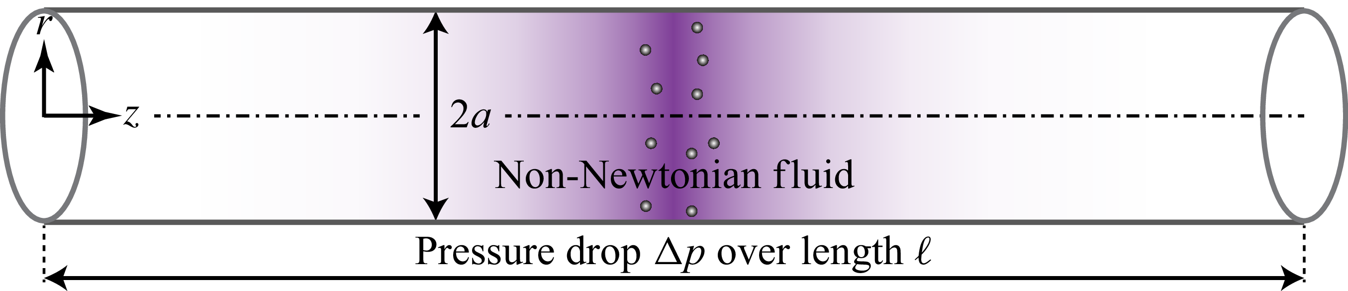
to describe the flow, as shown in figure 1.
$(r,z)$
to describe the flow, as shown in figure 1.
Schematic illustration of the examined configuration for Taylor–Aris dispersion of a complex fluid. The imposed pressure drop $\Delta p$
drives the steady flow of a non-Newtonian fluid through an axisymmetric channel of length
$\Delta p$
drives the steady flow of a non-Newtonian fluid through an axisymmetric channel of length $\ell$
and radius
$\ell$
and radius $a$
. Our interest lies in elucidating the impact of shear-rate-dependent diffusivity on the dispersion of passive tracers in a non-Newtonian flow.
$a$
. Our interest lies in elucidating the impact of shear-rate-dependent diffusivity on the dispersion of passive tracers in a non-Newtonian flow.

Figure 1. Long description
The diagram illustrates a cylindrical channel with a non-Newtonian fluid flowing through it. The channel has a length denoted by the symbol l and a radius denoted by the symbol a. A pressure drop, represented by the symbol Δp, is imposed over the length of the channel, driving the steady flow of the fluid. The diagram includes an axisymmetric representation of the channel, with the z-axis running along the length of the channel and the r-axis representing the radial direction. The fluid flow is depicted with small circles indicating the movement of passive tracers within the fluid. This study aims to elucidate the impact of shear-rate-dependent diffusivity on the dispersion of these tracers in a non-Newtonian flow.
2.1. Derivation of the one-dimensional, cross-sectionally averaged advection–diffusion equation
Here, we begin with the (three-dimensional) advection–diffusion equation, and through an averaging approach, we arrive at a one-dimensional Taylor–Aris description for axial dispersion. Although a shear-rate-dependent viscosity means that the properties of the fluid may vary non-isotropically, we simply use $D$
as a scalar field of the shear rate. Under the assumptions of the azimuthal symmetry and a unidirectional flow in the axial direction,
$D$
as a scalar field of the shear rate. Under the assumptions of the azimuthal symmetry and a unidirectional flow in the axial direction, $\boldsymbol{u}=u(r){\boldsymbol{e}}_z$
, while neglecting the feedback of concentration on the velocity field, the concentration of passive tracers
$\boldsymbol{u}=u(r){\boldsymbol{e}}_z$
, while neglecting the feedback of concentration on the velocity field, the concentration of passive tracers $c(r,z,t)$
evolves according to the advection–diffusion equation
$c(r,z,t)$
evolves according to the advection–diffusion equation
 \begin{equation} \frac {\partial c}{\partial t}+u\frac {\partial c}{\partial z}=\frac {1}{r}\frac {\partial }{\partial r}\left (rD(\dot {\gamma })\frac {\partial c}{\partial r}\right )+\frac {\partial }{\partial z}\left (D(\dot {\gamma })\frac {\partial c}{\partial z}\right )\!, \end{equation}
where $D(\dot {\gamma })$
is the diffusion coefficient of the solute particle that depends on the local shear rate
$D(\dot {\gamma })$
is the diffusion coefficient of the solute particle that depends on the local shear rate $\dot {\gamma }=|\mathrm{d}u(r)/\mathrm{d}r|$
. The governing equation (2.1) is supplemented by the no-flux boundary condition at the channel walls,
$\dot {\gamma }=|\mathrm{d}u(r)/\mathrm{d}r|$
. The governing equation (2.1) is supplemented by the no-flux boundary condition at the channel walls, $\partial c/\partial r=0$
at
$\partial c/\partial r=0$
at $r=a$
.
$r=a$
.
For the Taylor–Aris analysis, we follow the notation of Stone & Brenner (Reference Stone and Brenner1999) (see also Taylor (Reference Taylor1953)) and expand each variable into cross-sectional averages of the form
 \begin{equation} \left \langle (\boldsymbol{\cdot })\right \rangle =\frac {1}{\pi a^{2}}\int _{0}^{a}(\boldsymbol{\cdot })2\pi r\mathrm{d}r=\frac {2}{a^{2}}\int _{0}^{a}(\boldsymbol{\cdot })r\mathrm{d}r, \end{equation}
and deviations from cross-sectionally averaged quantities defined by writing
 \begin{equation} c(r,z,t)=\left \langle c\right \rangle (z,t)+c^\prime(r,z,t)\quad \mathrm{and}\quad u(r)=\left \langle u\right \rangle +u^\prime(r). \end{equation}
Substituting (2.3) into (2.1) yields
 \begin{equation} \frac {\partial \left \langle c\right \rangle }{\partial t}+\frac {\partial c^\prime}{\partial t}+\left \langle u\right \rangle \frac {\partial \left \langle c\right \rangle }{\partial z}+u^\prime\frac {\partial \left \langle c\right \rangle }{\partial z}+\left \langle u\right \rangle \frac {\partial c^\prime}{\partial z}+u^\prime\frac {\partial c^\prime}{\partial z}=\frac {1}{r}\frac {\partial }{\partial r}\left (rD\frac {\partial c^\prime}{\partial r}\right )+D\frac {\partial ^2\left \langle c\right \rangle }{\partial z^2}+D\frac {\partial ^2 c^\prime}{\partial z^2}, \end{equation}
where $D(\dot {\gamma })$
solely depends on the radial coordinate.
$D(\dot {\gamma })$
solely depends on the radial coordinate.
Noting that $\langle \langle c\rangle \rangle =\langle c\rangle$
and
$\langle \langle c\rangle \rangle =\langle c\rangle$
and $\langle c^\prime \rangle = \langle u^\prime \rangle =0$
, we can average (2.4) over the channel cross-section, use the no-flux boundary condition, which, upon averaging, then eliminates the first term after the equal sign, and recognise that
$\langle c^\prime \rangle = \langle u^\prime \rangle =0$
, we can average (2.4) over the channel cross-section, use the no-flux boundary condition, which, upon averaging, then eliminates the first term after the equal sign, and recognise that $\langle D ({\partial ^2\langle c\rangle }/{\partial z^2})\rangle = \langle D\rangle ({\partial ^2\langle c\rangle }/{\partial z^2})$
, which allows us to obtain
$\langle D ({\partial ^2\langle c\rangle }/{\partial z^2})\rangle = \langle D\rangle ({\partial ^2\langle c\rangle }/{\partial z^2})$
, which allows us to obtain
 \begin{equation} \frac {\partial \left \langle c\right \rangle }{\partial t}+\left \langle u\right \rangle \frac {\partial \left \langle c\right \rangle }{\partial z}+\left \langle u^\prime\frac {\partial c^\prime}{\partial z}\right \rangle =\left \langle D\right \rangle \frac {\partial ^2\left \langle c\right \rangle }{\partial z^2}+\left \langle D \frac {\partial ^2 c^\prime}{\partial z^2}\right \rangle \!. \end{equation}
Next, subtracting (2.5) from (2.4), we obtain
 \begin{eqnarray} \frac {\partial c^\prime}{\partial t}&+&u^\prime\frac {\partial \left \langle c\right \rangle }{\partial z}+\left \langle u\right \rangle \frac {\partial c^\prime}{\partial z}+u^\prime\frac {\partial c^\prime}{\partial z}-\left \langle u^\prime\frac {\partial c^\prime}{\partial z}\right \rangle \nonumber \\ &=&\frac {1}{r}\frac {\partial }{\partial r}\left (rD\frac {\partial c^\prime}{\partial r}\right )+\left (D-\left \langle D\right \rangle \right )\frac {\partial ^2\left \langle c\right \rangle }{\partial z^2}+D\frac {\partial ^2 c^\prime}{\partial z^2}-\left \langle D \frac {\partial ^2 c^\prime}{\partial z^2}\right \rangle \!. \end{eqnarray}
Consistent with a Taylor–Aris dispersion analysis, we are interested in the long-time behaviour of cross-stream diffusion, that is, axial distances $\ell \gg \langle u \rangle a^2/D$
, and we consider that
$\ell \gg \langle u \rangle a^2/D$
, and we consider that $|c^\prime|/\langle c \rangle \ll 1$
so that variations of the concentration across the channel are small. Under these assumptions, from an order-of-magnitude analysis, it follows that (2.5) and (2.6) simplify to (see, e.g. Griffiths & Stone Reference Griffiths and Stone2012)
$|c^\prime|/\langle c \rangle \ll 1$
so that variations of the concentration across the channel are small. Under these assumptions, from an order-of-magnitude analysis, it follows that (2.5) and (2.6) simplify to (see, e.g. Griffiths & Stone Reference Griffiths and Stone2012)
 \begin{equation} \frac {\partial \left \langle c\right \rangle }{\partial t}+\left \langle u\right \rangle \frac {\partial \left \langle c\right \rangle }{\partial z} \approx \left \langle D\right \rangle \frac {\partial ^2\left \langle c\right \rangle }{\partial z^2}-\left \langle u^\prime\frac {\partial c^\prime}{\partial z}\right \rangle \!, \end{equation}
and
 \begin{equation} u^\prime\frac {\partial \left \langle c\right \rangle }{\partial z}\approx \frac {1}{r}\frac {\partial }{\partial r}\left (rD(\dot {\gamma })\frac {\partial c^\prime}{\partial r}\right )\!. \end{equation}
The next key step in our analysis is the use of a generalised form of the Stokes–Einstein relation
 \begin{equation} D(\dot {\gamma })=\frac {k_{B}T}{6\pi b\mu (\dot {\gamma })\chi }=\frac { D_0\mu _0}{\mu (\dot {\gamma })}=\frac {D_0}{\mathcal{M}(\dot {\gamma })}\quad \mathrm{with}\quad D_0=\frac {k_{B}T}{6\pi b \mu _0\chi }\,\hbox{and}\, \mathcal{M}=\frac {\mu (\dot {\gamma })}{\mu _{0}}, \end{equation}
where $\mu (\dot {\gamma })$
is the shear-rate-dependent viscosity of the fluid evaluated at the location of the centre of the particle and
$\mu (\dot {\gamma })$
is the shear-rate-dependent viscosity of the fluid evaluated at the location of the centre of the particle and $\mu _{0}$
is the zero-shear-rate viscosity, so that the zero-shear-rate diffusivity
$\mu _{0}$
is the zero-shear-rate viscosity, so that the zero-shear-rate diffusivity $D_0$
is
$D_0$
is $D_0=k_{B}T/(6\pi b \mu _0\chi )$
. Note that we have introduced a constant factor
$D_0=k_{B}T/(6\pi b \mu _0\chi )$
. Note that we have introduced a constant factor $\chi$
as an approximate model to account for the fact that the microscopic problem at the scale of a diffusing object now involves a viscosity field, i.e. the viscosity is a function of position. For the constant viscosity Newtonian limit,
$\chi$
as an approximate model to account for the fact that the microscopic problem at the scale of a diffusing object now involves a viscosity field, i.e. the viscosity is a function of position. For the constant viscosity Newtonian limit, $\mu _0=\mu _N$
, we have
$\mu _0=\mu _N$
, we have $\chi =1$
and
$\chi =1$
and $D_0=D_N$
. For convenience, we have also defined the dimensionless shear-rate-dependent viscosity
$D_0=D_N$
. For convenience, we have also defined the dimensionless shear-rate-dependent viscosity $\mathcal{M}=\mu (\dot {\gamma })/\mu _{0}$
, which is central to the calculation below.
$\mathcal{M}=\mu (\dot {\gamma })/\mu _{0}$
, which is central to the calculation below.
Substituting (2.9) into (2.7) and (2.8), we obtain
 \begin{equation} \frac {\partial \left \langle c\right \rangle }{\partial t}+\left \langle u\right \rangle \frac {\partial \left \langle c\right \rangle }{\partial z} \approx D_0\left \langle \mathcal{M}^{-1}\right \rangle \frac {\partial ^2\left \langle c\right \rangle }{\partial z^2}-\left \langle u^\prime\frac {\partial c^\prime}{\partial z}\right \rangle \!, \end{equation}
and
 \begin{equation} u^\prime\frac {\partial \left \langle c\right \rangle }{\partial z}\approx \frac {D_0}{r}\frac {\partial }{\partial r}\left (r\mathcal{M}^{-1}(\dot {\gamma })\frac {\partial c^\prime}{\partial r}\right )\!. \end{equation}
We remind the reader that, similar to $D(\dot {\gamma })$
, the viscosity
$D(\dot {\gamma })$
, the viscosity $\mathcal{M}(\dot {\gamma })$
solely depends on the radial coordinate
$\mathcal{M}(\dot {\gamma })$
solely depends on the radial coordinate $r$
. Integrating (2.11) once with respect to
$r$
. Integrating (2.11) once with respect to $r$
, while demanding that
$r$
, while demanding that $c^\prime(r,z,t)$
is finite at
$c^\prime(r,z,t)$
is finite at $r=0$
, yields
$r=0$
, yields
 \begin{equation} \frac {\partial c^\prime(r,z,t)}{\partial r}=\frac {1}{D_0}\frac {\partial \left \langle c\right \rangle (z,t) }{\partial z}\frac {\mathrm{d}f(r)}{\mathrm{d}r} \quad \text{with} \quad \frac {\mathrm{d}f(r)}{\mathrm{d}r} =\frac {\mathcal{M}(\dot {\gamma })}{ r}\int _{0}^{r}u^\prime(r^\prime)r^\prime\mathrm{d}r^\prime . \end{equation}
Integrating (2.12) with respect to $r$
, we obtain
$r$
, we obtain
 \begin{equation} c^\prime(r,z,t)=c^\prime(0,z,t)+\frac {1}{D_0}\frac {\partial \left \langle c\right \rangle (z,t)}{\partial z}[f(r)-f(0)], \end{equation}
with
 \begin{equation} f(r)-f(0)=\int _{0}^{r}\frac {\mathcal{M}(\dot {\gamma }(r^\prime))}{r^\prime}\int _{0}^{r^\prime}u^\prime(s)s\mathrm{d}s\mathrm{d}r^\prime, \end{equation}
where $c^\prime(0,z,t)$
can be determined from the requirement that
$c^\prime(0,z,t)$
can be determined from the requirement that $\int _{0}^{a}c^\prime r\mathrm{d}r=0$
, consistent with the definition
$\int _{0}^{a}c^\prime r\mathrm{d}r=0$
, consistent with the definition $\langle c^\prime \rangle =0$
.
$\langle c^\prime \rangle =0$
.
We aim to calculate the final term on the right-hand side of (2.10), which represents the dispersion produced by the coupling of molecular diffusion and the variation of velocity in the cross-section. To this end, we substitute (2.13) into the last term of the right-hand side of (2.10) to obtain
 \begin{equation} \left \langle u^\prime\frac {\partial c^\prime}{\partial z}\right \rangle =\frac {2}{a^{2}D_0}\int _{0}^{a}\left \{ u^\prime(r)r\int _{0}^{r}\left [\frac {\mathcal{M}(\dot {\gamma }(r^\prime))}{r^\prime}\left (\int _{0}^{r^\prime}u^\prime(s)s\mathrm{d}s\right )\right ]\mathrm{d}r^\prime\right \} \mathrm{d}r\frac {\partial ^{2}\left \langle c\right \rangle }{\partial z^{2}}, \end{equation}
where we have used the fact that $\langle u^\prime\partial c^\prime(0,z,t)/\partial z\rangle =0$
.
$\langle u^\prime\partial c^\prime(0,z,t)/\partial z\rangle =0$
.
Integrating by parts and noting that $\langle u^\prime \rangle =\int _{0}^{a}u^\prime(r)r\mathrm{d}r=0$
, (2.14) can be expressed as
$\langle u^\prime \rangle =\int _{0}^{a}u^\prime(r)r\mathrm{d}r=0$
, (2.14) can be expressed as
 \begin{equation} \left \langle u^\prime\frac {\partial c^\prime}{\partial z}\right \rangle =-\frac {2}{a^{2}D_0}\int _{0}^{a}\frac {\mathcal{M}(\dot {\gamma }(r))}{r}\left (\int _{0}^{r}u^\prime(r^\prime)r^\prime\mathrm{d}r^\prime\right )^{2}\mathrm{d}r\frac {\partial ^{2}\left \langle c\right \rangle }{\partial z^{2}}. \end{equation}
Finally, substituting (2.15) into (2.10) and using (2.2), we obtain the following advection–diffusion equation for the evolution of the area-averaged concentration:
 \begin{equation} \frac {\partial \left \langle c\right \rangle }{\partial t}+\left \langle u\right \rangle \frac {\partial \left \langle c\right \rangle }{\partial z}\approx D_{\textit {eff}}\frac {\partial ^{2}\left \langle c\right \rangle }{\partial z^{2}}, \end{equation}
where $D_{\textit {eff}}$
is the effective shear-rate-dependent dispersion coefficient, given as
$D_{\textit {eff}}$
is the effective shear-rate-dependent dispersion coefficient, given as
 \begin{equation} D_{\textit { eff}}=\frac {2D_0}{a^{2}}\left [\int _{0}^{a}\frac {r}{\mathcal{M}(r)}\mathrm{d}r+\frac {1}{D_0^{2}}\int _{0}^{a}\frac {\mathcal{M}(r)}{r}\left (\int _{0}^{r}u^\prime(r^\prime)r^\prime\mathrm{d}r^\prime\right )^{2}\mathrm{d}r\right ]\!, \end{equation}
which has the structure of a traditional Taylor–Aris dispersion analysis.
Scaling by the characteristic dimensions, we introduce the following non-dimensional variables $\tilde {r}=r/a$
,
$\tilde {r}=r/a$
, $\tilde {u}=u/u_c$
,
$\tilde {u}=u/u_c$
, $\tilde {u}^\prime=u^\prime/u_c$
and
$\tilde {u}^\prime=u^\prime/u_c$
and $\mathcal{M}=\mu /\mu _0$
, where
$\mathcal{M}=\mu /\mu _0$
, where $u_c=\Delta p a^2 / (8\mu _0 \ell )$
is the characteristic velocity scale. With this non-dimensionalisation, (2.17) can be expressed in a non-dimensional form as
$u_c=\Delta p a^2 / (8\mu _0 \ell )$
is the characteristic velocity scale. With this non-dimensionalisation, (2.17) can be expressed in a non-dimensional form as
 \begin{equation} \frac {D_{\textit { eff}}}{D_{0}}=\underset {\mathcal{A}}{\underbrace {2\int _{0}^{1}\frac {\tilde {r}}{\mathcal{M}(\tilde {r})}\mathrm{d}\tilde {r}}}+\underset {\mathcal{B}}{\underbrace {2\int _{0}^{1}\frac {\mathcal{M}(\tilde {r})}{\tilde {r}}\left (\int _{0}^{\tilde {r}}\tilde {u}^\prime(\tilde {r}^\prime)\tilde {r}^\prime\mathrm{d}\tilde {r}^\prime\right )^{2}\mathrm{d}\tilde {r}}}\textit{Pe}^{2}=\mathcal{A}+\mathcal{B}\textit{Pe}^2, \end{equation}
where ${\textit{Pe}}=u_c a/D_0=\Delta p a^3 / (8D_0\mu _0 \ell )$
is the Péclet number, and
${\textit{Pe}}=u_c a/D_0=\Delta p a^3 / (8D_0\mu _0 \ell )$
is the Péclet number, and $\mathcal{A}$
and
$\mathcal{A}$
and $\mathcal{B}$
are the non-dimensional coefficients that depend on the fluid rheology.
$\mathcal{B}$
are the non-dimensional coefficients that depend on the fluid rheology.
Equation (2.18) is the main result of this study and highlights several features: (i) in the absence of non-Newtonian effects, the dispersion coefficient results in the classical $\textit{Pe}^2$
scaling, i.e. it varies with the square of the average speed or shear rate. (ii) For a non-Newtonian fluid, when the diffusion coefficient
$\textit{Pe}^2$
scaling, i.e. it varies with the square of the average speed or shear rate. (ii) For a non-Newtonian fluid, when the diffusion coefficient $D$
is independent of shear rate, such that
$D$
is independent of shear rate, such that $\mathcal{M}\equiv 1$
in (2.18), there is a rheological contribution from the integral involving the velocity profile, which has been accounted for in previous studies (see, e.g. Fan & Hwang Reference Fan and Hwang1965; Booras & Krantz Reference Booras and Krantz1976; Sharp Reference Sharp1993; Teodoro et al. Reference Teodoro, Bautista and Méndez2025). (iii) However, the dependence of viscosity and corresponding diffusivity on shear rate clearly indicates that the coefficients
$\mathcal{M}\equiv 1$
in (2.18), there is a rheological contribution from the integral involving the velocity profile, which has been accounted for in previous studies (see, e.g. Fan & Hwang Reference Fan and Hwang1965; Booras & Krantz Reference Booras and Krantz1976; Sharp Reference Sharp1993; Teodoro et al. Reference Teodoro, Bautista and Méndez2025). (iii) However, the dependence of viscosity and corresponding diffusivity on shear rate clearly indicates that the coefficients $\mathcal{A}$
and
$\mathcal{A}$
and $\mathcal{B}$
are influenced by the fluid rheology through the viscosity and velocity profiles. In particular, the coefficient
$\mathcal{B}$
are influenced by the fluid rheology through the viscosity and velocity profiles. In particular, the coefficient $\mathcal{A}$
depends on the viscosity distribution, differing from the value of 1 found in previous studies on Taylor–Aris dispersion analysis in non-Newtonian fluids. Furthermore, the coefficient
$\mathcal{A}$
depends on the viscosity distribution, differing from the value of 1 found in previous studies on Taylor–Aris dispersion analysis in non-Newtonian fluids. Furthermore, the coefficient $\mathcal{B}$
depends on both the viscosity distribution and the deviation from the cross-sectionally averaged velocity profile, in contrast to previous studies that accounted only for the velocity and not for the variation in diffusivity through the viscosity distribution (see, e.g. Sharp Reference Sharp1993; Teodoro et al. Reference Teodoro, Bautista and Méndez2025).
$\mathcal{B}$
depends on both the viscosity distribution and the deviation from the cross-sectionally averaged velocity profile, in contrast to previous studies that accounted only for the velocity and not for the variation in diffusivity through the viscosity distribution (see, e.g. Sharp Reference Sharp1993; Teodoro et al. Reference Teodoro, Bautista and Méndez2025).
We note that for pressure-driven flow of a Newtonian fluid with a constant viscosity $\mu _0=\mu _N$
(
$\mu _0=\mu _N$
( $\mathcal{M}=1$
), we have
$\mathcal{M}=1$
), we have $ \tilde {u}(\tilde {r})=2 (1-\tilde {r}^{2})$
and
$ \tilde {u}(\tilde {r})=2 (1-\tilde {r}^{2})$
and $\tilde {u}^\prime(\tilde {r})=1-2\tilde {r}^{2}$
. Using (2.18), we find that
$\tilde {u}^\prime(\tilde {r})=1-2\tilde {r}^{2}$
. Using (2.18), we find that $D_{\textit { eff}}/D_0=1+\textit{Pe}^2/48$
, as originally found by Taylor (Reference Taylor1953).
$D_{\textit { eff}}/D_0=1+\textit{Pe}^2/48$
, as originally found by Taylor (Reference Taylor1953).
2.2. The cross-sectionally averaged concentration distribution
The cross-sectionally averaged concentration distribution follows from the solution of (2.16), which is a standard advection–diffusion equation with constant coefficients $\langle u\rangle$
and
$\langle u\rangle$
and $D_{\textit {eff}}$
. Nevertheless, we note that, for pressure-driven flow of a non-Newtonian fluid, both
$D_{\textit {eff}}$
. Nevertheless, we note that, for pressure-driven flow of a non-Newtonian fluid, both $\langle u\rangle$
and
$\langle u\rangle$
and $D_{\textit {eff}}$
change depending on the constitutive description. For example, for a given number of passive tracers,
$D_{\textit {eff}}$
change depending on the constitutive description. For example, for a given number of passive tracers, $N_0 = \pi a^2 \int ^{\infty }_{-\infty } \langle c\rangle (z,t)\textrm {d} z$
, injected at time
$N_0 = \pi a^2 \int ^{\infty }_{-\infty } \langle c\rangle (z,t)\textrm {d} z$
, injected at time $t=0$
into the flow at
$t=0$
into the flow at $z=z_0$
, the well-known analytical solution of (2.16) takes the form (Taylor Reference Taylor1953)
$z=z_0$
, the well-known analytical solution of (2.16) takes the form (Taylor Reference Taylor1953)
 \begin{equation} \langle c\rangle (z,t)=\frac {N_{0}}{\pi a^{2}}\frac {1}{\sqrt {4\pi D_{\textit {eff}}t}}\exp \left [-\frac {\left (z-\left (z_{0}+\langle u\rangle t\right )\right )^{2}}{4D_{\textit {eff}}t}\right ]\!, \end{equation}
representing a Gaussian distribution centred at $z_0+\langle u\rangle t$
.
$z_0+\langle u\rangle t$
.
For a Newtonian fluid, $\langle u\rangle =\Delta p a^2 / (8\mu _N \ell )$
and
$\langle u\rangle =\Delta p a^2 / (8\mu _N \ell )$
and $D_{\textit {eff}}/D_N=1+\textit{Pe}^2/48$
. However, for non-Newtonian flows with shear-rate-dependent viscosity, both the average velocity
$D_{\textit {eff}}/D_N=1+\textit{Pe}^2/48$
. However, for non-Newtonian flows with shear-rate-dependent viscosity, both the average velocity $\langle u\rangle$
and the effective dispersion coefficient
$\langle u\rangle$
and the effective dispersion coefficient $D_{\textit {eff}}/D_0= \mathcal{A}+\mathcal{B}\textit{Pe}^2$
change depending on the constitutive description due to the fluid rheology.
$D_{\textit {eff}}/D_0= \mathcal{A}+\mathcal{B}\textit{Pe}^2$
change depending on the constitutive description due to the fluid rheology.
2.3. Remark on a generalised form of the Stokes–Einstein relation
It is well known that, for Newtonian fluids, the diffusivity of a Brownian particle is inversely proportional to the viscosity, as described by the classical Stokes–Einstein relation. However, no such understanding exists for the diffusivity of a particle in non-Newtonian fluid flow with shear-rate-dependent viscosity. Even for the case of diffusion of a colloidal particle of radius $b$
in a polymer solution at rest, the dynamics depends on several length scales, e.g. the monomer or Kuhn length
$b$
in a polymer solution at rest, the dynamics depends on several length scales, e.g. the monomer or Kuhn length $\ell _K$
, a correlation length
$\ell _K$
, a correlation length $\ell _{\textit {cor}}$
, a measure of the entanglement length
$\ell _{\textit {cor}}$
, a measure of the entanglement length $\ell _{\textit {ent}}$
and the radius of gyration of a polymer
$\ell _{\textit {ent}}$
and the radius of gyration of a polymer $\ell _{\textit {rg}}$
. Typically, we expect
$\ell _{\textit {rg}}$
. Typically, we expect $\ell _K\lt \ell _{\textit {cor}}, \ell _{\textit {ent}}\lt \ell _{\textit {rg}}$
. Theory (Brochard-Wyart & de Gennes Reference Brochard-Wyart and de Gennes2000; Cai et al. Reference Cai, Panyukov and Rubinstein2011) and experiments (Kohli & Mukhopadhyay Reference Kohli and Mukhopadhyay2012; Nath et al. Reference Nath, Mangal, Choudhury, Narayanan, Wiesner and Archer2018; Chen et al. Reference Chen, Nikoubashman, Howard, M., Conrad and Palmer2018) show that, for a complex fluid at rest, a Stokes–Einstein-like description of the particle diffusion coefficient is reasonable for
$\ell _K\lt \ell _{\textit {cor}}, \ell _{\textit {ent}}\lt \ell _{\textit {rg}}$
. Theory (Brochard-Wyart & de Gennes Reference Brochard-Wyart and de Gennes2000; Cai et al. Reference Cai, Panyukov and Rubinstein2011) and experiments (Kohli & Mukhopadhyay Reference Kohli and Mukhopadhyay2012; Nath et al. Reference Nath, Mangal, Choudhury, Narayanan, Wiesner and Archer2018; Chen et al. Reference Chen, Nikoubashman, Howard, M., Conrad and Palmer2018) show that, for a complex fluid at rest, a Stokes–Einstein-like description of the particle diffusion coefficient is reasonable for $b\gt \ell _{\textit {rg}}$
, i.e. the diffusion coefficient is expected to be inversely related to the zero-shear-rate viscosity. We note that for small enough solutes the diffusion coefficient is similar, but not equal, to that in the solvent (Cai et al. Reference Cai, Panyukov and Rubinstein2011), in which case we expect the results in the literature with
$b\gt \ell _{\textit {rg}}$
, i.e. the diffusion coefficient is expected to be inversely related to the zero-shear-rate viscosity. We note that for small enough solutes the diffusion coefficient is similar, but not equal, to that in the solvent (Cai et al. Reference Cai, Panyukov and Rubinstein2011), in which case we expect the results in the literature with $D=\text{const.}$
to hold. These remarks support, at least for some systems, the approximate axial dispersion model offered in this work.
$D=\text{const.}$
to hold. These remarks support, at least for some systems, the approximate axial dispersion model offered in this work.
We are not aware of theoretical or experimental studies on how the diffusion coefficient of a colloidal particle varies with shear rate in non-Newtonian flows. Therefore, it is our understanding that the form of the relation between the diffusivity and the shear-rate-dependent viscosity, even in steady non-Newtonian fluid flows, remains an open research question.
As we understand the transport question at the scale of a colloidal (diffusing) particle, for flows as studied in this work, where there are steady viscosity variations, the necessary next steps would be to solve for the analogue of the Stokes–Einstein equation involving the hydrodynamic mobility of the diffusing particle. Some research that has hydrodynamic features of this kind of viscosity-gradient problem has been considered in recent years in the colloid science (Rings et al. Reference Rings, Schachoff, Selmke, Cichos and Kroy2010; Oppenheimer, Navardi & Stone Reference Oppenheimer, Navardi and Stone2016), microrheology (Squires & Mason Reference Squires and Mason2010; Furst & Squires Reference Furst and Squires2017) and active matter communities (Malgaretti, Popescu & Dietrich Reference Malgaretti, Popescu and Dietrich2016; Liebchen et al. Reference Liebchen, Monderkamp, Ten Hagen and Löwen2018; Datt & Elfring Reference Datt and Elfring2019; Esparza López et al. Reference Esparza López, Gonzalez-Gutierrez, Solorio-Ordaz, Lauga and Zenit2021).
3. Illustration of results
To illustrate the use of our main result (2.18), in this section, we calculate the effective shear-rate-dependent dispersion coefficient for a shear-thinning fluid described by the Carreau model and a viscoelastic fluid described by the simplified Phan-Thien–Tanner model.
For a fully developed unidirectional flow in a straight axisymmetric channel, the axial Cauchy momentum equation simplifies to
 \begin{equation} \frac {\mathrm{d}p}{\mathrm{d}z}=-\frac {\Delta p}{\ell }=\frac {1}{r}\frac {\mathrm{d}(r\tau _{\textit {rz}})}{\mathrm{d} r}, \end{equation}
where, for a straight channel, the pressure gradient is constant and can be expressed as $\mathrm{d}p/\mathrm{d}z=-\Delta p/\ell$
. The shear stress component
$\mathrm{d}p/\mathrm{d}z=-\Delta p/\ell$
. The shear stress component $\tau _{\textit {rz}}$
of the deviatoric stress tensor
$\tau _{\textit {rz}}$
of the deviatoric stress tensor $\boldsymbol{\tau }$
entails the description of the non-Newtonian fluid rheology and necessitates the use of a specific constitutive equation for
$\boldsymbol{\tau }$
entails the description of the non-Newtonian fluid rheology and necessitates the use of a specific constitutive equation for $\boldsymbol{\tau }$
(and
$\boldsymbol{\tau }$
(and $\tau _{\textit {rz}}$
). For a given constitutive description, one can find the viscosity
$\tau _{\textit {rz}}$
). For a given constitutive description, one can find the viscosity $\mathcal{M}(\tilde {r})$
and the velocity
$\mathcal{M}(\tilde {r})$
and the velocity $\tilde {u}(\tilde {r})$
required for calculating the dispersion coefficient.
$\tilde {u}(\tilde {r})$
required for calculating the dispersion coefficient.
3.1. Shear thinning: Carreau model
To account for the shear-thinning rheology of the fluid, we consider the Carreau viscosity model for $\mu (\dot {\gamma })$
, which describes three experimentally observed behaviours of viscosity, namely, plateaus in viscosity at very low or very high shear rates and power-law dependence at intermediate shear rates. The constitutive equation for a Carreau viscosity model is (Carreau Reference Carreau1972; Bird et al. Reference Bird, Armstrong and Hassager1987)
$\mu (\dot {\gamma })$
, which describes three experimentally observed behaviours of viscosity, namely, plateaus in viscosity at very low or very high shear rates and power-law dependence at intermediate shear rates. The constitutive equation for a Carreau viscosity model is (Carreau Reference Carreau1972; Bird et al. Reference Bird, Armstrong and Hassager1987)
 \begin{equation} \mu (\dot {\gamma })=\mu _{\infty }+(\mu _{0}-\mu _{\infty })\left (1+(\lambda _C\dot {\gamma })^{2}\right )^{(n-1)/2}, \end{equation}
where $\mu _{0}$
and
$\mu _{0}$
and $\mu _{\infty }$
are the zero- and infinite-shear-rate viscosities, respectively. The power-law index
$\mu _{\infty }$
are the zero- and infinite-shear-rate viscosities, respectively. The power-law index $n$
characterises the degree of shear thinning (
$n$
characterises the degree of shear thinning ( $0\lt n\le 1$
) and
$0\lt n\le 1$
) and $\lambda _C$
is the inverse of a characteristic shear rate at which shear thinning becomes apparent. The case
$\lambda _C$
is the inverse of a characteristic shear rate at which shear thinning becomes apparent. The case $n=1$
,
$n=1$
, $\lambda _C=0$
, or
$\lambda _C=0$
, or $\mu _{0}=\mu _{\infty }$
represents the Newtonian fluid with a constant viscosity
$\mu _{0}=\mu _{\infty }$
represents the Newtonian fluid with a constant viscosity $\mu _{0}$
.
$\mu _{0}$
.
Using the generalised Newtonian model, $\boldsymbol{\tau }=\mu (\dot {\gamma })(\boldsymbol{\nabla }\boldsymbol{u}+(\boldsymbol{\nabla }\boldsymbol{u})^{\mathrm{T}})$
, the axial momentum equation (3.1) takes the form
$\boldsymbol{\tau }=\mu (\dot {\gamma })(\boldsymbol{\nabla }\boldsymbol{u}+(\boldsymbol{\nabla }\boldsymbol{u})^{\mathrm{T}})$
, the axial momentum equation (3.1) takes the form
 \begin{equation} -\frac {\Delta p}{\ell }=\frac {1}{r}\frac {\mathrm{d}}{\mathrm{d}r}\left (r\mu (\dot {\gamma })\frac {\mathrm{d}u}{\mathrm{d}r}\right )\quad \mathrm{with}\quad \dot {\gamma }=-\frac {\mathrm{d} u}{\mathrm{d} r}. \end{equation}
Integrating (3.3) with respect to $r$
and using the regularity of solution at
$r$
and using the regularity of solution at $r=0$
, we obtain
$r=0$
, we obtain
 \begin{equation} -\frac {\Delta p}{\ell }\frac {r}{2}=\mu (\dot {\gamma })\frac {\mathrm{d}u}{\mathrm{d}r}, \end{equation}
so that the shear rate is $\dot {\gamma }=r \Delta p/ (2\mu (\dot {\gamma })\ell )$
. Substituting the latter result into the constitutive equation for the viscosity function results in an implicit nonlinear algebraic equation for
$\dot {\gamma }=r \Delta p/ (2\mu (\dot {\gamma })\ell )$
. Substituting the latter result into the constitutive equation for the viscosity function results in an implicit nonlinear algebraic equation for $\mu$
, which for the Carreau model (3.2) takes the dimensionless form
$\mu$
, which for the Carreau model (3.2) takes the dimensionless form
 \begin{equation} \mathcal{M}=\beta +(1-\beta )\left (1+\left (Cu\tilde {r}\mathcal{M}^{-1}\right )^{2}\right )^{(n-1)/2}, \end{equation}
where $\beta =\mu _{\infty }/\mu _{0}$
,
$\beta =\mu _{\infty }/\mu _{0}$
, $\tilde {r}=r/a$
and
$\tilde {r}=r/a$
and $Cu=\lambda _C\Delta p a/2\mu _{0}\ell$
is the Carreau number based on the pressure drop
$Cu=\lambda _C\Delta p a/2\mu _{0}\ell$
is the Carreau number based on the pressure drop $\Delta p$
(Boyko & Stone Reference Boyko and Stone2021; Zhong et al. Reference Zhong, Mitra, Veilleux, Simmons, Shi and Ardekani2022). For given values of
$\Delta p$
(Boyko & Stone Reference Boyko and Stone2021; Zhong et al. Reference Zhong, Mitra, Veilleux, Simmons, Shi and Ardekani2022). For given values of $Cu, n, \beta$
, we solve numerically (3.5) using MATLAB’s routine fzero to obtain the viscosity distribution
$Cu, n, \beta$
, we solve numerically (3.5) using MATLAB’s routine fzero to obtain the viscosity distribution $\mathcal{M}(\tilde {r})$
.
$\mathcal{M}(\tilde {r})$
.
A summary of the low- $Cu$
, power-law and high-
$Cu$
, power-law and high- $Cu$
asymptotic expressions for
$Cu$
asymptotic expressions for $\mathcal{M}(\tilde {r})$
and
$\mathcal{M}(\tilde {r})$
and $\tilde {u}(\tilde {r})$
, as well as
$\tilde {u}(\tilde {r})$
, as well as $\mathcal{A}$
and
$\mathcal{A}$
and $\mathcal{B}$
appearing in the effective shear-rate-dependent dispersion coefficient (2.18), for the case of a shear-thinning Carreau fluid in an axisymmetric channel. For a description of this flow, see Zhong et al. (Reference Zhong, Mitra, Veilleux, Simmons, Shi and Ardekani2022).
$\mathcal{B}$
appearing in the effective shear-rate-dependent dispersion coefficient (2.18), for the case of a shear-thinning Carreau fluid in an axisymmetric channel. For a description of this flow, see Zhong et al. (Reference Zhong, Mitra, Veilleux, Simmons, Shi and Ardekani2022).

Table 1. Long description
A table with three columns labeled Low-Cu asymptote, Power-law asymptote, and High-Cu asymptote, and four rows labeled with different variables. The table presents mathematical expressions for each variable under different asymptotic conditions. The first row shows expressions for the variable M with values 1, (Cu r raised to the power of (n−1)/n), and beta. The second row shows expressions for the variable u with values 2(1−r^2), a complex expression involving Cu and r, and (2/beta)(1−r^2). The third row shows expressions for the variable A with values 1, a complex expression involving Cu, and 1/beta. The fourth row shows expressions for the variable B with values 1/48, a complex expression involving Cu, and 1/(48 beta).
The effective shear-rate-dependent dispersion coefficient for a shear-thinning Carreau fluid in an axisymmetric channel. ( $a$
) Theoretically predicted value of
$a$
) Theoretically predicted value of $D_{\textit {eff}}/D_0$
as a function of the square of the Péclet number,
$D_{\textit {eff}}/D_0$
as a function of the square of the Péclet number, $\textit{Pe}^2$
, for different values of the Carreau number
$\textit{Pe}^2$
, for different values of the Carreau number $Cu$
. Coefficients (
$Cu$
. Coefficients ( $b$
)
$b$
) $\mathcal{A}$
and (
$\mathcal{A}$
and ( $c$
)
$c$
) $\mathcal{B}$
, defined in (2.18), versus
$\mathcal{B}$
, defined in (2.18), versus $Cu=\lambda _C\Delta p a/2\mu _{0}\ell$
. Dots, crosses and circles represent the semi-analytical results obtained by solving numerically (2.18) using (3.5) and (3.6). Purple solid and cyan dotted lines represent the asymptotic solutions for
$Cu=\lambda _C\Delta p a/2\mu _{0}\ell$
. Dots, crosses and circles represent the semi-analytical results obtained by solving numerically (2.18) using (3.5) and (3.6). Purple solid and cyan dotted lines represent the asymptotic solutions for $Cu\ll 1$
and
$Cu\ll 1$
and $Cu\gg 1$
, respectively. Red dashed lines represent the power-law asymptotic solution for intermediate values of
$Cu\gg 1$
, respectively. Red dashed lines represent the power-law asymptotic solution for intermediate values of $Cu$
. The asymptotic solutions are summarised in table 1. All calculations were performed using
$Cu$
. The asymptotic solutions are summarised in table 1. All calculations were performed using $n=0.4$
and
$n=0.4$
and $\beta =\mu _{\infty }/\mu _{0}=10^{-3}$
.
$\beta =\mu _{\infty }/\mu _{0}=10^{-3}$
.

Figure 2. Long description
The line graph presents the theoretically predicted value of the effective shear-rate-dependent dispersion coefficient as a function of the square of the Peclet number for different values of the Carreau number. The x-axis represents the square of the Peclet number, ranging from 10 to the power of negative 2 to 10 to the power of 4. The y-axis represents the normalized dispersion coefficient, ranging from 10 to the power of 0 to 10 to the power of 6. The graph includes three sets of data points for different Carreau numbers: 2500, 25, and 0.25. Purple solid and cyan dotted lines represent the asymptotic solutions for low and high Carreau numbers, respectively. Red dashed lines represent the power-law asymptotic solution for intermediate values. All values are approximated.
Knowing the viscosity distribution $\mu (r)$
(or
$\mu (r)$
(or $\mathcal{M}(\tilde {r})$
), we can integrate (3.4) again with respect to
$\mathcal{M}(\tilde {r})$
), we can integrate (3.4) again with respect to $r$
and apply the no-slip boundary conditions on the channel walls to obtain the dimensional and corresponding non-dimensional axial velocity
$r$
and apply the no-slip boundary conditions on the channel walls to obtain the dimensional and corresponding non-dimensional axial velocity
 \begin{equation} u(r)=\frac {\Delta p}{2\ell }\int _{r}^{a}\frac {r^\prime}{\mu (r^\prime)}\mathrm{d}r^\prime,\qquad \tilde {u}(\tilde {r})=4\int _{\tilde {r}}^{1}\frac {\tilde {r}^\prime}{\mathcal{M}(\tilde {r}^\prime)}\mathrm{d}\tilde {r}^\prime, \end{equation}
so that $\tilde {u}^\prime(\tilde {r})$
is calculated from (3.6). We present in figure 2(
$\tilde {u}^\prime(\tilde {r})$
is calculated from (3.6). We present in figure 2( $a$
) the dimensionless shear-rate-dependent dispersion coefficient
$a$
) the dimensionless shear-rate-dependent dispersion coefficient $D_{\textit {eff}}/D_0$
as a function of
$D_{\textit {eff}}/D_0$
as a function of $\textit{Pe}^2$
for a shear-thinning Carreau fluid in an axisymmetric channel for different values of
$\textit{Pe}^2$
for a shear-thinning Carreau fluid in an axisymmetric channel for different values of $Cu$
. Dots, crosses and circles represent the semi-analytical results, obtained by solving numerically (2.18) using (3.5) and (3.6). Purple solid, red dashed and cyan dotted lines represent the asymptotic solutions for low, intermediate and high values of
$Cu$
. Dots, crosses and circles represent the semi-analytical results, obtained by solving numerically (2.18) using (3.5) and (3.6). Purple solid, red dashed and cyan dotted lines represent the asymptotic solutions for low, intermediate and high values of $Cu$
, respectively; see table 1. As expected, for a small Carreau number of
$Cu$
, respectively; see table 1. As expected, for a small Carreau number of $Cu = 0.25$
, the viscosity and diffusivity depend only weakly on the shear rate and are approximately constant. As a result, the dispersion coefficient follows the Newtonian-like behaviour (purple curve) originally identified by Taylor (Reference Taylor1953). However, as the Carreau number increases, the dispersion coefficient exceeds the Newtonian value, even at low Péclet numbers. This is due to the shear-thinning effect, which results in a decrease in viscosity and consequently enhances dispersion.
$Cu = 0.25$
, the viscosity and diffusivity depend only weakly on the shear rate and are approximately constant. As a result, the dispersion coefficient follows the Newtonian-like behaviour (purple curve) originally identified by Taylor (Reference Taylor1953). However, as the Carreau number increases, the dispersion coefficient exceeds the Newtonian value, even at low Péclet numbers. This is due to the shear-thinning effect, which results in a decrease in viscosity and consequently enhances dispersion.
Next, we present in figure 2(b,c) the coefficients $\mathcal{A}$
and
$\mathcal{A}$
and $\mathcal{B}$
as a function of
$\mathcal{B}$
as a function of $Cu$
, which depend on the shear-thinning rheology of the Carreau fluid. We observe that both
$Cu$
, which depend on the shear-thinning rheology of the Carreau fluid. We observe that both $\mathcal{A}$
and
$\mathcal{A}$
and $\mathcal{B}$
monotonically increase with
$\mathcal{B}$
monotonically increase with $Cu$
and exceed the values of
$Cu$
and exceed the values of $1$
and
$1$
and $1/48$
, respectively, for
$1/48$
, respectively, for $Cu \geqslant 0.5$
owing to the shear-thinning effect that affects both the viscosity distribution and velocity profile. Furthermore, there is excellent agreement between the semi-analytical results and the asymptotic solutions over the wide range of values of the Carreau number. In particular, the power-law asymptotic solution (red curves) accurately captures the power-law dependence
$Cu \geqslant 0.5$
owing to the shear-thinning effect that affects both the viscosity distribution and velocity profile. Furthermore, there is excellent agreement between the semi-analytical results and the asymptotic solutions over the wide range of values of the Carreau number. In particular, the power-law asymptotic solution (red curves) accurately captures the power-law dependence $Cu^{(1-n)/n}$
of
$Cu^{(1-n)/n}$
of $\mathcal{A}$
and
$\mathcal{A}$
and $\mathcal{B}$
for intermediate shear rates.
$\mathcal{B}$
for intermediate shear rates.
3.2. Viscoelasticity: simplified Phan-Thien–Tanner model
To illustrate these ideas for a viscoelastic rheology, we use the simplified Phan-Thien–Tanner (sPTT) constitutive model (Phan-Thien & Tanner Reference Phan-Thien and Tanner1977; Phan-Thien Reference Phan-Thien1978), which is derived from a Lodge–Yamamoto type of network theory and is widely used to describe the flow of concentrated polymer solutions and melts where there are strong interactions between polymer molecules. Unlike the Oldroyd-B model, which allows polymer chains, represented by elastic dumbbells, to be infinitely extensible, the sPTT model accounts for the finite extensibility of polymer chains and incorporates the shear-thinning effect, similar to the FENE-P model. At steady state, the constitutive equation for the deviatoric stress tensor $\boldsymbol{\tau }$
of the sPTT model takes the form (Phan-Thien & Tanner Reference Phan-Thien and Tanner1977; Phan-Thien Reference Phan-Thien1978)
$\boldsymbol{\tau }$
of the sPTT model takes the form (Phan-Thien & Tanner Reference Phan-Thien and Tanner1977; Phan-Thien Reference Phan-Thien1978)
 \begin{equation} f(\boldsymbol{\tau })\boldsymbol{\tau }+\lambda [\boldsymbol{u}\boldsymbol{\cdot }\boldsymbol{\nabla }\boldsymbol{\tau }-(\boldsymbol{\nabla }\boldsymbol{u})^{\mathrm{T}}\boldsymbol{\cdot }\boldsymbol{\tau }-\boldsymbol{\tau }\boldsymbol{\cdot }(\boldsymbol{\nabla }\boldsymbol{u})]=\mu _0(\boldsymbol{\nabla }\boldsymbol{u}+(\boldsymbol{\nabla }\boldsymbol{u})^{\mathrm{T}}) \quad \mathrm{with}\quad f(\boldsymbol{\tau })=1+\frac {\varepsilon \lambda }{\mu _0} \mathrm{tr}(\boldsymbol{\tau }). \end{equation}
In (3.7), $\lambda$
is the relaxation time,
$\lambda$
is the relaxation time, $\mu _0$
is the viscosity at zero shear rate and
$\mu _0$
is the viscosity at zero shear rate and $ f(\boldsymbol{\tau })$
is a scalar function that linearly depends on the trace of
$ f(\boldsymbol{\tau })$
is a scalar function that linearly depends on the trace of $\boldsymbol{\tau }$
, where
$\boldsymbol{\tau }$
, where $\varepsilon$
is the dimensionless extensibility parameter for the sPTT model. We note that another expression for
$\varepsilon$
is the dimensionless extensibility parameter for the sPTT model. We note that another expression for $f(\boldsymbol{\tau })$
in the Phan-Thien–Tanner (PTT) model has an exponential form,
$f(\boldsymbol{\tau })$
in the Phan-Thien–Tanner (PTT) model has an exponential form, $\exp (\varepsilon \lambda \mathrm{tr}(\boldsymbol{\tau })/\mu _0)$
(Phan-Thien Reference Phan-Thien1978). Nevertheless, as
$\exp (\varepsilon \lambda \mathrm{tr}(\boldsymbol{\tau })/\mu _0)$
(Phan-Thien Reference Phan-Thien1978). Nevertheless, as $\varepsilon$
is generally small, we do not expect significant differences with the results from the linear form of
$\varepsilon$
is generally small, we do not expect significant differences with the results from the linear form of $f(\boldsymbol{\tau })$
.
$f(\boldsymbol{\tau })$
.
Oliveira & Pinho (Reference Oliveira and Pinho1999) analysed the fully developed flow of sPTT fluid, neglecting the solvent contribution, and provided analytical expressions for the velocity, polymer stress components and viscosity distribution in an axisymmetric channel. The fully developed velocity profile of the sPTT fluid can be expressed as (Oliveira & Pinho Reference Oliveira and Pinho1999)
 \begin{equation} u(r)=\frac {\Delta pa^{2}}{4\mu _{0}\ell }\left (1-\frac {r^{2}}{a^{2}}\right )\left [1+\frac {\varepsilon \lambda ^{2}(\Delta p)^{2}a^{2}}{4\mu _{0}^{2}\ell ^{2}}\left (1+\frac {r^{2}}{a^{2}}\right )\right ]\!, \end{equation}
so that the corresponding non-dimensional form of the axial velocity is
 \begin{equation} \tilde {u}(\tilde {r})=2(1-\tilde {r}^{2})\left [1+16\varepsilon {\textit{Wi}}^{2}(1+\tilde {r}^{2})\right ]\!, \end{equation}
where $\textit{Wi}=\lambda u_c /a$
is the Weissenberg number, which is the product of the relaxation time of the fluid,
$\textit{Wi}=\lambda u_c /a$
is the Weissenberg number, which is the product of the relaxation time of the fluid, $\lambda$
, and the characteristic shear rate of the flow,
$\lambda$
, and the characteristic shear rate of the flow, $u_c/a$
. We note that
$u_c/a$
. We note that $\tilde {u}^\prime(\tilde {r})$
can be calculated from (3.9).
$\tilde {u}^\prime(\tilde {r})$
can be calculated from (3.9).
The corresponding dimensional and non-dimensional viscosity distributions in our notation are (Oliveira & Pinho Reference Oliveira and Pinho1999)
 \begin{equation} \frac {\mu (r)}{\mu _{0}}=\left (1+\frac {\varepsilon \lambda ^{2}(\Delta p)^{2}r^{2}}{2\mu _{0}^{2}\ell ^{2}}\right )^{-1}, \qquad \mathcal{M}(\tilde {r})=\frac {1}{1+32\varepsilon {\textit{Wi}}^{2}\tilde {r}^{2}}. \end{equation}
Using (2.18) and (3.9)–(3.10), we obtain closed-form analytical expressions for the coefficients $\mathcal{A}$
and
$\mathcal{A}$
and $\mathcal{B}$
in the case of the sPTT model
$\mathcal{B}$
in the case of the sPTT model
 \begin{equation} \mathcal{A}=1 + 16 \varepsilon {\textit{Wi}}^{2}, \end{equation}
 \begin{eqnarray} \mathcal{B}&=&\frac {16 \varepsilon {\textit{Wi}}^2 (16 \varepsilon {\textit{Wi}}^2 (8 \varepsilon {\textit{Wi}}^2 (195+1024 \varepsilon {\textit{Wi}}^2)+125)+75)+15}{4423680 \varepsilon ^3 {\textit{Wi}}^6} \nonumber \\[5pt] &&-\frac {(1+48 \varepsilon {\textit{Wi}}^2+512 \varepsilon ^2 {\textit{Wi}}^4)^2 \ln (1+32 \varepsilon {\textit{Wi}}^2)}{9437184 \varepsilon ^4 {\textit{Wi}}^8}. \end{eqnarray}
We have verified that as $\varepsilon {\textit{Wi}}^2$
approaches zero, the value of
$\varepsilon {\textit{Wi}}^2$
approaches zero, the value of $\mathcal{B}$
approaches the Newtonian limit of
$\mathcal{B}$
approaches the Newtonian limit of $1/48$
. We note that the non-dimensional viscosity and velocity, as well as
$1/48$
. We note that the non-dimensional viscosity and velocity, as well as $\mathcal{A}$
and
$\mathcal{A}$
and $\mathcal{B}$
, (3.11), depend solely on the single dimensionless parameter
$\mathcal{B}$
, (3.11), depend solely on the single dimensionless parameter $\varepsilon {\textit{Wi}}^2$
. Therefore, we present our results as a function of
$\varepsilon {\textit{Wi}}^2$
. Therefore, we present our results as a function of $\varepsilon ^{1/2}\textit{Wi}$
, which we refer to as the modified Weissenberg number.
$\varepsilon ^{1/2}\textit{Wi}$
, which we refer to as the modified Weissenberg number.
We present in figure 3( $a$
) the dimensionless shear-rate-dependent dispersion coefficient
$a$
) the dimensionless shear-rate-dependent dispersion coefficient $D_{\textit {eff}}/D_0$
as a function of
$D_{\textit {eff}}/D_0$
as a function of $\textit{Pe}^2$
for a viscoelastic Phan-Thien–Tanner fluid in an axisymmetric channel for different values of
$\textit{Pe}^2$
for a viscoelastic Phan-Thien–Tanner fluid in an axisymmetric channel for different values of $\varepsilon ^{1/2}\textit{Wi}$
. Dots, crosses and circles represent the analytical results (3.11). Purple solid and cyan dotted lines represent the asymptotic solutions for low and high values of
$\varepsilon ^{1/2}\textit{Wi}$
. Dots, crosses and circles represent the analytical results (3.11). Purple solid and cyan dotted lines represent the asymptotic solutions for low and high values of $\varepsilon ^{1/2}\textit{Wi}$
, respectively, summarised in table 2. Similar to the Carreau fluid, when
$\varepsilon ^{1/2}\textit{Wi}$
, respectively, summarised in table 2. Similar to the Carreau fluid, when $\varepsilon ^{1/2}\textit{Wi}$
is low (e.g.
$\varepsilon ^{1/2}\textit{Wi}$
is low (e.g. $\varepsilon ^{1/2}\textit{Wi}= 0.05$
), the dispersion coefficient in the sPTT fluid exhibits Newtonian-like behaviour (purple curve). However, as the modified Weissenberg number increases, the dispersion coefficient surpasses the Newtonian value for all values of Péclet numbers due to enhanced shear-thinning behaviour.
$\varepsilon ^{1/2}\textit{Wi}= 0.05$
), the dispersion coefficient in the sPTT fluid exhibits Newtonian-like behaviour (purple curve). However, as the modified Weissenberg number increases, the dispersion coefficient surpasses the Newtonian value for all values of Péclet numbers due to enhanced shear-thinning behaviour.
A summary of the low- and high- $\varepsilon ^{1/2}\textit{Wi}$
asymptotic expressions for
$\varepsilon ^{1/2}\textit{Wi}$
asymptotic expressions for $\mathcal{M}(\tilde {r})$
and
$\mathcal{M}(\tilde {r})$
and $\tilde {u}(\tilde {r})$
, as well as
$\tilde {u}(\tilde {r})$
, as well as $\mathcal{A}$
and
$\mathcal{A}$
and $\mathcal{B}$
appearing in the effective shear-rate-dependent dispersion coefficient (2.18), for the case of a viscoelastic Phan-Thien–Tanner fluid in an axisymmetric channel. The results for these two distinguished limits follow in a straightforward way from (3.9)–(3.11).
$\mathcal{B}$
appearing in the effective shear-rate-dependent dispersion coefficient (2.18), for the case of a viscoelastic Phan-Thien–Tanner fluid in an axisymmetric channel. The results for these two distinguished limits follow in a straightforward way from (3.9)–(3.11).

Table 2. Long description
The table presents asymptotic expressions for the effective shear-rate-dependent dispersion coefficient of a viscoelastic PTT fluid in an axisymmetric channel. It includes expressions for the low and high Weissenberg number asymptotes. The table has four rows and three columns, with the first column listing the variables, the second column showing the low-epsilon to the power of one-half Weissenberg number asymptote, and the third column showing the high-epsilon to the power of negative one-half Weissenberg number asymptote. The variables include M, u-tilde, A, and B, each with corresponding expressions for the two asymptotes.
The effective shear-rate-dependent dispersion coefficient for a viscoelastic Phan-Thien–Tanner fluid in an axisymmetric channel. ( $a$
) Theoretically predicted value of
$a$
) Theoretically predicted value of $D_{\textit {eff}}/D_0$
as a function of the square of the Péclet number,
$D_{\textit {eff}}/D_0$
as a function of the square of the Péclet number, $\textit{Pe}^2$
, for different values of
$\textit{Pe}^2$
, for different values of $\varepsilon ^{1/2}\textit{Wi}$
. Coefficients (
$\varepsilon ^{1/2}\textit{Wi}$
. Coefficients ( $b$
)
$b$
) $\mathcal{A}$
and (
$\mathcal{A}$
and ( $c$
)
$c$
) $\mathcal{B}$
, defined in (2.18), versus
$\mathcal{B}$
, defined in (2.18), versus $\varepsilon ^{1/2}\textit{Wi}=\varepsilon ^{1/2}\lambda \Delta p a/8\mu _{0}\ell$
. Dots, crosses and circles represent the analytical results (3.11). Purple solid and cyan dotted lines represent the asymptotic solutions for
$\varepsilon ^{1/2}\textit{Wi}=\varepsilon ^{1/2}\lambda \Delta p a/8\mu _{0}\ell$
. Dots, crosses and circles represent the analytical results (3.11). Purple solid and cyan dotted lines represent the asymptotic solutions for $\varepsilon ^{1/2}\textit{Wi}\ll 1$
and
$\varepsilon ^{1/2}\textit{Wi}\ll 1$
and $\varepsilon ^{1/2}\textit{Wi}\gg 1$
, respectively. The asymptotic solutions are summarised in table 2.
$\varepsilon ^{1/2}\textit{Wi}\gg 1$
, respectively. The asymptotic solutions are summarised in table 2.

Figure 3. Long description
The line graph presents the theoretically predicted value of the effective dispersion coefficient as a function of the square of the Peclet number for different values of epsilon to the power of one half times the Weissenberg number. The x-axis represents the square of the Peclet number, ranging from 10 to the power of negative 2 to 10 to the power of 4. The y-axis represents the effective dispersion coefficient normalized by the initial diffusion constant, ranging from 10 to the power of 0 to 10 to the power of 6. The graph includes three data sets for different values of epsilon to the power of one half times the Weissenberg number: 0.05, 0.5, and 5. Each data set is represented by different symbols: circles for 5, diamonds for 0.5, and crosses for 0.05. Additionally, the graph includes asymptotic solutions for low and high values of epsilon to the power of one half times the Weissenberg number, represented by purple solid and cyan dotted lines, respectively. The asymptotic solutions are summarized in table 2. All values are approximated.
In addition, we show in figure 3(b,c) the coefficients $\mathcal{A}$
and
$\mathcal{A}$
and $\mathcal{B}$
as a function of
$\mathcal{B}$
as a function of $\varepsilon ^{1/2}\textit{Wi}$
, which depend on the rheology of the sPTT fluid. Similar to the behaviour of a Carreau fluid, the shear-thinning effect in the sPTT model modifies both the viscosity distribution and the velocity profile, resulting in a monotonic increase in
$\varepsilon ^{1/2}\textit{Wi}$
, which depend on the rheology of the sPTT fluid. Similar to the behaviour of a Carreau fluid, the shear-thinning effect in the sPTT model modifies both the viscosity distribution and the velocity profile, resulting in a monotonic increase in $\mathcal{A}$
and
$\mathcal{A}$
and $\mathcal{B}$
with
$\mathcal{B}$
with $\varepsilon ^{1/2}\textit{Wi}$
. We observe excellent agreement between our analytical predictions (3.11) and the asymptotic results. In particular, the high-
$\varepsilon ^{1/2}\textit{Wi}$
. We observe excellent agreement between our analytical predictions (3.11) and the asymptotic results. In particular, the high- $\varepsilon ^{1/2}\textit{Wi}$
asymptotic solutions provide an accurate description of both
$\varepsilon ^{1/2}\textit{Wi}$
asymptotic solutions provide an accurate description of both $\mathcal{A}$
and
$\mathcal{A}$
and $\mathcal{B}$
even at
$\mathcal{B}$
even at $\varepsilon ^{1/2}\textit{Wi}=1$
, demonstrating their wide range of applicability.
$\varepsilon ^{1/2}\textit{Wi}=1$
, demonstrating their wide range of applicability.
4. Concluding remarks
In this work, we have reconsidered Taylor–Aris dispersion in pressure-driven flows of complex fluids and explicitly recognised the dependence of the diffusivity on the shear rate and the shear-rate-dependent viscosity, via an approximate Stokes–Einstein-like description; see § 2.3 for a discussion of this approximation and its limitations. In particular, based on our calculation, the general form of the dimensionless dispersion coefficient (2.18) has the expected Péclet number squared dependence, with two coefficients $\mathcal{A}$
and
$\mathcal{A}$
and $\mathcal{B}$
that are dependent on the rheology of the complex fluid. Previous literature all had
$\mathcal{B}$
that are dependent on the rheology of the complex fluid. Previous literature all had $\mathcal{A}=1$
with a rheology-dependent coefficient
$\mathcal{A}=1$
with a rheology-dependent coefficient $\mathcal{B}$
, though the latter also did not incorporate a shear-rate-dependent diffusivity. We have illustrated the use of our approach by considering steady flows of a shear-thinning Carreau fluid and a viscoelastic Phan-Thien–Tanner fluid and calculating their effective shear-rate-dependent axial dispersion coefficients.
$\mathcal{B}$
, though the latter also did not incorporate a shear-rate-dependent diffusivity. We have illustrated the use of our approach by considering steady flows of a shear-thinning Carreau fluid and a viscoelastic Phan-Thien–Tanner fluid and calculating their effective shear-rate-dependent axial dispersion coefficients.
Finally, we note that Taylor–Aris dispersion analysis in pressure-driven flows of shear-rate-dependent fluids may be further complicated when one accounts for the non-isotropic nature of the fluid properties. To recognise some of the complexities that arise for the general problem, consider the case in this work of steady channel flows that involve viscosity variations with shear rate, i.e. the viscosity is a scalar field of position. However, the corresponding diffusivity may take the form of a second-order tensor field, since the resistance to a motion of a sphere (or the force–velocity relation) will be different for motions along as compared with transverse to the viscosity gradient. This detail would then enter the advection–diffusion (2.1) and subsequent steps. For example, the components $D_{\textit {rr}}$
and
$D_{\textit {rr}}$
and $D_{\textit {zz}}$
, respectively, would enter the radial and axial diffusive terms, which, in the simplest case, would influence results as
$D_{\textit {zz}}$
, respectively, would enter the radial and axial diffusive terms, which, in the simplest case, would influence results as $\mathcal{A}$
would then involve
$\mathcal{A}$
would then involve $D_{\textit {zz}}$
and
$D_{\textit {zz}}$
and $\mathcal{B}$
would involve
$\mathcal{B}$
would involve $D_{\textit {rr}}$
. Clearly, there are significant theoretical questions to think about to better characterise dispersion in the flows of complex fluids.
$D_{\textit {rr}}$
. Clearly, there are significant theoretical questions to think about to better characterise dispersion in the flows of complex fluids.
Acknowledgements
We thank J. C. Conrad for a helpful discussion on colloidal diffusion in polymer solutions.
Funding
E.B. acknowledges the support by grant no. 2022688 from the US-Israel Binational Science Foundation (BSF) and the Israeli Council for Higher Education Yigal Alon Fellowship. H.A.S. acknowledges the support from grant no. CBET-2246791 from the United States National Science Foundation (NSF).
Declaration of interests
The authors report no conflict of interest.
 Δp
Δp ℓ
ℓ a
a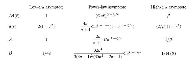
 Cu
Cu Cu
Cu M(r~)
M(r~) u~(r~)
 A
A B
B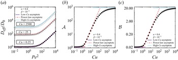
 a
a Deff/D0
 Pe2
Pe2 Cu
Cu b
b A
A c
c B
B Cu=λCΔpa/2μ0ℓ
 Cu≪1
Cu≪1 Cu≫1
Cu≫1 Cu
Cu n=0.4
n=0.4 β=μ∞/μ0=10−3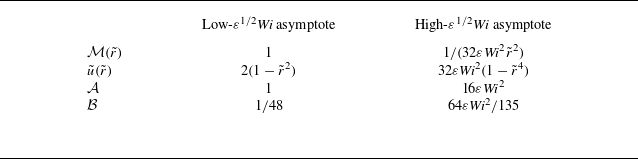
 ε1/2Wi
 M(r~)
M(r~) u~(r~)
 A
A B
B
 a
a Deff/D0
 Pe2
Pe2 ε1/2Wi
 b
b A
A c
c B
B ε1/2Wi=ε1/2λΔpa/8μ0ℓ
 ε1/2Wi≪1
 ε1/2Wi≫1
 Open access

