


1. Introduction
Vortex-induced vibration (VIV) of circular cylinders has been investigated extensively. When an elastically mounted rigid circular cylinder is placed in a fluid flow, there is a lock-in phenomenon where the vortex shedding frequency synchronises with the vibration frequency, instead of following the Strouhal law (Williamson & Govardhan Reference Williamson and Govardhan2004, Reference Williamson and Govardhan2008; Zhao Reference Zhao2023). Many structures, such as floating platforms in the ocean, the decks of suspended bridges, and icy powerlines, are prone to torsional vibration, which is a recipe for structural failure. Compared with VIV in the crossflow direction, very limited studies have been conducted to investigate rotational vibration of cylinders in flow. Zhu et al. (Reference Zhu, Zhao, Qiu, Lin, Du and Dong2023) investigated three-degrees-of-freedom VIV of two rigidly coupled circular cylinders in inline, crossflow and rotational directions, and reported that the rotational vibration widened the lock-in range. Sun et al. (Reference Sun, Zhang, Tao, Han and Xiao2023) simulated rotational VIV of an eccentric circular cylinder at Re = 100. The effects of the distance between the rotational centre and the cylinder's axis on the vibration were examined under various mass ratios. Like the translational vibration case, lock-in occurs when the vortex shedding frequency is close to the rotational natural frequency. The maximum rotational angle is found to be 36.3° in the lock-in range. The wake was always in a 2S mode; the alignment of the vortices in the wake is affected by the response mode. Xu et al. (Reference Xu, Ying, Li and Zhang2016) conducted experiments on flow-induced tortional vibration of a bridge deck. They found a distinct lock regime of VIV with maximum angular displacement 1.5°.
In the above-mentioned studies of vortex-induced torsional/rotational vibration, the maximum angular displacement is small (less than 40°). Galloping is a typical response mode of a non-circular object in fluid flow. If a non-circular object is supported by a very soft torsional spring, and the flow-induced moment around the rotation axis is strong, then there is potential for galloping in the torsional direction. In this study, torsional flow-induced vibration of a two-dimensional equilateral triangular prism (TP) is investigated to identify galloping and find the correlation between the flow velocity and the angular vibration amplitude. Under the fluid-induced moment, the TP that is elastically supported by a torsional spring undergoes torsional vibration as shown in figure 1(a). A reference position is defined as the position where one vertex of the prism faces the flow. Two rotational angles are defined: (i) the rotational angle γ that is relative to the reference position; and (ii) the torsional displacement $\theta$
that is relative to the initial angle at the static balance position of the TP, which has angular displacement γ
0 relative to the reference position, also referred to as the angle of attack. The relation between the torsional displacement
$\theta$
that is relative to the initial angle at the static balance position of the TP, which has angular displacement γ
0 relative to the reference position, also referred to as the angle of attack. The relation between the torsional displacement $\theta$
and the rotational angle γ is
$\theta$
and the rotational angle γ is $\theta =\gamma -\gamma _{0}$
. Torsional vibration of the TP at three initial angles is studied (as shown in figures 1
c–e). In cases A, B and C, γ
0 = 0, π/3 and π/6, respectively. Under the static balance position, one vertex of the prism faces the incoming flow in case A, and one boundary faces the incoming flow in case B. The natural frequency measured in vacuum of the elastically supported cylinder in the rotational directions is f
n
, and the reduced velocity is defined as
$\theta =\gamma -\gamma _{0}$
. Torsional vibration of the TP at three initial angles is studied (as shown in figures 1
c–e). In cases A, B and C, γ
0 = 0, π/3 and π/6, respectively. Under the static balance position, one vertex of the prism faces the incoming flow in case A, and one boundary faces the incoming flow in case B. The natural frequency measured in vacuum of the elastically supported cylinder in the rotational directions is f
n
, and the reduced velocity is defined as $V_{r}=U/(f_{n}b)$
, where U is the velocity of the incoming flow, and b is the side length of the cross-section (equal to one-third of the perimeter). A Cartesian coordinate system is defined with its origin at the centre of the TP, and x- and y-directions in the inline and crossflow directions of the incoming flow, respectively.
$V_{r}=U/(f_{n}b)$
, where U is the velocity of the incoming flow, and b is the side length of the cross-section (equal to one-third of the perimeter). A Cartesian coordinate system is defined with its origin at the centre of the TP, and x- and y-directions in the inline and crossflow directions of the incoming flow, respectively.
Sketch of torsional vibration of flow past an elastically supported equilateral TP: (a) definition of the rotation angle γ and rotation displacement θ; (b) computational domain; (c) case A, with $\gamma _{0}=0$
(vertex faces the flow); (d) case B, with with
$\gamma _{0}=0$
(vertex faces the flow); (d) case B, with with $\gamma _{0}={\pi }/{3}$
(one side boundary faces the flow); (e) case C, with
$\gamma _{0}={\pi }/{3}$
(one side boundary faces the flow); (e) case C, with $\gamma _{0}={\pi }/{6}$
.
$\gamma _{0}={\pi }/{6}$
.

The Reynolds number is defined as Re = Ub/ν, where ν is the kinematic viscosity of the fluid, and the mass ratio is defined as m * = m/md , where m and md are the masses of the TP and displaced fluid, respectively. In this study, Re = 150 and m * = 2.5 remain constant.
2. Numerical method
The two-dimensional incompressible Navier–Stokes (NS) equations are the governing equations for simulating the flow. The non-dimensional coordinates, velocity, time and pressure are defined as $x_{{i}}=\hat{x}_{{i}}/b$
,
$x_{{i}}=\hat{x}_{{i}}/b$
, $u_{{i}}=\hat{u}_{{i}}/U$
,
$u_{{i}}=\hat{u}_{{i}}/U$
, $t=\hat{t}U/b$
and
$t=\hat{t}U/b$
and $p=\hat{p}/(\rho U^{2})$
, respectively, where variables with and without a hat stand for dimensional and non-dimensional variables, respectively, ρ is the density of the fluid, x
1 = x, x
2 = y are the coordinates, ui
is the velocity in the xi
-direction, t is the time, and p is the pressure. The arbitrary Lagrangian–Eulerian (ALE) scheme is employed in the numerical model to cope with the moving boundary of the TP. Considering the effect of the mesh movement in the ALE scheme, the non-dimensional NS equations are
$p=\hat{p}/(\rho U^{2})$
, respectively, where variables with and without a hat stand for dimensional and non-dimensional variables, respectively, ρ is the density of the fluid, x
1 = x, x
2 = y are the coordinates, ui
is the velocity in the xi
-direction, t is the time, and p is the pressure. The arbitrary Lagrangian–Eulerian (ALE) scheme is employed in the numerical model to cope with the moving boundary of the TP. Considering the effect of the mesh movement in the ALE scheme, the non-dimensional NS equations are
 \begin{equation}\frac{{\partial {u_i}}}{{\partial t}} + ( {{u_{\!j}} - {u_{j,\textit{mesh}}}})\frac{{\partial {u_i}}}{{\partial {x_{\!j}}}} + \frac{{\partial p}}{{\partial {x_i}}} = \frac{1}{{\textit{Re} }}\frac{{{\partial ^2}{u_i}}}{{\partial {x_{\!j}}\,\partial {x_{\!j}}}},\end{equation}
 \begin{equation}\frac{{\partial {u_i}}}{{\partial {x_i}}} = 0,\end{equation}
where u j,mesh is the velocity of the mesh movement. In the ALE scheme, the mesh nodes move according to the new position of the TP. Rotating the surface of the cylinder with a velocity the same as the flow velocity would make the mesh so distorted that calculation cannot be continued. To avoid this, the computational domain is divided into a circular inner zone that rotates together with the cylinder and a stationary outer zone, as shown in figure 1(b). The continuity of velocity and pressure is ensured in the very thin overlapping layer between rotating inner zone and stationary outer zone.
The non-dimensional equation of motion of the cylinder in rotational directions is
 \begin{equation}\ddot{\theta }+\frac{4\pi \mathit{\zeta }_{\theta}}{V_{r}}\dot{\theta }+\frac{4\pi ^{2}}{{V}_{r}^{2}}\theta =\frac{C_{\!{M}}}{2J_{r}},\end{equation}
where $\ddot{\theta }$
,
$\ddot{\theta }$
, $\dot{\theta }$
and θ are non-dimensional rotational acceleration, velocity and displacement in the θ-direction, respectively,
$\dot{\theta }$
and θ are non-dimensional rotational acceleration, velocity and displacement in the θ-direction, respectively, $J_{r}=J/(\rho b^{4})$
is the non-dimensional mass moment of inertia,
$J_{r}=J/(\rho b^{4})$
is the non-dimensional mass moment of inertia, $C_{M}=2M/(\rho b^{2}U^{2})$
is the moment coefficient, M is the fluid moment around the rotation centre, and
$C_{M}=2M/(\rho b^{2}U^{2})$
is the moment coefficient, M is the fluid moment around the rotation centre, and $\mathit{\zeta }_{\theta}$
is the damping ratio in the rotational direction, which is set to zero in this study to achieve the maximum vibration angle. The cross-sectional area and the mass moment of inertia of a homogeneous equilateral TP are
$\mathit{\zeta }_{\theta}$
is the damping ratio in the rotational direction, which is set to zero in this study to achieve the maximum vibration angle. The cross-sectional area and the mass moment of inertia of a homogeneous equilateral TP are $A=\sqrt{3}\,b^{2}/4$
and
$A=\sqrt{3}\,b^{2}/4$
and $J=\rho b^{2}A/12$
, respectively.
$J=\rho b^{2}A/12$
, respectively.
The numerical method for solving the NS equations is the Petrov–Galerkin finite element method (PG-FEM) developed by Zhao et al. (Reference Zhao, Cheng, Teng and Dong2007), which has been proved capable of accurately simulating translational flow-induced vibrations of rotating and non-rotating cylinders (Zhao & Cheng Reference Zhao and Cheng2011; Zhao Reference Zhao2013; Zhao, Zhang & Liu Reference Zhao, Zhang and Liu2025). In all the simulations, the non-dimensional size of the outer zone in figure 1(b) is 100 in the streamwise direction, and 100 in the crossflow direction, corresponding to blockage ratio 0.01. The TP is located at the centre in the crossflow direction, and 20 from the inlet boundary. Figure 2 shows the computational mesh for case B. The non-dimensional inner and outer radii of the annular overlapping layer between the two zones are 1.2 and 1.235, respectively. The whole computational domain is divided into 170 171 four-node linear quadrilateral elements. The non-dimensional element size next to the surface of the prism is 0.0021. The maximum wall unit defined as $y^{+}=u_{f}y_{1}/\nu$
ranges between 1.1 and 1.3 in all the simulations, where
$y^{+}=u_{f}y_{1}/\nu$
ranges between 1.1 and 1.3 in all the simulations, where $u_{f}=\sqrt{\tau /\rho }$
is the friction velocity,
$u_{f}=\sqrt{\tau /\rho }$
is the friction velocity, $y_{1}$
is the distance between the wall and the first layer nodes next to the wall, and
$y_{1}$
is the distance between the wall and the first layer nodes next to the wall, and $\tau$
is the shear stress along the surface of the prism. This maximum
$\tau$
is the shear stress along the surface of the prism. This maximum $y^{+}$
occurs near one of the vortices of the prism, where the fluid velocity is very high. The value of
$y^{+}$
occurs near one of the vortices of the prism, where the fluid velocity is very high. The value of $y^{+}$
on other places along the prism surface is generally smaller than 0.5.
$y^{+}$
on other places along the prism surface is generally smaller than 0.5.
Computational mesh for case B. The area within the two red circles is the overlapping layer. (a) Mesh near the prism. (b) Mesh near a vertex.

3. Mesh-dependency study and validation
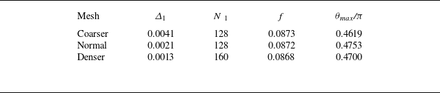
In the mesh-dependency study, simulation for V r = 8 in case A is repeated using two meshes that are coarser and denser than the computational mesh shown in figure 2. A reduced velocity of 8 is chosen because it has ideally periodic vibration that enables quantitative comparison between the results from the two meshes. Because the angular speed of the vibration does not increase when the reduced velocity further increases, the mesh dependency study at this reduced velocity is adequate to ensure that the mesh is sufficiently dense for all the simulated cases. In table 1, Δ 1 and n 1 represent the first-layer mesh size next to the wall in the direction perpendicular to the wall, and the finite element number along each boundary of the TP, respectively. The vibration becomes periodic after t = 200 for all the meshes, as shown in figure 3. The difference between the vibration amplitudes of the denser and normal meshes is 1.11 %.
Vibration frequency and amplitude from three meshes at V r = 8 in case A.

Time histories of the vibration displacement at V r = 8 in case A.

As there are no available data of purely torsional vibration, VIV of an elliptic cylinder in both transverse and rotational directions is simulated, and results are compared with Wang, Zhai & Chen (Reference Wang, Zhai and Chen2019) for validation. Figure 4(a) is a sketch of the elastically supported elliptic cylinder that can vibrate in both the rotational and crossflow directions. The equivalent diameter of the elliptic cylinder is defined as $D=2\sqrt{ab}$
, where a and b are the minor and major radii of the cylinder, respectively, the cross-sectional area is
$D=2\sqrt{ab}$
, where a and b are the minor and major radii of the cylinder, respectively, the cross-sectional area is $A=\pi ab$
, the reduced mass is
$A=\pi ab$
, the reduced mass is $M_{r}=m/(\rho D^{2})=10$
, corresponding to mass ratio
$M_{r}=m/(\rho D^{2})=10$
, corresponding to mass ratio $m^{*}=m/(\rho A)=12.732$
, and the non-dimensional moment of inertia is
$m^{*}=m/(\rho A)=12.732$
, and the non-dimensional moment of inertia is $J_{r}=J/(\rho D^{4})=M_{r}(a^{2}+b^{2})/(4D^{2})$
for a homogeneous cylinder. The Reynolds number based on the equivalent diameter is
$J_{r}=J/(\rho D^{4})=M_{r}(a^{2}+b^{2})/(4D^{2})$
for a homogeneous cylinder. The Reynolds number based on the equivalent diameter is $\textit{Re}=({UD}/{\nu })=150$
, the translational and rotational vibrations have the same natural frequency
$\textit{Re}=({UD}/{\nu })=150$
, the translational and rotational vibrations have the same natural frequency $f_{ny}=f_{n\theta }=f_{n}$
, and the damping ratios in the y- and θ-directions are the same:
$f_{ny}=f_{n\theta }=f_{n}$
, and the damping ratios in the y- and θ-directions are the same: $\zeta _{y}=\zeta _{\theta }=0.003$
.
$\zeta _{y}=\zeta _{\theta }=0.003$
.
In addition to solving (2.3) for torsional vibration, the following translational equation of motion is solved to calculate the vibration in the y-direction:
 \begin{equation}\ddot{Y}+\frac{4\pi {\zeta }_{{y}}}{V_{r}}\dot{Y}+\frac{4\pi ^{2}}{{V}_{r}^{2}}Y=\frac{2C_{\!{L}}}{\pi m^{*}},\end{equation}
where $\ddot{Y}$
,
$\ddot{Y}$
, $\dot{Y}$
and Y are the non-dimensional acceleration, velocity and displacement of the cylinder in the crossflow directions, respectively,
$\dot{Y}$
and Y are the non-dimensional acceleration, velocity and displacement of the cylinder in the crossflow directions, respectively, $C_{\!L}=2F_{\!L}/(\rho DU^{2})$
is the lift coefficient, F
L
is the lift force in the crossflow direction, and
$C_{\!L}=2F_{\!L}/(\rho DU^{2})$
is the lift coefficient, F
L
is the lift force in the crossflow direction, and ${\zeta }_{{y}}$
is the damping ratio in the crossflow direction. The computational domain for an elliptic cylinder is the same as the one in figure 1(b), with the triangular cylinder replaced by an elliptic cylinder. In the ALE scheme, the mesh deforms in the y-direction. The inner zone in figure 1(b) is still rigid but moves in the vertical direction with the same speed as the cylinder. In the outer zone, the mesh deforms according to the displacement of the cylinder in the crossflow direction. The governing equation for calculating the displacement of the FEM mesh is (Zhao & Cheng Reference Zhao and Cheng2010)
${\zeta }_{{y}}$
is the damping ratio in the crossflow direction. The computational domain for an elliptic cylinder is the same as the one in figure 1(b), with the triangular cylinder replaced by an elliptic cylinder. In the ALE scheme, the mesh deforms in the y-direction. The inner zone in figure 1(b) is still rigid but moves in the vertical direction with the same speed as the cylinder. In the outer zone, the mesh deforms according to the displacement of the cylinder in the crossflow direction. The governing equation for calculating the displacement of the FEM mesh is (Zhao & Cheng Reference Zhao and Cheng2010)
 \begin{equation}\boldsymbol{\nabla }\boldsymbol{\cdot }\left(\gamma S_{y}\right)=0,\end{equation}
where, S
y
represents the displacement of the nodal points in the y-direction. Here, $\gamma$
is a parameter that controls the mesh deformation, which is calculated by
$\gamma$
is a parameter that controls the mesh deformation, which is calculated by $\gamma =1/A_{e}$
in a finite element, where
$\gamma =1/A_{e}$
in a finite element, where $A_{e}$
is the area of the element. The boundary condition of (2.5) is that S
y
is the same as the translational displacement of the cylinder on the inner boundary of outer zone, and zero on the rest of the boundaries. By specifying the displacements at all boundaries, (2.5) is solved by the conventional Galerkin FEM.
$A_{e}$
is the area of the element. The boundary condition of (2.5) is that S
y
is the same as the translational displacement of the cylinder on the inner boundary of outer zone, and zero on the rest of the boundaries. By specifying the displacements at all boundaries, (2.5) is solved by the conventional Galerkin FEM.
The results for the aspect ratio $b/a=2$
are compared with the numerical results by Wang et al. (Reference Wang, Zhai and Chen2019) in figure 4(b), where good agreement is obtained. Here, A
θ
and A
Y
are the maximum vibration displacements in the θ- and y-directions, respectively. Because the natural frequencies in the θ- and y-directions are the same, the lock-in regimes in these two directions are the same; A
θ
and A
Y
vary with V
r
following the same trend, and they both reduce suddenly as V
r
is increased from 7 to 7.5. The present maximum amplitudes in the y- and θ-directions at V
r
= 7 are different from those of Wang et al. (Reference Wang, Zhai and Chen2019) by 3.2 % and 4 %, respectively.
$b/a=2$
are compared with the numerical results by Wang et al. (Reference Wang, Zhai and Chen2019) in figure 4(b), where good agreement is obtained. Here, A
θ
and A
Y
are the maximum vibration displacements in the θ- and y-directions, respectively. Because the natural frequencies in the θ- and y-directions are the same, the lock-in regimes in these two directions are the same; A
θ
and A
Y
vary with V
r
following the same trend, and they both reduce suddenly as V
r
is increased from 7 to 7.5. The present maximum amplitudes in the y- and θ-directions at V
r
= 7 are different from those of Wang et al. (Reference Wang, Zhai and Chen2019) by 3.2 % and 4 %, respectively.
(a) Sketch of VIV of an elastically mounted cylinder in a flow in the crossflow and rotational directions. (b) Comparison between the numerical results in the present study and Wang et al. (Reference Wang, Zhai and Chen2019).

4. Numerical results and discussion
4.1. Response amplitude and frequency
Flow-induced rotational vibration for the cases A, B and C defined in figure 1 is simulated at mass ratio 2.5, Reynolds number Re = 150, zero damping ratio, and reduced velocities ranging from 1 to 40. As the TP is geometrically periodic along the angular θ-direction, with period $2\pi /3$
, the non-dimensional rotation angle
$2\pi /3$
, the non-dimensional rotation angle $\theta ^{*}$
is defined as
$\theta ^{*}$
is defined as $\theta ^{*}=\theta /(2\pi /3)$
. The maximum vibration angle is found to increase with the increase of the reduced velocity up to
$\theta ^{*}=\theta /(2\pi /3)$
. The maximum vibration angle is found to increase with the increase of the reduced velocity up to $\theta ^{*}=5$
, indicating that the vibration is in strong galloping mode.
$\theta ^{*}=5$
, indicating that the vibration is in strong galloping mode.
Figure 5 shows the time histories of the angular displacement of all the simulated cases in a stacked arrangement for cases A and B, normalised by the maximum displacement within the whole simulated time. To obtain data of a same period number, larger reduced velocities are simulated for longer times because the vibration frequency reduces with the increase of reduced velocity. The vibration is found to be aperiodic in many cases, especially at large reduced velocities. Figure 6 is an example of vibration where the vibration does not follow a constant vibration amplitude. The maximum values of the non-dimensional vibration displacement in the positive and negative θ-directions are defined ${\theta }_{\textit{max}}^{*}$
and
${\theta }_{\textit{max}}^{*}$
and ${\theta }_{\textit{min}}^{*}$
, respectively as indicated in figure 6(a). In the following discussion, we use
${\theta }_{\textit{min}}^{*}$
, respectively as indicated in figure 6(a). In the following discussion, we use ${\theta }_{m}^{*}$
to represent
${\theta }_{m}^{*}$
to represent ${\theta }_{\textit{max}}^{*}$
and
${\theta }_{\textit{max}}^{*}$
and ${\theta }_{\textit{min}}^{*}$
together, and
${\theta }_{\textit{min}}^{*}$
together, and $| {\theta }_{m}^{*}|$
is referred to as the vibration amplitude. For each reduced velocity, many periods of vibration are simulated, and each vibration period has a
$| {\theta }_{m}^{*}|$
is referred to as the vibration amplitude. For each reduced velocity, many periods of vibration are simulated, and each vibration period has a ${\theta }_{\textit{max}}^{*}$
value and a
${\theta }_{\textit{max}}^{*}$
value and a ${\theta }_{\textit{min}}^{*}$
value. In figure 7, the identified
${\theta }_{\textit{min}}^{*}$
value. In figure 7, the identified ${\theta }_{max }^{*}$
and
${\theta }_{max }^{*}$
and ${\theta }_{\textit{min}}^{*}$
values of all the simulated reduced velocities are mapped on the
${\theta }_{\textit{min}}^{*}$
values of all the simulated reduced velocities are mapped on the $V_{r}{-}\theta ^{*}$
plane for all the cases. The geometry of the TP is periodic along the θ-direction, with non-dimensional period
$V_{r}{-}\theta ^{*}$
plane for all the cases. The geometry of the TP is periodic along the θ-direction, with non-dimensional period $1$
, i.e. the TP returns to its original alignment angle relative to the flow direction after it rotates through an angle
$1$
, i.e. the TP returns to its original alignment angle relative to the flow direction after it rotates through an angle $\theta ^{*}=n$
, where n represents an integer number. In case A (see figure 6), at large reduced velocities (
$\theta ^{*}=n$
, where n represents an integer number. In case A (see figure 6), at large reduced velocities ( $V_{r\theta }\geq 12$
), the maximum/minimum values of
$V_{r\theta }\geq 12$
), the maximum/minimum values of $| {\theta }_{m}^{*}|$
are close to integer numbers
$| {\theta }_{m}^{*}|$
are close to integer numbers $n$
, but never near
$n$
, but never near $n+({1}/{2})$
, while in case B and for large reduced velocities (
$n+({1}/{2})$
, while in case B and for large reduced velocities ( $V_{r\theta }\geq 22$
),
$V_{r\theta }\geq 22$
), $| {\theta }_{m}^{*}|$
is close to
$| {\theta }_{m}^{*}|$
is close to $n+({1}/{2})$
but not n, which is the reference position shown in figure 1(a).
$n+({1}/{2})$
but not n, which is the reference position shown in figure 1(a).
Time histories of the angular vibration displacement for (a) Case A and (b) Case B.

Time history of the angular displacement of the cylinder at (a) $V_r=30$
and (b)
$V_r=30$
and (b) $V_r=39$
in case A.
$V_r=39$
in case A.

(a–c) Mapping of the vibration amplitude ${\theta }_{m}^{*}$
on the
${\theta }_{m}^{*}$
on the $V_{r}{-}\theta ^{*}$
plane for cases A, B and C, respectively. (d) Mapping of the vibration amplitude
$V_{r}{-}\theta ^{*}$
plane for cases A, B and C, respectively. (d) Mapping of the vibration amplitude ${\gamma }_{m}^{*}$
on the
${\gamma }_{m}^{*}$
on the $V_{r}{-}\gamma ^{*}$
plane for all cases.
$V_{r}{-}\gamma ^{*}$
plane for all cases.

In summary, ${\theta }_{m}^{*}$
is close to
${\theta }_{m}^{*}$
is close to $n$
in case A, and close to
$n$
in case A, and close to $n-0.5$
in case B, as is clearly seen in figures 7(a) and 7(b). For the asymmetric case C,
$n-0.5$
in case B, as is clearly seen in figures 7(a) and 7(b). For the asymmetric case C, ${\theta }_{m}^{*}$
is close to
${\theta }_{m}^{*}$
is close to $n-0.25$
(figure 7
c). By defining the non-dimensional angular position relative to the reference position of the TP as
$n-0.25$
(figure 7
c). By defining the non-dimensional angular position relative to the reference position of the TP as $\gamma ^{*}=\gamma /(2\pi /3)$
,
$\gamma ^{*}=\gamma /(2\pi /3)$
, ${\gamma }_{0}^{*}=0$
,
${\gamma }_{0}^{*}=0$
, $0.5$
and
$0.5$
and $0.25$
for cases A, B and C, respectively, and
$0.25$
for cases A, B and C, respectively, and ${\theta }_{m}^{*}$
is consistently close to
${\theta }_{m}^{*}$
is consistently close to $n+{\gamma }_{0}^{*}$
for all three cases. If
$n+{\gamma }_{0}^{*}$
for all three cases. If ${\gamma }_{m}^{*}$
is used to represent the maximum values of vibration, i.e.
${\gamma }_{m}^{*}$
is used to represent the maximum values of vibration, i.e. ${\gamma }_{m}^{*}={\theta }_{m}^{*}+{\gamma }_{0}^{*}$
, then
${\gamma }_{m}^{*}={\theta }_{m}^{*}+{\gamma }_{0}^{*}$
, then ${\gamma }_{m}^{*}$
is close to n for all the three cases as shown in figure 7(d) at large reduced velocities for all three cases. The vibration angles
${\gamma }_{m}^{*}$
is close to n for all the three cases as shown in figure 7(d) at large reduced velocities for all three cases. The vibration angles ${\theta }_{m}^{*}$
are close
${\theta }_{m}^{*}$
are close ${\theta }_{m}^{*}=n+{\gamma }_{0}^{*}$
, or
${\theta }_{m}^{*}=n+{\gamma }_{0}^{*}$
, or ${\gamma }_{m}^{*}$
values are close to n, because the fluid moment changes significantly at this position, which will be discussed in detail later in § 4.
${\gamma }_{m}^{*}$
values are close to n, because the fluid moment changes significantly at this position, which will be discussed in detail later in § 4.
In addition, the vibration has more than one ${\theta }_{m}^{*}$
value on either positive or negative
${\theta }_{m}^{*}$
value on either positive or negative $\theta ^{*}$
side at larger reduced velocities, as shown in figures 7(a–c). This means that the vibration amplitude varies from period to period. The maximum vibration angles are measured using angles relative to the reference position:
$\theta ^{*}$
side at larger reduced velocities, as shown in figures 7(a–c). This means that the vibration amplitude varies from period to period. The maximum vibration angles are measured using angles relative to the reference position: ${\gamma }_{m}^{*}={\theta }_{m}^{*}+{\gamma }_{0}^{*}$
at larger reduced velocities are close to integer number n, as illustrated in figure 7(d). Multiple vibration amplitudes are typical characteristics of vibration at larger reduced velocities, and they increase with the increase of V
r
. The increase of the vibration angle with the increased reduced velocity is very similar to the behaviour of the vibration of a bluff object in the crossflow direction under galloping condition (Cui et al. Reference Cui, Zhao, Teng and Cheng2015). In this study, this type of rotational vibration of the TP is referred to as torsional galloping.
${\gamma }_{m}^{*}={\theta }_{m}^{*}+{\gamma }_{0}^{*}$
at larger reduced velocities are close to integer number n, as illustrated in figure 7(d). Multiple vibration amplitudes are typical characteristics of vibration at larger reduced velocities, and they increase with the increase of V
r
. The increase of the vibration angle with the increased reduced velocity is very similar to the behaviour of the vibration of a bluff object in the crossflow direction under galloping condition (Cui et al. Reference Cui, Zhao, Teng and Cheng2015). In this study, this type of rotational vibration of the TP is referred to as torsional galloping.
A fast Fourier transform (FFT) is implemented on the time history of vibration of every simulation, and the peak frequency of the FFT spectrum is defined as the vibration frequency. Figure 8 shows the variation of the non-dimensional vibration frequency f with the reduced velocity. The non-dimensional frequency is defined as $f=\hat{f}D/U$
, where
$f=\hat{f}D/U$
, where $\hat{f}$
is the dimensional peak frequency of a FFT spectrum. The non-dimensional vortex shedding frequencies of a stationary TP in cases A and B are defined as Strouhal numbers StA
and StB
, respectively. The lock-in between the vibration frequency and the Strouhal number at reduced velocities
$\hat{f}$
is the dimensional peak frequency of a FFT spectrum. The non-dimensional vortex shedding frequencies of a stationary TP in cases A and B are defined as Strouhal numbers StA
and StB
, respectively. The lock-in between the vibration frequency and the Strouhal number at reduced velocities $V_{r}=1{-}3$
are seen in cases A and B where the initial position is geometrically symmetric, but not in case C where the configuration is asymmetric initially. When the reduced velocity is greater than 4, the vibration frequency deviates from the Strouhal numbers and reduces with the increase of V
r
, following the same trend as f
n
, but it is always smaller than f
n
. The behaviour of the vibration frequency is the same as that in the case of transverse galloping of an object in fluid flow (Behara, Ravikanth & Chandra Reference Behara, Ravikanth and Chandra2023).
$V_{r}=1{-}3$
are seen in cases A and B where the initial position is geometrically symmetric, but not in case C where the configuration is asymmetric initially. When the reduced velocity is greater than 4, the vibration frequency deviates from the Strouhal numbers and reduces with the increase of V
r
, following the same trend as f
n
, but it is always smaller than f
n
. The behaviour of the vibration frequency is the same as that in the case of transverse galloping of an object in fluid flow (Behara, Ravikanth & Chandra Reference Behara, Ravikanth and Chandra2023).
Variation of the vibration frequency with the reduced velocity.

The vibration of each reduced velocity has multiple amplitudes at $V_{r\theta }\geq 12$
,
$V_{r\theta }\geq 12$
, $V_{r\theta }\geq 22$
and
$V_{r\theta }\geq 22$
and $V_{r\theta }\geq 16$
, in cases A, B and C, respectively, as shown in figure 7, and the amplitudes generally increase with the increase of V
r
. The multiple-amplitude phenomenon is different from the beating of a non-circular cylinder that vibrates in the crossflow direction (Chen et al. Reference Chen, Ji, Alam, Xu, An, Tong and Zhao2022, Reference Chen, Ping, Ji, Alam and Bao2025). Beating is the periodic change of vibration amplitude between small and large values, while in this study, the multiple-amplitude phenomenon means that the vibration amplitude randomly switches between several possible amplitudes, as shown in figure 6. From figure 7, the following common conclusions for all three cases are derived.
$V_{r\theta }\geq 16$
, in cases A, B and C, respectively, as shown in figure 7, and the amplitudes generally increase with the increase of V
r
. The multiple-amplitude phenomenon is different from the beating of a non-circular cylinder that vibrates in the crossflow direction (Chen et al. Reference Chen, Ji, Alam, Xu, An, Tong and Zhao2022, Reference Chen, Ping, Ji, Alam and Bao2025). Beating is the periodic change of vibration amplitude between small and large values, while in this study, the multiple-amplitude phenomenon means that the vibration amplitude randomly switches between several possible amplitudes, as shown in figure 6. From figure 7, the following common conclusions for all three cases are derived.
-
(i) At small reduced velocities ( $V_{r\theta }\leq 11$
,
$V_{r\theta }\leq 21$
and
$V_{r\theta }\leq 15$
, in cases A, B and C, respectively), the
$\gamma ^{*}$
values are mostly distributed in the range
$n+0.5\leq \gamma ^{*}=\theta ^{*}+{\gamma }_{0}^{*}\leq n+1$
, but rarely seen in the range
$n\leq \gamma ^{*}=\theta ^{*}+{\gamma }_{0}^{*}\leq n+0.5$
. An exception is V
r
= 4 in case A, where both
${\theta }_{\textit{max}}^{*}$
and
${\theta }_{\textit{min}}^{*}$
are negative, i.e. the vibration is biased to one direction. The ranges where
${\theta }_{\textit{max}}^{*}$
and
${\theta }_{\textit{min}}^{*}$
are located are
$V_{r\theta }\leq 11$
,
$V_{r\theta }\leq 21$
and
$V_{r\theta }\leq 15$
, in cases A, B and C, respectively), the
$\gamma ^{*}$
values are mostly distributed in the range
$n+0.5\leq \gamma ^{*}=\theta ^{*}+{\gamma }_{0}^{*}\leq n+1$
, but rarely seen in the range
$n\leq \gamma ^{*}=\theta ^{*}+{\gamma }_{0}^{*}\leq n+0.5$
. An exception is V
r
= 4 in case A, where both
${\theta }_{\textit{max}}^{*}$
and
${\theta }_{\textit{min}}^{*}$
are negative, i.e. the vibration is biased to one direction. The ranges where
${\theta }_{\textit{max}}^{*}$
and
${\theta }_{\textit{min}}^{*}$
are located are-
(a)
$0.5\lt | \theta ^{*}| \lt 1$
and
$1.5\lt | \theta ^{*}| \lt 2$
in case A, -
(b)
$0\lt | \theta ^{*}| \lt 0.5$
and
$1\lt | \theta ^{*}| \lt 1.5$
in case B, -
(c)
$0.25\lt \theta ^{*}\lt 0.75,\ 1.25\lt \theta ^{*}\lt 1.75$
and
$-1.25\lt \theta ^{*}\lt -0.75$
in case C.
-


-
(ii) At large reduced velocities (
$V_{r\theta }\geq 12$
,
$V_{r\theta }\geq 22$
and
$V_{r\theta }\geq 16$
, in cases A, B and C, respectively), the maximum values
$\gamma ^{*}$
are mostly close to
$\gamma ^{*}=\theta ^{*}+{\gamma }_{0}^{*}=n$
, and the maximum values
${\theta }_{m}^{*}$
are mostly close to:-
(a)
$n$
in case A, -
(b)
$n-0.5$
in case B, -
(c)
$n-0.25$
in case C.
-


4.2. Correlation between the fluid moment and the maximum angular displacement
Quasi-steady theory uses fluid forces on stationary models to estimate whether galloping occurs or not (Blevins Reference Blevins1990). It can be used to determine the critical reduced velocity for galloping for a given damping ratio (Garapin et al. Reference Garapin, Béguin, Étienne, Pelletier and Molin2018). Since the damping ratio is zero in this study, the galloping condition is mainly controlled by the geometry arrangement. Galloping is the instability that occurs when the fluid moment acts as negative damping. Blevins (Reference Blevins1990) stated that the rotation-induced vortex shedding of bluff sections affects the accuracy of the quasi-steady study significantly. In this study, the rotational angle reaches nearly two revolutions at the largest simulated reduced velocity, and the fluid moment is found to act as negative and positive damping, alternately, when the cylinder rotates. The traditional quasi-steady study method assuming small amplitude does not apply.
In this subsection, the moment coefficients on a stationary TP with various position angles are calculated to check the galloping condition and explain why the ${\theta }_{m}^{*}$
values are in some particular ranges of
${\theta }_{m}^{*}$
values are in some particular ranges of $\theta ^{*}$
but not in other ranges. The moment coefficient on a stationary TP with a constant position angle is referred as
$\theta ^{*}$
but not in other ranges. The moment coefficient on a stationary TP with a constant position angle is referred as $C_{\textit{MS}}$
, and its mean value and amplitude are
$C_{\textit{MS}}$
, and its mean value and amplitude are $\overline{C}_{\textit{MS}}$
and
$\overline{C}_{\textit{MS}}$
and $A_{\textit{CMS}}$
, respectively. Figure 9 shows the variation of the time-averaged mean moment coefficient of a stationary TP with
$A_{\textit{CMS}}$
, respectively. Figure 9 shows the variation of the time-averaged mean moment coefficient of a stationary TP with $\theta ^{*}$
. Because of the vortex shedding, the momentum oscillates with amplitude
$\theta ^{*}$
. Because of the vortex shedding, the momentum oscillates with amplitude $A_{\textit{CMS}}$
. The curves of
$A_{\textit{CMS}}$
. The curves of $\overline{C}_{\textit{MS}}\pm A_{\textit{CMS}}$
are shown in figure 9 to show the oscillation range of
$\overline{C}_{\textit{MS}}\pm A_{\textit{CMS}}$
are shown in figure 9 to show the oscillation range of $C_{\textit{MS}}$
. The solutions of all three cases can presented on the same graph in the figure, with the
$C_{\textit{MS}}$
. The solutions of all three cases can presented on the same graph in the figure, with the $\theta ^{*}$
-axes of cases B and C shifted relative to case A.
$\theta ^{*}$
-axes of cases B and C shifted relative to case A.
Variation of the mean momentum coefficient with θ for flow past a stationary cylinder with a constant displacement.

Geometrically, the triangular cylinder is periodic in the rotational direction with period $\theta ^{*}=1$
, i.e. the geometrical arrangement changes back to its initial orientation if the cylinder rotates for a non-dimensional angle n, and so does
$\theta ^{*}=1$
, i.e. the geometrical arrangement changes back to its initial orientation if the cylinder rotates for a non-dimensional angle n, and so does $\overline{C}_{\textit{MS}}$
. All the simulated
$\overline{C}_{\textit{MS}}$
. All the simulated $\theta ^{*}$
values are divided into two types of ranges: excitation ranges where the directions of
$\theta ^{*}$
values are divided into two types of ranges: excitation ranges where the directions of $\theta ^{*}$
and
$\theta ^{*}$
and $\overline{C}_{\textit{MS}}$
are the same, and damping ranges where the directions of
$\overline{C}_{\textit{MS}}$
are the same, and damping ranges where the directions of $\theta ^{*}$
and
$\theta ^{*}$
and $\overline{C}_{M}$
are opposite to each other. All three cases share same excitation and damping ranges in the
$\overline{C}_{M}$
are opposite to each other. All three cases share same excitation and damping ranges in the $\gamma ^{*}$
-space. However, when these ranges are measured using
$\gamma ^{*}$
-space. However, when these ranges are measured using $\theta ^{*}$
, the damping/excitation ranges vary among different cases.
$\theta ^{*}$
, the damping/excitation ranges vary among different cases.
Since $\overline{C}_{\textit{MS}}$
is a periodic function of
$\overline{C}_{\textit{MS}}$
is a periodic function of $\gamma ^{*}$
, harmonic decomposition was used to decompose
$\gamma ^{*}$
, harmonic decomposition was used to decompose $\overline{C}_{\textit{MS}}$
into harmonic components:
$\overline{C}_{\textit{MS}}$
into harmonic components:
 \begin{equation}\overline{C}_{\textit{MS}}=\sum_{k=1}^{\infty }\overline{C}_{M,k}\sin \left(2\pi k\gamma ^{*}+\varphi _{k}\right),\end{equation}
where $\overline{C}_{M,k}$
and
$\overline{C}_{M,k}$
and $\varphi _{k}$
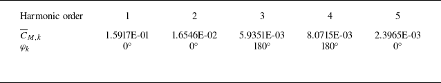
are the amplitude and phase of the kth harmonic, respectively. The coefficients of the first five harmonics amplitudes and phases are listed in table 2. The amplitude of the second harmonic
$\varphi _{k}$
are the amplitude and phase of the kth harmonic, respectively. The coefficients of the first five harmonics amplitudes and phases are listed in table 2. The amplitude of the second harmonic $\overline{C}_{M,2}$
is only 10.4 % of
$\overline{C}_{M,2}$
is only 10.4 % of $\overline{C}_{M,1}$
, indicating the dominance of the first harmonic. The fitted curves of
$\overline{C}_{M,1}$
, indicating the dominance of the first harmonic. The fitted curves of $\overline{C}_{\textit{MS}}$
using (4.1) considering the first five harmonics are shown in figure 9, and they agree well with the calculated results.
$\overline{C}_{\textit{MS}}$
using (4.1) considering the first five harmonics are shown in figure 9, and they agree well with the calculated results.
4.2.1. Biased vibration at V r = 4 in case A
In case A, V
r
= 4 is a special case where the angular displacement remains negative (figure 5
a). Figure 9 indicates that in case A, a very small $\theta ^{*}$
value (<0.5) is in an excitation range where the directions of the fluid moment and the angular displacement are the same. At very small reduced velocities V
r
= 1–3, because the spring is relatively very rigid, the spring moment can make the TP rotate back and forth crossing the
$\theta ^{*}$
value (<0.5) is in an excitation range where the directions of the fluid moment and the angular displacement are the same. At very small reduced velocities V
r
= 1–3, because the spring is relatively very rigid, the spring moment can make the TP rotate back and forth crossing the $\theta ^{*}=0$
line, making the vibration symmetric. The rotation angle
$\theta ^{*}=0$
line, making the vibration symmetric. The rotation angle $\theta ^{*}$
of V
r
= 4 is always negative because it is trapped in the excitation range. To make the vibration escape from the excitation range,
$\theta ^{*}$
of V
r
= 4 is always negative because it is trapped in the excitation range. To make the vibration escape from the excitation range, $\theta ^{*}$
must cross the boundary of the excitation range, which is
$\theta ^{*}$
must cross the boundary of the excitation range, which is $\theta ^{*}=0.5$
. This needs a torque coefficient that is greater than its maximum value within
$\theta ^{*}=0.5$
. This needs a torque coefficient that is greater than its maximum value within $| \theta ^{*}| \lt 0.5$
, which is
$| \theta ^{*}| \lt 0.5$
, which is $C_{M,\textit{max}}=\max (\overline{C}_{\textit{MS}}+A_{\textit{CMS}})=0.252$
measured from figure 9. Considering the balance between the spring moment and the fluid moment for a stationary TP, i.e.
$C_{M,\textit{max}}=\max (\overline{C}_{\textit{MS}}+A_{\textit{CMS}})=0.252$
measured from figure 9. Considering the balance between the spring moment and the fluid moment for a stationary TP, i.e. ${4\pi ^{2}\theta}/{{V}_{r}^{2}} ={C_{M,\textit{max}}}/({2J_{r}})$
(removing the motion terms
${4\pi ^{2}\theta}/{{V}_{r}^{2}} ={C_{M,\textit{max}}}/({2J_{r}})$
(removing the motion terms $\dot{\theta }$
and
$\dot{\theta }$
and $\ddot{\theta }$
, and replacing
$\ddot{\theta }$
, and replacing $C_{\!{M}}$
with
$C_{\!{M}}$
with $C_{M,\textit{max}}$
, in (2.3)) the critical reduced velocity for the TP to escape the non-zero mean
$C_{M,\textit{max}}$
, in (2.3)) the critical reduced velocity for the TP to escape the non-zero mean $\theta ^{*}$
is
$\theta ^{*}$
is $V_{r,cr}=4.86$
. In the numerical simulation, the response was trapped in the excitation zone at
$V_{r,cr}=4.86$
. In the numerical simulation, the response was trapped in the excitation zone at $V_{r}=4$
, and escaped it at
$V_{r}=4$
, and escaped it at $V_{r}=5$
.
$V_{r}=5$
.
Harmonic components of $\overline{C}_{\textit{MS}}$
for (4.1).
$\overline{C}_{\textit{MS}}$
for (4.1).

The time histories of the rotational angle, rotational speed, fluid moment and non-dimensional spring moment are shown in figure 10(a) to further illustrate why the angular displacement remains negative at V
r
= 4 in case A. Following (2.3), the non-dimensional fluid moment ( $M^{*}$
) and spring moment (
$M^{*}$
) and spring moment ( ${M}_{s}^{*}$
) are defined as
${M}_{s}^{*}$
) are defined as $M^{*}=C_{M}/(2J_{r})$
,
$M^{*}=C_{M}/(2J_{r})$
, ${M}_{s}^{*}=-4\pi ^{2}\theta /{V}_{r\theta }^{2}$
, respectively, in the figure. The non-dimensional fluid moment remains negative all the time, resulting in a negative mean angular deflection of the TP.
${M}_{s}^{*}=-4\pi ^{2}\theta /{V}_{r\theta }^{2}$
, respectively, in the figure. The non-dimensional fluid moment remains negative all the time, resulting in a negative mean angular deflection of the TP.
Variation of the angular displacement $\theta ^{*}$
, angular velocity
$\theta ^{*}$
, angular velocity $\dot{\theta }^{*}$
, fluid moment
$\dot{\theta }^{*}$
, fluid moment $M^{*}$
and spring moment
$M^{*}$
and spring moment ${M}_{s}^{*} -{4\pi ^{2}\theta}/{{\omega }_{r}^{2}}$
for (a) for
${M}_{s}^{*} -{4\pi ^{2}\theta}/{{\omega }_{r}^{2}}$
for (a) for $V_r=4$
and (b)
$V_r=4$
and (b) $V_r =24$
in case A.
$V_r =24$
in case A.

The non-zero, one-sided mean deflection found at V
r
= 4 in case A is not found in case B because the excitation zone $| \theta ^{*}| \leq 0.5$
of case A becomes damping zones in case B, as shown in figure 9. Because
$| \theta ^{*}| \leq 0.5$
of case A becomes damping zones in case B, as shown in figure 9. Because $| \theta ^{*}| \leq 0.5$
is the damping range in case B, deflection angle
$| \theta ^{*}| \leq 0.5$
is the damping range in case B, deflection angle $| \theta ^{*}| \leq 0.5$
in one direction results in a fluid moment in the direction opposite to θ, and this moment acts as a recover moment to pull the TP back and cross θ = 0.
$| \theta ^{*}| \leq 0.5$
in one direction results in a fluid moment in the direction opposite to θ, and this moment acts as a recover moment to pull the TP back and cross θ = 0.
4.2.2. Values of
${\theta }_{m}^{\mathrm{*}}$
falling into damping ranges at smaller reduced velocities

Why the maximum vibration angle mainly falls into damping ranges at smaller reduced velocities but not excitation ranges can be explained by observing the force of a stationary TP like in the case of transverse galloping (Barrero-Gil, Sanz-Andrés & Roura Reference Barrero-Gil, Sanz-Andrés and Roura2009; Joly, Etienne & Pelletier Reference Joly, Etienne and Pelletier2012). During vibration the instantaneous $C_{M}$
follows the same trend as
$C_{M}$
follows the same trend as $\overline{C}_{\textit{MS}}$
when the rotation angle reaches its maximum/minimum values, as shown in figure 11. In the figure,
$\overline{C}_{\textit{MS}}$
when the rotation angle reaches its maximum/minimum values, as shown in figure 11. In the figure, $\overline{C}_{\textit{MS}}$
is calculated using the instantaneous
$\overline{C}_{\textit{MS}}$
is calculated using the instantaneous $\theta ^{*}$
based on (4.1). When TP is rotating to its maximum position in a damping range, where the rotation velocity approaches zero,
$\theta ^{*}$
based on (4.1). When TP is rotating to its maximum position in a damping range, where the rotation velocity approaches zero, $\overline{C}_{\textit{MS}}$
is in the opposite direction to the rotation angle. In figure 11(b), CM
is not the same as
$\overline{C}_{\textit{MS}}$
is in the opposite direction to the rotation angle. In figure 11(b), CM
is not the same as $\overline{C}_{\textit{MS}}$
when
$\overline{C}_{\textit{MS}}$
when $\theta ^{*}$
is approaching
$\theta ^{*}$
is approaching ${\theta }_{m}^{*}$
, but it follows the same trend as
${\theta }_{m}^{*}$
, but it follows the same trend as $\overline{C}_{\textit{MS}}$
, i.e. its value reduces significantly to nearly zero in figure 11(b). The significant reduction of CM
makes the rotation reverse its direction, leaving a maximum rotation angle in this damping range. The rotation cannot change its direction in an excitation range because the moment
$\overline{C}_{\textit{MS}}$
, i.e. its value reduces significantly to nearly zero in figure 11(b). The significant reduction of CM
makes the rotation reverse its direction, leaving a maximum rotation angle in this damping range. The rotation cannot change its direction in an excitation range because the moment $\overline{C}_{\textit{MS}}$
accelerates the rotation in excitation ranges.
$\overline{C}_{\textit{MS}}$
accelerates the rotation in excitation ranges.
Time histories of $\theta ^{*}$
,
$\theta ^{*}$
, $C_{M}$
and
$C_{M}$
and $\overline{C}_{\textit{MS}}$
to visualise the correlation between
$\overline{C}_{\textit{MS}}$
to visualise the correlation between $C_{M}$
and
$C_{M}$
and $\overline{C}_{\textit{MS}}$
.
$\overline{C}_{\textit{MS}}$
.

Values of $C_{M}$
and
$C_{M}$
and $\overline{C}_{\textit{MS}}$
are more correlated to each other at larger reduced velocities in case A (>22). In figure 11(c), where V
r
= 40,
$\overline{C}_{\textit{MS}}$
are more correlated to each other at larger reduced velocities in case A (>22). In figure 11(c), where V
r
= 40, $C_{M}$
and
$C_{M}$
and $\overline{C}_{\textit{MS}}$
oscillate with nearly the same frequency, but because of the rotation, the magnitude of
$\overline{C}_{\textit{MS}}$
oscillate with nearly the same frequency, but because of the rotation, the magnitude of $C_{M}$
is smaller. Whenever the rotation angle
$C_{M}$
is smaller. Whenever the rotation angle $\theta ^{*}$
is in a damping range
$\theta ^{*}$
is in a damping range $n+0.5\leq \theta ^{*}\leq n+1$
, both
$n+0.5\leq \theta ^{*}\leq n+1$
, both $C_{M}$
and
$C_{M}$
and $\overline{C}_{\textit{MS}}$
are in the direction opposite to
$\overline{C}_{\textit{MS}}$
are in the direction opposite to $\theta ^{*}$
. In figure 11(b), the correlation between
$\theta ^{*}$
. In figure 11(b), the correlation between $C_{M}$
and
$C_{M}$
and $\overline{C}_{\textit{MS}}$
becomes weak, but their maximum and minimum values occur simultaneously most of the time. The correlation coefficient
$\overline{C}_{\textit{MS}}$
becomes weak, but their maximum and minimum values occur simultaneously most of the time. The correlation coefficient $R_{M}$
between
$R_{M}$
between $C_{M}$
and
$C_{M}$
and $\overline{C}_{\textit{MS}}$
is calculated as
$\overline{C}_{\textit{MS}}$
is calculated as
 \begin{equation}R_{M}=\frac{\sum \left[\left(C_{M}-\overline{C}_{M}\right)\left(\overline{C}_{\textit{MS}}-\overline{\overline{C}_{\textit{MS}}}\right)\right]}{\sqrt{\sum \left(C_{M}-\overline{C}_{M}\right)^{2}}\sqrt{\sum \left(\overline{C}_{\textit{MS}}-\overline{\overline{C}_{\textit{MS}}}\right)^{2}}}.\end{equation}
Figure 12 shows the correlation coefficients $R_{M}$
of cases A, B and C. The correlation coefficients at very small velocities (V
r
= 1–3), where both vibration and vortex shedding are dominated by the Strouhal number, are either 1 or –1 because when the prism vibrates at very small amplitude,
$R_{M}$
of cases A, B and C. The correlation coefficients at very small velocities (V
r
= 1–3), where both vibration and vortex shedding are dominated by the Strouhal number, are either 1 or –1 because when the prism vibrates at very small amplitude, $C_{M}$
and
$C_{M}$
and $\overline{C}_{\textit{MS}}$
oscillate with the same frequency, but they are out of phase with each other in cases B and C. When the reduced velocity exceeds 22, the correlation coefficient
$\overline{C}_{\textit{MS}}$
oscillate with the same frequency, but they are out of phase with each other in cases B and C. When the reduced velocity exceeds 22, the correlation coefficient $R_{M}$
is above 0.5 and does not very much with V
r
in all cases. The correlation is good, although not ideally 1, indicating that using
$R_{M}$
is above 0.5 and does not very much with V
r
in all cases. The correlation is good, although not ideally 1, indicating that using $\overline{C}_{\textit{MS}}$
to explain galloping is appropriate. When galloping of an object in the crossflow direction was investigated, the division of the excitation ranges and damping ranges does not exist because the arrangement of the objects related to the flow remain the same. For the rotational vibration with a large amplitude, the TP goes through multiple excitation and damping ranges, and finally reaches maximum angle and reverses at the upper boundary of a damping range. The vibration does not reverse at the upper boundary of an excitation range or within an excitation range because once the TP enters an excitation range,
$\overline{C}_{\textit{MS}}$
to explain galloping is appropriate. When galloping of an object in the crossflow direction was investigated, the division of the excitation ranges and damping ranges does not exist because the arrangement of the objects related to the flow remain the same. For the rotational vibration with a large amplitude, the TP goes through multiple excitation and damping ranges, and finally reaches maximum angle and reverses at the upper boundary of a damping range. The vibration does not reverse at the upper boundary of an excitation range or within an excitation range because once the TP enters an excitation range, $C_{M}$
– which is in the same direction as the rotational angle and speed – further accelerates the vibration speed and lets
$C_{M}$
– which is in the same direction as the rotational angle and speed – further accelerates the vibration speed and lets $\theta ^{*}$
pass this excitation range.
$\theta ^{*}$
pass this excitation range.
Correlation coefficient between $C_{M}$
and
$C_{M}$
and $\overline{C}_{\textit{MS}}$
.
$\overline{C}_{\textit{MS}}$
.

4.2.3. Values of
${\theta }_{m}^{\mathrm{*}}$
are close to the upper boundaries of the damping ranges at larger reduced velocities

At large reduced velocities ( $V_{r\theta }\geq 12$
,
$V_{r\theta }\geq 12$
, $V_{r\theta }\geq 22$
and
$V_{r\theta }\geq 22$
and $V_{r\theta }\geq 16$
, in cases A, B and C, respectively), the maximum values
$V_{r\theta }\geq 16$
, in cases A, B and C, respectively), the maximum values ${\theta }_{m}^{*}$
are mostly close to
${\theta }_{m}^{*}$
are mostly close to $\gamma ^{*}=\theta ^{*}+{\gamma }_{0}^{*}=n$
, which are the upper boundaries of the damping zones. In case A,
$\gamma ^{*}=\theta ^{*}+{\gamma }_{0}^{*}=n$
, which are the upper boundaries of the damping zones. In case A, ${\theta }_{m}^{*}$
values are mainly close to
${\theta }_{m}^{*}$
values are mainly close to $| \theta ^{*}| =2$
, 3 and 4, and no amplitudes are found close to
$| \theta ^{*}| =2$
, 3 and 4, and no amplitudes are found close to $| \theta ^{*}| =2.5$
, 3.5 or 4.5, as seen in figure 7. The reason why
$| \theta ^{*}| =2.5$
, 3.5 or 4.5, as seen in figure 7. The reason why ${\theta }_{m}^{*}$
is not close to the upper boundary of an excitation range is that after being accelerated in an excitation range, the TP always gains sufficient momentum to rotate across the upper boundary of this excitation range due to inertia. How the angular displacement reaches its maximum and minimum values and reverses at an exemplar case V
r
= 24 can be further explained by observing the time histories of the vibration displacement, velocity and moment in figure 10(b). When the displacement is approaching its maximum and minimum values at times marked by vertical dash-dotted lines in the figure, the fluid moment is opposite to the directions of both velocity and displacement, and the spring moment is at its maximum. While the kinetic energy of the TP is nearly zero, the fluid moment and the spring moment that are in the opposition direction of the velocity make the rotation reverse. The fluid moment oscillates with a frequency much higher than the principal frequency of the angular displacement because flow goes through multiple periods of vortex shedding within one period of vibration. The fluid velocity also has high frequency component under the influence of the high-frequency oscillation of the fluid moment.
${\theta }_{m}^{*}$
is not close to the upper boundary of an excitation range is that after being accelerated in an excitation range, the TP always gains sufficient momentum to rotate across the upper boundary of this excitation range due to inertia. How the angular displacement reaches its maximum and minimum values and reverses at an exemplar case V
r
= 24 can be further explained by observing the time histories of the vibration displacement, velocity and moment in figure 10(b). When the displacement is approaching its maximum and minimum values at times marked by vertical dash-dotted lines in the figure, the fluid moment is opposite to the directions of both velocity and displacement, and the spring moment is at its maximum. While the kinetic energy of the TP is nearly zero, the fluid moment and the spring moment that are in the opposition direction of the velocity make the rotation reverse. The fluid moment oscillates with a frequency much higher than the principal frequency of the angular displacement because flow goes through multiple periods of vortex shedding within one period of vibration. The fluid velocity also has high frequency component under the influence of the high-frequency oscillation of the fluid moment.
4.3. Vortex shedding
Figure 13 shows contours of vorticity at V
r
= 17 in case A to visualise the wake. The maximum angle in the negative θ-direction is approximately half that in the positive θ-direction. The vortex shedding is asymmetric because the maximum and minimum values of the angular displacement are different from each other. The numbers of vortices that are shed from one half-period is correlated to the angular vibration amplitude. During the time from t = 429 to t = 437, the vibration angle is negative, with minimum value ${\theta }_{\textit{min}}^{*}=-0.91$
, and a pair of vortices (vortices 1 and 2) is shed from the cylinder. During the time from t = 437 to t = 451, the vibration angle is positive, with maximum value
${\theta }_{\textit{min}}^{*}=-0.91$
, and a pair of vortices (vortices 1 and 2) is shed from the cylinder. During the time from t = 437 to t = 451, the vibration angle is positive, with maximum value ${\theta }_{\textit{max}}^{*}=1.72$
, and two and a half pairs of vortices are shed from the cylinder (vortices 3, 4, 5a, 5b and 6). Because vortices 5a and 5b are generated from a same free shear layer, there are two periods of vortex shedding between instants (b) and (c).
${\theta }_{\textit{max}}^{*}=1.72$
, and two and a half pairs of vortices are shed from the cylinder (vortices 3, 4, 5a, 5b and 6). Because vortices 5a and 5b are generated from a same free shear layer, there are two periods of vortex shedding between instants (b) and (c).
Contours of vorticity for V r = 17 in case A.

Figure 14 shows the flow near the TP for the same case as in figure 13 visualised by contours of the pressure coefficient and streamlines. The pressure coefficient is defined as $C_{p}={2(p-p_{0})}/({\rho DU^{2}})$
, where
$C_{p}={2(p-p_{0})}/({\rho DU^{2}})$
, where $p_{0}$
is the pressure of the undisturbed flow. The stagnation point indicated by a small circle in the figure is the point where the maximum pressure occurs. The three vertices of the TP are labelled by 1–3, respectively, to assist in the visualisation of the rotation. For a bluff body with sharp corners, the separation points are located at the vertices of the body (Zhou, Hao & Alam Reference Zhou, Hao and Alam2024), and this was what was observed in figure 14. Based on the streamlines, one can see that the separation points of the flow are always located at vertices of the cylinder, except for the most upstream vertex that directly faces the flow at t = 429.3, 437.1 and 444.6. When a side boundary is slightly inclined relative to the flow (e.g. boundary 2–3 at t = 435.4), the separated flow from the upstream vertex 2 reattaches to the downstream vertex 3 and separates again; as a result, flow separation occurs at three vertices. The stagnation point is always located at the upstream side boundary. It moves in the opposite direction to the rotation along the surface of the TP. The stagnation point reaches the most upstream vertex when
$p_{0}$
is the pressure of the undisturbed flow. The stagnation point indicated by a small circle in the figure is the point where the maximum pressure occurs. The three vertices of the TP are labelled by 1–3, respectively, to assist in the visualisation of the rotation. For a bluff body with sharp corners, the separation points are located at the vertices of the body (Zhou, Hao & Alam Reference Zhou, Hao and Alam2024), and this was what was observed in figure 14. Based on the streamlines, one can see that the separation points of the flow are always located at vertices of the cylinder, except for the most upstream vertex that directly faces the flow at t = 429.3, 437.1 and 444.6. When a side boundary is slightly inclined relative to the flow (e.g. boundary 2–3 at t = 435.4), the separated flow from the upstream vertex 2 reattaches to the downstream vertex 3 and separates again; as a result, flow separation occurs at three vertices. The stagnation point is always located at the upstream side boundary. It moves in the opposite direction to the rotation along the surface of the TP. The stagnation point reaches the most upstream vertex when $\theta ^{*}$
is very close to an integer number n (t = 429.3 and 433.6). At t = 444.6, the vibration angle reaches its maximum value
$\theta ^{*}$
is very close to an integer number n (t = 429.3 and 433.6). At t = 444.6, the vibration angle reaches its maximum value ${\theta }_{m}^{*}= 1.72$
, whichis much smaller than 2; as a result, the stagnation point did not reach vertex 3.
${\theta }_{m}^{*}= 1.72$
, whichis much smaller than 2; as a result, the stagnation point did not reach vertex 3.
Contours of the pressure coefficient and streamlines during one and a half periods of vibration for Vr = 17 in case A.

(a–s) Contours of vorticity in two periods of vibration. The bottom graph shows time histories of the angular displacement and moment coefficient for case A and V
r
= 40. The displacement $\theta ^{*}$
at every instant, and the number of vortex pairs that are shed from the TP between two instants, are labelled.
$\theta ^{*}$
at every instant, and the number of vortex pairs that are shed from the TP between two instants, are labelled.

Figures 15(a–s) show the contours of the vorticity for V
r
= 40 in case A at all the instants where the angular displacements are close to integer numbers. These instants are labelled on the time histories of the angular displacement and moment coefficient at the bottom of figure 15. Because the vibration is very aperiodic, the wake pattern at the beginning of a vibration period is very different from that at the end of this period. The maximum angular displacement is ${\theta }_{max }^{*}=5$
in the period between instants (a) and (k), and
${\theta }_{max }^{*}=5$
in the period between instants (a) and (k), and ${\theta }_{\textit{min}}^{*}=-4$
between instants (k) and (s). In most of the time intervals where
${\theta }_{\textit{min}}^{*}=-4$
between instants (k) and (s). In most of the time intervals where $\theta ^{*}$
either increases or decreases by 1, the moment coefficient oscillates for one period, and the number of vortices that are shed from the TP is one pair, but with exceptions. Examples of exceptions include no vortex shedding between (b) and (c), and two pairs of vortices shed from the TP between (n) and (o). If one pair of vortices is shed from the TP when
$\theta ^{*}$
either increases or decreases by 1, the moment coefficient oscillates for one period, and the number of vortices that are shed from the TP is one pair, but with exceptions. Examples of exceptions include no vortex shedding between (b) and (c), and two pairs of vortices shed from the TP between (n) and (o). If one pair of vortices is shed from the TP when $\theta ^{*}$
either increases or decreases by 1, then the number of the vortex pair within a half-period of the vibration amplitude should be
$\theta ^{*}$
either increases or decreases by 1, then the number of the vortex pair within a half-period of the vibration amplitude should be $2\,| {\theta }_{m}^{*}|$
; here, a half-period is defined as the duration when
$2\,| {\theta }_{m}^{*}|$
; here, a half-period is defined as the duration when $\theta ^{*}$
of the TP remains either positive or negative, i.e. (a)–(k) and (k)–(s) in figure 15. The number of vortices in the half-period between (a) and (k), where
$\theta ^{*}$
of the TP remains either positive or negative, i.e. (a)–(k) and (k)–(s) in figure 15. The number of vortices in the half-period between (a) and (k), where ${\theta }_{max }^{*}=5$
, is 8 instead of 10, because there is no vortex during (b)–(c) and (h)–(i). The number of vortices in the half-period between (k) and (s), where
${\theta }_{max }^{*}=5$
, is 8 instead of 10, because there is no vortex during (b)–(c) and (h)–(i). The number of vortices in the half-period between (k) and (s), where ${\theta }_{\textit{min}}^{*}=-4$
, is 5 pairs.
${\theta }_{\textit{min}}^{*}=-4$
, is 5 pairs.
Because the vortex shedding processes of most of the simulated reduced velocities are very aperiodic and not repeatable, no attempt was made to classify the vortex shedding of all simulated reduced velocities into different categories. The moment coefficient oscillates for one period when $\theta ^{*}$
either increases or decreases by 1 in most of the cases, even when there is no vortex shedding, because the motion of vortices, e.g. the split of vortex 3 in figure 15(c), causes oscillation of the moment coefficient.
$\theta ^{*}$
either increases or decreases by 1 in most of the cases, even when there is no vortex shedding, because the motion of vortices, e.g. the split of vortex 3 in figure 15(c), causes oscillation of the moment coefficient.
5. Conclusions
Flow-induced torsional galloping of a triangular prism (TP) is investigated numerically at m
* = 2 and Re = 150. Because the prism is geometrically periodic along the rotational direction, with period 2π/3, the normalised rotation angle is defined as $\theta ^{*}=\theta /(2\pi /3)$
for the convenience of discussion. The conclusions are summarised below.
$\theta ^{*}=\theta /(2\pi /3)$
for the convenience of discussion. The conclusions are summarised below.
Three configurations are considered (see figure 1): case A where one vertex of the TP section faces the flow, case B where one boundary of the TP section faces the flow, and case C, which is an asymmetric case. In all cases, the response is galloping where the angular amplitude of the vibration increases continuously with the increase of reduced velocity. The TP gallops at a frequency much lower than the dominant frequency of the fluid moment and vortex shedding frequency.
The response of the TP is correlated to the fluid moment of a stationary TP. The mean moment ( $\overline{C}_{\textit{MS}}$
) of a stationary TP with various rotation angles is calculated, and the rotation angles are divided into damping ranges where the fluid moment and the rotational angle are in opposite directions, and excitation ranges where the fluid moment and the rotational angle are in the same direction. In all three cases, the excitation ranges are
$\overline{C}_{\textit{MS}}$
) of a stationary TP with various rotation angles is calculated, and the rotation angles are divided into damping ranges where the fluid moment and the rotational angle are in opposite directions, and excitation ranges where the fluid moment and the rotational angle are in the same direction. In all three cases, the excitation ranges are $n\leq \gamma ^{*}=\theta ^{*}+{\gamma }_{0}^{*}\leq n+0.5$
, and the damping ranges are
$n\leq \gamma ^{*}=\theta ^{*}+{\gamma }_{0}^{*}\leq n+0.5$
, and the damping ranges are $n\leq \gamma ^{*}=\theta ^{*}+{\gamma }_{0}^{*}\leq n+0.5$
. The excitation ranges of case A are the damping ranges of case B, and vice versa. When the reduced velocity is smaller than a critical value, the vibration amplitude is dominated by a single amplitude in the damping ranges (see figure 7), and this critical value is
$n\leq \gamma ^{*}=\theta ^{*}+{\gamma }_{0}^{*}\leq n+0.5$
. The excitation ranges of case A are the damping ranges of case B, and vice versa. When the reduced velocity is smaller than a critical value, the vibration amplitude is dominated by a single amplitude in the damping ranges (see figure 7), and this critical value is $12$
,
$12$
, $22$
and
$22$
and $16$
for cases A, B and C, respectively. The maximum rotation angle does not occur within an excitation range because the same direction between the fluid moment and the rotational angle always makes the TP rotate outside these ranges.
$16$
for cases A, B and C, respectively. The maximum rotation angle does not occur within an excitation range because the same direction between the fluid moment and the rotational angle always makes the TP rotate outside these ranges.
When the reduced velocity is greater than the critical value, the amplitude of each reduced velocity varies very much with time, and the vibration is dominated by multiple amplitudes, each of them close to the upper boundary of a damping range. At large reduced velocities, the maximum rotation angle changes from period to period, but the maximum rotation angles relative to the reference position ${\gamma }_{m}^{*}={\theta }_{0}^{*}+{\gamma }_{0}^{*}$
are close to integer numbers (n) in all cases, which are upper boundaries of damping ranges.
${\gamma }_{m}^{*}={\theta }_{0}^{*}+{\gamma }_{0}^{*}$
are close to integer numbers (n) in all cases, which are upper boundaries of damping ranges.
In case A,V
r
= 4 is a transition reduced velocity where the vibration transitions from vortex shedding dominant vibration to galloping. The vibration of the TP at V
r
= 4 is deflected to one direction, resulting in a non-zero mean displacement. The vibration deflects to one direction because $| \theta ^{*}| \leq 0.5$
is an excitation range where the moment
$| \theta ^{*}| \leq 0.5$
is an excitation range where the moment $\overline{C}_{\textit{MS}}$
and
$\overline{C}_{\textit{MS}}$
and $\theta ^{*}$
are in the same direction.
$\theta ^{*}$
are in the same direction.
Because the galloping is very aperiodic and no repeating patterns are found in the vortex shedding, no attempt was made to classify the vortex shedding into distinct modes. It was found that whenever the non-dimension angular displacement increases or decreases by 1, one pair of vortices is shed from the galloping TP in most cases, but with some exceptions where either zero pairs or two pairs of vortices are shed.
Declaration of interests
The author reports no conflict of interest.


 Open access