


1. Introduction
Squeak and rattle (S&R) refer to unexpected, irregular and annoying noises inside the car cabin. The continuous improvements in attenuating the stationary types of sounds in passenger cars (Harrison Reference Harrison2004), the introduction of electric engines and the new prospects for alternative uses of cars as a result of autonomous driving has caused the S&R complaints to remain among the top warranty issues in passenger cars (Trapp & Chen Reference Trapp and Chen2012; Sprenger Reference Sprenger2017). S&R events happen when the neighbouring interfaces come into contact. Rattle sound is an impact sound resulting from the frequent impulsive impact events in an assembly interface (Kavarana & Rediers Reference Kavarana and Rediers1999; Trapp & Chen Reference Trapp and Chen2012). Squeak is a friction-induced sound caused by the dynamic instabilities during friction events such as the stick-slip, the sprag-slip and the mode-coupling instabilities (Elmaian et al. Reference Elmaian, Gautier, Pezerat and Duffal2014). In stick-slip events, as one of the main mechanisms behind the squeak generation, the frequent and subsequent interchange of strain and kinetic energy in the planar motion event in the contact interface generates a high-frequency annoying noise known as squeak. One of the main provisions to avoid S&R in passenger cars is to control the interface clearances and preloads in subsystem assemblies. Thus, the static and dynamic relative motion of neighbouring parts in critical interfaces for S&R are needed to be controlled (Daams Reference Daams2009; Trapp & Chen Reference Trapp and Chen2012). This can be achieved by robust design techniques and controlling the dynamic response of the system. During the predesign-freeze phases of the passenger car development, robust design analyses involve stability analysis (Söderberg & Lindkvist Reference Söderberg and Lindkvist1999) and contribution analysis (Söderberg et al. Reference Söderberg, Lindkvist, Wärmefjord and Carlson2016) that are referred to as geometry assurance. The dynamic response can be controlled by avoiding resonance and blocking the force transfer paths in a product assembly. To address these problems efficiently, robustly and affordably, measures need to be taken that concern the design concepts of the product. For this purpose, automakers adopt actions such as connection configuration management in assemblies, material selection, structural properties definition and part geometrical modifications (Trapp & Chen Reference Trapp and Chen2012; Bayani Reference Bayani2020). Today, optimisation tools for maximising the product quality by controlling the cost are practically available for different attributes during the product design phase. Design activities related to the S&R attribute cannot be excepted from the optimisation loops in attribute balancing processes. However, the involvement of nonrigid robust design analysis in closed-loop optimisation processes in the design phase to reduce the risk for S&R remains limited. An optimisation approach was proposed by Bayani et al. (Reference Bayani, Wickman, Lindkvist and Söderberg2022 b) to determine the connection configuration in an assembly to minimise the risk for S&R by improving the geometric robustness. However, the robustness of the clearances and preloads in the critical interfaces for S&R are required to be ensured by other measures as well, such as introducing structural reinforcements and geometrical features for assembly components. These geometrical modifications can be determined by optimisation processes, such as topometry optimisation and topology optimisation. Today, the evaluation of the robustness of the resultant design is done decoupled from the geometry optimisation process. In this respect, computational cost and the lack of tools to embed robustness objectives for S&R have been the main obstructions. Since design robustness is crucial for S&R, in this article a method is proposed to involve geometric variation analysis in the structural optimisation process with the aim of minimising the risk for S&R. The proposed optimisation method involves a stage-wise procedure to address the computational inefficiency of the available gradient-based methods. In an industrial case, the proposed method was used in a multidisciplinary topometry optimisation to determine geometrical patterns in a component of an assembly that required reinforcement. The optimisation objectives involved the estimated risk for S&R generation from design robustness and dynamic response perspectives.
2. Aim and contribution of the work
Since geometric variation is a key contributor to S&R problems (Gosavi Reference Gosavi2005; Daams Reference Daams2009; Trapp & Chen Reference Trapp and Chen2012), design robustness analyses should be involved in the design process of the automotive parts and assemblies to avoid S&R events by implementing concept-related solutions. Despite this, in practice, geometric variation analysis is done decoupled from the component structural optimisation in the design phase. There is a lack of optimisation tools and methods specifically developed to address this problem. Besides, the simulation time of utilising the available topometry optimisation tools and methods is unaffordable in the industry when geometric simulations are required to calculate the optimisation objectives. Thus, the main aim of this work is to propose a method to involve the geometric variation analysis in the topometry optimisation process in an affordable way to minimise the risk for S&R. By monitoring the system response in terms of the risk for S&R generation, it is shown that topometry optimisation can be done in a stepwise approach by involving robust design and dynamic response analyses. The proposed method can lead to reducing the risk for S&R by actively involving geometric variation analysis in the closed-loop structural design processes. This may enhance the involvement of the S&R attribute in attribute balancing activities during the predesign-freeze phases of car development.
3. Quantified S&R evaluation
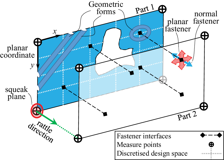
Consider the schematic subsystem assembly of two parts shown in Figure 1. The two parts are assembled by realised fasteners that can be located by using an optimisation process as proposed by Bayani et al. (Reference Bayani, Wickman, Lindkvist and Söderberg2022 b). To further reduce the risk for S&R, the components in an assembly might need local and global structural reinforcements as the geometric forms in part 1 in Figure 1. To determine these geometric forms in an optimisation process, the risk for the generation of S&R is required to be determined in a quantified way. In this work, the optimisation objectives were considered as the S&R risk severity metrics previously proposed in Bayani et al. Reference Bayani, Wickman, Krishnaswamy, Sathappan and Söderberg2022 a,b. For this purpose, the system response needs to be evaluated in the measure points located at the preidentified interfaces for S&R. These interfaces can be determined through a systematic way called contact point analysis as described by Daams (Reference Daams2009). Similar to Bayani et al. (Reference Bayani, Wickman, Krishnaswamy, Sathappan and Söderberg2022 a,b), the rattle risk severity factors were calculated in the rattle direction, which is the normal direction between the two surfaces in a critical interface. At every interface, the squeak risk severity factor was calculated in the squeak plane that is the normal plane to the rattle direction. Then, the total risk may be considered as a weighted sum of the calculated risk factors in the rattle direction and the squeak plane. In this work, the calculated S&R risk severity metrics were given equal importance.
The schematic depiction of an assembly of two parts involving the connection configuration, the S&R measure points and the geometrical forms at the component level.
3.1. Geometric robustness and S&R
Controlling the static and dynamic clearance and preloads in the critical interfaces for S&R is the main concept-related solution to minimise the risk for the generation of S&R (Trapp & Chen Reference Trapp and Chen2012). The significance of considering the geometric variation results for reducing the risk for S&R generation has been discussed in the literature (Gosavi Reference Gosavi2005; Daams Reference Daams2009; Trapp & Chen Reference Trapp and Chen2012). Design factors that contribute to geometric variation management, such as the part-or assembly-level manufacturing variations, connection configuration in an assembly (Söderberg et al. Reference Söderberg, Wärmefjord, Lindkvist and Berlin2012), material properties, form and structural properties of parts can change the clearance and interface forces (Wärmefjord, Söderberg & Lindkvist Reference Wärmefjord, Söderberg and Lindkvist2013) in critical interfaces for S&R. This can potentially increase the risk for S&R generation by causing the poor control of the relative motion of the parts in the S&R critical interfaces (Kavarana & Rediers Reference Kavarana and Rediers1999; Trapp & Chen Reference Trapp and Chen2012). Indeed, deviation from the nominal gap and the prescribed assembly preloads might increase the risk for the impact and the unstable friction events that are the principal phenomena behind the generation of S&R. Despite the importance of geometric variation in preventing S&R, the practical use of geometric variation analysis limits to adjusting the interface clearance targets in design evaluation analyses, such as the clearance considerations in S&R contact point analysis (Daams Reference Daams2009) and structural dynamic simulations to analyse S&R events (Naganarayana et al. Reference Naganarayana, Shankar, Bhattachar, Brines and Rao2003; Trapp & Chen Reference Trapp and Chen2012; Weber & Benhayoun Reference Weber and Benhayoun2012; Benhayoun et al. Reference Benhayoun, Bonin, Millet de Faverges and Massaon2017).
Geometry assurance (Söderberg et al. Reference Söderberg, Lindkvist, Wärmefjord and Carlson2016) refers to a set of activities aiming at minimising the effect of manufacturing geometrical variations on the quality of the final product. These activities involve robust design analysis such as stability analysis (Söderberg & Lindkvist Reference Söderberg and Lindkvist1999) and contribution analysis (Söderberg et al. Reference Söderberg, Lindkvist, Wärmefjord and Carlson2016) with the aid of Computer Aided Tolerancing (CAT) tools. Different methods and models for geometric variation simulation are reviewed in Shen et al. (Reference Shen, Ameta, Shah and Davidson2005), Cao, Liu & Yang (Reference Cao, Liu and Yang2018) and Morse et al. (Reference Morse, Dantan, Anwer, Söderberg, Moroni, Qureshi, Jiang and Mathieu2018). Interior trim parts causing the in-cabin S&R problems are often made of plastic material or include large flexible panels. For these flexible bodies, using nonrigid geometric variation models increase the accuracy of the analysis, such as the variation model (Gupta & Turner Reference Gupta and Turner1993), deviation domain model (Giordano, Samper & Petit Reference Giordano, Samper and Petit2007) and skin model shapes (Mathieu & Ballu Reference Mathieu and Ballu2007; Schleich et al. Reference Schleich, Anwer, Mathieu and Wartzack2014). For this purpose, the implementation of finite element (FE) techniques in geometric variation analysis has been proposed (Cai, Hu & Yuan Reference Cai, Hu and Yuan1996; Charles Liu & Jack Hu Reference Charles Liu and Jack Hu1997). However, the computational cost is a definitive factor in using nonrigid geometric variation simulation. To address this drawback, different methods have been introduced, such as the number theoretical net (NT-net) (Huang Reference Huang2013), the method proposed by Corrado & Polini (Reference Corrado and Polini2018) to use skin model shapes (Schleich et al. Reference Schleich, Anwer, Mathieu and Wartzack2014), the nested polynomial chaos expansion (Franciosa, Gerbino & Ceglarek Reference Franciosa, Gerbino and Ceglarek2016), the parametric space envelope (Luo et al. Reference Luo, Franciosa, Ceglarek, Ni and Jia2018), and the widely used methods proposed to enhance the efficiency of the well-known Direct Monte Carlo (DMC) simulation (Gao, Chase & Magleby Reference Gao, Chase and Magleby1998) such as the method of influence (MIC) by Charles Liu & Jack Hu (Reference Charles Liu and Jack Hu1997) and the works done by Söderberg & Lindkvist (Reference Söderberg and Lindkvist1999), Dahlstrom & Lindkvist (Reference Dahlstrom and Lindkvist2007) and Lindau et al. (Reference Lindau, Lorin, Lindkvist and Söderberg2016).
The geometric variation simulation method employed in this work was MIC (Charles Liu & Jack Hu Reference Charles Liu and Jack Hu1997) embedded in RD&T software. The simulations were done using the variation model (Gupta & Turner Reference Gupta and Turner1993), and the point-based method for tolerance analysis (Morse et al. Reference Morse, Dantan, Anwer, Söderberg, Moroni, Qureshi, Jiang and Mathieu2018; RD&T Software Manual 2019). The geometric variation at defined measurement coordinates located on critical interfaces for S&R was calculated as a result of the stochastic distribution of input parameters by generating replications of the nominal design. These critical interfaces are shown in Section 5. For this purpose, some randomly varied replications of the nominal model were generated by changing the location of the fasteners in the model within the defined tolerance range, 1 mm in the studied industrial case in this article, and by forming a normal distribution of the varied fastener coordinates. The number of replications in the studied industrial case in this article was 300, considering the required result accuracy (0.001 mm) and the available computational resources. The clearance dimensions in the critical interfaces were calculated for each replication by solving the compliant static deformation of the parts by the MIC method. From the calculated results for all replications of a design, statistical terms were calculated to reflect the robustness of the design from the geometrical variation perspective. In this work, the objective function concerning the geometric variation consisted of two statistical terms as described in detail in Bayani et al. (Reference Bayani, Wickman, Lindkvist and Söderberg2022 b). The variation metric Vi at measure point i was calculated as six times the standard deviation (6σ) of the normal and the planar clearance measure, d ij, from the Nr statistical replications in the geometric variation analysis.
 $$ {V}_i=6\sqrt{\frac{1}{N_r-1}\sum \limits_{j=1}^{N_r}{\left({d}_{j,i}-{\mu}_i\right)}^2,} $$
 $$ \hskip-10em {\mu}_i=\frac{1}{N_r}\sum \limits_{j=1}^{N_r}{d}_{j,i}. $$
μi is the arithmetic average of all the di,j values for the measure point i. Deviation metric Di in measure point i was defined as the difference between the arithmetic average of the clearance dimension μi and the nominal value of that dimension, μ ni.
 $$ {D}_i={\mu}_i-{\mu}_{\mathrm{ni}}. $$
Then, the design robustness objective function f GV was defined as a weighted sum of the average and maximum metric values among all n measure points as in Eq. (3). Including the maximum metric secures treating the worst dimension in the part, while by including the average of all measure points the overall geometrical robustness of the part is concerned.
 $$ {f}^{\mathrm{GV}}=2\sqrt{\frac{1}{n}\sum \limits_{i=1}^n{\left({V}_i\right)}^2}+\underset{i=1\;\mathrm{to}\;n}{\max}\left({V}_i\right) $$
 $$ \hskip11.5em +\hskip0.35em {\alpha}^{\mathrm{GV}}\left(2\sqrt{\frac{1}{n}\sum \limits_{i=1}^n{\left({D}_i\right)}^2}+\underset{i=1\;\mathrm{to}\;n}{\max}\left({D}_i\right)\right). $$
3.2. Dynamic response evaluation
The dynamic response objective function was defined based on the risk evaluation for resonance occurrence and mode shape similarity at the critical interfaces for S&R, the measure points in Figure 1. Here, a description of the method and the important calculation formula is given. For the details of the method and complete calculation formulation, see Bayani et al. (Reference Bayani, Wickman, Krishnaswamy, Sathappan and Söderberg2022
a). The quantified method for resonance risk assessment was based on first identifying the resonant frequencies in the critical interfaces for S&R. It was done by comparing the frequency response of the parts in each interface against thresholds calculated from the statistical terms of the system response when the system was excited by unit cyclic loads at every measure point and in eigenfrequencies of the system. When both parts exhibit relatively significant motion in a frequency, meaning that their response passes the thresholds, it is considered a resonance occurrence. However, to count for the severity of the resonance occurrences in terms of S&R, the estimated S&R severity metrics at the respected interfaces are aggregated in each frequency. Thus, the resonance risk metric, $ {R}_F $
, was made by aggregating the calculated S&R severity factors, Fr
S and Fr
R, at the rS/R identified S&R resonant frequencies ωi,j in all n measure points (the critical interfaces) as
$ {R}_F $
, was made by aggregating the calculated S&R severity factors, Fr
S and Fr
R, at the rS/R identified S&R resonant frequencies ωi,j in all n measure points (the critical interfaces) as
 $$ {R}_F=\hskip0.6em \sum \limits_{j=1}^n\sum \limits_{i=1}^{r_R}{\mathrm{Fr}}_R\left({\omega}_{i,j}\right)+\sum \limits_{j=1}^n\sum \limits_{i=1}^{r_S}{\mathrm{Fr}}_S\left({\omega}_{i,j}\right). $$
The severity factors for S&R were calculated based on the relative motion parameters from the system response. The severity of an impact sound relates to the impact velocity and the impact force (Akay Reference Akay1978). As mentioned in Bayani et al. (Reference Bayani, Wickman, Krishnaswamy, Sathappan and Söderberg2022 a), the rattle severity factor, Fr R, could be estimated by referring to the relative normal displacement from the linear response in a contact interface as
 $$ {\mathrm{Fr}}_R\left({\omega}_r\right)={\overline{x}}_n\left({\omega}_r\right){\overline{v}}_n\left({\omega}_r\right). $$ $ {\overline{x}}_n $
and
$ {\overline{x}}_n $
and $ {\overline{v}}_n $
are the relative normal displacement and velocity in a measurement interface at resonant frequency ωr, respectively. The severity of a squeak sound relates to the relative planar velocity and the maximum planar acceleration in the contact interface and the recurrence rate of the stick-slip events (Trapp & Chen Reference Trapp and Chen2012; Zuleeg Reference Zuleeg2015). Then, the squeak severity factor, FrS, could be estimated from the linear response parameters as also described in Bayani et al. (Reference Bayani, Wickman, Krishnaswamy, Sathappan and Söderberg2022
a).
$ {\overline{v}}_n $
are the relative normal displacement and velocity in a measurement interface at resonant frequency ωr, respectively. The severity of a squeak sound relates to the relative planar velocity and the maximum planar acceleration in the contact interface and the recurrence rate of the stick-slip events (Trapp & Chen Reference Trapp and Chen2012; Zuleeg Reference Zuleeg2015). Then, the squeak severity factor, FrS, could be estimated from the linear response parameters as also described in Bayani et al. (Reference Bayani, Wickman, Krishnaswamy, Sathappan and Söderberg2022
a).
 $$ {\mathrm{Fr}}_S({\omega}_r)={v}_p({\omega}_r){\overline{x}}_n({\omega}_r){\overline{x}}_p({\omega}_r). $$ $ {\overline{x}}_p $
and
$ {\overline{x}}_p $
and $ {\overline{v}}_p $
are the relative planar displacement and velocity in a measurement interface at resonant frequency ωr, respectively.
$ {\overline{v}}_p $
are the relative planar displacement and velocity in a measurement interface at resonant frequency ωr, respectively.
The mode shape similarity factor was based on evaluating the similarity of the eigenvectors of the two parts at an interface. The mode shape vectors Φi P1 and Φi P2 were calculated from the eigenmode solution of the system for every identified S&R resonant frequency and for parts 1 and 2, respectively. The modal assurance criterion MACR/S(i, i) (Abrahamsson Reference Abrahamsson2012) was then calculated for the ith identified S&R resonant frequency. The mode shape similarity factor, SF, was calculated by aggregating the weighted diagonal terms of the MAC matrix. The weighting coefficients WR and WS were defined based on the S&R severity factors in Eqs. (5) and (6) for all measurement interfaces as described in Bayani et al. (Reference Bayani, Wickman, Krishnaswamy, Sathappan and Söderberg2022 a).
 $$ \hskip4.4em {S}_F=1-\frac{1}{2}\left(\frac{1}{r_R}\sum \limits_{i=1}^{r_R}{W}_R(i) \operatorname {diag}\left({\mathrm{MAC}}_R(i)\right)+\frac{1}{r_S}\sum \limits_{i=1}^{r_S}{W}_S(i) \operatorname {diag}\left({\mathrm{MAC}}_S(i)\right)\right), $$
 $$ \mathrm{MAC}\left(i,i\right)=\frac{{\left({\left({\phi_i}^{P1}\right)}^T{\phi_i}^{P2}\right)}^2}{{\left(\left|{\phi_i}^{P1}\right|\left|{\phi_i}^{P2}\right|\right)}^2}. $$
Similar to the design robustness objective function, the dynamic response objective function f
DR was defined as a weighted sum of the mode shape similarity factor SF and the resonance risk factor $ {R}_F $
as in Eq. (8).
$ {R}_F $
as in Eq. (8).
 $$ {f}^{\mathrm{DR}}={R}_F+{\alpha}^{\mathrm{DR}}{S}_F. $$
4. Structural topometry optimisation
As earlier stated in Section 1, the part shape may affect the design robustness and dynamic response of a system by changing the static and dynamic structural properties of the component. Thus, a robust component shape design besides the connection configuration in an assembly can reduce the risk for S&R. The geometrical forms and features can be defined with the aid of optimisation methods. For FE models, structural design optimisation can be done by topography optimisation by relocating the grid coordinates, or topology optimisation via changing the material properties such as density, or topometry optimisation by modifying geometric properties of the elements such as the thickness. Topography optimisation, or shape optimisation, compared to the other two structural design optimisation methods is more complex as it often involves all degrees of freedom (DOFs) of the grids in the FE model. Topography optimisation is typically utilised when the stress distribution in a structure forms the primary design objective (Mozumder, Renaud & Tovar Reference Mozumder, Renaud and Tovar2012). Topology optimisation aims at maximising the effective use of the material in the design space by allocating different density properties to every element in the design domain that has been researched since three decades ago (Bendsøe & Kikuchi Reference Bendsøe and Kikuchi1988). A review of topology optimisation methods was given in Rozvany (Reference Rozvany1997). In practice, topology optimisation is usually used to generate concept designs. In contrast, topometry optimisation is a sizing problem aiming at determining the dimensional properties of the elements individually or for groups of elements forming property sets (Leiva Reference Leiva2004). In practice, topometry optimisation is used when the general shape design is completed, and the aim is to introduce design details to the part geometry. Compared to the other structural optimisation approaches, topometry techniques are more convenient as simple parameters such as thickness, height and length are employed as the design variables, resulting in reduced problem dimensions and complexity (Mozumder et al. Reference Mozumder, Renaud and Tovar2012). However, for problems involving costly computations, like the problem at hand, the use of gradient-based topometry optimisation approaches is practically inefficient. To address this inefficiency, nongradient numerical methods were proposed to be used in structural optimisation such as the optimality criteria (Rozvany et al. Reference Rozvany, Zhou, Rotthaus, Gollub and Spengemann1989; Saxena & Ananthasuresh Reference Saxena and Ananthasuresh2000), the approximation techniques (Schmit & Farshl Reference Schmit and Farshl1974; Vanderplaats & Salajegheh Reference Vanderplaats and Salajegheh1987) and the methods of moving asymptotes (Svanberg Reference Svanberg and Rozvany1993). Recently, the Hybrid Cellular Automata (HCA) method has been utilised in a topometry optimisation approach for nonlinear dynamic loading problems (Mozumder et al. Reference Mozumder, Renaud and Tovar2012). The HCA method is a nongradient based optimisation method inspired by the biological process of bone reshaping as proposed by Tovar (Reference Tovar2004). In the HCA based topometry method, variation of the thickness for each group of cells in the discretised design domain is determined by evaluating the internal energy density within certain proximity called the neighbourhood (Mozumder et al. Reference Mozumder, Renaud and Tovar2012). The method aimed to attain uniform internal energy density levels throughout the design domain.
Traditionally, structural optimisation methods aim at maximising the stiffness of the structure or equivalently minimising the strain energy. Accordingly, most of the aforementioned previous works on enhancing the efficiency of the topometry optimisation methods aimed at controlling the internal energy levels or the stress distribution. Nevertheless, in the problem at hand the optimisation objectives include the dynamic response of the system based on its frequency response and the design robustness in terms of the geometric variation metrics as discussed in Section 3. Therefore, to involve these objective metrics practically and efficiently in a structural design topometry optimisation, new optimisation procedures are required.
The topometry optimisation method proposed in this article was based on varying the thickness of shell elements in the FE model of a component. The change in the system response in terms of the S&R risk severity metrics were the objective functions to be minimised in the topometry optimisation process. Indeed, the goal with the topometry optimisation was to find geometrical forms and patterns to be used as guidelines in designing local and global stiffeners for a component. This can be done by locally increasing the thickness of groups of elements in the design space. The addition of a stiffening feature demands an increase in the local mass of a component. However, a major constraint during the structural optimisation process is the total mass of the resultant component. The maximum added mass that is subject to distribution throughout the design space can be defined as the allowable increased mass for a component in the project. If an increase in the component mass is not allowed, an alternative approach can be to reduce the thickness of the part throughout the design domain by a percentage and use the spared reduced mass in the topometry optimisation. The local variation of the thickness of the shell elements was assumed to happen in the increasing direction. This was mainly considered to minimise the deterioration of other attributes influenced by the structural stiffness of the component. Alternatively, the same approach can be used to determine the component thickness both by increasing or decreasing the thickness of elements.
4.1. Stepwise topometry optimisation by design space discretisation
The topometry optimisation method introduced in this article requires the design space to be discretised into groups of elements, called element patches, based on their geometrical coordinates in the part. The effect of element thickness variation in the patches on the system response is evaluated during the optimisation process. Ideally, all the patches should have an equal area to avoid biased and false judgement about the significance of the patches. In this work, the topometry optimisation is proposed to be done in a stepwise approach. The process starts by identifying the most contributing patches to the system response in terms of S&R risk severity as introduced in Eqs. (3) and (8). The structural modification follows by determining the most significant neighbouring patches to the patches from the first stage. The procedure progresses until a satisfactory result is achieved or the problem constraints or end conditions impose the process termination.
Stepwise discretisation
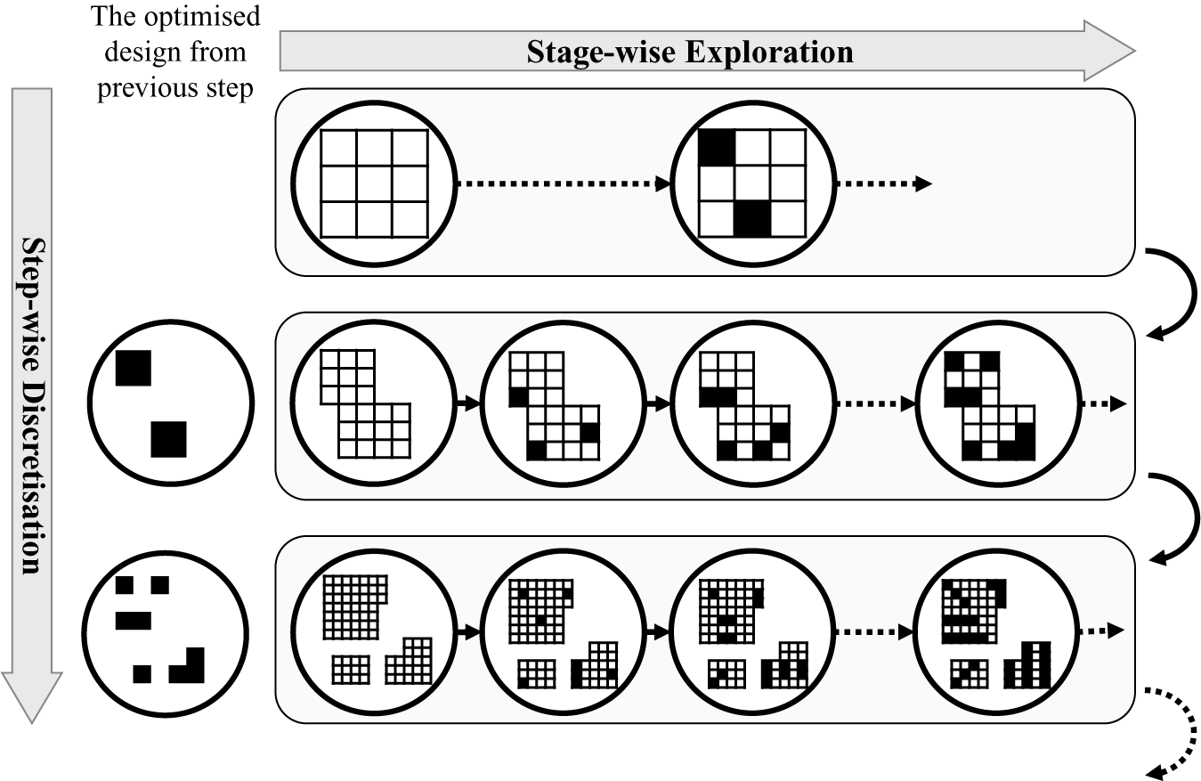
The schematic design space for a component is shown in Figure 2. For a faster convergence, the initial screening stages during the optimisation process can be done by a coarsely discretised design space over the whole physical design space of a component, as in Figure 2a. After the significant patches are identified in the first stage, the design space can be discretised with finer patches. This will help to identify the local geometrical features with a higher resolution. As shown in Figure 2b, the design space at this stage includes the identified patches from the previous stage (Figure 2a) with a finer discretisation. The design space at this stage includes the neighbouring area to the optimised form from the previous stage as well. Similarly, the design space in Figure 2c involves the optimised form from the previous stage, Figure 2b, with a finer discretisation and by adding the neighbouring patches. Despite a finer resolution in later stages, the total area concerning the added thickness can be controlled to remain equivalent in all stages. The process continues at each stage by redefining the design domain and introducing finer discretised patches. Discretisation steps can be continued until a satisfactory resolution is achieved for the optimised form by considering the design prerequisites and the available computational resources.
The stepwise design space discretisation for topometry optimisation, (a) discretised design space at step 1, (b) discretised design space at step 2, (c) discretised design space at step 3

Stage-wise exploration
At each step of the optimisation process, a design space exploration is done by the optimisation algorithm to identify the most significant patches concerning the optimisation objectives, which in this work were the S&R risk metrics. Depending on the availability of computational resources, the exploration can be done at different stages. If the goal with the optimisation is to find geometrical patterns with an added mass of md, the optimisation process at each discretisation step can be divided into n, stages. At each stage, the allowable added mass can be a fraction of md, or md/n in case of an even distribution among the stages. To meet the design and manufacturing considerations, the progression of the geometrical pattern can be controlled by some rules. This can be done by identifying some projection directions during the optimisation stages, or by avoiding scattered patterns by introducing proximity constraints to form clusters of patches, or if design constraints impose the inclusion or exclusion of certain features, such as feature angles or width and height dimensions. Accordingly, the proximity constraint was employed in this work to achieve a proper representation of the reinforcement areas. The proximity constraint was defined based on the Euclidean distance between the patches in the design space similar to Mozumder et al. (Reference Mozumder, Renaud and Tovar2012). Consider the results of the first stage of the optimisation for a schematic design space as shown in Figure 3a by solid black patches. In the second stage of optimisation, the performance of the patches is penalised based on the proximity factor. xi op and yi op refer to the coordinates of the ith optimised patch in a stage as shown in Figure 3a. The proximity of the jth patch belonging to the design space at the second stage with centre coordinates of xjp and yjp is calculated as
 $$ {P}_d=\sqrt{{\left({x}_{\mathrm{op}}^i-{x}_p^j\right)}^2+{\left({y}_{\mathrm{op}}^i-{y}_p^j\right)}^2.} $$
The stage-wise exploration and the proximity constraint, (a) design space exploration at stage 1, (b) design space exploration at stage 2, (c) design space exploration at stage 3.

The patches with a proximity distance equal to the average length of the patches in the design space form the first neighbouring layer around the optimised patches from the previous stage, as shown by dark green patches in Figure 3a. The performance results of these patches are not penalised. The patches with a proximity distance of twice the patch length belong to the second layer of the neighbouring patches and are shown by light green patches in Figure 3a. The calculated performance for these patches is 50% penalised. The patches located beyond the second neighbouring layer are excluded from the design space at each stage. Consider the optimised form of the component at the end of the second stage as shown in Figure 3b, with the newly added patches to the geometrical form by red squares. Accordingly, the design space for the next stage would consist of the first and second neighbouring layers around the optimised form from the previous stages as given in Figure 3c. To further enhance the integrity and concentration of the reinforcements, an additional constraint was introduced in the optimisation process. The constraint limits the involvement of the designs with several patches in the second neighbouring layer. So, in the industrial application that is presented in this article, a design was considered feasible if at least 50% of the modified patches in the respected stage were in the first neighbouring layer.
The proposed stage-wise exploration procedure introduced in this work has some advantages compared to a single-stage optimisation. The introduction of the proximity constraint confines the design space and accelerates the exploration process. The proximity constraint can be further elaborated by introducing other manufacturing constraints such as directionality or transition slopes among the patches resulting in better realisable solutions. The flexibility in interrupting the optimisation process at earlier stages if satisfactory designs are achieved reduce the total mass. The addition of discretisation steps and exploration stages provides proper controllability over the whole optimisation process. Further, these all can result in a computationally affordable topometry optimisation process. However, as a drawback, the introduction of discretisation steps and exploration stages might add to the complexity of the problem setup and demands extra effort in preprocessing the optimisation models. But the reduced optimisation process in large problems can overweigh the required preprocessing effort.
4.2. Optimisation approach
Since the problem at hand aims to reduce the risk for the generation of S&R by observing metrics from different disciplines, geometric variation and dynamic behaviour, a multiobjective optimisation approach (MOA) is required to be employed. Ölvander reviewed the MOA methods that have been frequently referred to within the engineering design context (Ölvander Reference Ölvander2000). The optimisation problem dealt with in this article is a high dimensional problem as it involves many input variables and field variables connected to several DOFs in the FE model. As the problem is formulated, it forms a discontinuous problem involving FE models to estimate the system response. The high complexity and dimension levels turn the problem into a multimodal problem with several possible local optima. The high dimension, multimodality and discontinuity of the problem make the use of deterministic optimisation approaches unsuitable (Coello, Lamont & Van Veldhuisen Reference Coello, Lamont and Van Veldhuisen2007). Also, S&R is caused by stochastic dynamic vibrations. Therefore, evolutionary algorithms that are mostly based on stochastic processes in nature could be suitable approaches to be employed for the problem at hand. Genetic algorithm (GA) has been widely used in engineering problems as an evolutionary optimisation method (Goldberg Reference Goldberg1989), which was inspired by Darwin’s theory of ‘survival of the fittest’. Multi-Objective Genetic Algorithm (MOGA), as introduced by Fonseca & Fleming (Reference Fonseca and Fleming1993) was used in this study as the optimisation approach. MOGA enables a proper global search and avoids trapping in local optima if the problem is properly formulated. However, it might come at a high computational cost. But, unlike deterministic optimisation methods, if the evolutionary approaches are implemented suitably, they can always lead to good solutions when achieving the real optimum becomes expensive because of a costly thorough global search. MOGA algorithm is based on evolving designs at sequential generations that are generated from elite parents from the previous generations. For this purpose, the fittest designs are selected based on their domination rank (Goldberg Reference Goldberg1989) and stored in an elite pool (Fonseca & Fleming Reference Fonseca and Fleming1993; Coello et al. Reference Coello, Lamont and Van Veldhuisen2007). The MOGA algorithm is described in Poles (Reference Poles2003) and Coello et al. (Reference Coello, Lamont and Van Veldhuisen2007).
The thickness optimisation workflow utilised in this work consists of different layers of discretisation and exploration, as depicted in Figure 4. The optimisation starts with a coarse discretisation of the design space, forming the first step of the optimisation process. Then, by a manual setting, the optimised thickness distribution can be obtained through single or multiple stages of optimisation as described in Section 4.1.2. In the case of multiple stages, at each stage, a percentage of the target added mass can be distributed by varying the shell thickness of the discretised element patches. The exploration stages can be continued until designs with satisfactory objective values are attained or the target added mass is reached. The optimised design from the first step would then be used to determine the boundaries for the initial design space for the next step. The design space is discretised by a finer resolution that in addition to the patches with varied thickness from the previous stage includes the first neighbouring patches to them. The thickness of all the patches is reset to the baseline value at the start of each discretisation step. Again, the optimised distribution of the patches can be determined through a stage-wise exploration considering the design objectives and mass constraints. The discretisation steps can be continued until the required level of details for the stiffening features is identified. Another determining factor for stopping the optimisation process is the available time and simulation resources.
The high-level flowchart of the thickness optimisation workflow consisting of discretisation and exploration layers.
In order to identify the best design solutions in every exploration stage in a discretisation step, the MOGA optimisation method was used in this work as explained earlier. The workflow of the deployed optimisation approach is given in the flowchart of Figure 5. The optimisation process starts with the first population, which in this work was defined as a DOE table generated using the incremental space-filling algorithm (Pronzato & Müller Reference Pronzato and Müller2012; Fang et al. Reference Fang, Liu, Qin and Zhou2018). The utilised algorithm can be found in Bayani et al. (Reference Bayani, Wickman, Lindkvist and Söderberg2022 b). Next, the designs in a population are checked for the problem constraints, being the proximity constraint and the sorting constraint. The proximity constraint is discussed in Section 4.1.2 and the sorting constraint is explained in Section 5.2. Each of the feasible designs is then evaluated in terms of the objective functions. For this purpose, the thickness of the shell elements in the FE models used for the geometric variation analysis and structural dynamics analysis is updated respecting the thickness variables in each design. A script was used to automatically rewrite the bulk data file of the FE models by modifying the thickness values. Then, the virtual simulations are executed. For geometric variation, the variation and deviation metrics were output from the RD&T software. For dynamic response, the frequency response of the system at the measure points and the modal vectors of the FE model in the DOFs of the measure points were calculated by NASTRAN 111 and 103 solvers. The objective functions introduced in Eqs. (3) and (8) were then calculated from the simulation results using a scripted process. Next, the fitness level of every design is determined by calculating its domination factor in the MOGA approach (Goldberg Reference Goldberg1989). Designs belonging to the Pareto front are then nominated to update the elite pool that contains the best performing designs during the optimisation process. By utilising GA operators, which are mentioned in Section 5.2 for the industrial case, the next generation of the designs is created. The optimisation process can be manually interrupted when a saturation state is observed among the Pareto designs, or when satisfactory objective values are achieved, or when the calculation resource limitations impose a termination.
The employed optimisation flowchart (based on the MOGA) for optimising the thickness distribution.

5. Industrial application
The proposed stage-wise optimisation approach with proximity constraints was used in some industrial as well as generic cases. In this article, a problem with industrial complexity and applicability is presented. For the generic geometry, consisting of a simpler model, see Tang & Lindkvist (Reference Tang and Lindkvist2021). The optimisation aimed to find the patches with the highest impact on improving the system behaviour in terms of design robustness and structural dynamic properties to minimise the risk for the occurrence of S&R.
5.1. FE modelling and design space discretisation
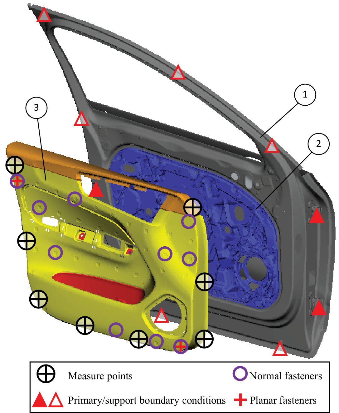
The industrial problem involved the side door assembly of a passenger car. The FE model of the side door is depicted in Figure 6. The model involves three main subassemblies of (1) the door structure, (2) the door module and (3) the inner door panel. The FE model details and material information are given in Table 1. In the presented work in this article, the most effective areas in the inner door panel part for adding stiffener patterns were identified. In a previous study (Krishnaswamy & Sathappan Reference Krishnaswamy and Sathappan2020), the connection configuration to mount the inner door panel to the rest of the door assembly was determined using the objective metrics introduced in Eqs. (3) and (8). The positions of the normal and planar fasteners between the inner door panel and the door, as defined in this work, are marked by purple circles in Figure 6. In the dynamic solver, Nastran, the fasteners were modelled by stiff linear springs, CBUSH elements.
Finite element model of the side door assembly: (1) door structure, (2) door module and (3) inner door panel.
Finite element model information

a Acrylonitrile butadiene styrene;
b Polypropylene;
c Reinforced polypropylene Hostacom T20.
For the geometric variation simulation in RD&T, the fasteners were modelled by rigid normal and in-plane fasteners. The system response was measured at eight measure points as shown in Figure 6. For the dynamic response metric, the relative motion between every measurement node pair was output in the rattle direction and the squeak plane as shown in Figure 1. In the geometric variation analysis, gap measurements in the rattle direction and the squeak plane in the measure points were statistically calculated. The boundary conditions of the model were defined based on the mounting interfaces between the door and the car body. The positions of the lock and the hinges were considered as the primary boundary conditions and were constrained by clamp joints in dynamic response analysis. These points were used as the fixed points in the positioning system using the 3–2–1 principle in geometric variation analysis. Additionally, the normal direction degree of freedom was constrained in seven support points in both simulations to replicate the door rubber sealing restraining effect.
5.2. Optimisation setup
The optimisation method in this work was MOGA as briefly introduced in Section 4.2. The GA operators used were directional and classical cross-over, selection and mutation with the assigned probability factors of 50, 35, 5 and 10%, respectively. The selection of an operator was done by a randomly generated number and based on the assigned probability factor for each operator as described in Bayani et al. (Reference Bayani, Wickman, Lindkvist and Söderberg2022 b).
The optimisation was conducted in two steps with different discretisation resolutions. The first step involved a sensitivity analysis to determine the important areas of the design space. The second step consisted of three optimisation stages to identify a geometrical pattern to add the structural stiffeners. The first generation of the designs in every optimisation stage was generated by an incremental space-filling method (Pronzato & Müller Reference Pronzato and Müller2012; Fang et al. Reference Fang, Liu, Qin and Zhou2018). The population size, number of generations and the parameter variation levels of the design variables are given in Table 2. The driving factors in setting these numbers were primarily the available computational resources. In the MOGA procedure, different orders of the variables representing the modified patches result in different designs. However, for the problem at hand, they were considered identical as the order of the thickness variation did not influence the system response. Thus, the repeated designs with different variable orders were excluded from the evaluation by using a sorting constraint. The objective functions to be minimised were the metrics introduced in Eqs. (3) and (8) with the weighting coefficients of α GV = 79 and α DR = 86. These weighting coefficients were defined based on the variation ranges for the metrics in each of the objectives and by considering equal importance for them. The variation ranges were defined by referring to the results of an initial DOE study of the model.
Optimisation variables, population, mass targets at each stage

5.3. Sensitivity analysis to confine the initial design space
Design space exploration in the first step of the optimisation process with a coarse discretisation can be done by a sensitivity analysis. In this study, different sensitivity analysis methods were tried for this purpose and the best performing method was chosen by monitoring the R-squared values, considering the capability of capturing the interdependencies among the variables and the efficiency of the method. The Plackett–Burman design with fold-over (Montgomery Reference Montgomery2012) was used to estimate the effect of each variable variation on the system response. The design of experiments (DOE) table for the Plackett–Burman with fold-over is constructed by adding a fold-over to the DOE table of the Plackett–Burman. A fold-over design is obtained by reversing the signs of all the variable variations in a DOE table. This increases the accuracy of the analysis by capturing the two-factor interaction effects in addition to the main effects (Montgomery Reference Montgomery2012). The Plackett–Burman DOE is a two-level fractional factorial design that can give an estimation of the main effects of the variables with a limited number of evaluation steps. The patches were ranked based on their effect estimates calculated from the Plackett–Burman with fold-over DOE results. The effect estimate Ev for a design variable vi from the DOE table was calculated as the difference between the average objective function value for the designs with high-level vi and the designs with low-level vi as
 $$ {E}_{v_i}=\frac{1}{d_{h,i}}\sum \limits_{j=1}^{d_{h,i}}{F}_{\mathrm{obj}}\left({D}_j\right)-\frac{1}{d_{l,i}}\sum \limits_{j=1}^{d_{l,i}}{F}_{\mathrm{obj}}\left({D}_j\right). $$
dh,i and dl,i are the number of designs in which variable vi gets the high- and low-level values, respectively. F obj(Dj) is the objective value calculated from Eqs. (3) and (8) for the design Dj from the DOE table. The relative effect estimate Ēv for a design variable vi was calculated relative to the baseline design, D nom, where all patches had the nominal low-level thickness.
 $$ {\overline{E}}_{v_i}=\frac{E_{v_i}-{F}_{\mathrm{obj}}\left({D}_{\mathrm{nom}}\right)}{F_{\mathrm{obj}}\left({D}_{\mathrm{nom}}\right)}. $$
The highly ranked patches based on the estimated effects were selected as the most effective variables concerning the objective functions. Since the problem at hand was a multidisciplinary problem with objective functions reflecting the design robustness and the dynamic response of the system, a combined threshold check was required. Therefore, the normalised effect estimates concerning each objective function were calculated to enable a balanced comparison of the design robustness and the dynamic response effect estimates as
 $$ {{\hat{E}}_{v_i}}^{\mathrm{GV}}=\frac{1}{{e_p}^{\mathrm{GV}}}\sum \limits_{j=1}^{{e_p}^{\mathrm{GV}}}{{\overline{E}}_{v_j}}^{\mathrm{GV}},\hskip0.35em {{\hat{E}}_{v_i}}^{\mathrm{DR}}=\frac{1}{{e_p}^{\mathrm{DR}}}\sum \limits_{j=1}^{{e_p}^{\mathrm{DR}}}{{\overline{E}}_{v_j}}^{\mathrm{DR}}. $$
ep GV and ep DR are the numbers of relative effect estimates Ēv that have positive values for geometric variation metric and dynamic response metric, respectively.
6. Results and discussion
6.1. The sensitivity analysis in the first step of the discretisation
In the first step, a coarsely discretised stating design space with 56 patches of 100 × 100 mm was used. The nominal thickness of the patches was 1.8 mm. In the sensitivity analysis study, the high-level thickness was considered 2.1 mm. The normalised effect estimates respecting the geometric variation metric and the dynamic response metric, Eq. (10), were calculated based on the two-level Plackett–Burman with fold-over DOE table with 120 designs. The results are presented in the bar chart in Figure 7. The results are sorted based on the aggregated effect values, with the most effective patches staying on the left side. The mean value of the positive normalised effect estimates for the geometric variation metric and the dynamic response metric is shown by the dashed grey line and the solid black line, respectively.
The sensitivity analysis results in the first step of the design space discretisation.

All patches with positive effect estimate that at least one of the normalised effect estimates for geometric variation or dynamic response was above the mean lines were selected as the design space for the next step of the optimisation. These patches are highlighted with a grey shading in Figure 8a and marked by red squares around the patch number labels in Figure 7. To comply with the engineering design guidelines for subsystem assemblies in passenger cars, the patches containing the fasteners were also added to the design space for the second step of the optimisation process as shown in Figure 8b.
(a) The patches with the highest effect estimates in the first step and (b) the initial design space for the second step of the design discretisation.

6.2. The second step of the optimisation process with a finer discretisation
The FE model for the second step of the optimisation was discretised by 180 finer patches with a size of about 60% of the first step as depicted in Figure 8b. The design space in the first stage included the identified effective patches from the sensitivity analysis plus the areas around the fasteners. It was assumed that an increase of about 3% in the part mass was permissible. Another alternative approach could be to reduce the overall thickness of the part by 3% and then allocate the saved mass for the optimisation problem. Considering the computational resources, available time and required design complexity, the optimisation problem was decided to be divided into three phases, with about a 1% increase of mass at each stage. The number of modified patches was decided to be 11 with an increase of 0.3 mm in thickness, accounting for 6% of the area of the inner door panel. The initial and the added thickness of the shell elements, the number of variables, the population size, the number of generations and the added mass at each stage are summarised in Table 2.
The first stage of the second step of the optimisation process involved 20 generations. The scatter plot of the evaluated designs in the first stage is depicted in Figure 9 by green squares with the lightest shade. The Pareto designs of the first stage are marked by yellow circles in Figure 9. The thickness distribution for the selected designs from the Pareto front in each stage, as given in Figure 9, is presented in Figure 10. The first row (α) in Figure 10, shows the designs with balanced objective metrics for geometric variation and dynamic response. In the second row (β), the designs from the Pareto fronts with the best dynamic response objective values are given. The designs with the best performance in terms of the geometric variation objective are shown in the lower row (γ). Pareto designs belonging to stages one to three are presented in columns (a) to (c) in Figure 10, respectively. A design from the Pareto front with balanced objective values, ‘Opt stage 1’, was chosen to construct the design space for the second stage. The resultant thickness distribution for this design is shown in Figure 10(a – α).
The scatter plot of the objective values for different designs in the optimisation process.

The schematic thickness variation for (a–c) the results at different optimisation stages, (α) the selected designs at each stage as the optimised design and (β–γ) in selected designs from the Pareto front in Figure 9.

The design space of the second stage of the optimisation included the modified patches in stage one and their first and second neighbouring patches. In addition to the neighbouring patches, it was permissible to opt the patch candidates for thickness modification from the already modified patches in stage one to allow the accumulation of more material where required. The scatter plot of the evaluated designs of the second phase is shown in Figure 9 by green squares with neutral shading and the Pareto designs are marked by orange circles. Similar to the previous stage, the design labelled ‘Opt stage 2’ with balanced objective values was used to construct the design space for the third phase of the optimisation. The thickness distribution for ‘Opt stage 2’ is shown in Figure 10(b, – α). Among the modified patches, four were already modified in the first stage and got a thickness value of 2.4 mm. The scatter plot of the third phase is given with darkly shaded green squares in Figure 9 with the Pareto fronts highlighted by red circles.
In stage three, the design with the best dynamic response metric (c – β) had a more distributed thickness pattern compared to the design with the best geometric variation metric (c – γ) that consisted of more concentrated reinforcements. In the second stage, however, both designs with the best objective metrics (b – β and b – γ) had similar thickness concentrations. The designs with the best dynamic response metric in all stages (β) more tend to involve the upper patches than the designs with the best geometric variation metric (γ). Nevertheless, the patches in the lower right corner are more included in the designs with good performance in terms of the dynamic response in the first and third stages (a – β and c – β).
6.3. The optimised thickness distribution for the side door inner panel
Selecting the optimised thickness distribution for the industrial case at hand can be done by considering weightings for the engaged objective functions: the geometric variation and dynamic response metrics. Indeed, this decision should be done by the design team considering the other contributing design objectives and attributes. By referring to the Pareto designs shown in Figure 9 and by considering a balanced and even weighting for both of the objective metrics, a Pareto design from the third stage like the one labelled by ‘Opt stage 3’ in Figure 9 could be considered as a possible optimum solution. The thickness distribution of the selected optimum design, ‘Opt stage 3’, is shown in Figure 10(c – α). The resulted pattern included a uniform part with 1.8 mm thickness with six 2.1-mm-thick, two 2.4-mm-thick, and three 2.7-mm-thick stiffening patches, as shown in Figure 10(c – α). Most of the reinforced patches clustered around the fasteners or close to them except the patch located at the lower-left corner of the inner panel. Also, the areas around the upper-right fastener remained unchanged. The calculated objective metrics for the baseline design, with the baseline thickness distribution of 2.1 mm, is shown by a cross in Figure 9. Compared to the baseline design the calculated objective values for the selected optimised design, ‘Opt stage 3’, improved from 8.98 to 8.89 mm for the geometric variation metric and from 32,250 to 27,100 for the dynamic response metric.
To verify the performance of the optimised design, the system response of the side door assembly when excited by a time-history road disturbance was calculated. The excitation signal was a synthesised time-history signal based on the measured vibrations at the mounting interfaces of the side door while the complete vehicle was driven on a Belgian Pave surface at the proving ground, see Bayani et al. (Reference Bayani, Nilsson, Blom, Wickman and Söderberg2021) for details. The boundary conditions of the FE model were defined as shown in Figure 6 and the excitation was applied as imposed acceleration at the locations of the hinges (the solid red triangles on the right side of the door assembly in Figure 6). The system response was calculated at the same measure points shown in Figure 6 by solving the transient response of the system using the NASTRAN modal transient solver (SOL 112). The system response was calculated in terms of the relative normal displacement between the door panel and the door structure, as well as the S&R severity metrics given in Eqs. (5) and (6). The results of the system with the optimised thickness design are compared with the baseline design with a uniform thickness distribution in Figure 11. The relative displacement and the severity metrics are given for the top-left measure point and the bottom-right measure point of the side door inner panel in Figure 11a,b, respectively. For better illustration, the negative displacement data points, indicating an increase in the interface clearance are not shown in the results. In both measure points, the results show that the introduction of the optimised thickness distribution resulted in the reduction of the relative displacement between parts. Similarly, by referring to the calculated S&R severity metrics in Figure 11, a reduction in the risk for S&R is expected for the optimised design as compared to the baseline design.
Relative displacement and squeak and rattle severity factors for the baseline and optimised designs excited by Pave disturbance at the (a) top-left measure point and (b) bottom-right measure point of the inner door panel.

6.4. Reflection on the effectiveness of the proposed thickness optimisation approach
The improvement made in the dynamic response objective metric in this work proved that thickness optimisation can be as effective as optimising the connection configuration in an assembly for reducing the S&R risk, which was done previously (Krishnaswamy & Sathappan Reference Krishnaswamy and Sathappan2020; Bayani et al. Reference Bayani, Wickman, Krishnaswamy, Sathappan and Söderberg2022 a). However, by looking at the achieved improvement for the geometric variation objective metric in this work and by comparing it with the improvement gained in previous works by optimising the connection configuration (Krishnaswamy & Sathappan Reference Krishnaswamy and Sathappan2020; Bayani et al. Reference Bayani, Wickman, Lindkvist and Söderberg2022 b), it could be argued that thickness optimisation is less effective for improving the design robustness in an assembly compared to the connection configuration optimisation. But the concentration of the stiffeners in the vicinity of the fasteners implies the dependence of the topometry optimisation results on the connection configuration in an assembly. Therefore, it is expected that by a coupled multidisciplinary optimisation, in which design parameters involve the location of the fasteners as well as the distribution of the stiffeners (or part thickness), the contribution of the geometric variation objectives in determining the thickness distribution to minimise S&R risk could increase.
By referring to the scatter plot in Figure 9, it can be seen that all Pareto designs in all stages, except Pareto1_1 in stage one, outperformed the baseline design. Nevertheless, the existence of designs with poorer performance respecting one or both optimisation objective metrics denotes the necessity of using a proper structural modification method to introduce stiffening patterns in parts. In addition, the evaluated designs with enhanced performance in one objective metric and deterioration in the other stress the need for a coupled optimisation process for thickness distribution by involving the geometric variation metrics and structural dynamic metrics in a multidisciplinary approach. Indeed, in the case of decoupled optimisation, achieving designs with improved performance in both disciplines would be harder. For instance, one could consider Pareto1_1 in stage one as an optimum solution in a single dynamic response optimisation problem while the robustness of this design is lower when compared to the baseline design.
7. Conclusions
In this article, a stepwise topometry optimisation approach was proposed to involve robust design in closed-loop structural modifications to reduce the risk for S&R events. The proposed method involved a stepwise design space discretisation and a stage-wise design domain exploration with the aid of the multiobjective GA optimisation method. The design domain confinement as a result of the stage-wise exploration and stepwise discretisation, the flexibility and controllability in the problem formulation and the optimisation process and the implementation of shape control constraints such as proximity resulted in an accelerated and affordable optimisation method. The proposed method was used in a multiobjective problem to find the stiffener patterns by modifying the thickness distribution in the inner door panel of a passenger car to reduce the risk for the generation of S&R. The optimisation objectives were formulated by utilising quantified metrics to estimate the contribution of design robustness and dynamic behaviour of the system to S&R risk severity. For this purpose, statistical measures computed from the geometric variation analysis and resonance risk and mode shape similarity indicators computed from the frequency response of the system at critical interfaces for S&R were employed. The optimisation process resulted in designs outperforming the baseline design by reducing the risk of S&R. However, the existence of structurally modified designs without a performance improvement among the population designs signifies the need for a closed-loop structural design approach to add stiffness to a part. Expectedly, most of the material was added in the vicinity of the fasteners where higher stress concentration might exist.
The application of the proposed topometry optimisation procedure in the industrial case in this work was done by some assumptions. Nevertheless, some problem formulation details could be set alternatively. These alternative settings may lead to further work and studies that will be mentioned here. The thickness variation was always assumed to increase material in a patch, while it is possible to allow thickness reduction as well. This way, the spared material from a patch can be distributed to other patches to minimise the total mass. The proximity constraint used in this work can be accompanied by other manufacturing constraints like the growth direction and thickness transition neighbourhoods. Design space discretisation can be done with finer resolutions and more exploration stages can be involved to achieve a better design realisation. A study can be conducted on the efficiency of the method by varying the number of exploration stages and the included variables at each stage. The proposed topometry method was used to optimise the thickness distribution of a component in an assembly with a predetermined connection configuration. An interesting study might be to use the proposed topometry optimisation approach together with the methods introduced in Bayani et al. (Reference Bayani, Wickman, Krishnaswamy, Sathappan and Söderberg2022 a,b) to define optimised connection configurations in a concurrent multidisciplinary optimisation problem.
To summarise, in this work a topometry optimisation procedure was proposed that uses the multiobjective GA to distribute thickness in thin panels. The introduced stepwise discretisation and stage-wise exploration can accelerate the optimisation process for reducing the risk for S&R in large assemblies by objectively analysing the design robustness and the frequency response of the system. This might facilitate the involvement of geometric variation analysis in structural optimisation together with other virtual simulations. Ultimately, by utilising this approach the risk for the generation of the S&R can be reduced by proper use of the material in increasing the stiffness in components and assemblies.
Financial support
This work was funded by Volvo Car Corporation and was done in collaboration with Wingquist Laboratory at Chalmers University of Technology and Lund University.


 Open access