


1. Introduction
Glacier volume and ice thickness distribution are highly important for various aspects of glaciology, as well as for related sciences, such as hydrology (e.g. IPCC, 2013; Bahr and others, Reference Bahr, Pfeffer and Kaser2015). Ice thickness is a key factor determining the flow of glaciers, the potential water volume contributing to local and regional runoff, and the amount of sea-level rise due to glacier wastage during climate change. However, even with the great efforts expended into conducting ice thickness measurements with geophysical methods, these direct observations remain sparse (Gärtner-Roer and others, Reference Gärtner-Roer2014; GlaThiDa-Cons, 2019). It is therefore imperative to be able to infer ice volume and thickness distribution of large glacier samples from readily available data, such as glacier inventories and digital elevation models (DEMs). The development of approaches capable of estimating ice thickness has recently become a relevant branch of glaciological research and various models of different complexity and input data requirements have been proposed (see Farinotti and others, Reference Farinotti2017, for a review). The Ice Thickness Models Intercomparison eXperiment (ITMIX) compared the performance of 17 different approaches for a standardised set of glaciers (Farinotti and others, Reference Farinotti2017). Considerable differences were found in the skill of the individual models to reproduce point ice thickness observations but even the best approaches were subject to large errors. This indicates a pressing need to further develop the corresponding approaches.
The archetypal ice volume estimation technique is volume-area scaling (e.g. Chen and Ohmura, Reference Chen and Ohmura1990; Bahr and others, Reference Bahr, Meier and Peckham1997; Grinsted, Reference Grinsted2013; Bahr and others, Reference Bahr, Pfeffer and Kaser2015) which relates ice volume to glacier area through a power law, for which the exponent is well constrained by theory. This approach is both robust and straightforward but is unable to account for the characteristics of individual glaciers, and does not deliver spatially distributed ice thickness. The latter strongly limits the method's applicability to modern glaciological studies as bedrock topography is a requirement for physical models of ice flow, subglacial hydrology, transient glacier retreat, future hydrology, etc. Furthermore, the validation of average ice thicknesses estimated by volume-area scaling is inherently difficult as they cannot directly be compared to point-based thickness measurements.
Models simulating ice thickness distribution typically rely on the principles of ice-flow dynamics. Some approaches are based on the assumption of constant basal shear stress along a central flowline (e.g. Li and others, Reference Li, Ng, Li, Qin and Cheng2012; Frey and others, Reference Frey2014; Linsbauer and others, Reference Linsbauer, Paul and Haeberli2012). An important group of models hinges on considerations of mass conservation (in a reduced, one-dimensional geometry) paired with ice physics (e.g. Farinotti and others, Reference Farinotti, Huss, Bauder, Funk and Truffer2009; Huss and Farinotti, Reference Huss and Farinotti2012; Clarke and others, Reference Clarke2013; Langhammer and others, Reference Langhammer, Grab, Bauder and Maurer2019; Maussion and others, Reference Maussion2019). The other important group of models makes use of observed ice velocities within a two-dimensional, mass-conservation equation to infer ice thickness (e.g. Morlighem and others, Reference Morlighem2011; McNabb and others, Reference McNabb2012; Gantayat and others, Reference Gantayat, Kulkarni and Srinivasan2014; Brinkerhoff and others, Reference Brinkerhoff, Aschwanden and Truffer2016; Fürst and others, Reference Fürst2017). Other ice thickness models propose the inversion of full ice-dynamics models (Van Pelt and others, Reference Van Pelt2013), or are based on neural networks (Clarke and others, Reference Clarke, Berthier, Schoof and Jarosch2009).
Many approaches have been designed to infer the ice thickness distribution of individual glaciers, other have the goal of being applicable on a regional to global scale. Within the Global Glacier Thickness Initiative (G2TI) (Farinotti and others, Reference Farinotti2019) up to five ice thickness models have been applied globally resulting in a consensus estimate relative to the version 6.0 of the Randolph Glacier Inventory (RGI) (RGI-Consortium, 2017).
With the rapid progress in satellite-based Earth observation, new large-scale datasets are becoming available at a fast pace. Most global ice thickness models to date have relied on surface topography and glacier inventories only. However, there is considerable potential in including information contained in ice velocity, expected to soon become available globally from satellite products (e.g. Fahnestock and others, Reference Fahnestock2016; Mouginot and others, Reference Mouginot, Rignot, Scheuchl and Millan2017; Strozzi and others, Reference Strozzi, Paul, Wiesmann, Schellenberger and Kääb2017; Gardner and others, Reference Gardner2018; Dehecq and others, Reference Dehecq2019a). Furthermore, the optimal inclusion of direct ice thickness observations via inversion techniques is a highly important aspect as the number of these observations is increasing rapidly.
Inversion schemes, taking into account as much of the available information as possible, are thus required. Of interest here is the publication by Brinkerhoff and others (Reference Brinkerhoff, Aschwanden and Truffer2016) as it employs a Bayesian inference method. Such methods allow combining prior knowledge of the system with the fitting of a physical model to observations. Furthermore, within such a framework, numerical schemes are available to not only find the best-fit parameters and predictions but to also compute their probability distributions, thus making this type of inversion particularly appealing. Regional- to global-scale applications and testing of such an approach, however, is still lacking.
Here, we present the Bayesian Ice Thickness Estimation model (BITE-model) which uses a novel, Bayesian approach making it applicable at large scales. We considerably enhance an extensively tested forward model for inferring ice thickness and volume based on mass flux estimates (Huss and Farinotti, Reference Huss and Farinotti2012). Furthermore, we use comprehensive datasets of surface ice speed, surface mass balance and elevation change, and a large sample of direct ice thickness observations to apply Bayesian inference to produce maps of ice thickness, including explicit estimates of the uncertainty. The new approach is applied to glaciers and ice caps of regions containing either a very large ice volume (Svalbard, Arctic Canada), featuring a dense observational coverage (European Alps) or consisting of many diverse and large mountain glaciers (Karakoram). Results are compared with the recent G2TI estimates of regional glacier ice volume.
2. Methods
The BITE-model consists of: (i) a forward model, which is a mass-conserving, ice-physics-inspired ice thickness model based on Farinotti and others (Reference Farinotti, Huss, Bauder, Funk and Truffer2009) and Huss and Farinotti (Reference Huss and Farinotti2012); and (ii) an inverse model which uses Bayesian inference, taking into account both prior knowledge and available measurements of the system.
2.1 Forward model
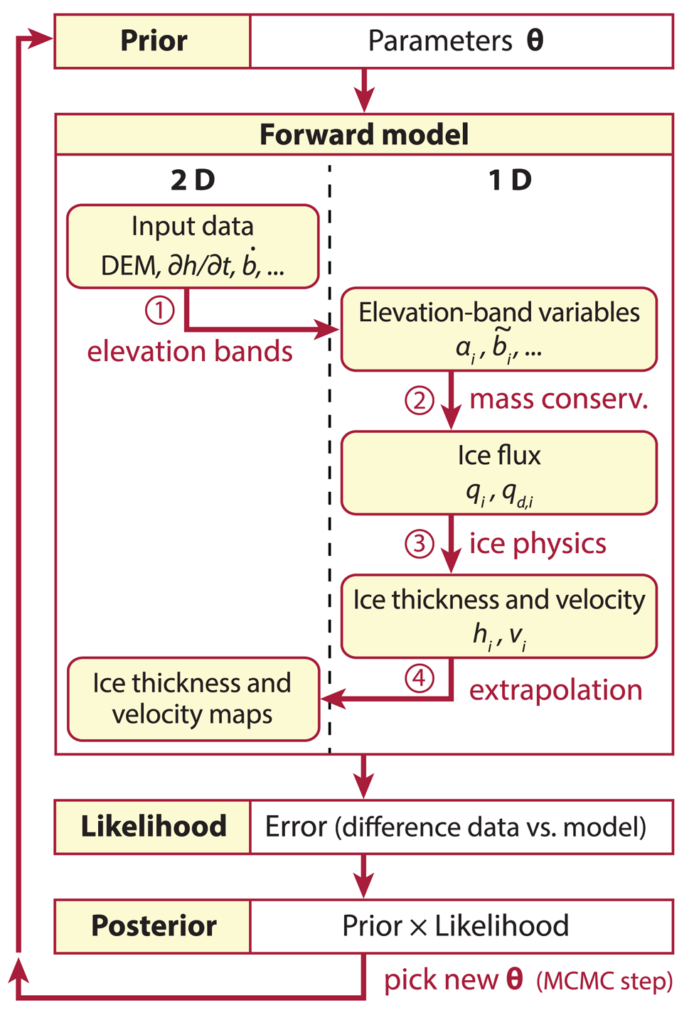
The forward model computes an ice thickness and surface ice speed map for given input maps and parameters. It is a re-implementation and further development of Huss and Farinotti (Reference Huss and Farinotti2012) and uses a mass-conservation approach combined with ice-flow physics as given by the shallow ice approximation. The model complexity as well as its computational cost is reduced considerably by performing most calculations in one dimension (1D). The reduction to 1D is performed by binning all required data into elevation bands. This is similar to flow-line glacier models but using elevation-band averaged quantities, such as average thickness. The 1D thickness and surface ice speed are then extrapolated to obtain a spatial distribution of these variables. The forward model performs the following steps: (1) collapse the two-dimensional (2D) input data onto elevation bands, (2) calculate mass flux q through elevation bands, (3) calculate ice thickness h and surface ice speed v on elevation bands, and (4) extrapolate h and v to 2D. These steps are explained below in detail and are illustrated with an example run of Unteraar Glacier (Switzerland).
Schematic of the BITE-model. The forward model transforms input data (DEM, $\dot {b}\comma\; {\partial h}/{\partial t}$ , etc.) into output data (h,v), with the steps numbered as in the text. The inverse model (prior, likelihood and posterior) is evaluated using a Markov chain Monte Carlo (MCMC) scheme. For variable definitions, refer to Table 1 and Eqn (15).
Key input parameters and fields of the forward model which are used in the inversion and model output (last two parameters). The third column states whether the data need to be in 2D or whether a lower-dimensional input is possible. The last column indicates whether there are observations or model outputs available on a regional/global scale

2.1.1 Collapse onto elevation bands (step 1)
The original approach of this type of model (Farinotti and others, Reference Farinotti, Huss, Bauder, Funk and Truffer2009) required a manual selection of a flow line for each glacier sub-catchment. Huss and Farinotti (Reference Huss and Farinotti2012) simplified this approach by dividing the glacier into elevation bands and using elevation-band averaged quantities for the 1D calculation. The advantage of using elevation bands is that the collapse from 2D to 1D is straightforward to automate.
This is also the approach used here: The elevation range of the glacier is divided into N equal bands, each spanning an elevation difference of Δz = 30 m. Each cell of the DEM is then assigned to a band according to its elevation z. The area of each band a i is calculated by summing the areas of all cells in the band. Notice that this procedure discretises the problem and that the 1D equations we present below are inherently discrete. This is reflected in our notation: where 1D and 2D variables can be confused, we write the 1D variables with subscript ‘i’ indicating the elevation band, counted from the top (e.g. x i), and the 2D variables without subscript (e.g. x).
A representative slope angle for each band αi is needed for estimating the ice flow. This calculation is also critical as it will determine the horizontal length of an elevation band (see Eqn (1)) and hence the overall glacier length. We follow the empirical approach of Huss and Farinotti (Reference Huss and Farinotti2012) who take αi as the mean of all cell slopes over a certain quantile range: αi = mean{α′|Q 5(α) < α′ < Q x(α)} where x = min(max(2 Q 20(α)/Q 80(α), 0.55), 0.95) and Q x denotes the xth percentile. This approach removes outliers and returns a slope angle that is both representative of the main trunk of the glacier and consistent with its flowline length. Furthermore, we enforce 0.4° < αi < 60° (Huss and Farinotti, Reference Huss and Farinotti2014); the lower bound is to avoid infinities that ensue when the band length (Eqn (1)) becomes infinite and the driving stress (Eqn (7)) becomes zero. With αi, the length Δχi and width w i of each elevation band i can then be determined geometrically

Note that the glacier length in 1D is $l = \sum \Delta \chi _i$ and the corresponding horizontal coordinate in 1D is denoted by χ.
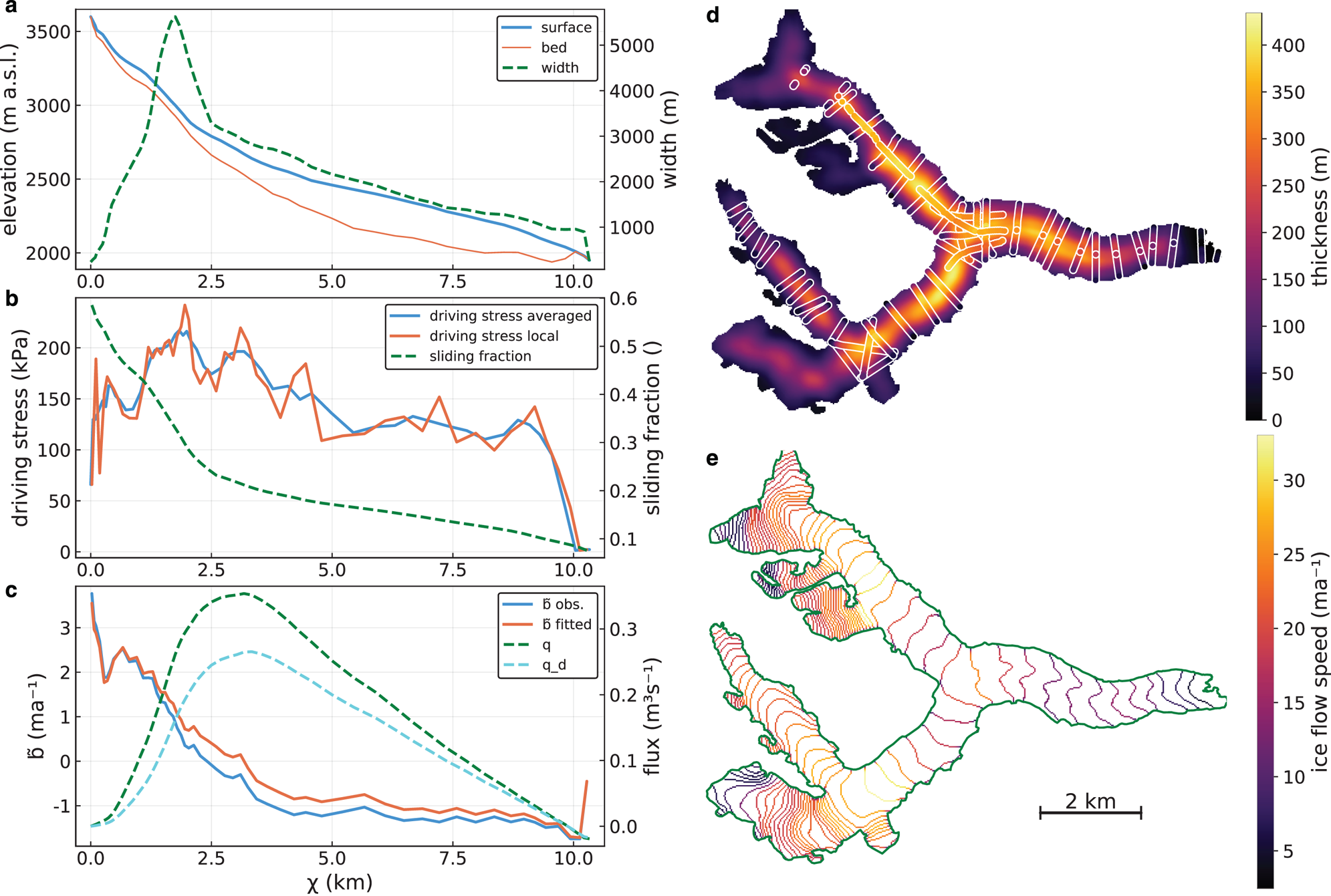
An example result of this procedure is given in Fig. 2a which shows the glacier surface and width in 1D against the horizontal elevation-band coordinate χ.
Best-fit forward model output for test case Unteraar Glacier (from ITMIX, Farinotti and others, Reference Farinotti2017), Switzerland. The left panels show 1D-model inputs and results, the right panels results extrapolated to 2D. (c) Glacier surface and bed elevation (left axis) and width (right axis); (b) driving stress (left axis) and basal sliding fraction f sl (right axis); (c) observed and fitted apparent mass balance $\tilde {b}$ (left axis), total flux q and deformational flux q d (right axis); (d) calculated ice thickness overlain by thickness along radar profiles (white-bordered); (e) surface ice speed at elevation-band boundaries.
2.1.2 Mass conservation (step 2)
The mass conservation equation in 1D (width and depth integrated, discretised on elevation bands) is given by

where q i is the flux from band i to i + 1, ∂h i/∂t is the rate of ice thickness change, and $\dot {b}_i$ is the mass balance (in metres ice per year). Defining the apparent mass balance $\tilde {b}$
 as
as

and summing the above equation gives

with boundary condition at the top q 0 = 0. Note that for land-terminating glaciers the flux is zero at the terminus q N = 0, whereas for calving glaciers q N > 0. Figure 2c illustrates the mass-balance terms and fluxes in 1D for the example glacier.
2.1.3 Ice thickness (step 3)
Ice thickness can now be calculated from the ice flux. For this, a partition of the flux due to internal deformation and due to sliding is required. Given the ratio of surface speed to basal sliding speed f sl, we can calculate the flux due to deformation as

with r = (n + 1)/(n + 2) = 0.8 the ratio between depth-averaged deformational flow speed and deformational surface flow speed (assuming shallow ice flow; n = 3 is Glen's exponent). Note however, that calculating f sl would require using a basal sliding law. We forgo this and will treat f sl as a tuning parameter.
The ice thickness h is then calculated from the deformational ice flux by using a formula derived from the shallow ice approximation (Cuffey and Paterson, Reference Cuffey and Paterson2010)

with A the temperature-dependent ice flow factor (for which we use the tabulated values of Cuffey and Paterson, Reference Cuffey and Paterson2010). The driving stress divided by the ice thickness $\tilde {\!\tau }$ is given by

where f i = w i/(2h i + w i) is a shape factor for a parabolic valley (Nye, Reference Nye1965). The above equation averages the local driving stress over 2k+1 elevation bands, with k chosen such that the horizontal extent is approximately six ice thicknesses. Kamb and Echelmeyer (Reference Kamb and Echelmeyer1986) recommend three to ten ice thicknesses for the averaging of τ. Figure 2b illustrates the averaged and local driving stress, as well as the employed basal sliding fraction f sl in 1D for the example glacier.
Ice thickness at ice divides is predicted to be zero by Eqn (6) as q d,0 = 0 and $\bar {\tau }\gt 0$ . Nonetheless, to account for the non-zero ice thickness found at those locations we set h 0 = h 1 for glaciers and ice caps originating at divides. Note that whilst this is at odds with the shallow ice formula (Eqn (6)) it is consistent with mass conservation (Eqn (2)) as flux is zero there.
The elevation-band depth-averaged ice speed is calculated using mass conservation as

which can be translated into a surface speed with

2.1.4 Extrapolation to the map plane (step 4)
The extrapolation of h (as calculated by Eqn (6)) to 2D is done such that the total volume $V = \sum _i h_i a_i$ is conserved. The ice volume of each band is distributed to the cells in 2D according to their surface slope and their distance L to the next land-margin of the glacier as

with the exponent 1 ≥ d > 0 being a tuning parameter, for which a value of 1 corresponds to a V-shaped bed and values closer to 0 to a more and more pronounced U-shape. The exponent of the sine term is given by the shallow ice approximation (Eqn (6)). In this equation, the minimum value of α is constrained to be 2.5° to avoid infinities (Huss and Farinotti, Reference Huss and Farinotti2014). The first factor of this formula is inspired by the shallow ice approximation from which also Eqn (6) is derived. For marine terminating glaciers, any ice thicknesses larger than flotation level are reduced to flotation. Finally, the resulting ice thickness field is smoothed with a moving average filter using a window-width of approximately the mean ice thickness (estimated by volume-area scaling). These last two steps are not strictly volume-conserving but the errors are very small in typical settings (Huss and Farinotti, Reference Huss and Farinotti2014 state that on the Antarctic Peninsula less than 1.8% of the area is affected by the former correction).
The extrapolation of the surface ice speed is mass conserving, which is an improvement on Huss and Farinotti (Reference Huss and Farinotti2012). We first assume that the depth-averaged ice speed $\bar {v}$ has a certain across-glacier distribution, namely that ice flows slower towards the margin and faster far from it. For this we use a formula inspired by Nye (Reference Nye1965) (his Eqn (6))

where the length scale λ = min(w i/2, h i) is the minimum of half-width and mean thickness and the exponent d v is a tuning factor suggested to be n + 1 by Nye's theory.
The flux from one elevation band to the next is known from Eqn (4). This flux can be distributed along the 2D boundary between the two elevation bands honouring both Eqn (11) and conservation of volume. Finally, surface speed is calculated with

Of note is that this modulates the surface speed by at most 125% and, thus, the ice thickness given by volume-conservation (Eqn (6)) has in general a larger impact on v.
Figure 2d shows the ice thickness mapped back to 2D and Fig. 2e shows the ice speed across elevation-band boundaries. Note that ice speed could be interpolated between the elevation bands. However, the model error is calculated at elevation bands only and thus we display this output for illustration.
2.1.5 Forward model inputs and parameters
The forward model needs several input parameters and fields in the form of measurements, outputs of other models or guesses (Table 1). Using these inputs, the model computes maps of ice thickness h and surface ice speed v. The next section discusses how these, often poorly known parameters can be inferred from available observations by using an inverse model, and how their uncertainty can be quantified.
2.2 Inverse model
The inverse model, i.e. the model which estimates some of the forward model parameters and input fields, is based on a Bayesian inference approach (e.g. Tarantola, Reference Tarantola2005). This improves on Huss and Farinotti (Reference Huss and Farinotti2014) who used an ad-hoc parameter fitting scheme.
Bayesian inference is based on Bayes' rule relating two conditional probability density functions. They are written as p(a|b), indicating the probability density of a given b. Using this notation, Bayes' rule is

where θ are the model parameters and d is a vector of observations to which the forward-model is fitted. The model parameters θ, which are to be fitted (Table 1), are all inputs to either the forward-model or the stochastic error model (see below). In prose, the above rule reads: the posterior probability density p(θ|d) of a set of parameters θ given a set of measurements d (and given our forward model) is proportional to the probability density p(d|θ) (called likelihood) that d is observed for a given θ times the prior probability density p(θ) of those parameters. The marginal likelihood p(d) in the denominator ensures that the posterior is normalised, however, computing p(d) is usually intractable. We avoid this complication by generating samples from the posterior distribution using a Markov chain Monte Carlo (MCMC) method, which only requires evaluation of the prior and likelihood distributions.
The likelihood p(d|θ) combines the deterministic forward model with a stochastic error model taking into account the error of both the measurement process and the forward model (see Section 2.2.3). The prior probability p(θ) contains our knowledge about the parameters prior to taking the measurement d into account; for instance, that the ice temperature must obey T ≤ 0 (see section below on priors).
2.2.1 Fitting target and fitting parameters
The model can be fitted to observations of ice thickness h′, glacier length l′ and surface ice speed v′. The Bayesian inversion framework is adaptable to use all, some or none of the above observations. Our data vector is thus

where h′ and v′ are themselves vectors of observations at the coordinate (x, y).
We chose to fit the following model parameters: apparent mass balance $\tilde {b}$ (Eqn (3)), basal sliding fraction f sl (Eqn (5)), ice temperature T (Eqn (6) via the temperature dependence of A) and extrapolation exponents for both thickness d (Eqn (10)) and speed d v (Eqn (11)). We also fit $\sigma _{\rm h_m}$
 and $\sigma _{\rm v_m}$
 , which are the model-error standard deviations for h and v (defined below in the section on the likelihood). Other parameters, such as parameters relating to the collapse onto elevation bands or smoothing windows, could be fitted additionally. This would, however, significantly increase the computational cost. Hence, our parameter vector is given by

with the bold-face indicating that those fitting parameters are distinct from the forward model parameters. This is because the elevation-band spacing will in general differ from the one used in the forward model (see next section for details).
The choice of the parameters included in θ also means that the other model inputs – most importantly the surface DEM and glacier outline – are assumed to be error-free and, thus, constant throughout the fitting procedure. Although not true, this decision is motivated by computational limitations. If the DEM was not constant, then the most expensive forward model steps (1 and 4) would need to be performed for each forward model evaluation. Using a varying outline would have an even higher performance impact due to the necessity to re-calculate glacier and land-masks at every evaluation. Although we recognise this limitation, we note that – with the exception of Brinkerhoff and others (Reference Brinkerhoff, Aschwanden and Truffer2016), who take the DEM error into account – all currently existing ice thickness models also assume DEM and outline to be error-free.
Many others of our model parameters, such as for instance the ice bulk density, are also assumed error-free, and we thus neglect various other processes, such as for instance heavy crevassing (Colgan and others, Reference Colgan, Pfeffer, Rajaram, Abdalati and Balog2012, state a 20% reduced density for parts of Columbia glacier). However, we posit that we have captured the main sources of errors with our assessment.
2.2.2 Priors p(θ).
The model parameters θ can be measurements, outputs from other models or just ‘expert’ guesses. Their prior distribution encodes our knowledge of their values and error. The priors are summarised in Table 2.
Fitting parameters of the inverse model with their prior distributions. The column ‘c.’ provides the number of elevation-band components that are used for a given parameter. The distributions are either a (i) uniform distribution given by a range, (ii) normal distribution given by a mean μ and standard deviation σ or (iii) truncated normal distribution. The prior of $\tilde b$ is given as an offset to a given, mean field (mass-balance model results, observations or an assumed elevation dependence). Furthermore, there are two further constraints on the integral of $\tilde b$
 , i.e. the flux.

*When elevation change measurements are available 1.4 m a−1, otherwise 2.2 m a−1; for the Unteraar test-case 0.3 m a−1 as available data are more accurate. $^{\dagger }$ Note that q N is given as a fraction of $\dot B_{\rm acc}$
 .
.
The fitting parameters have an elevation dependence, except for $\sigma _{\rm h_m}$ and $\sigma _{\rm v_m}$
 . Here we let ${\tilde {\bf b}}$
 and fsl have three components, and let T, d and dv be constant over all bands, i.e. the vectors have only one component. The three components of ${\tilde {\bf b}}$
 and fsl are spaced evenly over the glacier's elevation. The values at the elevation-band locations used in the forward model are then calculated using linear interpolation. Thus, the spacing of the parameters implicitly sets their correlation length scale.
Unlike the other parameters, the parameters ${\tilde {\bf b}}$ encode an offset to a $\tilde b$
 field given by external models, measurementsor our expert guess. Figure 3 illustrates this procedure for the Unteraar test-case. This allows us to retain the shape of $\tilde b$
 given by the observations whilst encoding the fitting parameters with fewer degrees of freedom than there are elevation bands. This same procedure could also be used for the other parameters but as there are no observations or external model results for them (Table 1), there is no necessity to adopt this scheme.
Illustration of the method to sample $\tilde{b}$ according to the components of the fitting parameters ${\tilde{\bf b}}$
 . The blue line corresponds to the measurements, i.e. the expected value. The red dots represent a sample ${\tilde {\bf b}} = \lsqb\!\! -\!\!2.5\comma\; 0.7\comma\; 0\rsqb$
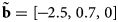 at locations: top elevation (χ = 0 km), mid-elevation (χ ≈ 2.5 km) and terminus elevation (χ ≈ 10 km). The green curve is the apparent mass-balance field corresponding to ${\tilde {\bf b}}$
 , which is the subtraction of the linear interpolation of ${\tilde {\bf b}}$
 from the expected value.

Brinkerhoff and others (Reference Brinkerhoff, Aschwanden and Truffer2016) approached the spatial variation of θ in a more sophisticated manner by sampling a Gaussian process to get a smooth realisation of a possible 1D field. This contrasts with our method, where the sampled 1D fields will not have any such smoothness (for instance, this is illustrated by the spikes of the green curve at x = 1 km and 10 km in Fig. 3). They also investigated the impact of the correlation length of their Gaussian processes. We did not conduct such a systematic analysis to determine the optimal number of components for each parameter (which implicitly sets the correlation length). Instead, simple trials paired with computational limitations (more parameters need more computational time) were used to select the numbers of components.
All the fitting parameters are given a prior distribution which is encoded as either a (i) uniform distribution given by a range, (ii) normal distribution given by a mean and standard deviation, or (iii) truncated normal distribution by combining the two (Table 2).
For f sl and T, there are essentially no measurements available and we limit their distribution to a plausible range. The fraction of basal sliding to surface speed must lie in the range 0 ≤ f sl ≤ 1 as sliding speed cannot be negative and cannot be larger than surface speed. Here, we assume a uniform distribution. We assume the ice temperature to have a truncated normal distribution with μ = −0.5°C, σ = 1°C and range −20°C < T < 0°C. This favours temperate glaciers, which we justify with the observation that the ice at depth of most larger glaciers (which contribute most of the volume, Farinotti and others, Reference Farinotti2019) will be at or close to the melting point. The thickness extrapolation parameter d is given a uniform prior in the range [0.1, 1], covering both U- and V-shaped valleys. The speed extrapolation parameter d v is a truncated normal distribution with μ = 4 (as Nye, Reference Nye1965 suggests), σ = 1/2 and range [0, 20].
As stated above, the expected value of the apparent mass balance is given by measurements, external models or guesses. For example, ∂h/∂t may be from remote sensing and $\dot {b}$ from a mass-balance model; these inputs will be discussed in Section 3. We can also put two constraints on the flux q, which is the integral of $\tilde b$
 (corresponding to a ${\tilde {\bf b}}$
 ) (Eqn (4)). First, we require that the glacier is continuous, which means that the flux is only allowed to go to zero at the top and at the computed terminus; in between we require q i > 0, otherwise the prior is set to zero. Second, for calving glaciers, the flux at the terminus q N will be non-zero. The distribution of q N(θ) is assumed normal with $\mu = 0.5 \dot {B}_{\rm acc}$
 and $\sigma = 0.1 \dot {B}_{\rm acc}$
 , where $\dot {B}_{\rm acc}$
 is the total accumulation. This is incorporated into the prior, assuming independence, by multiplying with the density p(q N(θ)) of this normal distribution. The chosen values of μ and σ are consistent with two estimates of calving flux that are available for two of the largest ice masses considered here (measurements or estimates of calving fluxes are not available on a global scale): Dowdeswell and others (Reference Dowdeswell, Benham, Strozzi and Hagen2008) state that for Austfonna ice cap, Svalbard, 44% of mass loss is through calving; similarly, Burgess and others (Reference Burgess, Sharp, Mair, Dowdeswell and Benham2005) state 40% for Devon Ice Cap, Arctic Canada.
We assume that all priors are independent of each other and, thus, the full prior p(θ) is the product of the individual ones.
2.2.3 Likelihood p(d|θ).
The forward model produces fields for the ice thickness h and surface speed v which need to be fitted to the measurements h′ and v′. In case of land-terminating glaciers, also the 1D glacier length l′ is fitted. This ensures that the 1D glacier reaches the end of the lowest elevation band but not further. The comparison between data and model is done with a simple stochastic model of the errors. As an approximation, it assumes that all errors are independent and have a normal distribution

where the forward model output h(θ) and the observations h′ are vectors of values at the coordinates (x′, y′) of the observation, whereas for v and v′ the vector components are at grid locations on the boundary of two elevation bands (see Section 2.1, step 4). For the comparison, the thickness result is interpolated to the measurement location (x′, y′) and vice versa for the speed. Note, if no observations are available for a variable, the corresponding term in Eqn (16) becomes one. The standard deviation of the error in h is $\sigma _{\rm h}=\sqrt {\sigma _{\rm h_m}^{2} + \sigma _{\rm h_o}^{2}}$ , combining the model-error standard deviation $\sigma _{\rm h_m}$
 and the observational-error standard deviation $\sigma _{\rm h_o}$
 ; the error of v and l are treated identically with a combined standard deviation σv and σl. The values of the observational-σ are a combination of the stated or estimated uncertainty of the data (see next section) and of the uncertainty stemming from non-simultaneous observations (Brinkerhoff and others, Reference Brinkerhoff, Aschwanden and Truffer2016). The model-σ is fitted (using a uniform prior with range [0, 200] m and [0, 200] m a−1 for σh and σv). The σ are assumed constant for all locations (x, y).
Equation (16) assumes independent errors. The errors of h and v, however, are spatially correlated, which is true for both the measurement and the model errors. To reduce this correlation, we adopted the simple strategy to thin out the points at which observations are compared to the model. For the thickness observations we achieved this by thinning the data such that the distance between observations is ~1/100th of the glacier length. For the ice speed, the model results are thinned instead, by a factor of ten in both coordinate directions resulting in a distance between comparison points of 250–2000 m (depending on DEM resolution).
Note that the calculation of the likelihood for a set of parameters θ involves the evaluation of the forward model using the θ-parameters to produce h(x, y, θ), v(x, y, θ) and l(θ). When fitting only to l′, just the 1D part of the forward model needs evaluating, which is ~200 times faster than evaluating the full 2D model.
With both the prior p(θ) and the likelihood p(d|θ) specified, the posterior can be evaluated (up to a normalisation factor, Eqn (13)).
2.2.4 Sampling from the posterior
We are interested in characterising the posterior p(θ|v′, h′), a high-dimensional probability distribution, which is best done using samples from it.
We use a MCMC method to draw the samples, a widely used approach for this type of analysis. We employ an affine-invariant ensemble sampler (Goodman and Weare, Reference Goodman and Weare2010; Foreman-Mackey and others, Reference Foreman-Mackey, Hogg, Lang and Goodman2013). MCMC methods require many model evaluations to draw enough samples to characterise the posterior. For our application, around 105 samples are necessary to obtain converged results. We analyse convergence using visual inspection of the MCMC traces as well as the potential scale reduction factor $\hat R$ (Gelman and others, Reference Gelman, Carlin, Stern and Rubin2014), which we calculate from MCMC chains from independent runs of the affine-invariant sampler (see Section S4 of the Supplementary Material).
An example inversion for Unteraar Glacier data is shown in Figure 4, with panel D displaying the distribution of samples from seven of the 11 θ components.
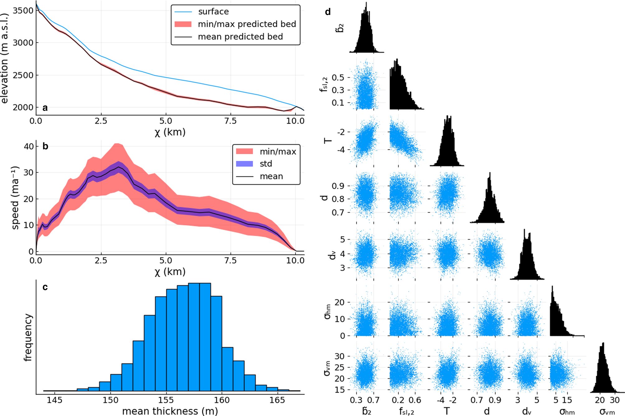
Inverse model output for test-case Unteraar from fitting the model to three radar lines (see Fig. 5f), glacier length and surface ice speed. (a) 1D glacier surface and predicted bed (mean, minimum and maximum); (b) predicted speed; (c) distribution of inferred mean ice thickness; and (d) distribution of a selection of fitting parameters. The diagonal shows the sample histograms for each, and the scatter plots the distribution between two variables.
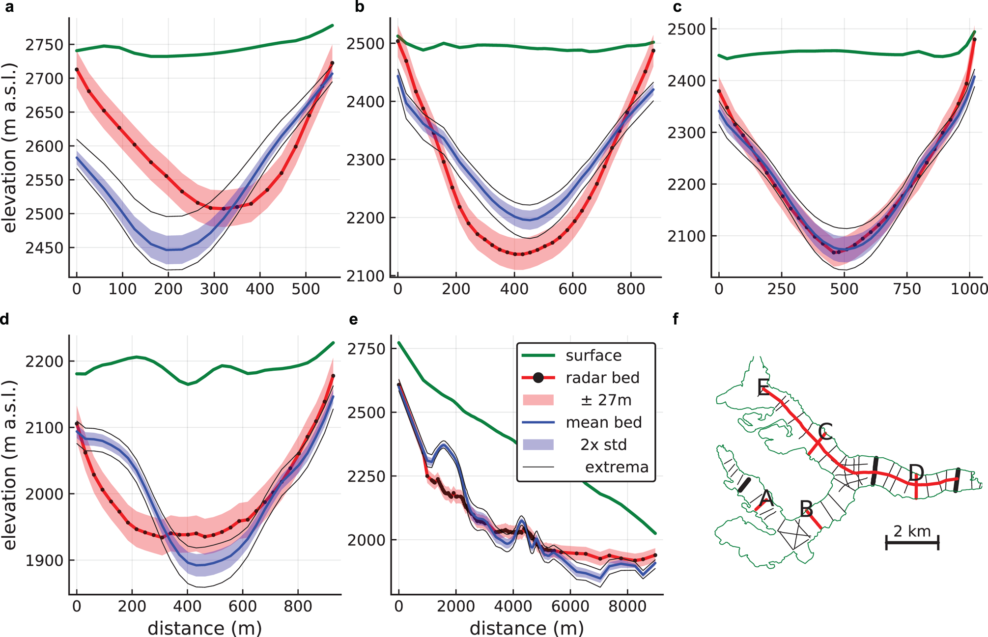
Comparison of ice thickness measurements based on ground-penetrating radar along profiles to inverted ice thickness for test-case Unteraar (a–e). (f) Glacier outline and radar tracks. The thick black lines are the fitting tracks, and the thick red lines are the ones displayed in a–e.
2.2.5 Predictions for h and v.
Whilst having the distribution of the parameters θ is useful, here we are primarily interested in the distribution of h and v, so-called predictions. During the MCMC procedure, the calculated h and v fields indeed represent samples from their posterior distributions and, thus, characterise them. This allows us to give both their expected values (the mean) as well as their distribution.
Predictions with associated uncertainty for the Unteraar test-case are displayed in Fig. 4. A comparison of the 2D predictions with thickness measurements along radar lines is displayed in Fig. 5.
2.3 Regional-scale applications
When applying our model to many glaciers, the typical situation will be that a few glaciers have ice thickness measurements but the vast majority do not. In that case, the few glaciers with thickness data can be fitted well whereas the others cannot be fitted, at least not to ice thickness. In this situation, we aim to transfer the knowledge gained from fitting the few glaciers to the majority of glaciers. We do so by using a representation of the posterior distributions obtained for glaciers with measurements as an update to the prior distribution for glaciers without measurements.
We first fit each glacier with thickness measurements individually (henceforth termed Mode-1) and thus obtain samples from their posterior distributions. We then translate these θ samples into a probability density function which can be used as part of a prior. We approximate this multidimensional density function by assuming that the parameters have independent normal distributions with (i) the central parameter given by the median (which we prefer over the mean to reduce the impact of outliers) of all Mode-1 expected values of θ, and (ii) the variance given by the variance of the combined posterior samples of all Mode-1 glaciers. The density function of this multivariate, uncorrelated normal distribution of θ is then multiplied with the density function of the usual prior (Section 2.2.2) to form the new prior for Mode-2 glaciers.
The new prior is then used for the rest of the glaciers, which are only fitted to their length (or only to the prior in case of calving glaciers), or to surface ice speed as well. Henceforth, we term this step Mode-2 fitting. The strategy is evaluated in the Results section.
2.4 Implementation
The BITE-model implementationFootnote 1, whose code is open source (see Section S2 of Supplementary Material), focuses on good computational performance as the MCMC scheme requires 104 to 105 forward model evaluations to fit one glacier. We use the Julia programming language (Bezanson and others, Reference Bezanson, Edelman, Karpinski and Shah2017), which achieves computational speeds on par with Fortran and C. As many calculations as possible are performed during glacier initialisation and then re-used during the MCMC computation; for instance the spatial smoothing, a linear operation, is pre-calculated and stored as a sparse matrix.
One forward model evaluation completes in ~0.01–0.1 s on a single core of a modern CPU (Intel Xeon E5-2687W), leading to Mode-1 fitting of one glacier completing in ~1 h. When not fitting to ice speed, Mode-2 runs complete in less than 1 min, as only the 1D part of the forward model needs to be evaluated to compute the glacier length. The regional fitting is an ‘embarrassingly parallel’ problem as different glaciers can be run at the same time and thus the work can trivially be distributed among several computers. The regional fitting for Svalbard, consisting of 170 Mode-1 and 1545 Mode-2 inversions (not fitting to ice speed), completes in ~10 h on a server with 12 physical cores (Intel Xeon E5-2687W, hyperthreaded), with ~80% of the time spent for the Mode-1 inversions.
As stated above, computational efficiency is one of the reasons to keep the DEM and outline constant. Changing them would necessitate the re-evaluation of most pre-processed computations, leading to an increase in forward model execution time – and thus Mode-1 fitting time – by a factor of ~50–200. Mode-2 runs would require an even higher increase in computational time.
The used affine invariant MCMC sampler is implemented in the package KissMCMC.jlFootnote 2. When generating the predictions of the 2D ice thickness and speed, not all samples can be retained due to their large memory footprint. Instead we only store the mean, standard deviation and extrema of the sampled h and v fields. We do this by using online statistical methods through the package OnlineStats.jlFootnote 3.
3. Study sites and data
Our study sites include Arctic Canada North (RGIv6.0 region 3) and South (region 4), Svalbard (region 7), Central Europe (region 11) and the Karakoram (region 14, subregion 2). The selected regions are depicted in Fig. 6 and contain about one-sixth (~30 000) of all glaciers worldwide by number and ~30% of the global glacier volume (Farinotti and others, Reference Farinotti2019). The selection of these regions was largely driven by data availability, i.e. measurements of ice thickness, elevation changes and/or surface ice speed. We consider this a globally-representative glacier sample suitable for demonstrating our model's applicability to large scales.
World map showing the considered RGI-regions, and examples ice thickness maps for each region: (3) Clarence Head N&S glaciers (76.74°N, 78.07°W); (4) Barnes Ice Cap (70.0°N, 73.5°W); (7) southern Spitsbergen around Vestre Torellbreen (77.3°N, 15.1°E); (11) Grosser Aletschgletscher (46.44°N, 8.08°E); (14) Biafo Glacier (75.59°N, 36.00°E).

3.1 Data
The necessary inputs for our forward model are summarised in Table 1. For all glaciers we use outlines from the RGIv6.0 (RGI-Consortium, 2017) and glacier mass balances from the Global Glacier Evolution Model (GloGEM) (Huss and Hock, Reference Huss and Hock2015). As DEMs we use the ArcticDEM (Porter and others, Reference Porter2018) and the SRTM (Space shuttle Radar Topography Mission) DEM (Jarvis and others, Reference Jarvis, Reuter, Nelson and Guevara2008). The elevation change datasets are more diverse and not available for all regions. The output of our model is ice thickness and surface speed (Table 1) which we compare to the Glacier Thickness Database (GlaThiDa) v3.0 (GlaThiDa-Cons, 2019) and a heterogeneous set of ice speed data. Note that most available datasets provide ice velocity, i.e. speed and azimuth, however our model only uses speed; therefore we use the word speed throughout except when the azimuth is important. Table 3 gives an overview over the used data.
Used data listed by RGI region and associated variable
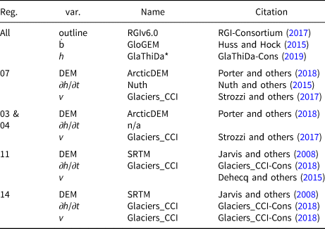
* No data available for region 14.
The RGIv6.0 dataset includes outlines of all glaciers worldwide as well as additional information on each glacier. The reference year for the outlines is included in the RGI attributes and more than 90% of the glaciers we consider lie in the time-span 1999–2010. We use the outline to delineate the glacier catchment in the map plane. It also determines the 1D glacier length for which we set an observational uncertainty $\sigma _{\rm l_o}$ of 3%; most of this uncertainty is due to non-simultaneous observations (Brinkerhoff and others, Reference Brinkerhoff, Aschwanden and Truffer2016). Furthermore, the outlines of adjacent glaciers determine the land mask which is used to calculate the distance-to-land L (Eqns (10) and (11)). From the additional RGI information, the attributes ‘Form’ and ‘TermType’ are used. ‘Form’ indicates whether the considered entity is a glacier or an ice cap (if un-assigned, we assume that it is a glacier), determining whether the 1D ice thickness at the top is set to zero or to the same as one elevation band below. ‘TermType’ distinguishes between land-terminating and calving glaciers, which determines whether the glacier length is fitted (Eqn (16)) or whether a terminus-flux prior is used. Note, however, that the classification is not very accurate, at least for Svalbard, and many calving glaciers are mis-labelled as land-terminating.
The ArcticDEM is a high-resolution (2 m) DEM of the Arctic using WorldView-1, 2 and 3 satellite data from the years 2007–2018. It is used for the regions Svalbard and Arctic Canada North and South. The SRTM DEM is available up to 60° North at a resolution of 30 m and was acquired in February 2000. It is used for the regions Central Europe and Karakoram. For each glacier the DEM is pre-processed by projecting it into the appropriate UTM zone, cropping it to fit the glacier outline, and re-sampling it to 25, 50, 100 or 200 m depending on the glacier size. The last step ensures that all DEMs have a similar resolution relative to the glacier size. The grid of the DEM is then also used as the computational and output grid for the forward model. Our model approach cannot take errors of DEMs into account (see Section 2.2). However, the study of Huss and Farinotti (Reference Huss and Farinotti2012) (using almost the same forward model) estimated the errors associated with using the SRTM for Central Europe and Karakoram to be ~1% of the regional ice volume and thus these errors are negligible compared to others.
The GloGEM computes past mass-balance components and their altitudinal distribution for all glaciers globally based on climate re-analysis data (see Huss and Hock, Reference Huss and Hock2015 for details). Results for each individual glacier have been calibrated to match the regional average mass balance between 2003 and 2009 (Gardner and others, Reference Gardner2013) and computed mass-balance gradients with elevation have been validated against a global dataset of direct observations (WGMS, 2012). Uncertainties for local mass-balance estimates are ~±1 m a −1. For each individual glacier, we use the average of GloGEM mass balances over the period 1980–2016.
The elevation change dataset for Svalbard is a difference between the Norwegian National DEM of 1990 and the SPOT5 DEM of 2008 (Nuth and others, Reference Nuth, Hagen and Kohler2015). The resolution is 40 m and the dataset covers most of the Spitsbergen south of Longyearbyen. For the rest of Svalbard we have no data. For the Karakoram, we use an elevation change dataset derived from differencing SRTM (from 2000) and TanDEM-X (from about 2013) DEMs with a posting of 90 m. Both DEMs have been horizontally and vertically co-registered before subtraction. As the radar penetration of the C and X band into snow and (dry) firn can be different and reach several metres, we have also analysed elevation differences over stable terrain. This revealed only small (a few metres) vertical and largely unsystematic differences. Given the large elevation changes over many glaciers (>100 m) and the vertical uncertainties of both DEMs (several metres), we consider differences in the radar penetration (i.e. not the individual absolute values) as negligible and have not further corrected them. For the Alps, elevation changes have been derived by differencing the SRTM C Band DEM from 2000 from the TanDEM-X DEM from about 2014, also with 90 m posting. Both datasets are provided by the ESA project Glaciers_CCI (Climate Change Initiative) (Glaciers_CCI-Cons, 2018). For all elevation change data we assume a normal error with standard deviation 1 m a−1 (e.g. Nuth and others, Reference Nuth, Moholdt, Kohler, Hagen and Kääb2010). We have no elevation change data for Arctic Canada North and South. For glaciers without elevation change data available, or when testing the impact of using elevation change data, we use a synthetic, elevation-dependent rate

where z ELA is the equilibrium line altitude provided by GloGEM, and c 1 and c 2 are constants adjusted such that the flux at the terminus is as specified. For glaciers where z ELA is above the top or below the terminus, a constant elevation-change rate is assumed. As an uncertainty we assume 2 m a−1.
We combine the uncertainty of the elevation-change data and GloGEM data assuming independence to get an uncertainty of the apparent mass balance on elevation bands. For the case of synthetic elevation change, this neglects that through the use of z ELA in Eqn (17) there will be some correlation of the errors. However, we expect this to be of minor importance and neglect it. The uncertainty is thus 1.4 m a−1 when elevation-change data are available and 2.2 m a−1 otherwise.
Ice thickness data, which are generally collected with ground penetrating radar, are available through GlaThiDa v3.0 (GlaThiDa-Cons, 2019) for 1084 of the 31 235 considered glaciers. However, we manually rejected 333 glaciers either due to all-zero thickness measurements within the area of the glacier outline or due to only marginal coverage of the glacier. The ratio between the number of glaciers with usable radar tracks and total for each region is: Svalbard 170/1615 (22 glaciers rejected), Arctic Canada North 315/4556 (150), Arctic Canada South 130/7416 (121), European Alps 136/3892 (30) and Karakoram 0/13757. The spatial density of observations is variable and dense observations are thinned such that the distance between them is ~1/100th of the glacier length (this thinning is also used to avoid spatial correlations in the likelihood, Section 2.2.3). Some data in GlaThiDa have an associated error, but we simply set the standard deviation to $\sigma _{\rm h_o}=10$ m.
m.
Surface ice speed for all regions but the Alps are from the Glaciers_CCI project. For Svalbard we use a dataset derived from feature tracking of Sentinel-1 images between January 2015 and January 2017 (Strozzi and others, Reference Strozzi, Paul, Wiesmann, Schellenberger and Kääb2017). For the Karakoram a dataset derived from Sentinel-1 SAR images acquired in 2015 using offset-tracking is used (Glaciers_CCI-Cons, 2018). The data for Arctic Canada North and South are derived from winter Sentinel-1 SAR images acquired in 2015 (Strozzi and others, Reference Strozzi, Paul, Wiesmann, Schellenberger and Kääb2017). For the European Alps, glacier surface speeds were generated by tracking surface features in Landsat 7 panchromatic images (15 m spatial resolution). Displacement fields were generated at 30 m resolution from all images separated by approximately one year over the period 1999–2003 and the median value for the whole period was retained in each pixel (Dehecq and others, Reference Dehecq, Gourmelen and Trouve2015, Reference Dehecq, Noel, Emmanuel, Jauvin and Rabatel2019b). This dataset is limited to the Western Alps including the area between Rhone Glacier and Mont Blanc. For the error of all ice speed data, we use a standard deviation $\sigma _{\rm v_o}=10$ m a−1 (e.g. Dehecq and others, Reference Dehecq, Gourmelen and Trouve2015). Note, however, that we fit $\sigma _{\rm v_m}$
 and $\sigma _{\rm h_m}$
 , which means that the values of $\sigma _{\rm v_o}$
 and $\sigma _{\rm h_o}$
 are not critical.
4. Results
We present the results of our model for three different setups: (i) we revisit the test glacier Unteraar, used in the Methods section, to illustrate various aspects of the model; (ii) we calibrate and validate the model using glaciers with ice thickness data from four RGI regions, with a focus on our method for regional-scale application; and (iii) we demonstrate the large-scale applicability of the BITE-model by applying it to 30 000 glaciers in five RGI regions. The results of the latter are compared to the G2TI initiative (Farinotti and others, Reference Farinotti2019).
4.1 Unteraar test case
The Unteraar Glacier test-case is taken from the ITMIX project (Farinotti and others, Reference Farinotti2017) which provides the following data: outline and surface DEM (year 2003), mass balance (1997–2003), elevation change (1997–2003), ice speed (1997, Vogel and others, Reference Vogel, Bauder and Schindler2012) and ice thickness along 45 radar tracks (Bauder and others, Reference Bauder, Funk and Gudmundsson2003) (Fig. 5f). All data but the outline and ice thickness measurements are provided on the same grid with a posting of 25 m, which is also the grid used for the model run. We use the priors as given in Table 2, with σ = 0.3 m a−1 for the apparent mass balance. For the ice thickness we assume an observational error of $\sigma _{\rm h_{o}}=27$ m (Bauder and others, Reference Bauder, Funk and Gudmundsson2003), for ice speed $\sigma _{\rm v_{o}}=4$
 m a−1 (Vogel and others, Reference Vogel, Bauder and Schindler2012) and for the glacier length $\sigma _{\rm l_o}=300$
 m (Unteraar Glacier retreated 400 m 1997–2004, GLAMOS, 2018). Of note is that Unteraar Glacier is debris-covered downstream of the confluence area.
For this test case, the model was fitted to the length of the glacier, the ice speed and to three radar tracks, one located in the upper accumulation area, one on the middle of the tongue and one close to the snout (Fig. 5f, thick black lines). Figure 2 shows the output of the forward model for the best fit parameters (i.e. the parameters with maximum posterior density), showing that visually the fit to observed ice thickness is very good (Fig. 2d). Ice speed in 2D is displayed at elevation-band boundaries which is where the error (Eqn (16)) is evaluated when fitting to ice speed.
The distributions of the fitting parameters are well approximated by the 105 samples taken (Fig. 4d). The distribution of ${\tilde {\bf b}}_2$ illustrates how the fitting procedure modifies its prior distribution with mean 0 m a−1 to a distribution with mean ~0.5 m a−1, i.e. the model needed to increase $\tilde {b}$
 around mid elevation to get a good fit. This can also be seen in Fig. 2c, where the fitted $\tilde {b}$
 is above the observed one at mid elevation (around χ = 2.5 km), whereas at the top and terminus the $\tilde {b}$
 was barely modified. The displayed parameters (Fig. 4d) are largely independent except for the negatively correlated fsl2 and T. This means that the inversion compensates slower flow due to stiffer ice with increased sliding.
The fitted model error for the ice thickness $\sigma _{\rm h_m}$ is 3 m, resulting in an effective σh ≈ 27 m. This is essentially unmodified from $\sigma _{\rm h_o}$
 . The mean ice thickness is ~157 m with a narrow spread of ±7 m (Fig. 4c) which is also reflected in the narrow band of predicted 1D bedrock elevations (Fig. 4a). Thus, the fitted σh amounts to 17% of mean ice thickness. For the ice speed, the effective σv is ~22 m a−1 (most of it due to model error as the observation has $\sigma _{\rm v_o}=4$
 m a−1) which is larger than the mean flow speed of ~16 m a−1 (Fig. 4b). This means that the model error is larger than the signal for many locations on the glacier. Thus, the model has very little predictive capability for surface speed, at least for this test case.
Figure 5 compares the thickness results against measurements along five radar tracks. The V-shaped valley profile along track C is matched best; indeed the d parameter, which controls the valley shape, is close to 1 thus indicating a V-shape. As d is constant for the whole glacier, track B, located in a U-shaped section of the glacier, is less well matched. At the two profiles A and D, the surface is sloping sideways or is undulating due to supraglacial debris coverage. This impacts the ice thickness extrapolation through the surface slope (Eqn (10)) in a partly unrealistic pattern. This could probably be alleviated by employing surface smoothing techniques that preferentially smooth across-flow rather than along-flow. However, the large mismatch of profile A at distance 0 m is likely caused by erroneous input data: the radar profile shows zero thickness whereas the outline is still further out. The longitudinal profile shows that the thickness is matched well except underestimating ice thickness at χ ≈ 2000 m and overestimating near the terminus. The latter is likely due to the strongly undulating surface there, as seen in profile D, located in this region.
Summarising, the BITE-model can predict the ice thickness of Unteraar Glacier well when fitted to three radar profiles, with the estimated ice thickness error at 17% of the mean ice thickness. However, the ice speed is not well matched, and its predicted errors are 137% of the mean speed.
4.2 Model validation against thickness measurements
We validate the BITE-model using test glaciers with available thickness measurements from RGI regions Arctic Canada North and South (regions 3 and 4), Svalbard (7) and Central Europe (11). The test focuses on (I) the relative importance of fitting individual variables for obtaining accurate glacier-scale ice thickness and (II) the performance of our proposed scheme for regional-scale applications (Section 2.3). To assess the latter we split the test glaciers of each region into a calibration and a validation set of equal cardinality and similar glacier-size distribution.
The model is fitted to each glacier in the calibration set in three different ways, using: (i) glacier length l, ice thickness h and ice speed v (labelled with lhv); (ii) length and speed (l-v); (iii) glacier length only (l--). In the Supplementary Material we also show the results of fitting to length and thickness (lh-) which are almost identical to the ones of lhv for all regions but Central Europe (11) where lh- estimates the thickness slightly better (see Supplementary Material, Figure S4). Note that lhv and lh- correspond to Mode-1 fitting, whereas l-- and l-v correspond to Mode-2 fitting without updated priors for the calibration glaciers. The errors of the ice thickness estimates of the calibration set are used to evaluate the relative importance of fitting to glacier length, ice speed and ice thickness.
Each glacier of the validation set we fit to length only (l--'), and length and speed (l-v'), using the priors updated from the calibration run lhv, as proposed in our scheme for regional model application (Section 2.3). This corresponds to Mode-2 fitting, with and without using ice speed measurements. This is used to assess the proposed scheme to transfer posterior knowledge to the priors of other glaciers for the two typically encountered cases of ‘no measurements available’ (apart from a glacier outline), and ‘ice speed measurements available from remote sensing’ (but no thickness measurements).
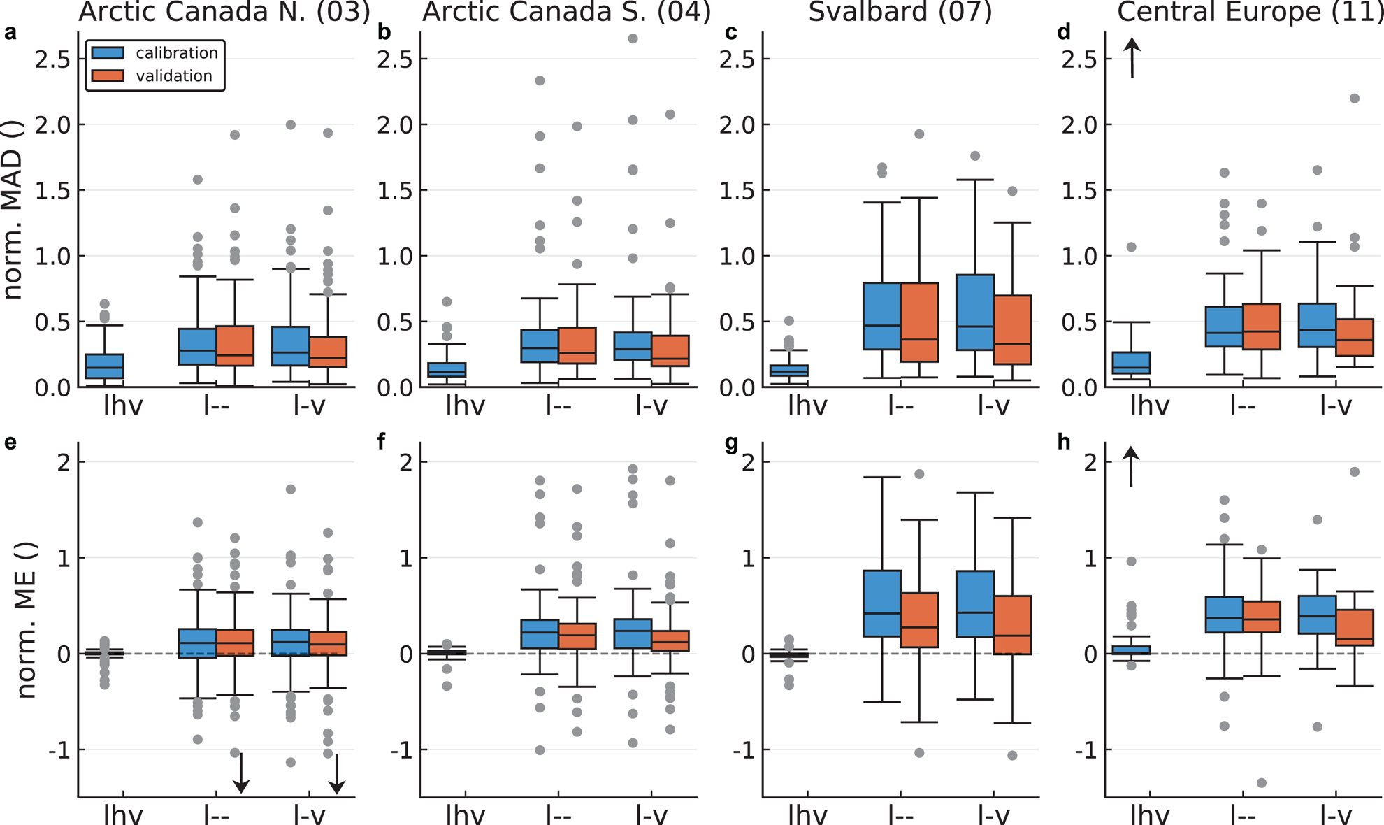
To evaluate the runs, we use the median absolute deviation (MAD), and the mean error (ME) of the ice thickness at the measurement locations, both normalised by the region-wide mean ice thickness (Section 4.3). The MAD gives an indication of how well the model can fit the basal topography, penalising both too shallow and too deep bed estimates. The ME will give an indication of the model's ability to estimate the total ice volume; in this case, too deep and too shallow local estimates can cancel each other out. We display the distribution of the normalised MADs and MEs of all test glaciers as box plots (Fig. 7). All the computed thickness maps are available for download (see Supplementary Material S3).
Distribution of ice thickness errors for various calibration (blue) and validation runs (red) for RGI regions 3 (panels a,e), 4 (b,f), 7 (c,g) and 11 (d,h). The first row shows the distribution of median absolute deviations normalised with mean regional ice thickness (norm. MAD), and the second row normalised mean errors (norm. ME). Positive ME values indicate that the model overestimates the ice thickness. The runs were fitted to the following observations: length l, ice thickness h and surface ice speed v (lhv); l only (l--); and l and v (l-v). The calibration runs used unmodified priors whereas the validation runs used priors updated with results from the lhv calibration run from the same region (see Section 2.3). Note that in the text the validation-run labels contain a prime (e.g. l--' vs. l--), however, the prime is not used in the plot-labels. The boxplots show the inter-quartile range (box), the median (horizontal line), the farthest data points within 1.5 times the inter-quartile range (whiskers), and individual outliers (dots). Arrows indicate that in D and H, one outlier at ~8 is not shown, and that in E, two outliers at ~−2 are not shown.
4.2.1 Relative importance of fit variables
For all regions, the median and the third quartile of the normalised MAD of the lhv calibration runs (Mode-1) are below 0.15 and 0.25, respectively (Figs 7a–d, blue boxes). This indicates that the model is well capable of fitting the observed ice thickness for Mode-1 runs. The calibration runs not fitted to thickness (l-- and l-v) show a much higher normalised MAD. For Arctic Canada most are still below 0.5 but for Svalbard and Central Europe the third quartile is above 0.5; the cause of the difference in MAD between the regions is not clear. Furthermore, the use of ice speed measurements does not improve the ice thickness estimations at all (cf. l-v vs. l--; an interpretation follows in the Discussion section).
The normalised ME shows a similar pattern (Figs 7e–h, blue boxes): Thelhv runs have a ME very close to zero (medians within ±0.015) with a very low spread (inter-quartile range ±0.07). Conversely, the l-- and l-v runs have a much larger spread, and show a model bias towards overestimated ice thickness in all regions. For Arctic Canada North and South, this bias is low (median ME ≈ 0.1) but for Svalbard and Central Europe it is large (median ME ≈ 0.5).
4.2.2 Evaluation of regional application scheme
The runs of the validation set, using the modified priors (Fig. 7, red boxes), show a slight improvement over the ones of the calibration set using the unmodified priors (corresponding blue boxes). However, the improvement is below 0.1 for the median of both MAD and ME, except for Svalbard where the improvement is more marked (up to 0.2) and, thus, the errors in Mode-2 glaciers remain about three times larger than for Mode-1 glaciers with a bias for ice thickness overestimation. Again, additionally fitting to ice speed measurements (l-v') does not improve ice thickness estimates versus fitting to length only (l--′), except slightly for Central Europe (Fig. 7h).
Summarising, only ice thickness observations seem to help in constraining our ice thickness estimates, whereas ice speed measurements do not show the anticipated benefit. Our scheme for regional model application – which aims at transferring posterior knowledge from Mode-1 fitting to Mode-2 fitting – seems to work in principle, albeit leading to modest improvements only.
4.3 Regional ice thickness and volume estimates
As a further test we apply our model to several RGI regions, and compare the results to the consensus estimates of three to five established ice thickness models (Huss and Farinotti, Reference Huss and Farinotti2012; Frey and others, Reference Frey2014; Fürst and others, Reference Fürst2017; Ramsankaran and others, Reference Ramsankaran, Pandit and Azam2018; Maussion and others, Reference Maussion2019) made in the frame of the recent G2TI study (Farinotti and others, Reference Farinotti2019).
In Mode-1, we fit the model to ice thickness measurements and glacier length (lh-). We update the priors of the Mode-2 fitting, for which we only fit glacier length (l--'), using the posteriors of the Mode-1 runs from the same region as described in Section 2.3. For the Karakoram, no ice thickness measurements are available and thus no Mode-1 runs are possible. In this case, the priors for the Mode-2 runs are instead constructed using the posteriors of the Mode-1 runs of the four other regions (fitted to available observed elevation-change data). All those Mode-1 runs are combined into one set and then used in the procedure described in Section 2.3.
The previous section showed that fitting to surface ice speed does not improve the thickness estimates, thus, we do not use ice speed in this section. Note that this omission, as a further benefit, also greatly reduces the total simulation time. We run two sets of simulations, one using observed and one using synthetic elevation-change data (Eqn (17)). This will allow to quantify the impact of using this type of data.
Figure 6 shows example maps of expected ice thickness for the considered regions (ice thickness maps for all roughly 30 000 evaluated glaciers, including error estimates, are made available; see Section S3 of Supplementary Material). A few glaciers show some elevation-band related artefacts, for example, the lobes in region 3. The model does not match ice thickness of separate glaciers connected at ice divides, and thus some step changes in thickness are visible, for instance at the divides of Barnes Ice Cap (region 4). Otherwise the produced maps look plausible.
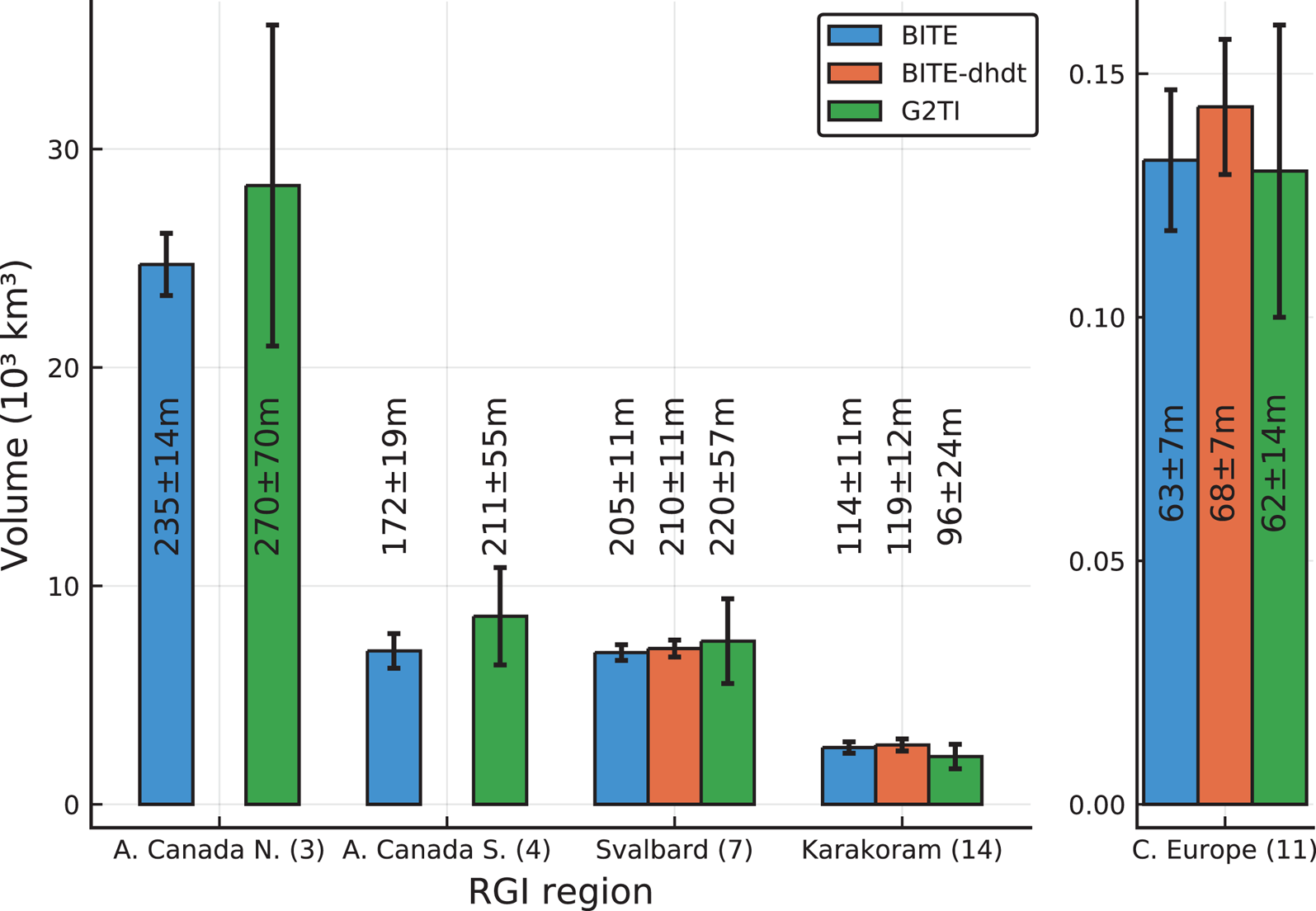
Figure 8 compares our estimates to the G2TI results. Using measured versus synthetic elevation-change data (Eqn (17)) has no significant impact on the results. All results fall within the error bounds of the G2TI results, with our error bars being considerably smaller than those of G2TI. We therefore suggest that our model's performance is comparable to that of other established global ice thickness models.
Total glacier ice volume (bars) and mean thickness (numbers) of the BITE-model in comparison to estimates of the G2TI study (Farinotti and others, Reference Farinotti2019) for the five considered RGI regions (note that RGI region 14 here only comprises subregion 2, i.e. the Karakoram). ‘BITE’ is our model using synthetic elevation-change data (Eqn (16)), ‘BITE-dhdt’ is our model using observed elevation-change data, and ‘G2TI’ is the consensus estimate from Farinotti and others (Reference Farinotti2019).
5. Discussion
One of the main motivations for this work was to make better use of surface ice speed measurements within the Huss and Farinotti (Reference Huss and Farinotti2012) model. The depth-averaged speed is constrained to lie within 80–100% of surface speed, according to the shallow ice approximation (Cuffey and Paterson, Reference Cuffey and Paterson2010). Thus, these measurements should be very valuable as they directly link to mass flux and ice thickness. Indeed, several other modelling approaches already make use of ice speed or velocity. However, unlike the presented model, these approaches either solve the mass-conservation equation (an advection equation, e.g. Morlighem and others, Reference Morlighem2011; McNabb and others, Reference McNabb2012; Brinkerhoff and others, Reference Brinkerhoff, Aschwanden and Truffer2016; Fürst and others, Reference Fürst2017), which critically depends on measurements of ice velocity, or use a full-scale ice dynamics model (e.g. Bueler and van Pelt, Reference Bueler and van Pelt2015), which is computationally expensive; and therefore these models are not as suited as our model for global-scale applications.
In contrast, our model skirts around those two issues by using a simple ice-flow model which algebraically relates ice thickness to flux and surface slope (Eqn (6)). Unfortunately, surface ice speed measurements do not improve our model results significantly. This is true in both the Unteraar test case (Fig. 4) and the model validation on four regions (Fig. 7). We speculate that this might be caused by a limitation of our forward model, or of the employed inversion procedure. One possible forward model limitation is that the ice speed approximately obeys v ∝ (1 − f sl) −1/(n+2) (combining Eqns (5), (6), (8)). This is a highly non-linear dependence with a singularity at f sl = 1 and implies that, for instance, f sl = 0.97 is needed to double the ice speed for a given flux. Combined with the uniform prior on f sl this could mean that parameters leading to higher speeds may have too low a probability to be selected. Thus, other sliding parameterisations should be explored in future work. Another possibility is that the shallow ice approximation formula (Eqn (6)) used in this study (and in many others) is not suitable for this type of application. Certainly, in steeper terrain (e.g. in Karakoram or Central Europe) its application is expected to lead to noticeable errors. Conversely, in flat terrain, such as dominating the large glaciers and ice caps of Arctic Canada (which make up most of those regions' ice volume), Eqn (6) should yield satisfactory results. However, our results for fitting ice speed (Fig. 7) are equally poor for all regions. A future study of the accuracy of Eqn (6) in ice thickness modelling applications is warranted, in particular as it is so widely employed. Last, our relatively simple likelihood function (Eqn (16)), assuming independence of all errors, could be the culprit. We do reduce spatial correlation of the errors by thinning out the points at which the likelihood is evaluated. However, a geostatistically more sophisticated error-model could make the likelihood more accurate and capable of appropriately weighting the ice speed and thickness errors and thus producing results consistent with both types of observations.
Despite our model's limitations regarding ice speed fitting, we note that the estimated regional total ice volumes are consistent with the G2TI consensus (Farinotti and others, Reference Farinotti2019). This is also the case for Svalbard, where the G2TI estimate is solely based on Fürst and others (Reference Fürst2018) who employed a model successfully using ice velocities (Fürst and others, Reference Fürst2017) (note also that the dataset of measured ice thicknesses available for Svalbard is very extensive). This finding is reminiscent of one of the conclusions of the ITMIX study (Farinotti and others, Reference Farinotti2017) which states: ‘Somewhat surprisingly, models that include SMB, ∂h/∂t, or surface flow velocity fields in addition to the glacier outline and DEM did not perform better when compared to approaches requiring less data, in particular for real-world cases’. The quote further highlights another of our findings, namely that the inclusion of elevation-change data does not significantly alter our regional results (Fig. 8), thus suggesting that accurate estimates of regional volumes also are possible with relatively scarce data input.
Bayesian inference has previously been applied to ice thickness estimation by Brinkerhoff and others (Reference Brinkerhoff, Aschwanden and Truffer2016). Their forward model is one of the above-mentioned models relying solely on the mass-conservation equation, which they originally applied to a 1D flow line, although within the framework of the ITMIX exercise it was applied in 2D (Farinotti and others, Reference Farinotti2017). Thus, their model is dependent on the availability of surface ice speed measurements whereas ours is reliant on the shallow-ice flow approximation being accurate enough. Our model's estimates of the thickness error are in general relatively small, both for single glaciers (e.g. Fig. 5) and at the regional scale (Fig. 8). Conversely, the model of Brinkerhoff and others (Reference Brinkerhoff, Aschwanden and Truffer2016) gives larger ice thickness uncertainties which nicely reduce where observations are available. This is due to their usage of Gaussian processes to sample bedrock elevations since they can incorporate observations more closely. In general, their approach uses more sophisticated statistical methods; for instance the usage of above-mentioned Gaussian processes to model the unknown fields whereas we just use a vector of parameters to modify given input fields (Fig. 3). However, their approach has not been demonstrated to be usable for large-scale applications – a main motivation for creating the BITE-model – which could in particular be hampered by its higher reliance on surface speed measurements; for instance in the ITMIX exercise the model was only applied to the synthetic cases ‘as velocity fields provided for the real cases had either insufficient spatial coverage or non-physical behaviour incompatible with the assumed model physics’ (supplement S1.1 of Farinotti and others, Reference Farinotti2017).
Our method is flexible, as it can utilise measurements where they are available and will fall back to prior assumptions in areas devoid of them. However, we also found that when measurements are of poor quality (which is often the case for small glaciers due to resolution issues, for instance) these measurements can adversely affect model performance. This is particularly true for Mode-2 runs, and care must thus be taken with the input data.
The model's flexibility makes it usable for large-scale applications to thousands of glaciers with heterogeneous data availability. Our basic setup uses the RGIv6.0 outlines, various DEM products and mass-balance model results (GloGEM), all available at the global scale. These data are enough to run the model and can be supplemented with ice thickness, elevation change and surface ice speed measurements where available. The application to five test RGI-regions shows that our model performs just as well as the ensemble of models in the G2TI-study (Farinotti and others, Reference Farinotti2019). So far, the predicted errors of our model are very small, and further investigation would be required to assess the reliability of these values.
The validation exercise showed that our method to transfer the knowledge gained from fitting glaciers with ice thickness measurements (Mode-1) to the priors used for glaciers without ice thickness measurements (Mode-2) works in principle. Yet, further refinements could benefit model performance. It is possible, for example, that other variables, for instance information about frontal-type (calving or land terminating), or surge-type, etc., would improve such a knowledge transfer. This could potentially also be achieved within a Bayesian framework. For instance, we could formalise our transfer model and make it dependent on variables such as frontal-type, and then fit this transfer model using Bayesian techniques. However, our previous observation also applies here: even though our transfer model might not be perfect, we match the region-wide estimates of established global thickness models. A possible reason is that the parameters of those models are not more effective than our transferred ones.
6. Conclusions
We presented the BITE-model which estimates glacier ice thickness distributions using a new inversion scheme based on Bayesian inference. The scheme is applied to an improved version of the forward model of Huss and Farinotti (Reference Huss and Farinotti2012). As input, the forward model needs a DEM, a glacier outline, an estimate of mass balance and elevation change. The outputs are an ice thickness map and a surface ice speed map. The latter two can then be fitted to observations during the inversion procedure. If there are no observations available, the Bayesian inversion can be run by using information gained from other glaciers.
The application of the model to individual glaciers, such as the presented test case of Unteraar Glacier, shows that the model performs well in such a setting, and that only a few radar profiles are needed for a reasonable fit. However, in a regional application where thickness measurements are only available for a few glaciers, our validation exercise shows that the average errors are larger. In such a case, the glaciers without thickness measurements are fitted using only prior information updated with the posteriors of the thickness-fitted glaciers, and this leads to an about threefold increase in thickness errors.
Our model is applicable on a large scale, which we demonstrate by applying it to five RGI regions with over 30 000 glaciers. This multi-regional application produces results consistent with the recent G2TI study (Farinotti and others, Reference Farinotti2019), suggesting that our model performance is comparable to that of an ensemble of existing models.
Our forward model is computationally very cheap, with one evaluation taking less than 0.1 s on a single core of a modern CPU. This allowed us to use Markov chain Monte Carlo methods for our Bayesian inference on a large number of glaciers. For the results included in this study, we calculated ~108 ice thickness maps and ~109 1D thickness fields. We think that this type of fast model, trading some accuracy for speed, has its place in large-scale applications where data availability and quality does not warrant to employ more computationally-intensive models. However, efforts are needed to extend this or similar frameworks to effectively assimilate surface flow speeds, which are becoming available at a fast rate. The other cornerstone of large-scale applications is consistent global datasets, such as RGI, GlaThiDa and various DEMs. Efforts are needed to extend and improve this kind of readily accessible and usable data.
Supplementary Material
The supplementary material for this article, which also contains the links/DOI-numbers to the model output data and code, can be found at https://doi.org/10.1017/jog.2019.93.
Acknowledgments
The work of MAW and FP was partly funded by the ESA project Glaciers_cci (4000109873/14/I-NB). We thank C. Nuth for providing the elevation-change dataset of Svalbard. Douglas Brinkerhoff, one anonymous reviewer and editor William Colgan provided valuable feedback which greatly improved the manuscript.


 Open access