


1. Introduction
Flexural waves are known to propagate through floating ice from classical experimental studies (e.g. Press et al. Reference Press, Crary, Oliver and Katz1951), and it is known from observations that the flexure can be forced by ocean waves (e.g. Holdsworth Reference Holdsworth1969). For over half a century, thin elastic plates (Lamb Reference Lamb1916) floating on water have been the benchmark model for ocean wave-induced flexural motions of sea ice (Evans & Davies Reference Evans and Davies1968; Wadhams et al. Reference Wadhams, Squire, Goodman, Cowan and Moore1988; Meylan & Squire Reference Meylan and Squire1994; Vaughan, Bennetts & Squire Reference Vaughan, Bennetts and Squire2009; Montiel, Squire & Bennetts Reference Montiel, Squire and Bennetts2016; Pitt et al. Reference Pitt, Bennetts, Meylan, Massom and Toffoli2022) and ice shelves (Holdsworth & Glynn Reference Holdsworth and Glynn1978; Vinogradov & Holdsworth Reference Vinogradov and Holdsworth1985; Fox & Squire Reference Fox and Squire1991b; Williams & Squire Reference Williams and Squire2007; Papathanasiou et al. Reference Papathanasiou, Karperaki, Theotokoglou and Belibassakis2015; Meylan et al. Reference Meylan, Ilyas, Lamichhane and Bennetts2021). The benchmark model, which dates back to Greenhill (Reference Greenhill1916), assumes the vertical ice displacements are uniform with respect to thickness (i.e. a thin plate), and the water is a potential-flow fluid. The plate appears in the model through flexural and inertial restoring forces at the water surface, which manifest as high-order derivatives in the dynamic surface condition. The high-order boundary condition supports so-called flexural-gravity waves, plus wave modes that have no analogue in open water (i.e. where the water surface is in contact with air), which are typically oscillatory decaying waves but can become purely decaying in certain regimes (Williams Reference Williams2006; Bennetts Reference Bennetts2007), as well as evanescent (exponentially decaying) modes.
In both sea ice and ice shelf applications, the canonical wave–ice interaction problem involves a two-dimensional water domain (one horizontal dimension plus depth), which has half of its surface covered by ice, and where motions are excited by an incident wave from the open (non-ice-covered) water (Evans & Davies Reference Evans and Davies1968; Tkacheva Reference Tkacheva2001; Linton & Chung Reference Linton and Chung2003). The incident wave is partially reflected at the ice edge and partially transmitted into the ice-covered domain. The model is used to predict, e.g. strains in landfast sea ice (Fox & Squire Reference Fox and Squire1991b, Reference Fox and Squire1994) and ice shelves (Fox & Squire Reference Fox and Squire1991a), and is the basis for models of wave attenuation in the marginal ice zone (Bennetts & Squire Reference Bennetts and Squire2012a,Reference Bennetts and Squireb). Although the Archimedean draught of ice is  ${\approx }90$ % of its thickness, the thinness of sea ice has been used to justify the so-called shallow-draught approximation, in which the ice floats at the water surface with no submergence. Therefore, the ice edge experiences no loading, and free edge conditions are applied (i.e. zero bending moment and shear stress). The water and ice are coupled along the underside of the ice only.
Methods have been developed to accommodate Archimedean ice draught, whilst retaining the free edge conditions (Williams & Porter Reference Williams and Porter2009; Montiel, Bennetts & Squire Reference Montiel, Bennetts and Squire2012; Papathanasiou, Karperaki & Belibassakis Reference Papathanasiou, Karperaki and Belibassakis2019). The methods address the geometrical corner created by the partial submergence of the ice edge, but not the additional water–ice coupling created by the bending moment applied by the water motion on the ice edge and the kinematic coupling between the ice edge and the water (equality of the normal water and ice displacements at their interface). Notably, Porter & Porter (Reference Porter and Porter2004), and subsequently Bennetts, Biggs & Porter (Reference Bennetts, Biggs and Porter2007), derived the free edge conditions as the natural conditions of a variational principle, but where the thinness of the plate was already applied in the underlying Lagrangian, i.e. a one dimensional body was partially submerged in a two-dimensional fluid.
Although ad hoc, the use of the shallow-draught approximation and/or free edge conditions at a sea ice edge seems unlikely to have a major impact on model predictions, as the ice thickness (typically tens of centimetres to a few metres) is much smaller than other characteristic lengths. Relevant wavelengths are in the swell regime (tens to hundreds of metres; wave periods 10–30 s) and wave–sea ice interactions typically occur in the deep ocean ( ${>}1$ km, i.e. much greater than wavelengths). In contrast, ice shelves are hundreds of metres thick, occur on continental shelves and the sub-ice shelf water cavities are typically hundreds of metres deep. Ice shelves vibrate in response to ocean waves from long swell (wavelengths on the order of hundreds of metres) to infragravity waves (wavelengths on the order of kilometres to tens of kilometres; wave periods 50–300 s) and longer (Chen et al. Reference Chen, Bromirski, Gerstoft, Stephen, Lee, Yun, Olinger, Aster, Wiens and Nyblade2019). Therefore, the jump in water depth created by the ice draught affects model predictions (Kalyanaraman et al. Reference Kalyanaraman, Bennetts, Lamichhane and Meylan2019).
For the ice shelf application, water–ice coupling at the submerged portion of the shelf front (i.e. the ice edge) appears likely to influence model predictions for incident swell. There is compelling evidence that swell forced shelf front strains strong enough to trigger runaway ice shelf disintegrations, which makes this missing aspect of the benchmark thin-plate model conspicuous (Massom et al. Reference Massom, Scambos, Bennetts, Reid, Squire and Stammerjohn2018). Abrahams et al. (Reference Abrahams, Mierzejewski, Dunham and Bromirski2023) recently analysed a numerical time domain simulation, in which the ice shelf is modelled using the full (linear) equations of elasticity. In addition to flexural waves, they identified extensional waves in the shelf that are generated by water–ice coupling at the shelf front. There is also observational evidence of ocean waves forcing extensional waves in ice shelves (Chen et al. Reference Chen, Bromirski, Gerstoft, Stephen, Wiens, Aster and Nyblade2018). (See Hunkins (Reference Hunkins1960), for observations of extensional waves in sea ice.) Further, Abrahams et al. (Reference Abrahams, Mierzejewski, Dunham and Bromirski2023) showed that extensional wave displacement amplitudes exceed those of the flexural waves for low frequencies, with the extensional to flexural amplitude ratio tending to infinity as the frequency tends to zero. Kalyanaraman et al. (Reference Kalyanaraman, Meylan, Bennetts and Lamichhane2020) analysed numerical computations in the frequency domain of an ice shelf (of finite length) modelled using the full equations of elasticity (although neglecting gravity), but applied free edge conditions at the shelf front. They found that the flexural displacement profiles were similar to those predicted by the benchmark model, at least for two wave periods in the infragravity regime. The finding is broadly consistent with the results of studies using the shallow-draught approximation and thick-plate models (Fox & Squire Reference Fox and Squire1991a; Balmforth & Craster Reference Balmforth and Craster1999).
In this article, we outline a variational principle that derives the governing equations of the ice shelf problem, where the shelf has an Archimedean draught and is modelled by the full equations of elasticity, i.e. no simplifying assumptions are made about the ice displacements. We use the variational principle to derive a thin-plate approximation by constraining the ice displacements to low-order subspaces, with the underlying assumption that the ice thickness is small with respect to the wavelengths it supports. The thin-plate approximation extends the benchmark model by including extensional waves in the shelf and coupling water and ice motions at the shelf front. We combine the thin-plate approximation with a single-mode approximation in the water, which involves averaging with respect to depth, similar to Porter & Porter (Reference Porter and Porter2004) and Bennetts et al. (Reference Bennetts, Biggs and Porter2007). We use the approximations to investigate the influence of coupling at the ice edge and extensional waves on ice shelf strains, across the swell and infragravity wave regimes.
2. Preliminaries
Consider a two-dimensional domain of homogeneous, inviscid and irrotational water, which has an (undisturbed) finite depth  $H$ and infinite horizontal extent (figure 1). An ice shelf of finite thickness $h$ and semi-infinite length covers the surface of the right-hand side of the water domain. Let the Cartesian coordinate system $(x,z)\equiv (x_{1},x_{2})$ define locations in the water and ice shelf. The horizontal coordinate, $x\in \mathbb {R}$, has its origin set to coincide with the shelf front. The vertical coordinate, $z$, has its origin set to coincide with the undisturbed water surface, such that the (flat) bed is located at $z=-H$.
Schematic (not to scale) of the equilibrium geometry.

The ice shelf is assumed to be a homogenous, isotropic, purely elastic solid without gravitational pre-stress (see Appendix A for simplified calculations suggesting the gravitational pre-stress has little effect on wave propagation). It has an Archimedean draught, such that its (undisturbed) lower surface is located at
 \begin{equation} z=-d\equiv-\frac{\rho_{{i}} h}{\rho_{{w}}}, \end{equation}
where  $\rho _{{i}}=922.5\ {\rm kg}\ {\rm m}$ $^{-3}$ and $\rho _{{w}}=1025\ {\rm kg}\ {\rm m}$ $^{-3}$ are the ice and water densities, respectively, such that $\rho _{{i}} / \rho _{{w}}=0.9$. The ice/water domain is partitioned into the ice shelf, the sub-shelf water cavity and the open ocean (figure 1), respectively,
 $$\begin{align} \varOmega_{{sh}} &= \{(x,z): 0< x<\infty; -d< z< h-d\}, \end{align}$$
 $$\begin{align}\varOmega_{{ca}} &= \{(x,z): 0< x<\infty; -H< z<-d\}, \end{align}$$
 $$\begin{align}\text{and}\quad \varOmega_{{op}} &= \{(x,z): -\infty< x<0; -H< z<0\}. \end{align}$$
The sub-domains (2.2) are assumed to be the equilibrium state of the ice/water system, about which motions are forced by incident waves.
Small amplitude (linear) motions of the ice–water system are considered. Let the displacement field be
 \begin{equation} \boldsymbol{u}(x,z,t)=[U(x,z,t);W(x,z,t)]\equiv[U_{1}(x,z,t);U_{2}(x,z,t)]. \end{equation}
The displacement in the  $y$-direction (or $x_{3}$-direction; which points out of the page in figure 1) is $V$ or $U_3\equiv 0$. In the ice, the infinitesimal strain tensor, $\boldsymbol {\varepsilon }(x,z,t),$ is defined as
 \begin{equation} \varepsilon_{ij} \equiv \tfrac{1}{2}(U_{j,x_{i}} + U_{i,x_{j}})\quad\text{for }{i,j \in \{1,2,3\}}. \end{equation}
The Cauchy stress tensor,  $\boldsymbol {\sigma }(x,z,t)$ (i.e. the stress tensor under infinitesimal deformation), is related to the strain tensor via the standard constitutive relations, such that
 \begin{equation} \varepsilon_{ij} =-\frac{\nu}{E} \delta_{ij}\sum_{r=1}^{3}\sigma_{rr} + \frac{1+\nu}{E} \sigma_{ij} \quad\text{for } i,j\in\{1,2,3\} , \end{equation}
where  $E$ is Young's modulus and $\nu$ is Poisson's ratio, and $E=11$ GPa and $\nu =0.3$ are used as standard values for ice shelves. Plane strain is assumed in the $x$–
$x$– $z$ plane, i.e. $\varepsilon _{3i} = \varepsilon _{i3} = 0$ (for $i=1,2,3$) but $\sigma _{33}$ is non-zero.
In the water, which is modelled as inviscid, the stress tensor has components
 \begin{equation} \sigma_{ij}=-P \delta_{ij} \quad\text{for } i,j\in\{1,2,3\}, \end{equation}
where  $P(x,z,t)$ is the pressure field. Assuming the water undergoes irrotational motions in the $x$–
$x$– $z$ plane (with no motion in the $y$-direction), the displacement field is expressed as the gradient of a scalar displacement potential, $\varPhi (x,z,t)$. At this stage, no relation is assumed between the pressure and the displacement potential, i.e. the Bernoulli equation is not applied. The functions $\zeta _{\bullet }(x,t)$ denote the vertical displacements of the water–atmosphere, water–ice and ice–atmosphere interfaces ( $\bullet =w\text {--}a,w\text {--}i,i\text {--}a$, respectively). They are not yet related to the ice displacements ( $\boldsymbol {u}$), water pressure ( $P$) or displacements (through $\varPhi$).
The relative hydrostatic pressures in the open ocean, ice shelf and sub-shelf water cavity are, respectively,
 \begin{align} P_{{op}}(z) =- \rho_{{w}} g z, \quad P_{{sh}}(z) = P_{0} - \rho_{{i}} g (z+d) \quad \text{and}\quad P_{{ca}}(z) = P_{0} - \rho_{{w}} g (z+d) =-\rho_{{w}} g z, \end{align}
where
 \begin{equation} P_0=P_{{sh}}(-d)=P_{{ca}}(-d)=P_{{op}}(-d)= \rho_{{i}} g h=\rho_{{w}} g d, \end{equation}
and  $g=9.81\ {\rm m}\ {\rm s}$ $^{-2}$ is the constant of gravitational acceleration. Note that $P_{{sh}}(h-d)=P_{{op}}(0)=0$, so (2.7a–c) represents the true hydrostatic pressure minus the constant atmospheric pressure, $P_{{at}}$, and that the hydrostatic pressure is continuous going from the open ocean into the sub-shelf cavity.
3. Variational principle
3.1. Lagrangian
The Lagrangian for the ice–water system is
 \begin{align} \mathcal{L}\{\boldsymbol{u},\varPhi,P,\boldsymbol{\zeta},\boldsymbol{\tau}\} =\mathcal{L}_{{sh}}\{\boldsymbol{u},\zeta_{i-a},\zeta_{w-i}, \boldsymbol{\tau}\}+ \mathcal{L}_{{ca}}\{\varPhi,P,\zeta_{w-i},\boldsymbol{\tau}\} +\mathcal{L}_{{op}}\{\varPhi,P,\zeta_{w-a},\boldsymbol{\tau}\}, \end{align}
where  $\mathcal {L}_{{sh}}$, $\mathcal {L}_{{ca}}$ and $\mathcal {L}_{{op}}$ are the Lagrangians for the ice shelf, sub-shelf water cavity and open ocean, respectively.
The (linearised) Lagrangian for the ice shelf is expressed as  $\mathcal {L}_{{sh}}=\mathcal {T}_{{sh}}-\mathcal {V}_{{sh}}$, where $\mathcal {T}_{{sh}}$ and $\mathcal {V}_{{sh}}$ are the kinetic and potential energies in the ice shelf, respectively. The kinetic energy is
 \begin{equation} \mathcal{T}_{{sh}} \{\boldsymbol{u}\} =\frac{\rho_{{i}}}{2} \iint_{\varOmega_{{sh}}} \{ U_{t}^{2} + W_{t}^{2}\} \,\mathrm{d}\kern0.06em x\,\mathrm{d} {z}. \end{equation}
The potential energy is the integral of the strain energy density plus the gravitational potential over the shelf domain, plus integrals from linearisation of the moving boundaries and normal stresses applied to the boundaries (denoted  $\tau _{ii}$; applied shear stresses, $\tau _{ij}$ for $i\neq j$, are neglected as the surrounding water and air do not support them). The strain energy density is
 \begin{equation} v_{{e}}(\boldsymbol{\varepsilon}) = \frac{1}{2} \sum_{i=1}^{2}\sum_{j=1}^{2}\sigma_{ij} \varepsilon_{ij}, \end{equation}
which depends only on the strain since (2.5) can be inverted to write the stress in terms of the strain.
The gravitational potential is calculated relative to the upper surface of the shelf ( $z=h-d$), as
 \begin{equation} P_{{sh}}(z-W) = \rho_{{i}} g (W-z+h-d). \end{equation}
Therefore, the potential energy in the ice shelf is
 \begin{align} \mathcal{V}_{{sh}}
\{\boldsymbol{u},\zeta_{i-a},\zeta_{w-i},\boldsymbol{\tau}\} & = \iint_{\varOmega_{{sh}}} \left( \frac{1}{2}
\sum_{i=1}^{2}\sum_{j=1}^{2}\sigma_{ij} \varepsilon_{ij} +
\rho_{{i}} g (W-z+h-d) \right) \,\mathrm{d}\kern0.06em
x\,\mathrm{d} {z}\nonumber\\ & \quad + \int_{0}^{\infty}
\left[\rho_{{i}} g W\,\zeta_{i-a} -\frac12
\rho_{{i}} g \zeta_{i-a}^2 -\tau_{22} W
\right]_{z=h-d}\,\mathrm{d}\kern0.06em x \nonumber\\ &
\quad -\int_{0}^{\infty} \left[(P_{0}+\rho_{{i}} g
W)\,\zeta_{w-i} -\frac12 \rho_{{i}} g
\zeta_{w-i}^2 -\tau_{22} W \right]_{z=-d}
\,\mathrm{d}\kern0.06em x\nonumber\\ & \quad
-\int_{-d}^{h-d} \left[ \tau_{11} U \right]_{x=0}^{\infty}
\,\mathrm{d} z.
\end{align}
\begin{align} \mathcal{V}_{{sh}}
\{\boldsymbol{u},\zeta_{i-a},\zeta_{w-i},\boldsymbol{\tau}\} & = \iint_{\varOmega_{{sh}}} \left( \frac{1}{2}
\sum_{i=1}^{2}\sum_{j=1}^{2}\sigma_{ij} \varepsilon_{ij} +
\rho_{{i}} g (W-z+h-d) \right) \,\mathrm{d}\kern0.06em
x\,\mathrm{d} {z}\nonumber\\ & \quad + \int_{0}^{\infty}
\left[\rho_{{i}} g W\,\zeta_{i-a} -\frac12
\rho_{{i}} g \zeta_{i-a}^2 -\tau_{22} W
\right]_{z=h-d}\,\mathrm{d}\kern0.06em x \nonumber\\ &
\quad -\int_{0}^{\infty} \left[(P_{0}+\rho_{{i}} g
W)\,\zeta_{w-i} -\frac12 \rho_{{i}} g
\zeta_{w-i}^2 -\tau_{22} W \right]_{z=-d}
\,\mathrm{d}\kern0.06em x\nonumber\\ & \quad
-\int_{-d}^{h-d} \left[ \tau_{11} U \right]_{x=0}^{\infty}
\,\mathrm{d} z.
\end{align}
The atmospheric pressure,  $P_{{at}}$, appears implicitly in (3.5) via the applied stresses
 \begin{equation} [\tau_{11}]_{x=0,0< z< h-d} =[\tau_{22}]_{x>0,z=h-d} \equiv-P_{{at}}. \end{equation}
 The Lagrangian for the sub-shelf water cavity is expressed as  $\mathcal {L}_{{ca}}=\mathcal {T}_{{ca}}-\mathcal {V}_{{ca}}$, where the kinetic energy in the water cavity is
 \begin{equation} \mathcal{T}_{{ca}} \{\varPhi\} = \frac{\rho_{{w}}}{2} \iint_{\varOmega_{{ca}}} \{ \varPhi_{xt}^{2} + \varPhi_{zt}^{2}\} \,\mathrm{d}\kern0.06em x\,\mathrm{d} {z} . \end{equation}
For the potential energy, a term that is analogous to the strain energy density in the ice is
 \begin{equation} v_{{e}}(P,\varPhi)=-P \nabla^{2}\varPhi, \end{equation}
and the gravitational potential is relative to the water surface (without the ice shelf;  $z=0$), i.e.
 \begin{equation} P_{{ca}}(z-\varPhi_{z}) = \rho_{{i}} g (\varPhi_{z}-z). \end{equation}
Therefore, the potential energy is
 \begin{align} \mathcal{V}_{{ca}} \{\varPhi,P,\zeta_{w-i},\boldsymbol{\tau}\} & = \iint_{\varOmega_{{ca}}} \{-P \nabla^{2}\varPhi + \rho_{{i}} g (\varPhi_{z}-z) \} \,\mathrm{d}\kern0.06em x\,\mathrm{d} {z}\nonumber\\ & \quad +\int_{0}^{\infty} \left[(P_0 + \rho_{{w}} g \varPhi_z)\,\zeta_{w-i} -\frac12 \rho_{{w}} g \zeta_{w-i}^2 -\tau_{22} \varPhi_z \right]_{z=-d} \,\mathrm{d}\kern0.06em x\nonumber\\ & \quad-\int_{0}^{\infty} [-\tau_{22} \varPhi_z ]_{z=-H} \,\mathrm{d}\kern0.06em x\nonumber\\ & \quad - \int_{-H}^{-d} [\tau_{11} \varPhi_x ]_{x=0}^{\infty} \,\mathrm{d} z . \end{align}
 Similarly, the linearised Lagrangian for the open ocean is  $\mathcal {L}_{{op}}=\mathcal {T}_{{op}}-\mathcal {V}_{{op}}$, in which
 \begin{equation} \mathcal{T}_{{op}} \{\varPhi\} =\frac{\rho_{{w}}}{2} \iint_{\varOmega_{{op}}} \{ \varPhi_{xt}^{2} + \varPhi_{zt}^{2}\} \,\mathrm{d}\kern0.06em x\,\mathrm{d} {z}, \end{equation}
and
 \begin{align} \mathcal{V}_{{op}} \{\varPhi,P,\zeta_{w-a},\boldsymbol{\tau}\} & = \iint_{\varOmega_{{op}}} \{-P \nabla^{2}\varPhi + \rho_{{i}} g (\varPhi_{z}-z) \} \,\mathrm{d}\kern0.06em x\,\mathrm{d} {z}\nonumber\\ & \quad + \int_{-\infty}^{0} \left[\rho_{{w}} g \varPhi_z\,\zeta_{w-a} - \frac12 \rho_{{w}} g \zeta_{w-a}^2 - \tau_{22} \varPhi_z \right]_{z=0} \,\mathrm{d}\kern0.06em x \nonumber\\ & \quad - \int_{-\infty}^{0} [ -\tau_{22} \varPhi_z ]_{z=-H} \,\mathrm{d}\kern0.06em x \nonumber\\ & \quad + \int_{-H}^{0} [ -\tau_{11} \varPhi_x ]_{x\to-\infty}^{0} \,\mathrm{d} z . \end{align}
Again, the atmospheric pressure appears implicitly, via
 \begin{equation} [\tau_{22}]_{x<0,z=0}\equiv-P_{{at}}. \end{equation}
Small variations are applied to all unknowns, such that the Lagrangians become
 \begin{equation} \mathcal{T}_{{sh}}\{\boldsymbol{u}+\delta\boldsymbol{u}\} =\mathcal{T}_{{sh}}\{\boldsymbol{u}\} +\delta \mathcal{T}_{{sh}}\{\boldsymbol{u}:\delta{}\boldsymbol{u}\} +{o}(\delta{}\boldsymbol{u}), \quad\text{and so on.} \end{equation}
The first variation of the full Lagrangian,  $\delta \mathcal {L}\{\boldsymbol {u},\varPhi,P,\boldsymbol {\zeta }, \boldsymbol {\tau }:\delta \boldsymbol {u},\delta \varPhi,\delta {}P, \delta \boldsymbol {\zeta },\delta \boldsymbol {\tau }\}$, is
 \begin{equation} \delta\mathcal{L} = \delta\mathcal{L}_{{sh}}+\delta\mathcal{L}_{{ca}}+\delta\mathcal{L}_{{op}} =\delta\mathcal{T}_{{sh}}-\delta\mathcal{V}_{{sh}} +\delta\mathcal{T}_{{ca}}-\delta\mathcal{V}_{{ca}} +\delta\mathcal{T}_{{op}} -\delta\mathcal{V}_{{op}}. \end{equation}
3.2. Action
The action,  $\mathcal {A}$, is the integral of the Lagrangian over an arbitrary time interval, $t_{0}< t< t_{1}$, i.e.
 \begin{equation} \mathcal{A}\{\boldsymbol{u},\varPhi,P,\boldsymbol{\zeta},\boldsymbol{\tau}\} =\int_{t_{0}}^{t_{1}} \mathcal{L}\{\boldsymbol{u},\varPhi,P,\boldsymbol{\zeta},\boldsymbol{\tau}\} \,\mathrm{d} t. \end{equation}
Its first variation is
 \begin{align} \delta\mathcal{A}\{\boldsymbol{u},\varPhi,P,\boldsymbol{\zeta}, \boldsymbol{\tau}:\delta\boldsymbol{u},\delta\varPhi,\delta{}P, \delta\boldsymbol{\zeta},\delta\boldsymbol{\tau}\} = \int_{t_{0}}^{t_{1}} \delta\mathcal{L}\{\boldsymbol{u},\varPhi,P,\boldsymbol{\zeta}, \boldsymbol{\tau}:\delta\boldsymbol{u},\delta\varPhi,\delta{}P, \delta\boldsymbol{\zeta},\delta\boldsymbol{\tau}\} \,\mathrm{d} t. \end{align}
From (3.1)–(3.15), the first variation is evaluated as
 \begin{align} \delta\mathcal{A} &
=-\int_{t_{0}}^{t_{1}} \iint_{\varOmega_{{sh}}} \{
\delta{}U (\rho_{{i}} U_{tt} - \sigma_{11,x} -
\sigma_{12,z})\nonumber\\ & \quad + \delta{}W (\rho_{{i}}
W_{tt} - \sigma_{21,x} - \sigma_{22,z} + \rho_{{i}} g) \}
\,\mathrm{d}\kern0.06em x\,\mathrm{d} {z}\,\mathrm{d}
t\nonumber\\ &\quad+ \int_{t_{0}}^{t_{1}}
\iint_{\varOmega_{{ca}}} \{ \delta{}P \nabla^{2}\varPhi +
\delta{}\varPhi \nabla^{2}\hat{P} \}
\,\mathrm{d}\kern0.06em x\,\mathrm{d} {z}\,\mathrm{d}
t\nonumber\\ & \quad + \int_{t_{0}}^{t_{1}}
\iint_{\varOmega_{{op}}} \{ \delta{}P \nabla^{2}\varPhi +
\delta{}\varPhi \nabla^{2}\hat{P} \}
\,\mathrm{d}\kern0.06em x\,\mathrm{d} {z}\,\mathrm{d}
t\nonumber\\ & \quad - \int_{t_{0}}^{t_{1}}
\int_{0}^{\infty} [ \delta\zeta_{i-a}
\rho_{{i}} g (W-\zeta_{i-a})\nonumber\\ &\quad + \delta{}W (\sigma_{22}+\rho_{{i}}
g \zeta_{i-a} +P_{{at}}) +\delta{}U
\sigma_{12} ]_{z=h-d} \,\mathrm{d}\kern0.06em x
\,\mathrm{d} t\nonumber\\ & \quad + \int_{t_{0}}^{t_{1}}
\int_{0}^{h-d} [ \delta{}W \sigma_{12} + \delta{}U
(\sigma_{11}+P_{{at}}) ]_{x=0} \,\mathrm{d} z \,\mathrm{d}
t\nonumber\\ & \quad + \int_{t_{0}}^{t_{1}}
\int_{0}^{\infty} [\delta\zeta_{w-i}
\{\rho_{{i}} g (W-\zeta_{w-i})- \rho_{{w}} g
(\varPhi_{z}-\zeta_{w-i})\}\nonumber\\
&\quad + \delta{}W (\sigma_{22}+\rho_{{i}}
g \zeta_{w-i}-S_{{bt}}) + \delta{}U
\sigma_{12}\nonumber\\ & \quad -
\delta\varPhi \hat{P}_{z} +\delta\varPhi_{z} (P-\rho_{{w}}
g \zeta_{w-i}+S_{{bt}}) -\delta{}S_{{bt}}
(W-\varPhi_{z}) ]_{z=-d} \,\mathrm{d}\kern0.06em x
\,\mathrm{d} t\nonumber\\ & \quad + \int_{t_{0}}^{t_{1}}
\int_{-d}^{0} [\delta{}W \sigma_{12} +\delta{}U
(\sigma_{11}-S_{{fr}}) -\delta\varPhi
\hat{P}_{x}\nonumber\\ & \quad +
\delta\varPhi_{x} (P+S_{{fr}}) -\delta{}S_{{fr}}
(U-\varPhi_{x}) ]_{x=0}\,\mathrm{d} z \,\mathrm{d}
t\nonumber\\ & \quad + \int_{t_{0}}^{t_{1}}
\int_{-\infty}^{\infty} [\delta\varPhi \hat{P}_{z}
-\delta\varPhi_{z} (P+S_{{bd}}) -\delta{}S_{{bd}}
\varPhi_{z} ]_{z=-H} \,\mathrm{d}\kern0.06em x \,\mathrm{d}
t \nonumber\\ & \quad - \int_{t_{0}}^{t_{1}}
\int_{-\infty}^{0} [\delta\zeta_{w-a}
\rho_{{w}} g (\varPhi_{z}-\zeta_{w-a})
+\delta\varPhi \hat{P}_{z}\nonumber\\ &
\quad - \delta\varPhi_{z} (P-\rho_{{w}} g
\zeta_{w-a} -P_{{at}}) ]_{z=0}
\,\mathrm{d}\kern0.06em x \,\mathrm{d} t\nonumber\\ & \quad
+ \int_{t_{0}}^{t_{1}} \int_{-H}^{-d} [ \delta\varPhi
\hat{P}_{x} -\delta{}\varPhi_{x} (P+S_{{fr}})
]_{x=0^-}^{0^+} \,\mathrm{d} z \,\mathrm{d} t\nonumber\\ &\quad - \int_{t_{0}}^{t_{1}} \int_{-H}^{-d} [
\delta{}S_{{fr}}\,\langle\varPhi_{x}\rangle ]_{x=0}
\,\mathrm{d} z \,\mathrm{d} t.
\end{align}
\begin{align} \delta\mathcal{A} &
=-\int_{t_{0}}^{t_{1}} \iint_{\varOmega_{{sh}}} \{
\delta{}U (\rho_{{i}} U_{tt} - \sigma_{11,x} -
\sigma_{12,z})\nonumber\\ & \quad + \delta{}W (\rho_{{i}}
W_{tt} - \sigma_{21,x} - \sigma_{22,z} + \rho_{{i}} g) \}
\,\mathrm{d}\kern0.06em x\,\mathrm{d} {z}\,\mathrm{d}
t\nonumber\\ &\quad+ \int_{t_{0}}^{t_{1}}
\iint_{\varOmega_{{ca}}} \{ \delta{}P \nabla^{2}\varPhi +
\delta{}\varPhi \nabla^{2}\hat{P} \}
\,\mathrm{d}\kern0.06em x\,\mathrm{d} {z}\,\mathrm{d}
t\nonumber\\ & \quad + \int_{t_{0}}^{t_{1}}
\iint_{\varOmega_{{op}}} \{ \delta{}P \nabla^{2}\varPhi +
\delta{}\varPhi \nabla^{2}\hat{P} \}
\,\mathrm{d}\kern0.06em x\,\mathrm{d} {z}\,\mathrm{d}
t\nonumber\\ & \quad - \int_{t_{0}}^{t_{1}}
\int_{0}^{\infty} [ \delta\zeta_{i-a}
\rho_{{i}} g (W-\zeta_{i-a})\nonumber\\ &\quad + \delta{}W (\sigma_{22}+\rho_{{i}}
g \zeta_{i-a} +P_{{at}}) +\delta{}U
\sigma_{12} ]_{z=h-d} \,\mathrm{d}\kern0.06em x
\,\mathrm{d} t\nonumber\\ & \quad + \int_{t_{0}}^{t_{1}}
\int_{0}^{h-d} [ \delta{}W \sigma_{12} + \delta{}U
(\sigma_{11}+P_{{at}}) ]_{x=0} \,\mathrm{d} z \,\mathrm{d}
t\nonumber\\ & \quad + \int_{t_{0}}^{t_{1}}
\int_{0}^{\infty} [\delta\zeta_{w-i}
\{\rho_{{i}} g (W-\zeta_{w-i})- \rho_{{w}} g
(\varPhi_{z}-\zeta_{w-i})\}\nonumber\\
&\quad + \delta{}W (\sigma_{22}+\rho_{{i}}
g \zeta_{w-i}-S_{{bt}}) + \delta{}U
\sigma_{12}\nonumber\\ & \quad -
\delta\varPhi \hat{P}_{z} +\delta\varPhi_{z} (P-\rho_{{w}}
g \zeta_{w-i}+S_{{bt}}) -\delta{}S_{{bt}}
(W-\varPhi_{z}) ]_{z=-d} \,\mathrm{d}\kern0.06em x
\,\mathrm{d} t\nonumber\\ & \quad + \int_{t_{0}}^{t_{1}}
\int_{-d}^{0} [\delta{}W \sigma_{12} +\delta{}U
(\sigma_{11}-S_{{fr}}) -\delta\varPhi
\hat{P}_{x}\nonumber\\ & \quad +
\delta\varPhi_{x} (P+S_{{fr}}) -\delta{}S_{{fr}}
(U-\varPhi_{x}) ]_{x=0}\,\mathrm{d} z \,\mathrm{d}
t\nonumber\\ & \quad + \int_{t_{0}}^{t_{1}}
\int_{-\infty}^{\infty} [\delta\varPhi \hat{P}_{z}
-\delta\varPhi_{z} (P+S_{{bd}}) -\delta{}S_{{bd}}
\varPhi_{z} ]_{z=-H} \,\mathrm{d}\kern0.06em x \,\mathrm{d}
t \nonumber\\ & \quad - \int_{t_{0}}^{t_{1}}
\int_{-\infty}^{0} [\delta\zeta_{w-a}
\rho_{{w}} g (\varPhi_{z}-\zeta_{w-a})
+\delta\varPhi \hat{P}_{z}\nonumber\\ &
\quad - \delta\varPhi_{z} (P-\rho_{{w}} g
\zeta_{w-a} -P_{{at}}) ]_{z=0}
\,\mathrm{d}\kern0.06em x \,\mathrm{d} t\nonumber\\ & \quad
+ \int_{t_{0}}^{t_{1}} \int_{-H}^{-d} [ \delta\varPhi
\hat{P}_{x} -\delta{}\varPhi_{x} (P+S_{{fr}})
]_{x=0^-}^{0^+} \,\mathrm{d} z \,\mathrm{d} t\nonumber\\ &\quad - \int_{t_{0}}^{t_{1}} \int_{-H}^{-d} [
\delta{}S_{{fr}}\,\langle\varPhi_{x}\rangle ]_{x=0}
\,\mathrm{d} z \,\mathrm{d} t.
\end{align}
Here,  $\langle \bullet \rangle$ denotes the jump in the included quantity over $x=0$, and the notations
 $$\begin{gather} \hat{P}(x,z,t) \equiv P + \rho_{{w}}(\varPhi_{tt} + g z), \quad S_{{fr}}(z,t) \equiv [\tau_{11}]_{x=0}, \end{gather}$$
 $$\begin{gather}S_{{bt}}(x,t) \equiv [\tau_{22}]_{z=-d} \quad\text{and}\quad S_{{bd}}(x,t) \equiv [\tau_{22}]_{z=-H} \end{gather}$$
have been introduced for convenience, where the subscripts  $fr$,
$fr$,  $bt$ and $bd$ indicate stresses on the shelf front, shelf bottom and seabed, respectively. Vanishing of the first variations of the applied stresses from the atmosphere have been incorporated, as the stresses are known from (3.6) and (3.13). All variations are assumed to vanish in the far field $x\to \pm \infty$.
3.3. Governing equations
Enforcing  $\delta {}\mathcal {A}=0$ for arbitrary variations, $\delta \boldsymbol {u}$ and so on, $\hat {P}$ must satisfy Laplace's equation
 \begin{equation} \nabla^{2}\hat{P} = 0 \quad\text{for } (x,z)\in\varOmega_{{op}} \quad\text{and}\quad (x,z)\in\varOmega_{{ca}} \end{equation}
(from domain integral terms proportional to  $\delta \varPhi$ in (3.18)), with boundary conditions
 $$\begin{gather} \hat{P}_{x} =0 \quad\text{for } x=0, \ -d< z<0, \quad \hat{P}_{z}=0 \quad\text{for } -\infty< x<0,\ z=0, \end{gather}$$
 $$\begin{gather}\hat{P}_{z}=0 \quad\text{for } 0< x<\infty,\ z=-d\quad \text{and } \hat{P}_{z}=0 \quad\text{for } -\infty< x<\infty,\ z=-H \end{gather}$$
(from the terms proportional to  $\delta \varPhi$ in the respective boundary integrals). Equations (3.20) and (3.21) for $\hat {P}$ are uncoupled from the other unknowns, and can be solved to give
 \begin{equation} \hat{P}=C_{{op}}(t) \quad\text{for } (x,z)\in\varOmega_{{op}} \quad\text{and}\quad \hat{P}=C_{{ca}}(t) \quad\text{for } (x,z)\in\varOmega_{{ca}}, \end{equation}
where  $C_{{op}}$ and $C_{{ca}}$ are arbitrary functions.
Water pressures in  $\varOmega _{{op}}$ and $\varOmega _{{ca}}$ can be deduced from (3.22a,b), respectively. Setting
 \begin{equation} C_{{op}}=C_{{ca}}\equiv P_{{at}} \end{equation}
(implicitly using the freedom of an arbitrary function of time in the potential  $\varPhi$), the water pressure is given as the sum of the hydrostatic pressure (introduced earlier) and a dynamic pressure, such that
 \begin{equation} P=P_{{at}}-\rho_{{w}}(\varPhi_{tt} + g z) \quad\text{for } (x,z)\in\varOmega_{{op}}\cup\varOmega_{{ca}}. \end{equation}
Therefore, Bernoulli's equation (3.24) appears as a natural condition of the variational principle, rather than it being imposed as an essential condition. From the remaining conditions given by  $\delta {}\mathcal {A}=0$, it is possible to deduce the field equations of the full linear problem
 $$\begin{gather} \rho_{{i}} U_{tt} =\sigma_{11,x} + \sigma_{12,z} \quad\text{for } (x,z)\in \varOmega_{{sh}}, \end{gather}$$
 $$\begin{gather}\rho_{{i}} W_{tt} = \sigma_{12,x} + \sigma_{22,z}-\rho_{{i}} g \quad\text{for } (x,z)\in \varOmega_{{sh}}, \end{gather}$$
 $$\begin{gather}\quad\text{and}\quad \nabla^{2}\varPhi = 0 \quad\text{for } (x,z)\in \varOmega_{{ca}}\cup\varOmega_{{op}}, \end{gather}$$
where continuities at the ocean–cavity interface  $\langle \varPhi \rangle =\langle \varPhi _{x}\rangle =0$ have been used. Equations (3.25a,b) are the full equations of linear elasticity in the ice shelf, and (3.25c) is Laplace's equation in the water, resulting from the standard assumptions of potential flow theory. Further, $\delta {}\mathcal {A}=0$ derives the interfacial equations of the full linear problem
 \begin{align} &W=\zeta_{i-a}, \quad \sigma_{12}=0 \quad\text{and}\quad \sigma_{22}+\rho_{{i}} g \zeta_{i-a} =-P_{{at}} \quad\text{for } 0< x<\infty ,\ z=h-d, \end{align}
 \begin{align} &\sigma_{12}=0 \quad\text{and}\quad \sigma_{11}=- P_{{at}} \quad\text{for } x=0,\ 0< z< h-d,\\ &W=\varPhi_{z}=\zeta_{w-i}, \quad \sigma_{12}=0, \quad \sigma_{22}+\rho_{{i}} g \zeta_{w-i} = S_{{bt}} \nonumber\\ &\quad \text{and}\quad P-\rho_{{w}} g \zeta_{w-i}=-S_{{bt}} \quad\text{for } 0< x<\infty,\ z=-d, \end{align}
 \begin{align} &U=\varPhi_{x},\quad \sigma_{12}=0\quad\text{and}\quad S_{{fr}} =-P=\sigma_{11} \quad\text{for } x=0 , -d< z<0, \end{align}
 \begin{align} &\varPhi_{z}=0 \quad\text{and}\quad S_{{bd}}=-P \quad\text{for } -\infty< x<\infty ,\ z=-H, \end{align}
 \begin{align} &\varPhi_{z}=\zeta_{w-a} \quad\text{and}\quad P-\rho_{{w}} g \zeta_{w-a} = P_{{at}} \quad\text{for } x<0 ,\ z=0. \end{align}
Equation (3.26) contains conditions at the interfaces between (a–e) the ice shelf and the atmosphere, (f–l) the ice shelf and the water, (m,n) the water and the seabed and (o,p) the water and the atmosphere. Equations (3.26a,f,j,m,o) are kinematic conditions, i.e. matching of displacements at common boundaries. Equations (3.26b,d,g,k) are continuities of shear stress (only non-zero in the ice shelf), and (3.26c,e,h,i,l,n,p) are continuities of normal stresses. Equation (3.26n) is an identity for the applied stress at the seabed, which may be evaluated once the other unknowns have been calculated from the boundary value problem defined by the field equations (3.25a–c) and the remaining interfacial conditions in (3.26), plus radiation conditions.
4. Thin-plate approximation
A thin-plate (depth-averaged) approximation for the ice shelf displacements,  $\boldsymbol {u}=(U,W)$, is derived using the ansatzes
 \begin{equation} U(x,z,t)\approx \bar{U}(x,t)-(z+d-h / 2) \bar{W}_{x}(x,t) \quad\text{and}\quad W(x,z,t)\approx \bar{W}(x,t), \end{equation}
which include a simplified form of extensional motions, via  $\bar {U}$, as well as flexural motion, via $\bar {W}$. Equation (4.1b) and the term proportional to $\bar {W}_{x}$ in (4.1a) are the standard assumptions of flexural waves in thin plates, i.e. points initially normal to the mid-plane ( $z=h / 2-d$ in equilibrium) remain normal after deformation.
The components of the strain tensor (2.5) reduce to
 \begin{equation} \varepsilon_{11}=\bar{U}_{x}-(z+d-h / 2) \bar{W}_{xx} \quad\text{and}\quad \varepsilon_{12}=\varepsilon_{21}=\varepsilon_{22}\equiv 0. \end{equation}
Thus,  $\sigma _{12}=0$, and assuming $\sigma _{22}=0$ (i.e. plane stress), (2.5) and (4.2b) imply
 \begin{equation} \sigma_{33}=\nu \sigma_{11} \quad\Rightarrow\quad \sigma_{11} = M_{ps} \varepsilon_{11}, \end{equation}
 where  $M_{{ps}}=E / (1-\nu ^2)$ is the plane stress primary wave ( $P$-wave) modulus. As noted by Fung (Reference Fung1965), ansatz (4.1b) is technically inconsistent with the assumption $\sigma _{22}=0$, since $\varepsilon _{22}=-\nu (1+\nu ) \sigma _{11} / E$, i.e. there should be an extension (contraction) in the $z$-direction whenever there is a contraction (extension) in the $x$-direction. This effect is neglected in order to follow the standard thin-plate approximation.
Applying (4.1) in the ice shelf Lagrangian,  $\mathcal {L}_{{sh}}$, the first variation of the associated action,
 \begin{equation} \mathcal{A}_{{sh}} = \int_{t_{0}}^{t_{1}}\mathcal{L}_{{sh}}\,\mathrm{d} t, \end{equation}
becomes
 \begin{align} \delta\mathcal{A}_{{sh}} &=-h \int_{t_{0}}^{t_{1}}\int_{0}^{\infty}\{\delta{\bar{U}}
(\rho _{i} \bar{U}_{t t} - M_{ps} \bar{U}_{x
x})\}\,\textrm{d}\kern0.06em x\,\textrm{d}t\nonumber\\ &\quad-\int_{t_{0}}^{t_{1}}\int_{0}^{\infty}\left\{\delta{\bar{W}}
\left( \rho_{i}h \bar{W}_{t t}+\frac{h^3 \{M_{ps}
\bar{W}_{x x x x} - \rho_{i} \bar{W}_{x x t
t}\}}{12}\right.\right. \nonumber\\ & \quad+
g h \rho_{i} + S_{{bt}} +
P_{{at}} + g \rho_{i}
(\zeta_{i-a}-\zeta_{w-i})
\left.\left.\vphantom{\frac{h^3 \{M_{ps} \bar{W}_{x x x x} - \rho_{i}
\bar{W}_{x x t t}\}}{12}}\right)\right\}\,\textrm{d}\kern0.06em
x\,\textrm{d}t\nonumber\\ &\quad
+\int_{t_{0}}^{t_{1}}\int_{0}^{\infty}\{g \rho _{i}
\delta{\zeta_{w-i}}(
\bar{W}-\zeta_{w-i}) - g \rho _{i}
\delta{\zeta_{i-a}}(
\bar{W}-\zeta_{i-a})\}\,\textrm{d}\kern0.06em
x\,\textrm{d}t \nonumber\\ & \quad
-\int_{t_{0}}^{t_{1}}\int_{0}^{\infty}\{ \delta{}S_{{bt}}
\bar{W} \}\,\textrm{d}\kern0.06em x\,\textrm{d}t
\nonumber\\ & \quad + \int_{t_{0}}^{t_{1}} \left[
\delta{\bar{U}} \left( h M_{ps} \bar{U}_{x} -
\int_{-d}^{h-d}S_{{fr}} \,\mathrm{d} z \right)\right]_{x=0}
\,\textrm{d}t \nonumber\\ & \quad +
\int_{t_{0}}^{t_{1}}\left[ \delta{}\bar{W}
\left(\frac{\rho_{i} h^{3}}{12} \bar{W}_{x t t} -
\frac{h^{3} M_{ps} \bar{W}_{x x x}}{12}
\right)\right]_{x=0}\,\textrm{d}t \nonumber\\ &\quad +
\int_{t_{0}}^{t_{1}}\left[ \delta{}\bar{W}_{x} \left(
\frac{h^{3} M_{ps}}{12} \bar{W}_{x x} +
\int_{-d}^{h-d}\left(d-\frac{h}{2}+z\right)
S_{{fr}}\,\mathrm{d} z \right)\right]_{x=0}\,\textrm{d}t
\nonumber\\ &\quad
-\int_{t_{0}}^{t_{1}}\int_{-d}^{0}\left[\delta S_{{fr}}
\left(\bar{U}-\left(d-\frac{h}{2}+z\right)
\bar{W}_{x}-\varPhi_x\right)\right]_{x=0}
\,\textrm{d}z\,\textrm{d}t.
\end{align}
\begin{align} \delta\mathcal{A}_{{sh}} &=-h \int_{t_{0}}^{t_{1}}\int_{0}^{\infty}\{\delta{\bar{U}}
(\rho _{i} \bar{U}_{t t} - M_{ps} \bar{U}_{x
x})\}\,\textrm{d}\kern0.06em x\,\textrm{d}t\nonumber\\ &\quad-\int_{t_{0}}^{t_{1}}\int_{0}^{\infty}\left\{\delta{\bar{W}}
\left( \rho_{i}h \bar{W}_{t t}+\frac{h^3 \{M_{ps}
\bar{W}_{x x x x} - \rho_{i} \bar{W}_{x x t
t}\}}{12}\right.\right. \nonumber\\ & \quad+
g h \rho_{i} + S_{{bt}} +
P_{{at}} + g \rho_{i}
(\zeta_{i-a}-\zeta_{w-i})
\left.\left.\vphantom{\frac{h^3 \{M_{ps} \bar{W}_{x x x x} - \rho_{i}
\bar{W}_{x x t t}\}}{12}}\right)\right\}\,\textrm{d}\kern0.06em
x\,\textrm{d}t\nonumber\\ &\quad
+\int_{t_{0}}^{t_{1}}\int_{0}^{\infty}\{g \rho _{i}
\delta{\zeta_{w-i}}(
\bar{W}-\zeta_{w-i}) - g \rho _{i}
\delta{\zeta_{i-a}}(
\bar{W}-\zeta_{i-a})\}\,\textrm{d}\kern0.06em
x\,\textrm{d}t \nonumber\\ & \quad
-\int_{t_{0}}^{t_{1}}\int_{0}^{\infty}\{ \delta{}S_{{bt}}
\bar{W} \}\,\textrm{d}\kern0.06em x\,\textrm{d}t
\nonumber\\ & \quad + \int_{t_{0}}^{t_{1}} \left[
\delta{\bar{U}} \left( h M_{ps} \bar{U}_{x} -
\int_{-d}^{h-d}S_{{fr}} \,\mathrm{d} z \right)\right]_{x=0}
\,\textrm{d}t \nonumber\\ & \quad +
\int_{t_{0}}^{t_{1}}\left[ \delta{}\bar{W}
\left(\frac{\rho_{i} h^{3}}{12} \bar{W}_{x t t} -
\frac{h^{3} M_{ps} \bar{W}_{x x x}}{12}
\right)\right]_{x=0}\,\textrm{d}t \nonumber\\ &\quad +
\int_{t_{0}}^{t_{1}}\left[ \delta{}\bar{W}_{x} \left(
\frac{h^{3} M_{ps}}{12} \bar{W}_{x x} +
\int_{-d}^{h-d}\left(d-\frac{h}{2}+z\right)
S_{{fr}}\,\mathrm{d} z \right)\right]_{x=0}\,\textrm{d}t
\nonumber\\ &\quad
-\int_{t_{0}}^{t_{1}}\int_{-d}^{0}\left[\delta S_{{fr}}
\left(\bar{U}-\left(d-\frac{h}{2}+z\right)
\bar{W}_{x}-\varPhi_x\right)\right]_{x=0}
\,\textrm{d}z\,\textrm{d}t.
\end{align}
Combining (4.5) with the relevant components of  $\delta \mathcal {A}_{{ca}}=\int _{t_{0}}^{t_{1}} \delta \mathcal {L}_{{ca}}\,\mathrm {d} t$, the vertical component of the shelf displacement is coupled to the cavity via the conditions
 $$\begin{gather} \bar{W}-\zeta_{i-a}=0, \quad [\varPhi_{z}]_{z=-d}-\bar{W}=0, \quad P-\rho_{{w}} g \zeta_{w-i}+S_{{bt}} = 0, \end{gather}$$
 $$\begin{gather}g \rho _{i}( h+\bar{W}-\zeta_{w-i}) - (P_0+\rho_{{w}} g ([\varPhi_{z}]_{z=-d}-\zeta_{w-i}))=0, \end{gather}$$
and
 \begin{align} &\rho_{i} h \bar{W}_{t t}+\frac{h^3 \{M_{ps} \bar{W}_{x x x x} - \rho_{i} \bar{W}_{x x t t}\}}{12}\nonumber\\ & \quad+ g h \rho_{i} + S_{{bt}} + P_{{at}} + g \rho_{i} (\zeta_{i-a}-\zeta_{w-i})=0, \end{align}
for  $x>0$. As $P_{0}=\rho _{i} g h$, it follows from (4.6a,b,d) that
 \begin{equation} \bar{W}=\zeta_{w-i}=\zeta_{i-a}=[\varPhi_{z}]_{z=-d}. \end{equation}
Substituting (4.7) into (4.6c,e), and using the Bernoulli pressure (3.24) and Archimedean draught, results in a thin-plate equation for the ice shelf flexure, forced by the water motion (given below in (4.8a)). In contrast, the thin-plate equation for the extensional motion (from the first integral in (4.5)) is not coupled to the cavity directly.
Therefore, the approximate  $\delta {}\mathcal {A}_{{sh}}$ (in (4.5)) combined with $\delta {}\mathcal {A}_{{ca}}$ derives the thin-plate approximation field equations
 $$\begin{gather} \rho_{w} ([\varPhi_{tt}]_{z=-d} + g \bar{W} ) +\rho_{i} h \bar{W}_{t t}+\frac{h^3 \{M_{ps} \bar{W}_{x x x x} - \rho_{i} \bar{W}_{x x t t}\}}{12} =0, \end{gather}$$
 $$\begin{gather}\text{and}\quad \rho _{{i}} \bar{U}_{t t} - M_{ps} \bar{U}_{x x} = 0, \end{gather}$$
for  $x>0$. Equation (4.8a) is similar to the benchmark thin-plate equation, i.e. a Kirchoff plate with fluid loading, but also contains rotational inertia, as with a Timoshenko–Mindlin plate (Fox & Squire Reference Fox and Squire1991a; Balmforth & Craster Reference Balmforth and Craster1999). Equation (4.8b) is the standard field equation for extensional waves in an elastic plate that travel at the $P$-wave speed $\sqrt {M_{{ps}} / \rho _{{i}}}$, i.e. the extensional Lamb wave speed, consistent with Abrahams et al. (Reference Abrahams, Mierzejewski, Dunham and Bromirski2023).
Coupling (4.5) with  $\delta \mathcal {A}_{{op}}=\int _{t_{0}}^{t_{1}} \delta \mathcal {L}_{{op}}\,\mathrm {d} t$, derives the shelf front conditions for the thin-plate approximation
 $$\begin{gather} \frac{h^{3} M_{ps}}{12} \bar{W}_{x x} + \int_{-d}^{h-d}\left(d-\frac{h}{2}+z\right) S_{{fr}}\,\mathrm{d} z = 0, \end{gather}$$
 $$\begin{gather}M_{ps} \bar{W}_{x x x} - \rho_{i} \bar{W}_{x t t} =0, \end{gather}$$
 $$\begin{gather}h M_{ps} \bar{U}_{x} - \int_{-d}^{h-d}S_{{fr}}\,\mathrm{d} z = 0, \end{gather}$$
 $$\begin{gather}\text{and}\quad \varPhi_{x} -\left(\bar{U}-\left(d-\frac{h}{2}+z\right) \bar{W}_{x} \right) =0 \quad\text{for } -d< z<0, \end{gather}$$
for  $x=0$, where $S_{{fr}}=-[P]_{x=0}$ for $z\in (-d,0)$ and $S_{{fr}}=-P_{{at}}$ for $z\in (0,h-d)$. Equations (4.9a–d) represent, respectively, continuity of bending moment, shear stress, normal traction and horizontal displacement. As in the full linear problem, the potential $\varPhi$ satisfies Laplace's equation in the water domain, the impermeable seabed condition and the free surface conditions, i.e. (3.25c) and (3.26m,o,p).
5. Frequency domain
5.1. Governing equations and single-mode approximation
Assume all dynamic components are time harmonic at some prescribed frequency,  $\omega \in \mathbb {R}_+$, so that the extensional and flexural components of the ice displacements are, respectively,
 \begin{equation} \bar{U}(x,t)=u(x)\,\mathrm{e}^{-\mathrm{i} \omega t} \quad\text{and}\quad \bar{W}(x,t)=w(x)\,\mathrm{e}^{-\mathrm{i} \omega t}, \end{equation}
and the interfacial displacements are
 \begin{equation} \zeta_{{\bullet}}(x,t)=\eta_{{\bullet}}(x)\,\mathrm{e}^{-\mathrm{i} \omega t} \quad\text{for } \bullet=w-a, w-i, i-a, \end{equation}
where  $u,w,\eta _{\bullet }\in \mathbb {C}$ and it is implicitly assumed from here on that only the real parts are retained for the time-dependent variables. For the water, prescribe Bernoulli pressure via
 \begin{equation} P(x,z,t) = P_{{at}} - \rho_{{w}} \{\varPhi_{tt}+g z\} \quad\text{for } (x,z)\in\varOmega_{{op}}\cup\varOmega_{{ca}} \quad\Rightarrow\quad \hat{P}=P_{{at}}, \end{equation}
and constrain the vertical dependence of the potential, such that
 $$\begin{gather} \varPhi(x,z,t)\approx \frac{g}{\omega^{2}}\varphi(x) \frac{\cosh\{k (z+H)\}}{\cosh(k H)} \,\mathrm{e}^{-\mathrm{i} \omega t} \quad\text{for } (x,z)\in\varOmega_{{op}}, \end{gather}$$
 $$\begin{gather}\varPhi(x,z,t)\approx \frac{g}{\omega^{2}} \psi(x) \frac{\cosh\{\kappa (z+H)\}}{\cosh\{\kappa (H-d)\}} \,\mathrm{e}^{-\mathrm{i} \omega t} \quad\text{for } (x,z)\in\varOmega_{{ca}}, \end{gather}$$
for wavenumbers  $k$,
$k$,  $\kappa \in \mathbb {R}_+$ to be defined, i.e. a single-mode approximation (Porter & Porter Reference Porter and Porter2004; Bennetts et al. Reference Bennetts, Biggs and Porter2007), noting that (5.4) creates a jump in the potential over the interface $z\in (-H,-d)$ for $x=0$. The stresses at the shelf bottom and front are prescribed as
 $$\begin{gather} S_{{bt}}(x) =-[P]_{z=-d} + \rho_{{w}} g \zeta_{{w-i}} \quad\text{for } x>0, \end{gather}$$
 $$\begin{gather}\text{and}\quad S_{{fr}}(z) = P_{{at}} - \rho_{{w}} \{[\varPhi_{tt}]_{x=0}+g z\} \quad\text{for } -H< z<0. \end{gather}$$
 Applying these constraints to  $\delta {}\mathcal {A}$ in (3.18), using $\delta {}\mathcal {A}_{{sh}}$ in (4.5), gives
 \begin{align} \delta{}\mathcal{A} &=\!-h
\int_{t_{0}}^{t_{1}}\int_{0}^{\infty} \mathrm{e}^{-2
\mathrm{i} \omega t} \delta{u}\, \{ -\rho _{i}
\omega^{2}\,u - M_{{ps}}\, u'' \}\,\textrm{d}\kern0.06em
x\,\textrm{d}t\nonumber\\ &\quad
-\int_{t_{0}}^{t_{1}}\int_{0}^{\infty} \mathrm{e}^{-2
\mathrm{i} \omega t} \delta{w} \left\{ -\rho_{i} h
\omega^{2} w + \frac{h^3 \{M_{{ps}} w'''' + \rho_{i}
\omega^{2} w''\}}{12}\right. \nonumber\\ & \quad + g
\rho_{{w}} (\eta_{w-i}-\psi) + g \rho_{i}
(\eta_{i-a}-\eta_{w-i})\left.\vphantom{\frac{\rho_{{w}} g^{2}}{\omega^{2}}}\right\}\,\textrm{d}\kern0.06em
x\,\textrm{d}t\nonumber\\ &\quad + \frac{\rho_{{w}}
g^{2}}{\omega^{2}} \int_{t_{0}}^{t_{1}} \int_{0}^{\infty}
\mathrm{e}^{-2 \mathrm{i} \omega t} \delta{}\psi \left\{
\int_{-H}^{-d} (\psi''+\kappa^{2} \psi)
\frac{\cosh^{2}\{\kappa (z+H)\}}{\cosh^{2}\{\kappa
(H-d)\}}\,\mathrm{d} z \right. \nonumber\\ & \quad +
\left.\left\{\frac{\omega^{2}}{g} w-\kappa \tanh\{\kappa
(H-d)\} \psi \right\}\right\}\,\mathrm{d}\kern0.06em
x\,\mathrm{d} t \nonumber\\ & \quad +g \int_{t_{0}}^{t_{1}}
\int_{0}^{\infty} \mathrm{e}^{-2 \mathrm{i} \omega t}
\delta{}\eta_{{w-i}}\, ({\rho_{{i}}}-{\rho_{{w}}})
(w-\eta_{{w-i}}) \,\mathrm{d}\kern0.06em x\,\mathrm{d}
t\nonumber\\ &\quad - \rho_{{i}} g \int_{t_{0}}^{t_{1}}
\int_{0}^{\infty} \mathrm{e}^{-2 \mathrm{i} \omega t}
\delta{}\eta_{{i-a}}
(w-\eta_{{i-a}})\,\mathrm{d}\kern0.06em x\,\mathrm{d}
t\nonumber\\ &\quad + \frac{\rho_{{w}} g^{2}}{\omega^{2}}
\int_{t_{0}}^{t_{1}} \int_{-\infty}^{0} \mathrm{e}^{-2
\mathrm{i} \omega t} \delta{}\varphi \left\{ \int_{-H}^{0}
(\varphi''+k^{2} \varphi) \frac{\cosh^{2}\{k
(z+H)\}}{\cosh^{2}(k H)}\,\mathrm{d} z\right.\nonumber\\ &\quad + \left.\tanh(k H) \{\varphi -
\eta_{{w-a}}\}\vphantom{\frac{\cosh^{2}\{k
(z+H)\}}{\cosh^{2}(k H)}}\right\}\,\mathrm{d}\kern0.06em x\,\mathrm{d}
t\nonumber\\ & \quad - \frac{\rho_{{w}} g^{2}}{\omega^{2}}
\int_{t_{0}}^{t_{1}} \int_{-\infty}^{0} \mathrm{e}^{-2
\mathrm{i} \omega t} \delta{}\eta_{{w-a}} \left( k
\tanh(kH) \varphi-\frac{\omega^{2}}{g}
\eta_{{w-i}}\right)\,\mathrm{d}\kern0.06em x\,\mathrm{d}
z\nonumber\\ &\quad + \delta\mathcal{C}_{{op-ca}} +
\delta\mathcal{C}_{{op-sh}},
\end{align}
\begin{align} \delta{}\mathcal{A} &=\!-h
\int_{t_{0}}^{t_{1}}\int_{0}^{\infty} \mathrm{e}^{-2
\mathrm{i} \omega t} \delta{u}\, \{ -\rho _{i}
\omega^{2}\,u - M_{{ps}}\, u'' \}\,\textrm{d}\kern0.06em
x\,\textrm{d}t\nonumber\\ &\quad
-\int_{t_{0}}^{t_{1}}\int_{0}^{\infty} \mathrm{e}^{-2
\mathrm{i} \omega t} \delta{w} \left\{ -\rho_{i} h
\omega^{2} w + \frac{h^3 \{M_{{ps}} w'''' + \rho_{i}
\omega^{2} w''\}}{12}\right. \nonumber\\ & \quad + g
\rho_{{w}} (\eta_{w-i}-\psi) + g \rho_{i}
(\eta_{i-a}-\eta_{w-i})\left.\vphantom{\frac{\rho_{{w}} g^{2}}{\omega^{2}}}\right\}\,\textrm{d}\kern0.06em
x\,\textrm{d}t\nonumber\\ &\quad + \frac{\rho_{{w}}
g^{2}}{\omega^{2}} \int_{t_{0}}^{t_{1}} \int_{0}^{\infty}
\mathrm{e}^{-2 \mathrm{i} \omega t} \delta{}\psi \left\{
\int_{-H}^{-d} (\psi''+\kappa^{2} \psi)
\frac{\cosh^{2}\{\kappa (z+H)\}}{\cosh^{2}\{\kappa
(H-d)\}}\,\mathrm{d} z \right. \nonumber\\ & \quad +
\left.\left\{\frac{\omega^{2}}{g} w-\kappa \tanh\{\kappa
(H-d)\} \psi \right\}\right\}\,\mathrm{d}\kern0.06em
x\,\mathrm{d} t \nonumber\\ & \quad +g \int_{t_{0}}^{t_{1}}
\int_{0}^{\infty} \mathrm{e}^{-2 \mathrm{i} \omega t}
\delta{}\eta_{{w-i}}\, ({\rho_{{i}}}-{\rho_{{w}}})
(w-\eta_{{w-i}}) \,\mathrm{d}\kern0.06em x\,\mathrm{d}
t\nonumber\\ &\quad - \rho_{{i}} g \int_{t_{0}}^{t_{1}}
\int_{0}^{\infty} \mathrm{e}^{-2 \mathrm{i} \omega t}
\delta{}\eta_{{i-a}}
(w-\eta_{{i-a}})\,\mathrm{d}\kern0.06em x\,\mathrm{d}
t\nonumber\\ &\quad + \frac{\rho_{{w}} g^{2}}{\omega^{2}}
\int_{t_{0}}^{t_{1}} \int_{-\infty}^{0} \mathrm{e}^{-2
\mathrm{i} \omega t} \delta{}\varphi \left\{ \int_{-H}^{0}
(\varphi''+k^{2} \varphi) \frac{\cosh^{2}\{k
(z+H)\}}{\cosh^{2}(k H)}\,\mathrm{d} z\right.\nonumber\\ &\quad + \left.\tanh(k H) \{\varphi -
\eta_{{w-a}}\}\vphantom{\frac{\cosh^{2}\{k
(z+H)\}}{\cosh^{2}(k H)}}\right\}\,\mathrm{d}\kern0.06em x\,\mathrm{d}
t\nonumber\\ & \quad - \frac{\rho_{{w}} g^{2}}{\omega^{2}}
\int_{t_{0}}^{t_{1}} \int_{-\infty}^{0} \mathrm{e}^{-2
\mathrm{i} \omega t} \delta{}\eta_{{w-a}} \left( k
\tanh(kH) \varphi-\frac{\omega^{2}}{g}
\eta_{{w-i}}\right)\,\mathrm{d}\kern0.06em x\,\mathrm{d}
z\nonumber\\ &\quad + \delta\mathcal{C}_{{op-ca}} +
\delta\mathcal{C}_{{op-sh}},
\end{align}
where  $\delta \mathcal {C}_{{op-ca}}$ and $\delta \mathcal {C}_{{op-ca}}$ contain contributions on the interfaces between the open water and the shelf front and cavity, respectively.
Setting  $\delta {}\mathcal {A}=0$ for arbitrary variations ( $\delta {}u$ and so on) gives a set of governing equation for the unknown functions of the horizontal spatial coordinate in (5.1)–(5.4), which includes depth-averaged equations in the open water and cavity. In the open water ( $x<0$)
 $$\begin{gather} a_{{op}} (\varphi''+k^{2} \varphi) +\tanh(k H) \{\varphi - \eta_{{w-a}}\} = 0, \end{gather}$$
 $$\begin{gather}\text{where}\quad a_{{op}}=\int_{-H}^{0}\frac{\cosh^{2}\{k (z+H)\}}{\cosh^{2}(k H)}\,\mathrm{d} z, \end{gather}$$
 $$\begin{gather}k\tanh(k H) \varphi-\frac{\omega^{2}}{g} \eta_{{w-a}}=0 \quad\text{and}\quad \varphi - \eta_{{w-a}} = 0. \end{gather}$$
Equations (5.7c,d) imply
 \begin{equation} k \tanh(k H)=\frac{\omega^{2}}{g}, \end{equation}
so that  $k\in \mathbb {R}^+$ used in (5.4a) satisfies the standard open water dispersion relation (figure 2). Therefore, $\delta {}\mathcal {A}=0$ derives the field equation of the open water single-mode approximation
 \begin{equation} \varphi''+k^{2} \varphi = 0 \quad\text{for } x<0, \end{equation}
which has the general solution
 \begin{equation} \varphi(x) = A^{({op})}\,\mathrm{e}^{\mathrm{i} k x}+B^{({op})}\,\mathrm{e}^{-\mathrm{i} k x}, \end{equation}
for as yet unspecified constants  $A^{({op})}$ and $B^{({op})}$.
Wavenumbers for the open water ( $k$), flexural-gravity wave ( $\kappa$) and extensional wave in the shelf ( $q$) vs frequency for shelf thickness $h=200$ m and water depth $H=800$ m, along with the standard parameter values $\rho _{{i}}=0.9 \rho _{{w}}$, $E=11$ GPa, $\nu =0.3$ and $g=9.81\ {\rm m}\ {\rm s}$ $^{-2}$.

The depth-averaged equation in the cavity ( $x>0$) is
 $$\begin{gather} a_{{ca}} \psi'' + \{\kappa^{2} a_{{ca}} -\kappa \tanh\{\kappa (H-d)\}\} \psi + \frac{\omega^{2}}{g} w = 0, \end{gather}$$
 $$\begin{gather}\text{where}\quad a_{{ca}}=\int_{-H}^{-d}\frac{\cosh^{2}\{\kappa (z+H)\}}{\cosh^{2}\{\kappa (H-d)\}}\,\mathrm{d} z. \end{gather}$$
The remaining equations in the shelf–cavity involving the flexural shelf displacement are
 $$\begin{gather} -\rho_{i} h \omega^{2} w + \frac{h^3 \{M_{{ps}} w'''' + \rho_{i} \omega^{2} w''\}}{12} + g \rho_{{w}} (\eta_{w-i}-\psi) + g \rho_{i} (\eta_{i-a}-\eta_{w-i}) =0, \end{gather}$$
 $$\begin{gather}w=\eta_{{i-a}} \quad\text{and}\quad (\rho_{{i}}-\rho_{{w}}) (w-\eta_{{w-i}})=0 \quad \Rightarrow\quad w=\eta_{{w-i}}=\eta_{{i-a}}. \end{gather}$$
Therefore, enforcing  $\delta {}\mathcal {A}=0$ derives the coupled field equations of the single-mode and thin-plate approximations
 $$\begin{gather} (1-m \omega^{2}) w + F w'''' + J \omega^{2} w'' - \psi =0, \end{gather}$$
 $$\begin{gather}a_{{ca}} \psi'' + \{\kappa^{2} a_{{ca}} -\kappa \tanh\{\kappa (H-d)\}\} \psi + \frac{\omega^{2}}{g} w = 0, \end{gather}$$
 $$\begin{gather}\text{and}\quad G\, u'' + m \omega^{2} u = 0, \end{gather}$$
for  $x>0$, where
 \begin{equation} F\equiv \frac{M_{{ps}} h^{3}}{12 \rho_{{w}} g} ,\quad G\equiv \frac{h M_{{ps}}}{\rho_{{w}} g} ,\quad J\equiv \frac{\rho_{{i}} h^{3}}{12 \rho_{{w}} g} \quad\text{and}\quad m \equiv \frac{\rho_{{i}} h}{\rho_{{w}} g}. \end{equation}
Equations (5.12a,b) are identical to the single-mode approximation of Porter & Porter (Reference Porter and Porter2004) and Bennetts et al. (Reference Bennetts, Biggs and Porter2007), except for the appearance of rotational inertia. Therefore, adapting Porter & Porter (Reference Porter and Porter2004) and Bennetts et al. (Reference Bennetts, Biggs and Porter2007) to include rotational inertia, the general solutions are
 $$\begin{gather} \psi(x) = A^{({ca})}\,\mathrm{e}^{\mathrm{i} \kappa x}+B^{({ca})}\,\mathrm{e}^{-\mathrm{i} \kappa x} +\sum_{n=1,2}\{A^{({ca})}_{-n}\,\mathrm{e}^{\mathrm{i} \kappa_{-n} x} +B^{({ca})}_{-n}\,\mathrm{e}^{-\mathrm{i} \kappa_{n} x} \}, \end{gather}$$
 $$\begin{gather}\text{and}\quad w(x) = A^{(\,{fl})}\,\mathrm{e}^{\mathrm{i} \kappa x}+B^{(\,{fl})}\,\mathrm{e}^{-\mathrm{i} \kappa x} + \sum_{n=1,2}\{A^{(\,{fl})}_{-n}\,\mathrm{e}^{\mathrm{i} \kappa_{-n} x} +B^{(\,{fl})}_{-n}\,\mathrm{e}^{-\mathrm{i} \kappa_{-n} x} \}, \end{gather}$$
for as yet unspecified constants  $A^{({ca})}$, $B^{({ca})}$, $A^{(\,{fl})}$ and $B^{(\,{fl})}$, such that
 $$\begin{gather} A^{({ca})} = \frac{\omega^{2}}{g \kappa \tanh\{\kappa (H-d)\}} A^{(\,{fl})}, \end{gather}$$
 $$\begin{gather}\text{and}\quad A^{({ca})}_{-n} = a_{{ca}}^{-1} \{F (\kappa^{2}+\kappa_{-n}^{2})-J \omega^{2}\} \kappa \tanh\{\kappa (H-d)\} A^{(\,{fl})}_{-n} \quad(n=1,2), \end{gather}$$
and similarly for the constants related to the left-going waves. The wavenumber  $\kappa$ is a root of the flexural-gravity wave dispersion equation
 \begin{equation} \{F \kappa^{4}-J \omega^{2} \kappa^{2}+1-m \omega^{2}\} \kappa \tanh\{\kappa (H-d)\} = \frac{\omega^{2}}{g}. \end{equation}
For low frequencies, the flexural-gravity wavenumber,  $\kappa$, is similar to the open-water wavenumber, $k$, as restoration due to flexure (and rotational inertia) is negligible, but is slightly larger due to the reduced water depth, i.e. $H-d< H$ (figure 2). For high frequencies, flexural restoring dominates and the flexural-gravity wavenumber becomes much smaller than the open-water wavenumber. The wavenumbers $\kappa _{-n}\in \mathbb {R}+\mathrm {i}\,\mathbb {R}^+$ ( $n=1,2$) are roots of the quartic equation
 \begin{align} a_{{ca}} (F \kappa_{-n}^{4} - J \omega^{2} \kappa^{2}_{-n} + 1 -m \omega^{2}) + \{F (\kappa^{2}+\kappa_{-n}^{2})- J \omega^{2}\} \kappa \tanh\{\kappa (H-d)\}\}=0, \end{align}
which typically satisfy  $\kappa _{-2}=-\kappa _{1}^{\ast }$, where $^{\ast }$ denotes the complex conjugate (Williams Reference Williams2006; Bennetts Reference Bennetts2007).
Equation (5.12c), for the extensional component of the shelf motions, has the general solution
 \begin{equation} u(x) = A^{({ex})}\,\mathrm{e}^{\mathrm{i} q x}+B^{({ex})}\,\mathrm{e}^{-\mathrm{i} q x}, \end{equation}
for as yet unspecified constants  $A^{({ex})}$ and $B^{({ex})}$. The extensional wavenumber, $q$, is
 \begin{equation} q = \omega \sqrt{\frac{m}{G}}, \end{equation}
which is typically much smaller than the flexural-gravity wavenumber (and the open water wavenumber; figure 2).
The contribution to  $\delta {}\mathcal {A}$ on the interface between the open ocean and the cavity is
 \begin{align}
\delta\mathcal{C}_{{op-ca}} &=-\rho_{{w}} g
\int_{t_{0}}^{t_{1}} \mathrm{e}^{-2 \mathrm{i} \omega
t}\,[\delta{}\varphi]_{x=0}\left\{ \int_{-H}^{0}
[\varphi']_{x=0}\frac{\cosh^{2}\{k (z+H)\}}{\cosh^{2}(k
H)}\,\mathrm{d} z \right. \nonumber\\ &\quad -
\int_{-H}^{-d} [\psi']_{x=0}\frac{\cosh\{k (z+H)
\cosh\{\kappa (z+H)\}}{\cosh(k H)\cosh\{\kappa
(H-d)\}}\,\mathrm{d} z \nonumber\\ &\quad -\left.
\int_{-d}^{0}\frac{\omega^{2}}{g} \frac{\cosh\{k
(z+H)\}}{\cosh\{\kappa (H-d)\}}
\left\{u-\left(d-\frac{h}{2}+z\right) w'
\right\}\,\mathrm{d} z\right\}\,\mathrm{d} t \nonumber\\
&\quad + \int_{t_{0}}^{t_{1}} \mathrm{e}^{-2 \mathrm{i}
\omega t}\,[\delta{}\psi']_{x=0}\left\{ \int_{-H}^{0}
[\varphi]_{x=0}\frac{\cosh^{2}\{\kappa
(z+H)\}}{\cosh^{2}\{\kappa (H-d)\}}\,\mathrm{d} z \right.
\nonumber\\ &\quad - \left.\int_{-H}^{-d}
[\psi']_{x=0}\frac{\cosh\{k (z+H) \cosh\{\kappa
(z+H)\}}{\cosh(k H)\cosh\{\kappa (H-d)\}}\,\mathrm{d}
z\right\}\,\mathrm{d} t.
\end{align}
\begin{align}
\delta\mathcal{C}_{{op-ca}} &=-\rho_{{w}} g
\int_{t_{0}}^{t_{1}} \mathrm{e}^{-2 \mathrm{i} \omega
t}\,[\delta{}\varphi]_{x=0}\left\{ \int_{-H}^{0}
[\varphi']_{x=0}\frac{\cosh^{2}\{k (z+H)\}}{\cosh^{2}(k
H)}\,\mathrm{d} z \right. \nonumber\\ &\quad -
\int_{-H}^{-d} [\psi']_{x=0}\frac{\cosh\{k (z+H)
\cosh\{\kappa (z+H)\}}{\cosh(k H)\cosh\{\kappa
(H-d)\}}\,\mathrm{d} z \nonumber\\ &\quad -\left.
\int_{-d}^{0}\frac{\omega^{2}}{g} \frac{\cosh\{k
(z+H)\}}{\cosh\{\kappa (H-d)\}}
\left\{u-\left(d-\frac{h}{2}+z\right) w'
\right\}\,\mathrm{d} z\right\}\,\mathrm{d} t \nonumber\\
&\quad + \int_{t_{0}}^{t_{1}} \mathrm{e}^{-2 \mathrm{i}
\omega t}\,[\delta{}\psi']_{x=0}\left\{ \int_{-H}^{0}
[\varphi]_{x=0}\frac{\cosh^{2}\{\kappa
(z+H)\}}{\cosh^{2}\{\kappa (H-d)\}}\,\mathrm{d} z \right.
\nonumber\\ &\quad - \left.\int_{-H}^{-d}
[\psi']_{x=0}\frac{\cosh\{k (z+H) \cosh\{\kappa
(z+H)\}}{\cosh(k H)\cosh\{\kappa (H-d)\}}\,\mathrm{d}
z\right\}\,\mathrm{d} t.
\end{align}
Setting  $\delta \mathcal {C}_{{op-ca}}=0$ leads to the interfacial ‘jump’ conditions for the single-mode approximation
 \begin{equation} a_{{op-ca}} \varphi =
a_{{ca}} \psi \quad\text{and}\quad a_{{op}} \varphi'
= a_{{op-ca}} \psi' + \frac{\omega^{2}}{g} \{v_{0}\,u -
v_{1} w'\},
\end{equation}
\begin{equation} a_{{op-ca}} \varphi =
a_{{ca}} \psi \quad\text{and}\quad a_{{op}} \varphi'
= a_{{op-ca}} \psi' + \frac{\omega^{2}}{g} \{v_{0}\,u -
v_{1} w'\},
\end{equation}
for  $x=0$, where
 $$\begin{gather} a_{{op-ca}} = \int_{-H}^{-d} \frac{\cosh\{k (z+H)\} \cosh\{\kappa (z+H)\}}{\cosh(k H) \cosh\{\kappa (H-d)\}} \,\textrm{d}z, \end{gather}$$
 $$\begin{gather}v_{0} = \int_{-d}^{0} \frac{\cosh\{k (z+H)\}}{\cosh(k H)}\,\textrm{d}z, \end{gather}$$
 $$\begin{gather}\text{and}\quad v_{1} = \int_{-d}^{0} \frac{\cosh\{k (z+H)\}}{\cosh(k H)}\left(d-\frac{h}{2}+z\right)\,\textrm{d}z. \end{gather}$$
Equation (5.21a) is a weak form of continuity of pressure between the open ocean and sub-shelf water cavity. Equation (5.21b) is a weak form of continuity of horizontal water velocity between the open ocean and combined water and shelf front. The jump conditions are identical to the jump conditions derived by Porter & Porter (Reference Porter and Porter2004) and Bennetts et al. (Reference Bennetts, Biggs and Porter2007) (restricted to a piecewise constant geometry), except that (i) the integration of the coefficient  $v_{{op}}$ extends to the free surface ( $z=0$) rather than the ice underside ( $z=-d$), and (ii) the ice displacements appear in (5.21b). For low frequencies, the (normalised) coefficient of the cavity water velocity in (5.21b) is much greater than the (normalised) coefficients of the ice displacement/velocity (figure 3a), indicating the jump condition is dominated by the depth-averaged water velocities. The coefficients of the ice displacement/velocity increase with frequency, whereas the coefficient of water velocity decreases, such that the former become comparable to and then much greater than the latter, which indicates the jump condition provides strong coupling between the open ocean and shelf.
Normalised coefficients of the (a) jump condition (5.21b) and (b) shelf edge conditions (5.26a,b), which couple the open water to the shelf, vs frequency, for ice thickness  $h=200$ m (thin dashed curves) and $h=400$ m (thick solid) and water depth $H=800$ m. Coefficients are normalised with respect to the coefficients of the relevant leading term. Appropriate wavenumbers replace the derivatives and (5.15a) is used to relate the amplitude of the flexural wave with the displacement potential.

The contribution to  $\delta {}\mathcal {A}$ on the interface between the open ocean and the ice shelf is
 \begin{align}
\delta\mathcal{C}_{{op-sh}} &= \int_{t_{0}}^{t_{1}}
[\delta{u}]_{x=0} \left\{\mathrm{e}^{-2 \mathrm{i} \omega
t} \left( h M_{{ps}} [u']_{x=0} + \rho_{{w}} g
[\varphi]_{x=0} \int_{-d}^{0}\frac{\cosh\{k
(z+H)\}}{\cosh(k H)}\,\mathrm{d} z\right)\right.\nonumber\\
& \quad \left. +\, \mathrm{e}^{-\mathrm{i} \omega t} \left(
\int_{-d}^{0} P_{{at}}-\rho_{{w}} g z\,\mathrm{d} z
\int_{-d}^{0} P_{{at}}\,\mathrm{d} z\right) \right\}
\,\textrm{d}t\nonumber\\ & \quad +\int_{t_{0}}^{t_{1}}
\mathrm{e}^{-2 \mathrm{i} \omega t} [\delta{}w]_{x=0}
\left(\frac{-\rho_{i} h^{3} \omega^{2}}{12}\,[w']_{x=0} -
\frac{h^{3} M_{{ps}} }{12}\,[w''']_{x=0} \right)
\,\textrm{d}t\nonumber\\ & \quad+ \int_{t_{0}}^{t_{1}}
[\delta{}w']_{x=0} \left\{ \mathrm{e}^{-2 \mathrm{i} \omega
t} \left(\frac{h^{3} M_{{ps}}}{12}[w'']_{x=0}
\right.\right.\nonumber\\ &\quad - \left.\rho_{{w}} g
[\varphi]_{x=0} \int_{-d}^{0} \left(d-\frac{h}{2}+z\right)
\frac{\cosh\{k (z+H)\}}{\cosh(k H)}\,\mathrm{d} z
\right)\nonumber\\ &\quad + \left.\mathrm{e}^{-\mathrm{i}
\omega t} \left( \int_{-d}^{0}\left(d-\frac{h}{2}+z\right)
\left(P_{{at}}-\rho_{{w}} g z\right)\,\mathrm{d} z
\int_{-d}^{0}\left(d-\frac{h}{2}+z\right)
P_{{at}}\,\mathrm{d} z\right) \right\} \,\textrm{d}t.
\end{align}
\begin{align}
\delta\mathcal{C}_{{op-sh}} &= \int_{t_{0}}^{t_{1}}
[\delta{u}]_{x=0} \left\{\mathrm{e}^{-2 \mathrm{i} \omega
t} \left( h M_{{ps}} [u']_{x=0} + \rho_{{w}} g
[\varphi]_{x=0} \int_{-d}^{0}\frac{\cosh\{k
(z+H)\}}{\cosh(k H)}\,\mathrm{d} z\right)\right.\nonumber\\
& \quad \left. +\, \mathrm{e}^{-\mathrm{i} \omega t} \left(
\int_{-d}^{0} P_{{at}}-\rho_{{w}} g z\,\mathrm{d} z
\int_{-d}^{0} P_{{at}}\,\mathrm{d} z\right) \right\}
\,\textrm{d}t\nonumber\\ & \quad +\int_{t_{0}}^{t_{1}}
\mathrm{e}^{-2 \mathrm{i} \omega t} [\delta{}w]_{x=0}
\left(\frac{-\rho_{i} h^{3} \omega^{2}}{12}\,[w']_{x=0} -
\frac{h^{3} M_{{ps}} }{12}\,[w''']_{x=0} \right)
\,\textrm{d}t\nonumber\\ & \quad+ \int_{t_{0}}^{t_{1}}
[\delta{}w']_{x=0} \left\{ \mathrm{e}^{-2 \mathrm{i} \omega
t} \left(\frac{h^{3} M_{{ps}}}{12}[w'']_{x=0}
\right.\right.\nonumber\\ &\quad - \left.\rho_{{w}} g
[\varphi]_{x=0} \int_{-d}^{0} \left(d-\frac{h}{2}+z\right)
\frac{\cosh\{k (z+H)\}}{\cosh(k H)}\,\mathrm{d} z
\right)\nonumber\\ &\quad + \left.\mathrm{e}^{-\mathrm{i}
\omega t} \left( \int_{-d}^{0}\left(d-\frac{h}{2}+z\right)
\left(P_{{at}}-\rho_{{w}} g z\right)\,\mathrm{d} z
\int_{-d}^{0}\left(d-\frac{h}{2}+z\right)
P_{{at}}\,\mathrm{d} z\right) \right\} \,\textrm{d}t.
\end{align}
Setting  $\delta \mathcal {C}_{{op-sh}} =0$ leads to the (dynamic, $\omega \neq 0$) shelf front conditions
 \begin{equation} G\, u' + v_{0} \varphi = 0, \quad F w'' + v_{1} \varphi = 0 \quad\text{and}\quad F w''' + J \omega^{2} w' =0, \end{equation}
for  $x=0$. (The static conditions are given in Appendix B.) Equations (5.26a,b) couple the ice and open-water displacements. The ratios of the coefficients in the coupling conditions (figure 3b) indicate (i) strong coupling in (5.26a) at low frequencies ( $-1<\log _{10}\vert v_{0} / (q\,G)\vert <0$ for both thicknesses when $\log _{10}(\omega / (2 {\rm \pi}))<-1.5$) degenerating to uncoupled zero normal traction at high frequencies ( $\log _{10}\vert v_{0} / (q\,G)\vert <-2$ for $\log _{10}(\omega / (2 {\rm \pi}))>-0.6$), and (ii) (5.26b) is approximately the bending moment component of the standard (uncoupled) free edge conditions over the frequency range considered ( $\log _{10}\vert \omega ^{2} v_{1} / (g F \kappa ^{3} \tanh \{\kappa (H-d)\})\vert <-1$, except for the thinner shelf over a short interval at low frequencies).
5.2. Scattering matrix
The jump conditions (5.21) and shelf front conditions (5.26) are applied to the general solutions (5.9) and (5.14) to derive a system of relations between the amplitudes of the waves that propagate/decay towards and away from  $x=0$, $A^{(\bullet )}$ and $B^{(\bullet )}$, respectively. Restricting to propagating waves only, and using (5.15) to eliminate $A^{({ca})}$ and $B^{({ca})}$, derives the scattering matrix, $\mathcal {S}$, which relates the outgoing amplitudes to the incoming amplitudes, such that
 \begin{align} \left(\begin{array}{c} B^{{(op)}} \\ B^{{(\,fl)}} \\ B^{{(ex)}} \end{array}\right) = \mathcal{S} \left(\begin{array}{c} A^{{(op)}} \\ A^{{(\,fl)}} \\ A^{{(ex)}} \end{array}\right) \quad\text{where } \mathcal{S}= \left( \begin{array}{ccc} \mathcal{R}^{{(op \rightarrow op)}} & \mathcal{T}^{{(\,fl \rightarrow op)}} & \mathcal{T}^{{(ex \rightarrow op)}} \\ \mathcal{T}^{{(op \rightarrow fl)}} & \mathcal{R}^{{(\,fl \rightarrow fl)}} & \mathcal{R}^{{(ex \rightarrow fl)}} \\ \mathcal{T}^{{(op \rightarrow ex)}} & \mathcal{R}^{{(\,fl \rightarrow ex)}} & \mathcal{R}^{{(ex \rightarrow ex)}} \end{array} \right)\!, \end{align}
in which  $\mathcal {R}^{\bullet }$ and $\mathcal {T}^{\bullet }$ are, respectively, reflection and transmission coefficients to be found from the solution of the problem in § 5.1. In general, $\mathcal {T}^{{(op \rightarrow ex)}}\neq \mathcal {T}^{{(ex \rightarrow op)}}$, etc., as $\mathcal {T}^{{(op \rightarrow ex)}}$ is the coefficient of the extensional wave in the ice shelf forced by a unit-amplitude incident wave from the open ocean, whereas $\mathcal {T}^{{(ex \rightarrow op)}}$ denotes the amplitude of a wave transmitted into the open ocean by an incident extensional wave from the ice shelf. The latter is typically not a physical problem considered in wave–shelf interaction studies. Using standard methods (Porter & Porter Reference Porter and Porter2004), it can be deduced that
 \begin{equation} \mathcal{S}\,\mathcal{S}^{{\ast}}=\mathcal{I}, \end{equation}
where  $^{\ast }$ denotes the conjugate matrix and $\mathcal {I}$ is the $3\times {}3$ identity matrix, from which energy balances can be derived (see below).
6. Results
Consider the problem in which motions are excited by an ambient incident wave from the ocean ( $A^{(\,{fl})}=A^{({ex})}\equiv 0$) at a prescribed period $T=2{\rm \pi} / \omega$. Without loss of generality, a unit incident wave amplitude is set ( $A^{({op})}=1$ m). The primary quantity of interest is the spatial component of the (non-zero) strain component
 \begin{equation} \hat{\varepsilon}_{11}(x,z:T)=u'-(z+d-h / 2) w'', \end{equation}
which is such that  $\varepsilon _{11}(x,z,t)=\hat {\varepsilon }_{11}(x,z)\,\mathrm {e}^{-\mathrm {i} \omega t}$. Examples of the strain field due to incident waves (figure 4) indicate that the extensional and flexural motions both contribute to the strain for relatively short periods (in the swell regime), as it has nonlinear structure in both spatial dimensions, whereas only the flexural motion contributes for longer periods (infragravity wave regime and above), indicated by the vertical symmetry about the unstrained mid-plane ( $z=h / 2-d$). The shelf front experiences strains comparable to the shelf interior for the shorter period and near-zero strain for the longer period, where the latter is ensured by the exponentially decaying components of the flexural motion (with wavenumbers $\kappa _{-n}$ in (5.14b)).
Wave-induced strain fields up to 5 km from the shelf front, for ice thickness  $h=200$ m, water depth $H=800$ m and wave periods (a) $T=15$ s and (b) $T=50$ s.
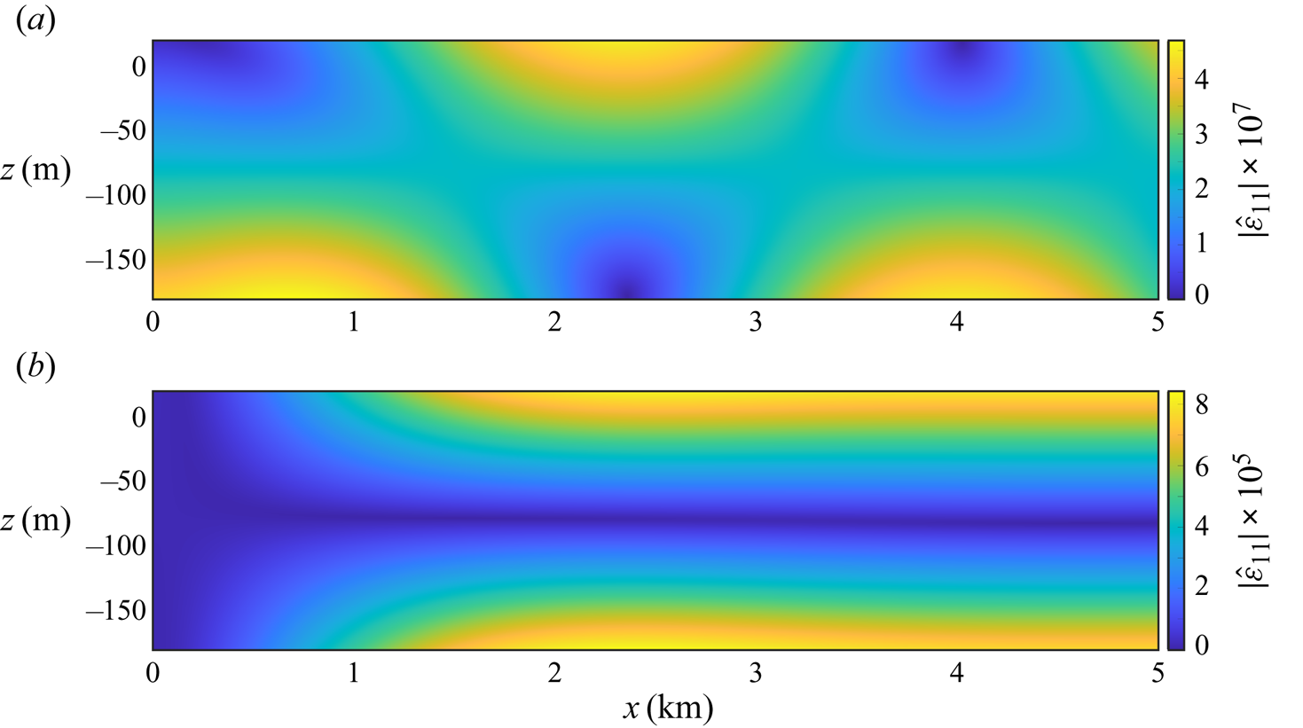
Example wave-induced strain profiles at the lower ice shelf surface (figure 5) show the influence of the additional terms in the thin-plate approximation. Results from the benchmark thin-plate model (without water–ice coupling at the shelf front and extensional waves) are shown alongside results from an intermediate version of the model derived in § 5 that includes water–ice coupling at the shelf front but no extensional waves, and the full model that includes extensional waves. The differences between the intermediate model (with water–ice coupling) and the full model (with extensional waves) highlight the influence of the extensional waves on the shelf strains. The differences between the benchmark model (in which hydrodynamic loads are imposed only at the lower shelf surface) and the two new models highlight the influence of hydrodynamic forcing at the shelf front on the shelf strains. In particular, the differences between the benchmark and intermediate models isolate the effects of water–ice coupling at the shelf front from the coupling at the lower surface on flexural waves. The strains are scaled by the shelf thickness, such that strains for different thickness values are of the same order of magnitude for the different wave periods. In all four cases (figure 5a–d), the benchmark model predicts the strain modulus increases from zero at the shelf front to a maximum value after several kilometres, followed by a plateau at a slightly smaller value.
Comparison of scaled wave-induced strain profiles predicted by three thin-plate models: (i) the benchmark model without water–ice coupling at the shelf front and extensional waves (Porter & Porter Reference Porter and Porter2004; Bennetts et al. Reference Bennetts, Biggs and Porter2007); (ii) an intermediate model in which water–ice coupling occurs at the shelf front through the velocity jump condition (5.21b) and the bending moment condition (5.26b); and (iii) the full model proposed in § 5 including extensional wave motion and water–ice coupling at the shelf front, for shelf thicknesses (a,c)  $h=200$ m and (b,d) $h=400$ m, and bed depth $H=800$ m, in response to incident waves with periods (a,b) $T=15$ s and (c,d) $T=50$ s.

For the shorter wave period (figure 5a,b), the addition of water–ice coupling at the shelf front (through (5.21b) and (5.26b)) causes a large relative increase in the strain, by factors of  ${\approx }3$ for the thinner shelf and ${\approx }75$ for the thicker shelf at the plateaus (approximately $x>3$ km). The strain at the shelf front is non-zero and, for the thicker shelf (figure 5b), the greatest strain occurs at the shelf front, such that the wave–ice coupling causes a qualitative change in the strain profile. The effect of wave–ice coupling on the strain profiles is almost imperceptible for the longer wave period (figure 5c,d), although the strains are one to two orders of magnitude larger than for the shorter period ( $h \vert \hat {\varepsilon }_{11}\vert$ is up to order $10^{-3}$ for $T=50$ s vs order $10^{-5}$– $10^{-4}$ for $T=15$ s). Moreover, the change in scale masks the similarity in the shelf front strain values for the respective thicknesses, as anticipated by the coupling coefficient in the bending moment condition (figure 3b; yellow curves).
The addition of extensional waves changes the qualitative behaviour of the strain profiles for the shorter wave period (figure 5a,b). Notably, the strain does not reach a constant value away from the shelf front, due to interference in the underlying wave field between the flexural wave (with wavenumber  $\kappa$) and the extensional wave ( $q$), both of which persist into the far field, $x\to \infty$. The extensional waves have a far smaller effect on the strain profiles for the longer wave period (figure 5c,d), although their influence for the thicker shelf (figure 5d) is greater than that of the water–ice coupling on the flexural waves.
The proportion of incident wave energy transmitted into the flexural and extensional waves is used to assess their relative influence on the ice shelf motion vs wave period. The distribution of incident wave energy is derived from (5.28), which gives the energy balance
 \begin{equation} \mathcal{R}+\mathcal{T}^{{(\,fl)}}+\mathcal{T}^{{(ex)}}=1, \end{equation}
where
 \begin{align} \mathcal{R}=\vert \mathcal{R}^{{(op \rightarrow op)}}\vert^{2} ,\quad \mathcal{T}^{{(\,fl)}}=\vert \mathcal{T}^{{(\,fx \rightarrow op)}}\vert\,\vert \mathcal{T}^{{(op \rightarrow fl)}}\vert \quad \text{and}\quad \mathcal{T}^{{(ex)}}=\vert \mathcal{T}^{{(ex \rightarrow op)}}\vert\,\vert \mathcal{T}^{{(op \rightarrow ex)}}\vert \end{align}
are the proportions of the incident energy in the reflected wave ( $\mathcal {R}$), and the flexural ( $\mathcal {T}^{{(\,fl)}}$) and extensional ( $\mathcal {T}^{{(ex)}}$) waves transmitted into the shelf–cavity region.
For periods in the majority of the swell regime (here defined as wave periods from 10 to 30 s), the transmitted extensional waves carry more energy than the flexural waves (figure 6). The difference is approximately an order of magnitude for the shortest periods considered, and is greatest for the thinner shelf (figure 6a). The proportion of energy in the flexural waves increases steeply as wave period transitions from the swell to infragravity regimes, whereas the proportion of energy in the extensional waves slightly decreases. This causes the flexural wave energy to exceed the extensional wave energy in the infragravity wave regime, with the difference approximately two orders of magnitude at the longest wave periods considered and greater for the thinner shelf. The wave period at which the energies of the flexural and extensional waves are equal is longer for the thicker shelf than the thinner shelf ( ${\approx }30$ s vs ${\approx }23$ s).
Transmitted energy proportions for flexural and extensional waves (blue and red curves, respectively) vs wave period, for shelf thicknesses (a)  $h=200$ m and (b) $h=400$ m, and bed depth $H=800$ m.

For the cases tested with the full approximation outlined in § 5, the maximum shelf strains due to incident waves are attained at either the upper or lower shelf surface, which is similar to the benchmark model, where the maximum strains are attained at both upper and lower surfaces due to symmetry about the mid-plane. In the swell regime, the maximum strains predicted by the full model far exceed those of the benchmark model (figure 7a,b). The maximum strains at the upper surfaces slightly exceed those at the lower surface for the smallest wave periods considered. For longer periods, the maximum strains at the upper and lower surfaces are almost identical, and they tend towards the maximum strain predicted by the benchmark model, as wave period increases, such that they are indistinguishable in the infragravity regime.
(a,b) Maximum flexural strains due to incident waves at the upper ( $z=h-d$) and lower ( $z=-d$) shelf surfaces, and (c,d) corresponding locations, for shelf thicknesses (a,c) $h=200$ m and (b,d) $h=400$ m, and bed depth $H=800$ m, with results of the benchmark model shown for reference.

For the shortest wave period considered, the strain maxima at the upper surface occur only hundreds of metres from the shelf front, and move closer towards the shelf front as wave period decreases (figure 7c,d). In contrast, the maxima predicted by the benchmark model occur more than a kilometre away from the shelf front, and the maxima at the lower surface predicted by the full approximation occur even farther away. For shorter periods and the thinner shelf, the strain maxima move between distinct regions of large strain at the upper and lower surfaces (yellow patches in figure 4a), which causes the jumps in the locations of maximum strain (figure 7c).
7. Conclusions and discussion
The governing equations for the canonical problem of incident waves from the open ocean forcing motions of a floating ice shelf, in which the ice shelf is modelled by the full equations of elasticity and has an Archimedean draught, have been derived from a variational principle. The variational principle was used to derive a thin-plate approximation for the ice shelf. Previous derivations of the governing equations for ice shelves (or other floating bodies) as thin floating elastic plates, including those based on variational principles (Porter & Porter Reference Porter and Porter2004; Bennetts et al. Reference Bennetts, Biggs and Porter2007), have assumed the thin-plate approximation from the outset (i.e. depth averaging in the ice), thus resulting in the ice shelf satisfying free edge conditions at the shelf front. In contrast, the variational principle presented in this study derives shelf front conditions in which the water and ice are coupled. The water–ice coupling allows extensional waves to be excited in the shelf, further extending previous thin-plate approximations. The thin-plate approximation was combined with a single-mode approximation in the water. Results have shown that the water–ice coupling at the submerged portion of the shelf front and the extensional waves significantly increase wave-induced shelf strains for wave periods in the swell regime. In contrast, they have a negligible effect for periods in the infragravity wave regime.
Variational principles are often used to derive approximations for water wave problems, dating back to Luke (Reference Luke1967), and with the so-called (modified) mild-slope equations of Miles (Reference Miles1991), Chamberlain & Porter (Reference Chamberlain and Porter1995) and others of particular relevance to the present study. The variational principle presented in § 3 can be viewed as an extension of the variational principle of Porter & Porter (Reference Porter and Porter2004) to incorporate the full equations of elasticity for the floating ice. However, there are notable differences in the approach used here, which is more closely aligned to the ‘unified theory’ of Porter (Reference Porter2020) for open-water waves. In particular, our use of a displacement potential in the water, for consistency with the unknown displacements in the ice, is a major departure from Porter & Porter (Reference Porter and Porter2004) and others before. Further, we include interfacial stresses in the variational principle, so that all matching conditions arise as natural conditions of the variational principle, and essential conditions do not have to be imposed. There is evidence from studies on cognate problems (without water–ice coupling at the ice edge and extensional waves) that the single-mode approximation is accurate (Bennetts et al. Reference Bennetts, Biggs and Porter2007; Bennetts, Biggs & Porter Reference Bennetts, Biggs and Porter2009; Bennetts & Meylan Reference Bennetts and Meylan2021). In particular, Liang, Pitt & Bennetts (Reference Liang, Pitt and Bennetts2023) give evidence the single-mode approximation is accurate for ice shelf strains across a range of relevant wave periods and for realistic geometries. However, in general, the single-mode approximation becomes less accurate as frequency increases and the impedance mismatch between the open water and the cavity water becomes more pronounced (figure 2). Following Bennetts et al. (Reference Bennetts, Biggs and Porter2007), the single-mode approximations (5.4) can be extended to include a finite number of vertical modes that support evanescent waves, such that continuities between the open ocean and sub-shelf water cavity are satisfied to an arbitrary accuracy.
The primary motivation for present study was to derive a consistent thin-plate approximation, in which the water and ice are coupled at the shelf front. Regimes have been found in which the water–ice coupling has a major impact on ice shelf strains. However, studies are still needed to test the validity of the thin-plate assumptions ((4.1) or similar), particularly for thick shelves and incident swell. The studies could be based on numerical solutions, for which the software presented by Kalyanaraman et al. (Reference Kalyanaraman, Meylan, Lamichhane and Bennetts2021) is available if the present model is modified to a finite length shelf and the gravitational acceleration in the shelf is removed. Alternatively, similarly to the approach proposed above to extend the single-mode approximation in water, the thin-plate ansatzes (4.1) could be extended with additional terms to improve accuracy. For instance, higher-order terms in the ansatz for the vertical displacement would remove an inconsistency between the low-order ansatz used in this study and the plane stress assumption (Fung Reference Fung1965). Therefore, the method outlined to derive the thin-plate approximation provides a framework to obtain the full solution (3.25) and (3.26).
The approximation derived in this study (§ 5) predicts extensional wave displacements that are greater than flexural wave displacements for low frequencies (long periods), and that the amplitude ratio becomes unbounded as frequency tends to zero, such that  $\mathcal {T}^{{(op \rightarrow ex)}} \to \infty$ as $\omega \to 0$ (not shown), which is consistent with the findings of Abrahams et al. (Reference Abrahams, Mierzejewski, Dunham and Bromirski2023). This property is a consequence of the elliptical trajectories of water particles having aspect ratios that increasingly skew towards the horizontal axis as wavelengths increase. However, our results show that extensional waves have a negligible impact on shelf strains for long periods (e.g. figure 5). Further, flexural waves hold greater energy than extensional waves for long periods, i.e. $\mathcal {T}^{(\,{fl})}\gg \mathcal {T}^{({ex})}$ for $T\gg 1$ (figure 6), where the small limiting values of $\mathcal {T}^{(\,{fl})}$ are due to decreases in $\mathcal {T}^{{(ex \rightarrow op)}}$ compensating for increases in $\mathcal {T}^{{(op \rightarrow ex)}}$. Intuitively, as incident waves get longer, the impact of the ice cover decreases, resulting in $\kappa \approx k$ (figure 2) and most of the incident wave transmitting into a flexural-gravity wave in the shelf–cavity interval ( $\mathcal {T}^{{(op \rightarrow ex)}}\approx 1$).
The strain magnitudes presented in § 6 are one to two orders of magnitude smaller for wave periods in the swell regime than in the infragravity wave regime. However, swell amplitudes are typically much greater than infragravity wave amplitudes, such that the benchmark model predicts they create strains of comparable magnitude (Bennetts, Liang & Pitt Reference Bennetts, Liang and Pitt2022). In particular, flexural-gravity waves at periods in the swell regime are amplified by crevasses in ice shelves (Bennetts et al. Reference Bennetts, Liang and Pitt2022), and, thus, our findings highlight a potential, additional role of water–ice coupling and extensional waves in these amplifications. Further, the thin-plate model presented could be extended to study whether periodic thickness variations in the ice shelf block ocean wave energy propagation through the shelf (Freed-Brown et al. Reference Freed-Brown, Amundson, MacAyeal and Zhang2012; Nekrasov & MacAyeal Reference Nekrasov and MacAyeal2023).
The dynamic problem ( $\omega \neq 0$) was considered in this study, so that the derived approximation could be compared with the benchmark thin-plate approximation, in order to identify the influence of water–ice coupling at the shelf front and extensional waves. The static problem ( $\omega =0$) can also be derived from the variational principle (Appendix B). Static extensions are forced by traction at the shelf front (B2c), due to atmospheric pressure and static water pressure (B3). The shelf front condition indicates the extensional contribution to the non-zero strain is $u'(0)=-p_{0} / G$, which is order $10^{-5}$ for $h=200$ m and 400 m. It is comparable to the dynamic strains induced by infragravity waves (figure 5c,d) and one to two orders of magnitude greater than the dynamic strains induced by swell (figure 5a,b), although these are only for one metre amplitude incident waves and mean daily swell amplitudes reaching ice shelves can be up to four–five times larger (Teder et al. Reference Teder, Bennetts, Reid and Massom2022). However, bounded static extensions require a finite shelf (B6). In contrast, the semi-infinite shelf supports bounded static flexure (B5) forced by bending at the shelf front (B2a) due to static water pressure (B3). The flexural contribution to the non-zero strain is $(z+d-h / 2) w''(0)=(z+d-h / 2)\,p_{1} / F$, which has a maximum value at $z=-d$ on the order of $10^{-5}$ for $h=200$ m and $10^{-4}$ for $h=400$ m. Therefore, the static problem indicates the static strains close to the ice edge can be comparable to or larger than the dynamic strains caused by wave motion. This may motivate future studies to consider interactions between the static and dynamic problems, i.e. pre-stress. Pre-stress on the relatively short time scales of ocean waves could also result from long time scale viscous creep (e.g. Weertman Reference Weertman1957).
Acknowledgements
We thank the anonymous referees for their insightful comments.
Funding
L.G.B. is funded by Australian Research Council grants FT190100404 and DP200102828. T.D.W. was supported by Schmidt Futures – a philanthropic initiative that seeks to improve societal outcomes through the development of emerging science and technologies.
Declaration of interests
The authors report no conflict of interest.
Appendix A. Finite deformation of an infinitely long ice shelf
Consider an infinitely long ice shelf of constant density  $\rho _{{i}}$ in the absence of gravity. Let gravity be increased from zero, such that it compresses the ice shelf onto an incompressible water base. This induces a finite initial stress (typically called a ‘pre-stress’) to the ice, which can modify the properties of waves in the ice.
In Eulerian coordinates (relative to the ice shelf after being compressed), the strain tensor is  $\boldsymbol {\varepsilon }^{{finite}}$, with components (Spencer Reference Spencer2004)
 \begin{equation} \varepsilon^{{finite}}_{ij} = \varepsilon_{ij} -\frac12\sum_{k=1}^{3}U_{k,x_{i}} U_{k,x_{j}}, \end{equation}
where  $\varepsilon _{ij}$ is the linearised strain tensor from (2.4). In order to consider infinitesimal waves in the $x$–
$x$– $z$ plane, the displacement is split, such that
 \begin{equation} U_{1}(x,z,t)=\hat{U}(x,z,t), \quad U_{2}(x,z,t)=W^{{hs}}(z) + \hat{W}(x,z,t) \quad\text{and}\quad U_{3}=0, \end{equation}
where the superscript ‘ $hs$’ indicates hydrostatic displacements and hats indicate dynamic displacements due to waves. Substituting (A2a–c) into (A1), and ignoring second-order terms involving $\hat {U}_i$, the strain is split into
 \begin{equation} \boldsymbol{\varepsilon}^{{finite}}(x,z,t) = \boldsymbol{\varepsilon}^{{hs}}(z) + \hat{\boldsymbol{\varepsilon}}(x,z,t), \end{equation}
where
 \begin{equation} \varepsilon^{{hs}}_{22} = W^{{static}}_{z} \left(1 -\frac{1}{2} W^{{static}}_z\right) \quad\text{and}\quad \hat{\boldsymbol{\varepsilon}} = \frac12\begin{pmatrix} 2 \hat{U}_x & 0 & \hat{U}_{z} + \gamma \hat{W}_{x}\\ 0 & 0 & 0\\ \hat{U}_{z} + \gamma \hat{W}_{x} & 0 & 2 \gamma \hat{W}_{z} \end{pmatrix}, \end{equation}
in which
 \begin{equation} \gamma(z)=1-W^{{hs}}_z \quad\text{and}\quad \varepsilon^{{hs}}_{ij}=0 \quad\text{if}\ i\neq2 \quad\text{or}\ j\neq2 \quad (i,j\in\{1,2,3\}). \end{equation}
The factor  $\gamma$ induces coupling between the static and wave problems. The density after compression is $\rho _{{i}} \gamma (z)$, i.e. it is no longer constant. However, if $W^{{hs}}_z \ll 1$, $\gamma \approx 1$, hence the coupling between the static and wave problems is removed and the ice has constant density.
While the finite-deformation problem in this case is tractable, it is simpler and more instructive to solve the linear problem and check the size of  $W^{{hs}}_z$ a posteriori. From (3.25) and (3.26), the static problem can be written
 $$\begin{gather} \sigma^{{hs}}_{22,z} = \rho_{{i}} g, \end{gather}$$
 $$\begin{gather}\sigma^{{hs}}_{22} = M W^{{hs}}_{z}, \end{gather}$$
 $$\begin{gather}\sigma_{22}^{{hs}}(h-d) + \rho_{{i}} g W^{{hs}}(h-d) =-P_{{at}}, \end{gather}$$
 $$\begin{gather}W^{{hs}}(-d) = 0, \end{gather}$$
where
 \begin{equation} M = \frac{E (1-\nu)}{(1+\nu) (1-2\nu)} \end{equation}
is the  $P$-wave modulus, which is typically $10^9$– $10^{10}$ Pa. Hence
 $$\begin{gather} \sigma^{{hs}}_{22} = M W^{{hs}}_z = \rho_{{i}} g (z+d) + S_{{bt}}^{{hs}} \in[S_{{bt}}^{{hs}},S_{{bt}}^{{hs}}+\rho_{{i}} g h], \end{gather}$$
 $$\begin{gather}\text{and}\quad M W^{{hs}} = \tfrac12 \rho_{{i}} g (z+d)^2 + S_{{bt}}^{{hs}} (z+d), \end{gather}$$
where  $S_{{bt}}^{{hs}}$ is the unknown stress at the bottom of the ice. Here, $W^{{hs}}$ satisfies (A6d), while (A6c) is satisfied if
 \begin{equation} -\frac{S_{{bt}}^{{hs}}}{M}=\frac{2 P_{{at}} + \rho_{{i}} g h (2 M + \rho_{{i}} g h)}{2 M (M + \rho_{{i}} g h)} = max\{|W_z^{{hs}}|\quad\text{for } z\in[-d,h-d]\}. \end{equation}
Since the atmospheric pressure  $P_{{at}}\approx 10^6$ Pa, $|W^{{hs}}_z|\ll 1$ if the ice thickness $h\ll M/(\rho _{{i}}g)\approx 5\times 10^5$ m or 500 km. Hence, for typical ice shelves, gravitational compression should have only a negligible effect on wave motion.
Appendix B. Static version of thin-plate equations ( $\omega =0$)

The static versions ( $\omega =0$) of the thin-plate equations (5.12a,c) are, respectively,
 \begin{equation} F w'''' + w = 0 \quad\text{and}\quad u''=0 \quad\text{for } x>0. \end{equation}
The corresponding static versions of the shelf front conditions (5.26a–c) are
 \begin{equation} F w'' - p_{1} =0, \quad w''' =0 \quad\text{and}\quad G\, u' + p_{0} = 0 \quad\text{for } x=0, \end{equation}
where
 \begin{align} p_{0} & = \frac{1}{\rho_{{w}} g} \left\{ \int_{-d}^{0}(P_{{at}} + \rho_{{w}}g z)\,\mathrm{d} z + \int_{0}^{h-d}P_{{at}} \,\mathrm{d} z\right\}\nonumber\\ & = \frac{P_{{at}} h}{\rho_{{w}} g} - \frac{d^{2}}{2} , \end{align}
 \begin{align} \text{and}\quad p_{1} & = \frac{1}{\rho_{{w}} g} \left\{ \int_{-d}^{0}\left(d-\frac{h}{2}+z\right) (P_{{at}} + \rho_{{w}}g z)\,\mathrm{d} z +\int_{0}^{h-d}\left(d-\frac{h}{2}+z\right) P_{{at}} \,\mathrm{d} z \right\}\nonumber\\ & =-\frac{d^{2}}{2} \left(\frac{d}{3}-\frac{h}{2}\right)\!. \end{align}
 The static flexure,  $w=w_{{st}}$, satisfying (B1a), has bounded solutions of the form
 \begin{equation} w_{{st}}(x) = \mathrm{e}^{-\beta x} (C_+\,\mathrm{e}^{\mathrm{i} \beta x} +C_-\,\mathrm{e}^{-\mathrm{i} \beta x}), \end{equation}
where  $\beta = (4 F)^{-1/4}$ and $C_{\pm }$ are determined from (B2a,b). The general solution for the static extension, $u=u_{{st}}$, satisfying (B1b) is
 \begin{equation} u_{{st}}(x) = A x+B. \end{equation}
It has no bounded solutions satisfying the shelf front condition (B2c).


 Open access