


1. Introduction
The spatio-temporal processes by which background fluid is transported and mixed into a turbulent flow are collectively known as entrainment. Entrainment of mass leads to the expansion of the turbulent flow into the background, hence it is critical in defining the behaviour of numerous important phenomena ranging from the growth of turbulent boundary layers (Chauhan et al. Reference Chauhan, Philip, De Silva, Hutchins and Marusic2014) to meteorological phenomena such as cloud growth/decay in both terrestrial and extra-terrestrial environments (Atreya et al. Reference Atreya, Wong, Owen, Mahaffy, Niemann, de Pater, Drossart and Encrenaz1999; de Rooy et al. Reference de Rooy, Bechtold, Fröhlich, Hohenegger, Jonker, Mironov, Pier Siebesma, Teixeira and Yano2013). It is governed by small-scale turbulent dynamics within an interfacial layer adjacent to the outermost boundary between the two regions of fluid. In the special case where the background fluid is non-turbulent, this layer is known as the turbulent/non-turbulent interface (TNTI). More generally, the background fluid is itself turbulent (e.g. the cloud-containing atmosphere), in which case this layer is known as the turbulent/turbulent interface (TTI).
The TNTIs, and entrainment from a non-turbulent background, have been studied for many years (Zeldovich Reference Zeldovich1937; Corrsin & Kistler Reference Corrsin and Kistler1955). Entrainment is a multi-scale process (Mistry et al. Reference Mistry, Philip, Dawson and Marusic2016), but in general large-scale processes, in which packets of background fluid are ingested into the flow, are termed ‘engulfment’ whilst small-scale processes, dominated by viscous diffusion, are termed ‘nibbling’. Intermediate length scales are introduced through the contortion of the TNTI, into a fractal shape (Sreenivasan & Meneveau Reference Sreenivasan and Meneveau1986), by turbulent motions within the flow thereby enhancing the surface area over which nibbling occurs. Existing work has shown that in regions of turbulent flows dominated by large-scale coherent motions, e.g. the near field of a turbulent mixing layer, engulfment is dominant (Yule Reference Yule1978) whilst in regions of more fully developed turbulence, e.g. the far field of a jet, nibbling is dominant (Westerweel et al. Reference Westerweel, Fukushima, Pedersen and Hunt2005).
Far less research has been conducted on TTIs and entrainment from a turbulent background. Until recently, zeroth-order questions such as ‘Whether the presence of background turbulence enhances or diminishes entrainment rate in comparison to a non-turbulent background?’, and ‘Whether TTIs even existed in scenarios in which the turbulence intensity of the background and primary flow were similar (da Silva et al. Reference da Silva, Hunt, Eames and Westerweel2014)?’ remained unanswered. The existence of TTIs, even in scenarios in which the background turbulence intensity is greater than in the primary flow, has now been verified (Kankanwadi & Buxton Reference Kankanwadi and Buxton2020). A turbulent background has also now been shown to suppress entrainment rate, with respect to a non-turbulent background, in the far field of a turbulent wake, where nibbling is the dominant entrainment mechanism (Kankanwadi & Buxton Reference Kankanwadi and Buxton2020), and to enhance the entrainment rate in the near field, where engulfment is a significant, if not the dominant, entrainment mechanism (Kankanwadi & Buxton Reference Kankanwadi and Buxton2023).
The physics of TTIs have also been shown to be different from those for TNTIs. As first postulated by Corrsin & Kistler (Reference Corrsin and Kistler1955), and subsequently verified many years later (Holzner et al. Reference Holzner, Liberzon, Nikitin, Kinzelbach and Tsinober2007), the physics at the outermost surface of a TNTI are dominated by viscous diffusion, whilst in the inner portion of the TNTI, the so-called turbulent buffer layer (Van Reeuwijk & Holzner Reference Van Reeuwijk and Holzner2013), they are dominated by inertial vorticity stretching. Contrastingly, in a TTI, viscous diffusion is negligible throughout the TTI, with vorticity stretching being responsible for producing the discontinuity in enstrophy/vorticity magnitude (Kankanwadi & Buxton Reference Kankanwadi and Buxton2022) characteristic of a TTI (Kankanwadi & Buxton Reference Kankanwadi and Buxton2020). Studies have also shown that the presence of background turbulence makes the TTI more convoluted than a TNTI (Kankanwadi & Buxton Reference Kankanwadi and Buxton2020; Kohan & Gaskin Reference Kohan and Gaskin2022; Chen & Buxton Reference Chen and Buxton2023).
The above work has focused on the entrainment of mass from the background, whether turbulent or not, but other quantities such as enstrophy, enthalpy, scalar, buoyancy, etc. can also be entrained across a TNTI/TTI. In this paper we focus on the entrainment of momentum, in particular the (dominant) streamwise component of momentum, and kinetic energy from a turbulent background. Entrainment of momentum, when considering a suitable control volume encompassing a wake-generating body, is closely related to the drag, whilst the entrainment of kinetic energy from geostrophic wind into the atmospheric boundary layer, for example, is important in meteorological phenomena. In the subsequent section, we consider the relative ‘efficiencies’ of the entrainment fluxes of momentum and kinetic energy relative to the mass flux for a wake exposed to a turbulent background.
2. Theoretical development
Let us consider a planar wake exposed to both a turbulent and non-turbulent background. In particular, we interrogate a portion of the TTI/TNTI within a plane over a streamwise extent of  $L_x$. We introduce a local coordinate system
  $(\xi _s, \xi _n)$, which defines the interface-tangential and interface-normal directions, respectively, such that the outermost boundary of the interface (the irrotational boundary for the TNTI) is defined as
  $\xi _n = 0$. Having done so, we can now define the entrainment fluxes of mass
  $\dot M$, the streamwise component of momentum
  $\dot P_x$ and kinetic energy
  $\dot K$ for an incompressible fluid by integrating along the temporally evolving length of the outermost boundary of the TTI/TNTI,
  $\ell '(t)$, that is captured in the domain of streamwise extent
  $L_x$:
 \begin{gather} \dot M = \frac 1T \int_0^{T} \left(\int_{\ell'(t)} \rho v_e(\xi_s)\,{\textrm d} \xi_s\right) {\textrm d} t =: \overline{\int_{\ell'} \rho v_e \,{\textrm d} \xi_s} , \end{gather}
 \begin{gather}\dot P_x = \overline{\int_{\ell'} \rho U v_e\,{\textrm d} \xi_s} , \end{gather}
 \begin{gather}\dot K = \frac 12 \overline{\int_{\ell'} \rho ( U^2 + V^2 ) v_e \,{\textrm d} \xi_s} . \end{gather}
Here, the entrainment velocity  $v_e$ is the relative velocity between the outer surface of the TTI/TNTI and the fluid in a direction normal to the tangent of the TTI/TNTI (Holzner & Lüthi Reference Holzner and Lüthi2011), and
  $U = U(\xi _n = 0)$ and
  $V = V(\xi _n = 0)$ are the streamwise and transverse (in standard Cartesian
  $(x,y)$ directions) components of the velocity at the outermost boundary of the TTI/TNTI.
Let us now consider entrainment of these various quantities from a non-turbulent background with uniform free-stream velocity  $U_\infty$. Owing to the presence of vorticity on the turbulent side of the TNTI, and the irregular shape of the interface, irrotational velocity fluctuations are observed on the non-turbulent side (Holzner et al. Reference Holzner, Lüthi, Tsinober and Kinzelbach2009). We thus add this irrotational fluctuation to the free-stream velocity such that at
  $\xi _n = 0$ we have
  $U = U_\infty + \tilde u$ and we note that
  $V = \tilde v$ under the mild assumption that the wake is spreading slowly (via entrainment) with respect to
  $U_\infty$. The entrainment flux of momentum now becomes
 \begin{equation} \dot P_x = \rho \overline{\int_{\ell'} (U_\infty + \tilde u) v_e \,{\textrm d} \xi_s} \approx \rho \ell \langle (U_\infty + \tilde u) v_e \rangle , \end{equation}
where  $\langle \,\cdot \, \rangle$ denotes spatio-temporal ensemble averaging along the outermost boundary of the TNTI within the interrogation domain of streamwise extent
  $L_x$, and
  $\ell = \overline {\ell '}$ with
  $\ell '$ being the (temporally) fluctuating length of the TNTI over the domain as before.
This last approximation arises from the assumption that the instantaneous length of the interface within the interrogation domain  $\ell '$ does not in any way affect
  $(U_\infty + \tilde u)v_e$. The credibility of this assumption is tested empirically and presented in § 4. We are now left with
 \begin{equation} \dot P_x \approx \rho \ell U_\infty \langle v_e \rangle + \rho \ell \langle \tilde u v_e \rangle . \end{equation}
The entrainment velocity  $v_e$ is a turbulent velocity that is known to scale with a viscous velocity scale (Holzner & Lüthi Reference Holzner and Lüthi2011; Zhou & Vassilicos Reference Zhou and Vassilicos2017) and is hence focused at high wavenumbers. Contrastingly,
  $\tilde u$ is an irrotational fluctuation driven by irrotational strain/pressure fluctuations (Holzner et al. Reference Holzner, Lüthi, Tsinober and Kinzelbach2009) induced by the contortion of the TNTI. Since the TNTI is fractal, with this fractal geometry focused in the inertial range of scales, these contortions are likely to drive velocity fluctuations focused at lower (inertial) wavenumbers, hence we expect the correlation
  $\langle \tilde u v_e \rangle \approx 0$, leaving us with
  $\dot P_x \approx \rho \ell U_\infty \langle v_e \rangle$. Noting that
 \begin{equation} \dot M = \rho \overline{\int_{\ell'} v_e\,{\textrm d} \xi_s} \approx \rho \ell \langle v_e \rangle , \end{equation}
we see that  $\dot P_x \approx U_\infty \dot M$. Similar analysis yields
  $\dot K \approx \frac 12 U_\infty \dot P_x \approx \frac 12 U_\infty ^2 \dot M$, i.e. there is a direct proportionality between the entrainment fluxes of momentum and kinetic energy and that of mass when the background is an idealised non-turbulent flow.
Let us now apply similar analysis to entrainment into a planar wake exposed to a turbulent background with mean free-stream velocity of  $U_\infty$ such that
  $U = U(\xi _n = 0) = U_I + u'$ and
  $V = V(\xi _n = 0) = v'$, again under a similarly mild assumption that the mean wake spreading rate is small. Here,
  $U_I = \langle U \rangle \approx U_\infty$ is the ensemble-averaged velocity at
  $\xi _n = 0$, i.e. the outermost boundary of the TTI. Note also that the velocity fluctuations
  $(u',v')$ here may in general comprise both standard turbulent fluctuations as well as fluctuations caused by the contortion of the TTI, similarly to the irrotational free-stream perturbations caused by a TNTI, although this is a minor detail. The entrained turbulent momentum flux is given by
 \begin{equation} \dot P_x = \rho \overline{\int_{\ell'} (U_I + u') v_e \,{\textrm d} \xi_s} \approx \rho \ell U_I \langle v_e \rangle + \rho \ell \langle u' v_e \rangle , \end{equation}
under the same assumptions as before.
We note that for different ‘flavours’ of background turbulence, as parametrised by  $\{ \mathcal {L}, k \}$, where
  $\mathcal {L}$ is the integral length scale and
  $k$ is the turbulence intensity of the background turbulence, the tortuosity of a TTI has been shown to be
  $\tau = \ell / L_x = \tau (\mathcal {L}, k)$ (Kankanwadi & Buxton Reference Kankanwadi and Buxton2020; Kohan & Gaskin Reference Kohan and Gaskin2022). Nevertheless, when considering a particular ‘flavour’, i.e. fixed
  $\{ \mathcal {L}, k \}$, we still assume
  $\ell '$ to have little effect on
  $v_e$ and
  $u' v_e$, an assumption that is empirically tested in § 4. This leaves us with
 \begin{equation} \dot P_x \approx U_I \dot M + \rho \ell \langle u' v_e \rangle . \end{equation}
We thus observe that the correlation  $\langle u' v_e \rangle$ determines the relative ‘efficiency’ of the entrainment of momentum to the entrainment of mass. When
  $\langle u' v_e \rangle = 0$, then the relative efficiency for the entrainment of momentum to mass is identical across a TTI to that across an idealised TNTI, with a direct proportionality between
  $\dot P_x$ and
  $\dot M$.
Note, however, that the presence of background turbulence is shown to affect entrainment, i.e.  $\dot M = \dot M(\mathcal {L}, k)$ (Kankanwadi & Buxton Reference Kankanwadi and Buxton2020, Reference Kankanwadi and Buxton2023), which will therefore affect the entrainment rate of momentum itself if not the relative efficiency of the entrainment of momentum to mass. Conversely, in a turbulent background when
  $\langle u' v_e \rangle \neq 0$, this direct proportionality between
  $\dot P_x$ and
  $\dot M$ is broken. When
  $\langle u' v_e \rangle > 0$, momentum is entrained more efficiently than mass, and for
  $\langle u' v_e \rangle < 0$, it is entrained less efficiently than mass, relative to an idealised non-turbulent background. Note that
  $v_e > 0$ is defined to be entrainment and
  $v_e < 0$ to be detrainment (mass ejected from the wake into the background).
We may perform similar analysis for the entrainment of kinetic energy, again making the mild assumption that  $V = v'$ since the wake is spreading slowly, and a similar assumption relating to
  $\ell '$ not affecting
  $v_e$ or the correlation between
  $v_e$ and fluctuating velocity components
  $u'$ and
  $v'$:
$v'$:
 \begin{align} \dot K &= \frac \rho 2 \overline{\int_{\ell'} [(U_I + u')^2 + v'^2 ] v_e \, {\textrm d} \xi_s} \end{align}
 \begin{align} &\approx \frac{\rho \ell}{2} ( U_I^2 \langle v_e \rangle + 2 U_I \langle u' v_e \rangle + \langle u'^2 v_e \rangle + \langle v'^2 v_e \rangle ) \end{align}
 \begin{align} &= \frac 12 U_I^2 \dot M + \frac{\rho \ell}{2} [ 2U_I \langle u' v_e \rangle + \langle u'^2 v_e \rangle + \langle v'^2 v_e \rangle ] . \end{align}
As previously, we notice that the correlations appearing in the square brackets of (2.11) determine whether kinetic energy is entrained more or less ‘efficiently’ than mass, relative to an idealised non-turbulent background. Further, should  $\langle u' v_e \rangle \neq 0$, then comparison of (2.8) and (2.11) shows that the relative efficiency of the entrainment of kinetic energy to momentum is also broken (with respect to this efficiency across an idealised TNTI) by the presence of background turbulence.
3. Experimental methods
The experimental configuration was similar to that of Chen & Buxton (Reference Chen and Buxton2023) in which a circular cylinder of diameter  $D = 10$ mm was exposed to various ‘flavours’/cases of grid-generated background turbulence. The cylinder and the grid were mounted in the hydrodynamics flume of the Department of Aeronautics at Imperial College London and the water depth was set such that the flow's cross-section was
  $0.6~{\rm m} \times 0.6~{\rm m}$. The water speed was
  $U_\infty = 0.38$ m s
 $^{-1}$, hence the Reynolds number based on the cylinder diameter was
  $Re_D \approx 3.8 \times 10^3$. Both the length scale
  $\mathcal {L}$ and intensity
  $k$ of the background turbulence were independently varied, where
 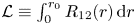 $\mathcal {L} \equiv \int _0^{r_0} R_{12}(r)\, {\textrm d} r$ in which
  $R_{12}(r)$ is the correlation between
  $u'(x,y)$ and
  $u'(x, y+r)$ integrated to the first zero-crossing
  $r_0$, and
  $k \equiv \sqrt {\overline {(u'^2 + v'^2)/2}}/U_\infty$, based on our two-dimensional velocity data. This was achieved by using a combination of regular and fractal turbulence-generating grids and altering the grid–cylinder streamwise separation, similarly to Chen & Buxton (Reference Chen and Buxton2023). Figure 1(a) outlines the parametric envelope of this campaign at the equivalent position of
  $x/D = 20$ but in the absence of the cylinder. Runs are split into three groups based on the background turbulence intensity
  $k$; group 1 is most similar to the no-grid case, whereas
  $k > k_{wake}$ for group 3.
(a) Envelope of background turbulence parameter space  $\{\mathcal {L}, k\}$ for the various test cases. (b) Locations of the measurement stations, centred on
  $x/D=(6.5, 10, 20, 30, 40)$ superimposed on a PLIF image (from Chen & Buxton Reference Chen and Buxton2023) illustrating the development of the wake exposed to case 2a background turbulence. The strip colours correspond to the symbols in figures 3 and 4.

Simultaneous particle image velocimetry (PIV) and planar laser-induced fluorescence experiments (PLIF) were conducted. We measured the entrainment fluxes of mass, momentum and kinetic energy at five different measurement stations centred on  $x/D = (6.5, 10, 20, 30, 40)$ downstream of the rear face of the cylinder. Each measurement station had a fixed streamwise extent
  $L_x = 3D$. Results from our previous work indicate that near-wake effects are particularly important for
  $x/D \lesssim 15$ (Chen & Buxton Reference Chen and Buxton2023). These measurement stations encompass the near wake,
  $x/D = (6.5,10)$, where engulfment is expected to be significant, and the far wake,
  $x/D = (30,40)$, where engulfment becomes negligible and nibbling dominates (Westerweel et al. Reference Westerweel, Fukushima, Pedersen and Hunt2005). The measurement station
  $x/D = 20$ is thus in some sense an intermediate measurement station where the flow transitions from one dominated by near-wake effects to one dominated by far-wake effects. Their positions are illustrated in figure 1(b).
Using classical methods to identify TNTIs, such as using vorticity magnitude (Bisset, Hunt & Rogers Reference Bisset, Hunt and Rogers2002) or turbulent kinetic energy thresholds (Chauhan et al. Reference Chauhan, Philip, De Silva, Hutchins and Marusic2014), is not viable since rotational/turbulent fluid is available on both sides of a TTI. Instead, a high-Schmidt-number scalar in the form of rhodamine 6G was released from the rear face of the cylinder, ensuring that molecular diffusion occurs over a vanishingly small length scale and hence the scalar acts as a faithful fluid marker. A single hole was used to release the scalar, which was introduced into the flow isokinetically using a Bürket micro-dosing unit 7615 connected via a 2 m long cable to the release point, ensuring that the discrete behaviour of the pump was smoothed out. Tests were conducted in a non-turbulent background examining the very near field of the wake and comparing the extent of the scalar to the enstrophy distribution. These tests confirmed that the released scalar was well stirred and faithfully marked the full extent of the wake (Kankanwadi & Buxton Reference Kankanwadi and Buxton2020), thereby allowing the PLIF camera to successfully capture the location of the TNTI/TTI. Interface identification was then achieved by using a threshold on the modulus of the captured light intensity gradient,  $\lvert \boldsymbol {\nabla } \phi \rvert$. A similar strategy was used in Kankanwadi & Buxton (Reference Kankanwadi and Buxton2020) and was shown to work effectively. Near-Kolmogorov-scale (
 $\eta$) PIV spatial resolution is required to resolve the fine-scale interfacial turbulence; this ranged from
  $1.7\eta$ to
  $3.2\eta$, which is comparable to the resolution of a direct numerical simulation.
The entrainment mass flux was computed via integrating  $v_e$ over the streamwise extent
  $L_x$ of the PIV field of view (Mistry et al. Reference Mistry, Philip, Dawson and Marusic2016; Kankanwadi & Buxton Reference Kankanwadi and Buxton2020) (cf. (2.1)). This process is outlined in figure 2. The approach was modified to include the local streamwise component of the fluid velocity at
  $\xi _n = 0$ to compute the entrained momentum flux (cf. (2.2)), and both the streamwise and transverse fluid velocities at
  $\xi _n = 0$ to compute the entrained kinetic energy flux (cf. (2.3)). Data were acquired for a period of
  $T = 25$ s, corresponding to approximately 200 periods of vortex shedding, at a measurement frequency of 200 Hz. Here
  $T$ corresponds to the averaging period of (2.1)–(2.3). The fixed (in absolute terms) streamwise extent of the field of view,
  $L_x = 3D$, varied from
  $147 \eta$ (case 1a,
  $x/D = 40$) to
  $326 \eta$ (case 3a,
  $x/D = 6.5$), where
  $\eta$ is the Kolmogorov length scale as directly computed along the outermost boundary of the TTI/TNTI (i.e. at
  $\xi _n = 0$) for the various cases of background turbulence tested and at the various measurement stations. Further,
  $L_x$ ranged between 1.25 and 8.8 integral scales of the background turbulence.
Graphical representation of the calculation of entrainment velocity  $v_e$. The process is illustrated for case 2b. (a) Identification of the TTI location (from the PLIF images) at times
  $t$ and
  $t + {\rm \Delta} t$, and superimposed onto the vorticity fields
  $\omega _z$ (from the PIV velocity fields). (b) Identified TTI positions at times
  $t$ (black line) and
  $t+{\rm \Delta} t$ (blue dashed line); and local fluid velocity (red arrows) from the PIV velocity fields along TTI identified at time
  $t+{\rm \Delta} t$. (c) TTI at time
  $t+{\rm \Delta} t$ advected backwards in time by the local fluid velocity (blue dashed line). (d) Close-up of (c) with displacement
  $\delta = v_e {\rm \Delta} t$ between TTI at time
  $t$ (black line) and the backwards-advected TTI at time
  $t + {\rm \Delta} t$ (blue dashed line) denoted with red arrows. Further details are presented in Kankanwadi & Buxton (Reference Kankanwadi and Buxton2020).

4. Results
The entrained momentum and kinetic energy fluxes are plotted against the entrained mass flux in figure 3(a). The measurements from case 1a, for the non-turbulent background, are denoted with a  $+$ sign. We first observe that all entrainment fluxes monotonically diminish with streamwise distance for the non-turbulent background cases. As the turbulent wake approaches the fully developed state, the large-scale coherent motions embedded within the wake decay (see figure 1b), leaving nibbling as the predominant entrainment mechanism. Assuming that the tortuosity of the TNTI approaches a fully developed state,
  $\tau \rightarrow \text {const.}$, then
 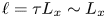 $\ell = \tau L_x \sim L_x$. Similarly, previous work has shown that
  $v_e \sim u_\eta$ (Holzner & Lüthi Reference Holzner and Lüthi2011), hence we can deduce that
  $\dot M \sim L_x u_\eta$. The similarity in the normalised mass entrainment fluxes in figure 3(c) for case 1a at
  $x/D = 30$ and
  $40$ attest to this scaling, and give us confidence in our measurements. Further, for the no-grid (TNTI) case 1a, all measurement stations with the exception of one obey the relationships that we previously derived for an idealised non-turbulent background, namely
  $\dot P_x = U_\infty \dot M$ and
 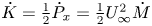 $\dot K = \frac 12 \dot P_x = \frac 12 U_\infty ^2 \dot M$. This provides empirical evidence to validate our assumption that
  $\ell$ may be taken outside of the spatio-temporal averaging of
  $\langle (U_\infty + \tilde u) v_e \rangle$ in (2.4) and that the correlation
  $\langle v_e \tilde u \rangle \approx 0$. The one exception is the entrained kinetic energy flux at
  $x/D = 6.5$, which will be discussed subsequently.
(a) Streamwise momentum entrainment flux  $\dot P_x$ (top line) and kinetic energy entrainment flux
  $\dot K$ (bottom line) plotted against entrainment mass flux
  $\dot M$. Symbols of the same shape/colour correspond to different cases of background turbulence, as defined in figure 1(a), at the same measurement station. (b,c) Plots of (b)
  $\dot M$ normalised with fixed velocity scale
  $U_\infty$ and (c)
  $\dot M$ normalised with the local Kolmogorov velocity scale at the outermost boundary of the TNTI/TTI
  $u_\eta (\xi _n = 0)$ for the various cases studied. Note that panel (c) can be cross-referenced against panel (a) to identify the various cases at the various measurement stations.

We observe the same general trend for a monotonic diminution in the entrainment fluxes with streamwise distance for the cases with a turbulent background. However, the picture is more complicated than for case 1a since, for example, in some cases the entrainment fluxes at  $x/D = 40$ are similar to those at
  $x/D = 20$ for others. Figures 3(b) and 3(c) show
  $\dot M$ for the various cases studied normalised by constant velocity scale
  $U_\infty$ (figure 3b) and by
  $u_\eta (\xi _n = 0)$, the local Kolmogorov velocity scale at the outermost boundary of the TTI/TNTI (figure 3c). In the far wake (
 $x/D \geq 30$), it can be seen that the entrained mass flux decreases as a function of
  $k$ (
$k$ ( $\text {group 3} < \text {group 2} < \text {group 1}$), confirming the results of Kankanwadi & Buxton (Reference Kankanwadi and Buxton2020), whereas in the near wake
  $\mathcal {L}$ also appears to play a role, with case 1c and in particular case 2b (those with the highest
  $\mathcal {L}$) seeing enhanced entrainment fluxes.
Importantly, we observe close agreement between the relative efficiencies of the entrainment of momentum/kinetic energy to mass across both TTIs and TNTIs. For all cases and at all measurement stations, almost no scatter from the line  $\dot P_x = U_I \dot M$, derived for entrainment from an idealised non-turbulent background, is observed. The picture is similar when considering the relative efficiency of the entrainment of kinetic energy to mass, with little scatter from the line
  $\dot K = \frac 12 U_I^2 \dot M$ from
  $x/D \geq 20$. Note, however, that figures 3(b) and 3(c) show that the presence of background turbulence does affect the mass entrainment rate, which is also spatially developing, i.e.
  $\dot M = \dot M(\mathcal {L}, k, x/D)$. Whilst the idealised ‘efficiency’ with which momentum/kinetic energy are entrained with respect to mass is preserved for a turbulent background beyond the near-wake region, our results support the conclusion that the entrainment rate of mass drives
  $\dot P_x$ and
  $\dot K$, whose dependencies on
  $\{\mathcal {L}, k, x/D\}$ are set via
  $\dot M(\mathcal {L}, k, x/D)$.
Scatter from the idealised efficiencies is only apparent at the two measurement stations closest to the cylinder, centred on  $x/D = (6.5,10)$, also including the TNTI case 1a. In fact, the entrainment of kinetic energy is shown to be most efficient for the TNTI case in the near wake, which we discuss subsequently. It is in this near-wake region that the influence of the energetic coherent motions, which can be seen in figure 1(b), is at its greatest.
Equation (2.11) dictates that these departures from  $\dot K = \frac 12 U_I^2 \dot M$ behaviour in the near-wake region require a contribution from correlations between the turbulent velocities
  $u'$,
$u'$,  $v'$ and
  $v_e$, yet the fact that
  $\dot P \approx U_I \dot M$ requires
  $\langle u' v_e \rangle \approx 0$. Figure 4 shows the spatial evolution of the various correlations of (2.11) for all cases studied. It can be seen that the correlations are negligible for all measurement stations downstream of
  $x/D \geq 20$, as expected from figure 3(a). Secondly, even in the near wake, the values of these correlations are small. This explains the observation that it is only the entrainment of kinetic energy in the near wake that exhibits an increase in relative efficiency, and not the momentum, as a result of the sum of three small values leading to a noticeable departure from the idealised behaviour. A single contribution from
  $\langle u'v_e \rangle$ is insufficient for
  $\dot P_x$ to depart from the idealised efficiency. A third general observation is that these correlations are smallest for the group 2 cases, i.e. those with a moderate intensity of the background turbulence, whilst the group 1 and group 3 cases exhibit the largest correlations. A potential explanation is that the fluctuations
  $(u',v')$ can have a contribution from the underlying turbulence intensity (greatest in group 3) or accelerations/decelerations induced by the flapping of the TTI, shown to be less diminished (with respect to the TNTI case 1a) for cases 1b and 1c (Chen & Buxton Reference Chen and Buxton2023; Kankanwadi & Buxton Reference Kankanwadi and Buxton2023).
Correlations between the entrainment velocity  $v_e$ and fluctuating velocities at the interface location
  $u',v'(\xi _n = 0)$ from (2.11): (a)
  $\langle u' v_e \rangle / (U_I u_\eta )$, (b)
  $\langle u'^2 v_e \rangle / (U_I^2 u_\eta )$ and (c)
  $\langle v'^2 v_e \rangle / (U_I^2 u_\eta )$.

We now explore the nature of the various (weak) correlations in more detail through consideration of the joint probability density functions ( joint p.d.f.s) between  $v_e$ and
  $(u', \tilde u, v')$. Figure 5 shows these joint p.d.f.s for the no-grid case and case 3b, which is illustrative of a TTI case, at measurement stations
  $x/D = (6.5, 10, 20, 40)$. The only joint p.d.f. showing any significant degree of correlation is that for the TNTI case 1a at
  $x/D = 6.5$, reflective of figure 4. For both cases 1a and 3b and at all measurement stations, the entrainment velocity magnitude is comparable to the velocity fluctuations in the background, whether they be potential (case 1a) or turbulent fluctuations (case 3b). This result for case 1a contradicts our earlier assumption that
  $\langle \tilde u v_e \rangle \approx 0$ due to the fact that there was no overlap in wavenumber space – in fact, both velocities
  $\tilde u$ and
  $v_e$ are focused at high wavenumbers (
 $\text {velocity scales} \sim u_\eta$) but are simply uncorrelated, with the exception of the near wake where they are weakly correlated. For the TTI case 3b, the preservation of the extent of the normalised contours of the joint p.d.f.s suggests that
  $v_e \sim u_\eta$. Conversely, for the TNTI case 1a, the
  $u_\eta$-normalised velocities diminish in size with downstream distance.
Illustrative joint p.d.f.s between the entrainment velocity  $v_e$ and fluctuating velocity at the interface location
  $u'(\xi _n=0)$ for (a–d) case 1a (a TNTI) and (e–h) case 3b (a TTI) at (a,e)
  $x/D = 6.5$, (b,f)
  $x/D = 10$, (c,g)
  $x/D = 20$ and (d,h)
  $x/D = 40$.

At  $x/D = 40$ for case 1a, where the flow is the most fully developed, the contours of the joint p.d.f. are approximately bounded by
  ${\pm }5 u_\eta$, which is in excellent agreement with the fully developed oscillating grid TNTI explored by Holzner & Lüthi (Reference Holzner and Lüthi2011). This shrinking of the normalised contours is suggestive of an alternative scaling for the entrainment velocity other than
  $v_e \sim u_\eta$ over the streamwise extent of the flow examined, i.e.
  $x/D < 40$. Over such an extent, the turbulence within the wake may not have become fully developed, and the turbulent Reynolds number remains relatively low. However, another possible explanation is that the
  $v_e \sim u_\eta$ scaling is broken in the non-equilibrium dissipation paradigm (Zhou & Vassilicos Reference Zhou and Vassilicos2017) in which the dissipation rate is out of equilibrium with the inter-scale flux of turbulent kinetic energy (e.g. Vassilicos Reference Vassilicos2015). The scaling
  $v_e \sim u_\eta$ for TTIs (with an intensely turbulent background, case 3b) is perhaps a result of the fact that background turbulence has the effect of breaking up the coherent motions within the wake more efficiently and a strong contribution from these appears to be a prerequisite for non-equilibrium dissipation effects (Goto & Vassilicos Reference Goto and Vassilicos2016). Our final observation for both the TNTI case 1a and the TTI case 3b is that the negative skew for the distribution of
  $v_e$ reduces with downstream distance, explaining the result from figure 3(a) that entrainment fluxes diminish with downstream distance.
5. Conclusions and further discussion
We conclude our paper by observing that the fact that background turbulence does not substantially alter the relative entrainment efficiencies of kinetic energy/momentum to mass is a good thing with respect to modelling of, for example, the entrainment of kinetic energy from geostrophic wind into the atmospheric boundary layer. In recent years, several models have emerged (e.g. Luzzatto-Fegiz & Caulfield Reference Luzzatto-Fegiz and Caulfield2018; Bempedelis & Steiros Reference Bempedelis and Steiros2022) for entrainment of momentum into wind-farm wakes from the turbulent atmospheric boundary layer that have used the classical entrainment hypothesis (Turner Reference Turner1986), i.e.  $\dot M = E \mathcal {V}$, where
  $E$ is known as the entrainment coefficient and
  $\mathcal {V}$ is a flow velocity scale used to model the entrainment velocity. These models subsequently proceed to assume that
  $\dot P_x \sim U_\infty \dot M$, i.e. the efficiency with which momentum is entrained into the wind-farm wake from a turbulent background is the same as that for the idealised non-turbulent background. Whilst the implications of assuming this efficiency are not discussed by these authors, our work is reassuring in the sense that, in the absence of large-scale motions (typical of the near wake in our case), these assumptions are reasonable. Note, however, that our results are clear that
  $\dot M = \dot M(\mathcal {L},k,x/D)$. Given that the efficiency with which momentum/kinetic energy is entrained with respect to mass appears to be ‘baked in’ to the physics governing turbulent entrainment (outside of the near-wake region), then it follows that
  $\dot M(\mathcal {L}, k, x/D)$ dictates the entrainment fluxes
  $\dot P_x$ and
  $\dot K$. From a modelling perspective, this therefore requires that
  $E = E(\mathcal {L},k,x/D)$, yet figure 3(b) shows that a simple relationship here remains elusive.
We finish off by noting that we have considered a wake in the current work, where the mass entrainment flux leads to a transfer of momentum/kinetic energy from a reservoir of high momentum/kinetic energy to low momentum/kinetic energy. For a jet, the mass entrainment flux drives a transfer of momentum/kinetic energy from a reservoir of low momentum/kinetic energy to high momentum/kinetic energy, i.e. the opposite scenario to what we report in this paper. Nevertheless, our anticipation is that the phenomenology will be qualitatively similar, if quantitatively slightly different. Our previous work has shown astonishingly similar results with regards to the effects of background turbulence on the geometry of TTIs demarcating wakes from a turbulent background (Kankanwadi & Buxton Reference Kankanwadi and Buxton2020; Chen & Buxton Reference Chen and Buxton2023) in comparison to those for jets issuing into a turbulent background produced by a random jet array (Kohan & Gaskin Reference Kohan and Gaskin2022), i.e. non-spatially decaying turbulence. Given the importance of the physics of the TTI in determining the turbulent/turbulent entrainment fluxes (Kankanwadi & Buxton Reference Kankanwadi and Buxton2022), we thus postulate similar behaviour in terms of the efficiencies with which momentum and kinetic energy are entrained relative to mass. Further research is, however, required to determine how universal the phenomena that we report are in this context.
Acknowledgements
The authors would like to acknowledge Professor C. da Silva for fruitful discussions during the preparation of this paper.
Funding
The authors gratefully acknowledge the Engineering and Physical Sciences Research Council (EPSRC) for funding this work through grant no. EP/V006436/1.
Declaration of interests
The authors report no conflict of interest.


 Open access