


1. Introduction
Oblique shock wave boundary-layer interactions (SBLIs), where an oblique shock wave impinges on a boundary layer, occur in many aerospace applications, such as in mixed-compression supersonic jet intakes and in transonic compressor cascades. If the incident shock wave is sufficiently strong, it can cause the boundary layer to separate. This can have significant detrimental effects on the downstream boundary layer, resulting in flow distortion, increased turbulent fluctuations and pressure losses (Délery Reference Délery1985). Figure 1 shows a schematic time-averaged two-dimensional oblique SBLI indicating the incident shock and separation bubble, the latter referring to the region in which reversed flow occurs. The time-averaged flow organisation of oblique SBLIs has been described in detail by many authors, such as Henderson (Reference Henderson1967), Green (Reference Green1970), Délery et al. (Reference Délery, Marvin and Reshotko1986), Dolling (Reference Dolling2001) and Babinsky & Harvey (Reference Babinsky and Harvey2011).
Turbulent oblique SBLI schematic.

Oblique SBLIs feature several unsteady modes. The highest frequencies, caused by turbulent fluctuations from the upstream boundary layer, occur at a non-dimensional Strouhal number ${\textit{St}_\delta = {f \delta _0}/{U_\infty } \sim 1}$
, defined in terms of the upstream boundary-layer thickness
${\textit{St}_\delta = {f \delta _0}/{U_\infty } \sim 1}$
, defined in terms of the upstream boundary-layer thickness $\delta _0$
,
$\delta _0$
, $f$
is the oscillation frequency and
$f$
is the oscillation frequency and $U_{\infty}$
is the free stream velocity. At intermediate frequencies, shedding of coherent flow structures from the shear layer occurs. This has been observed at a frequency of around
$U_{\infty}$
is the free stream velocity. At intermediate frequencies, shedding of coherent flow structures from the shear layer occurs. This has been observed at a frequency of around ${\textit{St}_L = {f\! L}/{U_\infty } \sim 0.5}$
, in terms of the interaction length
${\textit{St}_L = {f\! L}/{U_\infty } \sim 0.5}$
, in terms of the interaction length ${L}$
, although it should strictly be scaled with the shear layer properties (Dussauge & Piponniau Reference Dussauge and Piponniau2008; Gaitonde & Adler Reference Gaitonde and Adler2023).
${L}$
, although it should strictly be scaled with the shear layer properties (Dussauge & Piponniau Reference Dussauge and Piponniau2008; Gaitonde & Adler Reference Gaitonde and Adler2023).
For sufficiently large interactions, a large-scale, low-frequency oscillation occurs at a Strouhal number of around ${\textit{St}_L \sim 0.03}$
. This oscillation is characterised by a `breathing’ motion of the separation bubble as it grows and shrinks over time, and which is accompanied by the separation shock shifting up- and downstream (Dupont, Haddad & Debiève Reference Dupont, Haddad and Debiève2006; Clemens & Narayanaswamy Reference Clemens and Narayanaswamy2014). This high-amplitude, low-frequency unsteadiness is important because it involves large coherent motions which can have a significant impact on the flow field and may result in excitation of structural vibrations, initiate intake buzz or even engine unstart (Babinsky & Harvey Reference Babinsky and Harvey2011; Gaitonde Reference Gaitonde2015).
${\textit{St}_L \sim 0.03}$
. This oscillation is characterised by a `breathing’ motion of the separation bubble as it grows and shrinks over time, and which is accompanied by the separation shock shifting up- and downstream (Dupont, Haddad & Debiève Reference Dupont, Haddad and Debiève2006; Clemens & Narayanaswamy Reference Clemens and Narayanaswamy2014). This high-amplitude, low-frequency unsteadiness is important because it involves large coherent motions which can have a significant impact on the flow field and may result in excitation of structural vibrations, initiate intake buzz or even engine unstart (Babinsky & Harvey Reference Babinsky and Harvey2011; Gaitonde Reference Gaitonde2015).
Wu & Martin (Reference Wu and Martin2008) proposed a mechanism for this low-frequency oscillation for compression ramp interactions, and Piponniau et al. (Reference Piponniau, Dussauge, Debiève and Dupont2009) extended this to oblique shock interactions as follows: `fluid from the separated zone is entrained by the mixing layer’, thus causing the separation bubble to reduce in size. Simultaneously, fluid is injected into the separation bubble near reattachment. These two processes may occur out of phase, thus resulting in the bubble growing and shrinking in a `breathing’ motion.
Several authors, including Ganapathisubramani, Clemens & Dolling (Reference Ganapathisubramani, Clemens and Dolling2009) and Nichols et al. (Reference Nichols, Larsson, Bernardini and Pirozzoli2017), have argued that the low-frequency bubble breathing mode requires some upstream forcing in order to be sustained. Other authors have argued that downstream disturbances which propagate upstream in the subsonic portion of the interaction (below the sonic line) could be responsible for driving this motion. Possible sources of such downstream disturbances are coherent structures shed by the shear layer interacting with the incident shock wave, as suggested by Pirozzoli & Grasso (Reference Pirozzoli and Grasso2006), or Görtler-like vortices formed near reattachment (Priebe et al. Reference Priebe, Tu, Rowley and Martín2016). The exact source of the disturbances which drive the low-frequency motion is unknown, however, there is some consensus that in weaker, small-scale interactions, upstream disturbances are the primary driving force, whereas in interactions with larger-scale separation, downstream sources are more significant (Souverein et al. Reference Souverein, Dupont, Debiève, Dussauge, van Oudheusden and Scarano2010; Clemens & Narayanaswamy Reference Clemens and Narayanaswamy2014). Finally, it is not entirely clear if a predominantly two-dimensional mechanism is satisfactory in explaining the low-frequency unsteadiness (such as the model of Piponniau et al. Reference Piponniau, Dussauge, Debiève and Dupont2009), or that three-dimensional effects play an important role as well (Dussauge, Dupont & Debiève Reference Dussauge, Dupont and Debiève2006).
Many techniques have been developed to control SBLIs with the aim to reduce separation, limit the low-frequency oscillations or reduce overall unsteadiness. One method which has had some success is vortex generators. These devices entrain high momentum flow into the boundary layer, making it more `full’, and thus more resistant to separation. Vortex generators have been found successful in reducing the size of separations and reducing pressure losses, as has been shown by many authors, for example Babinsky, Li & Ford (Reference Babinsky, Li and Ford2009), Ghosh, Choi & Edwards (Reference Ghosh, Choi and Edwards2010) and Sharma, Varma & Ghosh (Reference Sharma, Varma and Ghosh2016), but do not generally eliminate separation completely (Panaras & Lu Reference Panaras and Lu2015; Titchener & Babinsky Reference Titchener and Babinsky2015). Flow suction or boundary-layer `bleed’ has also been applied to remove low momentum flow near to the wall, thus thinning the boundary layer and making it more full (Giehler, Grenson & Bur Reference Giehler, Grenson and Bur2024). This technique has shown potential for eliminating separation in normal SBLIs (Wong Reference Wong1974), and preventing intake buzz (Soltani et al. Reference Soltani, Daliri, Younsi and Farahani2016). However, bleed features significant unfavourable implications at the overall systems level, such as removal of mass flow from the inlet which induces additional drag (Schwartz, Gaitonde & Slater Reference Schwartz, Gaitonde and Slater2021).
Shock control bumps (SCBs) are a flow control method which has been used notably for normal-shock interactions on transonic aerofoils. They act by splitting the strong normal shock into weaker oblique shock waves which incur a smaller wave drag penalty and are simultaneously capable of stabilising the shock foot and delaying the onset of buffet (Bruce & Colliss Reference Bruce and Colliss2015; D’Aguanno et al. Reference D’Aguanno, Schrijer, Van and Bas2023). Both two-dimensional (full span) and three-dimensional (finite span) bumps have been employed. However, two-dimensional (2-D) bumps tend to suffer poor performance at off-design conditions due to secondary shock systems which form when the shock is shifted up- or downstream from the nominal, optimum location (Ashill et al. Reference Ashill, Fulker and Shires1992, Reference Ashill, Fulker and Simmons1994). Three-dimensional bumps, which are often employed in an array, localise the adverse influence on the boundary layer, while still affecting a favourable quasi-2-D shock structure across the span (Bruce & Colliss Reference Bruce and Colliss2015), and have been studied extensively for both unswept and swept wings (e.g. Birkemeyer, Rosemann & Stanewsky Reference Birkemeyer, Rosemann and Stanewsky2000; Pätzold et al. Reference Pätzold, Lutz, Kramer and Wagner2006; Ogawa et al. Reference Ogawa, Babinsky, Pätzold and Lutz2008; König et al. Reference König, Pätzold, Lutz, Krämer, Rosemann, Richter and Uhlemann2009; Eastwood & Jarrett Reference Eastwood and Jarrett2012) and supersonic jet inlets (Kim & Song Reference Kim and Song2008; Ogawa & Babinsky Reference Ogawa and Babinsky2008).
In contrast, SCBs have not commonly been considered for the control of oblique shock interactions. This is perhaps due to the fact that there is no obvious wave drag benefit, since the shock wave is already oblique, with less wave drag than in the case of a normal shock at comparable inflow conditions. Zhang et al. (Reference Zhang, Tan, Tian and Zhuang2014) experimentally and numerically investigated a 2-D control bump applied to a Mach 3.5, $12^\circ$
oblique SBLI in a rectangular channel. Their bump geometry is defined by a `quartic polynomial function and has a sharp turn at both ends’. However, the rationale for their bump geometry is unclear. They found that it was capable of reducing the centreline separation length compared with the baseline, uncontrolled case. However, there was still an appreciable separation on the windward face of the bump, particularly off centre. The bump was most effective when the shock impinged on the `convex top surface of the bump or the concave surface on the leeward side of the bump’. They argued that this was primarily due to: compression waves formed on the windward bump face introducing a `precompression effect’ and expansion waves generated at the bump crest which re-energise the flow. These results suggest a favourable separation control influence of SCBs on oblique SBLIs which motivates further research. Furthermore, the influence of the bump on the interaction unsteadiness has not been considered.
$12^\circ$
oblique SBLI in a rectangular channel. Their bump geometry is defined by a `quartic polynomial function and has a sharp turn at both ends’. However, the rationale for their bump geometry is unclear. They found that it was capable of reducing the centreline separation length compared with the baseline, uncontrolled case. However, there was still an appreciable separation on the windward face of the bump, particularly off centre. The bump was most effective when the shock impinged on the `convex top surface of the bump or the concave surface on the leeward side of the bump’. They argued that this was primarily due to: compression waves formed on the windward bump face introducing a `precompression effect’ and expansion waves generated at the bump crest which re-energise the flow. These results suggest a favourable separation control influence of SCBs on oblique SBLIs which motivates further research. Furthermore, the influence of the bump on the interaction unsteadiness has not been considered.
The aim of this investigation is to: further explore the potential of SCBs for reducing separations in turbulent oblique SBLIs; examine their influence on low-frequency bubble breathing; and examine their effects on the downstream boundary layer. In order to achieve this, SCBs are applied to turbulent oblique SBLIs in two supersonic wind tunnel facilities at slightly different flow conditions. This allows us to examine the repeatability of the bump behaviour as well as grant access to particle image velocity measurements which were not available in the first test facility. Given the limited research into SCBs for this type of interaction, there is no clear guide for what the optimal bump shape might be. Therefore, it was chosen to derive the bump shape from the experimentally observed time-averaged separation bubble, which varies in shape across the span of the interaction, due to the influence of the sidewall boundary layers (Xiang & Babinsky Reference Xiang and Babinsky2019). In the baseline interaction, streamlines above the separation maintain positive momentum (without stagnating), which suggests that the deflection imposed by the separation may be favourable for the flow passing above it. Thus it is thought that the bump may similarly provide a favourable influence on the boundary layer, allowing it to remain attached. This would then also hopefully eliminate the low-frequency unsteadiness of the separation shock associated with the separated interaction.
A quasi-2-D Direct Numerical Simulation study (Ceci Reference Ceci2025) is being run in parallel with this investigation at the same upstream Mach number and incident shock deflection angle, but a lower Reynolds number, due to computational limitations.
2. Methodology
Oblique SBLIs are investigated experimentally in two blow-down-type supersonic wind tunnel facilities, the SST no. 1 at the University of Cambridge (UCAM) and the ST15 at TU Delft (TUD). Initial testing was performed at UCAM, with subsequent tests at TUD. The nominal upstream Mach numbers were 2.5, and 2, with incident shock deflection angles of $8^\circ$
and
$8^\circ$
and $12^\circ$
, and momentum thickness Reynolds numbers of
$12^\circ$
, and momentum thickness Reynolds numbers of $1.6 \times 10^4$
and
$1.6 \times 10^4$
and $1.4\times 10^4$
in the UCAM and TUD facilities, respectively. The Mach numbers are typical for mixed-compression supersonic inlets. The shock angles are chosen to induce flow separation on the floor of the test section. The TUD interaction is more intense than the UCAM case, with a pressure ratio
$1.4\times 10^4$
in the UCAM and TUD facilities, respectively. The Mach numbers are typical for mixed-compression supersonic inlets. The shock angles are chosen to induce flow separation on the floor of the test section. The TUD interaction is more intense than the UCAM case, with a pressure ratio ${{{\Delta P}}_i / {q}_\infty }$
of approximately 2.4 times the UCAM case, where
${{{\Delta P}}_i / {q}_\infty }$
of approximately 2.4 times the UCAM case, where ${\Delta P}_{\!i}$
is the interaction pressure rise,
${\Delta P}_{\!i}$
is the interaction pressure rise, $q$
Freestream dynamic pressure, taken as the inviscid shock reflection value. Testing the control bumps in both facilities allows their effectiveness to be examined for interactions of differing strengths. Moreover, the TUD facility allows access to particle image velocimetry (PIV) measurements so that in-plane velocity fields can be examined for that test case.
$q$
Freestream dynamic pressure, taken as the inviscid shock reflection value. Testing the control bumps in both facilities allows their effectiveness to be examined for interactions of differing strengths. Moreover, the TUD facility allows access to particle image velocimetry (PIV) measurements so that in-plane velocity fields can be examined for that test case.
The bump shapes were defined according to the time-averaged separation bubble geometry. This geometry is approximated from: surface oil flow visualisation of the baseline interaction, which highlights the surface footprint of the separation region; and the centreplane velocity field acquired using PIV, from which the mean dividing streamline shape is estimated and taken to define the bump profile.
2.1. Test facilities
Both test facilities have rectangular test sections set up in the arrangements shown schematically in figure 2. The TUD test section features a `full-liner’ nozzle block arrangement, with symmetric top and bottom sections. A half-liner arrangement, with a flat lower block section, is employed in the UCAM case. This half-liner arrangement allows visual access, via the circular windows, to the floor where the interaction takes place.
The Mach numbers are determined by the nozzle block shapes. The incident shock waves are generated by wedges mounted at the top of the test section, with a gap between the top wall and the wedge body, so that the leading edge is in the free-stream flow. Expansion fans are generated at the trailing edge of the wedges which meet the tunnel floor downstream of the incident shock wave. The wedges are designed to be sufficiently long so that the expansion waves do not affect the oblique SBLIs. The coordinate system is defined in each facility with the origin centred at the inviscid shock reflection location, as shown schematically in figure 2.
The flow conditions are shown for both facilities in table 1, where the reference upstream boundary-layer thickness $\delta _0$
is measured approximately
$\delta _0$
is measured approximately $4.2 \times \delta _0$
upstream of the separation location in each test facility.
$4.2 \times \delta _0$
upstream of the separation location in each test facility.
Supersonic wind tunnel test section schematics: UCAM SST no.1 (a), TU Delft ST15 (b).

2.2. Control bump design
The control bumps are designed to approximately match the baseline mean (i.e. time-average) separation bubble shape. Due to the presence of sidewalls, the interaction is three-dimensional, and the separated zone varies across the tunnel span. The separation footprint, used to define the control bump outline, is extracted using oil flow visualisation. The cross-section profile is modelled on the centreline mean dividing streamline shape, which is estimated from PIV data. However, due to measurement limitations, data were not available near to the floor. Therefore, the separation bubble contour is approximated by the path of a streamline starting at the separation location, but at a short distance above the floor. This shape is then used to define the bump profile across the span of the separation, scaling it to match the local separation length. This design process is illustrated schematically in figure 3.
Test conditions in the supersonic wind tunnel no. 1 at the University of Cambridge (UCAM), and the ST15 at TU Delft (TUD).

Control bump design.

The PIV data were not available for the experiment in the UCAM test facility. Instead the separation bubble cross-sectional shape was estimated from the mean dividing streamline reported by Piponniau et al. (Reference Piponniau, Dussauge, Debiève and Dupont2009) for a Mach 2.3, $9^\circ$
deflection turbulent oblique SBLI. The bumps were 3D printed in Polylactic Acid (PLA) and stuck to the test section floor at the location of the baseline separation region. Dimensions of the two SCBs are given in table 2. Figure 4 shows a photograph of the TUD control bump stuck onto a modular plate which mounts into the test section floor.
$9^\circ$
deflection turbulent oblique SBLI. The bumps were 3D printed in Polylactic Acid (PLA) and stuck to the test section floor at the location of the baseline separation region. Dimensions of the two SCBs are given in table 2. Figure 4 shows a photograph of the TUD control bump stuck onto a modular plate which mounts into the test section floor.
Control bump dimensions.

The TUD control bump image.

2.3. Measurement techniques
In both experimental investigations, two-mirror z-type shadowgraph configurations are used to visualise shock waves, expansion waves and boundary layers from a side-view perspective, i.e. aligned with the spanwise direction. At UCAM, images are recorded using a Photron CMOS FASTCAM Nova S6 high-speed camera recording at 50 kHz with a $20 \,\mu \mathrm{s}$
exposure, for a duration 2 s. The image resolution is 384 × 199 pixels, with a physical resolution of
$20 \,\mu \mathrm{s}$
exposure, for a duration 2 s. The image resolution is 384 × 199 pixels, with a physical resolution of $5.1\, \mathrm{pixels\,mm}^{-1}$
. The shutter speed is set equal to the inverse of the frame rate so that the exposure time is maximised. At TUD, a Photron FASTCAM-SA1 CMOS camera is used, recording at 40 kHz with a
$5.1\, \mathrm{pixels\,mm}^{-1}$
. The shutter speed is set equal to the inverse of the frame rate so that the exposure time is maximised. At TUD, a Photron FASTCAM-SA1 CMOS camera is used, recording at 40 kHz with a $25 \,\mu \mathrm{s}$
exposure, for a duration of 1 s, at a resolution of 512 × 256 (
$25 \,\mu \mathrm{s}$
exposure, for a duration of 1 s, at a resolution of 512 × 256 ( $6.8 \, \mathrm{pixels\,mm}^{-1}$
). In both experiments, the recording time corresponds to the maximum permitted by the available buffer memory.
$6.8 \, \mathrm{pixels\,mm}^{-1}$
). In both experiments, the recording time corresponds to the maximum permitted by the available buffer memory.
Surface oil flow visualisation is employed on the test section floor, using a mixture of titanium dioxide dye, paraffin oil, thick lubricating oil and oleic acid. The oil streak patterns are video recorded during the wind tunnel run through a side window of the test section. The resulting images are then corrected for perspective distortion with the help of a calibration grid. In an adverse pressure gradient, the oil tends to stop moving slightly before the actual stagnation point. Therefore, there is estimated to be an error of approximately $0.2 \, \delta$
in the location of separation lines (Squire Reference Squire1961).
$0.2 \, \delta$
in the location of separation lines (Squire Reference Squire1961).
Two-component laser Doppler velocimetry (LDV) data were acquired in the UCAM facility to measure velocities in a streamwise–vertical plane. The probe volume is approximately 0.1 mm in diameter (Colliss Reference Colliss2014), with a spanwise length of 1.4 mm. The air is seeded by paraffin oil droplets approximately $0.5 \, \mu \mathrm{m}$
in diameter. The corresponding Stokes number is
$0.5 \, \mu \mathrm{m}$
in diameter. The corresponding Stokes number is ${\tau U_\infty / \delta \approx 0.06}$
. Boundary-layer profiles are captured by traversing the probe volume at a constant velocity of approximately 0.9 mm s−1 in the wall-normal direction. Points are binned in 0.15 mm segments, with typically 2000 samples or more collected per bin.
${\tau U_\infty / \delta \approx 0.06}$
. Boundary-layer profiles are captured by traversing the probe volume at a constant velocity of approximately 0.9 mm s−1 in the wall-normal direction. Points are binned in 0.15 mm segments, with typically 2000 samples or more collected per bin.
In the TUD experiments, velocity measurements are acquired using PIV measurements taken along the centreplane as well as a plane 30.5 mm (0.2 times the tunnel span ${=5.2 \times \delta _0}$
) off centre. The flow is seeded using Di-Ethyl-Hexyl-Sebacic-Acid-Ester oil by a high pressure aerosolisation system. This seeding system, as used previously by e.g. Van Oudheusden et al. (Reference Van Oudheusden, Jöbsis, Scarano and Souverein2011), produces particles with a Stokes number of
${=5.2 \times \delta _0}$
) off centre. The flow is seeded using Di-Ethyl-Hexyl-Sebacic-Acid-Ester oil by a high pressure aerosolisation system. This seeding system, as used previously by e.g. Van Oudheusden et al. (Reference Van Oudheusden, Jöbsis, Scarano and Souverein2011), produces particles with a Stokes number of ${\tau U_\infty / \delta \approx 0.05}$
. A Quantronix Darwin-Duo diode-pumped dual oscillator laser emitting at a wavelength of 527 nm, creates a vertical light sheet 2 mm thick to illuminate the particles. A pulse separation of
${\tau U_\infty / \delta \approx 0.05}$
. A Quantronix Darwin-Duo diode-pumped dual oscillator laser emitting at a wavelength of 527 nm, creates a vertical light sheet 2 mm thick to illuminate the particles. A pulse separation of $3\,\mu \mathrm{s}$
is employed between image pairs resulting in a maximum particle displacement of approximately
$3\,\mu \mathrm{s}$
is employed between image pairs resulting in a maximum particle displacement of approximately $\mathrm{1.5 \, mm = 18 \, pixels}$
.
$\mathrm{1.5 \, mm = 18 \, pixels}$
.
Images were captured by a pair of high-speed Photron FASTCAM-SA1 CMOS cameras, placed side by side to lengthen the field of view in the streamwise direction. The resulting field of view dimensions were approximately $\mathrm{80\times 40\,{mm}^2=13.6\times 6.8\,{\delta _0}^2}$
in the streamwise and wall-normal directions, respectively. The rate at which velocity field data are captured is
$\mathrm{80\times 40\,{mm}^2=13.6\times 6.8\,{\delta _0}^2}$
in the streamwise and wall-normal directions, respectively. The rate at which velocity field data are captured is $\mathrm{7.5 \, kHz}$
. The image resolution for each camera was 512 x 768. In view of the limited memory buffer size available in the cameras, the maximum number of frames captured per camera is approximately 13 k. Image calibrations were performed by placing a calibration plate (LaVision Type 7) overlapping both camera fields of view, at the respective measurement plane locations. A generic polynomial third-order function was used to perform the calibration fit which transforms image pixel space into the physical space.
$\mathrm{7.5 \, kHz}$
. The image resolution for each camera was 512 x 768. In view of the limited memory buffer size available in the cameras, the maximum number of frames captured per camera is approximately 13 k. Image calibrations were performed by placing a calibration plate (LaVision Type 7) overlapping both camera fields of view, at the respective measurement plane locations. A generic polynomial third-order function was used to perform the calibration fit which transforms image pixel space into the physical space.
Due to light reflections of the laser sheet from the test section floor, which obfuscate nearby particles, as well as limited seeding density low down in the boundary layer, the minimum height above the floor at which reliable measurements could be obtained was approximately $\mathrm{1\,mm}$
.
$\mathrm{1\,mm}$
.
LaVision’s DaVis 10.2 PIV software was used to control the laser and cameras via a programmable timing unit (LaVision PTU 11). The PIV processing was also performed using DaVis 10.2. A Butterworth filter, of length 11 frames, was employed to normalise the pixel intensity. Correlation is performed in a multi-step process, with an initial-pass window size of 64 × 64 pixels, and a final pass window size of 24 × 24 pixels $\mathrm{\approx 2.04 \times 2.04 \, mm^2}$
. With a 75 % window overlap, this resulted in a velocity vector grid spacing of 0.5 mm. However, the actual spatial resolution is half the final window size, or
$\mathrm{\approx 2.04 \times 2.04 \, mm^2}$
. With a 75 % window overlap, this resulted in a velocity vector grid spacing of 0.5 mm. However, the actual spatial resolution is half the final window size, or $\pm 0.5 \mathrm{\,mm}$
, as shown by Schrijer & Scarano (Reference Schrijer and Scarano2008). DaVis fits a Gaussian function to the correlation peak to achieve sub-pixel accuracy. The uncertainty of this peak location depends on the uncertainty in the pixel values throughout the correlation windows which contribute to the correlation peak shape. Using the approach by Wieneke (Reference Wieneke2015) implemented by DaVis, the instantaneous velocity uncertainty is approximately
$\pm 0.5 \mathrm{\,mm}$
, as shown by Schrijer & Scarano (Reference Schrijer and Scarano2008). DaVis fits a Gaussian function to the correlation peak to achieve sub-pixel accuracy. The uncertainty of this peak location depends on the uncertainty in the pixel values throughout the correlation windows which contribute to the correlation peak shape. Using the approach by Wieneke (Reference Wieneke2015) implemented by DaVis, the instantaneous velocity uncertainty is approximately $\pm 1.5\,\%$
of the incoming free-stream value (
$\pm 1.5\,\%$
of the incoming free-stream value ( $\mathrm{\pm 7.8 \, m\,s}^{-1}$
).
$\mathrm{\pm 7.8 \, m\,s}^{-1}$
).
Due to limited LDV and PIV velocity measurements near the wall, a theoretical boundary-layer model is fitted to the measured data and used to extrapolate velocities arbitrarily close to the wall. The model was developed in stages by Colliss (Reference Colliss2014), Oorebeek (Reference Oorebeek2014), and Davidson (Reference Davidson2016). It employs a wall-wake velocity profile from Sun & Childs (Reference Sun and Childs1973), transformed by the compressibility correction of Van Driest (Reference Van Driest1951) and extended closer to the wall by the method of Musker (Reference Musker1979). A nonlinear iterative least squares fitting algorithm fitnlm, which is inbuilt into MATLAB R2022b, is employed to perform the fit. The fitting algorithm also estimates the fitted parameter variances. The boundary-layer thickness (defined at 99 % of the free-stream velocity), incompressible displacement and momentum thicknesses ( ${\delta ^*_i}$
and
${\delta ^*_i}$
and ${\theta _i}$
), and incompressible shape factor
${\theta _i}$
), and incompressible shape factor ${H_i}$
are then estimated using the model fit profile. The uncertainties of these parameters are estimated using a Monte Carlo approach: boundary-layer parameters are sampled from the model fit parameters, which are assumed to be normally distributed. The integral parameters are calculated for each sample. The standard deviations are then estimated from the integral parameter samples and used to define a 95 % confidence interval which is taken as the uncertainty.
${H_i}$
are then estimated using the model fit profile. The uncertainties of these parameters are estimated using a Monte Carlo approach: boundary-layer parameters are sampled from the model fit parameters, which are assumed to be normally distributed. The integral parameters are calculated for each sample. The standard deviations are then estimated from the integral parameter samples and used to define a 95 % confidence interval which is taken as the uncertainty.
Welch’s method (Welch Reference Welch1967) is used to estimate power spectral densities (PSDs) of fluctuating pixel values in high-speed shadowgraph images, as performed in previous investigations e.g. Solomon Jr (Reference Solomon1991) and Williams & Babinsky (Reference Williams and Babinsky2022). This method splits the time series into windows from which modified periodograms are calculated and averaged to estimate the PSD. The window size defines the resulting frequency resolution and influences the PSD uncertainty. The choice of window is a trade off between resolution and noise. The settings chosen for high-speed shadowgraph images are shown in table 3, as well as the estimated uncertainty of the PSDs.
Power spectral density calculation by Welch’s method for shadowgraph pixel intensity measurements.

3. Baseline flow fields
Upstream boundary-layer profiles for the UCAM test case, acquired using LDV, and the TUD test case, from PIV data, are compared in figure 5. These profiles are taken approximately $4.2 \times \delta _0$
upstream of separation, where
$4.2 \times \delta _0$
upstream of separation, where $\delta _0$
is the upstream boundary-layer thickness. These boundary-layer locations are indicated for each test case in the shadowgraph images in figure 6. The best-fit theoretical profiles are also shown.
$\delta _0$
is the upstream boundary-layer thickness. These boundary-layer locations are indicated for each test case in the shadowgraph images in figure 6. The best-fit theoretical profiles are also shown.
The upstream boundary-layer integral properties, in both experiments, are listed in table 4. The boundary layers appear to be fully developed, and canonical with respect to a zero pressure gradient, with very similar incompressible shape factors.
Incoming boundary-layer properties for the UCAM and TUD experiments.

Baseline upstream boundary-layer data with fitted profiles, acquired from LDV data in the UCAM facility, and PIV data in the TUD facility. Profiles are measured $4.2 \times \delta _0$
upstream of separation. Here,
$4.2 \times \delta _0$
upstream of separation. Here, $\kappa = 0.41$
where
$\kappa = 0.41$
where $\kappa$
is the von Kármán constant,
$\kappa$
is the von Kármán constant, ${\textrm{B} = 5.0}$
where B is simply a constant in the law of the wall.
${\textrm{B} = 5.0}$
where B is simply a constant in the law of the wall.

Time-averaged shadowgraph images of the baseline (uncontrolled) cases are shown in figure 6. The incident, separation and reattachment shocks, as well as the downstream boundary-layer edges are visible and indicated.
Baseline centreplane separation and reattachment locations, separation length and interaction length.

Baseline time-averaged shadowgraph flow visualisation images for the UCAM and TUD test cases. Upstream boundary-layer profile locations, at $4.2 \times \delta _0$
upstream of separation, are indicated, where
$4.2 \times \delta _0$
upstream of separation, are indicated, where $\delta _0$
is the upstream boundary-layer thickness.
$\delta _0$
is the upstream boundary-layer thickness.

Oil flow visualisations of the baseline cases are shown in figure 8. Large separation regions (highlighted in green) with reversed flow are visible in the centre of both test sections. In the region of the shock foot, the oil mixture accumulates due to the reducing surface shear stress, creating a visible line along the span of the shock foot. However, there is a spatial lag between the initial shock foot pressure rise and this line, which is apparent in the curvature of streamlines which occurs a short distance upstream (of the order of $0.5 \, \delta _0$
). In order to better estimate this upstream shift of the apparent shock line for the TUD case, the centreline PIV shock foot termination point is used to determine the shock foot location, and thus the necessary upstream shift
$0.5 \, \delta _0$
). In order to better estimate this upstream shift of the apparent shock line for the TUD case, the centreline PIV shock foot termination point is used to determine the shock foot location, and thus the necessary upstream shift ${\Delta x_\textit{shift}=0.58 \, \delta _0}$
. The apparent shock foot line has been shifted upstream by this value. In the UCAM case, no clear curvature of the incoming streamlines upstream of the shock foot is observed, and since PIV measurements were not available, the UCAM shock foot is simply taken directly as the apparent shock foot line observed in the oil flow visualisation. However, there may be expected to be a similar error in its location of the order of
${\Delta x_\textit{shift}=0.58 \, \delta _0}$
. The apparent shock foot line has been shifted upstream by this value. In the UCAM case, no clear curvature of the incoming streamlines upstream of the shock foot is observed, and since PIV measurements were not available, the UCAM shock foot is simply taken directly as the apparent shock foot line observed in the oil flow visualisation. However, there may be expected to be a similar error in its location of the order of $0.5 \, \delta _0$
.
$0.5 \, \delta _0$
.
The centreline separation $\textrm{S}$
and reattachment
$\textrm{S}$
and reattachment $\textrm{R}$
points, as well as the centreline separation length
$\textrm{R}$
points, as well as the centreline separation length ${L_S}$
(measured between separation and reattachment) and interaction length
${L_S}$
(measured between separation and reattachment) and interaction length ${L}$
(measured from the shock foot to the inviscid shock reflection) are indicated on the oil flow visualisation images and quantified in table 5. The interaction length is used for frequency normalisation, as suggested by Dussauge et al. (Reference Dussauge, Dupont and Debiève2006), so that the Strouhal number can be compared with the expected low-frequency peak observed in the literature, of around 0.03–0.04.
${L}$
(measured from the shock foot to the inviscid shock reflection) are indicated on the oil flow visualisation images and quantified in table 5. The interaction length is used for frequency normalisation, as suggested by Dussauge et al. (Reference Dussauge, Dupont and Debiève2006), so that the Strouhal number can be compared with the expected low-frequency peak observed in the literature, of around 0.03–0.04.
The centreline interaction length ${L}$
can be scaled by the parameter
${L}$
can be scaled by the parameter ${L^* = ({L}/{\delta _0^*}) ({(\sin ( \beta ) \sin ( \varphi ))}/{(\sin ( \beta - \varphi )})}$
developed by Souverein, Bakker & Dupont (Reference Souverein, Bakker and Dupont2013) on the basis of a mass conservation control volume analysis of a 2-D interaction, which helps to characterise the separation state
${L^* = ({L}/{\delta _0^*}) ({(\sin ( \beta ) \sin ( \varphi ))}/{(\sin ( \beta - \varphi )})}$
developed by Souverein, Bakker & Dupont (Reference Souverein, Bakker and Dupont2013) on the basis of a mass conservation control volume analysis of a 2-D interaction, which helps to characterise the separation state
 \begin{align} \begin{split} {L^* \downarrow 0} \:\:\: & \textrm{Attached}, \\ {1 \lt L^* \lt 2} \:\:\: & \textrm{Incipient separation}, \\ {L^* \gt 2} \:\:\: & \textrm{Separated}. \end{split} \end{align}
The inviscid pressure ratio ${\Delta\! P_i}$
can be scaled by a separation criterion
${\Delta\! P_i}$
can be scaled by a separation criterion $S_e^*$
(Souverein et al. Reference Souverein, Bakker and Dupont2013)
$S_e^*$
(Souverein et al. Reference Souverein, Bakker and Dupont2013)
 \begin{equation} {S_e^* = k\left (\textit{Re}_\theta \right ) \times \frac { \Delta\! P_i }{ q_\infty }}, \end{equation}
where ${k}$
is chosen such that
${k}$
is chosen such that $S_e^*$
attains a value of 1 at separation. The separation state is relatively independent of the Reynolds number except for a change in behaviour at around
$S_e^*$
attains a value of 1 at separation. The separation state is relatively independent of the Reynolds number except for a change in behaviour at around ${\textit{Re}_\theta \approx 1\times 10^4}$
. On the basis of a large set of empirical data, Souverein et al. (Reference Souverein, Bakker and Dupont2013) chose
${\textit{Re}_\theta \approx 1\times 10^4}$
. On the basis of a large set of empirical data, Souverein et al. (Reference Souverein, Bakker and Dupont2013) chose ${k}$
to be
${k}$
to be
 \begin{equation} k= \begin{cases} 3.0 & {\textit{Re}_\theta }\leqslant 1\times 10^4 ,\\ 2.5 & {\textit{Re}_\theta } \gt 1\times 10^4 .\end{cases} \end{equation}
Table 6 reports the scaled separation length and separation criterion for the UCAM and TUD cases, as well as a few other selected cases from literature. These data are plotted in figure 7 showing ${L^*}$
versus
${L^*}$
versus ${S}_{e}^*$
along with the empirical fit suggested by Souverein et al. (Reference Souverein, Bakker and Dupont2013).
${S}_{e}^*$
along with the empirical fit suggested by Souverein et al. (Reference Souverein, Bakker and Dupont2013).
Comparison of flow states between UCAM, TUD and selected cases from literature.

The UCAM case pressure ratio is slightly below the threshold expected for fully separated interactions. However, its scaled separation length ${L^*=2.44\gt 2}$
suggests that it is fully separated. The TUD case is significantly stronger, with
${L^*=2.44\gt 2}$
suggests that it is fully separated. The TUD case is significantly stronger, with ${L^*}$
3.1 times larger than the UCAM case, and is large compared with cases found in the literature.
${L^*}$
3.1 times larger than the UCAM case, and is large compared with cases found in the literature.
Normalised separation length versus separation criterion.

The separation regions observed in figure 8 vary in shape along the spanwise direction, which is believed to be due to the influence of pressure waves which originate from sidewall and corner separations occurring due to the interaction of the incident shock wave with the sidewall and corner boundary layers. This effect is common in interactions occurring in rectangular channels (Xiang & Babinsky Reference Xiang and Babinsky2019). The influence of sidewall/corner waves is strongest near the sidewalls and diminishes towards the centre of the channel. The extent of the influence may be characterised by the wind tunnel aspect ratio ${w / \delta _0}$
, reported in table 1. The TUD case has an aspect ratio of 1.65 times the UCAM case, which means that its sidewall influence is less significant. Nevertheless, the UCAM aspect ratio is similar to many test cases reported in the literature.
${w / \delta _0}$
, reported in table 1. The TUD case has an aspect ratio of 1.65 times the UCAM case, which means that its sidewall influence is less significant. Nevertheless, the UCAM aspect ratio is similar to many test cases reported in the literature.
The UCAM and TUD tests represent fully separated interactions at similar Reynolds numbers but widely different interaction strengths. Testing control bumps in both facilities allows their potential effectiveness to be identified in these diverse conditions.
Baseline oil flow visualisation of the UCAM and TUD test cases.

The time-averaged streamwise velocity distribution, from PIV data for the TUD baseline test case, is shown in figure 9 for the centre and the off-centreplane – at ${z = 30.5\,{\rm mm} = 0.20 \, w}$
(
${z = 30.5\,{\rm mm} = 0.20 \, w}$
( $z=0$
being the centreplane) where the full span of the tunnel is
$z=0$
being the centreplane) where the full span of the tunnel is ${w= 150}$
mm. The locations of these planes are indicated in the TUD oil flow visualisation image, figure 8. The separation and reattachment locations (indicated by S and R) are estimated from the oil flow visualisation. The off-centreplane separation shock appears to be shifted upstream by approximately
${w= 150}$
mm. The locations of these planes are indicated in the TUD oil flow visualisation image, figure 8. The separation and reattachment locations (indicated by S and R) are estimated from the oil flow visualisation. The off-centreplane separation shock appears to be shifted upstream by approximately $0.54 \, \delta _0$
with respect to the centreplane separation shock. This agrees with the corresponding oil flow visualisation image which suggests a slight curvature of the separation shock foot along its span.
$0.54 \, \delta _0$
with respect to the centreplane separation shock. This agrees with the corresponding oil flow visualisation image which suggests a slight curvature of the separation shock foot along its span.
Mean streamwise velocity from PIV data in the TUD test case. The off-centreplane is set at ${z = 30.5\,\rm mm}$
(30.5 mm from the centreplane, where the full span of the tunnel is 150 mm). Here, S = separation, R = reattachment, locations estimated from oil flow visualisation images. The mean dividing streamline shape is approximated from the streamline starting nearest the wall at the separation location.
${z = 30.5\,\rm mm}$
(30.5 mm from the centreplane, where the full span of the tunnel is 150 mm). Here, S = separation, R = reattachment, locations estimated from oil flow visualisation images. The mean dividing streamline shape is approximated from the streamline starting nearest the wall at the separation location.

The shape of the mean dividing streamline is approximated in the following manner, as illustrated in figure 10: since velocity data are not available below $y=0.17\,\delta _0$
, the data nearest the wall are used as an estimate. The streamwise start location of the streamline is taken from the separation point
$y=0.17\,\delta _0$
, the data nearest the wall are used as an estimate. The streamwise start location of the streamline is taken from the separation point $\textrm{S}$
which is estimated from the oil flow visualisation. A streamline is then traced from the first available data, directly above
$\textrm{S}$
which is estimated from the oil flow visualisation. A streamline is then traced from the first available data, directly above $\textrm{S}$
, up to the streamwise position of the reattachment point
$\textrm{S}$
, up to the streamwise position of the reattachment point $\textrm{R}$
. The end point terminates slightly above the starting point. To correct for this, the streamline shape is rotated clockwise by
$\textrm{R}$
. The end point terminates slightly above the starting point. To correct for this, the streamline shape is rotated clockwise by $0.07^\circ$
. This streamline shape is then taken as a rough approximate of the dividing streamline. This process is only completed for the centreline PIV velocity field. The off centre dividing streamline is simply a scaled up version of this shape, such that the separation and reattachment points match the off centre oil flow visualisation points.
$0.07^\circ$
. This streamline shape is then taken as a rough approximate of the dividing streamline. This process is only completed for the centreline PIV velocity field. The off centre dividing streamline is simply a scaled up version of this shape, such that the separation and reattachment points match the off centre oil flow visualisation points.
Dividing streamline trace approximation.

4. Control bump design
The control bumps are designed to approximately match the baseline mean (i.e. time-average) separation bubble shape. The cross-section profile is modelled on the centreline mean dividing streamline shape estimated from PIV data. In the TUD case, the centreline velocity field was used to estimate this dividing streamline, as discussed in the previous section. However, PIV data were not available for the experiment in the UCAM test facility. Instead the separation bubble cross-sectional shape was roughly estimated from the mean dividing streamline reported by Piponniau et al. (Reference Piponniau, Dussauge, Debiève and Dupont2009) for a Mach 2.3, $9.5^\circ$
deflection turbulent oblique SBLI. This case is included in table 6 and figure 7, showing its scaled centreline separation state. This case was chosen because it has a roughly similar free-stream Mach number, deflection angle, and Reynolds number compared with the UCAM case. It has a larger separation than UCAM, by a factor of 1.9 (in terms of
$9.5^\circ$
deflection turbulent oblique SBLI. This case is included in table 6 and figure 7, showing its scaled centreline separation state. This case was chosen because it has a roughly similar free-stream Mach number, deflection angle, and Reynolds number compared with the UCAM case. It has a larger separation than UCAM, by a factor of 1.9 (in terms of ${L^*}$
). However, this meant that the dividing streamline was more readily measurable. Using the approximated mean dividing streamlines, the bump shapes are further simplified to the shapes shown in figure 11. The TUD bump (B) profile consists of straight leading- and trailing-edge sections joined by a spline near the crest of the bump. The UCAM bump profile is simplified as a triangle, with a sharp crest. TUD bump (A) is also triangular, without a spline, and is used for inviscid analysis.
${L^*}$
). However, this meant that the dividing streamline was more readily measurable. Using the approximated mean dividing streamlines, the bump shapes are further simplified to the shapes shown in figure 11. The TUD bump (B) profile consists of straight leading- and trailing-edge sections joined by a spline near the crest of the bump. The UCAM bump profile is simplified as a triangle, with a sharp crest. TUD bump (A) is also triangular, without a spline, and is used for inviscid analysis.
Bump profiles, TUD control bump A (triangular) and B (with a rounded/spline-crest) are used for the inviscid analysis and experimental investigation respectively, whereas the UCAM bump (triangular) is used in both instances. $L$
refers to the edge lengths of the triangular bumps,
$L$
refers to the edge lengths of the triangular bumps, ${LE}$
and
${LE}$
and ${TE}$
are the leading and trailing edges.
${TE}$
are the leading and trailing edges. $\theta$
refers to the leading and trailing edge angles of both triangular and rounded-crest bumps.
$\theta$
refers to the leading and trailing edge angles of both triangular and rounded-crest bumps.

The separation footprint, used to define the control bump outline, is extracted using oil flow visualisation. Due to the presence of sidewalls, the interaction is three-dimensional, and the separated zone varies across the tunnel span, as discussed in the previous section. In the TUD case, the bump outline matches the footprint of the baseline separation shown in figure 8. However, in the UCAM case, the bump outline (highlighted in blue) was chosen as a simplified version of the baseline separation region, with the `side lobes’ of the baseline separation excluded. This was motivated by a desire to simplify the bump shape, especially since initial testing was performed with this bump.
All spanwise cross-sections of the bumps are geometrically similar to the shapes outlined in figure 11, but are scaled and shifted such that the bump leading and trailing edges trace the baseline separation and reattachment lines, respectively. This is shown schematically in figure 12.
Control bump design.

The bump centreline dimensions and spanwise widths are reported in table 7. The bumps were 3D printed in PLA and stuck to the test section floor at the location of the baseline separation region. Dimensions of the two SCBs are given in table 7. Figure 13 shows a photograph of the TUD control bump stuck onto a modular plate which mounts into the test section floor, as well as a CAD rendered image of the UCAM bump which was stuck directly to the UCAM test section floor.
Control bump dimensions.

The TUD control bump image (a), UCAM bump Computer-Aided Design (CAD) image (b).

5. Control bump – mean flow field
Figure 14 shows time-averaged shadowgraph flow visualisation images of the baseline and control bump cases. To highlight changes between the baseline and controlled cases, the baseline positions of the separation and reattachment shocks, as well as the (apparent) downstream boundary-layer edges are identified and included as black dotted lines in the baseline cases. These are subsequently overlaid onto the control bump cases to highlight the change in the position of these shock waves, and the downstream boundary-layer thickness. The corresponding lines for the bump case are shown in red.
The controlled and uncontrolled shadowgraph images look qualitatively similar – indicating that the presence of the bump does not drastically alter the outer flow field. However, in the TUD case, the separation and reattachment shocks move markedly downstream, and the downstream boundary layer appears slightly thinner.
Mean shadowgraph flow visualisation images of the baseline (top) and control bump (bottom) for the UCAM (left) and TUD (right) test cases. The baseline separation, reattachment, and downstream boundary-layer edge are traced in black dotted lines for the baseline case and overlaid on the controlled case for comparison.

Oil flow visualisations of the baseline and control bump cases for both investigations are shown in figure 15. In the UCAM control bump case, a significant portion of the separation over the bump has been eliminated, but smaller separations on the sides and rear persist. In the TUD bump case, the separation is almost entirely eliminated, except for a small region on one side of the bump. In the UCAM case, the shock foot line appears to be unaffected by the presence of the bump. However, the TUD shock foot line, appears to have moved markedly downstream, as was also observed in the mean shadowgraph images. The separation shock also appears to `wrap around’ the upstream bump contour, no longer forming a straight line, which might explain the appearance of multiple lines along the shock foot in the corresponding shadowgraph image.
Oil flow visualisation images of the baseline and control bump for the UCAM and TUD test cases. The raised portions of the bumps, and streamlines over these regions, appear distorted due to the perspective correction which is calibrated for the ground plane. Here, S=centreline separation, R=centreline reattachment.

Figure 16 shows the mean streamwise velocity in the centre and an off-centreplane for the TUD baseline and control bump cases. The incident and separation/leading-edge shocks are highlighted by dotted lines. The baseline centreplane separation shock is overlaid on the off centre and controlled cases for comparison. In the controlled case, the bump leading-edge shock is shifted markedly downstream near to the foot of the bump (by approximately $1.5\,\delta _0$
and
$1.5\,\delta _0$
and $2\,\delta _0$
in the centre and off-centreplanes, respectively) as was observed in the shadowgraph and oil flow visualisation images.
$2\,\delta _0$
in the centre and off-centreplanes, respectively) as was observed in the shadowgraph and oil flow visualisation images.
Mean streamwise velocity from PIV data in the TUD test case. The baseline centre separation shock location is overlaid on the off centre and controlled cases for comparison.

Downstream boundary-layer profiles from PIV data for the TUD test case at ${x/\delta _0 = 7}$
(
${x/\delta _0 = 7}$
( $7\delta _0$
downstream of the inviscid shock reflection point).
$7\delta _0$
downstream of the inviscid shock reflection point).

To illustrate the boundary-layer recovery for the different cases, figure 17 shows downstream boundary-layer profiles extracted from the mean streamwise velocity distributions, at $x=7 \, \delta _0$
(downstream of the inviscid shock reflection), in the centre and off-centre planes. The profiles are extrapolated down to the wall using a boundary-layer model fit, described in § 2.3. The fit profile is then used to estimate integral parameters, shown in table 8. However, since these boundary-layer profiles are in the relaxation region, these integral parameters are rough estimates of the true values. In future work, measurements will need to be acquired nearer to the wall in order to confirm these values.
$x=7 \, \delta _0$
(downstream of the inviscid shock reflection), in the centre and off-centre planes. The profiles are extrapolated down to the wall using a boundary-layer model fit, described in § 2.3. The fit profile is then used to estimate integral parameters, shown in table 8. However, since these boundary-layer profiles are in the relaxation region, these integral parameters are rough estimates of the true values. In future work, measurements will need to be acquired nearer to the wall in order to confirm these values.
Downstream boundary-layer properties for the TUD test case.

In the controlled case, the downstream boundary-layer profiles are notably thinner, by approximately 6 % and 13 % at the centreline and off centre, respectively. A similar trend is observed in the displacement and momentum thickness. However, the shape factor is approximately constant.
Streamwise velocity standard deviation from PIV data in the TUD test case.

6. Control bump – unsteady flow field
Figure 18 shows the streamwise velocity standard deviation $\sigma _u$
in the centre and in an off-centreplane for the TUD baseline and bump cases. Figure 19 shows the corresponding wall-normal velocity standard deviation. In the baseline case, velocity fluctuations in both measurement planes are large in the region above the separation bubble along the developing shear layer. The separation shock is also unsteady, which is believed to be a consequence of the shear layer shedding mode as well as the low-frequency separation bubble breathing oscillation. Some unsteady content is also observed in the boundary layer upstream of the interaction, due to turbulent fluctuations. Downstream of the separation, the boundary-layer fluctuations are markedly increased.
$\sigma _u$
in the centre and in an off-centreplane for the TUD baseline and bump cases. Figure 19 shows the corresponding wall-normal velocity standard deviation. In the baseline case, velocity fluctuations in both measurement planes are large in the region above the separation bubble along the developing shear layer. The separation shock is also unsteady, which is believed to be a consequence of the shear layer shedding mode as well as the low-frequency separation bubble breathing oscillation. Some unsteady content is also observed in the boundary layer upstream of the interaction, due to turbulent fluctuations. Downstream of the separation, the boundary-layer fluctuations are markedly increased.
In the controlled case, velocity fluctuations in the region above the control bump, and downstream of the interaction appear to be markedly reduced. The leading-edge shock foot also appears to be more steady. This is most apparent in the wall-normal velocity standard deviation distribution.
Downstream $\sigma _u$
boundary-layer profiles, at
$\sigma _u$
boundary-layer profiles, at $x=3 \, \delta _0$
and
$x=3 \, \delta _0$
and $7\,\delta _0$
downstream of the inviscid shock reflection, are shown in figure 20. Streamwise velocity fluctuations in the downstream boundary layer are significantly increased compared with upstream. In the controlled case, the streamwise velocity fluctuations at both downstream stations are notably reduced compared with the baseline. This is most likely a consequence of the shear layer development being suppressed by the bump, since the boundary layer remains attached. Suppression of the shear layer may inhibit vortex shedding into the upper portion of the boundary layer. This could explain the differences observed in the mean boundary-layer profiles in figure 17 which appear to occur mainly in the upper two thirds of the layer height. The reduced velocity fluctuations in the downstream boundary layer may also be related to the influence of the bump on the low-frequency separation bubble breathing oscillation.
$7\,\delta _0$
downstream of the inviscid shock reflection, are shown in figure 20. Streamwise velocity fluctuations in the downstream boundary layer are significantly increased compared with upstream. In the controlled case, the streamwise velocity fluctuations at both downstream stations are notably reduced compared with the baseline. This is most likely a consequence of the shear layer development being suppressed by the bump, since the boundary layer remains attached. Suppression of the shear layer may inhibit vortex shedding into the upper portion of the boundary layer. This could explain the differences observed in the mean boundary-layer profiles in figure 17 which appear to occur mainly in the upper two thirds of the layer height. The reduced velocity fluctuations in the downstream boundary layer may also be related to the influence of the bump on the low-frequency separation bubble breathing oscillation.
Wall-normal velocity standard deviation from PIV data in the TUD test case.

Downstream boundary-layer streamwise velocity standard deviation, for the TUD test case, at $x=3 \, \delta _0$
and
$x=3 \, \delta _0$
and $7\,\delta _0$
downstream of the inviscid shock reflection. The upstream reference profile is also shown. The off-centreplane is measured
$7\,\delta _0$
downstream of the inviscid shock reflection. The upstream reference profile is also shown. The off-centreplane is measured ${z=5.17 \, \delta _0}$
from the centreline. The shaded regions are uncertainty bands.
${z=5.17 \, \delta _0}$
from the centreline. The shaded regions are uncertainty bands.

Power spectral density maps of the baseline and control bump high-speed shadowgraph pixel intensity in the region of the separation shock/bump leading-edge shock. A skewed pixel box (left) is extracted around the shock foot in each case, unskewed, and averaged to 1-pixel in height. The frequency-premultiplied PSD is calculated for each pixel and plotted versus streamwise location within the box, and non-dimensional frequencies ${\textit{St}_{L} = {f \! {L}}/{U_\infty }}$
and
${\textit{St}_{L} = {f \! {L}}/{U_\infty }}$
and ${\textit{St}_\delta = {f \! \delta }/{U_\infty }}$
. Here,
${\textit{St}_\delta = {f \! \delta }/{U_\infty }}$
. Here, ${L}$
is the baseline interaction length and
${L}$
is the baseline interaction length and ${\delta }$
is the upstream boundary-layer thickness.
${\delta }$
is the upstream boundary-layer thickness.

To further examine the shock foot unsteadiness, a spectral analysis is performed on the high-speed shadowgraph images in order to identify frequencies at which dominant fluctuations occur. The PSD of shadowgraph pixel intensity in the region of the shock foot is calculated using Welch’s method (§ 2.3). Pixels are extracted in a `skewed’ box around the shock foot, with a skew angle equal to the shock angle, as shown schematically in figure 21. This box is then `unskewed’ using a simple shear transformation of the pixel locations to produce a box in which the shock foot appears as a short vertical segment. The pixels are then averaged along the vertical direction, resulting in a strip of pixels crossing through the shock in the streamwise direction. This is done for each image in the captured set of high-speed shadowgraph images. Finally, the PSD of each pixel is calculated. The settings used for the PSD calculation are provided in table 3.
Figure 21 shows the frequency-premultiplied PSD of pixel intensity fluctuations in the region of the shock foot for the UCAM and TUD test cases. The horizontal axis shows the streamwise position along the pixel box. The non-dimensional frequency Strouhal number, in terms of the centreline baseline interaction length ${\textit{St}_{L}={f\,L}/{U_\infty }}$
and the incoming boundary-layer thickness
${\textit{St}_{L}={f\,L}/{U_\infty }}$
and the incoming boundary-layer thickness ${\textit{St}_{\delta _0}={f\,\delta _0}/{U_\infty }}$
, is shown on the left and right vertical axes, respectively. The PSD intensity, shown on the map colour scale, is rescaled to highlight the dominant energy content. However, the scale is kept consistent between the baseline and controlled cases so that it provides an unbiased comparison.
${\textit{St}_{\delta _0}={f\,\delta _0}/{U_\infty }}$
, is shown on the left and right vertical axes, respectively. The PSD intensity, shown on the map colour scale, is rescaled to highlight the dominant energy content. However, the scale is kept consistent between the baseline and controlled cases so that it provides an unbiased comparison.
In the baseline cases, a low-frequency peak is observed at a Strouhal number of ${\textit{St}_{L} = 0.01{-}0.02}$
in the UCAM case, and
${\textit{St}_{L} = 0.01{-}0.02}$
in the UCAM case, and ${\textit{St}_{L}} = 0.03{-}0.07$
in the TUD test case. These frequency ranges are near to the values expected for separation bubble breathing oscillation, according to literature. In the controlled UCAM test case, this peak is markedly diminished in intensity, while it appears to be completely eliminated in the TUD case. This indicates that the control bump diminishes and perhaps even completely eliminates the low-frequency bubble oscillation, which can tentatively be linked to the success in suppression of the separation.
${\textit{St}_{L}} = 0.03{-}0.07$
in the TUD test case. These frequency ranges are near to the values expected for separation bubble breathing oscillation, according to literature. In the controlled UCAM test case, this peak is markedly diminished in intensity, while it appears to be completely eliminated in the TUD case. This indicates that the control bump diminishes and perhaps even completely eliminates the low-frequency bubble oscillation, which can tentatively be linked to the success in suppression of the separation.
In the UCAM case, the low-frequency peak persisted in the controlled case (figure 21). This might be explained by the existence of side separations, highlighted in the corresponding oil flow visualisation image in figure 15, which may exhibit low-frequency bubble breathing oscillation.
7. Control mechanisms
The floor bumps show great potential for reducing/eliminating separation and the associated low-frequency unsteadiness. The physical mechanism by which this occurs is not yet fully known, but we propose the following explanation. Figure 22 shows streamline traces above and within the boundary layer, starting upstream of the interaction, for the centreplane baseline and controlled cases – extracted from the PIV data in the TUD test case. The streamwise velocity along these streamlines is also shown, in the lower part of the figure.
In the uncontrolled case, the separation bubble causes the streamlines to be deflected away from, and then back towards the wall. Through this process, the flow undergoes a sequence of acceleration and deceleration events due to pressure gradients associated with the interaction. These steps are highlighted in figure 22. Following the streamline above the boundary layer: upstream of the interaction, the velocity is equal to the free stream. It then decelerates rapidly through the separation shock. Shortly afterwards, the streamwise velocity decreases further upon crossing the incident shock wave, and then immediately rises due to the expansion waves that are formed near the crest of the separation bubble. The velocity then falls gently through a series of compression waves near the reattachment location. Along streamlines lower down in the boundary layer, the incident shock and expansion waves merge and counteract each other to some extent so that the streamwise velocity variation near the crest of the separation bubble is relatively smooth.
Centreplane streamline traces through the TUD baseline and control bump mean velocity fields, starting at the upstream boundary-layer reference location $x=x_0=-44.5\,{\mathrm{mm}}= -4.2\, \delta_0$
. Two streamlines are shown for each case: one above the boundary layer (starting at
$x=x_0=-44.5\,{\mathrm{mm}}= -4.2\, \delta_0$
. Two streamlines are shown for each case: one above the boundary layer (starting at $y=1.4 \times \delta _0$
) and another within it (starting at
$y=1.4 \times \delta _0$
) and another within it (starting at $y=0.5 \times \delta _0$
).
$y=0.5 \times \delta _0$
).

The pressure distribution along the upper streamline, above the boundary layer, is estimated by assuming isentropic conditions. This is justified by the fact that the stagnation pressure loss occurring through the inviscid shock reflection is relatively small ${\approx}4.8\,\%$
. Figure 23 shows the isentropic pressure coefficient along the above-boundary-layer streamlines for the baseline and controlled interactions. An inviscid solution for the simplified triangular TUD bump (A, figure 11) is also shown for comparison, as well as an inviscid shock reflection.
${\approx}4.8\,\%$
. Figure 23 shows the isentropic pressure coefficient along the above-boundary-layer streamlines for the baseline and controlled interactions. An inviscid solution for the simplified triangular TUD bump (A, figure 11) is also shown for comparison, as well as an inviscid shock reflection.
Isentropic pressure coefficient along streamlines above the boundary layer, corresponding to figure 22.

Across the separation/leading-edge shock, segment a–b, it is observed that the bump pressure rise appears to be weaker than the baseline case, by approximately 30 %, and is similar to the inviscid bump case. This is somewhat surprising given that the bump leading-edge angle is designed to be similar to the mean separation bubble angle. However, in the baseline case, the boundary-layer displacement thickness would be expected to grow more rapidly than in the controlled case, where the boundary layer remains attached. This additional displacement could explain the increased baseline pressure rise compared with the controlled case.
Along the incident shock and expansion, segment b–c, both the baseline and bump cases exhibit similar pressure profiles, reaching similar peak pressures.
Downstream, along segment c–d, the pressure rises slowly through the trailing-edge/reattachment compression waves, and is similar in the baseline and controlled cases. The shock-generating-wedge trailing expansion fan meets the floor at approximately 8 $\delta _0$
downstream of the inviscid shock reflection, however, its influence is felt quite far upstream, which would explain why the pressure recovery remains below the inviscid solution. Kannan et al. (Reference Kannan, O’Toole, Missing and Babinsky2025) investigated the influence of downstream pressure waves on oblique SBLIs, at the same flow conditions as the UCAM test case, and found that the influence length was as much as 6
$\delta _0$
downstream of the inviscid shock reflection, however, its influence is felt quite far upstream, which would explain why the pressure recovery remains below the inviscid solution. Kannan et al. (Reference Kannan, O’Toole, Missing and Babinsky2025) investigated the influence of downstream pressure waves on oblique SBLIs, at the same flow conditions as the UCAM test case, and found that the influence length was as much as 6 $\delta _0$
. This large upstream influence is believed to be related to the large subsonic layer formed in the recovering boundary layer.
$\delta _0$
. This large upstream influence is believed to be related to the large subsonic layer formed in the recovering boundary layer.
The control bump interaction thus appears to produce a similar overall pressure rise profile compared with the baseline case, except that the separation/leading-edge shock (a–b) pressure rise appears to be weaker in the controlled case. This suggests that the bump acts to replicate, to some extent, the effect of the time-averaged separation bubble on the flow field. However, in the bump interaction, the boundary layer remains attached. In order to assess the ability of the boundary layer to remain attached along the control bump interaction we utilise a simplifying assumption that each segment – a–b leading-edge shock, b–c incident shock/expansion fan and c–d trailing-edge compression – can be treated as independent interactions. We then apply the separation criterion of Souverein et al. (Reference Souverein, Bakker and Dupont2013) (discussed in § 3)
 \begin{equation} {S_a^{*}} = {k} \dfrac{P - P_{\!j}}{q_{\!j}} \end{equation}
to each stage, where ${j}$
refers to the segment start,
${j}$
refers to the segment start, ${q_j}$
is the segment initial dynamic pressure and
${q_j}$
is the segment initial dynamic pressure and ${k=2.5}$
(for
${k=2.5}$
(for ${\textit{Re}\gt 1\times 10^4}$
). This assumption, of independent interactions, is justifiable if the bump scale is sufficiently large compared with the boundary-layer thickness. We apply this approach to our controlled test case as a rough approximation to help examine aspects of the control mechanisms. The separation criterion is expected to be a reasonable approximation for the first part of the interaction, a–b leading-edge shock/compression, since the incoming boundary layer is in equilibrium. The second and third stages are less likely to be modelled accurately by this criterion.
${\textit{Re}\gt 1\times 10^4}$
). This assumption, of independent interactions, is justifiable if the bump scale is sufficiently large compared with the boundary-layer thickness. We apply this approach to our controlled test case as a rough approximation to help examine aspects of the control mechanisms. The separation criterion is expected to be a reasonable approximation for the first part of the interaction, a–b leading-edge shock/compression, since the incoming boundary layer is in equilibrium. The second and third stages are less likely to be modelled accurately by this criterion.
Figure 24 shows the separation criterion along each stage of the controlled interaction, as well as the inviscid bump and inviscid shock reflection solutions. In the separation/leading-edge shock segment (a–b), the control bump pressure rise is similar in magnitude to the inviscid bump solution and remains well below the separation threshold, indicating that the flow remains attached at the bump leading edge.
Along the incident shock/expansion fan (b–c), the control bump pressure rises distinctly above the threshold, which seems to suggest that separation would occur, especially since the boundary layer has recently undergone an adverse pressure rise at the shock foot. However, this pressure profile is taken along a streamline above the boundary layer. Further down within the boundary layer, the expansion fan and incident shock merge to a greater extent and thus reduce this peak pressure rise. This is supported by the apparent merging of these waves observed in the streamline velocity profiles within boundary layer (starting at $y=0.5 \, \delta _0$
), in figure 22.
$y=0.5 \, \delta _0$
), in figure 22.
In the final segment, along the reattachment/trailing-edge compression, the pressure rises gradually and remains well below the separation threshold. However, this criterion is questionable for this non-equilibrium boundary layer. Nevertheless, the trailing-edge compression is relatively weak which helps to explain how the control bump boundary layer remains attached, as observed in the oil flow visualisation.
Separation criterion along streamlines above the boundary layer in the controlled interaction (corresponding to figure 22), renormalised at the start of each segment: a–b separation/leading-edge shock, b–c incident shock/expansion fan and c–d trailing-edge/reattachment compression.

In comparison with the inviscid shock reflection separation criterion, figure 24, each control bump stage ${S}_{e}^*$
is significantly reduced. It appears that the bump acts to split the overall pressure rise into three stages, each of which is below some threshold for separation. Although the separation criterion we have used is not strictly valid for the non-equilibrium boundary-layer profiles downstream of the initial leading-edge shock, the notion of splitting up the pressure rise into steps though which the boundary layer can remain attached, is nevertheless useful. Another consideration for control bump design is that between each successive pressure rise, the boundary layer must recover to a sufficient degree in order to remain attached. Thus the distance between each stage and therefore the bump scale relative to the boundary-layer thickness may also be a significant factor in its effectiveness. However, the potential influence of the bump scale is not explored further in the current investigation. In some sense the bump expansion fan might be considered as the key control feature since it mitigates the incident shock pressure jump. The leading- and trailing-edge compressions are then necessary consequences of introducing this expansion, which must also be kept below the threshold for separation.
${S}_{e}^*$
is significantly reduced. It appears that the bump acts to split the overall pressure rise into three stages, each of which is below some threshold for separation. Although the separation criterion we have used is not strictly valid for the non-equilibrium boundary-layer profiles downstream of the initial leading-edge shock, the notion of splitting up the pressure rise into steps though which the boundary layer can remain attached, is nevertheless useful. Another consideration for control bump design is that between each successive pressure rise, the boundary layer must recover to a sufficient degree in order to remain attached. Thus the distance between each stage and therefore the bump scale relative to the boundary-layer thickness may also be a significant factor in its effectiveness. However, the potential influence of the bump scale is not explored further in the current investigation. In some sense the bump expansion fan might be considered as the key control feature since it mitigates the incident shock pressure jump. The leading- and trailing-edge compressions are then necessary consequences of introducing this expansion, which must also be kept below the threshold for separation.
In the UCAM test case, the control bump did not fully eliminate separation, since small separation regions persisted on the lateral sides of the bump, and over its rear face, as observed in the oil flow visualisation image in figure 15. The rear separation may be due to a mismatch between the bump crest expansion wave strength and/or location with respect to the incident shock wave, since the bump cross-section profile was estimated from another investigation at somewhat different flow conditions. The side separations are likely due to the bump not extending across the full span of the baseline separation, such that the boundary layer on either side of the bump does not benefit in the same way from the pressure-rise-splitting effect provided by the bump shape. Although the bump leading-edge compression, crest expansion fan and trailing-edge compression waves would be expected to extend laterally away from the bump and thus may help to diffuse the sharp pressure rise imposed by the incident shock wave in those regions, it is apparent that this is not sufficient to prevent separation in these regions.
The dampening or elimination of the low-frequency bubble breathing oscillation may be viewed as a consequence of the suppression of flow separation. Another perspective is that the bump locks in place the location of the separation and reattachment which greatly reduces the degrees of freedom of the system and therefore also the overall unsteadiness. Further work is necessary to explore how such control bumps influence the unsteady characteristics of the interaction.
7.1. Optimal bump shapes
Optimising bump shapes with the aim of e.g. minimising flow separation over a range of flow conditions, influencing certain unsteady modes or improving the downstream boundary-layer qualities, will require significant further investigation beyond the scope of the current results. At this point we may derive some use from exploring triangular bump shapes in an inviscid flow field, for which the analytical solution is straight forward for cases where the shock meets the bump crest. For reference, the shock/expansion wave geometrical solutions for the TUD and UCAM triangular bumps (corresponding to the bump shapes in figure 11) are presented in figure 25.
Triangular bumps inviscid shock/expansion wave solution geometry.

We now consider a scenario in which the bump scale is large compared with the boundary-layer thickness, and imagine that the bump shape is augmented to account for the local displacement thickness, such that the potential flow effectively sees the triangular bump shape, and furthermore the bump scale is sufficiently large so that the boundary layer fully recovers between each pressure jump. We then calculate the separation criterion ${S}_{e}^*$
for each stage of the interaction. Figure 26 shows
${S}_{e}^*$
for each stage of the interaction. Figure 26 shows ${S}_{e}^*$
for each stage of the TUD and UCAM triangular bump shapes. In both cases, the leading-edge stage exhibits a relatively small
${S}_{e}^*$
for each stage of the TUD and UCAM triangular bump shapes. In both cases, the leading-edge stage exhibits a relatively small ${S}_{e}^*$
jump
${S}_{e}^*$
jump $\sim 0.5$
, suggesting that separation does not occur. In the second stage, at the bump crest, the TUD bump forms a relatively weak expansion fan, which maintains
$\sim 0.5$
, suggesting that separation does not occur. In the second stage, at the bump crest, the TUD bump forms a relatively weak expansion fan, which maintains ${S}_{e}^*$
below 1, but is relatively high
${S}_{e}^*$
below 1, but is relatively high $\approx 0.7$
. On the other hand, the UCAM crest expansion is stronger than the incident shock, such that there is an overall drop in
$\approx 0.7$
. On the other hand, the UCAM crest expansion is stronger than the incident shock, such that there is an overall drop in ${S}_{e}^*$
at the crest which is favourable for mitigating the separation. However, in the final stage, the UCAM
${S}_{e}^*$
at the crest which is favourable for mitigating the separation. However, in the final stage, the UCAM ${S}_{e}^*=0.92$
jump is larger than the TUD case
${S}_{e}^*=0.92$
jump is larger than the TUD case ${S}_{e}^*=0.89$
. This suggests that separation is most likely to occur at the trailing edge. Interestingly, although this analysis is performed under great simplifying assumptions, the experimental UCAM bump test case indeed formed a large separation bubble around the trailing edge.
${S}_{e}^*=0.89$
. This suggests that separation is most likely to occur at the trailing edge. Interestingly, although this analysis is performed under great simplifying assumptions, the experimental UCAM bump test case indeed formed a large separation bubble around the trailing edge.
The TUD and UCAM triangular bumps’ separation criteria ${S}_{e}^*$
.
${S}_{e}^*$
.

It may be supposed that a more optimal bump shape would evenly balance ${S}_{e}^*$
among each step, or alternatively stated: it would minimise the maximum
${S}_{e}^*$
among each step, or alternatively stated: it would minimise the maximum ${S}_{e}^*$
between the three stages, such that flow separation is not likely to occur at any of the pressure jumps along with the incident shock/bump interaction. Figure 27 shows contours of
${S}_{e}^*$
between the three stages, such that flow separation is not likely to occur at any of the pressure jumps along with the incident shock/bump interaction. Figure 27 shows contours of ${\max (S_{\it e}^* )}$
in the space of varying leading- and trailing-edge angles
${\max (S_{\it e}^* )}$
in the space of varying leading- and trailing-edge angles ${\theta _\textit{LE}}$
and
${\theta _\textit{LE}}$
and ${\theta _\textit{TE}}$
respectively, for the upstream Mach numbers and incident shock angles of the TUD and UCAM cases. The following solution boundaries are, highlighted: i, separation at the trailing edge; ii, no wave reflected at the crest; iii, separation at the crest; iv, separation at the leading edge; and iv
${\theta _\textit{TE}}$
respectively, for the upstream Mach numbers and incident shock angles of the TUD and UCAM cases. The following solution boundaries are, highlighted: i, separation at the trailing edge; ii, no wave reflected at the crest; iii, separation at the crest; iv, separation at the leading edge; and iv $^*$
, irregular reflection between the incident and separation shock waves. Solutions below ii also exist which correspond to a shock reflecting from the bump crest. These have been omitted for simplicity. i.e. all solutions shown feature a reflected expansion fan.
$^*$
, irregular reflection between the incident and separation shock waves. Solutions below ii also exist which correspond to a shock reflecting from the bump crest. These have been omitted for simplicity. i.e. all solutions shown feature a reflected expansion fan.
Contours of the maximum separation criterion value among the three pressure jump stages (leading-edge shock, incident shock and trailing-edge shock) of triangular bumps over a range of leading- and trailing-edge angles, ${\theta _\textit{LE}}$
and
${\theta _\textit{LE}}$
and ${\theta _\textit{TE}}$
, respectively. Boundaries : i, separation at the trailing edge; ii, no wave reflected at the crest; iii, separation at the crest; iv, separation at the leading edge; and iv
${\theta _\textit{TE}}$
, respectively. Boundaries : i, separation at the trailing edge; ii, no wave reflected at the crest; iii, separation at the crest; iv, separation at the leading edge; and iv $^*$
, irregular reflection between the incident and separation shock waves.
$^*$
, irregular reflection between the incident and separation shock waves.

The UCAM solution space is much larger than the TUD case. This is because the UCAM interaction strength, with ${S}_{e}^*=0.921$
for the inviscid shock reflection is significantly weaker than the TUD case
${S}_{e}^*=0.921$
for the inviscid shock reflection is significantly weaker than the TUD case ${S}_{e}^*=2.22$
(refer to table 8). This also highlights that if the interaction strength is overly intense, there would be no solution at all.
${S}_{e}^*=2.22$
(refer to table 8). This also highlights that if the interaction strength is overly intense, there would be no solution at all.
It is reiterated that this bump separation model was derived under significant assumptions which greatly limit its applicability to the experimental test cases presented here. Nevertheless, both experimental bump shapes, derived from the approximation of the experimental separation bubble, lie within the model solution space. The experimental UCAM bump formed a trailing-edge separation, and the model indeed seems to suggest that trailing-edge separation is the most likely failure mode in that case.
Triangular bumps inviscid shock/expansion wave solution geometry. (a) triangular bump approximations to the experimental test cases. (b) optimised bump solutions which minimise ${S}_{e}^*$
across all stages of the bump interaction.
${S}_{e}^*$
across all stages of the bump interaction.

Optimal triangular bumps’ separation criterion ${S}_{e}^*$
.
${S}_{e}^*$
.

A global minimum of ${\max (S_{\it e}^* )}$
is found for both flow conditions (UCAM and TUD). The wave geometries of these solution states are shown in figure 28. The TUD bump is relatively similar in shape to the optimum. But the UCAM case is quite different and lies near to boundary i, trailing-edge separation. This suggests that the UCAM bump shape may be suboptimal. The corresponding
${\max (S_{\it e}^* )}$
is found for both flow conditions (UCAM and TUD). The wave geometries of these solution states are shown in figure 28. The TUD bump is relatively similar in shape to the optimum. But the UCAM case is quite different and lies near to boundary i, trailing-edge separation. This suggests that the UCAM bump shape may be suboptimal. The corresponding ${S}_{e}^*$
distributions for the optimal shapes are shown in figure 29, which demonstrates how the optimal arrangements equalise the
${S}_{e}^*$
distributions for the optimal shapes are shown in figure 29, which demonstrates how the optimal arrangements equalise the ${S}_{e}^*$
steps at each stage.
${S}_{e}^*$
steps at each stage.
The choice of the mean separation bubble shape for the experimental bumps was on the basis that the natural separation assumes a shape which produces a favourable flow configuration with respect to the flow passing over the bubble. Although the shear layer and bump surface boundaries are quite different, it is possible that a similar splitting of the pressure rise process between three stages (separation shock, incident shock/expansion, and reattachment shock) is necessary in order to prevent the flow just above the dividing streamline from reversing and thus increasing the size of the separated region. In this sense we propose that the natural separation bubble formation and the control bump goal of eliminating separation may have roughly similar solutions. This notion motivates, in retrospect, the choice of the mean separation bubble as a rough starting point for the bump shape. If this is indeed true, the large deviation of the UCAM bump shape from the optimum could be a consequence of the mismatch between the dividing streamline shape taken from a previous investigation, at somewhat different flow conditions, and the true mean dividing streamline shape in the UCAM test case.
7.2. Off-design conditions
The preceding analysis suggests that in order for the control bump to mitigate separation, it must carefully distribute the pressure rise imposed by the incident shock over the three stages of the bump (leading edge, incident shock/crest expansion and trailing edge). A critical feature is the formation of the crest expansion fan at the termination point of the incident shock wave, which mitigates its imposed adverse pressure rise. This suggests that if the flow conditions were to differ from those for which the bump is designed, so that the incident shock meets the bump up- or downstream of the crest, it may induce flow separation. Experimental data are not available at this time to explore such off-design flow conditions. However, we present simple Euler calculations to help illustrate these flow control challenges at off-design conditions. Three Euler solutions are presented for the triangular TUD bump in figure 30, at Mach 2 (design), 1.98 and 2.04, where the shock-generating wedge leading edge is set 5.11 times the bump length above the floor, as in the TUD experimental configuration.
At Mach 2.04, the incident shock meets the downstream face of the bump and reflects regularly. Whereas at Mach 1.98, a Mach reflection occurs on the leading face. The corresponding separation criterion for each segment are shown in figure 31. The segment endpoints are indicated in figure 30. In the M = 2.04 case, the leading-edge shock segment is a–b’, while the incident shock reflection is taken as b–c, such that the start point is downstream of the crest expansion fan. The baseline Euler solution follows the analytical solution except for small numerical errors near the discontinuities.
In both off-design conditions, the incident shock pressure rise far surpasses the separation criterion ${S_{\it e}^*=1}$
. In the M = 1.98 case, the trailing-edge shock also surpasses it. This indicates that flow separation is expected to occur in these conditions, and suggests that the control bump effectiveness may be quite sensitive to the upstream flow conditions. However, it may be supposed that if the separation occurs sufficiently near to the crest expansion, the scale of the separation may be limited by the favourable acceleration/pressure drop induced by it. However, further work will be necessary to explore off-design conditions of these control bumps.
${S_{\it e}^*=1}$
. In the M = 1.98 case, the trailing-edge shock also surpasses it. This indicates that flow separation is expected to occur in these conditions, and suggests that the control bump effectiveness may be quite sensitive to the upstream flow conditions. However, it may be supposed that if the separation occurs sufficiently near to the crest expansion, the scale of the separation may be limited by the favourable acceleration/pressure drop induced by it. However, further work will be necessary to explore off-design conditions of these control bumps.
Euler pressure coefficients of the TUD triangular bump at design and off-design conditions. The incident shock angle is $12^\circ$
. The bump shape is shown in figure 11. The leading edge of the shock generating wedge is 5.11 times the bump streamwise length above the floor.
$12^\circ$
. The bump shape is shown in figure 11. The leading edge of the shock generating wedge is 5.11 times the bump streamwise length above the floor.

Off-design condition separation criterion ${S}_{e}^*$
along the leading-edge shock a–b, incident shock/expansion fan b–c, and trailing-edge shock c–d. The corresponding segment endpoints are highlighted in figure 30. In the M 2.04 case, the incident shock segment start point b is downstream of the crest expansion fan. CFD-Computational Fluid Dynamics.
${S}_{e}^*$
along the leading-edge shock a–b, incident shock/expansion fan b–c, and trailing-edge shock c–d. The corresponding segment endpoints are highlighted in figure 30. In the M 2.04 case, the incident shock segment start point b is downstream of the crest expansion fan. CFD-Computational Fluid Dynamics.

8. Conclusions
Experiments were conducted on turbulent oblique SBLIs in two supersonic wind tunnel test facilities: UCAM and TUD, at Mach numbers 2.5 and 2, with incident shock deflection angles $8^\circ$
and
$8^\circ$
and $12^\circ$
, and Reynolds numbers based on the incoming boundary-layer momentum thickness of
$12^\circ$
, and Reynolds numbers based on the incoming boundary-layer momentum thickness of $1.6\times 10^4$
and
$1.6\times 10^4$
and $1.4\times 10^4$
, respectively. Both interactions were fully separated but the TUD case was considerably more intense, with a normalised pressure ratio
$1.4\times 10^4$
, respectively. Both interactions were fully separated but the TUD case was considerably more intense, with a normalised pressure ratio ${\Delta P_{\it i}/ q_\infty }$
and interaction length
${\Delta P_{\it i}/ q_\infty }$
and interaction length ${L^*}$
of 2.4 and 3.1 times the UCAM case, respectively. Testing both conditions allowed the control bump effectiveness to be examined for interactions of differing strengths.
${L^*}$
of 2.4 and 3.1 times the UCAM case, respectively. Testing both conditions allowed the control bump effectiveness to be examined for interactions of differing strengths.
Both experiments revealed a substantial three-dimensionality of the interaction, being slightly larger in the UCAM case which is caused by the lower aspect ratio of the interaction. Shock control bumps were implemented which were designed to match the mean separation bubble geometry observed in the baseline (uncontrolled) interactions. The separation footprints were estimated from oil flow visualisation images of the baseline interactions. The streamwise–wall-normal plane cross-section shape was designed to match the centreline mean dividing streamline, estimated from PIV data. The motivation for the bump shape is that it would impose a similar deflection on the outer flow compared with the mean separation bubble. In the baseline interaction, streamlines above the separation maintain positive momentum (without stagnating), which suggests that the deflection imposed by the separation may be favourable for the flow passing above it. Thus the bump may similarly provide a favourable influence on the boundary layer, allowing it to remain attached. This would then also hopefully eliminate the low-frequency unsteadiness of the separation shock associated with the separated interaction.
For the UCAM case the control bump was modelled on the separation bubble in a more approximate sense, in view of experimental limitations. The TUD bump, on the other hand, could be modelled more accurately in correspondence to the actual uncontrolled interaction. The control bumps were found to almost completely eliminate separation, as observed in the oil flow visualisation images in figure 15. In the UCAM case, separated flow regions persisted on the backward face of the bump and on the lateral sides. In the TUD case, only a small separation near one flank of the bump span remained. This is a considerable improvement upon previous attempts to control separation using control bumps.
High-speed shadowgraph imaging was used to examine unsteady flow features of the baseline and controlled interactions. Spectral analysis in the region of the separation shock foot, presented in figure 21, identified a low-frequency peak which was associated with the bubble breathing oscillation. This peak intensity was substantially reduced in the controlled UCAM case and virtually eliminated in the controlled TUD case. This suggests that the low-frequency oscillation is eliminated by the bump notably due to suppression of flow separation.
The downstream boundary-layer thickness and incompressible displacement and momentum thicknesses, reported in table 8, were reduced by the control bump, by around 6 %–13 %. However, since these measurements relied upon a boundary-layer model fit to extrapolate data below a height of $0.17 \, \delta _0$
, the estimated integral parameters should be considered as estimates which will require additional measurements nearer to the wall to confirm.
$0.17 \, \delta _0$
, the estimated integral parameters should be considered as estimates which will require additional measurements nearer to the wall to confirm.
Velocity fluctuations in the downstream boundary layer were also markedly reduced in the controlled case, as observed in figures 18 and 20. This is likely a consequence of the suppressed shear layer in the controlled case, which in the baseline case sheds vortices inducing velocity fluctuations persisting far downstream of the interaction.
The mechanism by which flow separation is eliminated by the control bumps appears to be that the bump breaks down the overall interaction pressure rise into steps which are each below the separation threshold. In a schematic way, these subsequent compression steps can be identified as follows (see also figure 22): (i) the bump LE shock; (ii) the pressure rise due to the shock impingement which is weakened in strength by the bump crest expansion waves; (iii) the bump TE recompression shock. To limit the first and last compressions, the bump LE and TE angles should be sufficiently small. However, to keep the second compression at bay, the bump crest expansion should have sufficient strength. These considerations may provide guidelines for the design of the cross-sectional bump shape.
A simple model based on the potential flow solution of triangular bumps was developed to infer optimal bump shapes with the aim of minimising a separation criterion at each pressure rise stage of the bump interaction (leading-edge shock, incident shock/crest expansion fan and trailing-edge shock). The model relies upon great simplifying assumptions and functions mostly as a rough framework for choosing an optimal bump shape. Nevertheless, it agrees with the experimental results in so far as it predicts that the TUD bump eliminates separation, and that the UCAM bump is likely to induce separation near its trailing edge.
The model was similarly applied to Euler solutions of the control bump at slightly off-design conditions, Mach numbers 1.98 and 2.04 for the design conditions of the TUD test case, Mach 2, $8^\circ$
deflection. It was found that separation is likely to occur on the leading- and trailing-edge faces of the bump for the Mach 1.98 and Mach 2.04 cases, respectively. This suggests that the control bump effectiveness may be quite sensitive to the upstream flow conditions. Experiments or simulations are needed to confirm this prediction and explore possible alternate bump shapes which may function over a range of flow conditions.
$8^\circ$
deflection. It was found that separation is likely to occur on the leading- and trailing-edge faces of the bump for the Mach 1.98 and Mach 2.04 cases, respectively. This suggests that the control bump effectiveness may be quite sensitive to the upstream flow conditions. Experiments or simulations are needed to confirm this prediction and explore possible alternate bump shapes which may function over a range of flow conditions.
Funding
The presented research was funded by H2020-MSCA-ITN-2019 (Maria Skłodowska-Curie Innovative Training Networks) project titled TEAMAero (Grant Agreement No. 860909).
Declaration of interests
The authors report no conflict of interest.


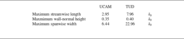

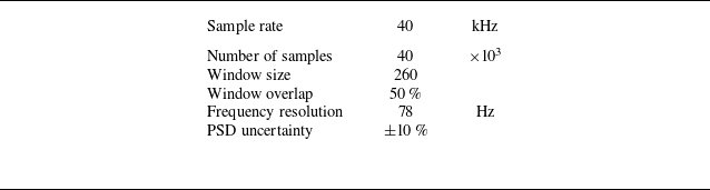
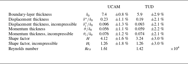


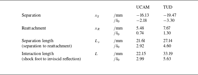


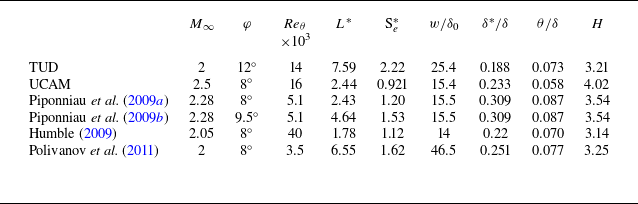


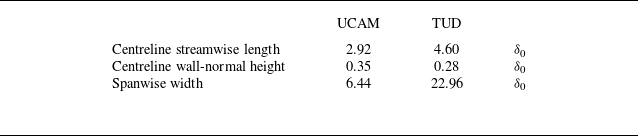


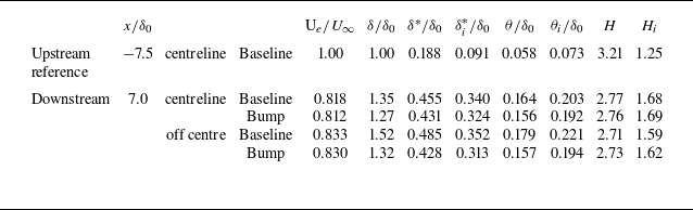


 Open access