1. Introduction

Sea-ice volume is an important parameter in identifying the impact of climate change at high latitudes, as has been shown for the Arctic (e.g. Reference Schweiger, Lindsay, Zhang, Steele, Stern and KwokSchweiger and others, 2011). More is known about Arctic than Antarctic sea-ice volume, as detailed below. A large number of submarine upward-looking sonar (ULS) observations have been carried out in the Arctic Ocean (e.g. Reference Rothrock and WensnahanRothrock and Wensnahan, 2007), but these are completely lacking in the Southern Ocean. Only data from moored ULS in the Weddell Sea are available (Reference Harms, Fahrbach and StrassHarms and others, 2001; Reference BehrendtBehrendt and others, 2011). In the Arctic, retrieval of sea-ice thickness using laser or radar altimetry has been more successful and is better validated (Reference Connor, Laxon, Ridout, Krabill and McAdooConnor and others, 2009, 2013; Reference Kwok, Cunningham, Zwally and YiKwok and others, 2009; Reference LaxonLaxon and others, 2013). For Antarctica, sea-ice thickness validation data sources are extremely sparse. Hence, validation of new approaches for satellite sea-ice thickness retrieval is limited to relatively few in situ observations (e.g. Reference Worby, Markus and SteelWorby and others, 2008; Reference Ozsoy-Cicek, Ackley, Xie, Yi and ZwallyOzsoy-Cicek and others, 2013) and to intercomparisons with alternative methods. Therefore careful uncertainty estimations should play an important role, which is the motivation for this study. This paper focuses on satellite laser altimetry, which has shown great potential for deriving Antarctic sea-ice thickness from measurements of the Geoscience Laser Altimeter System (GLAS) aboard the Ice, Cloud and land Elevation Satellite (ICESat) (e.g. Reference Zwally, Yi, Kwok and ZhaoZwally and others, 2008; Reference Markus, Massom, Worby, Lytle, Kurtz and MaksymMarkus and others, 2011; Reference XieXie and others, 2011, Reference Xie, Tekeli, Ackley and Yi2013; Reference YiYi and others, 2011; Reference Kurtz and MarkusKurtz and Markus, 2012).

The basis for sea-ice thickness retrieval from satellite laser altimetry data is the elevation of the topmost ice surface above the sea surface. A laser altimeter permits the elevation of the topmost sea ice or sea ice plus snow surface above the sea surface (the so-called sea ice + snow = total freeboard) to be obtained. Thereafter a buoyancy approach can be applied to convert total freeboard to sea-ice thickness provided that the densities of sea water, snow and sea ice as well as the snow depth are known (Reference Kwok, Zwally and YiKwok and others, 2004). To derive total freeboard, the instantaneous sea-surface height (SSH) is required. This time-varying height includes, among others, contributions from atmospheric loading, ocean surface undulations due to eddy currents, and ocean tides. The instantaneous SSH cannot be obtained from other data sources with the spatiotemporal resolution required for total freeboard retrieval. Numerical models used to compute the time-varying component of the SSH do not currently reveal satisfying results (e.g. Reference Price, Rack, Haas, Langhorne and MarshPrice and others, 2013). Therefore the SSH is approximated from altimeter measurements by finding open water and thin ice associated with new leads in the sea-ice cover.

Sea-ice thickness retrieved from ICESat is most sensitive to variations and uncertainties in the total freeboard, as shown by Reference Kwok and CunninghamKwok and Cunningham (2008) for the Arctic. Variation and uncertainty in snow depth is the second most important contribution to sea-ice thickness retrieval using laser altimetry (Reference GilesGiles and others, 2007; Reference Kwok and CunninghamKwok and Cunningham, 2008). Contributions from uncertainties in the densities of sea ice and snow are smaller, but together can exceed the contribution from snow depth uncertainty to sea-ice thickness uncertainty. The vertically and horizontally heterogeneous snow cover on Antarctic sea ice complicates the impact of the snow cover on sea-ice thickness retrieval using altimetry.

For the Arctic a number of detailed investigations have been carried out dealing with uncertainties involved in different approaches to retrieving total freeboard from ICESat data and finding an optimal approach to derive total freeboard (e.g. Reference Spreen, Kern, Stammer, Forsberg and HaarpaintnerSpreen and others, 2006; Reference GilesGiles and others, 2007; Reference Kwok, Cunningham, Zwally and YiKwok and others, 2007; Reference Farrell, Laxon, McAdoo, Yi and ZwallyFarrell and others, 2009; Reference KurtzKurtz and others, 2009). Reference Kwok, Cunningham, Zwally and YiKwok and others (2007) tested three approaches: approach A requires contemporary high-resolution satellite radar or clear-sky optical imagery to identify leads; approach B takes advantage of leads being associated with a low reflectivity measured by ICESat; and approach C takes into account the relation between local surface elevation and elevation standard deviation over a predefined ground segment of the ICESat ground track. For Antarctica, it seems impractical to use approach A because of the lack of sufficient contemporary satellite data. Approach B cannot be used because leads are often associated with both low and high reflectivities, so the reflectivity cannot be used as a reliable lead indicator. The concept of relating the local surface elevation to the standard deviation of the elevation introduced in approach C is the basis for the approach developed by Reference Markus, Massom, Worby, Lytle, Kurtz and MaksymMarkus and others (2011). This approach is based on observations of snow depth, total freeboard and sea-ice thickness in the East Antarctic but it uses the aforementioned concept only to constrain the number of potential elevations used to select SSH tie points, which is done in a similar way to the lowest-level elevation method (see next paragraph). The approach of Markus and others (2011) is used to obtain Antarctic sea-ice thickness from ICESat (Reference Kurtz and MarkusKurtz and Markus, 2012). Reference Kurtz and MarkusKurtz and Markus (2012) avoided the impact of a potentially biased snow depth product (e.g. due to widespread ice–snow interface flooding) by assuming zero sea-ice freeboard everywhere and thus taking ICESat total freeboard as a measure of snow depth. Reference XieXie and others (2011, Reference Xie, Tekeli, Ackley and Yi2013) developed an approach based on in situ measurements obtained in the Bellingshausen/Amundsen Seas. In contrast to Reference Markus, Massom, Worby, Lytle, Kurtz and MaksymMarkus and others (2011), the approach of Reference Xie, Tekeli, Ackley and YiXie and others (2013) is empirical and does not rely on the hydrostatic equilibrium. Reference Ozsoy-Cicek, Ackley, Xie, Yi and ZwallyOzsoy-Cicek and others (2013) investigated in situ measurements from expeditions into the Antarctic sea-ice cover during the past 20 years and suggest a set of empirical equations to convert total freeboard directly into sea-ice thickness. Both empirical approaches confirm that the assumption of a zero sea-ice freeboard can be reasonable for some regions. For both these approaches snow depth is not required, similar to Reference Kurtz and MarkusKurtz and Markus (2012). While it is an advantage not to depend on snow depth data, it is necessary to show the extent to which the assumption of zero sea-ice freeboard is valid and whether the empirical approaches can be applied universally.

In this paper we investigate the approach developed by Reference Zwally, Yi, Kwok and ZhaoZwally and others (2008) and refined by Reference YiYi and others (2011). They applied the so-called lowest-level elevation method. This method assumes that ICESat detects open water or thin ice present in leads as elevation minima in at least 2% of the elevation residua (Section 3) within a 50 km segment of one ICESat measurement profile. These minima serve as tie points to approximate the instantaneous SSH, which is used to compute total freeboard. Subsequently the hydrostatic equilibrium approach is used to convert total freeboard into sea-ice thickness. What is lacking for this approach is a quantification of the uncertainty of the total freeboard retrieval due to input parameters of the lowest-level elevation method. Improved knowledge of this uncertainty could provide a better measure of the per gridcell uncertainty of total freeboard and hence of sea-ice thickness computed from it. Such quantification becomes even more important once the approaches used to derive sea-ice thickness rely predominantly on total freeboard (e.g. Reference Markus, Massom, Worby, Lytle, Kurtz and MaksymMarkus and others, 2011; Reference Ozsoy-Cicek, Ackley, Xie, Yi and ZwallyOzsoy-Cicek and others, 2013; Reference Xie, Tekeli, Ackley and YiXie and others, 2013).

This paper discusses the results of a sensitivity analysis varying several input parameters for the approach used by Reference Zwally, Yi, Kwok and ZhaoZwally and others (2008) and Reference YiYi and others (2011) (e.g. the aforementioned 2%, which is an empirically chosen number). The present paper gives theoretical ice thickness uncertainty estimates as a function of snow depth. Furthermore, an estimate of the actual sea-ice thickness uncertainty is given for the Weddell Sea based on ICESat total freeboard and snow depth from satellite microwave radiometry applying Gaussian error propagation to the approach used by Reference YiYi and others (2011). The obtained total freeboard and sea-ice thickness distribution is also compared with the results of Reference Kurtz and MarkusKurtz and Markus (2012).

2. Data

Here we use GLAS/ICESat L2 sea-ice altimetry data (GLA13) of release 33 (Reference ZwallyZwally and others, 2011). The data are downloaded for ICESat measurement periods 2B to 3G (FM04 to ON06 in Table 1) from the US National Snow and Ice Data Center (NSIDC) (http://nsidc.org/data/gla13.html). The data are pre-processed with software provided by the NSIDC (http://nsidc.org/data/icesat/tools.html); here the Interactive Data Language (IDL) readers are used. As is recommended by Reference ZwallyZwally and others (2011), the following corrections and flags are applied to the surface elevations: i_reflctUC, i_reflCor_atm, i_gval_rcv, i_Surface_pres, i_satElevCorr, i_satCorrFlg. Resulting surface elevations are given relative to the EGM08 geoid (Reference Pavlis, Holmes, Kenyon and FactorPavlis and others, 2012) provided together with the ICESat data (i_gdHt). We did not carry out the G-C offset correction (Reference Borsa, Moholdt, Fricker and BruntBorsa and others, 2014): firstly, the present paper deals with a sensitivity study rather than an attempt to provide the best sea-ice thickness computed from ICESat data; and secondly, the two approaches with which we compare our results also did not include the G-C offset correction.

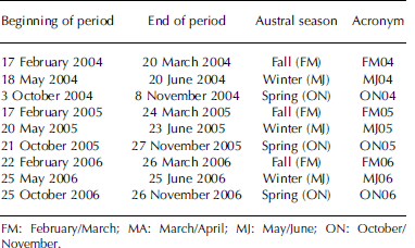
Table 1. ICESat periods used in the present study with the respective austral season and acronym

Freeboard is computed only for ice-covered areas. We used sea-ice concentrations calculated with the ARTIST (Arctic Radiation and Turbulence Interaction STudy) Sea Ice (ASI) concentration algorithm (Reference KaleschkeKaleschke and others, 2001; Reference SpreenSpreen and others, 2008) applied to 85 GHz Special Sensor Microwave/Imager (SSM/I) observations. ASI sea-ice concentrations are taken from the Integrated Climate Data Center (ICDC) (http://icdc.zmaw.de/seaiceconcentration_asi_ssmi.html_ ssmi.html) as 5day median-filtered gridded product with daily temporal and 12.5 km grid resolution. For higher sea-ice concentration in the range used here, uncertainty estimates are of the order of 5% (Reference SpreenSpreen and others, 2008). Only gridcells with a sea-ice concentration higher than 60% are used unless stated otherwise.

Conversion of freeboard into ice thickness using the approach of Reference YiYi and others (2011) requires snow depth data. We used the snow depth on sea ice from Advanced Microwave Scanning Radiometer for Earth Observing System (AMSR-E) satellite observations, as provided daily by the NSIDC as a 5 day running mean at a grid resolution of 12.5 km (Reference Cavalieri, Markus and ComisoCavalieri and others, 2004). This level 3 product (AE_SI12) is based on the modified snow depth retrieval algorithm of Reference Markus and CavalieriMarkus and Cavalieri (1998) (Reference Comiso, Cavalieri and MarkusComiso and others, 2003). AMSR-E snow depth was found to agree to within ∼0.05 m with in situ snow depth measurements and within ∼0.1 m with visual ship-based snow depth observations over level undeformed sea ice (Reference Worby, Markus and SteelWorby and others, 2008). Reference StroeveStroeve and others (2006) suggested that AMSR-E underestimates snow depth, on the basis of a model-assisted intercomparison of in situ snow depth and airborne microwave radiometry at AMSR-E frequencies. This was later confirmed and quantified: AMSR-E underestimates snow depth over rough deformed sea ice by a factor of 2 or more (Reference Worby, Markus and SteelWorby and others, 2008; Kern and others, 2011; Reference Ozsoy-Cicek, Kern, Ackley, Xie and TekeliOzsoy-Cicek and others, 2011). Melting and refreezing events, snow wetness and variable snow grain size can cause biases in the retrieved snow depth (Reference Markus and CavalieriMarkus and Cavalieri, 1998).

We use the dataset of Antarctic gridded total freeboard and sea-ice thickness available from the Cryosphere Science Research Portal at NASA (http://seaice.gsfc.nasa.gov/csb/index.php?section=272) (see also Reference Markus, Massom, Worby, Lytle, Kurtz and MaksymMarkus and others, 2011; Reference Kurtz and MarkusKurtz and Markus, 2012).

All data used in the present paper are gridded onto the polar stereographic NSIDC grid for the Southern Hemisphere (https://nsidc.org/data/polar_stereo/ps_grids.html) with a grid resolution of 25 km using nearest-neighbor interpolation.

3. Methods

We compute total freeboard from ICESat surface elevation observations (Section 2) using the approach of Reference YiYi and others (2011) and Reference Zwally, Yi, Kwok and ZhaoZwally and others (2008) for the Weddell Sea region west of 20° E. For a detailed description of the approach see Reference YiYi and others (2011) and Reference Zwally, Yi, Kwok and ZhaoZwally and others (2008); only key aspects are given here. First, elevations ˃4 m above the geoid are removed to discard icebergs (Reference Zwally, Yi, Kwok and ZhaoZwally and others, 2008). Secondly, residual elevation profiles are computed by subtracting an along-track averaged elevation profile from the original elevation profile. The result is a high-pass-filtered residual elevation containing only small spatial-scale variations in surface elevation of up to tens of centimeters. The width of the window used for averaging is hereafter referred to as high-pass filter (HPF) width and is one of the parameters varied in our sensitivity study (see below).

For the approximation of SSH from surface elevation residuals we use the so-called lowest-level elevation method (Reference Zwally, Yi, Kwok and ZhaoZwally and others, 2008). A window of length X, hereafter the ground-track segment (GTS), is moved along the elevation profile. Within the segment, elevations are sorted in ascending order and the lowest percentage (P) elevations are identified. These elevation minima are assumed to be caused by new leads with open water or very thin ice and are used as tie points to approximate SSH, which is subsequently subtracted from the elevations to obtain total freeboard.

In accordance with Reference Zwally, Yi, Kwok and ZhaoZwally and others (2008) we set GTS length to 50 km and term this the ‘master setting’. As in Reference YiYi and others (2011) the GTS is moved along track footprint-by-footprint, i.e. by a distance of 172 m. For each GTS, the lowest-level elevation method is applied. Note that we also use the same reflectivity and gain thresholds as used by Reference YiYi and others (2011). For the lowest-level percentage (P) we used 2% as the ‘master setting’, identical to Reference YiYi and others (2011). The only difference between our master setting and that of Reference YiYi and others (2011) is the different HPF width: we use 50 km, while Reference YiYi and others (2011) used 20 km. Figure 1 shows how a spatially varying freeboard is approximated much better when using a combination of GTS and HPF where GTS length is smaller than or equal to HPF width. In Figure 1a the red line approximates the artificial freeboard profile much better than the blue line; the red line is for HPF = GTS = 25 km, while the blue line is for HPF = 25km but GTS = 100 km. Therefore we choose HPF = GTS = 50 km in our master setting. We note that HPF should never be smaller than GTS, to avoid the incorrect freeboard artifacts illustrated in Figure 1 (blue lines). Therefore, in the entire sensitivity study we only allow combinations of HPF ˃ GTS.

Fig. 1. Negative impact of using a GTS length larger (blue) than the HPF compared with GTS = HPF (red) for an artificial freeboard profile (a; black line). The black line in (b) shows the profile of the high-pass-filtered elevation (HPF =25km) of the artificial freeboard shown in (a). Red and blue lines in (b) denote the SSH approximation obtained using a GTS of 25km (red) and 100 km (blue). The red and blue lines in (a) denote the approximated freeboard that is obtained from (b) for the above-mentioned GTS values.

In our sensitivity study we vary HPF width and GTS length. We choose values of 100, 50, 37.5, 25 and 12.5 km for both HPF width and GTS length, always with HPF˃ GTS. We also investigate how total freeboard retrieval is impacted by using no HPF. In addition we vary P between 1 % and 5%. This parameter defines the percentage of elevation minima assumed to be leads. If the actual number of leads within a GTS yields a larger percentage P than chosen, the SSH approximation is acceptable because the identified elevation minima most likely all correspond to leads with open water or very thin ice. However, if the actual number of leads within a GTS yields a lower percentage P than chosen, SSH could be biased high and thus total freeboard biased low. This is because in this case elevation minima are used as SSH tie points, which are not actually associated with new leads with open water or thin ice but originate from older leads with thicker sea ice. Another effect of the choice of P is illustrated in Figure 2a. If there is a sharp gradient or step in the elevation (e.g. due to a change in ice type) the choice of a low percentage P could cause SSH to be biased low and thus total freeboard to be biased high in the vicinity of that gradient or step in elevation. A high percentage P would be less affected by this. Consequently, we expect that a higher percentage P results in a smaller total freeboard. Within a GTS there have to be sufficient valid ICESat measurements that at least three elevation minima can be selected; otherwise the freeboard for this particular GTS is discarded. Depending on the choice of GTS length and P, there could be several GTS discarded (see Fig. 2b).

Fig. 2. Impact of using a large (P= 5%) versus a small (P= 1%) percentage for the lowest-level elevation method (a) and the number of minima potentially found for two different GTS lengths (b) illustrated with artificial high-pass-filtered elevation profile.

For the sea-ice thickness retrieval we use the same densities as Reference YiYi and others (2011). Following Reference Zwally, Yi, Kwok and ZhaoZwally and others (2008) we discard total freeboard values exceeding

1 m. The snow depth is taken from the AMSR-E snow depth product, similar to Reference YiYi and others (2011). Note that, in contrast to the Arctic, for Antarctica sea-ice freeboard can be close to zero or even negative (e.g. Reference MassomMassom and others, 2001). AMSR-E snow depth should be less than, or at maximum equal to, total freeboard. However, as indicated by Reference Zwally, Yi, Kwok and ZhaoZwally and others (2008) and Reference YiYi and others (2011) and confirmed in the present paper, this is not always the case. Reference YiYi and others (2011) reported that during austral summer AMSR-E snow depth can exceed total freeboard from ICESat in up to 4 0% of the sea-ice area investigated. Therefore, Reference YiYi and others (2011) discriminated between these cases and used Eqn (1) for cases with a positive difference between freeboard and AMSR-E snow depth and Eqn (2) for the other cases in which they assumed that snow depth equals total freeboard:

(1)

(2)

We follow Reference YiYi and others (2011) to compute sea-ice thickness from mean ICESat freeboard and mean AMSR-E snow depth. Here ‘mean’ refers to the mean value obtained from both parameters for the entire corresponding ICESat measurement period (Table 1 ) within one 25 km gridcell. Note that, even though ICESat measurement periods have durations of ∼33-35 days, the number of days with ICESat measurements that contribute to mean freeboard is on average 1-2 days at a grid resolution of 25 km (as also used in Reference YiYi and others, 2011). This is exemplified in Figure 3 for period 2C. Only very few gridcells contain data of ˃2 days. By using Gaussian error propagation (e.g. Reference Spreen, Kern, Stammer, Forsberg and HaarpaintnerSpreen and others, 2006; Reference Farrell, Laxon, McAdoo, Yi and ZwallyFarrell and others, 2009; Reference Kwok, Cunningham, Wensnahan, Rigor, Zwally and YiKwok and others, 2009) we carry out an uncertainty estimation of the sea-ice thickness using

(3)

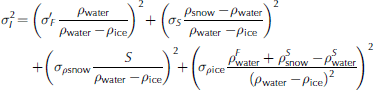
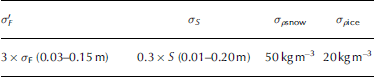
Values used for the uncertainties of freeboard, σ' _F, snow depth, σ_S, and the densities of sea ice, σ_{ρ ice} , and snow, σ_ρsnow, are given in Table 2. Density uncertainties are based on Maksym and Reference Markus and MarkusMarkus (2008) and Reference MassomMassom and others (2001). We neglect uncertainties due to sea-water density variations as suggested by Reference Kwok and CunninghamKwok and Cunningham (2008). The AMSR-E snow depth product does not provide uncertainty information. Uncertainties given in Reference Markus and CavalieriMarkus and Cavalieri (1998) are contradicted by the findings of Reference Worby, Markus and SteelWorby and others (2008) and other studies (Section 1). Hence we suggest following Reference Spreen, Kern, Stammer, Forsberg and HaarpaintnerSpreen and others (2006), and use a snow-depth-dependent uncertainty of 30% of the AMSR-E snow depth. Biases between AMSR-E snow depth and in situ measurements are higher on a daily basis over deformed sea ice, but in the present paper we use snow depths averaged over ∼ 1 month. In this context, we propose that using 30% of the snow depth is a conservative uncertainty estimate. For the theoretical sea-ice thickness uncertainty calculations we exemplarily assume an uncertainty in total freeboard of 0.05 m. Our choice of uncertainties in total freeboard used for our sea-ice thickness retrieval is discussed further in Section 5.

Fig. 3. Number of days within ICESat measurement period MJ04 (Table 1) for which freeboard data are obtained at a grid resolution of 25 km.

Table 2. Values used for the uncertainty computation with Eqn (3) and in our sea-ice thickness retrieval. Values used for ρ_snow, ρ _ice and ρ_water are 300.0, 915.1 and 1023.9 kg m^–3 respectively, as used in Reference YiYi and others (2011). Values given in parentheses in the first two columns denote the typical value range

4. Results

4.1 Theoretical sea-ice thickness error estimation

Theoretical estimates of the absolute and relative error in sea-ice thickness are computed with Eqn (3) and shown in Figure 4 as a function of total freeboard F for different snow depths S. Here a total freeboard uncertainty of 0.05 m is the example used. The error estimates are calculated from Gaussian error propagation of Eqn (1), i.e. Eqn (3), even for cases with F≤S Eqn (2)) allowing uncertainties in snow depth for the full freeboard range. If uncertainties in snow are neglected for F≤S (Eqn (2)), much smaller error estimates are obtained for these freeboard ranges.

Fig. 4. Absolute (a) and relative (b) error estimate in sea-ice thickness as a function of total freeboard for different snow depths as computed using Eqn (3).

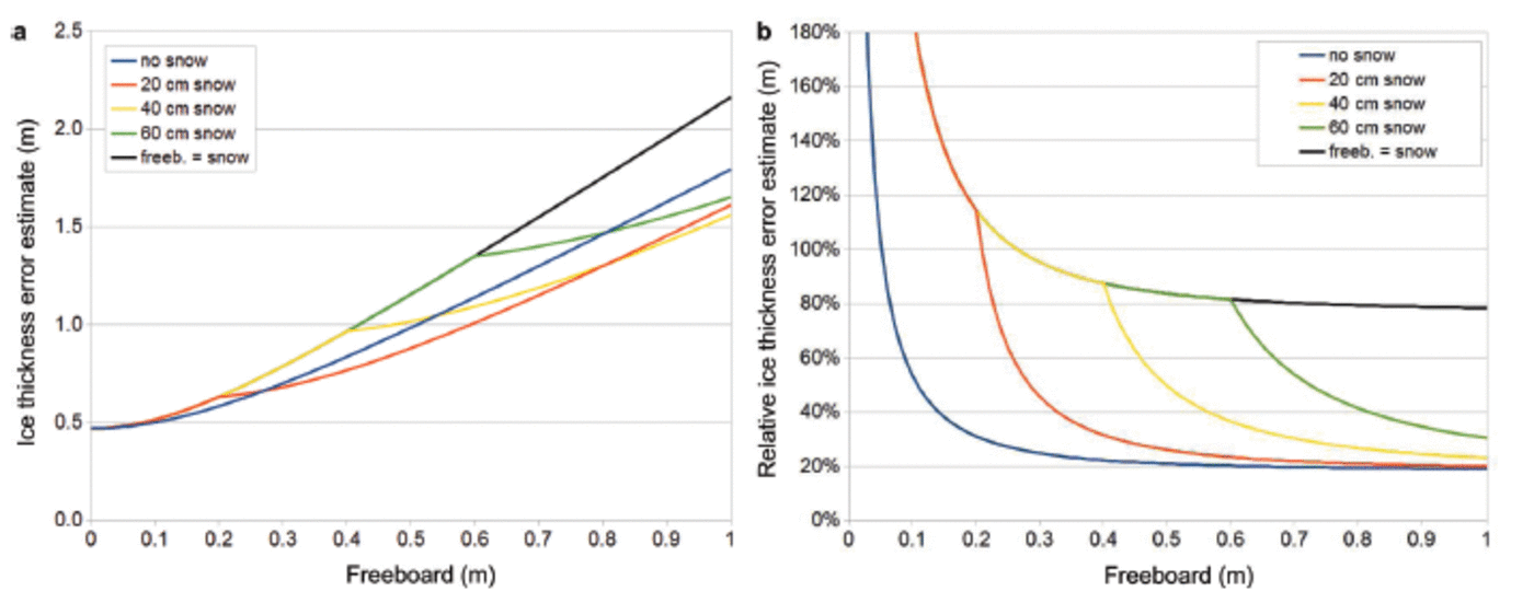
For all snow cases the absolute thickness error increases with total freeboard F. When F≥S, the increase rate is reduced. Therefore the no-snow case (black) intersects the snow cases (Fig. 4). For the relative error, which is absolute error divided by ice thickness (Fig. 4b), this behavior changes. It is possible to distinguish between three cases. Case 1 is bare ice (no snow) where the relative ice thickness error decreases rapidly from ∼100% at a freeboard of 0.05 m to 50% at 0.10 m freeboard and ∼30% at a freeboard of 0.20 m. Case 2 is when freeboard equals snow depth. In this case the relative ice thickness error is much higher than for bare ice and does not drop below 80% for the freeboard range shown in Figure 4, while the relative uncertainty for bare ice converges towards 20% at a freeboard of 0.50 m. Case 3 includes the intermediate cases, which comprise given snow depths that are (theoretically) higher than total freeboard until it exceeds the snow depth (red line in Fig. 4). Hence the curve of the relative ice thickness error first follows the curve for case 2. Once total freeboard equals snow depth the relative ice thickness error decreases rapidly and converges towards the curve for case 1, reaching, for example, 30% relative error at a freeboard of 40%, which equals 0.20 m snow on top of 0.20 m ice elevation above the waterline. The numbers given are specific to the error assumptions made (see above). For example, if the error estimate of snow depth S is changed to 20% (not shown) instead of 30%, the case 2 line (F = S; black) would converge towards 57% and not 80%; however, the general pattern would remain the same.

4.2. Freeboard

How does the choice of HPF width, GTS length and lowest-level elevation method percentage (P) influence total freeboard retrieval along single ICESat elevation profiles? Figure 5a shows the difference between gridded freeboard along one profile derived with the master setting minus the freeboard derived with same setting but no high-pass filtering for different GTS lengths. The location of the profile is indicated in Figure 5c. Figure 5a reveals that for the profile chosen, independent of GTS length, total freeboard is underestimated relative to the master setting over about the first ten gridcells, which corresponds to a distance of at least 250 km.

Fig. 5. Impact of choice of freeboard retrieval parameter on two selected ICESat tracks delineated in (c) and (d). (a) Freeboard difference of master setting minus alternative setting for different GTS lengths using no HPF. (b) Freeboard difference master setting minus alternative setting for different GTS lengths for HPF = 50 km. (e) Freeboard for different GTS lengths, HPF = 50 km, for lowest-level elevation method percentage P = 5% (lines) compared with master setting (uses P = 2%, diamonds). (f) Freeboard for different HPF = GTS combinations (lines) compared with the master setting (diamonds). Date format is year.month.day.

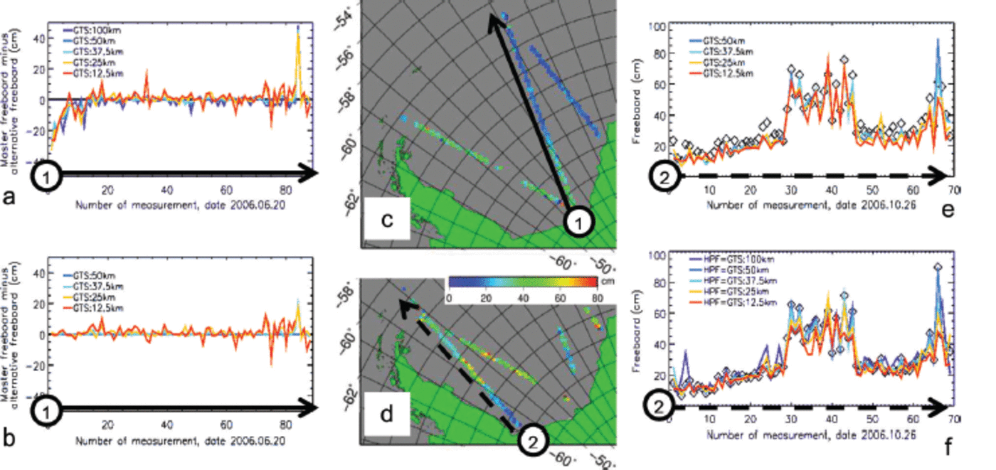
In Figure 5b GTS length is varied for the same profile while all other parameters are kept constant. Absolute differences remain local and ˂ 0.10m for the majority of the profile, independent of GTS length, except towards the northern end where the ice cover is less homogeneous and the differences increase.

Using a larger percentage P is expected to cause a decrease in obtained total freeboard as long as enough leads are present; otherwise total freeboard is likely to be overestimated in comparison to using a lower percentage P. Figure 5e gives an example of the first case: freeboard derived for the profile shown in Figure 5d with P = 5% (colored lines) is smaller than freeboard derived for this profile with the master setting P = 2% (diamonds); the difference is between 0.05 and 0.10m. This seems to be more or less independent of GTS length. However, the difference is not as large for every gridcell. There are also gridcells (39 and 66) where the sign of the difference reverses and the freeboard obtained for P = 5% is larger than that obtained for P= 2%.

Finally, in Figure 5f we demonstrate for the profile shown in Figure 5d whether a change in HPF and GTS, here setting HPF= GTS, changes freeboard in comparison to the master setting. Total freeboard obtained for HPF =GTS = 12.5 km (red line) tends to give the lowest values, while total freeboard obtained for HPF =GTS= 100 km (dark blue line) tends to give the highest values. Use of a longer segment potentially causes overestimation of freeboard compared with use of a shorter segment, particularly over areas with spatially heterogeneous freeboard distributions. All five HPF/GTS combinations allow identification of the area of larger freeboard between about 71° S and 68° S, similar to the master setting (HPF =GTS= 50km).

Figure 6 illustrates that the results shown in Figure 5 have implications for the overall mean freeboard distribution obtained from all gridded ICESat overpasses within an ICESat measurement period. Note that the filters used in the data pre-processing, such as the gain filter and the filter that removes too low and too high reflectance values, substantially reduce the number of valid ICESat data. These filters are the main reason for the large number of data gaps, denoted as white areas in the maps (Fig. 6–8). Figure 6a expands on Figure 5a and shows for period MJ06 (Table 1) an area of negative freeboard differences stretching along the Antarctic coast when no HPF is used. Differences exceed 0.10 m, illustrating that omission of the high-pass filtering can lead to overestimation of total freeboard compared with the master setting. Most of the remaining area reveals differences close to zero. Along the ice edge, differences tend to be larger; however, both positive and negative differences are observed here. The histogram in Figure 6b shows an asymmetric distribution, with mode and median being only slightly negative: –0.005 and –0.021 m, respectively. The tail towards negative differences is much more pronounced than that towards positive differences. Table 3 lists modal and mean total freeboard for all periods used (Table 1) for this setting in its last row, together with the average difference to the master setting (first row) in the last column. Omission of the high-pass filtering causes higher freeboard values along the coast but has little influence on the overall modal and mean total freeboard.

Figure 6c expands on Figure 5e and shows for period MJ06 (Table 1 ) that using P= 5% instead of P= 2% causes widespread overestimation of total freeboard compared with the master setting without any regional pattern like that observed in Figure 6a. The histogram (Fig. 6d) is also asymmetric and exhibits a clear positive mode at 0.025 m and a mean of 0.036 m. Positive differences dominate and exceed 0.10m. Table 3 summarizes modal and mean total freeboard for this alternative setting (percentage P = 5% and GTS = 50 km and 25 km) in the second and fourth rows, respectively. The mean difference from the master setting for the nine periods shown is given in the last column and takes a value 0.06 m for modal total freeboard and between 0.04 and 0.06 m for mean total freeboard. Using P = 5% results in an overall decrease of the gridcell freeboard standard deviation of 0.001-0.002 m, i.e. ∼10%.

Fig. 6. Difference of total freeboard obtained for ICESat measurement period 3F (Table 1 ) with the master setting minus the alternative setting using (a) no HPF and (c) a percentage P= 5%. (b, d) Histograms associated with (a) and (c). (e) Difference in total freeboard using HPF=100 km, GTS=25km minus freeboard using HPF=GTS=100 km, together with the corresponding histogram (f). White areas show the ICESat measurement period mean sea-ice extent using a 30% sea-ice concentration threshold.

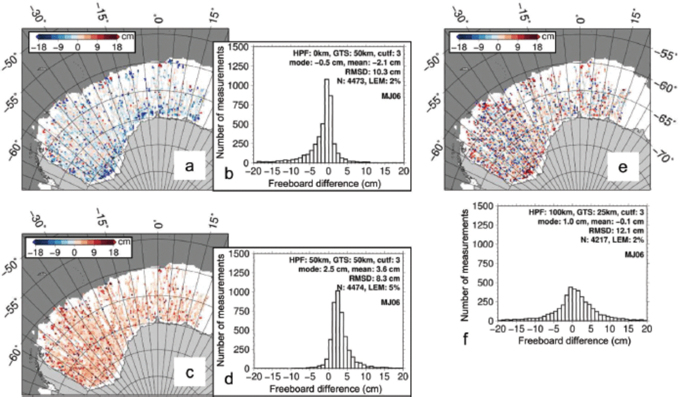
Table 3. Overview of modal freeboard/mean freeboard for ICESat periods FM04–ON06 (Table 1 ). First row: master setting; second row: master setting but percentage P= 5%; third row: master setting but GTS=25km; fourth row: master setting but percentage P=5% and GTS =25 km; fifth row: master setting but without high-pass filtering. The last column denotes the difference from the master setting (first row). Highlighted in bold are differences from the master setting exceeding 0.05 m

Table 4. Mean and modal total freeboard (m) for the Weddell Sea region from Reference YiYi and others (2011), the present study using the ‘master setting’ (see text and Table 2) and from Reference Kurtz and MarkusKurtz and Markus (2012). Note that model total freeboard is not available for Reference YiYi and others (2011)

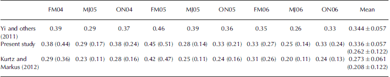
Figure 6e shows that using GTS = 25 km instead of 100 km causes both positive and negative differences in total freeboard; absolute values can exceed 0.10 m. Regional patterns are difficult to identify; large negative difference, i.e. GTS = 100 km, provides larger freeboard than GTS = 25km, and seems to be present more in the central Weddell Sea, while large positive differences occur in some coastal areas and along the ice edge. The overall mean difference is zero (Fig. 6f). This is also demonstrated in Table 3 where the difference in modal and mean total freeboard between the third (GTS = 25km) and first rows (GTS = 50 km) averaged over nine ICESat periods is zero.

5. Discussion

5.1 Freeboard and freeboard uncertainty

We have investigated the sensitivity of total freeboard retrieval, applying the lowest-level elevation method to ICESat surface elevation measurements with respect to three main input parameters. These are HPF width, and GTS length and percentage (P) used to define tie points for SSH approximation.

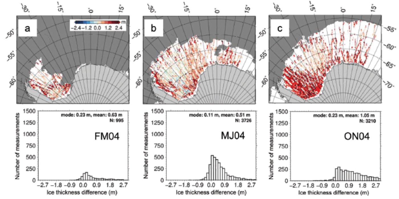
Figure 7 shows the total freeboard distribution obtained with the master setting for ICESat periods FM04, MJ04 and ON04 (Table 1); maps are shown in Figure 7a–c and corresponding histograms in Figure 7d–f. Freeboard distribution and the shape of the histograms compare well with the findings of Reference YiYi and others (2011). Mean total freeboard values of all periods used (Table 1) agree to within 0.03 m with those of Reference YiYi and others (2011). The averages over all nine periods are 0.336m (present study) and 0.344m (Reference YiYi and others, 2011); the corresponding standard deviations are the same (Table 4). Note that, in contrast to Reference YiYi and others (2011), we did not interpolate gaps between tracks. Figure 7g–i show the mean ICESat sensor single-shot precision as one component of the retrieval uncertainty. It is computed as 0.138 m divided by the square root of the number of single ICESat measurements falling into one 25 km gridcell, and hence strongly depends on the number of valid ICESat elevation measurements (cf. Fig. 3). This component of the uncertainty varies between 0.01 and 0.02 m, its mode is close to 0.01 m and values greater than 0.04 m are virtually absent. We note that the standard deviation of the mean gridded freeboard, i.e. the variation of freeboard values for each gridcell (not shown), is ∼0.5F.

Fig. 7. (a–c) Total freeboard obtained with the master setting for the three ICESat measurement periods in 2004: (a) FM04, (b) MJ04 and (c) ON04 (Table 1 ). (d–f) Histograms for the images in (a–c). (g–i) Mean ICESat single-laser-shot precision per gridcell for the same periods as given in (a–f). White areas show the ICESat measurement period mean sea-ice extent using a 60% sea-ice concentration threshold.

Our sensitivity study reveals that the choice of input parameters, such as P and GTS length, as well as application of a HPF that has an appropriate width, i.e. larger than or equal to GTS length, has an impact on modal and mean total freeboard, on its variability and on its spatial distribution in the Weddell Sea. The differences observed in this sensitivity study could therefore be used to support error estimation applying the lowest-level elevation method to ICESat data for total freeboard retrieval. The observed mean differences between the different settings can amount to 0.04 m (Table 3 last column), while locally these can exceed 0.10 m. The two largest contributions are caused by application of a HPF prior to SSH approximation and by the percentage (P) used to define how many new leads can be found in an ICESat elevation profile of length GTS. The difference between application and non-application of a HPF causes an overall mean bias in total freeboard of only ∼0.02 m. However, extended regions, like that shown in Figure 6a, can exhibit biases of 0.05 m or more.

How can we incorporate the observed uncertainties in the SSH approximation, and hence in total freeboard retrieval using the lowest-level elevation method, into sea-ice thickness retrieval to provide a physically meaningful per gridcell uncertainty estimate for sea-ice thickness? It seems obvious that for total freeboard a true measure of the uncertainty would require more in situ freeboard data for comparison or a more sophisticated approach to evaluate the SSH quality (e.g. with synthetic aperture radar (SAR) data as reported by Reference Kwok, Cunningham, Zwally and YiKwok and others (2007) for Arctic sea ice). A similar methodology could be developed for Antarctic sea ice provided that the approaches used by Reference Kwok, Cunningham, Zwally and YiKwok and others (2007) can be tested here. This is beyond the scope of the present paper. The precision of ICESat elevation measurement is of the order of 0.02 m (Reference Kwok, Zwally and YiKwok and others, 2004) and the elevation accuracy is ∼0.03-0.04 m (Reference Connor, Farrell, McAdoo, Krabill and ManizadeConnor and others, 2013). Quantification of the latter was possible because ICESat elevation measurements could be combined with contemporary airborne laser altimeter measurements. Contemporary ICESat and airborne laser altimeter data do not exist for the Weddell Sea, the focus of the present paper.

In principle, we could simply take a constant uncertainty value by combining the aforementioned two numbers (0.02 m and 0.03-0.04 m), resulting in an uncertainty value of ∼0.03 m, but this would not reflect the large spatial variability of valid ICESat measurements per gridcell. Furthermore, the results of Reference Connor, Farrell, McAdoo, Krabill and ManizadeConnor and others (2013) might not be valid for the Weddell Sea. From our computations we see that the single-laser-shot precision of 0.138 m translates into a per gridcell contribution to total freeboard uncertainty of ∼-0.01-0.02 m, which varies with the number of valid ICESat measurements (Fig. 7g-i). Our sensitivity study revealed that total freeboard as obtained with the lowest-level elevation method can change as a function of input parameters to this method by between 0.05 and 0.10 m over large areas. Therefore, to obtain a more reasonable estimate of total freeboard uncertainty for our error propagation with Eqn (3) than the standard deviation of the mean freeboard suggested by Reference YiYi and others (2011), and to comply with the aforementioned studies, we apply an empirical factor of 3 to the calculated mean single-laser-shot precision and use the result as freeboard error estimate a' _F in Eqn (3). This results in a gridded total freeboard uncertainty of at least 0.03 m for the entire region of interest and the distribution of which takes into account the number of valid measurements per gridcell. The choice of a value of 3 for this empirical factor is still arbitrary; the factor might need to be even higher. However, without further evaluation data to quantify the difference between measured and actual surface elevation there is limited added value in further refining such an empirical factor. It is meant to allow a per gridcell estimate of total freeboard uncertainty that takes into account the varying number of valid ICESat elevation measurements and which allows us to give a per gridcell estimate of sea-ice thickness uncertainty. It is obtained with Eqn (3), and the values listed in Table 2 are shown in Figure 8.

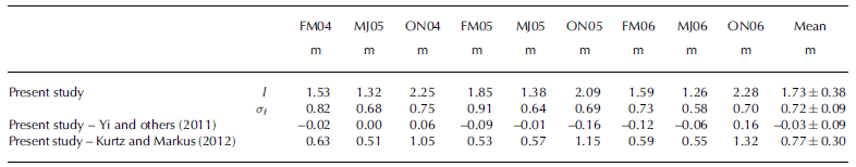
Table 5. Sea-ice thickness (I) and its uncertainty 0 _I for ICESat measurement periods 2B-3G (Table 1 ) as obtained in the present study. Also shown is the difference between ice thickness from the present study and that from Reference YiYi and others (2011) and Reference Kurtz and MarkusKurtz and Markus (2012)

Fig. 8. (a–f) Sea-ice thickness for ICESat measurement periods (Table 1 ; Fig. 6) in 2004 as maps (a–c) and histograms (d–f). (g–l) Corresponding retrieval uncertainty maps (g–i) and histograms (j–l). White areas show the ICESat measurement period mean sea-ice extent using a 60% sea-ice concentration threshold. All calculations were conducted using the master setting for total freeboard retrieval (see text and Table 2).

The choice of the empirically set percentage P is critical, as noted by Reference Zwally, Yi, Kwok and ZhaoZwally and others (2008) and Reference Price, Rack, Haas, Langhorne and MarshPrice and others (2013). In contrast to the Arctic, where during winter the open-water fraction due to leads may not exceed 0.5% (Reference KwokKwok, 2002), in Antarctica the open-water fraction is expected to be substantially higher and more variable because sea ice is not bounded by land. Therefore choosing P = 2% can only be a compromise. Reference Price, Rack, Haas, Langhorne and MarshPrice and others (2013) chose P = 5% for their local study in McMurdo Sound, Ross Sea. Figure 6c demonstrates that total freeboard would be smaller by 0.05-0.10 m over large areas of the Weddell Sea region if P = 5% was used instead of P = 2%. In order to choose an optimal percentage (P) additional contemporary data could be used. However, this is difficult in the Southern Ocean for the ICESat measurement periods because of limited spatial coverage and cloud and daylight effects for high-resolution radar and optical imagery. Sea-ice concentration data from satellite microwave radiometry available for the ICESat period are not accurate enough to identify sea-ice concentration changes of a few percent at high ice concentrations (Reference Andersen, Tonboe, Kaleschke, Heygster and PedersenAndersen and others, 2007). Further, lead location or concentration products that could help (Reference Röhrs and KaleschkeRöhrs and Kaleschke, 2012; Reference Willmes and HeinemannWillmes and Heinemann, 2015) are not available for the Southern Ocean.

One aspect that has been mentioned only briefly is the minimum number of minima required for SSH approximation (in our case three), which has an influence on total freeboard variability and more so on the number of usable freeboard data (Fig. 2b). The optimal choice among all these parameters depends on the ice conditions (e.g. ice type variations, surface roughness and number of leads), which are not known in advance. Therefore, any setting of these parameters can only be a compromise and is likely to represent certain sea-ice conditions better than others.

Finally, we note that the so-called G-C offset correction (Reference Borsa, Moholdt, Fricker and BruntBorsa and others, 2014), which has been omitted in this study to enable comparison of the results with those of Reference YiYi and others (2011) and Reference Kurtz and MarkusKurtz and Markus (2012), is another source of uncertainty, which should be corrected for and which has not been taken into account in our considerations.

5.2. Sea-ice thickness and its uncertainty

We compute sea-ice thickness for the Weddell Sea region from the obtained total freeboard as described in Section 3 and show the results in Figure 8a-f. The mean values are summarized in Table 5 together with the differences: mean sea-ice thickness using our approach minus Reference YiYi and others (2011), and our approach minus Reference Kurtz and MarkusKurtz and Markus (2012). Figure 8g-l show estimates of sea-ice thickness uncertainty. For austral fall, period FM04, modal sea-ice thickness uncertainty is 0.85 m; this corresponds to a relative error in modal sea-ice thickness of ∼80% (Fig. 8d). Mean sea-ice thickness uncertainty is 0.82 m; this corresponds to a relative error in mean sea-ice thickness of ∼55%. Modal and mean sea-ice thickness uncertainties are smaller for the austral winter (MJ04) and spring (ON04) periods: 0.45 m (mode) and 0.68 m (mean) in winter and 0.58 m (mode) and 0.75 m (mean) in spring. Relative uncertainty in modal sea-ice thickness is thus ∼60% for winter and spring. Relative uncertainty in mean sea-ice thickness is ∼50% in winter and 35% in spring, when the largest mean ice thickness is found (Fig. 8f). Mean sea-ice thickness uncertainty over all periods is 0.72 ± 0.09 m (Table 5), which is close to 40% of the mean sea-ice thickness value of 1.73 ± 0.38 m.

Differences in mean sea-ice thickness between the present study and Reference YiYi and others (2011) are largest for periods ON05 and ON06 (0.16 m; Table 5). The average (over all periods) difference in sea-ice thickness is only 0.02 m (Table 5). The standard deviation of the average mean ice thickness is 0.38 m and 0.36 m in this study and Reference YiYi and others (2011), respectively. In contrast, the difference between this study and Reference Kurtz and MarkusKurtz and Markus (2012) is 0.77 ± 0.30 m (Table 5). Differences range between 0.51 m (period MJ04) and 1.32 m (period ON06). Sea-ice thickness values obtained in the present study and hence also by Reference YiYi and others (2011) are substantially larger than those obtained by Reference Kurtz and MarkusKurtz and Markus (2012).

Figure 9 shows the difference between sea-ice thickness in the present study minus sea-ice thickness from Reference Kurtz and MarkusKurtz and Markus (2012) for the three ICESat periods in 2004. In most areas, sea-ice thickness from the present study is larger than that from Reference Kurtz and MarkusKurtz and Markus (2012). The area where this occurs tends to increase with season and is largest for period ON04 (Fig. 9c). The largest differences occur close to the coast and in the southern and western Weddell Sea. Negative differences (blue) are virtually absent. Areas with zero difference, which appear light green in Figure 9, indicate regions where both approaches are based on the same assumption: zero sea-ice freeboard and hence snow depth equal to total freeboard measured by ICESat (i.e. the region where Eqn (2) is applied). Provided that both total freeboard and snow depth are correct, these could be regions where flooding takes place. This would require a more in-depth investigation, which is beyond the scope of the present paper. Presumably the light blue and light red areas (±0.15 m) also belong to the region where, when taking the sea-ice thickness retrieval uncertainties into account, the present study (and hence Reference YiYi and others, 2011) and Reference Kurtz and MarkusKurtz and Markus (2012) provide similar values. However, over a large area the differences are substantially larger than ±0.15 m, suggesting further investigation of the validity of both approaches.

Fig. 9. Sea-ice thickness from our study minus that from Reference Kurtz and MarkusKurtz and Markus (2012) for the three measurement periods in 2004. White areas show the ICESat measurement period mean sea-ice extent using a 60% sea-ice concentration threshold.

We note that the mean total freeboard of the Reference Kurtz and MarkusKurtz and Markus (2012) dataset is also below the mean total freeboard of the present study (Table 4 ). The difference averaged over all nine periods is ∼0.06m for mean and ∼0.05 m for modal total freeboard; values of Reference Kurtz and MarkusKurtz and Markus (2012) are smaller than those of the present study and hence of Reference YiYi and others (2011). At this stage we cannot say which approach provides the more realistic total freeboard distribution.

Further investigations are needed to quantify the advantages and disadvantages of the different approaches used to obtain total freeboard from ICESat measurements in Antarctica (Reference Zwally, Yi, Kwok and ZhaoZwally and others, 2008; Reference Markus, Massom, Worby, Lytle, Kurtz and MaksymMarkus and others, 2011; Reference Xie, Tekeli, Ackley and YiXie and others, 2013) taking into account the results obtained for the Arctic (Reference Kwok, Cunningham, Zwally and YiKwok and others, 2007). The same is true with regard to conversion of total freeboard to sea-ice thickness because we have illustrated that the differences between different studies can be substantial in the Weddell Sea, which has also been confirmed by Reference Xie, Tekeli, Ackley and YiXie and others (2013) for the Bellingshausen/Amundsen Seas.

6. Conclusions

During recent years total freeboard and sea-ice thickness for Antarctic sea ice has been successfully retrieved from ICESat laser altimeter observations. However, better uncertainty estimates for these observations are lacking. In situ observations and measurements for Antarctica are sparse and no in situ dataset exists to validate ICESat sea-ice thickness estimates on the spatial scales needed. We therefore performed a sensitivity analysis varying the input parameters to the so-called lowest-level elevation method, which has been used in the past among other approaches to retrieve total freeboard from ICESat elevation measurements. We use the results of this analysis together with the mean per gridcell variation of the obtained total freeboard to estimate the ICESat total freeboard and sea-ice thickness uncertainty. Finally we compare sea-ice thickness from two different published ICESat retrieval algorithms.

From the input parameters to the lowest-level elevation method, the choice of percentage (P) of observations used as SSH tie points has the strongest influence on mean and modal total freeboard estimates. Differences take values of ∼0.04m for mean total freeboard and up to 0.10 m over large portions of the Weddell Sea when compared with values of P used so far (Fig. 6c). The choice of GTS length and HPF width does not have a strong influence on mean total freeboard but can lead to large regional differences (e.g. along the coast) (Fig. 6a). Based on these results and published knowledge about ICESat measurement accuracy and elevation precision, we suggest that three times the mean per gridcell single-laser-shot precision could be used as a measure for the uncertainty of total freeboard obtained from ICESat using the lowest-level elevation method. This way the large spatial variation of valid ICESat elevation measurements is taken into account. It will be difficult to further quantify this uncertainty without a sufficiently large dataset of lead locations and lead location dynamics.

For conversion of total freeboard into sea-ice thickness using the isostatic assumption, parameters like snow depth and snow and ice densities are required. We show theoretically that relative ice thickness uncertainties between 20% and 80% can be expected for typical freeboard and snow properties. However, for total freeboard ˂0.25 m, relative uncertainties can easily exceed 100%. Such total freeboard values are commonly observed over large areas of the Weddell Sea. For ICESat measurement periods in winter (May/June), we found modal total freeboard values ˂0.20 m. Our mean total freeboard estimate for ICESat measurements for 2004-06 is 0.34 ± 0 . 0 6 m, in accordance with Reference YiYi and others (2011). We note that this value is ∼0.06 m larger than the mean total freeboard taken for the same time period and region from the dataset of Reference Kurtz and MarkusKurtz and Markus (2012). Without further analysis and in situ observations we cannot state which approach yields more realistic freeboard estimates.

Our mean sea-ice thickness estimate for 2004-06 is 1.73 ± 0.38 m, which agrees to within 0.03 m with the results of Reference YiYi and others (2011). Seasonal means are 1.66 m (1.73 m) for periods FM04-FM06 (Table 1 ), 1.32 m (1.34 m) for periods MJ04-MJ06, and 2.21 m (2.19m) for periods ON04-ON06; values in parentheses are for Reference YiYi and others (2011). We find a mean uncertainty in sea-ice thickness of 0.72±0.09 m; it ranges between 0.58 m for period MJ06 to 0.91 m for period FM05. These uncertainties are larger than those found in the Arctic for ICESat sea-ice thickness, which typically does not exceed 0.50 m in comparison to upward-looking sonar measurements (Reference Kwok and CunninghamKwok and Cunningham, 2008; Reference Spreen, Kern, Stammer and HansenSpreen and others, 2009). We note that the uncertainty estimate in this study can be considered conservative; the actual retrieval uncertainty might be smaller but cannot be computed more accurately for the method used as long as (1) AMSR-E snow depth lacks an uncertainty estimate and (2) total freeboard uncertainty using the lowest-level elevation method cannot be quantified in a more sophisticated way.

An alternative approach to handle snow depth is to assume sea-ice freeboard is zero and ICESat total freeboard equals snow depth (Reference Kurtz and MarkusKurtz and Markus, 2012). A comparison of our results with those of Reference Kurtz and MarkusKurtz and Markus (2012) reveals that sea-ice thickness from Reference Kurtz and MarkusKurtz and Markus (2012) is ∼50% less: the mean difference to our sea-ice thickness, and hence that obtained by Reference YiYi and others (2011), is almost 0.8 m. Together with the described sensitivity study and theoretical uncertainty estimates of total freeboard to sea-ice thickness conversion, we conclude that uncertainties in present-day ICESat Antarctic sea-ice thickness estimations are high and likely of the order of ∼50%. This is only a ballpark number. Uncertainties vary in space and time and depend on absolute total freeboard values, number of valid ICESat measurements and snow depth.

With the launch of ICESat-2 in 2016 it is likely that total freeboard will be estimated more precisely and also for a wider area across the sub-satellite flight track. It is also likely that alternatives to the lowest-level elevation method will be used in the Antarctic and thus that uncertainties in the total freeboard can be obtained in a more sophisticated way. A problem that remains is the lack of a snow depth dataset that is valid for all conditions encountered for Antarctic sea ice and which has estimates of the uncertainty per gridcell.