


Impact Statement
Extreme rainfall events are expected to increase in frequency and intensity, yet many high-risk regions lack the radar infrastructure behind state-of-the-art nowcasting. TUPANN lowers this barrier by using only globally available geostationary satellite imagery and a physics-aligned design that yields interpretable motion fields. It provides 10-minute refresh, transferable skills across diverse climates, and useful guidance with limited local data. This broadens access to timely storm and flood alerts, strengthens emergency management, and supports urban drainage and transport operations. Where radar and numerical prediction exist, TUPANN offers a complementary, low-latency layer. By reducing dependence on costly sensors while preserving skill and transparency, it advances more equitable, operational weather intelligence.
1. Introduction
Extreme precipitation events are projected to become more frequent and intense under climate change, increasing the risk of floods and landslides, particularly in vulnerable regions (Marvel et al., Reference Marvel, Su, Delgado, Aarons, Chatterjee, Garcia, Hausfather, Hayhoe, Hence, Jewett, Robel, Singh, Tripati and Vose2023). Nowcasting—forecasting the atmosphere on time horizons up to 6 hour at high spatial resolution—is critical for early warnings and disaster management. While numerical weather prediction has improved steadily, its finite resolution and latency limit the accuracy of short-term precipitation forecasts. Radar-based nowcasting methods provide detailed observations but often require dense and well-maintained radar networks that are absent or degraded in much of the world. For example, Rio de Janeiro experiences recurrent flood-induced disasters yet lacks reliable radar coverage due to topographic blocking and limited infrastructure.
Recent advances in machine learning have shown that deep networks can outperform traditional numerical models in precipitation nowcasting when trained on high-resolution radar data. However, reliance on radar restricts their applicability to radar-rich regions, leaving large parts of South America, Africa, and Asia underserved. Furthermore, purely data-driven architectures often struggle with physical interpretability: they may produce realistic-looking precipitation maps while neglecting physically consistent motion fields, hindering forecasters’ trust and operational uptake.
This paper addresses both accessibility and interpretability by leveraging geostationary satellites, which provide global coverage with near real-time latency, and by incorporating explicit physical structure into the neural network. We present TUPANN (Transferable and Universal Physics-Aligned Nowcasting Network), a model that uses only satellite-derived precipitation fields and decomposes the forecasting problem into physically motivated submodules. TUPANN comprises a variational encoder–decoder trained under optical-flow supervision to recover motion and intensity fields, a lead-time-conditioned transformer to evolve latent states, and a differentiable advection operator to reconstruct future frames. A strong physical alignment is done by explicitly penalizing the encoder-decoder output to match results from optical flow algorithms, which numerically infer motion fields. We evaluate TUPANN on data from four climate regimes—tropical rainforest (Manaus), subtropical highland (La Paz), tropical savanna with coastal influence (Rio de Janeiro), and tropical monsoon (Miami)—and report critical success indices (CSI) and Heidke skill scores (HSS) across lead times from 10–180 minutes and various precipitation thresholds. We benchmark against state-of-the-art baselines, including optical–flow methods (PySTEPS), deep learning models (Earthformer, CasCast), and hybrid approaches (NowcastNet).
Our main contributions are:
-
• We develop a physically aligned satellite-only nowcasting model that separates motion inference, latent dynamics, and advection. Unlike prior works that learn motion implicitly from final frame loss, our variational encoder–decoder is directly supervised by numerical optical flow, yielding smooth and interpretable motion fields.
-
• We leverage a lead-time-conditioned MaxViT transformer to evolve the latent representation and allow long lead-time prediction with a single network, reducing memory requirements compared with recurrent decoding.
-
• We perform extensive experiments on GOES-16’s Rain Rate Quantitative Precipitation Estimation (RRQPE) and IMERG datasets in up to four cities with different climate regimes, comparing TUPANN with well-established and operational baselines. We demonstrate state-of-the-art CSI and HSS scores at multiple thresholds, analyze the effect of adding a generative adversarial network, and evaluate cross-city and multi-city training for transferability.
-
• We discuss operational considerations, including runtime and latency, and outline limitations and future directions for satellite-based nowcasting.
The remainder of this paper is structured as follows. Section 2 summarizes related work in numerical, optical-flow, deep learning, and satellite-only nowcasting. Section 3 describes the datasets and study regions. Section 4 details the TUPANN architecture and its components. Section 5 presents our experimental design, baselines, and results. Section 6 discusses limitations and future work, and Section 7 concludes our work.
2. Related work
2.1. Numerical nowcasting methods
Precipitation nowcasting emerged in the late 1980s (Browning and Collier, Reference Browning and Collier1989) and remains a fundamental tool to mitigate the impacts of extreme precipitation events (An et al., Reference An, Oh, Sohn and Kim2025). Early approaches relied primarily on Lagrangian extrapolation of radar echoes (Germann and Zawadzki, Reference Germann and Zawadzki2002), while later developments incorporated physical constraints and stochastic perturbations to enable ensemble-based probabilistic forecasts (Seed et al., Reference Seed, Pierce and Norman2013). Among these, PySTEPS (Pulkkinen et al., Reference Pulkkinen, Nerini, Pérez Hortal, Velasco-Forero, Seed, Germann and Foresti2019) has become a widely adopted open-source Python library providing a reproducible platform for numerical nowcasting. It integrates multiple optical-flow algorithms, including Lucas–Kanade (Lucas and Kanade, Reference Lucas and Kanade1981) and DARTS (Ruzanski et al., Reference Ruzanski, Wang and Chandrasekar2009), to estimate motion fields and applies the STEPS model (Bowler et al., Reference Bowler, Pierce and Seed2006) for probabilistic extrapolation enhanced with downscaled numerical weather prediction input. Despite their interpretability and operational maturity, these numerical schemes typically experience a rapid decline in forecast skill with increasing lead time, and ensemble configurations such as STEPS can incur substantial computational cost.
2.2. Deep learning models
Deep learning (DL) approaches have recently achieved strong performance in precipitation nowcasting, often surpassing traditional numerical methods in both accuracy and scalability while enabling faster inference once trained. Early models include ConvLSTM (Shi et al., Reference Shi, Chen, Wang, Yeung, Wong and Woo2015) and PredRNN (Wang et al., Reference Wang, Wu, Zhang, Gao, Wang, Yu and Long2023), which introduced convolutional and recurrent architectures to capture spatiotemporal dependencies in radar imagery. Transformer-based architectures have since extended this line of work. Earthformer (Gao et al., Reference Gao, Shi, Wang, Zhu, Wang, Li and Yeung2022) adapts the Transformer framework for general Earth-system forecasting through a modified Cuboid Attention mechanism that models three-dimensional spatial interactions. Similarly, Rainformer (Bai et al., Reference Bai, Sun, Zhang, Song and Chen2022) extracts local and global features by combining a window-based multi-head self-attention with a gating mechanism component. These deterministic models, typically trained with pixel-wise L1 or L2 losses, target mean or median intensities and therefore tend to produce overly smooth forecasts.
To address this limitation, generative DL models have been proposed to better reproduce fine-scale variability by learning the underlying data distribution. The first class comprises Generative Adversarial Networks (GANs), including DGMR (Ravuri et al., Reference Ravuri, Lenc, Willson, Kangin, Lam, Mirowski, Fitzsimons, Athanassiadou, Kashem, Madge, Prudden, Mandhane, Clark, Brock, Simonyan, Hadsell, Robinson, Clancy, Arribas and Mohamed2021) and NowcastNet (Zhang et al., Reference Zhang, Long, Chen, Xing, Jin, Jordan and Wang2023), which have shown competitive performance on radar-based benchmarks. NowcastNet augments the GAN structure with an Evolution Network that estimates motion and intensity fields used to generate intermediate predictions before adversarial refinement. Despite its physics-inspired design, NowcastNet does not explicitly encode physical constraints and inherits known GAN instabilities, including mode collapse and artifact generation (Saxena and Cao, Reference Saxena and Cao2021).
More recently, diffusion-based generative models have emerged as stable alternatives to GANs, inspired by advances in computer vision. PreDiff (Gao et al., Reference Gao, Shi, Han, Wang, Jin, Maddix, Zhu, Li and Wang2023) employs a latent diffusion model (LDM) with a knowledge-alignment mechanism that enforces domain-specific physical consistency during the sampling process. Evaluated on the SEVIR dataset (Veillette et al., Reference Veillette, Samsi and Mattioli2020)—a combination of GOES-16 satellite imagery and NEXRAD radar data over the United States—PreDiff guides denoising steps toward physically plausible predictions by aligning generated intensities with those estimated from a time-series model applied to context-frame averages. CasCast (Gong et al., Reference Gong, Bai, Ye, Xu, Liu, Dai, Yang and Ouyang2024) extends this approach through a cascaded LDM framework: it first conditions on deterministic Earthformer predictions and then refines them in latent space to generate high-resolution, small-scale structures. CasCast achieves superior results on SEVIR and other benchmarks, though it remains limited to radar data, short lead times (up to 1 hour), and lacks explicit physical regularization—sometimes producing noisy outputs and incurring high inference costs typical of diffusion models (Salimans and Ho, Reference Salimans and Ho2022).
2.3. Physically conditioned deep learning
Deep learning models are often regarded as black boxes, offering limited interpretability of the processes guiding their predictions. In geophysical applications, incorporating domain-specific physical knowledge can regularize training and promote physically consistent outputs. Physics-Informed Neural Networks (PINNs) (Raissi et al., Reference Raissi, Perdikaris and Karniadakis2019) exemplify this approach and have inspired numerous extensions and applications (Karniadakis et al., Reference Karniadakis, Kevrekidis, Lu, Perdikaris, Wang and Yang2021; Kovacs et al., Reference Kovacs, Exl, Kornell, Fischbacher, Hovorka, Gusenbauer, Breth, Oezelt, Yano, Sakuma, Kinoshita, Shoji, Kato and Schrefl2022; Wang et al., Reference Wang, Yu and Perdikaris2022; McClenny and Braga-Neto, Reference McClenny and Braga-Neto2023). Their core principle is to augment the loss function with a term enforcing that the network outputs satisfy a governing partial differential equation (PDE).
In precipitation nowcasting, several DL models include such physical conditioning. PID-GAN (Yin et al., Reference Yin, Meo, Roy, Cher, Lică, Wang, Imhoff, Uijlenhoet and Dauwels2024) combines a GAN framework with a physics-informed loss derived from the moisture conservation equation, trained on radar data. FourCastNet (Kurth et al., Reference Kurth, Subramanian, Harrington, Pathak, Mardani, Hall, Miele, Kashinath and Anandkumar2023) employs an Adaptive Fourier Neural Operator architecture (Guibas et al., Reference Guibas, Mardani, Li, Tao, Anandkumar and Catanzaro2021), a physics-inspired design widely used for PDE solutions, and applies it to global-scale forecasting with ERA5 reanalysis inputs. The previously discussed PreDiff and NowcastNet also incorporate elements of physical conditioning: NowcastNet’s design draws inspiration from the continuity equation without numerical constraints, whereas PreDiff explicitly penalizes deviations from numerical-model intensities. The conditioning proposed in this work builds on both ideas by enforcing the continuity equation through an explicit loss between predicted physical terms and those derived from a numerical optical-flow method, applied to a specific module of the architecture. As shown later, this formulation achieves competitive predictive skill while improving interpretability and physical plausibility.
2.4. Use of satellite data
The use of satellite observations for precipitation nowcasting remains relatively limited. Several studies have explored this direction. Shukla et al. (Reference Shukla, Vyas, Chhari, Shah, Panda and Varma2025) evaluated the use of PySTEPS with satellite imagery under different optical flow methods. Lebedev et al. (Reference Lebedev, Ivashkin, Rudenko, Ganshin, Molchanov, Ovcharenko, Grokhovetskiy, Bushmarinov and Solomentsev2019) employed a variant of the U-Net architecture (Ronneberger et al., Reference Ronneberger, Fischer, Brox, Navab, Hornegger, Wells and Frangi2015) to predict precipitation up to 2 hours ahead over Russia using EUMETSAT data. Rahimi et al. (Reference Rahimi, Ravirathinam, Ebtehaj, Behrangi, Tan and Kumar2024) proposed a hybrid U-Net–ConvLSTM model evaluated on IMERG and Global Forecast System (GFS) data, using GFS as ground truth but without comparison against baseline models. More recently, Park et al. (Reference Park, Kim, Seo, Jeon and Choi2025) introduced a two-phase neural network that first predicts future satellite imagery using a video prediction model and then performs image-to-image translation to obtain radar reflectivity. Their approach leverages the Sat2Rdr dataset, derived from the Korean GK2A geostationary satellite and ten ground-based radar stations. While effective for light precipitation, reported results are limited to low critical success index (CSI) thresholds (below 8 mm/h), leaving high-intensity events mostly unassessed. Agrawal et al. (Reference Agrawal, Hassen, Brempong, Babenko, Zyda, Graham, Li, Merchant, Potes, Russell, Cheresnick, Kakkirala, Rasp, Hassidim, Matias, Kalchbrenner, Gupta, Hickey and Bell2025) also leverage geostationary satellite mosaics, providing global skillful forecasts up to 12 hours into the future. The model uses an encoder-decoder architecture with multiple high-dimensional inputs, including numerical weather prediction (NWP), leading to an intensive hardware use of more than 500 TPU cores during training.
Other studies, including Niu et al. (Reference Niu, Li, Wang, Zang, Jiang, Chen and Huang2024), Zheng et al. (Reference Zheng, He, Ruan, Yang, Zhang, Luo, Tang, Zhang, Tian and Cheng2024), and Andrychowicz et al. (Reference Andrychowicz, Espeholt, Li, Merchant, Merose, Zyda, Agrawal and Kalchbrenner2023), integrate both satellite and radar data as inputs, which limits their applicability in radar-sparse regions. In contrast, the present work relies exclusively on satellite imagery, enabling global scalability. Comparisons are conducted against established baselines and evaluated across a range of precipitation intensities, including high and extreme-rate events.
3. Data and study regions
We train and evaluate TUPANN using precipitation data from satellite products. The primary data source is GOES-R and IMERG, but our work can also be extended to other satellites. For each dataset, we identify rain events and split them into training, validation, and test sets as described below.
3.1. GOES-16 RRQPE
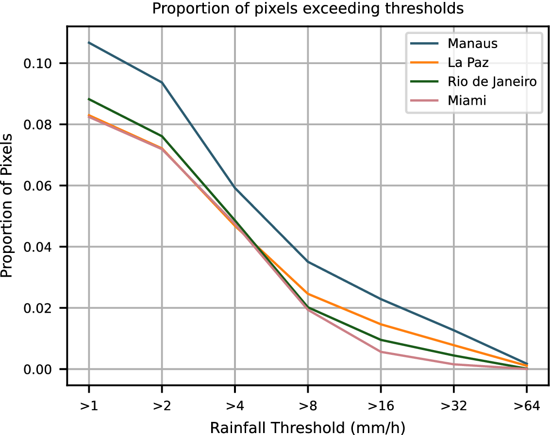
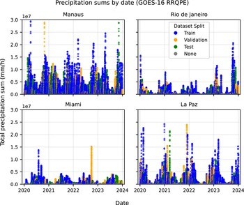
GOES-R Advanced Baseline Imager Rain Rate Quantitative Precipitation Estimation (RRQPE) (GOES-R Algorithm Working Group and GOES-R Program Office, 2018). RRQPE provides precipitation estimates over the Americas every 10 min at a spatial resolution with a latency of approximately 5 min, enabling real-time nowcasting. This product is highly correlated with rain-related bands and has been validated against ground radars and the GPM CORRA dataset (Agrawal et al., Reference Agrawal, Hassen, Brempong, Babenko, Zyda, Graham, Li, Merchant, Potes, Russell, Cheresnick, Kakkirala, Rasp, Hassidim, Matias, Kalchbrenner, Gupta, Hickey and Bell2025), highlighting the value of predicting geostationary satellite observations. We use RRQPE from January 2020 to December 2023. Rain events are defined as contiguous periods when the precipitation rate exceeds a chosen threshold (see Section 5.1 for details); we sample events uniformly at random and allocate 70% to training, 15% to validation, and 15% to testing. Figure 1 shows the proportion of observations above various thresholds for four different cities, while Figure 2 displays the accumulated precipitation and dataset splits.
Proportion of observations above different precipitation thresholds in the GOES-16 RRQPE dataset for each of the four study regions. Manaus exhibits the highest frequency of heavy rainfall across thresholds, while Rio de Janeiro and La Paz show intermediate levels.

Figure 1. Long description
The line graph is titled Proportion of pixels exceeding thresholds. The horizontal X axis is labeled Rainfall Threshold in m m forward slash h and features categorical points for greater than 1, greater than 2, greater than 4, greater than 8, greater than 16, greater than 32, and greater than 64. The vertical Y axis is labeled Proportion of Pixels and ranges from 0.00 to 0.10.
Four lines represent different study regions:
* Manaus (blue line) starts at the highest point of approximately 0.105 at the greater than 1 threshold and remains the uppermost line across the entire graph, ending near 0.002 at the greater than 64 threshold.
* La Paz (orange line) starts at 0.083 and follows a steady decline, staying above Rio de Janeiro and Miami after the greater than 4 threshold.
* Rio de Janeiro (dark green line) starts at 0.088, slightly higher than La Paz, but drops more sharply after the greater than 2 threshold, falling below La Paz at the greater than 8 mark.
* Miami (pink line) starts at 0.082 and exhibits the steepest decline, remaining the lowest line for all thresholds greater than 2.
All four regions show a non-linear, asymptotic decay toward zero as the rainfall intensity threshold increases.
Accumulated precipitation in GOES-16 RRQPE from January 2020 to December 2023 over each study region. Shaded areas denote training, validation, and test splits. Seasonal variability differs markedly between regions, with pronounced dry and wet seasons in La Paz and Rio de Janeiro.

Figure 2. Long description
A multi-panel graph with four subplots arranged in a two by two grid. The shared Y axis is labeled Total precipitation sum in millimeters per hour with a scale from 0.0 to 3.0 times 10 super 7. The shared X axis is labeled Date ranging from 2020 to 2024. A legend in the top right panel identifies Dataset Splits as blue for Train, orange for Validation, green for Test, and gray for None.
* Top-Left Panel Manaus. Shows high-frequency precipitation spikes throughout the year with peaks consistently reaching between 1.5 and 3.0 times 10 super 7. The data is predominantly blue Train with green Test data concentrated in late 2023.
* Top-Right Panel Rio de Janeiro. Displays distinct seasonal clusters. Peaks are lower than Manaus, mostly under 1.5 times 10 super 7, with a significant blue Train peak in early 2024 reaching 2.0.
* Bottom-Left Panel Miami. Shows the lowest overall precipitation sums among the four regions. Most data points remain below 0.5 times 10 super 7, with one notable orange Validation spike in late 2022 reaching 1.5.
* Bottom-Right Panel La Paz. Exhibits sharp, narrow seasonal spikes separated by dry periods. Peaks regularly reach between 1.5 and 2.5 times 10 super 7. The distribution includes blue Train, orange Validation, and green Test segments interspersed across the four-year period.
3.2. IMERG
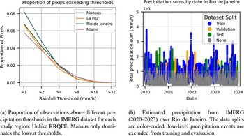
To test generalization across data sources, we also use the Integrated Multi-satellitE Retrievals for GPM (IMERG) Final Run product (Huffman et al., Reference Huffman, Bolvin, Braithwaite, Hsu, Joyce and Xie2014). IMERG provides precipitation estimates every 30 min at a resolution and is widely used in remote sensing research. Its latency is about 3.5 months (the Early Run version has 4 hour latency), which precludes real-time use but offers an independent validation dataset. We extract IMERG data from January 2020 to December 2023, split it using the same event-based procedure, and consider only the Rio de Janeiro region. Figure 3 compares the proportion of heavy-rain observations and accumulated precipitation for IMERG.
Statistics of IMERG data, highlighting differences with respect to the RRQPE dataset.

Figure 3. Long description
Panel a is a line graph titled Proportion of pixels exceeding thresholds. The horizontal axis represents Rainfall Threshold in millimeters per hour with categorical labels greater than 1, greater than 2, greater than 4, greater than 8, greater than 16, and greater than 32. The vertical axis represents Proportion of Pixels from 0.00 to 0.08. Four lines represent different cities. Manaus starts highest at 0.08 for the greater than 1 threshold but drops sharply to meet other cities by the greater than 4 threshold. La Paz, Rio de Janeiro, and Miami follow similar exponential decay curves, all converging near zero at the greater than 32 threshold.
Panel b is a scatter plot titled Precipitation sums by date in Rio de Janeiro. The horizontal axis shows years from 2020 to 2024. The vertical axis is Total precipitation sum in millimeters per hour, scaled by 10 to the 5 power. Data points are color-coded by Dataset Split. Blue dots represent Train data, orange dots represent Validation, green dots represent Test, and grey dots represent None. The grey points are concentrated at the bottom below 1 times 10 to the 5 power. Higher intensity events reaching up to 4 times 10 to the 5 power are distributed across the Train, Validation, and Test sets throughout the four-year period.
3.3. Study regions
To evaluate model performance across different climates, we select four
$ 512\;\mathrm{km}\times 512\;\mathrm{km} $
 subregions of the GOES-16 domain centered on Rio de Janeiro (Brazil), La Paz (Bolivia), Manaus (Brazil), and Miami (USA). These regions span coastal, high-altitude, rainforest, and subtropical environments. For IMERG, we consider only a
$ 2560\;\mathrm{km}\times 2560\;\mathrm{km} $
subregions of the GOES-16 domain centered on Rio de Janeiro (Brazil), La Paz (Bolivia), Manaus (Brazil), and Miami (USA). These regions span coastal, high-altitude, rainforest, and subtropical environments. For IMERG, we consider only a
$ 2560\;\mathrm{km}\times 2560\;\mathrm{km} $
 area surrounding Rio de Janeiro. The dominant precipitation processes include orographic and mesoscale convection in the Rio (Luiz-Silva and Oscar-Júnior, Reference Luiz-Silva and Oscar-Júnior2022), high-altitude convective storms in La Paz (Garreaud, Reference Garreaud2001), monsoon-driven convection in Manaus (Oliveira et al., Reference Oliveira, Maggioni, Vila and Morales2016) and sea-breeze thunderstorms in Miami (Burpee, Reference Burpee1979). Figure 2 illustrates the seasonal cycle and dataset splits for GOES-16 across regions.
4. Methods
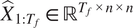
The proposed model, TUPANN, forecasts precipitation fields from a sequence of past satellite images
$ {X}_{-T:0}\in {\mathrm{\mathbb{R}}}^{\left(T+1\right)\times n\times n} $
 , where
$ n $
, where
$ n $
 denotes the spatial resolution (i.e., number of pixels per dimension) and
$ T+1 $
denotes the spatial resolution (i.e., number of pixels per dimension) and
$ T+1 $
 is the number of past observations. It produces predicted fields
$ {\hat{X}}_{1:{T}_f}\in {\mathrm{\mathbb{R}}}^{T_f\times n\times n} $
is the number of past observations. It produces predicted fields
$ {\hat{X}}_{1:{T}_f}\in {\mathrm{\mathbb{R}}}^{T_f\times n\times n} $
 , where
$ {T}_f $
, where
$ {T}_f $
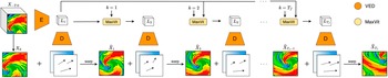
 is the forecast horizon. The architecture comprises two modules: (i) a variational encoder–decoder (VED) that learns a latent representation
$ {L}_k $
is the forecast horizon. The architecture comprises two modules: (i) a variational encoder–decoder (VED) that learns a latent representation
$ {L}_k $
 ,
$ k=1,\dots, {T}_f $
,
$ k=1,\dots, {T}_f $
 of the evolution of the precipitation fields under optical flow supervision; (ii) a visual transformer (MaxViT) that evolves the latent representation
$ {L}_k $
of the evolution of the precipitation fields under optical flow supervision; (ii) a visual transformer (MaxViT) that evolves the latent representation
$ {L}_k $
 so that the resulting application of a differentiable advection operator (warp) on the decoded motion and intensity fields,
$ {\hat{s}}_{k-1\to k} $
so that the resulting application of a differentiable advection operator (warp) on the decoded motion and intensity fields,
$ {\hat{s}}_{k-1\to k} $
 and
$ {\hat{v}}_{k-1\to k} $
and
$ {\hat{v}}_{k-1\to k} $
 , closely match the ground truth frame. See Figure 4. The training procedure is sequential: the VED module is initially trained to infer the first set of motion and intensity fields, then its weights are fixed and used for the training of the MaxVit module. Details on the VED and MaxViT training are discussed in Sections 4.1 and 4.2, respectively.
TUPANN architecture. The VED and MaxViT modules displayed are learned; motion fields and the final predictions are extrapolated through a warp function.

Figure 4. Long description
The flowchart begins on the far left with an input data cube labeled X sub negative T to zero. An arrow points down to a single frame X sub zero.
Top Track (Latent Processing):
The input cube passes through an orange trapezoid labeled E into a latent block L sub 1. A horizontal sequence follows where L sub 1 feeds into a MaxViT module at k equals 1, producing L sub 2. This pattern repeats for k equals 2 and k equals T sub f, with ellipses indicating intermediate steps. A skip connection line runs from the output of E across the top to each MaxViT module.
Bottom Track (Warping and Prediction):
Each latent block L sub n is connected to an orange trapezoid labeled D. The output of D is added to a motion field represented by vector arrows. This combined data passes through a warp function to generate a predicted frame.
- L sub 1 and D produce the first motion field, which warps X sub zero into X hat sub 1.
- L sub 2 and D produce the second motion field, which warps X hat sub 1 into X hat sub 2.
- This continues until the final prediction X hat sub T sub f is generated.
A legend on the top right identifies orange circles as V E D and light yellow circles as MaxViT.
Even though MaxViT offers linear complexity in the image size, the choice of such encoder–decoder architecture is guided by the idea that, apart from compressing the images, the VED is also responsible for learning the dynamics of a single-step evolution. MaxViT, on the other hand, learns to extrapolate the dynamics to further lead times.
4.1. Variational encoder–decoder
We use a variational encoder–decoder to learn an efficient representation of the precipitation evolution. Instead of reconstructing the input images as in classical variational autoencoders, our VED outputs motion fields
$ {\hat{v}}_{0\to 1}\in {\mathrm{\mathbb{R}}}^{2\times n\times n} $
 and intensity corrections
$ {\hat{s}}_{0\to 1}\in {\mathrm{\mathbb{R}}}^{n\times n} $
and intensity corrections
$ {\hat{s}}_{0\to 1}\in {\mathrm{\mathbb{R}}}^{n\times n} $
 given the past sequence
$ {X}_{-T:0} $
given the past sequence
$ {X}_{-T:0} $
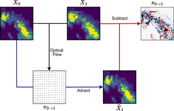
 . To enforce physically plausible motion, we compute the ground truth motion fields
$ {v}_{0\to 1} $
. To enforce physically plausible motion, we compute the ground truth motion fields
$ {v}_{0\to 1} $
 applying an optical flow algorithm to
$ {X}_{-\tilde{T}+2:1} $
applying an optical flow algorithm to
$ {X}_{-\tilde{T}+2:1} $
 , where
$ \tilde{T} $
, where
$ \tilde{T} $
 is the context length provided to the optical flow algorithm. After that, the ground truth intensity correction
$ {s}_{0\to 1} $
is the context length provided to the optical flow algorithm. After that, the ground truth intensity correction
$ {s}_{0\to 1} $
 is obtained by subtracting the advected frame
$ {\tilde{X}}_1 $
is obtained by subtracting the advected frame
$ {\tilde{X}}_1 $
 , obtained using
$ {v}_{0\to 1} $
, obtained using
$ {v}_{0\to 1} $
 , from the true frame
$ {X}_1 $
, from the true frame
$ {X}_1 $
 (see Figure 5). Thus, the estimated fields
$ {\hat{v}}_{0\to 1} $
(see Figure 5). Thus, the estimated fields
$ {\hat{v}}_{0\to 1} $
 and
$ {\hat{s}}_{0\to 1} $
and
$ {\hat{s}}_{0\to 1} $
 can be used to extrapolate the last observed frame
$ {X}_0 $
can be used to extrapolate the last observed frame
$ {X}_0 $
 to an estimate
$ {\hat{X}}_1 $
to an estimate
$ {\hat{X}}_1 $
 of the next frame via an advection operator (see Section 4.2.2).
Ground truth motion fields are obtained using an optical flow method from a pair of past and future images. The past image is advected to obtain an intermediate one,
$ {\tilde{X}}_1 $
 . Finally, ground truth intensity is the subtraction of
$ {\tilde{X}}_1 $
. Finally, ground truth intensity is the subtraction of
$ {\tilde{X}}_1 $
 from the future image.

4.1.1. Target loss
To supervise the predicted
$ {\hat{v}}_{0\to 1} $
 ,
$ {\mathrm{\ell}}_1 $
,
$ {\mathrm{\ell}}_1 $
 and cosine-similarity losses are used with respect to
$ {v}_{0\to 1} $
and cosine-similarity losses are used with respect to
$ {v}_{0\to 1} $
 . The intensity discrepancies between
$ {s}_{0\to 1} $
. The intensity discrepancies between
$ {s}_{0\to 1} $
 and
$ {\hat{s}}_{0\to 1} $
and
$ {\hat{s}}_{0\to 1} $
 are penalized via
$ {\mathrm{\ell}}_1 $
are penalized via
$ {\mathrm{\ell}}_1 $
 loss. Finally, a Kullback–Leibler divergence term is added to ensure the regularity of the learned latent space. The VED loss is

Here,
$ {\hat{p}}_{\theta } $
 is the latent distribution inferred by the encoder,
$ p $
is the latent distribution inferred by the encoder,
$ p $
 is a standard normal distribution and
$ {\lambda}_{\mathrm{int}},{\lambda}_{\mathrm{motion}},{\lambda}_{\mathrm{cos}},{\lambda}_{\mathrm{KL}} $
is a standard normal distribution and
$ {\lambda}_{\mathrm{int}},{\lambda}_{\mathrm{motion}},{\lambda}_{\mathrm{cos}},{\lambda}_{\mathrm{KL}} $
 are hyperparameters tuned on the validation set. This loss encourages accurate motion fields, intensity corrections, and latent regularity.
4.1.2. Optical flow
An optical flow algorithm is able to infer motion fields between two images, and is thus essential to obtain the derived ground-truth motion and intensity fields (e.g.,
$ {v}_{0\to 1},{s}_{0\to 1} $
 ) used in (1). We consider two options: Lucas–Kanade (LK), which solves a local least-squares problem under the assumption of small displacements, and DARTS, a spectral method tailored to radar imagery that solves the optical-flow equation in Fourier space. For TUPANN, we have taken the choice of optical flow method as a hyperparameter; below, we use DARTS for GOES-16 and LK for IMERG results.
4.2. MaxViT
Given the latent representation
$ {L}_1 $
 from the VED, a visual transformer evolves the latent state forward in time. We adopt MaxViT (Tu et al., Reference Tu, Talebi, Zhang, Yang, Milanfar, Bovik, Li, Avidan, Brostow, Cissé, Farinella and Hassner2022), which combines local and grid attention to efficiently capture global context while avoiding quadratic attention cost.
4.2.1. Lead time conditioning
To predict the latent state at the lead time
$ k $
 , we condition the transformer on
$ k $
, we condition the transformer on
$ k $
 via one-hot encoding and linear embedding, yielding
$ {L}_k=\mathrm{VT}\left({L}_1,k\right) $
via one-hot encoding and linear embedding, yielding
$ {L}_k=\mathrm{VT}\left({L}_1,k\right) $
 ,
$ k=2,\dots, {T}_f $
,
$ k=2,\dots, {T}_f $
 , where where
$ \mathrm{VT}\left(\cdot \right) $
, where where
$ \mathrm{VT}\left(\cdot \right) $
 represents the MaxViT model. Unlike recurrent decoding, this conditioning enables the same transformer to produce all lead times while reducing memory overhead (Andrychowicz et al., Reference Andrychowicz, Espeholt, Li, Merchant, Merose, Zyda, Agrawal and Kalchbrenner2023). Applying the VED decoder to
$ {L}_k $
represents the MaxViT model. Unlike recurrent decoding, this conditioning enables the same transformer to produce all lead times while reducing memory overhead (Andrychowicz et al., Reference Andrychowicz, Espeholt, Li, Merchant, Merose, Zyda, Agrawal and Kalchbrenner2023). Applying the VED decoder to
$ {L}_k $
 yields motion and intensity fields
$ \left({\hat{v}}_{k-1\to k},{\hat{s}}_{k-1\to k}\right)=D\left({L}_k\right) $
yields motion and intensity fields
$ \left({\hat{v}}_{k-1\to k},{\hat{s}}_{k-1\to k}\right)=D\left({L}_k\right) $
 , where
$ D\left(\cdot \right) $
, where
$ D\left(\cdot \right) $
 is the decoder module of the VED. Thus, all the necessary elements to predict the sequence recursively are obtained.
4.2.2. Warp function
Following NowcastNet (Zhang et al., Reference Zhang, Long, Chen, Xing, Jin, Jordan and Wang2023), we implement a fixed, differentiable advection operator that can reconstruct future precipitation frames using the predicted motion and intensity fields. Thus, given a frame
$ {\hat{X}}_{k-1} $
 , motion field
$ {\hat{v}}_{k-1\to k} $
, motion field
$ {\hat{v}}_{k-1\to k} $
 and intensity field
$ {\hat{s}}_{k-1\to k} $
and intensity field
$ {\hat{s}}_{k-1\to k} $
 , the extrapolated frame
$ {\hat{X}}_k $
, the extrapolated frame
$ {\hat{X}}_k $
 is
is

Roughly, following Zhang et al. (Reference Zhang, Long, Chen, Xing, Jin, Jordan and Wang2023), the warp function takes the image
$ {\hat{X}}_{k-1} $
 and applies the motion vector field
$ {\hat{v}}_{k-1\to k} $
and applies the motion vector field
$ {\hat{v}}_{k-1\to k} $
 pointwise; finally, the intensity field
$ {\hat{s}}_{k-1\to k} $
pointwise; finally, the intensity field
$ {\hat{s}}_{k-1\to k} $
 is added to the result.
4.2.3. Target loss
We compute the target loss in the original image space. We assume that
$ {\hat{X}}_{k-1}={X}_{k-1} $
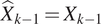 in equation (2) to avoid a costly recursive loss and calculate the
$ {\mathrm{\ell}}_1 $
in equation (2) to avoid a costly recursive loss and calculate the
$ {\mathrm{\ell}}_1 $
 loss between the warped frame
$ {\hat{X}}_k $
loss between the warped frame
$ {\hat{X}}_k $
 and the observed frame
$ {X}_k $
and the observed frame
$ {X}_k $
 . Thus,

The gradients of this loss will flow through the VED decoder module and the MaxViT transformer. The VED is pre-trained separately; thus, optimizing this loss only affects the MaxViT modules.
5. Experiments and results
We compare TUPANN against four nowcasting benchmarks using several evaluation metrics and across regions with different climates. We also run several ablation experiments.
5.1. Rain events dataset selection
The datasets used to train and evaluate our models comprise a subsample of rainy windows drawn from either the GOES-16 RRQPE or the IMERG products. We define a rainy window as follows. For each 10-min timestamp
$ t $
 from 2020-01-01 00:00 UTC to 2023-12-31 23:50 UTC, we (i) form a symmetric 60-min window
$ \left[t-30\;\min, t+30\;\min \right] $
from 2020-01-01 00:00 UTC to 2023-12-31 23:50 UTC, we (i) form a symmetric 60-min window
$ \left[t-30\;\min, t+30\;\min \right] $
 ; (ii) compute the spatiotemporal precipitation accumulation over that window (10-min steps over all grid points); and (iii) if the accumulation exceeds a threshold
$ \tau $
; (ii) compute the spatiotemporal precipitation accumulation over that window (10-min steps over all grid points); and (iii) if the accumulation exceeds a threshold
$ \tau $
 , label the larger window
$ \left[t-4\;\mathrm{hours},t+4\;\mathrm{hours}\right] $
, label the larger window
$ \left[t-4\;\mathrm{hours},t+4\;\mathrm{hours}\right] $
 as a rainy window. Finally, we merge rainy windows that intersect. The threshold
$ \tau =\mathrm{120,000} $
as a rainy window. Finally, we merge rainy windows that intersect. The threshold
$ \tau =\mathrm{120,000} $
 was chosen empirically to balance excluding near-dry periods against obtaining a dataset large enough for effective learning. Using a symmetric
$ \pm 4 $
was chosen empirically to balance excluding near-dry periods against obtaining a dataset large enough for effective learning. Using a symmetric
$ \pm 4 $
 -hour window ensures that events include both onset and dissipation phases (from no precipitation to mild or heavy precipitation and back).
5.2. Evaluation framework
We evaluate TUPANN and baselines using the critical success index (CSI) and Heidke skill score (HSS). Both metrics depend on a choice of threshold
$ t $
 , so that pixel values above the threshold are assigned as positive and, otherwise, negative. CSI and HSS are given by

where
$ \mathrm{TP} $
 stands for true positive,
$ \mathrm{TN} $
stands for true positive,
$ \mathrm{TN} $
 for true negatives,
$ \mathrm{FN} $
for true negatives,
$ \mathrm{FN} $
 for false negatives and
$ \mathrm{FP} $
for false negatives and
$ \mathrm{FP} $
 for false positives. Thus, CSI quantifies the overlap between forecasted and observed precipitation, ignoring true negatives (i.e., disregarding correct predictions of no precipitation) while HSS compares the forecast against random chance.
We report CSI and HSS at thresholds of 4, 8, 16, 32 and 64 mm/h and compute both pixel-wise scores (POOL1) and max-pooled scores over
$ 4\times 4 $
 blocks (POOL4). For aggregated metrics, we denote CSI–M and HSS–M as the mean across all thresholds. CSI values are reported in Section 5.4, and HSS ones are included in the Supplementary Materials.
5.3. Baseline models and tuning
In our experiments, TUPANN is compared with four baselines from different nowcasting paradigms:
-
• PySTEPS (LK) and PySTEPS (DARTS) (Pulkkinen et al., Reference Pulkkinen, Nerini, Pérez Hortal, Velasco-Forero, Seed, Germann and Foresti2019): optical-flow baselines that estimate a motion field (LK: local Lucas–Kanade; DARTS: DFT-based spectral) from recent frames and then semi-Lagrangianly advect the precipitation field forward. As purely physical extrapolation methods, they are strong for very short lead times;
-
• Earthformer (Gao et al., Reference Gao, Shi, Wang, Zhu, Wang, Li and Yeung2022): a space–time Transformer for Earth-system data that uses Cuboid Attention (local block attention with global tokens) in a hierarchical encoder–decoder to predict future frames;
-
• NowcastNet (Zhang et al., Reference Zhang, Long, Chen, Xing, Jin, Jordan and Wang2023): a hybrid model combining a U-Net–based learnable semi-Lagrangian advection (Evolution Network) with a physics-conditioned generative network trained with a temporal discriminator to inject high-resolution convective structure;
-
• CasCast (Gong et al., Reference Gong, Bai, Ye, Xu, Liu, Dai, Yang and Ouyang2024): a cascaded scheme that first uses a deterministic predictor (e.g., Earthformer) to capture mesoscale evolution, then conditions a latent-space diffusion transformer on that coarse forecast to generate small-scale features and improve extreme-precipitation skill.
For TUPANN and Earthformer, we tune learning rate, dropout rate, and loss weights on the validation set by maximizing mean CSI in the city of Rio de Janeiro, and use these for the other cities. The hyperparameters for NowcastNet and CasCast are those proposed in their original papers. The Supplementary Material to this article collects the final choice of hyperparameters for Earthformer and TUPANN. We trained each model for at most 20–300 epochs depending on the model, and chose the configuration that resulted in the highest CSI (averaged over thresholds). The optimizer for all models is Adam. After selecting the best values, we retrain on the combined training and validation data and evaluate on a held-out test set. Training uses a single NVIDIA A100 GPU, and inference typically takes under 2 seconds per forecast (for all 18 lead times).
5.4. GOES-16 results
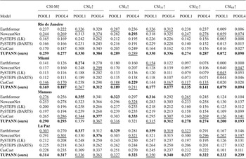
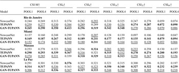
Table 1 presents CSI scores across the four study regions and thresholds. TUPANN consistently ranks first or second for each metric. In Rio de Janeiro, it achieves the highest CSI at all thresholds; NowcastNet is the closest competitor, followed by Earthformer. In Miami, TUPANN again dominates most metrics, but now CasCast performs well. In Manaus and La Paz, Earthformer and NowcastNet obtain slightly better CSI for low thresholds, but TUPANN leads for higher thresholds and is therefore better at forecasting extreme rainfall. The 64 mm/h CSI values are small across models, reflecting the rarity of such intense events, yet TUPANN’s scores remain the highest. Overall, the table highlights TUPANN’s performance across different climate regimes and precipitation thresholds. Similar results are true for HSS (see Supplementary Material), although by that metric, Earthformer is much more competitive.
Aggregated CSI metrics for GOES-16 data across cities

Table 1. Long description
The table presents Critical Success Index (C S I) metrics across six categories: C S I M, C S I 4, C S I 8, C S I 16, C S I 32, and C S I 64, each subdivided into POOL1 and POOL4.
* Rio de Janeiro: T U P A N N (ours) achieves the highest scores in almost all categories, including C S I M (0.259 for POOL1, 0.277 for POOL4) and C S I 64 (0.072 for POOL1, 0.090 for POOL4). NowcastNet is frequently the second-best performer.
* Miami: T U P A N N (ours) leads in most categories, such as C S I M (0.169 for POOL1, 0.187 for POOL4) and C S I 64 (0.079 for POOL1, 0.094 for POOL4). CasCast and Earthformer show competitive results in lower thresholds like C S I 4.
* Manaus: T U P A N N (ours) shows top performance in C S I M (0.290 for POOL1) and C S I 64 (0.200 for POOL1, 0.193 for POOL4). Earthformer and CasCast perform well in the C S I 4 and C S I 8 categories.
* La Paz: T U P A N N (ours) leads in C S I M (0.314 for POOL1, 0.317 for POOL4) and C S I 64 (0.232 for POOL1, 0.239 for POOL4). Earthformer and NowcastNet are the primary competitors in the middle thresholds.
Across all regions, T U P A N N consistently shows state-of-the-art performance, particularly at higher rain-rate thresholds (C S I 32 and C S I 64).
Note: Bold values denote the best, underlined values the second best. TUPANN obtains state-of-the-art performance at most thresholds and regions, particularly for high rain-rate events.
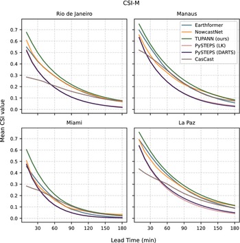
The graphs in Figure 6 show mean CSI (averaged across thresholds) versus lead time. TUPANN maintains the highest or second-highest skill across all lead times; the advantage over NowcastNet grows for early lead times, reflecting the benefit of explicit motion supervision and the efficiency of lead-time conditioning (see also Figure 7).
Mean CSI (CSI–M) versus lead time for the four study regions using GOES-16 data. TUPANN consistently outperforms baselines across lead times.

Figure 6. Long description
The figure consists of four panels arranged in a two by two grid. Each panel shares a common Y axis labeled Mean C S I value ranging from 0.0 to 0.7 and a common X axis labeled Lead Time min ranging from 30 to 180.
* Top-Left Panel Rio de Janeiro. T U P A N N starts at the highest point near 0.7 and follows a decaying curve. Earthformer and NowcastNet follow closely below. Py S T E P S D A R T S shows the steepest decline, while CasCast starts much lower at 0.3 and has the flattest slope, intersecting other models around the 60 minute mark.
* Top-Right Panel Manaus. All models start higher than in Rio. T U P A N N remains the top curve throughout the 180 minute duration. Earthformer and NowcastNet are nearly identical in the middle range. Py S T E P S L K and D A R T S occupy the lowest performance positions.
* Bottom-Left Panel Miami. Initial C S I values are lower overall, with T U P A N N starting at 0.6. The curves converge more tightly as lead time increases toward 180 minutes, where all values drop below 0.1.
* Bottom-Right Panel La Paz. T U P A N N shows a distinct lead over the other models. Similar to Rio, CasCast starts at a lower value of 0.4 but maintains a more stable, linear decline compared to the exponential decay of the other models.
A legend in the top-right panel identifies the six models. Earthformer in blue, NowcastNet in orange, T U P A N N ours in green, Py S T E P S L K in pink, Py S T E P S D A R T S in purple, and CasCast in brown.
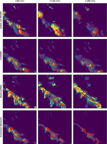
Comparison of motion fields. Top row: GOES-16 RRQPE observations (ground truth) overlaid by ground-truth DARTS motion fields for future frames. Subsequent rows: learned motion fields from TUPANN, NowcastNet, and Evolution Network. In all frames, red arrows represent the motion fields. TUPANN yields smoother fields that align with physical intuition.

Figure 7. Long description
A multi-panel visualization organized into four rows and three columns. The columns are labeled from left to right as plus 60 min, plus 120 min, and plus 180 min.
* The first row, labeled G O E S 16 R R Q P E, shows ground truth data with dense red arrows indicating motion fields over yellow and green precipitation clusters on a dark blue background. The motion is generally directed toward the Southeast.
* The second row, labeled T U P A N N, displays smoother, more continuous motion fields. The red arrows are more uniform in direction compared to the ground truth, following the general Southeast flow with less local turbulence.
* The third row, labeled NowcastNet, shows motion fields that are more fragmented and varied in direction than T U P A N N, with arrows appearing more concentrated on the leading edges of the precipitation bands.
* The fourth row, labeled Evolution Network, shows the most sparse motion fields. The red arrows are primarily clustered around the most intense precipitation areas, with fewer arrows in the peripheral regions compared to the other models.
Across all rows, the precipitation clusters shift from the Northwest toward the Southeast as time progresses from the first to the third column.
Beyond aggregated metrics, a large-scale illustration of TUPANN’s prediction for a rain event in Manaus, compared with NowcastNet, CasCast, and Earthformer, is included in the Supplementary Material. Generative models such as NowcastNet and CasCast produce detailed textures but may introduce artifacts, whereas TUPANN and Earthformer yield smoother predictions. Despite the blurred appearance, TUPANN captures the timing and location of heavy rain more accurately, leading to higher CSI values.
5.5. Ablation results
We will study how different experiments affect TUPANN: investigating its motion fields against another physics-DL hybrid model, adding a GAN head, evaluating TUPANN’s cross-city generalization, and training the model jointly on all cities.
5.5.1. Interpretability and motion fields
TUPANN’s interpretability stems from its explicitly learned motion fields. Figure 7 compares motion fields predicted by TUPANN and NowcastNet (which relies on an Evolution Network submodule for its motion fields). The TUPANN fields are smooth and closely resemble the numerical optical flow computed by DARTS, whereas the baselines’ fields exhibit unrealistic patterns. This underscores the benefit of supervising motion fields directly.
5.5.2. GAN-TUPANN
Generative adversarial networks can improve visual realism at the cost of evaluation metrics. To study its impact on TUPANN predictions, we evaluate the variant GAN-TUPANN, which adds a GAN head to TUPANN outputs.
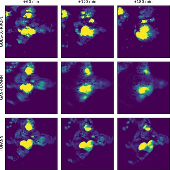
Figure 8 shows that GAN-TUPANN produces significantly sharper images. Still, Table 2 shows this does not always lead to improvements in CSI scores. While in Rio de Janeiro, GAN-TUPANN increases low-threshold CSI, in Miami, the gains are either non-existent or negative. Given the computational overhead and mixed impact on metrics, there is no clear advantage in including this module unless visual fidelity is paramount.
Visual comparison of TUPANN and GAN-TUPANN for a rain event in Rio de Janeiro, starting at 2023-03-11 03:00 UTC. The first row shows the GOES-16 RRQPE observations (ground truth). GAN-TUPANN reduces blur, but yields mixed changes in CSI (Table 2).

Figure 8. Long description
The grid consists of three rows and three columns. The columns are labeled from left to right as plus 60 min, plus 120 min, and plus 180 min.
Row 1 is labeled G O E S dash 16 R R Q P E. It shows the ground truth observations with high-contrast yellow clusters representing intense precipitation against a dark purple background. The central cluster expands and becomes more defined from the 60-minute to the 180-minute mark.
Row 2 is labeled G A N dash T U P A N N. These panels show a smoother, more blurred representation of the precipitation clusters compared to the ground truth. The yellow cores are less distinct and surrounded by larger gradients of teal and green.
Row 3 is labeled T U P A N N. These panels show sharper, more segmented precipitation clusters than the G A N dash T U P A N N row, though they appear slightly more fragmented than the G O E S dash 16 ground truth.
Across all rows, the primary precipitation feature moves slightly from the center toward the East and Southeast over the three-hour period.
CSI metrics comparing TUPANN and its GAN variant (GAN-TUPANN) on GOES-16 data

Table 2. Long description
The table presents Critical Success Index (C S I) metrics for three models: NowcastNet, T U P A N N, and G A N T U P A N N. The metrics include C S I M, C S I sub 4, C S I sub 8, C S I sub 16, C S I sub 32, and C S I sub 64, each evaluated with P O O L 1 and P O O L 4 methods.
* Rio de Janeiro: G A N T U P A N N achieves the highest scores for C S I M (0.265 for P O O L 1, 0.290 for P O O L 4), C S I sub 4 (0.350, 0.413), and C S I sub 8 (0.296, 0.319). T U P A N N performs best for C S I sub 32 (0.274, 0.287) and C S I sub 64 (0.072, 0.090).
* Miami: T U P A N N consistently outperforms other models across all metrics, with values such as 0.169 for C S I M P O O L 1 and 0.094 for C S I sub 64 P O O L 4.
* Manaus: T U P A N N leads in most categories, including C S I M (0.290, 0.293) and C S I sub 64 (0.200, 0.193), while G A N T U P A N N shows strength in C S I sub 8 (0.318, 0.329).
* La Paz: T U P A N N and G A N T U P A N N show competitive results. T U P A N N leads in C S I M (0.314, 0.317) and C S I sub 64 (0.232, 0.239), while NowcastNet records the highest C S I sub 4 P O O L 4 at 0.376.
Bold values indicate the best performance, and underlined values indicate the second best.
Note: Bold values denote the best, underlined values the second best. GAN-TUPANN improves low-threshold performance in Rio de Janeiro but degrades or yields marginal improvements in other cities.
5.5.3. Cross-city generalization
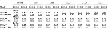
To assess generalization we train TUPANN on one city and evaluate on others. Table 3 compares TUPANN trained on Rio de Janeiro (TUPANN–Rio) against models trained separately on each city. In Manaus and La Paz, TUPANN–Rio yields lower CSI at all thresholds, as expected due to climate differences. Surprisingly, in Miami, the Rio-trained model performs comparably or better at high thresholds, possibly because heavy-rain events are rare in Miami (see Figure 1) and the Rio model may be biased towards such events. Overall, cross-city degradation is modest (at most
$ 20\% $
 ) and TUPANN–Rio still outperforms or matches baselines trained on the target city, highlighting the transferability of the architecture.
Cross-city CSI comparison between TUPANN trained on each city and TUPANN trained on Rio de Janeiro (TUPANN–Rio)
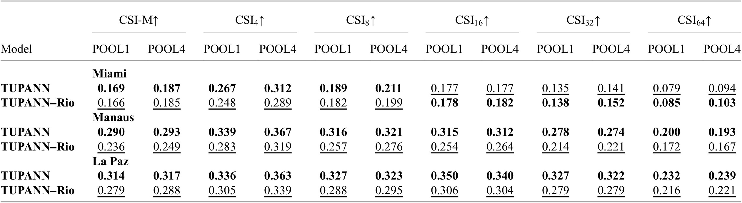
Table 3. Long description
The table is structured with a header row defining the Model and six C S I metrics, each with two sub-columns for P O O L 1 and P O O L 4. The metrics are C S I dash M, C S I sub 4, C S I sub 8, C S I sub 16, C S I sub 32, and C S I sub 64, all with up arrows indicating higher values are better.
For Miami:
* T U P A N N: C S I dash M (0.169, 0.187), C S I sub 4 (0.267, 0.312), C S I sub 8 (0.189, 0.211), C S I sub 16 (0.177, 0.177), C S I sub 32 (0.135, 0.141), C S I sub 64 (0.079, 0.094).
* T U P A N N Rio: C S I dash M (0.166, 0.185), C S I sub 4 (0.248, 0.289), C S I sub 8 (0.182, 0.199), C S I sub 16 (0.178, 0.182), C S I sub 32 (0.138, 0.152), C S I sub 64 (0.085, 0.103).
For Manaus:
* T U P A N N: C S I dash M (0.290, 0.293), C S I sub 4 (0.339, 0.367), C S I sub 8 (0.316, 0.321), C S I sub 16 (0.315, 0.312), C S I sub 32 (0.278, 0.274), C S I sub 64 (0.200, 0.193).
* T U P A N N Rio: C S I dash M (0.236, 0.249), C S I sub 4 (0.283, 0.319), C S I sub 8 (0.257, 0.276), C S I sub 16 (0.254, 0.264), C S I sub 32 (0.214, 0.221), C S I sub 64 (0.172, 0.167).
For La Paz:
* T U P A N N: C S I dash M (0.314, 0.317), C S I sub 4 (0.336, 0.363), C S I sub 8 (0.327, 0.323), C S I sub 16 (0.350, 0.340), C S I sub 32 (0.327, 0.322), C S I sub 64 (0.232, 0.239).
* T U P A N N Rio: C S I dash M (0.279, 0.288), C S I sub 4 (0.305, 0.339), C S I sub 8 (0.288, 0.295), C S I sub 16 (0.306, 0.304), C S I sub 32 (0.279, 0.279), C S I sub 64 (0.216, 0.221).
Note: Bold values denote the best, underlined values the second best. Cross-city performance declines in Manaus and La Paz but remains competitive; in Miami TUPANN–Rio improves high-threshold scores.
5.5.4. Multi-city training
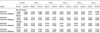
Rather than training a model for each city, training on multiple cities can further improve skill. Table 4 compares TUPANN trained separately on each city with a multi-city model trained jointly on all regions (including Toronto, see Supplementary Material). The multi-city model (TUPANN–Multicity) yields higher CSI across most thresholds and regions. Access to diverse climates helps the network learn more generalizable features, especially for extreme rainfall events.
Comparison between single-city TUPANN and a multi-city version (TUPANN–Multicity) trained on all regions simultaneously

Table 4. Long description
The table compares two models: T U P A N N and T U P A N N Multicity. The columns represent metrics: C S I hyphen M up-arrow, C S I sub 4 up-arrow, C S I sub 8 up-arrow, C S I sub 16 up-arrow, C S I sub 32 up-arrow, and C S I sub 64 up-arrow. Each metric is subdivided into P O O L 1 and P O O L 4 columns.
For Rio de Janeiro:
* T U P A N N: C S I hyphen M (0.259, 0.277), C S I sub 4 (0.330, 0.384), C S I sub 8 (0.289, 0.289), C S I sub 16 (0.330, 0.336), C S I sub 32 (0.274, 0.287), C S I sub 64 (0.072, 0.090).
* T U P A N N Multicity: C S I hyphen M (0.271, 0.286), C S I sub 4 (0.337, 0.390), C S I sub 8 (0.303, 0.297), C S I sub 16 (0.353, 0.353), C S I sub 32 (0.293, 0.304), C S I sub 64 (0.071, 0.086).
For Miami:
* T U P A N N: C S I hyphen M (0.169, 0.187), C S I sub 4 (0.267, 0.312), C S I sub 8 (0.189, 0.211), C S I sub 16 (0.177, 0.177), C S I sub 32 (0.135, 0.141), C S I sub 64 (0.079, 0.094).
* T U P A N N Multicity: C S I hyphen M (0.178, 0.190), C S I sub 4 (0.273, 0.313), C S I sub 8 (0.196, 0.211), C S I sub 16 (0.188, 0.182), C S I sub 32 (0.151, 0.151), C S I sub 64 (0.082, 0.095).
For Manaus:
* T U P A N N: C S I hyphen M (0.290, 0.293), C S I sub 4 (0.339, 0.367), C S I sub 8 (0.316, 0.321), C S I sub 16 (0.315, 0.312), C S I sub 32 (0.278, 0.274), C S I sub 64 (0.200, 0.193).
* T U P A N N Multicity: C S I hyphen M (0.291, 0.296), C S I sub 4 (0.340, 0.369), C S I sub 8 (0.316, 0.324), C S I sub 16 (0.314, 0.314), C S I sub 32 (0.278, 0.275), C S I sub 64 (0.208, 0.198).
For La Paz:
* T U P A N N: C S I hyphen M (0.314, 0.317), C S I sub 4 (0.336, 0.363), C S I sub 8 (0.327, 0.323), C S I sub 16 (0.350, 0.340), C S I sub 32 (0.327, 0.322), C S I sub 64 (0.232, 0.239).
* T U P A N N Multicity: C S I hyphen M (0.324, 0.325), C S I sub 4 (0.339, 0.363), C S I sub 8 (0.334, 0.327), C S I sub 16 (0.359, 0.348), C S I sub 32 (0.335, 0.331), C S I sub 64 (0.251, 0.254).
Note: Bold denotes the best, underlined the second best. The multi-city model improves performance in most cases, demonstrating the benefit of pooled training.
5.6. IMERG results
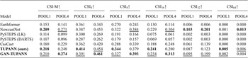
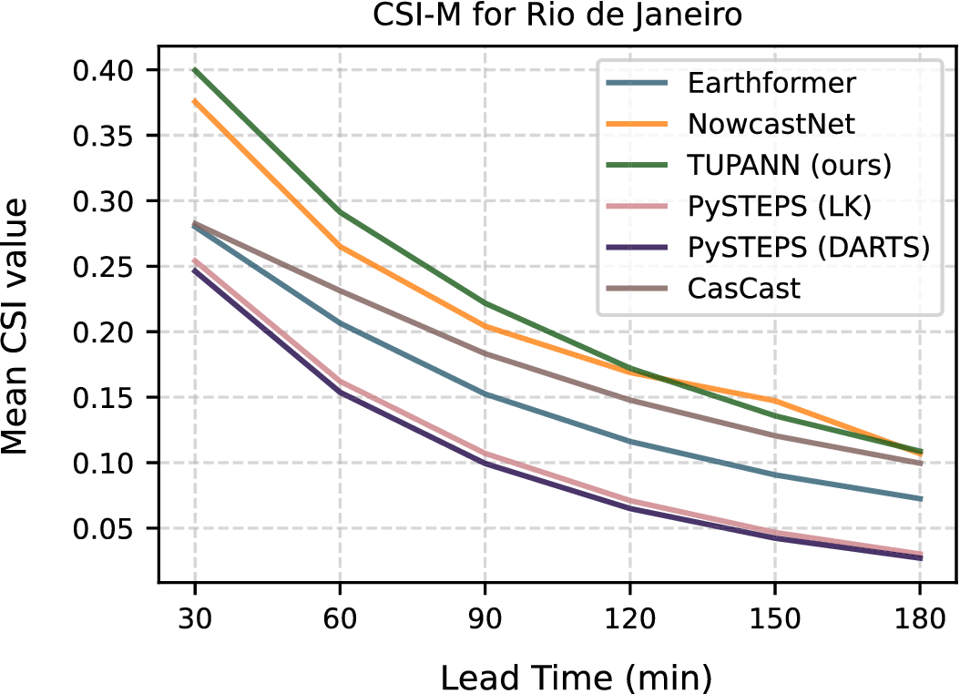
Table 5 compares TUPANN to baselines on the IMERG dataset for Rio de Janeiro. Without pooling (POOL1), TUPANN achieves the best CSI across all thresholds. With pooling (POOL4), generative models (NowcastNet, GAN-TUPANN) slightly outperform TUPANN at low thresholds, but TUPANN remains competitive and leads at higher thresholds. Figure 9 plots CSI–M versus lead time, showing TUPANN’s superior performance at most lead times and small gaps only at 150 minutes. These results demonstrate that TUPANN generalizes to coarser spatial resolution and longer latency datasets, where its physics-aligned architecture can become slightly less beneficial.
Aggregated CSI metrics for Rio de Janeiro using IMERG data

Table 5. Long description
The table consists of 13 columns. The first column lists the models: Earthformer, NowcastNet, PySTEPS open parenthesis L K close parenthesis, PySTEPS open parenthesis D A R T S close parenthesis, CasCast, T U P A N N open parenthesis ours close parenthesis, and G A N dash T U P A N N.
The header row defines six C S I metrics, each with an upward arrow indicating higher is better: C S I dash M, C S I sub 4, C S I sub 8, C S I sub 16, C S I sub 32, and C S I sub 64. Each metric is subdivided into two columns: P O O L 1 and P O O L 4.
Key data points include:
* C S I dash M: T U P A N N leads at P O O L 1 with 0.218, while G A N dash T U P A N N leads at P O O L 4 with 0.274.
* C S I sub 4: T U P A N N leads at P O O L 1 with 0.414, while G A N dash T U P A N N leads at P O O L 4 with 0.461.
* C S I sub 8: T U P A N N leads at P O O L 1 with 0.344, while G A N dash T U P A N N leads at P O O L 4 with 0.393.
* C S I sub 16: T U P A N N leads at P O O L 1 with 0.241, while G A N dash T U P A N N leads at P O O L 4 with 0.313.
* C S I sub 32: NowcastNet leads at both P O O L 1 with 0.103 and P O O L 4 with 0.201.
* C S I sub 64: T U P A N N leads at P O O L 1 with 0.005, while NowcastNet leads at P O O L 4 with 0.013.
Values for PySTEPS and Earthformer are generally lower across all thresholds. Bold text indicates the best performance and underlining indicates the second best.
Note: Bold denotes the best, underlined the second best. Without pooling TUPANN is clearly superior; with pooling, generative baselines perform slightly better at low thresholds, but TUPANN remains competitive overall.
Mean CSI versus lead time for IMERG data in Rio de Janeiro. TUPANN outperforms baselines at most lead times; NowcastNet overtakes slightly at 150 min but lags at shorter lead times.

Figure 9. Long description
The horizontal X-axis represents Lead Time in minutes with markers at 30, 60, 90, 120, 150, and 180. The vertical Y-axis represents Mean C S I value ranging from 0.05 to 0.40. All models show a downward trend as lead time increases.
* T U P A N N (ours) starts highest at 0.40 and remains the top performer until 150 minutes, where it is slightly overtaken by NowcastNet, ending at approximately 0.11.
* NowcastNet starts at 0.375 and follows a similar decay curve, crossing above T U P A N N at the 150-minute mark.
* CasCast starts at 0.28 and maintains a middle-tier position, ending at 0.10.
* Earthformer starts at 0.28, overlapping with CasCast initially, but drops more steeply to end at 0.07.
* P y S T E P S L K starts at 0.25 and ends at 0.03.
* P y S T E P S D A R T S starts at 0.245 and remains the lowest performer throughout, ending just below 0.03.
5.7. Operational deployment
Downloading and processing GOES-16 data and making predictions can be done in less than 3 minutes. Due to its low latency, this enables an efficient near real-time 10 to 180 minutes nowcast with 10 minutes temporal resolution. The whole pipeline, including the predictions generated by TUPANN, can be run on a machine with relatively modest requirements: 16GB of memory, a GeForce RTX 3080 GPU. Predictions can also include the derived motion fields to help meteorologists interpret the results. This system is currently operational and has been deployed to aid Rio de Janeiro’s Instituto Estadual do Ambiente (INEA) agency to prepare for floods and other extreme precipitation disasters. Due to TUPANN’s reliance on widely available geostationary satellite data, we expect that this solution can be broadened to other regions as well.
6. Limitations and future work
Our study has important limitations. First, although TUPANN may use globally available satellite products, this work relies on GOES-16 coverage for real-time nowcasting. Still, our results show that the model is able to adapt to different locations. It is straightforward to retrain TUPANN to other regions such as Europe and Africa (through the EUMETSAT Meteosat series satellites products, such as P-IN-SEVIRI-PMW (H60B) (EUMETSAT H SAF, 2022)) and Eastern Asia and Western Pacific (through the Himawari satellites, from the Japanese Meteorological Agency, and GK-2A, from the Korea Meteorological Administration). Second, the optical-flow supervision requires additional computation and may not perfectly capture complex convection dynamics; using the proposed scheme with additional covariates could yield further improvements under a more detailed physical modeling. Third, CSI and HSS values decline at longer lead times (>2 h), reflecting inherent predictability limits; integrating uncertainty quantification and ensemble approaches may better characterize forecast skill. Finally, GAN-based enhancements improve visual realism but degrade or inconsistently affect skill metrics; stabilizing adversarial training and assessing perceptual quality remain open challenges.
Future work includes coupling TUPANN with probabilistic post-processing to provide calibrated uncertainty estimates, extending the model to include additional inputs such as cloud imagery or microwave precipitation retrievals, and investigating transfer learning across continents.
7. Conclusions
We have presented TUPANN, a physically aligned neural network for precipitation nowcasting using satellite imagery. TUPANN’s modular design—combining a variational encoder–decoder supervised by optical flow, and a transformer capable of evolving the latent representation according to physical constraints—yields interpretable motion fields and competitive forecast skill. Extensive experiments on GOES-16 and IMERG data across four climates show that TUPANN matches or surpasses state-of-the-art baselines, particularly at high precipitation thresholds. Training in multiple cities improves performance, and cross-city evaluations reveal modest degradation, highlighting the model’s transferability. With its low latency and reliance on globally available satellites, TUPANN supports equitable access to short-term rainfall forecasts and provides a foundation for operational applications in radar-sparse regions.
Open peer review
To view the open peer review materials for this article, please visit http://doi.org/10.1017/eds.2026.10039.
Supplementary material
The supplementary material for this article can be found at http://doi.org/10.1017/eds.2026.10041.
Acknowledgements
The authors thank Adriana Monteiro, João Vitor Romano, Lucas Nissenbaum, and Thiago Ramos, as well as the help and support from Google, in particular, Shreya Agrawal, Boris Babenko, and Samier Merchant.
Author contribution
Conceptualization: A.C., M.P., L.V., P.O.; Data curation and visualization: A.C.; Methodology: A.C., M.P., L.V.; Writing—original draft: A.C., M.P., L.V.; Writing—review and editing: A.C., M.P., L.V., P.O. All authors approved the final manuscript.
Competing interests
The authors declare no competing interests.
Data availability statement
GOES-16 RRQPE data were obtained from the NOAA GOES-R Product Distribution and Access (PDA) system. IMERG Final Run data were obtained from the NASA GPM data portal. Processed datasets, event splits, and TUPANN code are available at Zenodo under the DOI 10.5281/zenodo.20349104 (Catão et al., Reference Catão, Poveda Quimiz, de Andrade and Orenstein2026).
Ethics statement
The research meets all ethical guidelines, including adherence to the legal requirements of Brazil and the United States.
Funding statement
A.C. was supported by a “FAPERJ Nota 10” grant (SEI-260003/004731/2025) from Fundação de Amparo à Pesquisa do Estado do Rio de Janeiro (FAPERJ). M.P. and L.V. were supported by scholarships from Coordenação de Aperfeiçoamento de Pessoal de Nível Superior (CAPES). P.O. was supported by grant SEI-260003/001545/2022 from FAPERJ.




 Open access


Comments
22 October 2025
Prof. Claire Monteleoni, Editor-in-Chief
Environmental Data Science (Cambridge University Press)
Dear Prof. Monteleoni and Editorial Team,
Please find our Methods Paper, “Precipitation nowcasting of satellite data using physically-aligned neural networks,” submitted for consideration in Environmental Data Science for the Climate Informatics 2025 track. Our manuscript introduces TUPANN (Transferable and Universal Physics-Aligned Nowcasting Network), a satellite-only deep learning system that generates 10–180-minute precipitation nowcasts without relying on radar networks. Since many high-risk regions lack the radar infrastructure behind current nowcasting solutions, our work broadens access to timely storm and flood alerts, strengthening emergency management and supporting urban drainage and transport operation in radar-limited regions.
TUPANN explicitly aligns learning with physical structure: a variational encoder–decoder module recovers motion and intensity under optical-flow supervision, a lead-time-conditioned MaxViT advances the latent state, and a differentiable advection operator reconstructs future frames. Unlike other state-of-the-art nowcasting methods, our physics-aligned decomposition yields interpretable motion fields and near-real-time operation from geostationary satellite inputs. Given EDS’s emphasis on AI/ML methods that advance environmental forecasting and decision-making, and the journal’s category of Methods papers, we believe the contribution is a strong match for your readership.
We evaluate on GOES-16 RRQPE and IMERG, across four contrasting climates (Rio de Janeiro, Manaus, Miami, La Paz) and show that TUPANN achieves the best or second-best skill against optical-flow, deep learning, and hybrid baselines, with pronounced gains at higher rain-rate thresholds. Multi-city training improves performance, and cross-city tests show occasional gains for heavy-rain regimes, supporting transferability. Operationally, TUPANN’s latency and refresh enable timely flood and storm alerts where radar is scarce, complementing existing NWP and radar products. To support transparency and reuse, we provide dataset access, event splits, and code, openly available at https://github.com/acataos/tupann.
We appreciate your consideration and would be delighted to see this work reach EDS’s community of researchers and practitioners working at the intersection of environmental science and data science.
Sincerely,
Antônio Catão, Melvin Poveda, Leonardo Voltarelli, and Paulo Orenstein