

INTRODUCTION
The changing sea-ice conditions in the Arctic (e.g. Perovich and others, Reference Perovich2016) are of interest for shipping companies, fishery, the oil and gas industry, and local residents. For operational ice charting and forecasts covering navigational and safety issues it is important to know about the state and the composition of the sea-ice cover. Additionally, knowledge about the ongoing changes in the Arctic like i.e. the decreasing sea-ice extent (e.g. Meier and others, Reference Meier2014) and sea-ice thickness (e.g. Ricker and others, Reference Ricker2017a,Reference Rickerb) are essential to understand the role of sea ice for the global climate system.
Recent work has focused on the retrieval of Arctic-wide sea-ice thickness estimates from direct observations (e.g. Lindsay and Schweiger, Reference Lindsay and Schweiger2015), from altimetry data (e.g. Kwok and Cunningham, Reference Kwok and Cunningham2015), and from altimetry data in combination with radiometric data (Kaleschke and others, Reference Kaleschke2015; Ricker and others, Reference Ricker2017b). The spatial variability of ice thickness, which may be related to sea-ice classes (Armstrong, Reference Armstrong1972), varies on a local and regional scale. Synthetic aperture radar (SAR) imagery provides regular information about the state of the Arctic sea-ice cover with high resolution on a local scale, unaffected by the occurrence of clouds or the absence of illumination on the surface. SAR images can be segmented into clusters with similar characteristics, and those clusters subsequently labeled or classified into categories. The segmentation and subsequent classification can be done using a number of different techniques, i.e. segmentation (Doulgeris and Eltoft, Reference Doulgeris and Eltoft2010; Doulgeris, Reference Doulgeris2013) followed by visual inspection (Hughes and Wagner, Reference Hughes and Wagner2015), neural network approaches (e.g. Hara and others, Reference Hara1995; Zakhvatkina and others, Reference Zakhvatkina, Alexandrov, Johannessen, Sandven and Frolov2013; Ressel and others, Reference Ressel, Singha, Lehner, Rösel and Spreen2016), the use of calibrated backscattering coefficients for discrimination between sea-ice classes (Johannessen and others, Reference Johannessen2007; Casey and others, Reference Casey, Howell, Tivy and Haas2016), and image texture analysis, such as Markov random fields (e.g. Yu and Clausi, Reference Yu and Clausi2007; Doulgeris, Reference Doulgeris2015).
The categories used in a classification can be based on the relationship between prominent sea-ice features (i.e. pressures ridges and open leads) and different ice types (i.e. deformed ice and new ice). In some, but by no means all, cases ice types can be related to ice thickness (e.g. young level ice, heavily deformed multi-year ice) (Armstrong, Reference Armstrong1972). In this study, we will distinguish between predominantly thin ice, level ice and deformed ice and validate the percentage of each class in a satellite image.
There is a natural limitation on the retrieval of sea-ice thickness from SAR due to saturation, with the greatest sensitivity below ~0.5 m for L-band SAR (e.g. Wakabayashi and others, Reference Wakabayashi, Matsuoka, Nakamura and Nishiro2004; Johansson and others, Reference Johansson2017). However, differences in sea-ice surface roughness, connected to different sea-ice classes, can be determined from SAR backscatter.
In this paper, the only class we identify from SAR that can be directly related to sea-ice thickness is that of thin ice (Johansson and others, Reference Johansson2017). Ridges and thicker sea ice can be separated from other sea-ice classes due to their brightness and radar image texture.
Different measurements on different nested scales can be used to validate each other. In situ ice thickness measurements at the kilometer scale can be compared with airborne sea-ice thickness data at a 10-km scale to determine whether they are representative of a wider area. In order to extend our understanding of sea-ice conditions to the satellite scale, is is necessary to ascertain how well those in situ and airborne measurements represent the different classes that can be identified following segmentation and analysis of the image. At the same time, the in situ data are used to validate the interpretation of the information derived from the SAR imagery, thus knowledge about the sea-ice situation and the availability of in situ observations is essential for validation and comparison studies with remote sensing and sea-ice modeling. Several questions arise about the relationship between measurements made at different scales: I.e., how do ground-based total sea-ice thickness measurements compare with airborne total sea-ice thickness data? How representative are these local scale measurements of a wider region? And, is it possible to define regions with similar sea-ice conditions from satellite images?
In this case study, we use extensive ground-based and airborne in situ observations from the Norwegian young sea ICE expedition (N-ICE2015), led by the Norwegian Polar Institute in the region north of Svalbard, from January to June 2015 (Granskog and others, Reference Granskog2016), and compare those with a segmented and classified ALOS-2 Palsar-2 SAR, L-band (ALOS-2) scene from 23 April 2015. A point-to-point comparison of in situ measurements on drifting sea ice to satellite pixels is challenging, especially when the time difference exceeds the suggested 3 h (Pope and others, Reference Pope2017). Instead, we focus below on the statistical comparison of the spatial occurrence of three defined simplified classes: ‘thin’, ‘level’, and ‘deformed’ within the different datasets and within different regions of the study area.
DATA AND METHODS
Study area
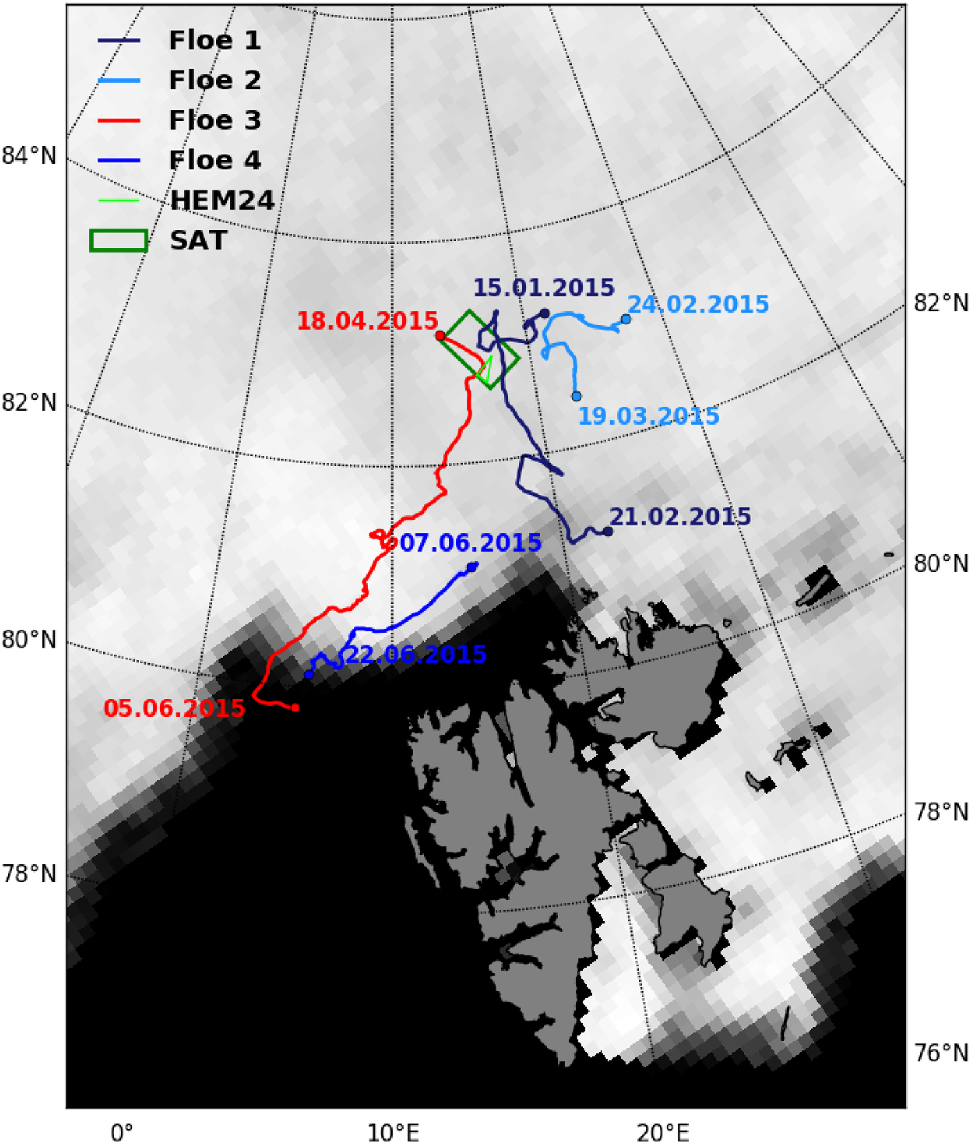
In the following study, we will focus on observations from the N-ICE2015 drift of Floe 3, lasting from 18 April to 5 June 2015 (Granskog and others, Reference Granskog2016); see also Figure 1. The ice station was set up on a floe that included or was close to different ice types: refrozen leads (RL), first year ice (FYI), and second year ice (SYI) with modal total thickness of 0.2 m, 1.2 m, and 2.3 m, respectively (Rösel and others, Reference Rösel2016a). Ice types were identified by salinity and isotope analyses, in combination with sea-ice thickness (Granskog and others, Reference Granskog2017). Snow thickness was on average 0.45 m on FYI and SYI (Rösel and others, Reference Rösel2016b), on the RL it was about 0.02 m, consisting of blowing snow adhering to frost flowers on the surface (Rösel and others, Reference Rösel2016b). A calculated back-trajectory for the ice station shows that the oldest sea ice originated from September 2013 from the northern Laptev Sea and is thus considered to be SYI (Itkin and others, Reference Itkin2017). Likewise, ice core analysis from Granskog and others (Reference Granskog2017), indicate that the sea ice in the area mainly consisted of only FYI and SYI, broken by refrozen leads and pressure ridges.
Drifts of the ice stations (Floe 1–4) during the N-ICE2015 experiment. In this paper, we focus on data from the drift of Floe 3 (red). The green outline indicates the location of the ALOS-2 satellite scene from 23 April 2015 (SAT), and the light green line shows the co-located track of the helicopter-borne electromagnetic thickness measurements from 24 April 2015 (HEM24). The background is sea-ice concentration (black is 0%; white is 100% sea-ice concentration) from 23 April 2015 based on SSM/I data, calculated with ASI algorithm, provided by ICDC, University of Hamburg.
Ground-based datasets
An electromagnetic instrument (EM31) from Geonics Ltd. (Mississauga, Ontario, Canada) was mounted on a sledge and used to survey the total (snow plus sea-ice) thickness of the surrounding ice pack. The total thickness data we use here in this study are from planned long independent surveys, up to 5 km in one direction in a straight line, with aim to cover all occurring sea-ice classes in a representative manner. These long surveys with the ship in the center are referred to in the following as long ground transects, and they provide the maximum information about the spatial variability in the area surrounding the ice station that can be collected by human observers during one day. Altogether nine long ground transects, containing 25 426 independent data points are analyzed in this study (Rösel and others, Reference Rösel2016a). The EM31 measures the received secondary electromagnetic field, reflected by highly conductive seawater (Kovacs and Morey, Reference Kovacs and Morey1991). Conductivity values were calibrated with drill hole measurements (Rösel and King, Reference Rösel and King2017) and postprocessed according to Haas and others (Reference Haas, Gerland, Eicken and Miller1997) to total (snow and ice) thickness. The footprint size of the EM31 ranges from 3 to 5 m (e.g. Haas and others, Reference Haas, Gerland, Eicken and Miller1997), depending on the underlying snow and ice thickness. The accuracy of EM31 measurements is approximately ± 0.1 m on level ice (Haas and others, Reference Haas, Lobach, Hendricks, Rabenstein and Pfaffling2009), with higher uncertainties on rough and deformed ice.
Airborne surveys
Total ice and snow thickness of Floe 3 and its surroundings (up to 70 km) was also measured by a helicopter-borne EM instrument (HEM) (Ferra Dynamics Inc, Mississauga, Ontario, Canada). Between 15 April and 18 May 2015 16 HEM surveys were undertaken. The HEM flights are all performed from the drifting ship as a basis for the flights, that means the ice pack around the ship stays the same while temporal changes are covered (King and others, Reference King, Gerland, Spreen and Bratrein2016). The HEM instrument operates on the same principle as the ground-based EM31, the height above the sea water is calculated from the strength of the reflected electromagnetic field, induced in the conductive seawater. In addition, the height of the instrument above the surface of the ice or snow is determined with a laser altimeter integrated within the EM instrument (Haas and others, Reference Haas, Lobach, Hendricks, Rabenstein and Pfaffling2009). The difference between the two heights corresponds to the total thickness of ice and snow. The HEM instruments used in this study have horizontal co-planer transmitting and receiving coils spaced 2.7 m apart. They operate at a signal frequency of 4 kHz, with a 10 Hz sampling rate, corresponding to measurement point spacing of 3–5 m (Haas and others, Reference Haas, Lobach, Hendricks, Rabenstein and Pfaffling2009; Pfaffhuber and others, Reference Pfaffhuber, Hendricks and Kvistedal2012). The HEM instrument is flown at a height of 15–20 m above the surface and has a footprint of ~40–50 m (Haas and others, Reference Haas, Lobach, Hendricks, Rabenstein and Pfaffling2009). The nominal total thickness accuracy for a single HEM measurement is 0.1 m over level ice, with significantly larger errors and an underestimation of maximum thickness occurring in heavily ridged areas due to footprint smoothing (Haas and others, Reference Haas, Lobach, Hendricks, Rabenstein and Pfaffling2009; Mahoney and others, Reference Mahoney2015). In addition to the the HEM data, a helicopter-mounted GoPro camera (HERO) recorded every 2 s overlapping images of the flight track for visual interpretation of the HEM data.
Satellite images and sea-ice classification
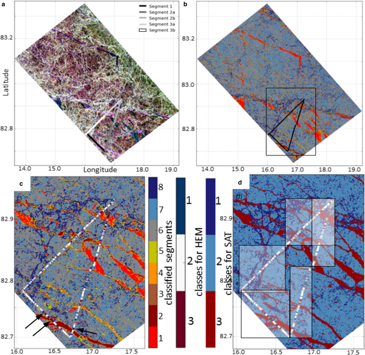
The satellite image used in this study is an ALOS-2 scene from 23 April 2015, 20:18 UTC, provided by Japan Aerospace Exploration Agency (JAXA). The ALOS-2 scene covers an approximate area of 40 km × 70 km, with an azimuth resolution of 3.2 m, a ground range resolution of 5.1 m, and a central incidence angle of 33.9° (Fig. 2a). The processing and analysis of the satellite image has three stages: first, preprocessing and radiometric calibration; second, the application of a segmentation algorithm (Doulgeris and Eltoft, Reference Doulgeris and Eltoft2010; Doulgeris, Reference Doulgeris2013); and third, labeling of the resulting clusters by an ice analyst.
(a) ALOS-2 quad-polarimetric SAR scene, from 23 April 2015, displayed as Pauli image with overlaid co-located HEM track from 24 April 2015 (HEM24). Sections of the HEM24 track used in the statistical analysis are displayed in grayscale. (b) The same scene showed as the clustered image with the HEM track overlaid. The leftmost color-bar shows the eight clusters. For a description and classification of the color-coded clusters see Table 1. The rectangle indicates the subset. (c) Subset of Figure 2b, with overlaid classified HEM24 flight: 1 – ‘thin’ (red), 2 – ‘level’ (white), 3 – ‘deformed’ (dark blue). The arrows indicate the shift between HEM24 data and SAR scene after a first-order drift correction. (d) The eight clusters were combined to three simplified classes: 1 – ‘thin’ (red), 2 – ‘level’ (light blue), and 3 – ‘deformed’ (dark blue). Classified scene is overlaid by classified HEM track. The white-shaded boxes indicate areas used for further statistical comparison of HEM24 track sections with corresponding classified SAR pixels.
Classification results of ALOS-2 scene, acquired on 23 April 2015, shown in Figure 2b
In the preprocessing stage, the satellite scene is radiometrically calibrated using the included metadata calibration information provided by JAXA (Shimada and others, Reference Shimada, Watanabe, Motooka, Kankaku and Suzuki2015) through SNAP (ESA Sentinel Application Platform v2.0.2). Thereafter, a segmentation algorithm, based on feature extraction and segmentation using the ‘extended polarimetric feature space’ (EPFS) method described in Doulgeris and Eltoft (Reference Doulgeris and Eltoft2010) and Doulgeris (Reference Doulgeris2013) is applied. This approach extracts six real-valued features from the original single-look complex SAR image format. For a general-purpose segmentation, we choose a large window size of 27 × 27 pixels and a moderate sensitivity to obtain few and reasonably smooth classes. This smoothing scale (up to 135 m on ground) will segment regional variations rather than the fine scale ice structures, and may result in various degrees of mixed ice type classes, such as low-density ridges in level ice, versus high-density ridging with some level ice, as well as more classical classes like leads or full rubble fields. To reduce the overall processing, we also reduce the image resolution by 3 in each direction, resulting in a image ground resolution of ~10 m × 15 m. The texture feature, or Relative Kurtosis, which measures the non-Gaussianity of the distribution, is calculated from the single-look complex data within the same window as the multi-look averaging. The other five polarimetric features (total scattered power (SPAN), co-polarization ratio, cross-polarization fraction, co-polarization correlation magnitude, and co-polarization correlation phase) are extracted from the multi-look covariance matrix (Doulgeris, Reference Doulgeris2013). The features are non-linearly transformed to improve the spread and symmetry of the clusters. The cluster parameters are then estimated with a traditional expectation maximization (TEM) algorithm, assuming a multivariate Gaussian model for the transformed features. The clustering stage automatically determines the number of clusters using a goodness-of-fit test stage after the TEM-algorithm stage for sequential numbers of clusters (Doulgeris, Reference Doulgeris2013). We choose the lowest number of clusters such that the estimated model is considered a sufficiently good fit to the data, given the chosen sensitivity level. A subsequent contextual smoothing stage, based on a Markov random fields, improves the connectivity of the regions for simpler visual interpretation. The cluster decision is therefore based upon both polarimetric and textural information, and all pixels with similar statistical properties are grouped in the same cluster (Doulgeris, Reference Doulgeris2015). We chose a low sensitivity such that the segmentation stage divided the image into only eight clusters, for subsequent manual identification by ice analysts.
In the final stage, the clusters resulting from the segmentation algorithm were designated following guidelines used by operational ice analysts from the Norwegian Ice Service (NIS), documented by the Canadian Ice Service in the ‘Manual of standard procedures for observing and reporting ice conditions’ (MANICE) (Meteorological Service of Canada, 2005).
The clusters were labeled with a distinct description by an ice analyst (Table 1), and then grouped into three simplified classes: class 1 – ‘thin’, which contains clusters 1–5, class 2 – ‘level’, containing clusters 6 and 7, and class 3 – ‘deformed’, containing cluster 8. To avoid confusion we will continue to refer to the eight clusters (pixels with similar statistical properties grouped together) resulting from the segmentation algorithm as clusters, even when labeled, and use the term ‘class’ only to refer to a simplified class arrived at by grouping together a set of clusters.
The high spatial resolution of the ALOS-2 satellite scenes allows for a good separation between lead and ridging features that have distinct linear patterns but normally differ in brightness, width, and contours which are characteristic to both structures. Leads normally have wide areas of low backscatter between two straight linear features. Low backscatter areas are either open water or new ice formations but can clearly be seen developing in several stages in these large areas between leads. Ridges can either follow a straight trajectory or a slightly winding pattern due to being formed in areas of sea-ice floe convergence. Ridges vary in size where larger ones can have higher brightness and backscatter than smaller ridges where they can be mistaken for hummocked areas. Though they can be distinguished in the segmentation, a certain level of mixing in the single clusters might be present. Areas of smooth FYI are characterized by the rounded dark features in the Pauli image (Fig. 2a). Additional information from the HEM flight (GoPro images combined with thickness information) was used to confirm the decision of the ice analyst.
Drift correction and co-location of the airborne data with satellite information
We make a detailed comparison of the data from a HEM flight that took place on 24 April between 14.27 and 15.30 UTC (named as HEM24 in the following), with the classified ALOS-2 scene, acquired on 23 April, 20.18 UTC. In order to position the HEM24 data relative to the ALOS-2 image, the HEM24 track was relocated to account for the drift of the ice in the intervening time.
Following drift correction the HEM24 track lies completely within the satellite scene (Fig. 2a). The HEM24 track was drift corrected to the reference time of 20.18 UTC, 23 April 2015, using the drift track recorded by RV Lance, under the assumption that the closely packed sea ice has a common mean sea-ice drift for the area. The drift was predominantly in a SSE direction at a rate of approximately 16 km/day. From observations, however, we know that events of high sea-ice dynamics occurred in the study region between 23 and 24 April 2015 (Itkin and others, Reference Itkin2017; Johansson and others, Reference Johansson2017), which leads to a final mismatching especially at the lower part of the image, where open water areas and broken up ice are present. This makes an exact point to pixel alignment very difficult and complex and thus we decided to focus on a regional comparison. We also recognize that the long-time separation between the ALOS-2 scene on 23 April and the HEM24 data acquisition on 24 April could raise concern about the possible introduction of errors into the repositioning of the HEM24 data. But we are not attempting a point to pixel comparison, therefore a more accurate and computationally much more demanding relocation is not necessary.
For our comparison and statistical analysis, we decided to split the HEM24 survey line into five sections: Section 1 is the first part of the flight, the short line of the triangle from west to south east. Section 2a is the first part of the eastern line going northward, section 2b is the second part of the eastern line, sections 3a and 3b are each half of the line from north to southwest (Fig. 2a).
RESULTS
Total snow and ice thickness from in situ measurements
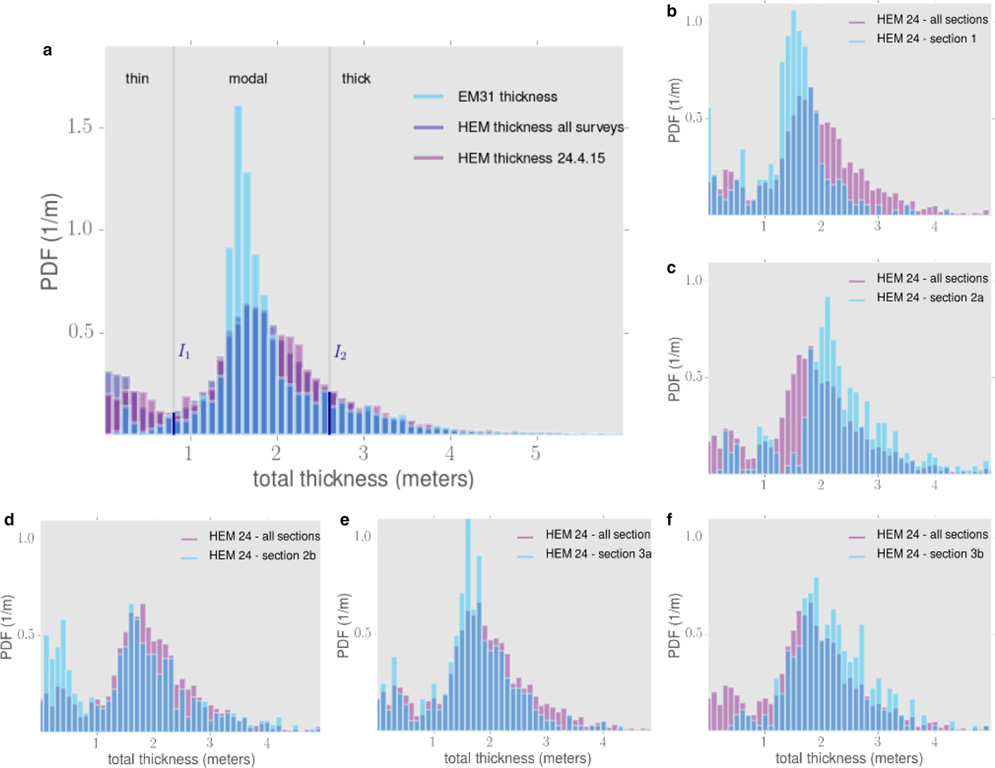
We first present the total snow and ice thickness from EM31 measurements and HEM surveys, referred to as total ice thickness in the following. Figure 3a shows for the total ice thickness, collected with EM31 on long ground transects during April and May on Floe 3, a bimodal probability density function (PDF) with the primary mode at 1.6 m, and a secondary mode at 0.3 m, which represent mainly the level ice and the large refrozen lead in the vicinity of the vessel, respectively (Rösel and others, Reference Rösel2016a). The total ice thickness PDF for all HEM surveys (HEMall) has a mode at 1.7 m and a mean at 1.80 m. There is a second mode between 0.1 and 0.3 m in almost all surveys which represents the refrozen leads (Fig. 3a; King and others, Reference King, Gerland, Spreen and Bratrein2016). The PDF of HEM24 is in good agreement with the PDF of HEMall. The primary mode is at 1.7 m for both, but HEM24 has a second mode at 2.0 m, and a third one at between 0.2 and 0.4 m, matching the mode in the same range in the EM31 distribution (Table 2).
(a) PDFs of total snow and ice thickness of all independent EM31 measurements on Floe 3, all HEM surveys on Floe 3, and the HEM survey on 24 April 2015. I 1 and I 2 are the inflection points at 0.8 and 2.6 m, which distinguish the distribution in three simplified classes: 1 – ‘thin’, 2 – ‘level’, and 3 – ‘deformed’. (b–f) PDFs of the entire HEM24 track compared with the individual sections of HEM24 (defined in Fig. 2).
Mean, modal (secondary modes in brackets), minimum, and maximum sea-ice thicknesses (in meter), and amount of data from electromagnetic instruments (EM31, HEM24, and HEMall)

The similarity between the PDFs of EM31 and HEMall indicates that in this case the EM31 long ground transects are representative of a larger area. The underrepresentation of the thin ice in the EM31 data in favor of an overrepresentation of the level ice is a natural consequence of the way such surveys are carried out (including safety concerns) and should be borne in mind during further discussion or interpretation of the results. It is noticeable that the distribution for the EM31 has steeper slopes than the HEM distributions. Due to the large footprint of the HEM, small, but dominant features like pressure ridges are smoothed and cause a flattening of the slopes in the PDF toward the greater thicknesses.
To define different simplified ice classes within the total ice thickness distribution, we determine threshold points I 1 and I 2 to distinguish between the modal peaks (Hansen and others, Reference Hansen2014). The I 1 is at 0.8 m, defined by the lowest value between the mode at 0.3 m and the primary mode. I 2 is at 2.6 m, defined by the inflection point of the slope of the primary mode toward the deformed ice (Hansen and others, Reference Hansen2014). This slope indicates the transition from level ice to deformed ice, and represents the range where thermodynamic ice growth will be limited. The resulting divisions reflect three simplified ice classes: 1 – ‘thin’: representing predominantly thin ice, 2 – ‘level’: representing predominantly level ice, and 3 – ‘deformed’: representing predominantly thick deformed ice (Fig. 3a).
The calculated fraction for each simplified class is shown in Table 3. The highest fraction is the second simplified class with predominantly level FYI and SYI, which has for EM31, HEMall, and HEM24 80.5, 67.8, and 68.1% of all measurement, respectively. The third simplified class, representing mainly deformed ice, has a fraction of 15.5% for EM31 measurements, and 16.5 and 17.3% for HEMall and HEM24 measurements. The simplified ‘thin’ class shows values of 3.9% (EM31), 15.7% (HEMall), and 14.6% (HEM24).
Fraction of simplified classes in % from different means: EM31, HEMall, HEM24, classified SAT image. Values are rounded. Sections 1 to 3b are described in the text and shown in Figure 2
Table 1 lists the simplified class fractions for each segment defined in Figure 2. These numbers and Figures 3b–f show that the individual HEM24 sections we defined above vary in character. For example, the mode of the simplified class ‘level’ in the sections varies from 1.5 m in section 1 to 2.1 m in section 2. The fractions of the simplified classes ‘thin’ and ‘deformed’ also vary between each section.
Sea-ice classification and total snow and ice thickness
The eight clusters that result from the segmentation of the ALOS-2 image are shown in Figure 2b. The area fraction of each cluster, along with a description derived from analysis of both the segmentation result and the original image, is found in Table 1. Areas of smooth FYI are characterized by the rounded dark features in the Pauli image. Though they can be distinguished in the segmentation (cluster 7), a high level of mixing and some overlapping areas of deformed ice (cluster 6) are also present. The segmentation also separates what appears to be obvious ridging features (cluster 8), particularly in the area that is coincident with the insitu measurements. However, at other places in the image there is confusion between clusters 6 and 8 in places that show from the Pauli image severe roughness from deformed and ridged ice.
As already mentioned above, the eight resulting clusters were merged to three simplified ice classes, intended to be equivalent to the three categories for EM31 and HEM for further comparison: 1 – ‘thin’, which contains clusters 1, 2, 3, 4, and 5, plotted in red; 2 – ‘level’, containing clusters 6 and 7, plotted in light blue; and 3 – ‘deformed’, containing cluster 8, and plotted in dark blue (Fig. 2d). This classified ALOS-2 image is referred to as SAT hereafter. The fractions for the simplified classes in the full scene are 11.2, 74.4, and 14.4%, respectively (Table 3).
We see from the comparison of the flight track with the underlying simplified classes (Fig. 2c), that the thin ice (clusters 1 and 2), as well as the thick, deformed ice or thick level ice with a high surface roughness, i.e. ridges (cluster 8), are captured well by the classification. As already mentioned above, due to the sea-ice drift and deformation, an accurate GPS correction of flight tracks and shifting it over the geo-referenced image is a challenging task and since we applied only a first-order drift correction, a shift is still noticeable, especially in section 1, where high sea-ice dynamic events were observed during the 2 days of data acquisition (Fig. 2c).
To compare HEM24 data with SAT data, we select the SAT pixels from a rectangular subset, underlying the individual HEM24 sections (SAT_sub; see Fig. 2d) and focus on the frequency of occurrence of the simplified classes by displaying them as PDFs or bar plots.
Figures 2b, 3b–f suggest that the sea-ice composition is quite variable: areas with a higher density of thin ice are alternating with those of deformed ice and level ice.
By comparing the three simplified satellite-derived classes to the fraction of simplified classes present in the HEM24 data (Fig. 4, Table 3), we see a spatial variation in the different area fractions for each simplified class. Especially in sections 1, 2a, 3a, and 3b, the differences within one simplified class can be more than 10% and they vary randomly. However, the comparison of the entire HEM24 flight track with the underlaying subset gives a good agreement in all three simplified classes Figure 4g: For simplified class 1 (‘thin’), HEM24 gives 14.6%, while SAT_sub gives 10.5%; the second simplified class (‘level’) has 68.1 and 75.3%, and also the third simplified class (‘deformed’) is well captured with 14.2 and 17.3%, respectively.
Comparison of the area fraction derived from the simplified satellite classes and the frequency of occurrence of the same simplified classes from HEM24 data. (a)–(e) show the direct comparisons of the simplified classes of the five flight sections defined in Figure 2a with their corresponding classified subset areas (Fig. 2d), (f) displays the comparisons of the entire classified HEM24 track with the SAR subset underneath the track (Fig. 2b), and (g) displays the comparisons of the entire classified HEM24 track with the SAR subset and the full SAR scene.
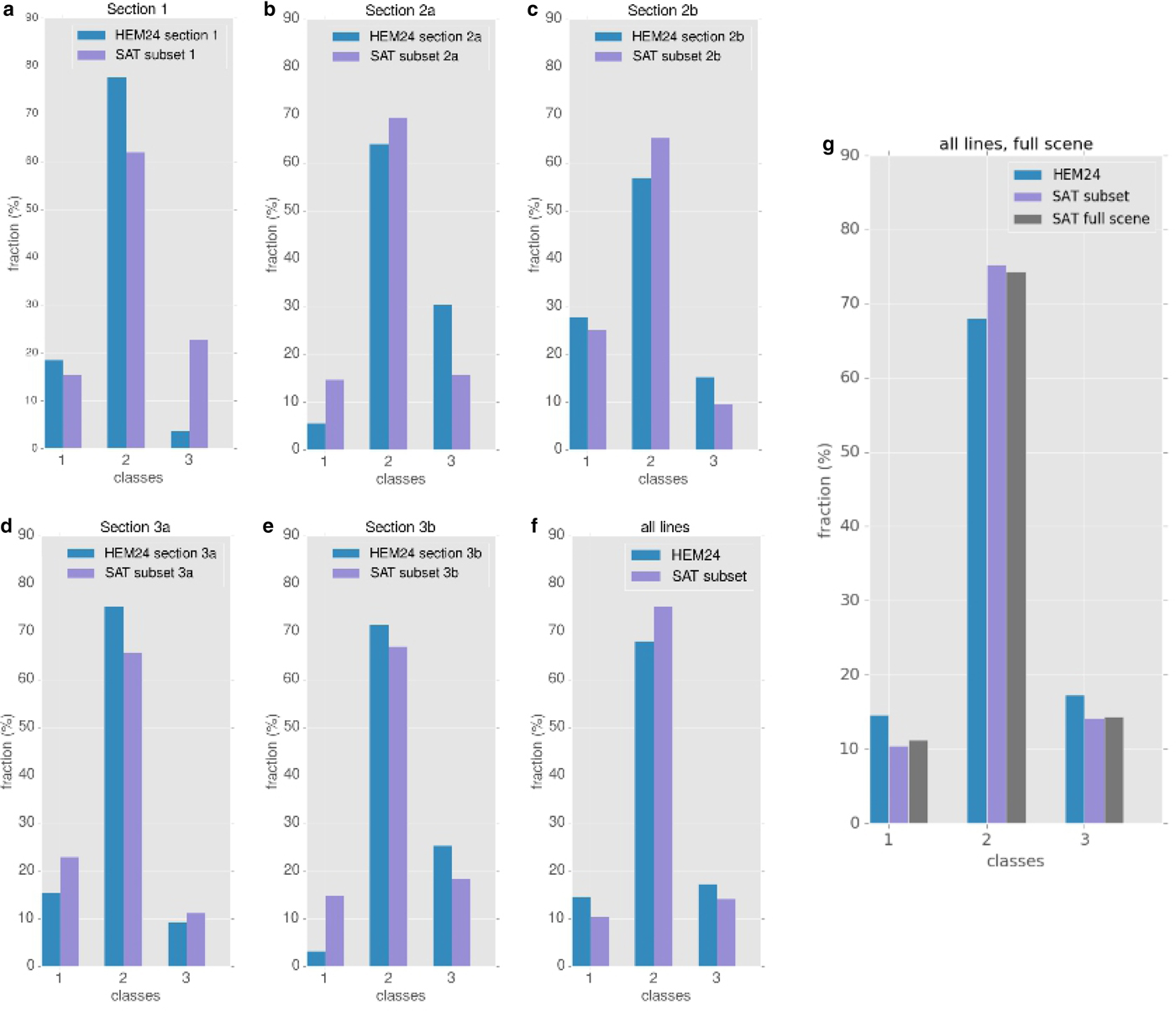
The second simplified class of the analyzed full satellite scene is with 74.4% still in good agreement with the classified SAT_sub and the HEM24 data.
DISCUSSION AND CONCLUSION
In this study, we have analyzed ground- and helicopter-based EM thickness measurements, made in the region north of Svalbard between April and May 2015, to demonstrate the spatial variability of related sea-ice classes, including consolidated ice pack and leads (Table 2). The results have been classified into three simplified classes and compared with a segmented and similarly classified ALOS-2 SAR scene. Returning to the key questions posed in the introduction we can now examine the relationship between the fraction of the three simplified classes at different spatial scales.
We begin with the question of how the ground-based total sea-ice thickness measurements compare to airborne total sea-ice thickness data. The overall comparison of EM31 with HEM24 and HEMall indicates that the ground-based EM31 surveys in our case capture the overall regional ice situation, although the simplified ‘thin’ class is underrepresented and added to the ‘level’ class. Thin ice from the EM31 measurements is present with 4% area fraction compared with 16% (HEMall) and 14% (HEM24), likely because of the natural bias that is caused due the limited access to the refrozen leads and the thinnest ice. The simplified ‘deformed’ class is captured in both methods with 15.5% (EM31) and 17.3% (HEMall), respectively (Table 3). The mode for level ice is, with 1.7 m for HEM and 1.6 m for EM31 comparable in all three EM datasets (Fig. 3). The similarities of the three PDFs (Fig. 3a) demonstrate that long ground transects up to 5 km with ground-based EM31 instruments can give valuable information about the sea-ice conditions, despite covering a smaller area and collecting only a fraction of the data volume when compared with HEMall measurements. The similarity between the PDFs of HEM24 and HEMall also gives us confidence that the flight on the 24 April was over ice that was representative of the ice conditions in the wider region of the campaign (Table 2). But looking at the histograms of the individual sections in Figures 3b–f, 4a–e, we note a significant variation in the abundance of the smaller classes in the range from 3 to 25% and hence very short sections (in the range up to 5–10 km for HEM tracks) might not be representative. To conclude whether the larger track lengths upscale or not, it might be necessary to further investigate the spatial scale of thickness variation within the range of the airborne measurements. In our case, we verified the HEM measurements with the small-scale measurements of the ground-based EM31.
Next, we look at how representative are these local scale measurements of a wider region. Here, the wider region is defined as the area covered by the satellite image. We find that comparing the three simplified classes on the scale of the whole flight, or indeed to all flights carried out in the region during the campaign, gives a satisfying agreement with the simplified class fractions in the whole SAT image. In this example here, the fraction of the ‘thin’ class is 14.5% from the helicopter flight on 24 April 2015, whereas it is 11.2% in the classified satellite scene. The ‘level’ class has 68.1 and 74.4%, respectively, and the ‘deformed’ class gives values of 17.3 and 14.4% (Table 3). Note that this is only the case because the image is roughly uniform. If the chosen subset is moved to different locations within the image, the composition of the simplified classes varies only in the range of ±9%. Both the classified ALOS-2 scene as well as the classified HEM data return a dominant fraction of level ice, combined with a substantial fraction of open water or newly formed and thin ice. Deformed thick ice covers around one-fifth of the area (Table 3). However, once one begins to compare shorter sections of the flight against subsets from the image, this relationship weakens. We are aware that between 23 and 24 April 2015 high winds caused the sea ice to be quite mobile in areas where leads were present. This is most noticeable when section 1 of the HEM is compared with the underlying SAT subset, where the spacing of leads does not match at all. However, the ‘thin’ fraction in this section remains similar between HEM and SAT, indicating that the overall fraction of thin ice and leads within this section did not change even while some significant movement took place.
If we look at the distribution of simplified classes for all lines (Fig. 4 and Table 3), the differences in the area fraction that occur when the comparison is carried out for individual sections, are higher than comparing the sum of the sections to the full underlying subset. This indicates that the specific sea-ice conditions can change over the scale of a kilometer. Hence, it is not recommended to extrapolate such measurements any length beyond their boundary, unless we have further knowledge about the changing sea-ice conditions, such as from the wider view of a satellite image.
Finally, are we able to define regions with similar sea-ice conditions from satellite images? Validation of SAR-based sea-ice classification is an ongoing research topic (e.g. Zakhvatkina and others, Reference Zakhvatkina, Alexandrov, Johannessen, Sandven and Frolov2013; Moen and others, Reference Moen, Anfinsen, Doulgeris, Renner and Gerland2015; Ressel and others, Reference Ressel, Singha, Lehner, Rösel and Spreen2016), which gives scope for improvements. From the along track comparison between HEM and satellite data in Johansson and others (Reference Johansson2017), we can be quite certain of the simplified ‘thin’ class. The separation of the other two classes (‘level’ and ‘deformed’) is less certain, although high and distinct pressure ridges can be identified by their brightness and shape. There is the possibility that pixels can be in the ‘wrong’ class even after the simplification to three classes. The simplified ‘level’ class is very broad and covers a range from 0.8 to 2.6 m of possible thicknesses. The HEM data provide insight into the range of possible thicknesses that could be encountered within this class. It is also possible that old consolidated ridges with limited surface expression are included in the ‘level’ class. It is not possible with the current data and methods to confidentially subdivide this class, and not directly with respect to thickness, thus the SAR data cannot give more detail about the regional distribution of different thicknesses within the ‘level’ class. Our approach is that we are looking at three simplified classes, being aware that these classes might contain mixed ice types, e.g. deformed ice in the ‘level’ class. By this approach, the satellite image scale can provide us information about the distribution of these simplified ice classes at large scales. In addition, the image smoothing (27 × 27 pixels of 3 m × 5 m means a smoothing to the order of 81 m × 135 m) was chosen to focus on larger regional similarities, rather than pixel scale ice types, and thus may also distinguish widespread mixtures.
The findings from this study suggest that satellite data can be used to expand the understanding of sea-ice conditions, in particular the fraction of thin ice and heavily ridged ice with surface expression, in a wider region within which in situ or airborne measurements have been made. This is valuable because widespread in situ measurements represent a logistical challenge and can be very costly. The study also highlights the complexity and limitations of such an approach. One reason for both the good agreement between HEM24 and HEM and the good agreement between the simplified class fractions of HEM24 and the complete image is that this study took place in a region where the composition of the ice pack was similar over a large area. A similar study in a region that happened to encompass, for example, a boundary between a majority FYI region and a majority MYI region might return quite different results. Therefore we suggest to repeat this study for different regions where a different ice situation is present.
In addition, we would like to emphasize that we deliberately decided to use a large window size and a moderate sensitivity for segmentation to obtain few and reasonably smooth clusters, with the limitation of mixed clusters and limitations to distinguish the deformed sea ice and thicker sea-ice types. A future, more detailed, study could build on the work presented here by analyzing whether different levels of spatial averaging result in the identification of different distinct features, and how these are connected to measured sea-ice thickness.
Due to this potential variation at different scales, we recommend that any interpretation of field measurements within a wider context could be supported by satellite image acquisitions, as the satellite image can show where the composition of the ice pack is similar to that of the region in which field measurements took place, and where it is not, at least with respect to SAR detectable properties. This method might also have potential to be applied to SAR wide swath scenes, once the absolute brightness variation relating to the wide incidence angle range is corrected or accounted for in the statistical segmentation algorithm, in order to estimate regions with the similar ice conditions.
ACKNOWLEDGMENTS
The authors acknowledge the efforts of two anonymous reviewers and the scientific editor, Marika Holland. We thank the many scientists that collected an incredible amount of observational data, especially Caixin Wang, Nina Maaß, Martine Espeseth, Marcel Nicolaus, and Chris Polashenski. We also thank the crew and scientists on board R/V Lance, as well as the helicopter pilots from Airlift AS. The authors wish to thank Max König, Marius Bratrein (both NPI) and Thomas Kræmer (UiT) who made the co-located satellite image acquisitions and HEM surveys possible. This work has been supported by the Norwegian Polar Institute's Centre for Ice, Climate and Ecosystems (ICE) through the projects N-ICE2015, SMOSice (ESA; helicopter survey support), ID Arctic (Norw. Ministries of Foreign Affairs; SG, AR), the Norwegian Research Council project (Norw. Ministries of Foreign Affairs and Climate and Environment, programme Arktis 2030) ‘CORESAT’ (NFR project number 222681, JK), the Norwegian Research Council project ‘Centre for Integrated Remote Sensing and Forecasting for Arctic Operations (CIRFA)’ (NFR project number 237906, AD), and the Norwegian Research Council project ‘NORUSS’ (NFR project number 233896, MJ). The ALOS-2 Palsar-2 scene was provided by JAXA under the 4th Research Announcement program (PI: Torbjørn Eltoft). N-ICE2015 acknowledges the in-kind contributions provided by other national and international projects and participating institutions, through personnel, equipment, and other support. Data is available through http://data.npolar.no/.


 Open access