


1. Introduction
Dynamic wetting, the process by which a liquid wets a solid surface, is an important phenomenon that underpins a wide range of both industrial and natural processes, including microfluidics (Stone, Stroock & Ajdari Reference Stone, Stroock and Ajdari2004), liquid coating and printing operations (Weinstein & Ruschak Reference Weinstein and Ruschak2004), petroleum recovery (Gerritsen & Durlofsky Reference Gerritsen and Durlofsky2005), plant protection (Papierowska et al. Reference Papierowska, Szporak-Wasilewska, Szewińska, Szatyłowicz, Debaene and Utratna2018), ground water hydrology (Beatty & Smith Reference Beatty and Smith2010) and biological processes (Barthlott, Mail & Neinhuis Reference Barthlott, Mail and Neinhuis2016). As such, it presents a multiscale problem. Whilst its origin is at the microscopic scale of the moving contact line, it influences outcomes at very much larger scales. However, despite this importance, and consequent research over many decades, there remain fundamental questions about the physics involved and, in particular, the role of solid–liquid interactions at the moving contact line (Andreotti & Snoeijer Reference Andreotti and Snoeijer2020; Afkhami, Gambaryan-Roisman & Pismen Reference Afkhami, Gambaryan-Roisman and Pismen2020; Semenov et al. Reference Semenov, Starov, Velarde and Rubio2011). One such difficulty is the determination of the slip length from experiments. In this paper we develop a continuum model that does not require the slip length, which is difficult to measure experimentally, to be specified. The only parameter that we require is the width of the three-phase zone (TPZ), which can be easily extracted from molecular dynamics (MD) simulations and an experimental determination of the contact line friction for system-specific studies. MD simulations are prohibitively expensive when the physical system size is large, but by simply changing a single parameter in our model we are able to probe the dynamics of larger systems which are beyond the capabilities of MD.
In wetting studies solid–liquid interactions are usually quantified in terms of the angle of contact between the liquid and the solid, and its proper description has attracted much attention (De Gennes Reference De Gennes1985; Blake Reference Blake2006; Shikhmurzaev Reference Shikhmurzaev2007; Andreotti & Snoeijer Reference Andreotti and Snoeijer2020). From hydrostatic and hydrodynamic perspectives, this boundary condition is crucial, as it dictates the shape of the liquid volume. The way it changes in response to movement of the contact line across the solid surface is, therefore, fundamental to our ability to predict wetting outcomes. Nevertheless, the description of the true contact angle at a moving contact line remains hotly debated (Andreotti & Snoeijer Reference Andreotti and Snoeijer2020; Afkhami et al. Reference Afkhami, Gambaryan-Roisman and Pismen2020; Semenov et al. Reference Semenov, Starov, Velarde and Rubio2011).
In continuum models the true contact angle, measured by the tangent of the interface at the solid (see figure 1), has to be specified in order to solve the governing equations and is usually considered to be constant and equal to the equilibrium value. The observed dynamics of the apparent contact angle (i.e. the one seen experimentally Wilson et al. Reference Wilson, Summers, Shikhmurzaev, Clarke and Blake2006) is attributed to the ‘viscous bending’ of the interface: this is the so-called ‘hydrodynamic’ or Cox–Voinov formulation (Cox Reference Cox1986; Voinov Reference Voinov1976). However, according to the molecular-kinetic theory (MKT) of wetting (Blake & Haynes Reference Blake and Haynes1967; Blake Reference Blake1993) and the interface formation model (Shikhmurzaev Reference Shikhmurzaev2007), the true contact angle varies and is dependent on the velocity of the contact line.

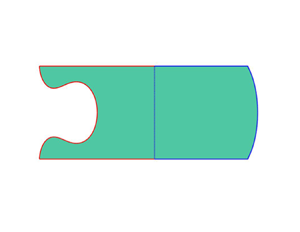
Figure 1. Schematic of a liquid plug between two plates subject to an external forcing  $F^*_0$. The angle that the receding contact line makes with the plate is the true angle, denoted $\theta _{{cl}}$. See figure 6 for a more detailed schematic of the angle measurements.
Here, we will show that viscous bending alone is insufficient to capture the effects seen in molecular simulations, where the velocity dependence of the actual contact angle is observed. Therefore, we develop a new combined approach based on the Navier–Stokes continuum paradigm combined with the MKT (whose formulation is far simpler than the interface formation model, despite the latter's attractive features) and focus it on the canonical dynamic wetting problem of a liquid plug propagating through a channel. In particular, in order to allow for unambiguous comparisons to the results of MD on a comparable system, we identify a critical speed at which a flow bifurcation occurs and a thin film is formed.
The study of dynamic wetting using molecular simulations has a long history, see review articles De Coninck & Blake (Reference De Coninck and Blake2008) and Koplik & Banavar (Reference Koplik and Banavar1995); but here we focus on a recent paper, Fernández-Toledano et al. (Reference Fernández-Toledano, Blake and De Coninck2021), that examines both wetting transitions and the behaviour of the contact angle. In this study large-scale MD is utilised to explore the steady displacement of a water-like liquid plug between two molecularly smooth solid plates under the influence of an external driving force  $F^*_0$ (see figure 1 for the geometry). The study used a coarse-grained model of water and an atomistic Lennard–Jones model for the solid plates. The general behaviour observed as $F^*_0$ was increased and, hence, the liquid plug's speed was raised, is depicted in figure 2. Notably, it was reported that both the ‘true’, dynamic contact angle at the contact line, $\theta _{{cl}}$, and a larger-scale ‘apparent’ angle, $\theta _{{app}}$, are dependent on the contact line velocity $U_{{cl}}^*$ for the receding and advancing interfaces. Henceforth, unless otherwise stated, when we refer to a ‘contact angle’ we mean the ‘true’ contact angle. We also note that quantities labelled with an asterisk correspond to dimensional physical quantities and those without to dimensionless quantities.

Figure 2. Figure reprinted from Fernández-Toledano, Blake & De Coninck (Reference Fernández-Toledano, Blake and De Coninck2021), with permission from Elsevier. Panels (a–e) show the liquid plug as the force  $F^*_0$ (in the article asterisks were not used to denote dimensional quantities) becomes successively larger and eventually exceeds the critical value (panels d,e) where a thin film begins to develop. In this MD simulation the external phase is a vacuum.
In the MD study, the apparent angle was measured at the system scale by a method that mimics typical measurements of it in macroscopic experiments, where the precise details of the true contact angle's dynamics remain hidden, as they occur on such small length scales (Hoffman Reference Hoffman1975; Dussan Reference Dussan1979; Blake Reference Blake2006). By varying the solid–liquid affinity (i.e. the solid's wettability), it was possible to investigate the influence of the equilibrium contact angle  $\theta _0$ on the results. For all $\theta _0$, $\theta _{{cl}}$ was found to be velocity dependent in a manner consistent with the MKT of dynamic wetting (Blake & Haynes Reference Blake and Haynes1967; Blake Reference Blake1993). However, $\theta _{{app}}$ diverged from $\theta _{{cl}}$ as $F^*_0$ was increased, especially at the receding contact line (RCL), in a way that closely followed the Voinov equation (Voinov Reference Voinov1976)
 \begin{equation} \theta_{{app}}^3 = \theta_{{cl}}^3 + 9\,Ca\log(L^*/L_m^*), \end{equation}
where  $Ca=\mu ^* U_{{cl}}^*/\gamma ^*$ is the capillary number based on the contact line speed $U_{{cl}}^*$, dynamic viscosity $\mu ^*$ and surface tension $\gamma ^*$, and $L^*$ and $L_m^*$ are suitably chosen macroscopic and microscopic length scales. For each $\theta _0$, there was a critical RCL velocity $U_{{crit}}^*$ and contact angle $\theta _{{crit}}$ at which $\theta _{{app}}$ became small and the receding meniscus deposited a liquid film on the plates. This value could then be used in (1.1), assuming $\theta _{{app}}\approx 0$, to fix $L^*/L^*_m$ and, hence, reliably predict $\theta _{{cl}}$ at both the ACL and RCL. This result is significant, as $\theta _{{cl}}$ is not usually experimentally accessible and the fact that it varies with $U_{{cl}}^*$ poses questions for hydrodynamic interpretations of dynamic wetting. The result also shows that the critical condition for film deposition encodes crucial information about the hydrodynamics.
The existence of a critical wetting speed has been investigated thoroughly using hydrodynamic models in a range of geometries, including those associated with coating flows (Kumar Reference Kumar2015) and plate withdrawal (Snoeijer et al. Reference Snoeijer, Ziegler, Andreotti, Fermigier and Eggers2008), among others. In Keeler et al. (Reference Keeler, Lockerby, Kumar and Sprittles2021) both receding and advancing contact line (ACL) problems were investigated for a coating flow and the stability of the solutions near the critical speed was quantified using a dynamical systems method. Here, our focus will be on the RCL, as this is where the first bifurcation will occur. Previous studies have shown that as  $Ca$ increases, the RCL will attain a steady state provided $Ca< Ca_{{crit}}$, where $Ca_{{crit}}$ is a critical capillary number that is a function, at the very least, of $\theta _{{cl}}$, the slip length and the viscosity ratio of the liquid and gas phases (Cox Reference Cox1986; Eggers Reference Eggers2004; Snoeijer et al. Reference Snoeijer, Delon, Andreotti and Fermigier2006, Reference Snoeijer, Andreotti, Delon and Fermigier2007; Keeler et al. Reference Keeler, Lockerby, Kumar and Sprittles2021), but, if $Ca>Ca_{{crit}}$, a thin film develops with thickness dependent on $Ca$ (Snoeijer et al. Reference Snoeijer, Delon, Andreotti and Fermigier2006; Keeler et al. Reference Keeler, Lockerby, Kumar and Sprittles2021). Using a lubrication model, $Ca_{{crit}}$ can be approximated when the slip length is small relative to the film height (Eggers Reference Eggers2005), by considering a small- $Ca$ asymptotic analysis and using the key assumption that $\theta _{{app}} = 0$ at the critical point. However, in a nano-geometry, as considered here, we will see that this assumption is not valid and the resulting small- $Ca$ asymptotic analysis does not extend to this regime.
In this paper we will develop a hydrodynamic model based on the Navier–Stokes paradigm to calculate steady states and transient behaviour of the liquid plug scenario considered in Fernández-Toledano et al. (Reference Fernández-Toledano, Blake and De Coninck2021). An essential aspect of this model is that the true angle,  $\theta _{{cl}}$, has to be specified at the junction of the liquid, gas and solid phases. In many previous studies where a Navier–Stokes model is used (see, e.g. Sprittles & Shikhmurzaev Reference Sprittles and Shikhmurzaev2012; Kamal et al. Reference Kamal, Sprittles, Snoeijer and Eggers2019; Liu, Carvalho & Kumar Reference Liu, Carvalho and Kumar2019; Vandre, Carvalho & Kumar Reference Vandre, Carvalho and Kumar2012, Reference Vandre, Carvalho and Kumar2013; Liu et al. Reference Liu, Vandre, Carvalho and Kumar2016a,Reference Liu, Vandre, Carvalho and Kumarb; Liu, Carvalho & Kumar Reference Liu, Carvalho and Kumar2017) $\theta _{{cl}}$ is assumed to be constant and, in others, whilst the angle varies this is to account for sub-grid-scale variations in the apparent angle, rather than variation of $\theta _{{cl}}$ (Sui, Ding & Spelt Reference Sui, Ding and Spelt2014).
Motivated by the results of Fernández-Toledano et al. (Reference Fernández-Toledano, Blake and De Coninck2021) we relax this assumption and adopt a model that determines  $\theta _{{cl}}$ as a function of $Ca$ and the static contact angle $\theta _0$ based on the MKT. Notably, the model remains hydrodynamic throughout, in contrast, for example, to Hadjiconstantinou (Reference Hadjiconstantinou1999), and the molecular augmentation comes entirely through the contact angle formula.
The approach of using molecular simulations to develop a macroscopic framework for dynamic wetting builds on a number of influential works in this area. Notably, in Qian, Wang & Sheng (Reference Qian, Wang and Sheng2003) molecular simulations revealed the existence of the ‘uncompensated Young stress’ in the contact line region that led the authors to derive a ‘generalized Navier boundary condition’ that fits into a Cahn–Hilliard computational framework where the molecular-scale diffuse nature of the interface is resolved. In Ren & E (Reference Ren and Weinan2007) a careful analysis of contact line force contributions in MD was also considered, but within the sharp-interface regime this led the authors to propose a hydrodynamic model similar to the one considered here, Navier slip and the use of the MKT to account for the contact line region's dynamics. This work was extended in Ren, Hu & E (Reference Ren, Hu and Weinan2010) to account for complete wetting states. Again, motivated by MD, more recent approaches have even considered modifications to impermeability of the solid–liquid interface (Lukyanov & Pryer Reference Lukyanov and Pryer2017) that change the flow kinematics near the contact line. Notably, such models subsequently became the basis of macroscopic CFD-type codes for wetting, e.g. Xu & Ren (Reference Xu and Ren2014) and Yue & Feng (Reference Yue and Feng2011). Previous articles considering MD have, understandably, focused on steady states where the advantages of time averaging of MD obtained quantities can be exploited. Here, we expand on these articles to focus on flow instabilities at the RCL, which is known to be a sensitive test for dynamic wetting theories (Snoeijer & Andreotti Reference Snoeijer and Andreotti2013).
Macroscopic models previously proposed, including, in particular, those using the MKT (Reddy, Schunk & Bonnecaze Reference Reddy, Schunk and Bonnecaze2005; Dodds, Carvalho & Kumar Reference Dodds, Carvalho and Kumar2012), often consider that the static contact angle,  $\theta _0$, and slip length are independent parameters. Motivated again by Blake et al. (Reference Blake, Fernández Toledano, Doyen and De Coninck2015) and Fernández-Toledano, Blake & De Coninck (Reference Fernández-Toledano, Blake and De Coninck2020b), we will make use of a correlation between slip length and $\theta _0$ that reduces the number of parameters that are required. This correlation is based on an assumption, borne out by MD simulations, that the mechanism of slip between a liquid and a solid is the same across all parts of the solid–liquid interface, including the contact line.
The paper is structured as follows. In § 2 we describe the system of equations used to model the liquid plug based on the Navier–Stokes equations. In addition to the Navier–Stokes equations, in § 3 we discuss asymptotic results, based on a quasi-parallel (QP) lubrication approach adapted from Eggers (Reference Eggers2005), that will be relevant here. By calculating numerical solutions of the governing equations using a finite-element framework, we will then show in § 4 that the critical speed of wetting for the entire liquid plug is dependent on the RCL and not influenced by the ACL. We will also discuss the method for calculating the apparent angle. Next, in § 5 we will show how augmenting the Navier–Stokes equations with an MKT variable-angle (VA) constraint predicts the existence of a critical  $Ca$, and that as the wettability is varied the values of $Ca_{{crit}}$ match favourably with the MD data in Fernández-Toledano et al. (Reference Fernández-Toledano, Blake and De Coninck2021), in contrast to the predictions of the fixed-angle model. In addition, we demonstrate how $\theta _{{cl}}$ and $\theta _{{app}}$ vary with the slip length and, thus, provide an estimate of $L^*/L_m^*$ for the liquid plug system, which shows excellent agreement with the MD simulations. Furthermore, in § 6 we examine time-dependent behaviour when $Ca>Ca_{{crit}}$ so that a thin film develops, whose height obeys a Landau–Levich law. Finally, in § 7, having validated the system in the liquid nano-plug geometry, we exploit our computational framework to explore larger-scale systems, which are beyond the scope of MD simulations. By examining systems where the physical size is orders of magnitude larger than the nano-channel studied in Fernández-Toledano et al. (Reference Fernández-Toledano, Blake and De Coninck2021), we will show that the dimensionless thickness of the film remains constant for a fixed $Ca$.
$Ca$.
2. Molecular-augmented hydrodynamic model
We will now describe the hydrodynamic model. We shall discuss the full system, based on the Navier–Stokes equations and then describe two different system formulations, the pressure-driven problem and the force-driven problem, as well as the numerical method and the different computational domains.
2.1. Fully nonlinear system
To mimic the molecular simulations, we model the liquid-bridge system as a two-dimensional flow between two parallel plates as illustrated in figure 1 and detailed in figure 3(a). A finite liquid region fills the channel bounded by two rigid plates that are separated by a distance  $H^*$. We solve in a frame of reference that moves with the plug, with the walls moving with velocity $U_{{wall}}^*$. The exact formulation depends on the domain and problem that we consider (i.e. pressure-driven or body-force driven), details of which we discuss later. We non-dimensionalise all lengths using the half-height, $H^*/2$, all velocities using $U_{{wall}}^*$, all pressures by $\mu ^* U_{{wall}}^*/(H^*/2)$, all time scales by $(H^*/2)/U_{{wall}}^*$ and the body force by $\mu ^* U_{{wall}}^*/(H^*/2)^2$. The physical values from the nano-channel geometry of Fernández-Toledano et al. (Reference Fernández-Toledano, Blake and De Coninck2021) are $H^* = 20.2\ \mbox {nm}$, $\mu ^* = 0.37\ \mbox {mPa}\ \mbox {s}^{-1}$, $\rho ^* = 997\ \mbox {kg}\ \mbox {m}^{-3}$ and $\gamma ^* = 66\times 10^{-3}\ \mbox {N} \mbox {m}^{-1}$. The physical velocity $U_{{wall}}^*$ ranges from $1\ {\rm to}\ 10^2\ \mbox {m}\ \mbox {s}^{-1}$. As in other studies (Sprittles & Shikhmurzaev Reference Sprittles and Shikhmurzaev2011b,Reference Sprittles and Shikhmurzaeva; Vandre et al. Reference Vandre, Carvalho and Kumar2012; Sprittles & Shikhmurzaev Reference Sprittles and Shikhmurzaev2013; Vandre et al. Reference Vandre, Carvalho and Kumar2013; Liu et al. Reference Liu, Vandre, Carvalho and Kumar2016a,Reference Liu, Vandre, Carvalho and Kumarb, Reference Liu, Carvalho and Kumar2017, Reference Liu, Carvalho and Kumar2019), we apply the Stokes-flow approximation, (2.1)–(2.2), so that the Reynolds number, $\rho ^*U_{{wall}}^*H^*/\mu ^*$, is assumed to be negligibly small; simple estimates confirm that this is appropriate for the nano-system. We neglect the influence of gravity and assume that the gas phase can be modelled as a vacuum (as seen in figure 2, there are no molecules in the gas phase). A typical computational domain is shown in figure 3(a). On the moving wall ( $y=0$) we apply a Navier-slip condition, (2.3), and, therefore, introduce a dimensionless slip length, $\lambda$. The MD simulations in figure 2 indicate the flow is symmetric around the centreline of the channel and, hence, we introduce a symmetry wall at $y=1$, labelled $\varGamma _2$, where we set the vertical component of velocity to be zero, apply zero tangential stress and let the horizontal velocity be determined as part of the solution. As well as the fluid velocity field, ${\boldsymbol {u}}(t,{\boldsymbol {x}})$, and pressure, $p(t,{\boldsymbol {x}})$, which depend on the dimensionless time, $t$, and the position, ${\boldsymbol {x}}$ of the interfaces, denoted ${\boldsymbol {R}}_{{adv}}=(x_{a}(t,s),y_{a}(t,s))$ and ${\boldsymbol {R}}_{{rec}}=(x_{r}(t,s),y_{r}(t,s))$, respectively, are also unknowns in the problem and functions of $t$ and the arclength, $s$, as measured from the contact point. These are found using dynamic and kinematic conditions on both free surfaces. The governing equations and boundary conditions then become
 \begin{gather} 0={-}\boldsymbol{\nabla} p + \nabla^2{\boldsymbol{u}} + {\boldsymbol{F}}, \quad{\boldsymbol{x}}\in\varOmega, \quad\mbox{Conservation of momentum}, \end{gather}
 \begin{gather}\boldsymbol{\nabla}\boldsymbol{\cdot}{\boldsymbol{u}} = 0,\quad{\boldsymbol{x}}\in\varOmega,\quad \mbox{Incompressibility}, \end{gather}
 \begin{gather}\lambda (\boldsymbol{\tau} \boldsymbol{\cdot} {\boldsymbol{n}})\boldsymbol{\cdot}{\boldsymbol{t}}, = ({\boldsymbol{u}} - {\boldsymbol{U}})\boldsymbol{\cdot} {\boldsymbol{t}},\quad{\boldsymbol{x}}\in \varGamma_{4},\quad \mbox{Navier-slip condition}, \end{gather}
 \begin{gather}{\boldsymbol{u}}\boldsymbol{\cdot}{\boldsymbol{n}} =0, \quad{\boldsymbol{x}}\in\varGamma_{4}, \quad\mbox{No-penetration condition}, \end{gather}
 \begin{gather}{\boldsymbol{u}}\boldsymbol{\cdot}{\boldsymbol{n}} =0, (\boldsymbol{\tau}\boldsymbol{\cdot}{\boldsymbol{n}})\boldsymbol{\cdot} {\boldsymbol{t}} =0, \quad{\boldsymbol{x}}\in\varGamma_{2},\quad \mbox{Symmetry condition}, \end{gather}
 \begin{gather}\boldsymbol{\tau}\boldsymbol{\cdot}{\boldsymbol{n}} = \frac{1}{Ca}\kappa {\boldsymbol{n}},\quad{\boldsymbol{x}}\in\varGamma_{1}\cup\varGamma_{3},\quad \mbox{Dynamic condition (receding & advancing)}, \end{gather}
 \begin{gather}\frac{\partial {\boldsymbol{R}}_{{adv}}}{\partial t}\boldsymbol{\cdot}{\boldsymbol{n}} = {\boldsymbol{u}}\boldsymbol{\cdot}{\boldsymbol{n}},\quad {\boldsymbol{x}}\in\varGamma_{1},\quad \mbox{Kinematic condition (advancing)}, \end{gather}
 \begin{gather}\frac{\partial {\boldsymbol{R}}_{{rec}}}{\partial t}\boldsymbol{\cdot}{\boldsymbol{n}} = {\boldsymbol{u}}\boldsymbol{\cdot}{\boldsymbol{n}},\quad{\boldsymbol{x}}\in\varGamma_{3},\quad \mbox{Kinematic condition (receding)}, \end{gather}
where  ${\boldsymbol {n}}$ and ${\boldsymbol {t}}$ are the vectors normal and tangential, respectively, to the appropriate boundaries denoted $\varGamma _i$, and $\kappa$ is the curvature of the corresponding interface. The plate speed ${\boldsymbol {U}} = (U_{{wall}},0)^{\rm T}$ and $\lambda = \lambda ^*/(H^*/2)$ is the dimensionless slip length. The body force is ${\boldsymbol {F}} = (F,0)^{\rm T}$, where $F$ is a set constant. The stress tensor $\boldsymbol {\tau }$ is defined as
 \begin{equation} \boldsymbol{\tau} ={-}p{\boldsymbol{\mathsf{I}}} + \left(\boldsymbol{\nabla} {\boldsymbol{u}} + (\boldsymbol{\nabla}{\boldsymbol{u}})^{\rm T}\right), \end{equation}
where  ${\boldsymbol{\mathsf{I}}}$ is the identity matrix. We shall refer to the system described by (2.1)–(2.8) as the ‘half-liquid plug’ problem.

Figure 3. The computational domain with streamlines and computational elements in the background. (a) Half-liquid plug domain – the upper boundary,  $\varGamma _2$ is a symmetry boundary and $\varGamma _4$ is a moving wall, so we are computing the system in a frame of reference that moves with the liquid. (b) Receding contact line domain where, instead of a free surface at $\varGamma _1$, we impose parallel flow which significantly reduces the computational burden. (c) Advancing contact line domain. In (b,c) the circular markers on the free surfaces indicate the location of the inflection point, denoted IP. Parameter values are $Ca = Ca_{{crit}} = 0.31$, $\lambda = 0.1$, $\theta _{{cl}} = {\rm \pi}/2$.
2.2. Contact angle models
The system is not well-posed unless a contact angle is specified between the free surfaces and the horizontal plates. For the symmetry boundary, we set  $\theta (s = L) = {\rm \pi}/2$, but the dynamic contact angle, $\theta _{{cl}}$, can be freely chosen and depends on the wettability of the solid.
The simplest approach is to specify a constant equilibrium contact angle, i.e.
 \begin{equation} \theta_{{cl}} = \mbox{const.},\quad \mbox{Constant angle equation}.\end{equation}
However, as is well known, the MKT predicts  $\theta _{{cl}}$ to be dependent on the speed of the contact line. As shown in Appendix A, for the RCLs of interest here, this dependence may be written in the linearised form
 \begin{equation} \overline{Ca} =\frac{\lambda}{\delta}\left(\cos(\theta_0) - \cos(\theta_{{cl}})\right),\quad \mbox{VA equation}, \end{equation}
where  $\delta$ is a dimensionless parameter that corresponds to the width of the TPZ, i.e. the contact line viewed at the molecular scale, and $\overline {Ca}$ is the relative velocity of the contact line to the wall speed, i.e.
 \begin{equation} \overline{Ca} = Ca\left({\boldsymbol{U}}\boldsymbol{\cdot} {\boldsymbol{e}}_x - \left.\frac{\partial x}{\partial t}\right|_{s = 0}\right), \end{equation}
where  ${\boldsymbol {e}}_x$ is a unit vector in the $x$ direction. Equation (2.11) is the linearised form of the theory, which will be valid for the system considered in this article. Furthermore, it has long been recognised that a relationship must exist between the slip length and the equilibrium contact angle, e.g. Tolstoi (Reference Tolstoi1952), Barrat & Bocquet (Reference Barrat and Bocquet1999) and Priezjev (Reference Priezjev2007). Here, motivated by the results of Fernández-Toledano et al. (Reference Fernández-Toledano, Blake and De Coninck2021) and the theory described in Appendix A, we consider the relationship
 \begin{equation} \lambda_{{MD}}^* = a\exp\left[b(1 + \cos(\theta_0)\right],\quad 0<\theta_0<{\rm \pi}, \end{equation}
where  $a$ and $b$ are fitting parameters and $\lambda _{{MD}}^*$ is the physical slip length derived from the MD data in Fernández-Toledano et al. (Reference Fernández-Toledano, Blake and De Coninck2021). We will assume that $\lambda _{{MD}}^*$ is independent of the physical channel height, $H^*$, and, therefore, in our non-dimensionalisation $\lambda = 2\lambda _{{MD}}^*/H^*$. To investigate the nano-channel used in Fernández-Toledano et al. (Reference Fernández-Toledano, Blake and De Coninck2021), where $H^* = 20.2\ \mbox {nm}$, the different values of $\theta _0$ will yield dimensionless slip lengths in the range $\lambda \sim 0.02$ to $0.2$. Alternatively, as we will show in § 7, by varying $\lambda$, and keeping $\theta _0$ fixed, we can investigate the effects of varying the physical channel height $H^*$ to larger systems. We emphasise that there is a one-to-one correspondence between $\lambda _{{MD}}^*$ and $\theta _0$, and hence, we are free to prescribe either quantity and use (2.13) to determine the other. In physical experiments it is more practical to find $\theta _0$, which can readily be measured, and then determine $\lambda _{{MD}}^*$, which is more difficult to measure experimentally. Figure 4 shows the fit of this function to the MD data from Fernández-Toledano et al. (Reference Fernández-Toledano, Blake and De Coninck2021). We call the system of equations described in (2.1)–(2.8) augmented with the constant angle formula, (2.10), the constant angle (CA) model, while when augmented with the VA formula, (2.11) and (2.13), we call it the VA model.

Figure 4. The slip length dependence on the static angle. The markers are the MD data obtained from Fernández-Toledano et al. (Reference Fernández-Toledano, Blake and De Coninck2021) and the solid line is the curve fit given from (2.13) with  $b = -2.342$ and $a = 5.656\times 10^{-9}$.
2.3. Pressure-driven and force-driven problems
We now discuss the two different types of problems, i.e. the pressure-driven and force-driven problems. The MD simulations in Fernández-Toledano et al. (Reference Fernández-Toledano, Blake and De Coninck2021) is a force-driven problem, but pressure-driven problems are relevant in many practical situations, for example, coating flows (Liu et al. Reference Liu, Carvalho and Kumar2019).
In Pouseille flow, without a free surface, it is easy to show that a pressure-driven problem can be equivalent to a force-driven one. With a free surface however, this is not true and each case has to be considered separately. For steady calculations, in both types of problems, the set of equations are ill-posed unless we specify the volume of the liquid plug. To remove this issue, for pressure-driven flow, we impose a normal stress on  $\varGamma _1$,
 \begin{equation} \boldsymbol{\tau}\boldsymbol{\cdot}{\boldsymbol{n}} = p_{{out}}{\boldsymbol{n}},\quad{\boldsymbol{x}}\in\varGamma_1, \end{equation}
and let the value of  $p_{{out}}$ be determined implicitly by a condition on the overall volume of the liquid plug, which corresponds to the computational area of the domain. We set $F=0$ and solve in a frame of reference that moves such that the walls are non-stationary in the translating frame ( $U_{{wall}} = -1$).
In contrast, for the steady force-driven problem, we set  $U_{{wall}} = -1$ and $p_{{out}} = 0$, but now let $Ca$ be determined implicitly by a volume constraint. In both cases, to overcome the translational invariance, we also have to pin a point on the boundary that depends on the domain of the problem (as discussed below).
For time-dependent problems, whether pressure driven or force driven, the volume constraint is unnecessary, as (2.2) ensures that volume is conserved. Instead, we impose a position constraint for the reduced domains (see below) that determines  $p_{{out}}$ or $Ca$, depending on the problem.
2.4. Numerical method
The complete system of equations are discretised and solved using a finite-element method and the open-source oomph-lib package (Heil & Hazel Reference Heil and Hazel2006), as described in Keeler et al. (Reference Keeler, Lockerby, Kumar and Sprittles2021). An unstructured triangular mesh is used that is treated as a pseudo-elastic body, so that changes to the unknown free surface can be facilitated and the mesh can adapt to capture regions of high velocity or pressure gradients, for example, near the contact point. We use a Zienkiewicz–Zhu (ZZ) error estimator, which measures the continuity of the rate of strain in each element, to identify elements that require refinement or unrefinement (Zienkiewicz & Zhu Reference Zienkiewicz and Zhu1992). As a typical example, for the time-dependent calculations, with  $Ca =0.5$ and $\lambda = 0.01$, elemental areas range from ${\sim }10^{-3}\ {\rm to}\ 10^{-1}$ to accommodate a maximum ZZ error of $10^{-3}$.
2.5. ‘Half’ and ‘quarter’ domains
We can simplify the complexity of the half-liquid plug domain further by solving in two separate ‘quarter’ domains, each having only one free surface; thus, significantly reducing the number of triangular elements required, see figures 3(b) and 3(c). To facilitate this, we replace the free surface (and corresponding dynamic and kinematic boundary conditions) at one end of the computational domain ( $\varGamma _1$ for the ACL and $\varGamma _3$ for the RCL) with an imposed normal stress (i.e. (2.14)) and parallel-flow condition
 \begin{equation} v = 0,\quad{\boldsymbol{x}}\in\varGamma_1\,\, (\mbox{Receding})\quad \mbox{or} \quad {\boldsymbol{x}}\in \varGamma_3\,\, (\mbox{Advancing}). \end{equation}
In these quarter domains, the imposed pressure,  $p_{{out}}$, is determined implicitly by ensuring the volume per unit length (i.e. the area) of the liquid domain is constant (as in the half-liquid plug domain), so that in each quarter domain we are solving in a frame of reference with a fixed volume. We note that in the quarter domains we impose (2.14) and (2.15) in both steady and time-dependent calculations. These quarter domain simulations will be referred to as the ‘receding contact line’ and ‘advancing contact line’ domains (see figure 3b,c), respectively. abbreviated to RCL and ACL in the rest of the paper. The origin is different in each of these domains and corresponds to the pinned position of the steady and time-dependent problems. To illustrate the benefit of this reduction, the number of elements required in the computation of figure 5 for the half-liquid plug is ${\sim }4000\unicode{x2013}8000$, but the number for the RCL is ${\sim }400$. The reason for the $\sim$90 % reduction in elements is because the pressure gradients are not as severe near the RCL, compared with the ACL. In the next section we shall show that the dynamics of the whole system and the prediction of a critical $Ca$ are dominated by the RCL. Thus, computation of the full half-liquid plug problem, where both the advancing and receding interface are calculated, is not necessary in order to find the first flow bifurcation and is computationally inefficient when compared with the reduced RCL domain.

Figure 5. The steady solution space mapped in the  $(Ca,X)$ plane when $\theta _{{cl}} = \mbox {const.} = {\rm \pi}/2$. Here $X_{{adv}}$ and $X_{{rec}}$ are the horizontal distances of the interface at the two plates for the advancing and receding cases, respectively. The solid curves represent the half-liquid bridge problem, while the broken lines indicate the ‘quarter’ problems where the advancing and RCL are calculated separately. The limit point for the RCL indicates the threshold beyond which no steady states exist, denoted by $Ca_{{crit}}$, and corresponds to the critical $F^*_0$ in the MD simulations of Fernández-Toledano et al. (Reference Fernández-Toledano, Blake and De Coninck2021). The inset diagrams correspond to the parameter values $Ca = Ca_{{crit}} \approx 0.31$, $\lambda = 0.2$.
We emphasise that the main aim of this study is to investigate the VA model, and not to make a thorough investigation of the differences between pressure-driven and force-driven flow, as the VA model can be applied independently of the problem. Thus, in the results that follow, we mainly consider pressure-driven flow, except when we make a direct comparison with the MD simulations. For the latter, we present force-driven results, as clearly specified. In addition, as we shall show in § 4.1, the choice of domain is also independent of the problem (i.e. pressure driven or force driven), so we choose the domain that is most important to the flow bifurcation and that is also the simplest, computationally.
3. Reduced governing equations (QP system)
We shall now discuss a reduced evolution partial differential equation model, the so-called QP system, before finally obtaining asymptotic results that will help predict the value of  $Ca_{{crit}}$.
For the RCL, the flow near the contact line is approximately parallel, cf. figure 12, and we can exploit this to reduce the Navier–Stokes equations to a simpler system that requires unknowns only on the fluid interface. As well as the parallel-flow assumption, we assume the horizontal coordinate is approximately the arclength, i.e.  $x\approx s$, so the full expression for the curvature can be used, not the linearized form as used in conventional lubrication models (see, e.g. Eggers Reference Eggers2005) and long-wave models (see, e.g. Snoeijer Reference Snoeijer2006).
Following Jacqmin (Reference Jacqmin2004), Sbragaglia, Sugiyama & Biferale (Reference Sbragaglia, Sugiyama and Biferale2008) and Vandre (Reference Vandre2013), we let  $\theta$ be the angle the interface makes to the horizontal (see figure 1), $h=y_r(s)$ be the height of the interface and $s$ be the arclength coordinate measured from the contact line. Using conservation of mass and the kinematic condition on the free surface, the governing equation for the fluid pressure gradient, ${\partial p}/{\partial s}$, may be written as (Snoeijer et al. Reference Snoeijer, Delon, Andreotti and Fermigier2006)
 \begin{equation} \frac{\partial h}{\partial t} + \frac{\partial Q}{\partial s} = 0,\quad Q = \frac{\partial }{\partial s}\left(-\frac{1}{3}\frac{\partial p}{\partial s}h^2(h + 3\lambda) - ({\boldsymbol{U}}\boldsymbol{\cdot}{\boldsymbol{e}}_x)h\right), \end{equation}
where  ${\boldsymbol {U}}\boldsymbol {\cdot}{\boldsymbol {e}}_x = -1$ for the RCL. The unknown pressure gradient, $\partial p/\partial s$, can then be expressed in terms of the exact curvature by differentiating the normal stress balance with respect to $s$, i.e.
 \begin{equation} \frac{1}{Ca}\frac{\partial^{2} \theta}{\partial s^{2}} = \frac{\partial p}{\partial s}. \end{equation}
In order to solve (3.2), we require two conditions on  $\theta$. At the contact line, $s=0$, we implement (2.11)
 \begin{equation} \overline{Ca} = \frac{\lambda}{\delta}\left(\cos(\theta_0) - \cos(\theta_{{cl}})\right), \end{equation}
and at the symmetry wall,  $s=L$, we set $\theta = {\rm \pi}/2$, where $L$ is the overall length of the interface. The shape of the interface can then be recovered by solving
 \begin{equation} \frac{\partial x}{\partial s} = \cos(\theta),\quad \frac{\partial h}{\partial s} = \sin(\theta). \end{equation}
Each of these equations requires a single condition, so we set  $x(s=0) = y(s=0) = 0$ (choosing the contact line to be at the origin). Finally, we note that the length of the interface, $L$, and, hence, the size of the domain, $s$, are not known a priori. To determine $L$, we scale the independent variable $s$, so that $\xi = Ls$ and $\xi = [0,1]$. The total length of the interface, $L$, can then be determined by the additional constraint that
 \begin{equation} y(\xi = 1) = 1. \end{equation}
To solve this system of equations, we choose to discretise the spatial derivatives using finite differences and then the system of equations are solved numerically using Newton's method. We remark that we exclusively concentrate on the steady results of the pressure-driven QP system and do not solve the time-dependent problem, as this is better suited to the full nonlinear system.
3.1. Asymptotics
We now briefly describe and adapt the analysis of Chan, Snoeijer & Eggers (Reference Chan, Snoeijer and Eggers2012) and Eggers (Reference Eggers2005) to find an asymptotic expression for  $Ca_{{crit}}$. We will not repeat their analysis except for the parts where it differs from the situation we examine here. In both of these previous works gravitational effects are included and the liquid domain is unconfined, whereas we neglect gravity and the system is confined. They also considered only steady solutions, so that time derivatives in the problem can be ignored.
The matched asymptotics methodology of Chan et al. (Reference Chan, Snoeijer and Eggers2012) and Eggers (Reference Eggers2005) is to determine an inner solution, say  $h = h_{{inner}}$, for small $Ca$, that is valid close to the contact line, i.e. when $s/\lambda \sim {O}(1)$, and an outer solution, $h = h_{{outer}}$ say, that is valid far away from the contact line, i.e. when $s\sim {O}(1)$. To determine an unknown constant in the outer solution, the inner and outer solutions have to match in a crossover region. This matching procedure yields an equation, for an arbitrary unknown, $\theta _{{app}}$, which is the angle the outer interface makes with the horizontal. For the ACL domain, $\theta _{{app}}$ is finite for all values of $Ca$, and thus, in these asymptotic limits at least, there is no critical point for the ACL domain. However, in the RCL domain $\theta _{{app}}$ can only be calculated up to a critical value of $Ca$, this value being interpreted as $Ca_{{crit}}$.
In our problem, for a confined geometry and in the absence of gravity, the inner region analysis near the contact line is identical to the case considered in Chan et al. (Reference Chan, Snoeijer and Eggers2012) and Eggers (Reference Eggers2005). In Eggers (Reference Eggers2005) the effects of gravity are present at first order in the outer solution. The outer solution, for small  $Ca$, is found by expanding the unknowns as a power series in $Ca$. We can write a leading-order outer solution of (3.1a,b) to (3.4a,b) as
 \begin{equation} \left.\begin{gathered} \theta_{{outer}} = \theta_{{app}} + \kappa_s s, \quad h_{{outer}} = 1-\frac{1}{\kappa_s}\cos \left(\theta_{{app}} + \kappa_s s\right),\\ x_{{outer}} = \frac{1}{\kappa_s}\left[\sin\left(\theta_{{app}} + \kappa_s s\right) - 1\right] + X_{{rec}}, \end{gathered}\right\}\end{equation}
where  $\kappa _s = ({\rm \pi} - 2\theta _{{app}})/2L$ is the curvature, $X_{{rec}}$ is the meniscus rise (cf. figure 5) and $\theta _{{app}}$ is an undetermined constant. The outer solution in (3.6) describes a sector of a circle with centre $(X_{{rec}} - r,1)$ and $r = 1/\kappa _s$ that makes an angle $\theta _{{app}}$ to the horizontal at $s=0$. Examining the geometry (see dashed curve in figure 6a) gives $\kappa _s = \sin ({\rm \pi} /2 - \theta _{{app}}),$ so as $\theta _{{app}}\to 0$, $\kappa _s\to 1$ and, hence, the interface is a semi-circle of radius 1. In particular, we have
 \begin{equation} L\to {\rm \pi}/2,\quad X_{{rec}}\to 1,\quad\mbox{as}\ \theta_{{app}}\to 0. \end{equation}
When the outer solution, described in (3.6), is matched to the inner solution, as described in Eggers (Reference Eggers2005), we obtain an expression for  $\theta _{{app}}$,
 \begin{equation} \frac{\theta_{{app}}}{\theta_{{cl}}^3} ={-}\frac{2^{2/3}3^{1/3}Ca^{1/3}\mathrm{Ai}'(z_1)}{\mathrm{Ai}(z_1)}, \end{equation}
where  $\mathrm {Ai}(z)$ is an Airy function of the first kind. We note this is the same for an unconfined geometry with gravity as considered in Eggers (Reference Eggers2005). In addition, $Ca_{{crit}}$ satisfies the same expression as in Eggers (Reference Eggers2005) but has a factor of $2^{1/3}$ in the denominator of the logarithm term, i.e.
 \begin{equation} Ca_{{crit}} = \frac{\theta_{{cl}}^3}{9}\left[\log\left(\frac{Ca_{{crit}}^{1/3}\theta_{{cl}}}{3^{2/3} \boldsymbol{\cdot} 2^{1/3}\mathrm{Ai}^2(z_{{max}})\lambda{\rm \pi}}\right)\right]^{{-}1},\quad z_{{max}} ={-}1.0188. \end{equation}
The difference between (3.9a,b) and the equivalent expression in Eggers (Reference Eggers2005) is down to the far-field boundary conditions; in our problem the fluid is confined, and in Eggers (Reference Eggers2005) it extends to infinity. These results are valid for a constant contact angle model but we can easily extend them to our VA formula by expanding (2.11) in powers of  $Ca$, for $Ca\ll 1$, and then $\theta _{{cl}}$ in the above expression is just the static angle $\theta _{0}$. However, we will show that the full expression for $\theta _{{cl}}$ in (2.11) will be required in the formula (3.9a,b) for it to compare favourably with the numerical results. In the sections that follow, the expressions in (3.7), (3.8) and (3.9a,b) will be compared with the numerical solutions.

Figure 6. The alternative definitions of the apparent angle. In (a),  $\theta _{{app,circ}}$ is defined as the angle a fitted circle makes with the bottom plate; $\theta _{{app,inf}}$ is defined as the minimum angle the interface makes with the horizontal, as measured anti-clockwise, and corresponds to the inflection point of the interface, where the curvature, $\kappa = 0$. In (b) we plot the interface angle as a function of $y$ that demonstrates that $\theta _{{app,inf}}$ can be calculated as the minimum value of $\theta$.
4. System measurements and parameters
In this section we describe the methods used to determine  $Ca_{{crit}}$ from the numerical calculations of the fully nonlinear and QP systems. In addition we also discuss, in detail, the methodology of identifying the value of $\theta _{{app}}$, and compare two different methods.
4.1. Finding the critical  $Ca$
$Ca$

We now describe how we determine the critical  $Ca$ computationally. We note that this methodology is valid for both the fully nonlinear and QP systems. Initially, we shall assume a constant $\theta _{{cl}}$, i.e. we impose (2.10), and, for simplicity, we shall assume that $\theta _{{cl}} = {\rm \pi}/2$. In the pressure-driven problem, by varying $Ca$ and subsequently solving the steady set of equations, we can trace the state of the system by recording the horizontal distance between where the interface meets the moving wall and the symmetry wall, which we denote $X_{{rec}}$ and $X_{{adv}}$ for the RCL and ACL, respectively (the same can be achieved in the force-driven problem by increasing the value of $F$ and finding the maximum value of $Ca_{{crit}}$). Figure 5 shows the resulting solution curves of $X_{{rec}}$ (upper curve) and $X_{{adv}}$ (lower curve) plotted against $Ca$. The solid lines indicate solutions of the half-liquid plug problem, while the broken lines are solutions of the corresponding quarter RCL and ACL domains.
There are a number of important features of these solution curves. The RCL solution curve experiences a limit point (or fold bifurcation) where the curve turns around and the corresponding steady solution becomes unstable. The consequence of this is that the value of  $Ca$ where this critical point occurs marks the limiting threshold for which stable (i.e. those that can be experimentally realised) steady solutions exist, and it is, therefore, natural to associate this value with $Ca_{{crit}}$. It is important to emphasise that the limit point occurs only for the RCL in this set-up (i.e. a liquid–vacuum system). Furthermore, we note that the curves of the half-liquid plug problem completely overlap the curves for the RCL and ACL domains, the only distinction being that the quarter ACL solution curves are able to continue past $Ca_{{crit}}$, as no unstable ACL is observed. The critical point of the full nonlinear system coincides with the fold bifurcation of the RCL, and so in order to understand the dynamics of the system before and after criticality, we only need to consider the RCL; thus, significantly reducing the computational demands.
4.2. Measuring the apparent angle
The precision with which the dynamic contact angle can be measured experimentally is limited by the resolution of the method used (Dussan Reference Dussan1979). This is usually of the order of a few micrometres and, for optical measurements, can be no better than the diffraction limit. Thus, accurate measurement of the true contact angle is not possible, though some progress has been made (Chen, Yu & Wang Reference Chen, Yu and Wang2014). A common approach is to fit a curve to the image of the interface and measure its tangent at its point of intersection with the solid surface. Alternatively, the interface can be assumed to have a quasi-equilibrium shape (e.g. a spherical cap) from which the angle may be deduced via an appropriate formula (Hoffman Reference Hoffman1975; Dussan Reference Dussan1979; Chen, Ramé & Garoff Reference Chen, Ramé and Garoff1995; Lhermerout & Davitt Reference Lhermerout and Davitt2019). Neither approach has the ability to resolve significant changes in curvature very close to the contact line, such as those observed in the MD simulations (see figure 2), which occur whenever the true contact angle differs significantly from the apparent angle. Therefore, to a greater or lesser extent, the measured angle inevitably depends on the method used to measure it, and simply represents the slope of the interface at some arbitrary distance from the contact line. This is the reason why these angles are commonly described as ‘apparent’.
In the MD study, Fernández-Toledano et al. (Reference Fernández-Toledano, Blake and De Coninck2021), two methods were investigated to evaluate  $\theta _{{app}}$ in a systematic way that was consistent with experiment, despite the very small scale of the system. For both, multiple snapshots were averaged to account for thermal noise. Since the menisci of the liquid plug are cylindrical at rest, the methods were based on circular fits to the liquid surface. The first approach was to estimate the slope of the interface at the point of its inflection, as shown in figure 6. This was achieved by fitting the arc of a circle to the central 50 % of the meniscus (i.e. well away from the inflections) and measuring the slope of the arc at its points of intersection with planes parallel to the solid surfaces and passing through the inflections. The method appealed as being consistent with the asymptotic matching procedure used in hydrodynamic treatments of dynamic wetting (Voinov Reference Voinov1976; Cox Reference Cox1986).
The second approach was to mimic experiment more directly by measuring the tangents to a circular arc defined by upper and lower contact lines and passing through the apex of the meniscus at its mid-point, as shown in figure 6. This procedure is commonly used to measure the dynamic contact angle in capillary systems (Dussan Reference Dussan1979); and because the positions of the three defining points could be measured more accurately from the simulations than the locations of the inflections, this was the method adopted. It gave advancing angles a few degrees smaller than those found at the inflection points, but the receding angles were indistinguishable within simulation limits. The method was also used in a recent numerical study of microscopic and apparent contact angles (Omori & Kajishima Reference Omori and Kajishima2017).
Similarly, in the present paper we calculate  $\theta _{{app}}$ in two different ways consistent with those adopted in Fernández-Toledano et al. (Reference Fernández-Toledano, Blake and De Coninck2021). In figure 6(a) the liquid–gas interface is shown by a solid line and the arc of a circle that is tangent to the interface at the line of symmetry by a dashed line. We define $\theta _{{app,circ}}$ as the angle the circle makes with the horizontal as shown in figure 6. This definition, used in Fernández-Toledano et al. (Reference Fernández-Toledano, Blake and De Coninck2021), is useful if the position of the liquid–gas interface is not well defined.
Alternatively, and again as considered in Fernández-Toledano et al. (Reference Fernández-Toledano, Blake and De Coninck2021), we can define  $\theta _{{app,inf}}$ as the angle the interface makes with the horizontal at the inflection point of the curve; see figure 6. In this definition we measure the angle along the curve using the identity
 \begin{equation} \theta \equiv \mbox{atan}\left(\frac{y'(s)}{x'(s)}\right) \end{equation}
and then find the minimum value that  $\theta$ takes as a function of $x$; see figure 6(b). This corresponds to where the curvature is zero and the interface has an inflection point. The value of $y$ at the inflection point is denoted $h_{{inf}}$, which will be commented on later in the paper. This approach of measuring $\theta _{{app}}$ is more amenable to finite-element method calculations, because (4.1) can be calculated easily as the position of the interface is well defined and was the approach used in Liu et al. (Reference Liu, Carvalho and Kumar2019), Vandre et al. (Reference Vandre, Carvalho and Kumar2012), Liu et al. (Reference Liu, Vandre, Carvalho and Kumar2016a,Reference Liu, Vandre, Carvalho and Kumarb,Reference Liu, Carvalho and Kumar2017) and Vandre et al. (Reference Vandre, Carvalho and Kumar2013).
5. Steady results
In this section we will describe the steady solution space of the RCL using and comparing the CA model, where  $\theta _{{cl}}$ is held constant, and the VA model, where $\theta _{{cl}}$ is determined by (2.11). First, using parameter values that are representative of the values in Fernández-Toledano et al. (Reference Fernández-Toledano, Blake and De Coninck2021), we shall compute steady solutions in the pressure-driven VA model and present a bifurcation diagram that demonstrates that the fold bifurcation, which represents the critical speed of dewetting, still exists when using the VA model and predicts the value obtained in Fernández-Toledano et al. (Reference Fernández-Toledano, Blake and De Coninck2021). Then we shall vary $\theta _0$ to investigate the effect of wettability on the value of $Ca_{{crit}}$ and compare this directly with the results of Fernández-Toledano et al. (Reference Fernández-Toledano, Blake and De Coninck2021) using the pressure-driven and force-driven problem. Finally, we compare the predictions of the continuum model with the results previously obtained by applying the Cox–Voinov law to the data derived from the MD simulations in Fernández-Toledano et al. (Reference Fernández-Toledano, Blake and De Coninck2021).
5.1. Bifurcation diagram and general features
We now focus our attention to the VA model and discuss steady solutions and the critical point. We emphasise that in this model we require only the static angle,  $\theta _0$, the width of the TPZ, $\delta$, and the capillary number, $Ca$, as specified parameters so that a steady solution can be computed.
Figure 7 shows the steady solution space of the RCL domain by plotting  $X$ against $Ca$, as calculated numerically. The solid and dashed curves indicate, respectively, the stable and unstable solution branches of the full system and the circular markers indicate the solution branch of the QP system. The inset diagrams show streamline patterns and the interface position at (A) the critical point, (B) when $\theta _{{app,circ}} = 0$ and (C) when $\theta _{{app,inf}} = 0$. There are a number of interesting features that are worth commenting on. First, we note that even though $\theta _{{cl}}$ is now dependent on $Ca$, the limit point still occurs. We also remark on the close agreement of the QP system and the full nonlinear system; the QP system does remarkably well in approximating the limit point for this particular value of $\theta _0$, although the curves diverge as $X_{{rec}}$ increases.

Figure 7. The steady solution structure for  $\theta _0 = 64.7^{\circ }$ and $\lambda = 0.02$. The solid/dashed curves indicate the stable/unstable branches of the full VA system and the solid circular markers indicate the solution using the QP approach. The inset profiles show the steady solution interface and domain when (A) $Ca = Ca_{{crit}}$, (B) $\theta _{{app,circ}} = 0$ and (C) $\theta _{{app,inf}} = 0$. Their locations are indicated by solid black markers on the main curve.
The solution where  $\theta _{{app,circ}}=0$ is significantly closer on the bifurcation curve to the limit point than where $\theta _{{app,inf}} = 0$. In fact, as seen from the inset interface profiles, the interface when $\theta _{{app,inf}} = 0$ (label (C)) is already significantly deformed and approaching a thin film, whereas the profile when $\theta _{{app,circ}} = 0$ (label (B)) more closely matches the interface at the limit point (label (A)). This result is interesting, as in many works, e.g. Eggers (Reference Eggers2005), $Ca_{{crit}}$ is defined as occurring when $\theta _{{app}} = 0$. This is strictly valid in the regime $\lambda \to 0$ and we note that in our geometry the slip length and $Ca$ take moderate values, and therefore, we find that $\theta _{{app}}\neq 0$ at $Ca_{{crit}}$.
The consequence of our findings is that it is not unreasonable to use the definition of  $\theta _{{app,circ}} = 0$ as a lower bound on the critical capillary number when analysing outcomes in experiments and MD simulations where the existence of a smooth bifurcation curve is hidden, including smaller geometries whose dimensions are comparable to those of the slip length. Furthermore, at the limit point, we expect the dynamics of the system to be very slow, as the leading eigenvalue of the linear stability problem will be close to zero (Keeler et al. Reference Keeler, Lockerby, Kumar and Sprittles2021). Thus, in any experimental/MD set-up the time frame may not be large enough to guarantee that a steady state is being approached or whether a thin film is about to develop. Therefore, we conclude that while the position of the critical point is a well-defined threshold for the critical capillary number in calculations involving a deterministic hydrodynamic model, for experimental and MD results, using the definition of $Ca_{{crit}}$ as the location where $\theta _{{app,circ}} = 0$ may be operationally acceptable. The difference between $\theta _{{app,circ}}$ and $\theta _{{app,inf}}$ for both the RCL and ACL is shown in figure 8 for values of $\lambda = 0.2$ and $\theta _0 = 105^\circ$. As $Ca_{{crit}}$ is approached in the RCL domain, the apparent angle tends to zero in a way such that $\theta _{{app,circ}}<\theta _{{app,inf}}<\theta _{{cl}}$. For the ACL domain (the shaded region in the figure), the order of the inequalities is reversed, although there is less of a distinction between $\theta _{{app,circ}}$ and $\theta _{{app,inf}}$. We should also mention here that in the original MD study (Fernández-Toledano et al. Reference Fernández-Toledano, Blake and De Coninck2021) the behaviour of the cosine of the advancing contact angle was significantly nonlinear over the range of velocities investigated. As a result, the difference between $\theta _{{cl}}$ and $\theta _{{app,circ}}$ was significantly smaller than that depicted in figure 8, where the linear form of the MKT, (2.11), is used throughout.

Figure 8. (a) The measured angles as a function of  $Ca$ when $\lambda = 0.2,\theta _0 = 105.1^\circ$. In this figure we adopt the convention of Fernández-Toledano et al. (Reference Fernández-Toledano, Blake and De Coninck2021) where, for the RCL domain, $Ca$ is negative.
5.2. Behaviour of $Ca_{{crit}}$: VA and CA model versus MD

A critical test of both the CA and VA model is how well it is able to predict  $Ca_{{crit}}$ when compared with the MD. For the CA model, we specify $\lambda$ and $\theta _{{cl}}$ and then $Ca_{{crit}}$ can be calculated using the method described in Keeler et al. (Reference Keeler, Lockerby, Kumar and Sprittles2021) to find the fold bifurcation. Figure 9(a) shows the location of $Ca_{{crit}}$ as $\theta _{{cl}}$ is varied for $\lambda = 0.02$ and $\lambda = 0.2$; these values roughly corresponding to the lower and upper bounds of the slip length in the MD calculations. As can be seen from the figure, the comparison with the MD data is poor, with $Ca_{{crit}}$ underestimated. This provides motivation to implement a VA model where $\theta _{{cl}}$ is a function of $Ca$ and $\lambda$.

Figure 9. In each chart, the markers with error bars are the MD data obtained from Fernández-Toledano et al. (Reference Fernández-Toledano, Blake and De Coninck2021). (a) The critical  $Ca$ as a function of the true angle, $\theta _{{cl}}$, for different values of $\lambda$ using the constant $\theta _{{cl}}$ model given in (2.10). (b) The critical $Ca$ as a function of the true angle, $\theta _{{cl}}$, for the pressure-driven (solid line) and force-driven (dotted line) problems, QP system (circular markers) and the asymptotics given by (3.9a,b) (dashed line). (c) The critical $Ca$ as a function of the true angle, $\theta _{{cl}}$, for different values of $\delta$. The value of $\delta = 0.0525$ corresponds to that obtained from the simulations in Fernández-Toledano et al. (Reference Fernández-Toledano, Blake and De Coninck2021).
A much more convincing result is obtained when we apply the VA model. Figure 9(b) shows  $Ca_{{crit}}$ plotted against $\theta _{{cl}}$. The curves represent the loci of the critical point as $\lambda$ and, therefore, $\theta _{0}$, are varied. Note that $\lambda$ and $\theta _0$ are expressly linked by expression (2.13). Here, we have chosen a range of $\lambda$ that matches the MD simulations in Fernández-Toledano et al. (Reference Fernández-Toledano, Blake and De Coninck2021); the only parameter we have to specify is $\delta$ in (2.11). The solid/dotted lines are for the pressure-driven/force-driven problems, respectively, with $\delta = 0.0525$, the value from the MD simulations; see Appendix A. The solid markers are the QP data and the dashed line is the asymptotics described by (3.9a,b).
Remarkably, the QP model replicates the full nonlinear system and the simple asymptotic formula shows excellent agreement with the QP model, despite this being in a regime when the slip length, and indeed  $Ca$, are not particularly small. We stress that here the asymptotic formula uses the full $Ca$-dependent formula for $\theta _{{cl}}$.
Evidently, the VA theory captures the same qualitative behaviour exhibited by the MD simulations and is much better at predicting  $Ca_{{crit}}$ than the CA model and the force-driven problem has a slightly better quantitative fit. For the value of $\delta$ obtained from Fernández-Toledano et al. (Reference Fernández-Toledano, Blake and De Coninck2021), the VA under predicts $Ca_{{crit}}$ for the same value of $\theta _0$, but if we make $\delta$ larger the comparison becomes more favourable, as shown by the dashed line in figure 9(c). The uncertainty in selecting the appropriate basis for the measurement of $\delta$ from the simulations is discussed in Appendix A. Values of $\delta$ larger than that used here are certainly compatible with the data, depending on the criteria used to define the TPZ. This uncertainty is compounded by the inevitable thermal noise in the MD results, despite averaging the data over long periods relative to the simulation time scale, which means that there is an inherent difficulty in obtaining the exact steady state at the critical point in the MD simulations. This would mean that the critical point from the MD simulations should be treated as a lower bound, rather than a precise value.
As well as measuring  $\theta _{{cl}}$, we also measure $\theta _{{app,inf}}$ and $\theta _{{app,circ}}$ at the limit point. Figure 10 shows three curves that represent the $Ca_{{crit}}$ as a function of (1) $\theta _{{app,circ}}$, (2) $\theta _{{app,inf}}$ and (3) $\theta _{{cl}}$. We observe that $\theta _{{app,circ}}$ at $Ca_{{crit}}$ never exceeds $20^{\circ }$, which is consistent with experimental studies of the apparent angles at RCLs (de Gennes Reference de Gennes1986; Redon, Brochard-Wyart & Ronelez Reference Redon, Brochard-Wyart and Ronelez1991; Brochard-Wyart & de Gennes Reference Brochard-Wyart and de Gennes1992; Rio et al. Reference Rio, Daerr, Andreotti and Limat2005), where the data shows that $\mbox {d}\theta _{{app}}/\mbox {d} Ca$ diverges rapidly as $Ca\to Ca_{{crit}}$, and is replicated in the VA model as shown in figure 8. In these previous studies apparent angles approaching zero are reported only on surfaces that exhibit little or no contact angle hysteresis (Lhermerout & Davitt Reference Lhermerout and Davitt2019). Hysteresis implies the presence of surface imperfections, such as roughness or heterogeneity. These cause local fluctuations in contact line velocity, which may trigger film deposition prematurely. This might be the reason why Rio et al. (Reference Rio, Daerr, Andreotti and Limat2005) report that angles below about $30^\circ$ were inaccessible. The alternative possibility is that dewetting systems may become intrinsically unstable at some value of $\theta _{{app}}>0$, as demonstrated here. The fact that $\theta _{{app}}$ is itself an artificial construct and dependent on the method of observation adds further uncertainty to the interpretation of experimental data. Nevertheless, we comment that the results from the VA model are consistent with these experimental observations.

Figure 10. The critical  $Ca$ as a function of the true angle for $\delta =0.0525$ with the values of $\theta _{{app,circ}}$ and $\theta _{{app,Inf}}$ also shown. Note that $\theta _{{app,circ}}$ only approaches zero as $\lambda \to 0$.
We shall now use the Cox–Voinov law, (1.1), to help further rationalise the MD results. If we interpret  $\theta _{{app}}$ as $\theta _{{app,circ}}$, the approach taken by Fernández-Toledano et al. (Reference Fernández-Toledano, Blake and De Coninck2021), we can make the approximation that $\theta _{{app,circ}} = 0$ at the critical capillary number and then (1.1) reduces to
 \begin{equation} \theta_{{cl}}^3 = 9\,Ca_{{crit}}\log\left(L^*/L_m^* \right). \end{equation}
We replicate the method of Fernández-Toledano et al. (Reference Fernández-Toledano, Blake and De Coninck2021) to obtain an ‘estimate’ of  $L^*/L_m^*$, using (5.1). We do not expect $L^*/L_m^*$ to be constant, given (2.13), but the purpose of this calculation is to perform a quantitative comparison with the MD data in Fernández-Toledano et al. (Reference Fernández-Toledano, Blake and De Coninck2021), rather than a comparison with the asymptotic theory of Cox, which is not wholly appropriate in our geometry as the slip lengths are not asymptotically small. In figure 11 we plot $\theta _{{cl}}^3$ as a function of $Ca_{{crit}}$, based on the solutions at $Ca_{{crit}}$ for each value of $\theta _0$. We can ‘estimate’ the value of $L^*/L_m^*$ by approximating the curve as a straight line and measuring the slope. The figure demonstrates that a straight line is not wholly appropriate, but its slope gives an approximation of $L^*/L_m^* = 2.07$, which compares favourably with the equivalent approximation from Fernández-Toledano et al. (Reference Fernández-Toledano, Blake and De Coninck2021) of 2.06 (denoted $L/L_m$ in their study). This is further direct evidence that the numerical results of the model closely replicate the MD simulations.

Figure 11. Exploiting the Cox–Voinov law. The solid curve is  $\theta _{{cl}}^3$ against $Ca_{{crit}}$ as calculated using the full nonlinear model. The dashed line is a line of best fit with the gradient corresponding to $L^*/L_m^* = 2.07$.
6. Time-dependent results: thin-film formation
We now discuss time-dependent calculations and the formation/deposition of a thin liquid film. In most of the simulations that follow, we start a pressure-driven system from rest with an initially flat interface and a constant value of  $Ca$. As shown in Keeler et al. (Reference Keeler, Lockerby, Kumar and Sprittles2021), if we choose $Ca< Ca_{{crit}}$ then the system will relax to the stable steady solution branch, as seen in the MD simulations when $F^*_0< F^*_{{crit}}$. However, if we choose $Ca>Ca_{{crit}}$, a thin film will develop, as also observed in the simulations. In this section we implement (2.11) and perform time-dependent calculations to understand the effect of the various parameters on the formation of this thin film.
Figure 12 is a visualisation of the velocity field using quivers to represent the strength and direction of the flow once a thin film has developed. There are three distinct regions; a ‘rim’ region close to the contact line, a flat, thin-film region of height  $h_{{film}}$ and a static region corresponding to the static meniscus shape. We remark that close to the contact line the flow is approximately parallel, and so a lubrication model would be an appropriate model reduction here. Far away from the contact line, the flow is certainly not parallel and, therefore, to resolve the half-liquid plug a full continuum model is required.

Figure 12. Quiver plot of the thin film. Here  $Ca = 0.05,\lambda = 0.02, \theta _0 = 64.7^{\circ }, t = 19.9$. The arrows indicate the relative size of the local velocity vector field. The blue arrow indicates the scale of a unit vector.
Figure 13 shows snapshots of the evolution of the interface at different times,  $t$, for various values of $Ca$ (panels a–d). Panel (e) shows the time signal of $\theta _{{cl}}$ and panel (f) compares the final time snapshot for the different values of $Ca$ chosen. In the supercritical case (i.e. $Ca>Ca_{{crit}}$) the height of the thin film is approximately constant before an almost circular cap region closes the interface. For macroscopic geometries, it is well known that the film thickness, $h_{{film}}$ scales according to the Landau–Levich–Derjaguin law (Deryaguin Reference Deryaguin1943; Landau & Levich Reference Landau and Levich1988)
 \begin{equation} h_{{film}} \sim 0.95 Ca^{2/3},\quad Ca\ll 1. \end{equation}
This value of the film height is shown as dotted lines in figure 13(b–d) and the actual thin films closely match this value with increasing accuracy as  $Ca$ becomes smaller (as expected).

Figure 13. Time-dependent calculation when  $\theta _0 = 64.7^\circ$ (or $\lambda = 0.02$). (a) In this panel, $Ca = 0.04< Ca_{{crit}}$. The system settles on the stable steady state and a thin film is not formed. Plots (b–d) show the thin-film formation for $Ca = 0.05,0.1,0.5>Ca_{{crit}}$, respectively. The dotted lines indicate the Landau–Levich–Derjaguin film height, given in (6.1). Plot (e) shows the evolution of $\theta _{{cl}}$ as a function of $t$. Plot (f) compares the thin-film profiles for different $Ca$ when $t=19.9$. Note the scale of the horizontal axes on (a–d) are different.
The contact angle at small times rapidly decreases and achieves a minimum value, before gradually increasing to a limiting value, at  $\theta _{{cl}} \approx 59^\circ$, as shown in panel (e); the same time-dependent behaviour was observed in the MD simulations. A key observation is that in these time-dependent calculations the limiting relative capillary number $\overline {Ca}$ is independent of $Ca$, as seen in figure 14(a), which is consistent with experimental and theoretical studies, for example, Snoeijer et al. (Reference Snoeijer, Delon, Andreotti and Fermigier2006). This indicates that the flow in the film region becomes increasingly independent of the liquid plug. In Keeler et al. (Reference Keeler, Lockerby, Kumar and Sprittles2021) it was shown that, at the RCL especially, the time-dependent trajectories of the system are similar to the steady bifurcation diagram when both are plotted in the $(\overline {Ca},X)$ plane. The same phenomenon occurs here; see panel (b) in figure 14 where it is shown that the trajectories closely match the steady bifurcation curve. This is consistent with a prediction of Chan et al. (Reference Chan, Snoeijer and Eggers2012) that, for plate withdrawal from a bath flattened in the far field by gravity, the dynamics closely follow the unstable branch of solutions in a quasi-steady manner. In their case, where gravity plays an important role, the bifurcation curve oscillates around a fixed value of $Ca$, but in the pressure-driven problem this does not occur and we observe monotonic convergence towards a particular $Ca$. In the body-force problem we see the exact same phenomena, for both the CA and VA model (results not shown), but leave a thorough investigation of this as a future research avenue. Finally, we can make a qualitative comparison of the numerical results to the MD results in figure 2. Figure 15 shows the equivalent half-liquid plug profiles for the force-driven problem (as in the MD) obtained by computing the receding and advancing interfaces separately and combining them. As can be seen from the profiles, the qualitative comparison is strong.

Figure 14. (a) Time signal of  $\overline {Ca}$ defined in (2.12) when $\theta _0 = 64.7^\circ$ (or $\lambda = 0.02$, for $Ca = 0.05,0.1,0.5>Ca_{{crit}}$, respectively. (b) Comparison of time trajectories with the steady solution curve in the $(\overline {Ca},X)$ plane.

Figure 15. Qualitative comparison with figure 2 (figure reprinted from Fernández-Toledano et al. (Reference Fernández-Toledano, Blake and De Coninck2021), with permission from Elsevier) when  $\theta _0 = 102.4^\circ$. The left column are the images taken from figure 2 and the right column are calculations using the force-driven problem with the value of $F$ stated.
7. Larger-scale systems
Having validated our model in the context of the nano-geometry using MD calculations, we can extend our analysis to investigate thin-film formation in a larger-scale geometry, for which MD simulations are prohibitively computationally expensive. We can achieve this by reducing the value of the dimensionless slip length  $\lambda$ while keeping $\theta _0$ and, therefore, the physical slip length constant, which has the effect of increasing $H^*$, the physical channel width.
We also investigate the formation of thin films in the limit as  $\lambda \to 0$ (we note that $\lambda = 0$ has no solution (Huh & Scriven Reference Huh and Scriven1971)). Using the same methods as before, we can track $Ca_{{crit}}$ as $\lambda$ is varied. Figure 16(a) shows that $Ca_{{crit}}\to 0$ as $\lambda \to 0$, indicating that the system becomes unstable for increasingly slower wall speeds as the scale of the system is increased. The dashed line indicates the asymptotic formula given in (3.9a,b), with the full expression for $\theta _{{cl}}$ used, and the dotted line shows (3.9a,b) with $\theta _{{cl}}$ replaced with $\theta _0$. Because $\lambda \ll \delta$, the difference between $\theta _0$ and $\theta _{{cl}}$ is large; see (2.11). As a result, in order to capture the numerics, the full expression for $\theta _{{cl}}$ has to be included in the asymptotic formula, and then the agreement is excellent.

Figure 16. (a) The evolution of  $Ca_{{crit}}$ as $\lambda$ is varied for $\theta _0 = 64.7^{\circ }$. The numerics are indicated by the solid curve and the asymptotics given in (3.9a,b) are shown with a dashed curve when $\theta _{{cl}}$ is used in (3.9a,b) and a dotted curve when $\theta _{0}$ is used in (3.9a,b). (b) The variation of $\theta _{{app,circ}}$ and $\theta _{{app,inf}}$ at the critical point, shown as dashed and solid lines, respectively. The inset diagram is the same data shown on a log scale. (c) The variation of $X$ and $L$ at the critical point as $\lambda$ is varied.
Figure 16(b) shows how  $\theta _{{app,circ}}$ and $\theta _{{app,inf}}$ vary at the critical point. It is clear that, for both measures of the apparent angle, as $\lambda$ decreases, $\theta _{{app}}\to 0$. This is an important observation and provides a link to the work of Snoeijer et al. (Reference Snoeijer, Delon, Andreotti and Fermigier2006, Reference Snoeijer, Andreotti, Delon and Fermigier2007), Eggers (Reference Eggers2004), where in the lubrication approximation they apply, it is perfectly reasonable to employ the Cox–Voinov formula with $\theta _{{app}}=0$ as a means of determining $Ca_{{crit}}$. In a nano-geometry however, this approximation is not valid, as we have shown that $\theta _{{app,crit}}\neq 0$. We also find that, as $\lambda \to 0$, the interface approaches a circular meniscus with radius $1$ and length ${\rm \pi} /2$, as the results in panel (c) clearly show.
We now turn our attention to time-dependent results in the limit as  $\lambda \to 0$ with $\theta _0$ being kept fixed. Figure 17 shows the thin film at $t=14.916$ for values of $\lambda = 2\times 10^{-2},2\times 10^{-3},2\times 10^{-4},2\times 10^{-5}$ (panels a–d) with $Ca = 0.05$, $\theta _0 = 64.7^{\circ }$. The largest value of $\lambda = 0.02$ corresponds to the nano-channel considered in Fernández-Toledano et al. (Reference Fernández-Toledano, Blake and De Coninck2021) while the smallest value of $2\times 10^{-5}$ corresponds to a system $10^3$ times larger, i.e. a micro-channel. Figure 17(e) shows the comparison of the profiles when the $x$ is normalised by $X$. The immediate observation is that the dimensionless film height, $h_{{film}}$, is independent of $\lambda$ once the thin film has had sufficient time to develop, so that the physical film height will scale linearly with the system size. This is especially evident when comparing the interface profiles for $\lambda = 2\times 10^{-3},2\times 10^{-4},2\times 10^{-5}$. Thus, sufficiently far away from the contact line the structure of the thin film is independent of the size of the geometry (in physical systems this is measured relative to the physical width of the channel). The ‘rim’ region is however highly dependent on $\lambda$ and the details of the contact line angle (see Flitton & King Reference Flitton and King2004); the smaller the system (larger $\lambda$) the larger the ‘rim’ near the contact line. Therefore, the physical rim height will increase slower than linearly as the system size is increased.

Figure 17. Thin-film formation when the scale of the system is increased. Panels (a–d) show the thin film at  $t=14.916$ for $\lambda = 0.02$, 0.002, 0.0002, $0.00002$ and $Ca = 0.05$, $\theta _0 = 64.7^{\circ }$. Panel (e) shows a comparison of each of the profiles in (a–d) scaled by $X$.
$X$.
8. Conclusion
We have developed a novel molecularly augmented continuum model, based on a variable true contact angle, that describes the dynamics of a liquid bridge between two parallel plates, and, more generally, describes the RCL and ACL physics. By solving the resulting set of equations numerically, we are able to interpret the maximum speed of dewetting as a fold bifurcation in the steady bifurcation diagram. We find that the maximum speed of wetting  $Ca_{{crit}}$, calculated as a function of $\theta _{{cl}}$, is qualitatively similar to the MD simulations described in Fernández-Toledano et al. (Reference Fernández-Toledano, Blake and De Coninck2021) and that the estimate of $L^*/L_m^*$ is in excellent agreement.
As well as showing good agreement with the MD simulation, the advantage of this approach is that by replacing the assumption that  $\theta _{{cl}}$ is constant with the constraints
 \begin{equation} \left.\begin{gathered} \overline{Ca} =\frac{\lambda}{\delta}\left(\cos(\theta_{{cl}}) - \cos(\theta_0)\right), \\ \lambda_{{MD}}^* = a\exp\left[b(1 + \cos(\theta_0)\right], \end{gathered}\right\}\end{equation}
the issue of deciding what  $\theta _{{cl}}$ should be in any hydrodynamic calculation is removed, as it is naturally determined, through (8.1), as part of the solution. Furthermore, whereas in previous approaches the slip length and $\theta _{{cl}}$ had to be specified as control parameters, in this model the only hydrodynamic parameter we have to specify is the slip length. With this parameter being difficult to measure, invariably it has been used as an additional fitting parameter that can cover up for inaccuracies in the constant angle model. We do however have to estimate $\delta$, the width of the TPZ from MD simulations and this provides an additional parameter that has to be known in advance, although this parameter can be far more accurately specified than slip lengths. The comparison between the MD simulations and the VA model is strong, and although some of the physics present in the MD calculations are absent, for example, the disjoining pressure, we conclude that the VA model contains the minimum ingredients required to replicate the physics contained in the MD calculations, at least before the thin film ruptures (see, e.g. Kreutzer et al. Reference Kreutzer, Shah, Parthiban and Khan2018; Zhao et al. Reference Zhao, Pahlavan, Cueto-Felgueroso and Juanes2018).
Our results also illuminate the values of  $\theta _{{cl}}$ and $\theta _{{app}}$ when a partially wetted substrate is withdrawn from a pool of liquid at capillary numbers greater than $Ca_{{crit}}$. Experiments have shown that attempts at forced dewetting cause the (three-dimensional) contact line to slant at an angle relative to the direction of withdrawal, such that the capillary number in the direction normal to the contact line remains constant at $Ca_{{crit}}$. These observations of avoided critical behaviour led to the postulate of a maximum speed of dewetting (Blake & Ruschak Reference Blake and Ruschak1979). Presumably, $\theta _{{cl}}$ and $\theta _{{app}}$ along the slanted contact line are the smallest possible consistent with a stable flow without film deposition, i.e. those associated with the turning point in the steady phase diagram. For $\theta _{{cl}}$, this is $\theta _{{cl,crit}}$. For $\theta _{{app}}$, it depends on how the angle is measured.
We are easily able to extend the VA model to larger systems, which are prohibitively computationally expensive for MD calculations, and by examining the thin-film formation in these systems when  $Ca>Ca_{{crit}}$, we are able to demonstrate that the relative height of the thin film is independent of size of the system and weakly dependent on $Ca$. Differences in the interface profile occur close to the contact line, as indicated by the size of the ‘rim’ that develops, but sufficiently far away from the contact line the relative heights of the thin film are nearly identical.
Another advantage of the framework is practical, in that the computational time for these calculations is  $O(\mathrm {min})$ using the open-source oomph-lib framework with state-of-the-art linear algebra solvers, rather than $O(\mathrm {days})$ for the MD simulations. As we are able to obtain the velocity and pressure fields in addition, this unified model has excellent potential for researchers wishing to combine the best aspects of the hydrodynamic and molecular theories in their work. We also remark that viscous and inertial effects can be incorporated in this model by, for example, treating the gas phase using a lubrication approximation; see Keeler et al. (Reference Keeler, Lockerby, Kumar and Sprittles2021). We also remark that the QP model and associated asymptotic results, while not resolving the flow field, are useful for validation, as demonstrated here.
Nevertheless, there remains a need for more physical experiments with emphasis on the RCL up to the point of film deposition, since, as we have seen, this encodes much valuable information concerning the contact angle on the microscopic scale. While there is a very large body of literature on film deposition, such as that which occurs when a solid surface is withdrawn from a pool of liquid, and much published data on advancing contact angles, comprehensive measurements of dynamic receding angles on partially wetted surfaces are, unfortunately, rare. A resurgence of interest is overdue.
Acknowledgements
We thank J.-C. Fernández-Toledano for supplying the volume of the liquid plug and the numerical value of  $\delta ^*$ from the MD calculations in Fernández-Toledano et al. (Reference Fernández-Toledano, Blake and De Coninck2021). Figures 2 and 15 reprinted from Fernández-Toledano et al. (Reference Fernández-Toledano, Blake and De Coninck2021), with permission from Elsevier.
Funding
We acknowledge funding from EPSRC grants EP/W031426/1, EP/N016602/1, EP/P020887/1, EP/S029966/1 and EP/P031684/1. J.S.K. acknowledges funding from the Leverhulme Trust grant ECF-2021-017.
Declaration of interests
The authors report no conflict of interest.
Data availability statement
The data that support the findings of this study are openly available in figshare at https://doi.org/10.6084/m9.figshare.17277812.
Author contributions
J.S.K. performed the theoretical analysis pertaining to the continuum model and numerical simulations. T.D.B. wrote the appendix on the MKT theory. All authors contributed equally to analysing data, reaching conclusions and writing the paper.
Appendix A. Molecular-kinetic theory
According to the MKT of dynamic wetting, the contact line advances or recedes across the energy landscape of the solid surface as a consequence of random, thermally activated molecular events having characteristic frequency  $\kappa _0^*$ and length $\lambda _0^*$ (not to be confused with the dimensionless slip length $\lambda$) (Blake & Haynes Reference Blake and Haynes1967; Blake Reference Blake1993). Such events occur across the whole solid–liquid interface, but only those that take place within the TPZ determine dynamic wetting. The TPZ, of width $\delta ^*$, is the region where the liquid–vapour and solid–liquid interfaces meet, i.e. the contact line viewed at the molecular scale. At equilibrium, the molecular events simply cause the contact line to fluctuate about its mean position (Fernández-Toledano, Blake & De Coninck Reference Fernández-Toledano, Blake and De Coninck2019, Reference Fernández-Toledano, Blake and De Coninck2020a; Fernández-Toledano et al. Reference Fernández-Toledano, Blake and De Coninck2020b). However, for net displacement of the contact line at velocity $U_{{cl}}^*$, work must be done to favour events in the desired direction. This work is provided by the out-of-balance surface tension force that arises when the equilibrium is disturbed: $f^* = \gamma _L^*(\cos (\theta _0) - \cos (\theta _{{cl}}))$, where $\gamma _L^*$ is the surface tension of the liquid. According to the model, as the TPZ moves across the solid surface, this work is expended at $n^*$ interaction sites per unit area swept. Application of the Frenkel–Eyring theory of stress-modified activated rate processes (Glasstone, Laidler & Eyring Reference Glasstone, Laidler and Eyring1941; Frenkel Reference Frenkel1946) then leads to the principal equation linking $U_{{cl}}^*$ and $\theta _{{cl}}$,
 \begin{equation} U_{{cl}}^* = 2\kappa_0^*\lambda_0^*\sinh\left[\gamma_L^*\left(\cos(\theta_0) - \cos(\theta_{{cl}})\right)/2n^*k_BT\right], \end{equation}
where  $k_B$ and $T$ are, respectively, the Boltzmann constant and the absolute temperature.
Since its inception, this equation has proved very effective in correlating experimental and MD data for a wide range of systems; see, for example, Blake (Reference Blake1993), Schneemilch et al. (Reference Schneemilch, Hayes, Petrov and Ralston1998), Blake (Reference Blake2006) and Duvivier, Blake & De Coninck (Reference Duvivier, Blake and De Coninck2013). In the interpretation of experimental data, the interaction sites are usually assumed to be uniformly distributed, so that  $\lambda _0^*\approx 1/\sqrt {n^*}$; thus reducing the unknowns to just two: $\kappa _0^*$ and $\lambda _0^*$.
For small arguments of  $\sinh$, typically when $\theta _{{cl}}$ is not too far from $\theta _0$ (true for $\theta _{{cl}}$ at the RCL in the MD data investigated here) or $\gamma _L^*$ is small, this reduces to a linear relationship
 \begin{equation} U_{{cl}}^* = \left(\frac{\kappa_0^*\lambda_0^*}{n^*k_BT}\right)\gamma_L^*\left(\cos(\theta_0) - \cos(\theta_{{cl}})\right), \end{equation}
which may be written as
 \begin{equation} Ca_{{cl}} = \frac{\mu_{L}^*}{\zeta^*}\left(\cos(\theta_0) - \cos(\theta_{{cl}})\right), \end{equation}
where  $\zeta ^*$ is the coefficient of contact line friction (per unit length of the contact line),
 \begin{equation} \zeta^* =\frac{n^*k_BT}{\kappa_0^*\lambda_0^*}. \end{equation}
This single coefficient quantifies the localised resistance to the displacement of the contact line.
In previous MD studies (Bertrand, Blake & De Coninck Reference Bertrand, Blake and De Coninck2009; Blake et al. Reference Blake, Fernández Toledano, Doyen and De Coninck2015) it has been shown that both contact line friction and slip between a liquid and a solid depend on the same thermally activated molecular events. Whereas, at the contact line, the principle driving force comes from the out-of-balance surface tension acting across the TPZ, for the latter, it is provided by the viscous shear stress acting across the whole solid–liquid interface:  $\mu _L^*(\partial u^*/\partial z^*) = \beta ^*\lambda ^*$, where $\beta ^*$ is the slip coefficient and $\lambda ^*$ the Navier-slip length (i.e. the distance into the solid at which the extrapolated fluid velocity vanishes). Because of the common mechanism, it follows that the two coefficients are directly related; specifically,
 \begin{equation} \beta^* = \zeta^*/\delta^*; \end{equation}
hence,
 \begin{equation} \lambda^* = \delta^*\mu_L^*/\zeta^*. \end{equation}
This relationship has been validated by MD simulations, in which both the contact line friction and the slip length have been measured for the same system over a range of equilibrium contact angles (Blake et al. Reference Blake, Fernández Toledano, Doyen and De Coninck2015; Fernández-Toledano et al. Reference Fernández-Toledano, Blake and De Coninck2020b). Good agreement has been shown for both Lennard–Jones liquids and atomistically simulated water on molecularly smooth carbon-like surfaces. That said, a precise correlation hinges on the value of  $\delta ^*$. For the Lennard–Jones liquids, the value selected was assessed from the velocity profiles across the TPZ. For the simulated water system, the distance over which the density of the liquid in contact with the solid fell to zero was used. See figure 10 in Blake et al. (Reference Blake, Fernández Toledano, Doyen and De Coninck2015) to compare the two approaches. Arguments may be made for both. For the Lennard–Jones system, the difference in the result was in the region of 30 %. Slip lengths were smaller if the density profile was used. In addition, the value of $\delta ^*$ appeared to depend weakly on both contact line velocity and the equilibrium contact angle. Based on the existing data, while (A6) appears to be physically justified, a precise understanding of the subtle influences in play requires more work. The value of $\delta ^*$ found for the coarse-grained water simulations (Fernández-Toledano et al. Reference Fernández-Toledano, Blake and De Coninck2021) was $0.93\pm 0.14$ nm based on the density argument. We use this value in the present paper.
If (A6) is accepted, at least in principle, it allows us to rewrite (A3) in dimensionless variables, as
 \begin{equation} Ca_{{cl}} = \frac{\lambda}{\delta}\left(\cos(\theta_0) - \cos(\theta_{{cl}})\right). \end{equation}
In the stationary frame of the liquid plug between two solid walls moving at velocity  $U^*_{{wall}}$, this becomes
 \begin{equation} Ca\left(U_{{wall}} - \frac{\partial x_{{cl}}}{\partial t}\right) = \frac{\lambda}{\delta}\left(\cos(\theta_0) - \cos(\theta_{{cl}})\right), \end{equation}
which is (2.11) in the main body of the paper when we set the non-dimensional wall speed to be  $U_{{wall}} = -1$. Furthermore, and perhaps more significantly, we know that contact line friction depends strongly on the equilibrium contact angle. This means that the same is true for the slip length. As has been shown by Blake (Reference Blake1993), Blake & De Coninck (Reference Blake and De Coninck2002), Bertrand et al. (Reference Bertrand, Blake and De Coninck2009), Duvivier et al. (Reference Duvivier, Blake and De Coninck2013), the frequency $\kappa _0^*$ is related to the equilibrium contact angle by
 \begin{equation} \kappa_0^*\sim\left(k_BT/\mu_L^*v_L^*\right)\exp\left[-\gamma_L^*\left(1 + \cos(\theta_0)\right)/n^*k_BT\right], \end{equation}
where  $v_L^*$ is the molecular flow volume in the Frenkel–Eyring theory. This leads to
 \begin{equation} \zeta^*\sim\left(n^*\mu_L^*v_L^*/\lambda_0^*\right)\exp\left[-\gamma_L^*\left(1 + \cos(\theta_0)\right)/n^*k_BT\right] \end{equation}
and, hence, to
 \begin{equation} \lambda^*\sim\delta^*\left(\lambda_0^*/n^*v_L^*\right)\exp\left[-\gamma_L^*\left(1 + \cos(\theta_0)\right)/n^*k_BT\right]. \end{equation}
This suggests the general (dimensionless) form
 \begin{equation} \lambda = a\exp\left[b(1 + \cos(\theta_0)\right]. \end{equation}
In the present paper we have used this expression, (2.13), to fit the slip length calculated from the MD data in table 1 of Fernández-Toledano et al. (Reference Fernández-Toledano, Blake and De Coninck2021).


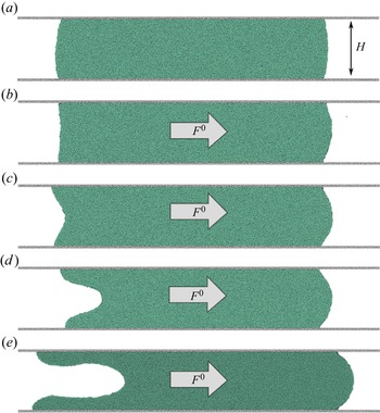

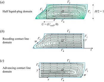


 Open access