


1. Introduction
Flow interactions are thought to play an important role in the locomotion of highly ordered animal groups, such as schools of fish and flight formations of birds. A popular belief is that the group is able to reduce on the energetic cost needed to move through the fluid by taking advantage of the collectively generated flows. For example, individual birds in a V-formation are thought to exploit the upward flow or upwash generated by neighbouring birds to generate the required lift with reduced effort (Lissaman & Shollenberger Reference Lissaman and Shollenberger1970; Weimerskirch et al. Reference Weimerskirch, Martin, Clerquin, Alexandre and Jiraskova2001; Portugal et al. Reference Portugal, Hubel, Fritz, Heese, Trobe, Voelkl, Hailes, Wilson and Usherwood2014). For fish schools, an increasing number of studies show that individuals in a group gain energetic benefits compared with swimming alone (Belyayev & Zuyev Reference Belyayev and Zuyev1969; Zuyev & Belyayev Reference Zuyev and Belyayev1970; Svendsen et al. Reference Svendsen, Skov, Bildsoe and Steffensen2003; Killen et al. Reference Killen, Marras, Steffensen and McKenzie2012). An early theory argues that each fish extracts energy from the vortical flows created by others, and predicts a particularly favourable arrangement is a diamond-shaped lattice (Weihs Reference Weihs1973, Reference Weihs1975). Although this optimal configuration has not been observed in field and laboratory studies (Partridge & Pitcher Reference Partridge and Pitcher1979), efficiency improvement due to vortex–swimmer interactions has been seen in modelling and simulation studies (Hemelrijk et al. Reference Hemelrijk, Reid, Hildenbrandt and Padding2015; Daghooghi & Borazjani Reference Daghooghi and Borazjani2015).
Studies have made progress by considering the simplified problem of a single body swimming or flying within ambient vortices. Experiments have shown that trout swimming in a von Kármán wake behind a bluff body tend to slalom between vortex cores, and measurements showing reduced muscle activity suggest that flow effects are being exploited (Liao et al. Reference Liao, Beal, Lauder and Triantafyllou2003; Liao Reference Liao2007). Theoretical modelling has examined a flexible filament swimming in a vortex street, where the thrust or efficiency can be maximised with respect to the flapping kinematics (Alben Reference Alben2009a
, Reference Alben2010a
). Other studies focus on a pair of flapping and interacting bodies, for example, a pair of passively flapping filaments (Ristroph & Zhang Reference Ristroph and Zhang2008; Alben Reference Alben2009c
, Reference Alben2012), as well as actively flapping wings or foils placed side-by-side (Dewey et al. Reference Dewey, Quinn, Boschitsch and Smits2014) or in tandem (Akhtar et al. Reference Akhtar, Mittal, Lauder and Drucker2007; Boschitsch, Dewey & Smits Reference Boschitsch, Dewey and Smits2014). Interactions of freely swimming and actively flapping bodies were studied in computational fluid dynamics simulations (Zhu, He & Zhang Reference Zhu, He and Zhang2014). A pair of actively flapping and flexible filaments swimming freely in tandem revealed the formation of stable configurations of reduced energetic input. Although Zhu et al. (Reference Zhu, He and Zhang2014) used a somewhat low Reynolds number ( $Re=200$
), similar stable configurations of tandem flapping hydrofoils were observed in experiments at the higher Reynolds numbers (
$Re=200$
), similar stable configurations of tandem flapping hydrofoils were observed in experiments at the higher Reynolds numbers ( $Re=10^4 \sim 10^5$
) typical of schools and flocks (Becker et al. Reference Becker, Masoud, Newbolt, Shelley and Ristroph2015; Ramananarivo et al. Reference Ramananarivo, Fang, Oza, Zhang and Ristroph2016).
$Re=10^4 \sim 10^5$
) typical of schools and flocks (Becker et al. Reference Becker, Masoud, Newbolt, Shelley and Ristroph2015; Ramananarivo et al. Reference Ramananarivo, Fang, Oza, Zhang and Ristroph2016).
By using freely swimming and flapping hydrofoils in controlled experiments, Becker et al. (Reference Becker, Masoud, Newbolt, Shelley and Ristroph2015), Ramananarivo et al. (Reference Ramananarivo, Fang, Oza, Zhang and Ristroph2016), Newbolt, Zhang & Ristroph (Reference Newbolt, Zhang and Ristroph2019) and Newbolt et al. (Reference Newbolt, Lewis, Bleu, Wu, Mavroyiakoumou, Ramananarivo and Ristroph2024) sought to understand the flow interactions relevant to high- $Re$
collective locomotion. These studies build on previous ones that have characterised the locomotion of a single heaving foil (Vandenberghe, Zhang & Childress Reference Vandenberghe, Zhang and Childress2004; Alben & Shelley Reference Alben and Shelley2005; Vandenberghe, Childress & Zhang Reference Vandenberghe, Childress and Zhang2006). Such a locomotor leaves a stereotypical thrust wake consisting of an array of staggered and counter-rotating vortices, similar to that seen behind swimming fish (Müller et al. Reference Müller, Van Den Heuvel, Stamhuis and Videler1997). Becker et al. (Reference Becker, Masoud, Newbolt, Shelley and Ristroph2015) studied the hydrodynamic interactions and swimming dynamics of an in-line array of flapping foils held at fixed separation distances. Constructive and destructive wing–wake interactions were found to coexist and correspond to fast and slow swimming modes of the group, respectively. Introducing the so-called schooling number
$Re$
collective locomotion. These studies build on previous ones that have characterised the locomotion of a single heaving foil (Vandenberghe, Zhang & Childress Reference Vandenberghe, Zhang and Childress2004; Alben & Shelley Reference Alben and Shelley2005; Vandenberghe, Childress & Zhang Reference Vandenberghe, Childress and Zhang2006). Such a locomotor leaves a stereotypical thrust wake consisting of an array of staggered and counter-rotating vortices, similar to that seen behind swimming fish (Müller et al. Reference Müller, Van Den Heuvel, Stamhuis and Videler1997). Becker et al. (Reference Becker, Masoud, Newbolt, Shelley and Ristroph2015) studied the hydrodynamic interactions and swimming dynamics of an in-line array of flapping foils held at fixed separation distances. Constructive and destructive wing–wake interactions were found to coexist and correspond to fast and slow swimming modes of the group, respectively. Introducing the so-called schooling number $S$
, defined as the inter-neighbour separation distance normalised by the wavelength of the swimming trajectory, it was observed that the array assumed
$S$
, defined as the inter-neighbour separation distance normalised by the wavelength of the swimming trajectory, it was observed that the array assumed $S$
values only between integer to half-integer values, which may be associated with stable wing–wake interactions. This was investigated theoretically by Oza, Ristroph & Shelley (Reference Oza, Ristroph and Shelley2019) using a discrete-time dynamical system, which showed good agreement with the experimental data, in particular predicting the bistability of schooling states. The importance of hydrodynamic stability in collective locomotion, heretofore rarely discussed in the literature, was further investigated by Ramananarivo et al. (Reference Ramananarivo, Fang, Oza, Zhang and Ristroph2016) for the case of tandem flapping foils. In this experimental realisation of the simplest ‘school of two’, the wings are freely swimming and freely spacing. The emergent stable configurations involve the pair travelling together with constant separation and with integer schooling numbers, i.e. the wings maintain a separation distance that is an integer multiple of the motion wavelength. Ramananarivo et al. (Reference Ramananarivo, Fang, Oza, Zhang and Ristroph2016) also measured directly the hydrodynamic restoring forces on the follower and for the first time determined the hydrodynamic potential felt by a locomotor interacting with the wake of a leader. Newbolt et al. (Reference Newbolt, Zhang and Ristroph2019) investigated the flow interactions between uncoordinated flapping foils with different kinematics, showing that these interactions can spontaneously lead to group cohesion. When the leader and follower flap asynchronously – with a non-zero phase lag
$S$
values only between integer to half-integer values, which may be associated with stable wing–wake interactions. This was investigated theoretically by Oza, Ristroph & Shelley (Reference Oza, Ristroph and Shelley2019) using a discrete-time dynamical system, which showed good agreement with the experimental data, in particular predicting the bistability of schooling states. The importance of hydrodynamic stability in collective locomotion, heretofore rarely discussed in the literature, was further investigated by Ramananarivo et al. (Reference Ramananarivo, Fang, Oza, Zhang and Ristroph2016) for the case of tandem flapping foils. In this experimental realisation of the simplest ‘school of two’, the wings are freely swimming and freely spacing. The emergent stable configurations involve the pair travelling together with constant separation and with integer schooling numbers, i.e. the wings maintain a separation distance that is an integer multiple of the motion wavelength. Ramananarivo et al. (Reference Ramananarivo, Fang, Oza, Zhang and Ristroph2016) also measured directly the hydrodynamic restoring forces on the follower and for the first time determined the hydrodynamic potential felt by a locomotor interacting with the wake of a leader. Newbolt et al. (Reference Newbolt, Zhang and Ristroph2019) investigated the flow interactions between uncoordinated flapping foils with different kinematics, showing that these interactions can spontaneously lead to group cohesion. When the leader and follower flap asynchronously – with a non-zero phase lag $\phi$
between their heaving motions – the follower settles into one of several discrete positions behind the leader, with the pair subsequently travelling together (Newbolt et al. Reference Newbolt, Zhang and Ristroph2019; Mavroyiakoumou, Wu & Ristroph Reference Mavroyiakoumou, Wu and Ristroph2025). As
$\phi$
between their heaving motions – the follower settles into one of several discrete positions behind the leader, with the pair subsequently travelling together (Newbolt et al. Reference Newbolt, Zhang and Ristroph2019; Mavroyiakoumou, Wu & Ristroph Reference Mavroyiakoumou, Wu and Ristroph2025). As $\phi$
increases, these stable positions are displaced downstream at a constant rate. A recent experimental study involving larger collectives (of up to five foils) demonstrated that chains of increasing size become unstable due to flow-induced instabilities termed flonons (Newbolt et al. Reference Newbolt, Lewis, Bleu, Wu, Mavroyiakoumou, Ramananarivo and Ristroph2024). In this phenomenon, the horizontal positions of downstream foils begin to oscillate with progressively larger amplitudes down the group, potentially leading to collisions between the trailing members. This instability was subsequently found numerically using a vortex-sheet model in Nitsche, Oza & Siegel (Reference Nitsche, Oza and Siegel2025).
$\phi$
increases, these stable positions are displaced downstream at a constant rate. A recent experimental study involving larger collectives (of up to five foils) demonstrated that chains of increasing size become unstable due to flow-induced instabilities termed flonons (Newbolt et al. Reference Newbolt, Lewis, Bleu, Wu, Mavroyiakoumou, Ramananarivo and Ristroph2024). In this phenomenon, the horizontal positions of downstream foils begin to oscillate with progressively larger amplitudes down the group, potentially leading to collisions between the trailing members. This instability was subsequently found numerically using a vortex-sheet model in Nitsche, Oza & Siegel (Reference Nitsche, Oza and Siegel2025).
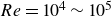
Interaction of a pair of flapping wings in tandem. Two wings, modelled as slender rigid plates, heave with prescribed vertical motions and are individually free to translate in the horizontal direction. Without loss of generality, we assume the wings swim or fly from right to left. Here, $A_k$
is the prescribed heaving amplitude,
$A_k$
is the prescribed heaving amplitude, $U_k$
is the emergent swimming speed (with
$U_k$
is the emergent swimming speed (with $k=1,2$
),
$k=1,2$
), $c$
is the chord length of each of the rigid plates,
$c$
is the chord length of each of the rigid plates, $g$
is the ‘tail-head’ separation distance and
$g$
is the ‘tail-head’ separation distance and $d$
is the separation distance between the wing centre points (or any equivalent points on the two wings).
$d$
is the separation distance between the wing centre points (or any equivalent points on the two wings).

Inspired by these previous studies, we investigate theoretically the interactions and collective dynamics of a tandem pair of free flapping wings swimming or flying through a fluid. In simulations and a model, we consider two identical and infinitesimally thin plates that are driven up and down vertically (i.e. heaving) in a two-dimensional inviscid and incompressible flow (see figure 1). A follower wing is placed directly downstream of a leader, and the two have identical flapping frequency and temporal phase but perhaps different amplitudes. The wings are individually self-propelled and swim or fly in the horizontal direction, and the two are coupled only through their collective flow field. Our numerical results complement prior work on vortex-sheet simulations of inline flapping plates by Heydari & Kanso (Reference Heydari and Kanso2021) and Nitsche et al. (Reference Nitsche, Oza and Siegel2025), in several ways. Here, we investigate the steady-state velocities and positions of the plates as functions of drag coefficient and heaving amplitude across a wide range of drag coefficients, and we characterise the steady states as potential wells within a potential landscape.
In the first half of this paper, we discuss numerical simulations that use a two-dimensional (2-D) vortex-sheet method to study fluid–structure interactions at high $Re$
. We follow the scheme described in Fang et al. (Reference Fang, Ho, Ristroph and Shelley2017) that incorporates the fast multipole method (FMM) to efficiently simulate the complex vortical flow fields generated by a dynamic body, and its interaction with these flows. The quadrature rules are improved by applying singularity subtractions and piece-wise analytic evaluations to prevent vortex-sheet penetration at the wing boundaries. The Blasius skin-friction calculation (Schlichting Reference Schlichting1968) is coupled with this scheme as a model of viscous drag on each wing, permitting the study of steady states set by force balance. Our simulations confirm previous numerical and experimental results (Zhu et al. Reference Zhu, He and Zhang2014; Ramananarivo et al. Reference Ramananarivo, Fang, Oza, Zhang and Ristroph2016; Newbolt et al. Reference Newbolt, Zhang and Ristroph2019; Heydari & Kanso Reference Heydari and Kanso2021) of multiple stable configurations, called ‘schooling states’ in what follows. We also map out an effective hydrodynamic potential on the follower wing using two strategies, and find the hydrodynamic force on the follower is approximately a sinusoidal function of the schooling number
$Re$
. We follow the scheme described in Fang et al. (Reference Fang, Ho, Ristroph and Shelley2017) that incorporates the fast multipole method (FMM) to efficiently simulate the complex vortical flow fields generated by a dynamic body, and its interaction with these flows. The quadrature rules are improved by applying singularity subtractions and piece-wise analytic evaluations to prevent vortex-sheet penetration at the wing boundaries. The Blasius skin-friction calculation (Schlichting Reference Schlichting1968) is coupled with this scheme as a model of viscous drag on each wing, permitting the study of steady states set by force balance. Our simulations confirm previous numerical and experimental results (Zhu et al. Reference Zhu, He and Zhang2014; Ramananarivo et al. Reference Ramananarivo, Fang, Oza, Zhang and Ristroph2016; Newbolt et al. Reference Newbolt, Zhang and Ristroph2019; Heydari & Kanso Reference Heydari and Kanso2021) of multiple stable configurations, called ‘schooling states’ in what follows. We also map out an effective hydrodynamic potential on the follower wing using two strategies, and find the hydrodynamic force on the follower is approximately a sinusoidal function of the schooling number $S$
, defined as the tail-to-head wing separation normalised by the locomotion wavelength. The hydrodynamic potential consists of multiple wells corresponding to the multiple stable states. Investigation of the emergent flow fields shows that, when the follower’s flapping motion is in phase with the oscillatory flow left by the leader, the collective wake is constructively reinforced but the follower produces low thrust. In contrast, for out-of-phase motions with the oncoming flow, the follower produces larger thrust as the collective wake is weakened. We show how these effects can be exploited by a follower with low flapping amplitude swimming behind a fast-flapping leader. Surprisingly, this ‘freeloading’ follower is still able to keep up with the leader, as it passively relocates to a favourable position in the leader’s wake. A significant improvement in swimming efficiency is observed in this situation, with the follower even harvesting energy from the wake of the leader.
$S$
, defined as the tail-to-head wing separation normalised by the locomotion wavelength. The hydrodynamic potential consists of multiple wells corresponding to the multiple stable states. Investigation of the emergent flow fields shows that, when the follower’s flapping motion is in phase with the oscillatory flow left by the leader, the collective wake is constructively reinforced but the follower produces low thrust. In contrast, for out-of-phase motions with the oncoming flow, the follower produces larger thrust as the collective wake is weakened. We show how these effects can be exploited by a follower with low flapping amplitude swimming behind a fast-flapping leader. Surprisingly, this ‘freeloading’ follower is still able to keep up with the leader, as it passively relocates to a favourable position in the leader’s wake. A significant improvement in swimming efficiency is observed in this situation, with the follower even harvesting energy from the wake of the leader.
In the second half of this paper, we calculate analytically the stable states of the two-wing interaction and the hydrodynamic potential on the follower wing using a linearised theory that assumes small flapping amplitude and large wavelength of motion. The linearised Euler equation with a no-penetration boundary condition imposed on a plate was analytically solved by Wu (Reference Wu1961). We combine Wu’s solution with a skin-friction model to determine the free-swimming speed of an isolated flapping wing. Motivated by the simulation results, we use the calculations of the isolated wing and its generated wake as approximations to the leader wing and its wake. We then adapt a second calculation of Wu for the thrust on a flapping wing in a wavy stream (Wu Reference Wu1972; Wu & Chwang Reference Wu and Chwang1975) to the interaction of the follower wing with the wavy wake generated by the leader. We provide an analytic expression of the effective hydrodynamic potential on the follower wing, and stable states and the ‘keep-up’ condition for a low-amplitude follower are also determined. We also include a more comprehensive comparison between the numerical results and these small-amplitude linearised theories. We find excellent agreement in the steady-state velocities and Froude efficiency for a single self-propelled flapping wing, and in the steady-state schooling number for the two-wing case.
2. Simulation method
Efficient simulations of high Reynolds number flows are challenging due to the associated complex vortex dynamics (Saffman Reference Saffman1993). In our study, we use an inviscid 2-D vortex-sheet model to capture both the vorticity distribution along the wings (called the bound sheet, as defined later) and the free vortex wake (the free sheet), as well as the unsteady shedding of vorticity from the wing trailing edge. Within this 2-D model, a vortex sheet is a 1-D boundary across which the fluid normal velocity is continuous while the tangential velocity is not (Rosenhead Reference Rosenhead1931; Saffman Reference Saffman1993). A stabilised 2-D vortex-sheet model was first proposed by Krasny (Reference Krasny1986) using a kernel regularisation technique. Combined with the unsteady Kutta condition, this method is widely used for fluid–structure interaction problems at high Re, for example in simulations of a jet flow exiting a tube (Nitsche & Krasny Reference Nitsche and Krasny1994), free falling plates (Jones Reference Jones2003; Jones & Shelley Reference Jones and Shelley2005), passively flapping filaments (Alben & Shelley Reference Alben and Shelley2008; Alben Reference Alben2009b ) and free flying jellyfish-like machines (Fang et al. Reference Fang, Ho, Ristroph and Shelley2017). In this work, we build on the vortex-sheet formulation for wing-pair interactions and free locomotion described by Fang et al. (Reference Fang, Ho, Ristroph and Shelley2017), and we implement a robust numerical algorithm using the FMM. To account for viscous effects and drag, we also include a Blasius skin-friction model (Schlichting Reference Schlichting1968). For each individual wing, the balance of the skin-friction drag and computed thrust from the vortex sheet determines the dynamics of the wing in the horizontal direction. We also improve the quadrature rules in the vortex-sheet method, by applying singularity subtractions on the body and piece-wise analytic evaluations on the wake, so as to prevent vortex-sheet penetration at the wing boundaries.
2.1. Modelling
2.1.1. Wing model and fluid model
As shown in figure 1, the pair of wings in tandem are each modelled as rigid plates of the same chord length $c$
. The up-and-down or heaving motions are prescribed by sinusoidal functions of the same frequency
$c$
. The up-and-down or heaving motions are prescribed by sinusoidal functions of the same frequency $f$
and (perhaps different) amplitudes
$f$
and (perhaps different) amplitudes $A_k$
$A_k$
 \begin{align} x_{k}(s,t) & = X_k(t)+s, \; s\in [-c/2,c/2], \end{align}
 \begin{align} y_{k}(t) & = A_k\cos (2\pi ft), \end{align}
where $k=1,2$
denotes the leader and follower wings, respectively, and
$k=1,2$
denotes the leader and follower wings, respectively, and $\boldsymbol{x}_k=(x_k,y_k)$
denotes their locations. Here,
$\boldsymbol{x}_k=(x_k,y_k)$
denotes their locations. Here, $y_k(t)$
is the same throughout the wing’s chord length (i.e. for any
$y_k(t)$
is the same throughout the wing’s chord length (i.e. for any $s\in [-c/2,c/2]$
of each wing), and so it is a function of time only. The arc-length parameter
$s\in [-c/2,c/2]$
of each wing), and so it is a function of time only. The arc-length parameter $s$
denotes the signed distance from the wing centre
$s$
denotes the signed distance from the wing centre $X_k(t)= x_k(0,t)$
. The leading edge of the wings (left end of the wing in figure 1) corresponds to
$X_k(t)= x_k(0,t)$
. The leading edge of the wings (left end of the wing in figure 1) corresponds to $s=-c/2$
, and the trailing edge (right end) corresponds to
$s=-c/2$
, and the trailing edge (right end) corresponds to $s=c/2$
.
$s=c/2$
.
The wings are individually free to swim or fly, that is, to move in the horizontal direction due to hydrodynamic interactions. Assuming a wing mass per unit span of $m$
, the horizontal dynamics of each individual satisfies
$m$
, the horizontal dynamics of each individual satisfies
 \begin{align} m\ddot {X}_k = F_k = T_k+D_k,\quad k=1,2, \end{align}
where $F_k$
is the hydrodynamic force on the wing, composed of the hydrodynamic thrust
$F_k$
is the hydrodynamic force on the wing, composed of the hydrodynamic thrust $T_k$
and drag
$T_k$
and drag $D_k$
. Here, the propulsive thrust is negatively signed and the resistive drag is positively signed, given the convention that the wings swim or fly from right to left.
$D_k$
. Here, the propulsive thrust is negatively signed and the resistive drag is positively signed, given the convention that the wings swim or fly from right to left.
The surrounding inviscid fluid flow is described by the 2-D Euler equations
 \begin{align} \rho _{f}\frac {{\rm D}\boldsymbol{u}}{{\rm D}t}=-\boldsymbol{\nabla }p, \end{align}
where $\boldsymbol{u}=(u_x,u_y)$
is the fluid velocity,
$\boldsymbol{u}=(u_x,u_y)$
is the fluid velocity, $p$
is the pressure and
$p$
is the pressure and $\rho _{f}$
is the fluid density. We impose a no-penetration boundary condition for the flow velocity
$\rho _{f}$
is the fluid density. We impose a no-penetration boundary condition for the flow velocity $\boldsymbol{u}(\boldsymbol{x}(s))$
on each wing, with the vertical component of the velocity being continuous and matching the wing flapping speed, in a reference frame where the fluid is at rest at infinity. That is, the vertical components
$\boldsymbol{u}(\boldsymbol{x}(s))$
on each wing, with the vertical component of the velocity being continuous and matching the wing flapping speed, in a reference frame where the fluid is at rest at infinity. That is, the vertical components $u_{y,\pm }$
above and below the wing are equal to the vertical component of the wing velocity
$u_{y,\pm }$
above and below the wing are equal to the vertical component of the wing velocity
 \begin{eqnarray} u_{y,+}(\boldsymbol{x}_k(s,t))=u_{y,-}(\boldsymbol{x}_k(s,t))=\dot {y}_k(t),\quad k=1,2. \end{eqnarray}
In the tangential direction at the wing, i.e. the $x$
-direction, flow is allowed to slip freely along the surface. This horizontal component
$x$
-direction, flow is allowed to slip freely along the surface. This horizontal component $u_{x,\pm }(\boldsymbol{x}_k(s,t))$
of the flow velocity can be viewed as a model for the flow just outside of the boundary layer, which approaches zero thickness in the limit of infinite Reynolds number. We later discuss a skin-friction model that estimates the drag due to shear in the viscous boundary layer.
$u_{x,\pm }(\boldsymbol{x}_k(s,t))$
of the flow velocity can be viewed as a model for the flow just outside of the boundary layer, which approaches zero thickness in the limit of infinite Reynolds number. We later discuss a skin-friction model that estimates the drag due to shear in the viscous boundary layer.
Integration of the fluid pressure over a closed contour around each wing surface $C_k^w$
provides the thrust, i.e. the hydrodynamic force in the horizontal or tangential direction
$C_k^w$
provides the thrust, i.e. the hydrodynamic force in the horizontal or tangential direction $\hat {\boldsymbol{s}}=(1,0)$
. This integral can be separated into parts associated with an infinitesimal circle (denoted by
$\hat {\boldsymbol{s}}=(1,0)$
. This integral can be separated into parts associated with an infinitesimal circle (denoted by $r_k^{le}$
) around the wing’s leading edge, the differential or jump in pressure
$r_k^{le}$
) around the wing’s leading edge, the differential or jump in pressure $[p]$
across the length of the wing and an infinitesimal circle
$[p]$
across the length of the wing and an infinitesimal circle $r_k^{te}$
at the trailing edge
$r_k^{te}$
at the trailing edge
 \begin{align} \int _{C_k^w}p\hat {\boldsymbol{n}}\,{\mathrm{d}} s \boldsymbol{\cdot }\hat {\boldsymbol{s}}=\left ( \int _{r_k^{le}}p\hat {\boldsymbol{n}}\,{\mathrm{d}} s +\int _{-1}^1[p]\hat {\boldsymbol{n}}\,{\mathrm{d}} s + \int _{r_k^{te}}p\hat {\boldsymbol{n}}\,{\mathrm{d}} s \right ) \boldsymbol{\cdot }\hat {\boldsymbol{s}}, \quad \hat {\boldsymbol{s}}=(1,0). \end{align}
In our model, we allow continuous shedding of vorticity at the trailing edge while keeping a flow singularity at the leading edge. The absence of leading-edge shedding is intended as a model applicable to the case of small-amplitude flapping and long wavelengths of motion, in which case the small angles of attack are associated with weak leading-edge separation. The singularity at the leading edge yields a leading-edge suction and thrust in the tangential direction to the wing (Saffman Reference Saffman1993). Note that the integral of the pressure jump $[p]$
along the wing is always normal to the wing and does not contribute to the thrust. The pressure integral around the wing trailing edge is also zero due to the imposition of the unsteady Kutta condition. Therefore, for a heaving wing that swims in a direction parallel to the body axis, the thrust results purely from leading-edge suction. Thus, (2.6) simplifies to
$[p]$
along the wing is always normal to the wing and does not contribute to the thrust. The pressure integral around the wing trailing edge is also zero due to the imposition of the unsteady Kutta condition. Therefore, for a heaving wing that swims in a direction parallel to the body axis, the thrust results purely from leading-edge suction. Thus, (2.6) simplifies to
 \begin{align} T_k =\int _{C_k^w}p\hat {\boldsymbol{n}}\,{\mathrm{d}} s \boldsymbol{\cdot }\hat {\boldsymbol{s}} =\int _{r_k^{le}}p\hat {\boldsymbol{n}}\,{\mathrm{d}} s \boldsymbol{\cdot }\hat {\boldsymbol{s}}, \quad \hat {\boldsymbol{s}}=(1,0). \end{align}
The hydrodynamic drag in (2.3) results from skin friction along the upper and lower wing surfaces, which is modelled using Blasius laminar boundary-layer theory (Schlichting Reference Schlichting1968, Chap. VII). For one side of a plate in a stream of uniform far-field speed $U_f$
, this approximation gives
$U_f$
, this approximation gives
 \begin{align} D_f=0.664\sqrt {\rho _{f}\mu c}\,| U_f|^{3/2}, \end{align}
where $\mu$
is the dynamic viscosity of the fluid. In our model, we replace the free-stream velocity
$\mu$
is the dynamic viscosity of the fluid. In our model, we replace the free-stream velocity $U_f$
with the tangential flow speed averaged along the wing surface and relative to the swimming speed
$U_f$
with the tangential flow speed averaged along the wing surface and relative to the swimming speed
 \begin{align} \overline {U}_{k,\pm }(t) = \frac {1}{c}\int _{-c/2}^{c/2}u_{x,\pm }(\boldsymbol{x}_k(s,t))\,{\mathrm{d}} s-U_k(t), \end{align}
where $U_k(t)=\dot {X}_{k}(t)$
is the horizontal swimming speed of the wing, which is assumed to move in the negative
$U_k(t)=\dot {X}_{k}(t)$
is the horizontal swimming speed of the wing, which is assumed to move in the negative $x$
-direction (figure 1). Summing the contributions from the upper and lower surfaces of the wing, the total drag is
$x$
-direction (figure 1). Summing the contributions from the upper and lower surfaces of the wing, the total drag is
 \begin{align} D_k=0.664\sqrt {\rho _{f}\mu c}\,\left (|\overline {U}_{k,+}|^{3/2}+|\overline {U}_{k,-}|^{3/2}\right ). \end{align}
This form of the drag force was also implemented by Heydari & Kanso (Reference Heydari and Kanso2021). We note that the drag force scaling with $U^{3/2}$
reproduces the experimentally observed
$U^{3/2}$
reproduces the experimentally observed $(Af)^{4/3}$
dependence of the swimming speed for a single heaving wing (Ramananarivo et al. Reference Ramananarivo, Fang, Oza, Zhang and Ristroph2016). This is consistent with the scaling identified by Gazzola, Argentina & Mahadevan (Reference Gazzola, Argentina and Mahadevan2014) for locomotion in the laminar-flow regime at Reynolds numbers up to approximately
$(Af)^{4/3}$
dependence of the swimming speed for a single heaving wing (Ramananarivo et al. Reference Ramananarivo, Fang, Oza, Zhang and Ristroph2016). This is consistent with the scaling identified by Gazzola, Argentina & Mahadevan (Reference Gazzola, Argentina and Mahadevan2014) for locomotion in the laminar-flow regime at Reynolds numbers up to approximately $10^4$
and where drag dominantly arises from skin friction due to laminar boundary-layer flows. At yet higher Reynolds numbers of the turbulent-flow regime, a quadratic drag law of the form
$10^4$
and where drag dominantly arises from skin friction due to laminar boundary-layer flows. At yet higher Reynolds numbers of the turbulent-flow regime, a quadratic drag law of the form $U^2$
is likely more appropriate and derives from pressure and separated flows (Gazzola et al. Reference Gazzola, Argentina and Mahadevan2014).
$U^2$
is likely more appropriate and derives from pressure and separated flows (Gazzola et al. Reference Gazzola, Argentina and Mahadevan2014).
We non-dimensionalise the system with the characteristic length $\tilde {L}=c/2,$
time
$\tilde {L}=c/2,$
time $\tilde {T}=1/f$
, velocity
$\tilde {T}=1/f$
, velocity $\tilde {U}=cf/2$
and pressure
$\tilde {U}=cf/2$
and pressure $P=\rho _f\tilde {U}^2=\rho _{f}c^{2}f^{2}/4.$
The dimensionless equations of motion are then
$P=\rho _f\tilde {U}^2=\rho _{f}c^{2}f^{2}/4.$
The dimensionless equations of motion are then
 \begin{align} M\ddot {X}_k & = T_k(t)+D_k(t), \end{align}
 \begin{eqnarray} y_{k}(s,t) & = \tilde {A}_k\cos (2\pi t),\ s\in [-1,1], \end{eqnarray}
where
 \begin{align} T_k = \int _{C_k^w}p\hat {\boldsymbol{n}}\,{\mathrm{d}} s\boldsymbol{\cdot }\hat {\boldsymbol{s}}\quad \text{and}\quad D_k = C_f\left (\overline {U}_{k,+}^{3/2}+\overline {U}_{k,-}^{3/2}\right ),\; \quad k=1,2. \end{align}
There are three dimensionless parameters that appear in the system: the wing–fluid mass ratio $M=4m/(\rho _fc^2)$
, the ratio of the heaving amplitude to wing length
$M=4m/(\rho _fc^2)$
, the ratio of the heaving amplitude to wing length $\tilde {A}_k = 2A_k/c$
and the skin-friction drag coefficient
$\tilde {A}_k = 2A_k/c$
and the skin-friction drag coefficient
 \begin{align} C_f = 1.878\sqrt {\nu /(c^2f)}, \end{align}
where $\nu =\mu /\rho _f$
is the kinematic viscosity. This drag coefficient is related to the so-called frequency Reynolds number
$\nu =\mu /\rho _f$
is the kinematic viscosity. This drag coefficient is related to the so-called frequency Reynolds number $Re_{fr}=\tilde {L}\tilde {U}/\nu =c^2f/4\nu$
used in the literature of flapping-wing locomotion (Alben & Shelley Reference Alben and Shelley2005):
$Re_{fr}=\tilde {L}\tilde {U}/\nu =c^2f/4\nu$
used in the literature of flapping-wing locomotion (Alben & Shelley Reference Alben and Shelley2005): $C_f=0.939Re_{fr}^{-1/2}$
. When the kinematics, wing chord length and fluid parameters are appropriately matched to the experimental conditions of Ramananarivo et al. (Reference Ramananarivo, Fang, Oza, Zhang and Ristroph2016), (2.14) yields
$C_f=0.939Re_{fr}^{-1/2}$
. When the kinematics, wing chord length and fluid parameters are appropriately matched to the experimental conditions of Ramananarivo et al. (Reference Ramananarivo, Fang, Oza, Zhang and Ristroph2016), (2.14) yields $C_{f}\sim 0.02$
, reproducing the same trends in swimming speed observed in the experiments. In our study, we set the mass ratio to
$C_{f}\sim 0.02$
, reproducing the same trends in swimming speed observed in the experiments. In our study, we set the mass ratio to $M=2$
while exploring the effects of varying
$M=2$
while exploring the effects of varying $C_{f}=0.01$
to
$C_{f}=0.01$
to $0.1$
and
$0.1$
and $\tilde {A}_{k}=0.1$
to
$\tilde {A}_{k}=0.1$
to $1$
. Here, the mass per unit span
$1$
. Here, the mass per unit span $m$
should be interpreted as the total solid mass of the locomotor (i.e. the free-swimming or flying animal), which sets the relevant inertia for the forward dynamics. We note that, even for an arbitrarily thin wing, a finite value of wing–fluid mass ratio
$m$
should be interpreted as the total solid mass of the locomotor (i.e. the free-swimming or flying animal), which sets the relevant inertia for the forward dynamics. We note that, even for an arbitrarily thin wing, a finite value of wing–fluid mass ratio $M$
remains meaningful because it represents the mass payload (e.g. the body of a fish or bird) that is towed by the propulsor (fin or wing). The choice of
$M$
remains meaningful because it represents the mass payload (e.g. the body of a fish or bird) that is towed by the propulsor (fin or wing). The choice of $M=2$
is not meant to match a specific biological system; rather, it lies within the range typical of swimming and flying animals (Greenewalt Reference Greenewalt1962; Rayner Reference Rayner1979; Viscor & Fuster Reference Viscor and Fuster1987; Dimitriadis et al. Reference Dimitriadis, Gardiner, Tickle, Codd and Nudds2015; Taylor et al. Reference Taylor, Taylor, Lambert, Walker, Biro and Portugal2019; Krishnan et al. Reference Krishnan2022) and is consistent with flapping-foil experiments and prior numerical studies (Ramananarivo et al. Reference Ramananarivo, Fang, Oza, Zhang and Ristroph2016; Newbolt et al. Reference Newbolt, Zhang and Ristroph2019, Reference Newbolt, Lewis, Bleu, Wu, Mavroyiakoumou, Ramananarivo and Ristroph2024; Nitsche et al. Reference Nitsche, Oza and Siegel2025). A smaller mass, and thus lower inertia, is expected to make the wing more susceptible to fluctuations. This leads to larger oscillations in the separation gap between the wings, which could undermine the positional stabilisation of the wing. The influence of mass will be examined further in future work.
$M=2$
is not meant to match a specific biological system; rather, it lies within the range typical of swimming and flying animals (Greenewalt Reference Greenewalt1962; Rayner Reference Rayner1979; Viscor & Fuster Reference Viscor and Fuster1987; Dimitriadis et al. Reference Dimitriadis, Gardiner, Tickle, Codd and Nudds2015; Taylor et al. Reference Taylor, Taylor, Lambert, Walker, Biro and Portugal2019; Krishnan et al. Reference Krishnan2022) and is consistent with flapping-foil experiments and prior numerical studies (Ramananarivo et al. Reference Ramananarivo, Fang, Oza, Zhang and Ristroph2016; Newbolt et al. Reference Newbolt, Zhang and Ristroph2019, Reference Newbolt, Lewis, Bleu, Wu, Mavroyiakoumou, Ramananarivo and Ristroph2024; Nitsche et al. Reference Nitsche, Oza and Siegel2025). A smaller mass, and thus lower inertia, is expected to make the wing more susceptible to fluctuations. This leads to larger oscillations in the separation gap between the wings, which could undermine the positional stabilisation of the wing. The influence of mass will be examined further in future work.
2.1.2. Vortex-sheet shedding and wake model
In the vortex-sheet model, a flapping wing is a bound vortex sheet on which the no-penetration boundary condition (2.5) is imposed. The bound sheet encompasses the infinitesimally thin wing and its boundary layers that vanish in thickness at higher Reynolds numbers. At the trailing edge of each wing, a free vortex sheet is continuously shed into the fluid (Nitsche & Krasny Reference Nitsche and Krasny1994). In the free-sheet model the shed shear layer forms downstream eddies. In the limit of zero viscosity, the shed vorticity concentrates onto an infinitesimally thin layer that can be modelled as a 1-D vortex sheet that does not dissipate in time. The vortex shedding rate at the trailing edge is determined by the unsteady Kutta condition (Jones Reference Jones2003), which provides the direction of vortex shedding as well as the amount of circulation transmitted from the wing (bound sheet) to the wake (free sheet).
In our 2-D vortex-sheet method, we keep track of the sheet position $\zeta _k(s,t)$
as well as the true vortex-sheet strength
$\zeta _k(s,t)$
as well as the true vortex-sheet strength $\bar {\gamma }_k(s,t)$
, defined as the tangential fluid velocity jump across the vortex sheet
$\bar {\gamma }_k(s,t)$
, defined as the tangential fluid velocity jump across the vortex sheet $\bar {\gamma }_k(s,t)=[\boldsymbol{u}]\hat {s}$
(Shelley Reference Shelley1992). Here,
$\bar {\gamma }_k(s,t)=[\boldsymbol{u}]\hat {s}$
(Shelley Reference Shelley1992). Here, $k=1,2$
denotes the two wings, and
$k=1,2$
denotes the two wings, and $s\in [-1,s^k_{max }]$
is an arc-length parameterisation of the vortex sheet. The true vortex-sheet strength
$s\in [-1,s^k_{max }]$
is an arc-length parameterisation of the vortex sheet. The true vortex-sheet strength $\bar {\gamma }_k(s,t)=\gamma _k(\alpha )/s_{\alpha }(\alpha ,t)$
is related to the (unnormalised) vortex strength
$\bar {\gamma }_k(s,t)=\gamma _k(\alpha )/s_{\alpha }(\alpha ,t)$
is related to the (unnormalised) vortex strength $\gamma _k(\alpha )$
which is a material variable, where
$\gamma _k(\alpha )$
which is a material variable, where $\alpha$
is a Lagrangian parameterisation of the sheet. Using complex variables, the vortex-sheet position
$\alpha$
is a Lagrangian parameterisation of the sheet. Using complex variables, the vortex-sheet position $\zeta _k(s,t)$
and strength
$\zeta _k(s,t)$
and strength $\bar {\gamma }_k(s,t)$
are related through the Biot–Savart law for the mean velocity of the sheet
$\bar {\gamma }_k(s,t)$
are related through the Biot–Savart law for the mean velocity of the sheet $w_k(s,t)$
 \begin{align} \overline {w_k(s,t)} = \frac {1}{2\pi i}-\!\!\!\!\!\kern-1pt\int_{-1}^{{s}_{max}^{k}}\frac {\bar {\gamma }_{k}(s',t)\,{\mathrm{d}} s'}{\zeta _{k}(s,t)-\zeta _{k}(s',t)} +\sum _{j\neq k}\frac {1}{2\pi i}\int _{-1}^{s_{max }^j}\frac {\bar {\gamma }_{j}(s',t)\,{\mathrm{d}} s'}{\zeta _{k}(s,t)-\zeta _{j}(s',t)}, \end{align}
where the bar denotes the complex conjugate, and $ -\kern-1.5pt\!\!\!\!\int $
is the Cauchy principal value. Since the tangential component of fluid velocity is discontinuous at the vortex sheet, the mean velocity
$ -\kern-1.5pt\!\!\!\!\int $
is the Cauchy principal value. Since the tangential component of fluid velocity is discontinuous at the vortex sheet, the mean velocity $w_k(s,t)$
is an average of the velocities on the two sides of the sheet boundary
$w_k(s,t)$
is an average of the velocities on the two sides of the sheet boundary $\zeta _k(s,t)$
.
$\zeta _k(s,t)$
.
The description of the free-sheet boundary $s\in [1,s^k_{max }]$
dynamics is simplified if
$s\in [1,s^k_{max }]$
dynamics is simplified if $w_{k}(s,t)$
is chosen as a velocity frame, in which case we arrive at the Birkhoff–Rott equation (Shelley Reference Shelley1992)
$w_{k}(s,t)$
is chosen as a velocity frame, in which case we arrive at the Birkhoff–Rott equation (Shelley Reference Shelley1992)
 \begin{align} D_t\zeta _{k}(s,t) =w_{k}(s,t),\quad 1\leqslant s\leqslant s_{max }^k, \end{align}
where $D_t$
denotes the material derivative, and
$D_t$
denotes the material derivative, and $w_{k}(s,t)$
is given by (2.15). Following the Lagrangian path of the free vortex sheet, the circulation
$w_{k}(s,t)$
is given by (2.15). Following the Lagrangian path of the free vortex sheet, the circulation $\gamma (\alpha )$
on an infinitesimal segment is conserved
$\gamma (\alpha )$
on an infinitesimal segment is conserved
 \begin{align} D_t(\bar {\gamma }_{k}(s,t) s_{\alpha })=D_t\gamma _{k}(\alpha )=0,\quad k=1,2. \end{align}
The bound vortex-sheet position, i.e. the wing position
 \begin{align} \zeta _{k}(s,t) = X_k(t)+s+iy_k(t),\quad s\in [-1,1], \end{align}
is governed by (2.11). Using (2.15), the no-penetration boundary condition of (2.5) yields
 \begin{align} \textrm {Im}\left (w_{k}(s,t)\right )=\dot {y}_k(t),\quad s\in [-1,1], \end{align}
which is a Fredholm integral equation of the first kind for the bound-sheet strength $\bar {\gamma }_k(s,t),\ s\in [-1,1]$
.
$\bar {\gamma }_k(s,t),\ s\in [-1,1]$
.
The unsteady Kutta condition connects the bound and free sheets at the trailing edge (Jones Reference Jones2003). It requires the vortex shedding to be tangential, i.e. the interface of the bound and free vortex sheets is smooth, and also determines the amount of circulation shed from the bound sheet into the free sheet
 \begin{align} \dot {\varGamma }_k(t)+\left [\textrm {Re}(w_k(1,t))-U_k(t)\right ]\bar {\gamma }_k(1,t)=0, \end{align}
where $\varGamma _k(t) = \int _{-1}^1\bar {\gamma }_k(s,t)\,{\mathrm{d}} s$
denotes the total circulation on the bound sheet, and
$\varGamma _k(t) = \int _{-1}^1\bar {\gamma }_k(s,t)\,{\mathrm{d}} s$
denotes the total circulation on the bound sheet, and $U_k(t)=\dot {X}_{k}(t)$
is the wing horizontal swimming speed. Kelvin’s circulation conservation theorem ensures that
$U_k(t)=\dot {X}_{k}(t)$
is the wing horizontal swimming speed. Kelvin’s circulation conservation theorem ensures that $\varGamma _k(t) = -\int _1^{s_{max }^k}\bar {\gamma }_k(s,t)\,{\mathrm{d}} s$
.
$\varGamma _k(t) = -\int _1^{s_{max }^k}\bar {\gamma }_k(s,t)\,{\mathrm{d}} s$
.
An equation for the pressure jump $[p]_{k}(s,t)$
distributed on the bound sheet can be derived from the Euler equation (2.4) (Saffman Reference Saffman1993; Jones Reference Jones2003; Alben Reference Alben2009b
) and the Kutta condition (2.20)
$[p]_{k}(s,t)$
distributed on the bound sheet can be derived from the Euler equation (2.4) (Saffman Reference Saffman1993; Jones Reference Jones2003; Alben Reference Alben2009b
) and the Kutta condition (2.20)
 \begin{align} [p]_{k}(s,t)=\int _{1}^{s}\partial _{t}\bar {\gamma }_{k}(s',t)\,{\mathrm{d}} s'+\left [\textrm {Re}(w_k(s,t))-U_k(t)\right ]\bar {\gamma }_{k}(s,t)+\dot {\varGamma }_{k}(t). \end{align}
Note that the pressure jump across the wing contributes no force in the wing swimming direction, as the wing maintains a horizontal alignment at all times. The thrust arises from the suction force at the wing leading edge (Saffman Reference Saffman1993)
 \begin{align} T_k(t) = \frac {\pi }{8}\nu _k^{2}(-1,t), \end{align}
where $\nu _k(s,t)=\bar {\gamma }_k(s,t)\sqrt {1-s^2}$
has a finite value at
$\nu _k(s,t)=\bar {\gamma }_k(s,t)\sqrt {1-s^2}$
has a finite value at $s=-1$
as
$s=-1$
as $\bar {\gamma }_k$
has an inverse square root singularity at the wing leading edge. A full derivation of the leading-edge suction term can be found in Appendix A of Nitsche et al. (Reference Nitsche, Oza and Siegel2025). Note that (2.22) relates the hydrodynamics with the wing dynamics through (2.11).
$\bar {\gamma }_k$
has an inverse square root singularity at the wing leading edge. A full derivation of the leading-edge suction term can be found in Appendix A of Nitsche et al. (Reference Nitsche, Oza and Siegel2025). Note that (2.22) relates the hydrodynamics with the wing dynamics through (2.11).
On each wing, the instantaneous input power $P_{k,{in}}$
is defined as the product of flapping speed
$P_{k,{in}}$
is defined as the product of flapping speed $\dot {y}_k$
and the pressure jump
$\dot {y}_k$
and the pressure jump $\int _{-1}^{1}[p]_k\,{\mathrm{d}} s$
, which reflects the energy required to maintain the prescribed flapping motion. The instantaneous output power
$\int _{-1}^{1}[p]_k\,{\mathrm{d}} s$
, which reflects the energy required to maintain the prescribed flapping motion. The instantaneous output power $P_{k,{out}}$
equals the rate of work done by the hydrodynamic thrust
$P_{k,{out}}$
equals the rate of work done by the hydrodynamic thrust $T_k$
on the wing at swimming speed
$T_k$
on the wing at swimming speed $U_k$
. Hence,
$U_k$
. Hence,
 \begin{align} P_{k,{in}}(t)&=-\dot {y}_k(t)\int _{-1}^{1}[p]_k(s,t)\,{\mathrm{d}} s, \end{align}
 \begin{align} P_{k,{out}}(t)=T_k(t)U_k(t)=\frac {\pi }{8}\nu _k^{2}(-1,t)U_k(t). \end{align}
The ratio of $P_{k,{in}}$
and
$P_{k,{in}}$
and $P_{k,{out}}$
gives the Froude efficiency on each wing
$P_{k,{out}}$
gives the Froude efficiency on each wing $\eta _k,\ k=1,2$
and also the efficiency for the pair
$\eta _k,\ k=1,2$
and also the efficiency for the pair $\eta$
(Lighthill Reference Lighthill1960; Wu Reference Wu1961)
$\eta$
(Lighthill Reference Lighthill1960; Wu Reference Wu1961)
 \begin{align} \eta _k=\frac {\langle P_{k,{out}}\rangle }{\langle P_{k,{in}}\rangle },\quad \eta =\frac {\langle P_{1,{out}}\rangle +\langle P_{2,{out}}\rangle }{\langle P_{1,{in}}\rangle +\langle P_{2,{in}}\rangle }, \end{align}
where $\langle \boldsymbol{\cdot }\rangle =\int _t^{t+1}(\boldsymbol{\cdot }) \,{\mathrm{d}} t'$
denotes the time average over a flapping stroke.
$\langle \boldsymbol{\cdot }\rangle =\int _t^{t+1}(\boldsymbol{\cdot }) \,{\mathrm{d}} t'$
denotes the time average over a flapping stroke.
In the end, we express the mean tangential flow speed along the wing $\overline {U}_{k,\pm }(t)$
(2.9) using vortex-sheet variables in order to calculate the skin-friction drag
$\overline {U}_{k,\pm }(t)$
(2.9) using vortex-sheet variables in order to calculate the skin-friction drag $D_k$
of (2.13). By the definitions of the mean velocity
$D_k$
of (2.13). By the definitions of the mean velocity $w_k(s,t)$
and vortex-sheet strength
$w_k(s,t)$
and vortex-sheet strength $\bar {\gamma }_k(s,t)$
, the tangential speed along the two surfaces of each wing
$\bar {\gamma }_k(s,t)$
, the tangential speed along the two surfaces of each wing $u_{x,\pm }(\zeta _k(s,t))$
satisfies
$u_{x,\pm }(\zeta _k(s,t))$
satisfies
 \begin{align} u_{x,+}(\zeta _k(s,t))+u_{x,-}(\zeta _k(s,t)) = 2\textrm {Re}(w_k(s,t)),\nonumber \\ u_{x,+}(\zeta _k(s,t))-u_{x,-}(\zeta _k(s,t)) = \bar {\gamma }_k(s,t), \end{align}
from which we obtain
 \begin{align} u_{x,\pm }(\zeta _k(s,t)) = \textrm {Re}(w_k(s,t))\pm \frac {1}{2}\bar {\gamma }_k(s,t). \end{align}
Substituting (2.27) into (2.9), $\overline {U}_{k,\pm }(t)$
is then expressed as
$\overline {U}_{k,\pm }(t)$
is then expressed as
 \begin{align} \overline {U}_{k,\pm }(t)=\frac {1}{2}\int _{-1}^{1}\textrm {Re}(w_k(s,t))\,{\mathrm{d}} s-U_k(t)\pm \frac {1}{4}\int _{-1}^{1}\bar {\gamma }_k(s,t)\,{\mathrm{d}} s. \end{align}
2.2. Numerical schemes
Our numerical schemes follow closely those described by Fang et al. (Reference Fang, Ho, Ristroph and Shelley2017) and build on similar methods that have been used to study single slender bodies undergoing unsteady motions at high Reynolds numbers (Jones & Shelley Reference Jones and Shelley2005; Alben & Shelley Reference Alben and Shelley2008; Alben Reference Alben2009b ). For the two-body interaction problem studied here, the follower’s body interacts with the vortex sheet shed by the leader. To prevent the sheet from penetrating the wing due to numerical errors, an accurate quadrature rule is required. In our simulations, we improve the numerical vortex-sheet method developed by Alben (Reference Alben2009b , Reference Alben2010b ) and Fang et al. (Reference Fang, Ho, Ristroph and Shelley2017) by applying a singularity subtraction method for the singular integral kernel on the bound vortex sheet and a piece-wise quadrature on the free sheets (see Appendix A). Moreover, the vortex-sheet scheme is combined with the skin-friction computation in our simulations to permit the study of steady-state motions that arise from force balance. In what follows, we outline the main steps of the numerical schemes.
We assume the fluid is initially at rest. The wings are initialised with horizontal velocity $U_1(0)=U_2(0)=U_0$
and wing–wing separation
$U_1(0)=U_2(0)=U_0$
and wing–wing separation $x_2(0)-x_1(0)=d_0$
, where
$x_2(0)-x_1(0)=d_0$
, where $d_0=d(0)$
, and
$d_0=d(0)$
, and $d(t)$
is defined as the horizontal separation between equivalent points on the two wings (see figure 1). The vortex-sheet strength is initially zero, and the free sheets are confined to the wing trailing edges, i.e.
$d(t)$
is defined as the horizontal separation between equivalent points on the two wings (see figure 1). The vortex-sheet strength is initially zero, and the free sheets are confined to the wing trailing edges, i.e. $\bar {\gamma }_k(s,t)|_{t=0}=0,\ s\in [-1,1]$
and
$\bar {\gamma }_k(s,t)|_{t=0}=0,\ s\in [-1,1]$
and $s^k_{max }|_{t=0}=1$
. After initialisation, at each time step we update the vortex sheets in two steps: (a) update the existing free sheets
$s^k_{max }|_{t=0}=1$
. After initialisation, at each time step we update the vortex sheets in two steps: (a) update the existing free sheets $(\zeta _{f,k},\bar {\gamma }_{f,k})$
by an explicit scheme; (b) solve and update the bound sheets
$(\zeta _{f,k},\bar {\gamma }_{f,k})$
by an explicit scheme; (b) solve and update the bound sheets $(X_k,\bar {\gamma }_{b,k})$
and wing circulation
$(X_k,\bar {\gamma }_{b,k})$
and wing circulation $\varGamma _k$
through an implicit nonlinear Broyden solver (Broyden Reference Broyden1965), and shed a vortex-sheet segment at the trailing edge into the free vortex sheet. Here, the subscripts
$\varGamma _k$
through an implicit nonlinear Broyden solver (Broyden Reference Broyden1965), and shed a vortex-sheet segment at the trailing edge into the free vortex sheet. Here, the subscripts $f$
and
$f$
and $b$
denote the free and bound sheets, respectively.
$b$
denote the free and bound sheets, respectively.
The free vortex sheets are discretised by Lagrangian points $\zeta _{f,k}^{j,n},\ 0\leqslant j\leqslant n$
at time
$\zeta _{f,k}^{j,n},\ 0\leqslant j\leqslant n$
at time $t_n$
. At each time step
$t_n$
. At each time step $t_j$
, a new vortex-sheet segment
$t_j$
, a new vortex-sheet segment $[\zeta _{f,k}^{j-1,j}, \zeta _{f,k}^{j,j}]$
is produced at each wing trailing edge (no segment shed at
$[\zeta _{f,k}^{j-1,j}, \zeta _{f,k}^{j,j}]$
is produced at each wing trailing edge (no segment shed at $t_0$
). The dynamics of the free sheet follows (2.16) and is numerically updated by a second-order explicit Adams–Bashforth method, except for the last segment which is newly generated at the last time step and is updated using an explicit Euler scheme. Based on (2.17), the vortex circulation on each vortex-sheet segment is conserved. Following this, on segment
$t_0$
). The dynamics of the free sheet follows (2.16) and is numerically updated by a second-order explicit Adams–Bashforth method, except for the last segment which is newly generated at the last time step and is updated using an explicit Euler scheme. Based on (2.17), the vortex circulation on each vortex-sheet segment is conserved. Following this, on segment $[\zeta _{f,k}^{j-1,n}, \zeta _{f,k}^{j,n}]$
the true vortex-sheet strength (circulation density)
$[\zeta _{f,k}^{j-1,n}, \zeta _{f,k}^{j,n}]$
the true vortex-sheet strength (circulation density) $\bar {\gamma }_{f,k}^{j,n}, 1\leqslant j\leqslant n$
, is calculated by dividing the circulation of the segment by the segment length. For the newly generated segment at time
$\bar {\gamma }_{f,k}^{j,n}, 1\leqslant j\leqslant n$
, is calculated by dividing the circulation of the segment by the segment length. For the newly generated segment at time $t_{n+1}$
,
$t_{n+1}$
, $[\zeta _{f,k}^{n,n+1}, \zeta _{f,k}^{n+1,n+1}]$
, the last end point
$[\zeta _{f,k}^{n,n+1}, \zeta _{f,k}^{n+1,n+1}]$
, the last end point $\zeta _{f,k}^{n+1,n+1}$
is the same as the wing trailing edge at time
$\zeta _{f,k}^{n+1,n+1}$
is the same as the wing trailing edge at time $t_{n+1}$
, and the circulation of the last segment is equal to
$t_{n+1}$
, and the circulation of the last segment is equal to $-(\varGamma _k^{n+1}-\varGamma _k^{n})$
, where both the trailing edge
$-(\varGamma _k^{n+1}-\varGamma _k^{n})$
, where both the trailing edge $\zeta _{f,k}^{n+1,n+1}$
and wing circulation
$\zeta _{f,k}^{n+1,n+1}$
and wing circulation $\varGamma _k^{n+1}$
at time
$\varGamma _k^{n+1}$
at time $t_{n+1}$
are solved in the implicit step next.
$t_{n+1}$
are solved in the implicit step next.
The bound vortex sheet, i.e. the flapping wing, is discretised using $m+1$
Chebyshev–Gauss–Lobatto nodes
$m+1$
Chebyshev–Gauss–Lobatto nodes
 \begin{align} s_{j}=\cos (\phi _{j}),\;\phi _{j}=\frac {j\pi }{m},\quad j=0,\ldots ,m, \end{align}
and the smooth function $\nu _k(s,t)=\bar {\gamma }_k(s,t)\sqrt {1-s^{2}}$
is approximated by the
$\nu _k(s,t)=\bar {\gamma }_k(s,t)\sqrt {1-s^{2}}$
is approximated by the $m$
th-order polynomial interpolated at
$m$
th-order polynomial interpolated at $s_i$
. Once the free sheets are updated, in the implicit step the wing position and speed
$s_i$
. Once the free sheets are updated, in the implicit step the wing position and speed $(X_k^n,U_k^n)\approx (X_k(t_n),U_k(t_n))$
, bound-sheet strength
$(X_k^n,U_k^n)\approx (X_k(t_n),U_k(t_n))$
, bound-sheet strength $\nu _k^{i,n}\approx \nu _k(s_i,t_n)$
and wing circulation
$\nu _k^{i,n}\approx \nu _k(s_i,t_n)$
and wing circulation $\varGamma _k^{n}\approx \varGamma _k(t_n)$
are solved to match the updated free vortex sheets. The Cauchy singular integral (2.19) and Kutta condition (2.20) together provide
$\varGamma _k^{n}\approx \varGamma _k(t_n)$
are solved to match the updated free vortex sheets. The Cauchy singular integral (2.19) and Kutta condition (2.20) together provide $2(m+1)$
equations for the variables
$2(m+1)$
equations for the variables $\nu _k^{i,n},\ i=1,\ldots ,m$
and
$\nu _k^{i,n},\ i=1,\ldots ,m$
and $\varGamma _k^{n}\approx \varGamma _k(t_n)$
(see Golberg Reference Golberg2013; Alben Reference Alben2009b
; Fang et al. Reference Fang, Ho, Ristroph and Shelley2017). The wing dynamical variables (see (2.11)) are discretised by a second-order Crank–Nicolson scheme, which then provides
$\varGamma _k^{n}\approx \varGamma _k(t_n)$
(see Golberg Reference Golberg2013; Alben Reference Alben2009b
; Fang et al. Reference Fang, Ho, Ristroph and Shelley2017). The wing dynamical variables (see (2.11)) are discretised by a second-order Crank–Nicolson scheme, which then provides $4$
equations for
$4$
equations for $(X_k^n,U_k^n)$
 \begin{align} 0 = X_k^{n+1}-X_k^{n}-\frac {\triangle t}{2}(U_k^{n+1}+U_k^{n}),\quad 0 = U_k^{n+1}-U_k^{n}-\frac {\triangle t}{2M}(F_k^{n+1}+F_k^{n}),\quad k=1,2, \end{align}
where $F_k^{n}\approx F_k(t_{n})=T_k(t_{n})+D_k(t_{n})$
is the horizontal component of force on the wing, calculated using (2.13), (2.22) and (2.28). This completes a nonlinear system for
$F_k^{n}\approx F_k(t_{n})=T_k(t_{n})+D_k(t_{n})$
is the horizontal component of force on the wing, calculated using (2.13), (2.22) and (2.28). This completes a nonlinear system for $2(m+1)+4$
variables for the bound vortex sheets. Using Broyden’s method, the solution is found to converge to
$2(m+1)+4$
variables for the bound vortex sheets. Using Broyden’s method, the solution is found to converge to $10^{-10}$
in about
$10^{-10}$
in about $10{\sim} 15$
iterations.
$10{\sim} 15$
iterations.
Some additional implementation details are worth noting. First, in the Birkhoff–Rott equation, (2.16), a regularised kernel (Krasny Reference Krasny1986)
 \begin{align} \mathcal{K}_{\delta }(s,s')=\frac {\overline {\zeta _k(s,t)-\zeta _k(s',t)}}{|\zeta _k(s,t)-\zeta _k(s',t)|^2+\delta ^2(s)} \end{align}
is applied on the free vortex sheets, which suppresses instabilities and resolves the ill-posedness of the free-sheet dynamics (Moore Reference Moore1979; Shelley Reference Shelley1992). The regularisation is singular on the bound vortex sheet. To resolve discontinuities at the wing trailing edge, the smoothing function $\delta (s)$
is defined using the velocity smoothing treatment developed by Alben (Reference Alben2010b
). Its form is given by
$\delta (s)$
is defined using the velocity smoothing treatment developed by Alben (Reference Alben2010b
). Its form is given by
 \begin{align} \delta (s)&=\begin{cases} \delta _1+(\delta _0-\delta _1)\displaystyle \frac {|(s-1)/\eta _1|^p}{1+|(s-1)/\eta _1|^p},& \quad s\in (1,s_{max }^k],\\ \delta _1e^{-|(s-1)/\eta _2|^p}, &\quad s\in [-1,1], \end{cases} \end{align}
where $\delta _0=0.2$
,
$\delta _0=0.2$
, $\delta _1=0.1$
,
$\delta _1=0.1$
, $\eta _1=2\delta _0$
,
$\eta _1=2\delta _0$
, $\eta _2=0.1$
and
$\eta _2=0.1$
and $p=2$
. The smoothing function
$p=2$
. The smoothing function $\delta (s)$
approaches
$\delta (s)$
approaches $\delta _0$
for
$\delta _0$
for $|s-1|\gg \eta _1$
. As each time step introduces a new vortex segment into the free sheet from each wing, the number of points on the free sheets increases linearly in time. For computational efficiency, we approximate the far-field vortex sheets using point vortices, the error introduced being of order
$|s-1|\gg \eta _1$
. As each time step introduces a new vortex segment into the free sheet from each wing, the number of points on the free sheets increases linearly in time. For computational efficiency, we approximate the far-field vortex sheets using point vortices, the error introduced being of order $O(1/r)$
, where
$O(1/r)$
, where $r$
is the distance to the wing. Using
$r$
is the distance to the wing. Using $\triangle t=0.01$
, the number of points needed to resolve the near-field free vortex sheets is approximately
$\triangle t=0.01$
, the number of points needed to resolve the near-field free vortex sheets is approximately $10^3\sim 10^4$
. In practice, we employ the point-vortex approximation for the free vortex sheets at regular time intervals (e.g. every 50 time steps). The free vortex sheet is first partitioned into consecutive segments of uniform circulation sign by examining the differences in circulation strength between adjacent mesh points. These segments, defined by their start and end indices along the sheet, correspond to regions of positive or negative circulation. Each segment exceeding a prescribed arc-length threshold is then replaced by a single point vortex that is located at the circulation-weighted centre of vorticity of that segment, with circulation equal to the total circulation of the replaced portion. This ensures the conservation of vorticity. In our numerical scheme, we also add point vortices in regions where vortex spacing exceeds a critical value, using interpolation. Conversely, point vortices that approach closer than a specified fraction of a characteristic length scale are selectively removed to avoid excessive clustering. This adaptive insertion and deletion, combined with periodic conversion of far-field sheet segments into point vortices, provides an efficient method of computing the vortex-sheet evolution. To speed up the integral evaluations, we use an adaptive kernel-independent FMM for the regularised kernel (2.31) (Fang et al. Reference Fang, Ho, Ristroph and Shelley2017), and a 2-D FMM for the original Laplace kernel
$10^3\sim 10^4$
. In practice, we employ the point-vortex approximation for the free vortex sheets at regular time intervals (e.g. every 50 time steps). The free vortex sheet is first partitioned into consecutive segments of uniform circulation sign by examining the differences in circulation strength between adjacent mesh points. These segments, defined by their start and end indices along the sheet, correspond to regions of positive or negative circulation. Each segment exceeding a prescribed arc-length threshold is then replaced by a single point vortex that is located at the circulation-weighted centre of vorticity of that segment, with circulation equal to the total circulation of the replaced portion. This ensures the conservation of vorticity. In our numerical scheme, we also add point vortices in regions where vortex spacing exceeds a critical value, using interpolation. Conversely, point vortices that approach closer than a specified fraction of a characteristic length scale are selectively removed to avoid excessive clustering. This adaptive insertion and deletion, combined with periodic conversion of far-field sheet segments into point vortices, provides an efficient method of computing the vortex-sheet evolution. To speed up the integral evaluations, we use an adaptive kernel-independent FMM for the regularised kernel (2.31) (Fang et al. Reference Fang, Ho, Ristroph and Shelley2017), and a 2-D FMM for the original Laplace kernel $\mathcal{K}(s,s')=1/(\zeta _k(s,t)-\zeta _k(s',t))$
(Carrier, Greengard & Rokhlin Reference Carrier, Greengard and Rokhlin1988). In the latter, we note that the interaction is very singular when the follower gets close to the free vortex sheet shed from the leader, thus accurate quadrature rules are necessary here to prevent the free sheet from penetrating the bound sheet. In our simulations, we apply a singularity subtraction method for the singular integral kernel
$\mathcal{K}(s,s')=1/(\zeta _k(s,t)-\zeta _k(s',t))$
(Carrier, Greengard & Rokhlin Reference Carrier, Greengard and Rokhlin1988). In the latter, we note that the interaction is very singular when the follower gets close to the free vortex sheet shed from the leader, thus accurate quadrature rules are necessary here to prevent the free sheet from penetrating the bound sheet. In our simulations, we apply a singularity subtraction method for the singular integral kernel $\mathcal{K}(s,s')$
to evaluate the induced velocities by a bound sheet on the other wing’s bound or free sheet, and a piece-wise quadrature to compute the velocity induced by a free vortex sheet on another wing’s bound or free sheet. Details are provided in Appendix A. At the final time of the simulations, the total number of points processed by the FMM is of the order of several thousand, although the precise count depends on the physical parameters and initial conditions. In all cases, each wing’s bound vortex sheet is discretised using 81 points, the far field is represented by
$\mathcal{K}(s,s')$
to evaluate the induced velocities by a bound sheet on the other wing’s bound or free sheet, and a piece-wise quadrature to compute the velocity induced by a free vortex sheet on another wing’s bound or free sheet. Details are provided in Appendix A. At the final time of the simulations, the total number of points processed by the FMM is of the order of several thousand, although the precise count depends on the physical parameters and initial conditions. In all cases, each wing’s bound vortex sheet is discretised using 81 points, the far field is represented by $O(10^2)$
merged point vortices per wing, and the near-field free sheets retain
$O(10^2)$
merged point vortices per wing, and the near-field free sheets retain $O(10^3)$
points per wing after adaptive merging and deletion. Therefore, the total number of points involved in the FMM at final time is
$O(10^3)$
points per wing after adaptive merging and deletion. Therefore, the total number of points involved in the FMM at final time is $O(10^3- 10^4)$
.
$O(10^3- 10^4)$
.
3. Simulation results
3.1. Steady-state locomotion
We begin by seeking the steady-state motions of two tandem wings with identical flapping amplitudes $\tilde {A}_1=\tilde {A}_2=\tilde {A}$
. We initialise the swimming speeds
$\tilde {A}_1=\tilde {A}_2=\tilde {A}$
. We initialise the swimming speeds $U_k$
by the stroke-averaged speed
$U_k$
by the stroke-averaged speed $\langle U_0\rangle$
of an isolated single wing with the same
$\langle U_0\rangle$
of an isolated single wing with the same $\tilde {A}$
and drag coefficient
$\tilde {A}$
and drag coefficient $C_f$
, i.e.
$C_f$
, i.e. $U_1(0)=U_2(0)=\langle U_0\rangle$
. Fixing
$U_1(0)=U_2(0)=\langle U_0\rangle$
. Fixing $\tilde {A}=0.2$
and
$\tilde {A}=0.2$
and $C_f=0.02$
, we vary the initial separation between the wings
$C_f=0.02$
, we vary the initial separation between the wings $d_0=d(0)=x_2(0)-x_1(0)$
, where
$d_0=d(0)=x_2(0)-x_1(0)$
, where $d$
denotes the separation distance between the wing centre points (or any equivalent points on the two wings, as in figure 1). As the simulation starts, the two wings interact with each other through the surrounding fluid, and the horizontal motion of each body is determined by the resulting hydrodynamic forces. The pair may eventually arrive at what seems to be a steady-state condition, and an example snapshot of the emergent configuration and flow field is shown in figure 2. The pair swims or flies together at the same average speed and the two wings maintain a nearly constant separation distance.
$d$
denotes the separation distance between the wing centre points (or any equivalent points on the two wings, as in figure 1). As the simulation starts, the two wings interact with each other through the surrounding fluid, and the horizontal motion of each body is determined by the resulting hydrodynamic forces. The pair may eventually arrive at what seems to be a steady-state condition, and an example snapshot of the emergent configuration and flow field is shown in figure 2. The pair swims or flies together at the same average speed and the two wings maintain a nearly constant separation distance.
A movie snapshot from one typical simulation. In this example, the two wings have the same flapping amplitude $\tilde {A}=0.2$
and the drag coefficient is fixed at
$\tilde {A}=0.2$
and the drag coefficient is fixed at $C_f=0.02$
. Vortex sheets are shed continuously from the wing trailing edges (red for positive vortex-sheet strength and blue for negative). The colour map represents the vertical component
$C_f=0.02$
. Vortex sheets are shed continuously from the wing trailing edges (red for positive vortex-sheet strength and blue for negative). The colour map represents the vertical component $u_y$
of flow velocity normalised by the flapping speed
$u_y$
of flow velocity normalised by the flapping speed $V_f=2\pi Af$
. Trajectories of the leader’s trailing edge (black dashed line) and follower’s leading edge (white dashed line) are marked and seen to overlap. We note that the follower wing can slice into the leader’s vortex wake, but this is a discretisation and visualisation artefact, and not a violation of the no-penetration boundary condition (2.5). See supplementary movie.
$V_f=2\pi Af$
. Trajectories of the leader’s trailing edge (black dashed line) and follower’s leading edge (white dashed line) are marked and seen to overlap. We note that the follower wing can slice into the leader’s vortex wake, but this is a discretisation and visualisation artefact, and not a violation of the no-penetration boundary condition (2.5). See supplementary movie.

Steady-state locomotion of the pair for different initial wing separations. The two wings have the same flapping amplitude $\tilde {A}=0.2$
and the drag coefficient is fixed at
$\tilde {A}=0.2$
and the drag coefficient is fixed at $C_f=0.02$
. The swimming speeds of both wings are initialised by the stroke-averaged speed of an isolated single wing
$C_f=0.02$
. The swimming speeds of both wings are initialised by the stroke-averaged speed of an isolated single wing $\langle U_0\rangle$
. Among these simulations, pairs with initial separation distances of
$\langle U_0\rangle$
. Among these simulations, pairs with initial separation distances of $d_0=12,16,28,32,40,44$
are locked into ‘schooling states’ in which the group travels together with nearly constant separation
$d_0=12,16,28,32,40,44$
are locked into ‘schooling states’ in which the group travels together with nearly constant separation $d$
. Rear-ending collisions occur for
$d$
. Rear-ending collisions occur for $d_0=4,8,20,24,36$
. (a) Instantaneous wing separation
$d_0=4,8,20,24,36$
. (a) Instantaneous wing separation $d(t)=x_2(t)-x_1(t)$
. The initial separation distances
$d(t)=x_2(t)-x_1(t)$
. The initial separation distances $d_0$
that lead to collisions are labelled by the black curves. The first three steady schooling states
$d_0$
that lead to collisions are labelled by the black curves. The first three steady schooling states $1,2,3$
are displayed. (b) Stroke-averaged velocity of the leader wing
$1,2,3$
are displayed. (b) Stroke-averaged velocity of the leader wing $\langle U_1\rangle$
(dark colours) and follower wing
$\langle U_1\rangle$
(dark colours) and follower wing $\langle U_2\rangle$
(light colours), normalised by the single-wing velocity
$\langle U_2\rangle$
(light colours), normalised by the single-wing velocity $\langle U_0\rangle$
.
$\langle U_0\rangle$
.

We examine $11$
values of
$11$
values of $d_0 \in [4,44]$
and find several such ‘schooling’ modes of fixed and finite steady-state separation distance
$d_0 \in [4,44]$
and find several such ‘schooling’ modes of fixed and finite steady-state separation distance $d$
, as shown in figure 3(a). Pairs initialised with
$d$
, as shown in figure 3(a). Pairs initialised with $d_0=12,16, 28, 32, 40, 44$
lock onto these states, while
$d_0=12,16, 28, 32, 40, 44$
lock onto these states, while $d_0=4,8,20,24,36$
leads to ‘rear-ending’ collisions between the wings (and termination of the simulation). In figure 3(a), initial separation distances
$d_0=4,8,20,24,36$
leads to ‘rear-ending’ collisions between the wings (and termination of the simulation). In figure 3(a), initial separation distances $d_0$
that result in steady-state separation distances are shown in colour (with distinct colours for each
$d_0$
that result in steady-state separation distances are shown in colour (with distinct colours for each $d_0$
), and those that lead to collisions are represented by black curves. The stroke-averaged swimming velocity
$d_0$
), and those that lead to collisions are represented by black curves. The stroke-averaged swimming velocity $\langle U_k\rangle ,\ k=1,2$
is shown in figure 3(b), which is normalised by the single-wing speed
$\langle U_k\rangle ,\ k=1,2$
is shown in figure 3(b), which is normalised by the single-wing speed $\langle U_0\rangle$
. After the initialisation, the leader wing slows down nearly monotonically in its approach to the terminal or steady-state velocity, while the follower’s velocity
$\langle U_0\rangle$
. After the initialisation, the leader wing slows down nearly monotonically in its approach to the terminal or steady-state velocity, while the follower’s velocity $\langle U_2\rangle$
shows oscillations in its approach to this same speed. Previous studies observed collisions between two wings only under limited conditions (Heydari & Kanso Reference Heydari and Kanso2021; Nitsche et al. Reference Nitsche, Oza and Siegel2025). Differences in the drag model formulation, choice of parameters and the systematic exploration of initial separations may explain why collisions were not reported more generally. In particular, both studies considered parameter values (
$\langle U_2\rangle$
shows oscillations in its approach to this same speed. Previous studies observed collisions between two wings only under limited conditions (Heydari & Kanso Reference Heydari and Kanso2021; Nitsche et al. Reference Nitsche, Oza and Siegel2025). Differences in the drag model formulation, choice of parameters and the systematic exploration of initial separations may explain why collisions were not reported more generally. In particular, both studies considered parameter values ( $M$
,
$M$
, $\tilde {A}$
and
$\tilde {A}$
and $C_f$
) that differ from ours, Nitsche et al. (Reference Nitsche, Oza and Siegel2025) used a different drag model, while Heydari & Kanso (Reference Heydari and Kanso2021) employed a similar model but did not vary initial conditions systematically, potentially missing the collision regimes we identify in the current work.
$C_f$
) that differ from ours, Nitsche et al. (Reference Nitsche, Oza and Siegel2025) used a different drag model, while Heydari & Kanso (Reference Heydari and Kanso2021) employed a similar model but did not vary initial conditions systematically, potentially missing the collision regimes we identify in the current work.
Characterising the steady-state modes using the so-called schooling number. The instantaneous schooling number is defined as $S=\langle g\rangle /\lambda$
, where
$S=\langle g\rangle /\lambda$
, where $\langle g\rangle =\langle d\rangle -c$
is the inter-wing gap distance and
$\langle g\rangle =\langle d\rangle -c$
is the inter-wing gap distance and $\lambda =\langle U_1\rangle /f$
is the wavelength of the leader’s path through the fluid. The steady-state or terminal values
$\lambda =\langle U_1\rangle /f$
is the wavelength of the leader’s path through the fluid. The steady-state or terminal values $S_1,S_2,S_3$
are close to the integers, i.e. there are an integer number of swimming wavelengths separating the two wings. The cases for which the initial separation distances lead to a collision are highlighted in black, similar to figure 3(a).
$S_1,S_2,S_3$
are close to the integers, i.e. there are an integer number of swimming wavelengths separating the two wings. The cases for which the initial separation distances lead to a collision are highlighted in black, similar to figure 3(a).

The locomotion modes of interacting flapping wings can be quantified by the so-called schooling number (Becker et al. Reference Becker, Masoud, Newbolt, Shelley and Ristroph2015; Ramananarivo et al. Reference Ramananarivo, Fang, Oza, Zhang and Ristroph2016; Newbolt et al. Reference Newbolt, Zhang and Ristroph2019), defined as $S=\langle g\rangle /\lambda$
, which represents the stroke-averaged inter-swimmer separation
$S=\langle g\rangle /\lambda$
, which represents the stroke-averaged inter-swimmer separation $\langle g\rangle =\langle d\rangle -c$
(see figure 1) normalised by the wavelength
$\langle g\rangle =\langle d\rangle -c$
(see figure 1) normalised by the wavelength $\lambda =\langle U_1\rangle /f$
of the leader’s path through the fluid. Here, the normalised chord length is
$\lambda =\langle U_1\rangle /f$
of the leader’s path through the fluid. Here, the normalised chord length is $c=2$
and normalised flapping frequency is
$c=2$
and normalised flapping frequency is $f=1$
. The schooling number
$f=1$
. The schooling number $S$
is a dimensionless quantity that represents the relative phase of the follower’s motion to the leader’s. As figure 4 shows, the schooling number
$S$
is a dimensionless quantity that represents the relative phase of the follower’s motion to the leader’s. As figure 4 shows, the schooling number $S$
approaches steady-state or terminal values
$S$
approaches steady-state or terminal values $S=S_1,S_2,S_3$
that are close to integer values. This indicates that the motion of the follower’s leading edge is nearly in phase spatially with that of the leader’s trailing edge. This steady-state condition is made apparent in figure 2, where the trajectories of the leader’s trailing edge (black dashed curve) and the follower’s leading edge (white) are seen to overlap. We note that more schooling states with higher values of
$S=S_1,S_2,S_3$
that are close to integer values. This indicates that the motion of the follower’s leading edge is nearly in phase spatially with that of the leader’s trailing edge. This steady-state condition is made apparent in figure 2, where the trajectories of the leader’s trailing edge (black dashed curve) and the follower’s leading edge (white) are seen to overlap. We note that more schooling states with higher values of $S$
exist and can be arrived at by considering greater initial separation distances
$S$
exist and can be arrived at by considering greater initial separation distances $d_0$
. This has been observed in a recent numerical study that also employs a vortex-sheet method (Nitsche et al. Reference Nitsche, Oza and Siegel2025).
$d_0$
. This has been observed in a recent numerical study that also employs a vortex-sheet method (Nitsche et al. Reference Nitsche, Oza and Siegel2025).
Comparing speed, drag and efficiency for schooling states $S=S_1,S_2,S_3$
to swimming in isolation. (a) Stroke-averaged terminal swimming speed normalised by single-wing speed
$S=S_1,S_2,S_3$
to swimming in isolation. (a) Stroke-averaged terminal swimming speed normalised by single-wing speed $\langle U_k\rangle /\langle U_0\rangle$
. (b) Stroke-averaged drag at steady state normalised by single-wing drag
$\langle U_k\rangle /\langle U_0\rangle$
. (b) Stroke-averaged drag at steady state normalised by single-wing drag $\langle D_k\rangle /\langle D_0\rangle$
. (c) Froude efficiency normalised by single-wing efficiency
$\langle D_k\rangle /\langle D_0\rangle$
. (c) Froude efficiency normalised by single-wing efficiency $\eta _k/\eta _0$
.
$\eta _k/\eta _0$
.

For all the steady schooling states, we find that the terminal swimming speed is somewhat less than the single-wing speed $\langle U_0\rangle$
, as shown in figure 5(a). The decrease in swimming speed leads to a lower skin-friction drag
$\langle U_0\rangle$
, as shown in figure 5(a). The decrease in swimming speed leads to a lower skin-friction drag $\langle D_k \rangle \lesssim \langle D_0\rangle$
(figure 5
b), and also a lower efficiency
$\langle D_k \rangle \lesssim \langle D_0\rangle$
(figure 5
b), and also a lower efficiency $\eta _k\lesssim \eta _0$
(figure 5
c). The speed, drag and efficiency are smaller for the lower
$\eta _k\lesssim \eta _0$
(figure 5
c). The speed, drag and efficiency are smaller for the lower $S$
states when the wings are closer and interactions presumably stronger, and these quantities approach the single-wing values for greater
$S$
states when the wings are closer and interactions presumably stronger, and these quantities approach the single-wing values for greater $S$
. In this respect, the interactions may be viewed as detrimental, as the two individuals would move faster and with greater efficiency if they were in isolation or were widely separated.
$S$
. In this respect, the interactions may be viewed as detrimental, as the two individuals would move faster and with greater efficiency if they were in isolation or were widely separated.
3.2. Varying relevant parameters
Next, we vary some relevant model parameters and examine their effect on the first three schooling states. The flapping amplitude remains identical between the two wings and is varied over $\tilde {A}=2A/c=0.1$
to
$\tilde {A}=2A/c=0.1$
to $1$
, and the drag coefficient over
$1$
, and the drag coefficient over $C_f=0.01$
to
$C_f=0.01$
to $0.1$
. We note that varying
$0.1$
. We note that varying $\tilde {A}$
and
$\tilde {A}$
and $C_f$
is equivalent to changing the wing kinematics, i.e. changing flapping amplitude
$C_f$
is equivalent to changing the wing kinematics, i.e. changing flapping amplitude $A$
and frequency
$A$
and frequency $f$
, since
$f$
, since $C_f = 1.878\sqrt {\nu /(c^2f)}$
per (2.14). For each parameter pair
$C_f = 1.878\sqrt {\nu /(c^2f)}$
per (2.14). For each parameter pair $(\tilde {A},C_f)$
, we initialise the wing speeds using the steady-state speed of the single wing with the same
$(\tilde {A},C_f)$
, we initialise the wing speeds using the steady-state speed of the single wing with the same $(\tilde {A},C_f)$
, i.e.
$(\tilde {A},C_f)$
, i.e. $U_1(0)=U_2(0)=\langle U_0 \rangle$
, and the separation distance is initialised such that the initial schooling numbers are integer values.
$U_1(0)=U_2(0)=\langle U_0 \rangle$
, and the separation distance is initialised such that the initial schooling numbers are integer values.
Comparisons between the steady-state swimming of a pair (coloured curves) and a single wing (black and grey curves), for various flapping amplitudes $\tilde {A}$
and friction coefficients
$\tilde {A}$
and friction coefficients $C_f$
. (a) Dimensionless steady-state and stroke-averaged swimming speed
$C_f$
. (a) Dimensionless steady-state and stroke-averaged swimming speed $2|\langle U \rangle |/(cf)$
. (b) Terminal swimming speed of the pair normalised by single-wing speed
$2|\langle U \rangle |/(cf)$
. (b) Terminal swimming speed of the pair normalised by single-wing speed $\langle U\rangle /\langle U_0\rangle$
. (c) Froude efficiency of the pair normalised by the single-wing efficiency
$\langle U\rangle /\langle U_0\rangle$
. (c) Froude efficiency of the pair normalised by the single-wing efficiency $\eta / \eta _0$
.
$\eta / \eta _0$
.

For each parameter pair $(\tilde {A},C_f)$
, we arrive at three steady states corresponding to the three initial values of
$(\tilde {A},C_f)$
, we arrive at three steady states corresponding to the three initial values of $S_0 = 1,2,3$
. The steady states can be characterised by the stroke-averaged terminal speed and schooling number
$S_0 = 1,2,3$
. The steady states can be characterised by the stroke-averaged terminal speed and schooling number $(\langle U \rangle , S_k)$
with
$(\langle U \rangle , S_k)$
with $k=1,2,3$
, as displayed in figures 6 and 7. As shown by the black curves in figure 6(a), the steady speed of single wing
$k=1,2,3$
, as displayed in figures 6 and 7. As shown by the black curves in figure 6(a), the steady speed of single wing $\langle U_0 \rangle$
is a function of the wing flapping amplitude and drag coefficient
$\langle U_0 \rangle$
is a function of the wing flapping amplitude and drag coefficient $(\tilde {A},C_f)$
, which is determined by the thrust and drag balance on the wing. For the same
$(\tilde {A},C_f)$
, which is determined by the thrust and drag balance on the wing. For the same $(\tilde {A},C_f)$
, the steady speed of the school
$(\tilde {A},C_f)$
, the steady speed of the school $\langle U \rangle$
does not vary much from the single-wing speed
$\langle U \rangle$
does not vary much from the single-wing speed $\langle U_0 \rangle$
. Moreover, figure 6(b) shows that the pair speed is always slightly slower than that of an individual, with a decrease of up to
$\langle U_0 \rangle$
. Moreover, figure 6(b) shows that the pair speed is always slightly slower than that of an individual, with a decrease of up to $23\,\%$
for the parameter range we examine. The Froude efficiency of the group
$23\,\%$
for the parameter range we examine. The Froude efficiency of the group $\eta$
(computed using (2.25)), shown in figure 6(c), is also found to be somewhat lower than the single-wing efficiency
$\eta$
(computed using (2.25)), shown in figure 6(c), is also found to be somewhat lower than the single-wing efficiency $\eta _0$
for most cases. For some conditions, such as
$\eta _0$
for most cases. For some conditions, such as $(\tilde {A},C_f)=(0.1,0.06)$
and
$(\tilde {A},C_f)=(0.1,0.06)$
and $(\tilde {A},C_f)=(0.1,0.1)$
, the efficiency is slightly higher (up to
$(\tilde {A},C_f)=(0.1,0.1)$
, the efficiency is slightly higher (up to $5\,\%$
) than the single-wing efficiency, an example of the group exploiting flow interactions to improve propulsive efficiency.
$5\,\%$
) than the single-wing efficiency, an example of the group exploiting flow interactions to improve propulsive efficiency.
Steady-state schooling numbers as functions of the normalised swimming wavelength $\lambda /c$
. The flapping-wing amplitude
$\lambda /c$
. The flapping-wing amplitude $\tilde {A}$
and drag coefficient
$\tilde {A}$
and drag coefficient $C_f$
are varied to arrive at different
$C_f$
are varied to arrive at different $\lambda$
. (a) Three steady-state schooling numbers
$\lambda$
. (a) Three steady-state schooling numbers $S_1,S_2,S_3$
are achieved for each parameter pair
$S_1,S_2,S_3$
are achieved for each parameter pair $(\tilde {A},C_f)$
. Except for small
$(\tilde {A},C_f)$
. Except for small $\lambda /c \lesssim 2$
,
$\lambda /c \lesssim 2$
, $S_k$
lies between integer and integer-and-a-quarter values. (b) Schooling numbers modulo the integers for states labelled
$S_k$
lies between integer and integer-and-a-quarter values. (b) Schooling numbers modulo the integers for states labelled $k=1,2,3$
, versus the normalised swimming wavelength
$k=1,2,3$
, versus the normalised swimming wavelength $\lambda /c$
.
$\lambda /c$
.

We next consider how the steady-state schooling numbers vary with changing kinematic parameters. In figure 7 we display $S$
as a function of normalised wavelength
$S$
as a function of normalised wavelength $\lambda /c=\langle U\rangle /(cf)$
, which varies due to changes in the flapping amplitude
$\lambda /c=\langle U\rangle /(cf)$
, which varies due to changes in the flapping amplitude $\tilde {A}$
and drag coefficient
$\tilde {A}$
and drag coefficient $C_f$
. For all but the smallest wavelengths, the schooling numbers
$C_f$
. For all but the smallest wavelengths, the schooling numbers $S_k$
tend to take on approximately integer values at moderate
$S_k$
tend to take on approximately integer values at moderate $\lambda /c$
and monotonically increase toward integer-and-a-quarter values for large
$\lambda /c$
and monotonically increase toward integer-and-a-quarter values for large $\lambda /c$
. These results show that, for sufficiently large wavelength, the motions of the follower’s leading edge and the leader’s trailing edge are nearly in phase spatially, with a phase lag smaller than a quarter. This result is made more apparent in figure 7(b), where we consider the schooling number modulo the associated integer value
$\lambda /c$
. These results show that, for sufficiently large wavelength, the motions of the follower’s leading edge and the leader’s trailing edge are nearly in phase spatially, with a phase lag smaller than a quarter. This result is made more apparent in figure 7(b), where we consider the schooling number modulo the associated integer value $S_k - k$
. Comparing these results with experiments (Ramananarivo et al. Reference Ramananarivo, Fang, Oza, Zhang and Ristroph2016), we see a strong correspondence in that the values of
$S_k - k$
. Comparing these results with experiments (Ramananarivo et al. Reference Ramananarivo, Fang, Oza, Zhang and Ristroph2016), we see a strong correspondence in that the values of $S_k$
are close to integers for the experimentally accessed range of
$S_k$
are close to integers for the experimentally accessed range of $\lambda /c=1$
to
$\lambda /c=1$
to $8$
(see the inset of figure 7
b). These results are also in excellent agreement with recent simulations by Nitsche et al. (Reference Nitsche, Oza and Siegel2025), which, for a narrower range of kinematic parameters and a fixed skin-friction coefficient, found that the first schooling state is slightly greater than 1, with subsequent schooling states increasing approximately by integer increments; that is
$8$
(see the inset of figure 7
b). These results are also in excellent agreement with recent simulations by Nitsche et al. (Reference Nitsche, Oza and Siegel2025), which, for a narrower range of kinematic parameters and a fixed skin-friction coefficient, found that the first schooling state is slightly greater than 1, with subsequent schooling states increasing approximately by integer increments; that is $S_k\approx S_{k-1}+1$
.
$S_k\approx S_{k-1}+1$
.
(a) Drag force $\langle D_k\rangle$
experienced by (a) the leader (
$\langle D_k\rangle$
experienced by (a) the leader ( $k=1$
) and (b) the follower (
$k=1$
) and (b) the follower ( $k=2$
), normalised by the single-wing drag
$k=2$
), normalised by the single-wing drag $\langle D_0\rangle$
, for various flapping amplitudes
$\langle D_0\rangle$
, for various flapping amplitudes $\tilde {A}$
and friction coefficients
$\tilde {A}$
and friction coefficients $C_f$
. (c) Follower-to-leader drag ratio,
$C_f$
. (c) Follower-to-leader drag ratio, $\langle D_2 \rangle$
, against the Strouhal number,
$\langle D_2 \rangle$
, against the Strouhal number, $St=A/\lambda$
.
$St=A/\lambda$
.

The drag on each of the wings is characterised in figure 8. The leader’s drag is always less than that of a single wing for the same parameters, as shown by the plot of $\langle D_1\rangle / \langle D_0\rangle$
in figure 8(a). While it may be surprising that the leader’s forces are at all affected by the presence of the follower, the drag reduction is consistent with the reduction in swimming speed
$\langle D_1\rangle / \langle D_0\rangle$
in figure 8(a). While it may be surprising that the leader’s forces are at all affected by the presence of the follower, the drag reduction is consistent with the reduction in swimming speed $\langle U_1\rangle \lesssim \langle U_0\rangle$
for the pair relative to an isolated individual (figure 6). This result also implies, by force balance, a reduced thrust for the leader. The follower, on the other hand, may experience less or more drag compared with a single wing, depending on the values of the parameters
$\langle U_1\rangle \lesssim \langle U_0\rangle$
for the pair relative to an isolated individual (figure 6). This result also implies, by force balance, a reduced thrust for the leader. The follower, on the other hand, may experience less or more drag compared with a single wing, depending on the values of the parameters $\tilde {A}$
and
$\tilde {A}$
and $C_f$
, as shown in figure 8(b). Cases of lower drag may again be explained by noting the reduced swimming speed of the pair relative to an individual. Cases of higher drag arise only for high
$C_f$
, as shown in figure 8(b). Cases of lower drag may again be explained by noting the reduced swimming speed of the pair relative to an individual. Cases of higher drag arise only for high $C_f$
, where we expect the higher skin friction to be balanced by higher thrust and consequently stronger wake flows. This suggests that the high drag on the follower may be related to the strong jet-like flow produced by the leader. We investigate this idea in figure 8(c), where the follower-to-leader drag ratio is plotted against the Strouhal number, defined as
$C_f$
, where we expect the higher skin friction to be balanced by higher thrust and consequently stronger wake flows. This suggests that the high drag on the follower may be related to the strong jet-like flow produced by the leader. We investigate this idea in figure 8(c), where the follower-to-leader drag ratio is plotted against the Strouhal number, defined as ${\textit {St}}=Af/\langle U\rangle = A/ \lambda$
. Low
${\textit {St}}=Af/\langle U\rangle = A/ \lambda$
. Low $St$
is associated with weak jet-like flows in the wake of a self-propelled flapping body – the extreme of
$St$
is associated with weak jet-like flows in the wake of a self-propelled flapping body – the extreme of $St=0$
being a purely translating body that injects no momentum into the wake – while high
$St=0$
being a purely translating body that injects no momentum into the wake – while high $St$
is associated with strong wake flows. Indeed, from figure 8(c) we see that the follower’s drag can be as high as twice that of the leader, and that this occurs only at high
$St$
is associated with strong wake flows. Indeed, from figure 8(c) we see that the follower’s drag can be as high as twice that of the leader, and that this occurs only at high $St$
where we expect a strong wake generated by the leader.
$St$
where we expect a strong wake generated by the leader.
We note that for the Strouhal numbers observed here, the maximum effective angle of attack $\alpha _{max }=\tan ^{-1} ({2\pi Af}/ {U_{\infty }} )=\tan ^{-1}(2\pi St)$
, is generally well below 10
$\alpha _{max }=\tan ^{-1} ({2\pi Af}/ {U_{\infty }} )=\tan ^{-1}(2\pi St)$
, is generally well below 10 $^{\circ }$
, while the instantaneous angle of attack (Shyy et al. Reference Shyy, Aono, Chimakurthi, Trizila, Kang, Cesnik and Liu2010),
$^{\circ }$
, while the instantaneous angle of attack (Shyy et al. Reference Shyy, Aono, Chimakurthi, Trizila, Kang, Cesnik and Liu2010), $\alpha (t)=\tan ^{-1} (-\dot {y}(t)/U_{\infty } )$
, with
$\alpha (t)=\tan ^{-1} (-\dot {y}(t)/U_{\infty } )$
, with $\dot {y}(t)=-2\pi Af\sin (2\pi ft)$
, is necessarily smaller. Consequently, this supports the validity of our model, which allows shedding of vorticity only at the trailing edge of the wing. The wing only reaches this ‘worst-case’ angle briefly around midstroke, leaving insufficient time for significant vorticity to develop and be shed.
$\dot {y}(t)=-2\pi Af\sin (2\pi ft)$
, is necessarily smaller. Consequently, this supports the validity of our model, which allows shedding of vorticity only at the trailing edge of the wing. The wing only reaches this ‘worst-case’ angle briefly around midstroke, leaving insufficient time for significant vorticity to develop and be shed.
3.3. Hydrodynamic potential
The above results show that, as the pair approaches a steady state, the follower wing relaxes to its equilibrium position with damped oscillations (figure 3 b). This indicates that the hydrodynamic force on the follower acts as a restoring force that stabilises each observed position within the leader’s wake, suggesting a description in terms of a stability potential. In this view, the multiple stable positions seen in our simulations suggest a corrugated potential landscape with an array of stable wells.
To test these ideas, we map out the hydrodynamic force and potential for the follower by two methods. First, we apply a constant external load or force $F_{{ext}}$
on the follower wing (figure 9
a). As will be shown, for sufficiently small
$F_{{ext}}$
on the follower wing (figure 9
a). As will be shown, for sufficiently small $F_{{ext}}$
, the wings adjust their swimming dynamics and relax to new equilibrium values for the speed, gap distance and schooling number. At the new equilibrium state, the time-averaged thrust and drag forces are balanced on each wing, and thus the total force on each is zero: for the leader
$F_{{ext}}$
, the wings adjust their swimming dynamics and relax to new equilibrium values for the speed, gap distance and schooling number. At the new equilibrium state, the time-averaged thrust and drag forces are balanced on each wing, and thus the total force on each is zero: for the leader $\langle F_1\rangle = 0$
and for follower
$\langle F_1\rangle = 0$
and for follower $\langle F_2\rangle = -F_{{ext}}$
. At each new equilibrium obtained by varying
$\langle F_2\rangle = -F_{{ext}}$
. At each new equilibrium obtained by varying $F_{{ext}}$
, we extract the new steady speed of the school
$F_{{ext}}$
, we extract the new steady speed of the school $\langle U\rangle$
, the schooling number
$\langle U\rangle$
, the schooling number $S$
, the total force on the follower
$S$
, the total force on the follower $\langle F_2\rangle$
, as well as its thrust
$\langle F_2\rangle$
, as well as its thrust $\langle T_2\rangle$
and drag
$\langle T_2\rangle$
and drag $\langle D_2\rangle$
. In figure 10(a), we report on the speed of the pair (open diamonds), which is somewhat diminished with respect to the speed of an isolated wing. Here, the gaps in the data indicate that certain intervals of the schooling number
$\langle D_2\rangle$
. In figure 10(a), we report on the speed of the pair (open diamonds), which is somewhat diminished with respect to the speed of an isolated wing. Here, the gaps in the data indicate that certain intervals of the schooling number $S$
are not accessed by this force perturbation procedure. In general, the pair speed tends to diminish as the two are forced closer together, but the changes in speed are not monotonic and show valleys at the free-swimming equilibria.
$S$
are not accessed by this force perturbation procedure. In general, the pair speed tends to diminish as the two are forced closer together, but the changes in speed are not monotonic and show valleys at the free-swimming equilibria.
Two methods to map out the interaction of the follower with the leader’s wake. (a) Applying an external force $F_{{ext}}$
on the follower. At the new equilibrium, the total hydrodynamic force is zero on the leader while the hydrodynamic force on the follower is equal and opposite to the external load. (b) ‘Ghost follower method.’ Fixing the position where the follower sits relative to the leader. A fixed separation
$F_{{ext}}$
on the follower. At the new equilibrium, the total hydrodynamic force is zero on the leader while the hydrodynamic force on the follower is equal and opposite to the external load. (b) ‘Ghost follower method.’ Fixing the position where the follower sits relative to the leader. A fixed separation $g(t)=g_0$
is maintained by prescribing the follower dynamics to match the leader’s,
$g(t)=g_0$
is maintained by prescribing the follower dynamics to match the leader’s, $U_2(t)=U_1(t)$
. At the new equilibrium, the hydrodynamic thrust and drag balance on the leader but not on the follower.
$U_2(t)=U_1(t)$
. At the new equilibrium, the hydrodynamic thrust and drag balance on the leader but not on the follower.

More importantly, we observe strong oscillations in the total force and thrust on the follower, as shown in figures 10(b) and 10(c), respectively. For no applied load $F_{{ext}} = \langle F_2\rangle {= 0}$
, we recover the equilibrium schooling states with nearly integer values of
$F_{{ext}} = \langle F_2\rangle {= 0}$
, we recover the equilibrium schooling states with nearly integer values of $S$
, for example the point marked
$S$
, for example the point marked ![]() . Near each such state, applying a negative or leftward load on the follower tends to drive it towards the leader – e.g. the point marked
. Near each such state, applying a negative or leftward load on the follower tends to drive it towards the leader – e.g. the point marked $\ominus$
– which reduces
$\ominus$
– which reduces $S$
and which is resisted by a positive
$S$
and which is resisted by a positive $\langle F_2\rangle$
. Applying a positive load on the follower tends to drive it away from the leader – e.g. the point marked
$\langle F_2\rangle$
. Applying a positive load on the follower tends to drive it away from the leader – e.g. the point marked ![]() – which increases
– which increases $S$
and which is resisted by a negative
$S$
and which is resisted by a negative $\langle F_2\rangle$
. Thus, the force on the follower due its interaction with the leader’s wake is a stabilising one. The data of figure 10(b) also explain why certain ranges of
$\langle F_2\rangle$
. Thus, the force on the follower due its interaction with the leader’s wake is a stabilising one. The data of figure 10(b) also explain why certain ranges of $S$
are not observed. If
$S$
are not observed. If $F_{{ext}}$
is made overly large and negative, and thus
$F_{{ext}}$
is made overly large and negative, and thus $\langle F_2\rangle$
large and positive, the follower collides with the leader (i.e.
$\langle F_2\rangle$
large and positive, the follower collides with the leader (i.e. $S \rightarrow 0$
) rather than settling to a finite
$S \rightarrow 0$
) rather than settling to a finite $S$
. Likewise, overly large and positive
$S$
. Likewise, overly large and positive $F_{{ext}}$
leads to large and negative
$F_{{ext}}$
leads to large and negative $\langle F_2\rangle$
, and the follower separates from the leader and falls downstream (i.e.
$\langle F_2\rangle$
, and the follower separates from the leader and falls downstream (i.e. $S \rightarrow \infty$
).
$S \rightarrow \infty$
).
Fixed-force (black open diamonds) and fixed-position (orange symbols and curves) methods for mapping out the interaction of the follower with the leader’s wake. The two wings have the same flapping amplitude $\tilde {A}=0.2$
and the drag coefficient is fixed at
$\tilde {A}=0.2$
and the drag coefficient is fixed at $C_f=0.02$
. (a) Steady-state speed of the pair normalised by the single-wing speed
$C_f=0.02$
. (a) Steady-state speed of the pair normalised by the single-wing speed $\langle U \rangle /\langle U_0 \rangle$
. (b) Total hydrodynamic force on the follower normalised by the single-wing thrust
$\langle U \rangle /\langle U_0 \rangle$
. (b) Total hydrodynamic force on the follower normalised by the single-wing thrust $\langle F_2 \rangle /|\langle T_0 \rangle |$
. (c) Thrust on the follower normalised by the single-wing thrust
$\langle F_2 \rangle /|\langle T_0 \rangle |$
. (c) Thrust on the follower normalised by the single-wing thrust $\langle T_2 \rangle /|\langle T_0 \rangle |$
. (d) Hydrodynamic potential for the follower
$\langle T_2 \rangle /|\langle T_0 \rangle |$
. (d) Hydrodynamic potential for the follower $\phi (S)=-\int \langle F_2\rangle \,{\mathrm{d}} S$
. Three particular cases of fixed-force perturbations correspond to: zero applied force and thus an equilibrium schooling state (
$\phi (S)=-\int \langle F_2\rangle \,{\mathrm{d}} S$
. Three particular cases of fixed-force perturbations correspond to: zero applied force and thus an equilibrium schooling state (![]() ), a negative applied force that drives the follower closer to the leader (
), a negative applied force that drives the follower closer to the leader ( $\ominus$
) and a positive force that drives the follower away from the leader (
$\ominus$
) and a positive force that drives the follower away from the leader (![]() ).
).

To map out a complete profile of the hydrodynamic restoring force, we use a second method, called the ‘ghost follower method’, in which the position of the ‘ghost’ follower in the leader’s wake is fixed (figure 9
b). Specifically, we vary the initial wing separation distance $g_0$
and prescribe this separation
$g_0$
and prescribe this separation $g(t)=g_0$
throughout the simulation by imposing
$g(t)=g_0$
throughout the simulation by imposing $U_2(t)=U_1(t)$
. Thus, while the leader’s dynamics is still determined by force balance and
$U_2(t)=U_1(t)$
. Thus, while the leader’s dynamics is still determined by force balance and $\langle F_1 \rangle =0$
, this is not so for the ‘ghost’ follower, whose motion would necessitate a time-dependent force with a non-zero average in general,
$\langle F_1 \rangle =0$
, this is not so for the ‘ghost’ follower, whose motion would necessitate a time-dependent force with a non-zero average in general, $\langle F_2 \rangle \ne 0$
. In our numerical nonlinear solver (§ 2), instead of solving (2.30) for variables
$\langle F_2 \rangle \ne 0$
. In our numerical nonlinear solver (§ 2), instead of solving (2.30) for variables $X_2$
and
$X_2$
and $U_2$
, we update the position of the follower wing at time
$U_2$
, we update the position of the follower wing at time $t_{n+1}$
by
$t_{n+1}$
by
 \begin{align} X_2^{n+1}=X_1^{n+1}+d_0,\quad U_2^{n+1}=U_1^{n+1}, \end{align}
where $d_0=g_0+c$
is the initial separation distance between the wings. For a given
$d_0=g_0+c$
is the initial separation distance between the wings. For a given $g_0$
, the system arrives at a new equilibrium, and we measure the stroke-averaged speed
$g_0$
, the system arrives at a new equilibrium, and we measure the stroke-averaged speed $\langle U\rangle$
, the total hydrodynamic force
$\langle U\rangle$
, the total hydrodynamic force $\langle F_2\rangle$
on the follower and its thrust
$\langle F_2\rangle$
on the follower and its thrust $\langle T_2\rangle$
, and these data are displayed in figure 10(a–c) as the orange dots connected by the orange curve. The results from the two methods are seen to agree well over the intervals of
$\langle T_2\rangle$
, and these data are displayed in figure 10(a–c) as the orange dots connected by the orange curve. The results from the two methods are seen to agree well over the intervals of $S$
accessible by both, with slight differences attributable to differences in the swimming motion within the flapping stroke. In addition, this fixed-position method accesses the gaps in the fixed-force method, which correspond to unstable conditions, as argued below.
$S$
accessible by both, with slight differences attributable to differences in the swimming motion within the flapping stroke. In addition, this fixed-position method accesses the gaps in the fixed-force method, which correspond to unstable conditions, as argued below.
Analogously to other mechanical systems, the potential experienced by the follower can be defined as the integral of the hydrodynamic force with respect to distance downstream from the leader. In dimensionless form, this hydrodynamic potential is $\phi (S)=-\int \langle F_2\rangle \,{\mathrm{d}} S$
. In figure 10(d) we display as the orange curve the potential as integrated from the data obtained by the fixed-position method and with cubic spline interpolation. The fixed-force method (open diamond symbols) yields a similar profile over the accessible intervals of
$\phi (S)=-\int \langle F_2\rangle \,{\mathrm{d}} S$
. In figure 10(d) we display as the orange curve the potential as integrated from the data obtained by the fixed-position method and with cubic spline interpolation. The fixed-force method (open diamond symbols) yields a similar profile over the accessible intervals of $S$
. A spline interpolation for the total hydrodynamic force is used to fill in the forbidden gaps and obtain the corresponding potential. Both methods reveal a sloped and corrugated potential (tilted washboard) whose form helps to explain the key results from the simulations. The local minima near integer
$S$
. A spline interpolation for the total hydrodynamic force is used to fill in the forbidden gaps and obtain the corresponding potential. Both methods reveal a sloped and corrugated potential (tilted washboard) whose form helps to explain the key results from the simulations. The local minima near integer $S$
are stable wells and correspond to the schooling modes, which may be arrived at by initialising the pair sufficiently close to the associated steady-state separation distance. If initialised at distances corresponding to the peaks, the follower may ‘fall’ down the potential landscape to the global minimum of
$S$
are stable wells and correspond to the schooling modes, which may be arrived at by initialising the pair sufficiently close to the associated steady-state separation distance. If initialised at distances corresponding to the peaks, the follower may ‘fall’ down the potential landscape to the global minimum of $S \approx 0$
, explaining the collisions that occur for some values of
$S \approx 0$
, explaining the collisions that occur for some values of $d_0$
(see figure 3
a). Further, the gaps in the fixed-force method can be seen to correspond to unstable conditions in which the potential has downward concavity, i.e.
$d_0$
(see figure 3
a). Further, the gaps in the fixed-force method can be seen to correspond to unstable conditions in which the potential has downward concavity, i.e. ${\mathrm{d}}^2 \phi /{\mathrm{d}} S^2 \lt 0$
.
${\mathrm{d}}^2 \phi /{\mathrm{d}} S^2 \lt 0$
.
Flow fields for a wing pair with different forces applied to the follower. In this example, the two wings have the same flapping amplitude $\tilde {A}=0.2$
and the drag coefficient is fixed at
$\tilde {A}=0.2$
and the drag coefficient is fixed at $C_f=0.02$
. The snapshots are taken during the middle of the downstroke. Vortex sheets are shed continuously from the trailing edges, with red for positive vortex-sheet strength and blue for negative. The background colour represents the vertical component of flow velocity
$C_f=0.02$
. The snapshots are taken during the middle of the downstroke. Vortex sheets are shed continuously from the trailing edges, with red for positive vortex-sheet strength and blue for negative. The background colour represents the vertical component of flow velocity $u_y$
normalised by wing flapping speed
$u_y$
normalised by wing flapping speed $V_f=2\pi Af$
. Trajectories of leader’s trailing edge (black dashed line) and follower’s leading edge (white dashed line) are also shown. For the case of minimal thrust generated by the follower (
$V_f=2\pi Af$
. Trajectories of leader’s trailing edge (black dashed line) and follower’s leading edge (white dashed line) are also shown. For the case of minimal thrust generated by the follower ( $\ominus$
), the follower flaps downward in a downward flow of the leader’s wake. For the case of maximal thrust generated by the follower (
$\ominus$
), the follower flaps downward in a downward flow of the leader’s wake. For the case of maximal thrust generated by the follower (![]() ), the follower flaps downward in an upward flow. For the equilibrium schooling state (
), the follower flaps downward in an upward flow. For the equilibrium schooling state (![]() ,
, $S \approx 1$
), the follower spans what would be a node in the leader’s wake, with downward flows ahead and upward flows behind.
$S \approx 1$
), the follower spans what would be a node in the leader’s wake, with downward flows ahead and upward flows behind.

3.4. Flow fields and stabilisation mechanism
To better understand the origin of the stable schooling states, we next compare the flow fields generated by the pair for different applied forces on the follower and thus different interactions with the leader’s wake. In figure 11 we show the collective wake structures from simulations corresponding to the three conditions marked in figure 10: decreased separation distance and decreased thrust generated by the follower ( $\ominus$
); a schooling state equilibrium (
$\ominus$
); a schooling state equilibrium (![]() ); and increased separation and increased thrust for the follower (
); and increased separation and increased thrust for the follower (![]() ). In this context, increased thrust refers to a more negative thrust, as the propulsive thrust is considered negative due to the wings swimming from right to left. The decreased and increased thrust cases correspond to the ends of the stable branch spanning
). In this context, increased thrust refers to a more negative thrust, as the propulsive thrust is considered negative due to the wings swimming from right to left. The decreased and increased thrust cases correspond to the ends of the stable branch spanning $S=1$
in figure 10. In these snapshots of the steady-state or terminal condition, the wings are captured at mid-stroke and flapping downward, and the colour map represents the vertical component of the flow
$S=1$
in figure 10. In these snapshots of the steady-state or terminal condition, the wings are captured at mid-stroke and flapping downward, and the colour map represents the vertical component of the flow $u_y$
normalised by flapping speed of the wing
$u_y$
normalised by flapping speed of the wing $V_f=2\pi Af$
. When the follower’s thrust reaches its minimum in the direction of swimming (
$V_f=2\pi Af$
. When the follower’s thrust reaches its minimum in the direction of swimming ( $\ominus$
), we find that the follower wing flaps downward in the downward flow of the leader’s wake, i.e. the follower’s flapping motion is in phase with the wavy wake flow it encounters. This constructive interaction reinforces the flow, leading to a collective wake with large regions of lateral flow. For the maximum thrust case (
$\ominus$
), we find that the follower wing flaps downward in the downward flow of the leader’s wake, i.e. the follower’s flapping motion is in phase with the wavy wake flow it encounters. This constructive interaction reinforces the flow, leading to a collective wake with large regions of lateral flow. For the maximum thrust case (![]() ), however, the follower wing flaps downward in the upward flow of the leader’s wake, i.e. the follower’s flapping motion is out of phase with the leader’s wavy wake. This destructive interaction leads to a narrower collective wake with weaker flows. The equilibrium schooling state (
), however, the follower wing flaps downward in the upward flow of the leader’s wake, i.e. the follower’s flapping motion is out of phase with the leader’s wavy wake. This destructive interaction leads to a narrower collective wake with weaker flows. The equilibrium schooling state (![]() ) is intermediate between these two extremes, with a collective wake that is more similar to that of a single swimmer in its structure and strength.
) is intermediate between these two extremes, with a collective wake that is more similar to that of a single swimmer in its structure and strength.
This flow field characterisation suggests a simple mechanism for the stability of the equilibrium schooling states. A perturbation that decreases the separation distance of the follower from the leader ( $\ominus$
) leads to reduced thrust since the follower flaps in phase with the flow and thus experiences decreased vertical velocity relative to the fluid. Reduced thrust tends to slow the follower and thus restore it towards the equilibrium schooling state position. A perturbation that increases the separation distance (
$\ominus$
) leads to reduced thrust since the follower flaps in phase with the flow and thus experiences decreased vertical velocity relative to the fluid. Reduced thrust tends to slow the follower and thus restore it towards the equilibrium schooling state position. A perturbation that increases the separation distance (![]() ) leads to increased thrust since the follower flaps out of phase with the flow and thus experiences increased vertical velocity relative to the fluid. Enhanced thrust tends to accelerate the follower towards the leader and again restores the equilibrium schooling state position. Thus it seems the foil–wake interaction can be understood by considering the relative flow during motion through a spatially varying flow field. These results also show that thrust may be enhanced by appropriate positioning within a wake flow, an effect that we exploit in what follows.
) leads to increased thrust since the follower flaps out of phase with the flow and thus experiences increased vertical velocity relative to the fluid. Enhanced thrust tends to accelerate the follower towards the leader and again restores the equilibrium schooling state position. Thus it seems the foil–wake interaction can be understood by considering the relative flow during motion through a spatially varying flow field. These results also show that thrust may be enhanced by appropriate positioning within a wake flow, an effect that we exploit in what follows.
3.5. A ‘freeloading’ follower with reduced flapping amplitude
The perturbation studies discussed in § 3.3 show that the follower wing may experience higher or lower thrust depending on its relative position in the wake flow generated by the leader. To explore how wake interactions might be exploited, we consider the case of a ‘lazy’ and an ‘overpowered’ follower that flaps at reduced and increased amplitude relative the leader, respectively. In the absence of interactions, reduced amplitude would of course lead to slower swimming (Vandenberghe et al. Reference Vandenberghe, Zhang and Childress2004), but low-amplitude swimming in a wake flow presents the opportunity to situate at favourable locations where the follower-flow relative velocity may still be high. To study this ‘freeloading’ follower problem, we fix the flapping amplitude of the leader wing at $\tilde {A}_1=0.2$
, vary the follower’s amplitude
$\tilde {A}_1=0.2$
, vary the follower’s amplitude $\tilde {A}_2$
, and seek the first steady schooling state near
$\tilde {A}_2$
, and seek the first steady schooling state near $S=1$
. Fixing
$S=1$
. Fixing $C_f=0.02$
, we find that steady states exist for some initial separation
$C_f=0.02$
, we find that steady states exist for some initial separation $d_0$
near the first steady schooling state
$d_0$
near the first steady schooling state $S_1\approx 1$
, when
$S_1\approx 1$
, when $\varepsilon =\tilde {A}_2/\tilde {A}_1\in [0.4,1.3]$
. In this regime, the two wings ‘school’ together despite their dissimilar kinematics. For low amplitudes
$\varepsilon =\tilde {A}_2/\tilde {A}_1\in [0.4,1.3]$
. In this regime, the two wings ‘school’ together despite their dissimilar kinematics. For low amplitudes $\varepsilon \lesssim 0.4$
, the follower drifts downstream and is unable to generate sufficient thrust to keep pace with the leader, for all initial separations
$\varepsilon \lesssim 0.4$
, the follower drifts downstream and is unable to generate sufficient thrust to keep pace with the leader, for all initial separations $d_0$
. When
$d_0$
. When $\varepsilon \lesssim 1.3$
, the follower generates high thrust that leads to a rear-ending collision with the leader, again for all
$\varepsilon \lesssim 1.3$
, the follower generates high thrust that leads to a rear-ending collision with the leader, again for all $d_0$
.
$d_0$
.
Speed, schooling number and efficiency for a wing pair in which the follower has reduced or increased flapping amplitude relative to the leader. The leader’s amplitude is fixed at $\tilde {A}_1=0.2$
and the follower’s
$\tilde {A}_1=0.2$
and the follower’s $\tilde {A}_2$
is varied. Steady schooling states near the
$\tilde {A}_2$
is varied. Steady schooling states near the $S=1$
branch are found for
$S=1$
branch are found for $\varepsilon =\tilde {A}_2/\tilde {A}_1\in [0.4,1.3]$
. For
$\varepsilon =\tilde {A}_2/\tilde {A}_1\in [0.4,1.3]$
. For $\varepsilon \lesssim 0.4$
, the follower can separate from the leader, while for
$\varepsilon \lesssim 0.4$
, the follower can separate from the leader, while for $\varepsilon \lesssim 1.3$
, the follower can collide with the leader. (a) Swimming speed
$\varepsilon \lesssim 1.3$
, the follower can collide with the leader. (a) Swimming speed $\langle U\rangle$
of the pair normalised by the speed of a single wing having the leader’s amplitude
$\langle U\rangle$
of the pair normalised by the speed of a single wing having the leader’s amplitude $\langle U_{1}^{0}\rangle$
(grey circles) or follower’s amplitude
$\langle U_{1}^{0}\rangle$
(grey circles) or follower’s amplitude $\langle U_{2}^{0}\rangle$
(empty circles). (b) First steady schooling state
$\langle U_{2}^{0}\rangle$
(empty circles). (b) First steady schooling state $S_1$
. (c) Froude efficiency of the two wings
$S_1$
. (c) Froude efficiency of the two wings $\eta _1$
and
$\eta _1$
and $\eta _2$
, and efficiency of the school
$\eta _2$
, and efficiency of the school $\eta$
, as given by (2.25). The leader’s efficiency is nearly unchanged but the follower experiences a strong increase in efficiency for
$\eta$
, as given by (2.25). The leader’s efficiency is nearly unchanged but the follower experiences a strong increase in efficiency for $\varepsilon \lt 1$
. The follower’s efficiency may even exceed unity, indicating that a ‘lazy’ follower can effectively extract energy from the leader’s wake. The school exhibits improved efficiency when
$\varepsilon \lt 1$
. The follower’s efficiency may even exceed unity, indicating that a ‘lazy’ follower can effectively extract energy from the leader’s wake. The school exhibits improved efficiency when $\varepsilon \lt 1$
but remains below unity, saving energy through flow interactions. An ‘overpowered’ follower (
$\varepsilon \lt 1$
but remains below unity, saving energy through flow interactions. An ‘overpowered’ follower ( $\varepsilon \gt 1$
) causes energy to be wasted, as its efficiency falls below the level it would achieve in isolation.
$\varepsilon \gt 1$
) causes energy to be wasted, as its efficiency falls below the level it would achieve in isolation.

The steady schooling states are characterised by the speed, schooling number, and efficiency plots of figure 12. As the follower’s amplitude $\tilde {A}_2$
is varied, we find the school speed
$\tilde {A}_2$
is varied, we find the school speed $\langle U\rangle$
remains somewhat smaller than the speed
$\langle U\rangle$
remains somewhat smaller than the speed $\langle U_{1}^{0}\rangle$
of a single wing with the leader’s flapping amplitude
$\langle U_{1}^{0}\rangle$
of a single wing with the leader’s flapping amplitude $\tilde {A}_1$
, as shown by the grey circles in figure 12(a). However, if the pair speed is compared with a single swimmer of the follower’s amplitude
$\tilde {A}_1$
, as shown by the grey circles in figure 12(a). However, if the pair speed is compared with a single swimmer of the follower’s amplitude $\langle U_{2}^{0}\rangle$
, we observe a speed enhancement for
$\langle U_{2}^{0}\rangle$
, we observe a speed enhancement for $\varepsilon \lt 1$
, as shown by the empty circles in figure 12(a). This implies that the follower swims at higher speed than it would in isolation, with a speed enhancement of up to four times. This exploitation of the wake flow for
$\varepsilon \lt 1$
, as shown by the empty circles in figure 12(a). This implies that the follower swims at higher speed than it would in isolation, with a speed enhancement of up to four times. This exploitation of the wake flow for $\varepsilon \lt 1$
is associated with higher schooling numbers
$\varepsilon \lt 1$
is associated with higher schooling numbers $S$
, as shown in figure 12(b). The flow field analysis given above suggests an interpretation of these findings: The weakly flapping follower re-locates to a downstream position in which the wake flow is out of phase with the flapping motion, thereby maintaining strong relative flows and sufficiently high thrust to keep pace with the leader. Increasing
$S$
, as shown in figure 12(b). The flow field analysis given above suggests an interpretation of these findings: The weakly flapping follower re-locates to a downstream position in which the wake flow is out of phase with the flapping motion, thereby maintaining strong relative flows and sufficiently high thrust to keep pace with the leader. Increasing $\varepsilon$
, which corresponds to an ‘overpowered’ follower, leads to smaller
$\varepsilon$
, which corresponds to an ‘overpowered’ follower, leads to smaller $S$
. This is explained by the increase in the thrust associated with faster flapping of an isolated single wing, which is counteracted by a compensating decrease in thrust associated with moving closer to the leader, where the follower’s upstroke occurs in a stronger upward flow (Newbolt et al. Reference Newbolt, Zhang and Ristroph2019).
$S$
. This is explained by the increase in the thrust associated with faster flapping of an isolated single wing, which is counteracted by a compensating decrease in thrust associated with moving closer to the leader, where the follower’s upstroke occurs in a stronger upward flow (Newbolt et al. Reference Newbolt, Zhang and Ristroph2019).
Finally, we also consider the efficiency of each wing and the pair, as shown in figure 12(c). Because the swimming speed of the pair is nearly unchanged by varying $\varepsilon$
, the output power of the leader and follower is nearly unchanged. This leads to little change in the Froude efficiency of the leader. The follower, on the other hand, experiences a strong increase in efficiency for
$\varepsilon$
, the output power of the leader and follower is nearly unchanged. This leads to little change in the Froude efficiency of the leader. The follower, on the other hand, experiences a strong increase in efficiency for $\varepsilon \lt 1$
since its input power decreases with decreasing flapping amplitude. The efficiency of the follower may even exceed unity (
$\varepsilon \lt 1$
since its input power decreases with decreasing flapping amplitude. The efficiency of the follower may even exceed unity ( $\eta _2\gt 1$
) when
$\eta _2\gt 1$
) when $\varepsilon \lt 0.6$
, another manifestation of how wake effects may be exploited. Essentially, a ‘lazy’ follower can extract more energy from the wake of the leader than it is putting in, getting a ‘boost’ from the leader’s wake. The school also exhibits improved efficiency when
$\varepsilon \lt 0.6$
, another manifestation of how wake effects may be exploited. Essentially, a ‘lazy’ follower can extract more energy from the wake of the leader than it is putting in, getting a ‘boost’ from the leader’s wake. The school also exhibits improved efficiency when $\varepsilon \lt 1$
, although
$\varepsilon \lt 1$
, although $\eta$
remains below unity. This indicates that, while the school still performs work when the follower is ‘lazy’, its overall performance is improved compared with when the wings are operating independently, saving energy through the flow interactions. In contrast, an ‘overpowered’ follower (
$\eta$
remains below unity. This indicates that, while the school still performs work when the follower is ‘lazy’, its overall performance is improved compared with when the wings are operating independently, saving energy through the flow interactions. In contrast, an ‘overpowered’ follower ( $\varepsilon \gt 1$
) may experience reduced efficiency compared with what it could achieve in isolation. In this case, the flow interactions actually lead to wasted energy.
$\varepsilon \gt 1$
) may experience reduced efficiency compared with what it could achieve in isolation. In this case, the flow interactions actually lead to wasted energy.
4. Linearised model
To understand the steady schooling of the two wings and the hydrodynamic potential on the follower wing, we adapt a small-amplitude linearised theory (Wu Reference Wu1961; Wu & Chwang Reference Wu and Chwang1975) to our schooling problem of two wings in tandem. The wing is modelled by a flat rigid plate of chord length $c$
, moving with horizontal speed
$c$
, moving with horizontal speed $U_{\infty }$
(in the negative
$U_{\infty }$
(in the negative $x$
-direction) with prescribed vertical motion
$x$
-direction) with prescribed vertical motion $h(t)=A\cos (2\pi f t)$
, in a 2-D incompressible inviscid fluid. Assuming small flapping amplitude
$h(t)=A\cos (2\pi f t)$
, in a 2-D incompressible inviscid fluid. Assuming small flapping amplitude $A/c \ll 1$
and small Strouhal number
$A/c \ll 1$
and small Strouhal number ${\textit {St}}=Af /U_{\infty }\ll 1$
, the 2-D Euler equation as well as the ‘no-penetration’ boundary condition are linearised and solved at the wing boundary using Fourier series and conformal mapping. The thrust and efficiency can thus be calculated from the solution.
${\textit {St}}=Af /U_{\infty }\ll 1$
, the 2-D Euler equation as well as the ‘no-penetration’ boundary condition are linearised and solved at the wing boundary using Fourier series and conformal mapping. The thrust and efficiency can thus be calculated from the solution.
We first adapt the linearised theory developed by Wu (Reference Wu1961) for the swimming of a waving plate with travelling-wave kinematics, to our case of a heaving plate swimming in a quiescent background, by setting the wave amplitude to a constant, and the wavenumber and phase angle to zero. It models the swimming of an isolated single wing, and also serves as a good approximation of the leader wing in the school. This approximation is motivated by experiments (Ramananarivo et al. Reference Ramananarivo, Fang, Oza, Zhang and Ristroph2016) and our simulations, both of which show the leader wing is affected weakly by the follower, and the school speed differs from the single-wing speed by less than $20\,\%$
regardless of the amplitude and location of the follower wing (see figures 6
b, 10
a and 12
a). Combining the thrust formula provided by Wu’s solution with the Blasius skin-friction formula (2.8), the free-swimming speed of the single wing, or the leader wing, can be determined.
$20\,\%$
regardless of the amplitude and location of the follower wing (see figures 6
b, 10
a and 12
a). Combining the thrust formula provided by Wu’s solution with the Blasius skin-friction formula (2.8), the free-swimming speed of the single wing, or the leader wing, can be determined.
Under assumptions of small amplitude $A/c\ll 1$
and small Strouhal number
$A/c\ll 1$
and small Strouhal number ${\textit {St}}\ll 1$
, the vortex sheet generated by the leader wing can be linearised as a flat vortex sheet, the flow induced by which is then approximated by a simple steady stationary wave. We then examine the interaction of the follower wing with this wave by adapting a similar linearised theory to that of Wu & Chwang (Reference Wu and Chwang1975), in which a heaving plate in a wavy background stream is solved. Provided by the solution, the thrust of the follower wing can be expressed as a function of the schooling number
${\textit {St}}\ll 1$
, the vortex sheet generated by the leader wing can be linearised as a flat vortex sheet, the flow induced by which is then approximated by a simple steady stationary wave. We then examine the interaction of the follower wing with this wave by adapting a similar linearised theory to that of Wu & Chwang (Reference Wu and Chwang1975), in which a heaving plate in a wavy background stream is solved. Provided by the solution, the thrust of the follower wing can be expressed as a function of the schooling number $S$
. The drag is also provided by the Blasius skin-friction formula (2.8), using the swimming speed as the boundary-layer stream speed, assuming the follower does not feel an extra fluid jet produced by the leader. Combining the thrust and the drag, we can then calculate the hydrodynamic potential on the follower and solve the steady schooling numbers analytically. Recent work (Nitsche et al. Reference Nitsche, Oza and Siegel2025) has also applied the linear thin-airfoil theory of Wu (Reference Wu1961) to study the dynamics of two or more interacting plates.
$S$
. The drag is also provided by the Blasius skin-friction formula (2.8), using the swimming speed as the boundary-layer stream speed, assuming the follower does not feel an extra fluid jet produced by the leader. Combining the thrust and the drag, we can then calculate the hydrodynamic potential on the follower and solve the steady schooling numbers analytically. Recent work (Nitsche et al. Reference Nitsche, Oza and Siegel2025) has also applied the linear thin-airfoil theory of Wu (Reference Wu1961) to study the dynamics of two or more interacting plates.
4.1. Linearised model for isolated flapping wings
4.1.1. Swimming of a single flapping wing
We begin by considering a single wing swimming with constant speed $U_{\infty }$
in a quiescent background. We use the same non-dimensionalisation as in § 2: the characteristic length
$U_{\infty }$
in a quiescent background. We use the same non-dimensionalisation as in § 2: the characteristic length $\tilde {L}=c/2,$
time
$\tilde {L}=c/2,$
time $\tilde {T}=1/f,$
velocity
$\tilde {T}=1/f,$
velocity $\tilde {U}=cf/2$
and pressure
$\tilde {U}=cf/2$
and pressure $P=\rho _f\tilde {U}^2=\rho _{f}c^{2}f^{2}/4$
. The heaving motion of the wing described in the body frame is
$P=\rho _f\tilde {U}^2=\rho _{f}c^{2}f^{2}/4$
. The heaving motion of the wing described in the body frame is
 \begin{align} h(x,t)=\tilde {A}\cos (2\pi t),\quad -1\leqslant x\leqslant 1, \end{align}
where the wing spans from $x=-1$
to
$x=-1$
to $x=1$
.
$x=1$
.
In the frame of the flow, we assume the wing translates with constant velocity $-U_{\infty }$
in the negative
$-U_{\infty }$
in the negative $x$
-direction. Then in the wing frame, the wing is considered to be flapping in a uniform background stream of constant velocity
$x$
-direction. Then in the wing frame, the wing is considered to be flapping in a uniform background stream of constant velocity $U_{\infty }$
in the positive
$U_{\infty }$
in the positive $x$
-direction. Following Wu (Reference Wu1961), the flow velocity is denoted as
$x$
-direction. Following Wu (Reference Wu1961), the flow velocity is denoted as $\boldsymbol{q}=(U_{\infty }+u,v),$
where velocity perturbations
$\boldsymbol{q}=(U_{\infty }+u,v),$
where velocity perturbations $(u,v)$
are assumed small compared with the uniform stream
$(u,v)$
are assumed small compared with the uniform stream $U_{\infty }$
, i.e.
$U_{\infty }$
, i.e. $U_{\infty }\gg u$
and
$U_{\infty }\gg u$
and $U_{\infty }\gg v$
. The flow satisfies the 2-D Euler equation, and is linearised as
$U_{\infty }\gg v$
. The flow satisfies the 2-D Euler equation, and is linearised as
 \begin{align} \partial _{t}\boldsymbol{q}+U_{\infty }\partial _x \boldsymbol{q} = -\boldsymbol{\nabla }p,\quad \boldsymbol{\nabla }\boldsymbol{\cdot }\boldsymbol{q} = 0. \end{align}
The kinematic boundary condition on the wing requires the velocity to be continuous in the normal direction. Assuming the heaving amplitude is small, $\tilde {A} \ll 1$
, the boundary condition is then linearised as
$\tilde {A} \ll 1$
, the boundary condition is then linearised as
 \begin{align} v(x,y,t)\mid _{y=\pm 0}=\partial _t h(x,t) ,\quad -1\leqslant x\leqslant 1. \end{align}
Note that in dimensional quantities, (4.3) and condition $U_{\infty }\gg v$
imply that the Strouhal number
$U_{\infty }\gg v$
imply that the Strouhal number ${\textit {St}}=Af/U_{\infty }$
is small, as
${\textit {St}}=Af/U_{\infty }$
is small, as $U_{\infty } \gg v\sim Af$
, where the Strouhal number denotes the ratio of the vertical flapping speed and the translational speed of the wing.
$U_{\infty } \gg v\sim Af$
, where the Strouhal number denotes the ratio of the vertical flapping speed and the translational speed of the wing.
Instead of solving the fluid velocity directly, Wu (Reference Wu1961) solves for acceleration potential
 \begin{align} w(z,t) = \phi (x,y,t) + i\psi (x,y,t), \end{align}
in complex variables $z=x+iy$
. Here,
$z=x+iy$
. Here,
 \begin{align} \phi (x,y,t) = -p \end{align}
is Prandtl’s acceleration potential, which is a harmonic function of $(x,y)$
for every
$(x,y)$
for every $t$
, and
$t$
, and $\psi (x,y,t)$
is its harmonic conjugate. The pressure
$\psi (x,y,t)$
is its harmonic conjugate. The pressure $p$
is continuous everywhere except across the wing boundary,
$p$
is continuous everywhere except across the wing boundary, $-1 \leqslant x \leqslant 1$
. It then follows that
$-1 \leqslant x \leqslant 1$
. It then follows that $\phi$
is regular inside the flow, so that
$\phi$
is regular inside the flow, so that
 \begin{align} \phi (x,+0,t)=\phi (x,-0,t), \quad \text{for} \; |x|\gt 1, \end{align}
and for all $t$
. The Kutta condition is required at the trailing edge of the wing
$t$
. The Kutta condition is required at the trailing edge of the wing
 \begin{align} |w(1,t)| \lt \infty , \quad \forall t \geqslant 0. \end{align}
Furthermore, far-field boundary conditions
 \begin{align} w(z,t)\rightarrow 0 \quad \text{as}\quad |z|\rightarrow \infty ; \quad u(z,t)-iv(z,t)\rightarrow 0 \quad \text{as}\quad z\rightarrow -\infty , \end{align}
are required to complete the problem.
Wu (Reference Wu1961) constructed the solution of $w(z,t)$
using Fourier series and conformal transformation. Adjusting this to the pure-heaving plate case considered in this work, simplifies the Fourier series expressions given in Wu (Reference Wu1961). Specifically, all higher Fourier modes vanish, leaving only the uniform mode, and any terms involving
$w(z,t)$
using Fourier series and conformal transformation. Adjusting this to the pure-heaving plate case considered in this work, simplifies the Fourier series expressions given in Wu (Reference Wu1961). Specifically, all higher Fourier modes vanish, leaving only the uniform mode, and any terms involving $\partial _x h$
are identically zero. Therefore, provided by the solution, the stroke-averaged hydrodynamic thrust on the wing is given as
$\partial _x h$
are identically zero. Therefore, provided by the solution, the stroke-averaged hydrodynamic thrust on the wing is given as
 \begin{align} \langle T \rangle = -4\pi ^{3}\tilde {A}^{2}\left |C(\sigma )\right |^2, \end{align}
 \begin{align} C(\sigma )=\frac {K_{1}(i\sigma )}{K_{0}(i\sigma )+K_{1}(i\sigma )}=C_{1}(\sigma )+iC_{2}(\sigma ),\quad \sigma =2\pi /U_{\infty }, \end{align}
where $K_0$
and
$K_0$
and $K_1$
are the modified Bessel functions of the second kind of orders zero and one. The function
$K_1$
are the modified Bessel functions of the second kind of orders zero and one. The function $C(\sigma )$
is called Theodorsen’s function, and
$C(\sigma )$
is called Theodorsen’s function, and $C_1(\sigma )$
and
$C_1(\sigma )$
and $C_2(\sigma )$
are the real and imaginary parts of
$C_2(\sigma )$
are the real and imaginary parts of $C(\sigma )$
, respectively. Using dimensional quantities,
$C(\sigma )$
, respectively. Using dimensional quantities, $\sigma = \pi cf/U_{\infty }$
is usually called the reduced frequency. If we consider the problem in the flow frame, that the wing moves with velocity
$\sigma = \pi cf/U_{\infty }$
is usually called the reduced frequency. If we consider the problem in the flow frame, that the wing moves with velocity $U_{\infty }$
in a quiescent background,
$U_{\infty }$
in a quiescent background, $\lambda =U_{\infty }/f$
denotes the wavelength of the wing motion and then
$\lambda =U_{\infty }/f$
denotes the wavelength of the wing motion and then $\sigma = \pi c/\lambda$
represents the ratio of the wing size to the wavelength. The thrust (4.9) is in the same direction as swimming (negative
$\sigma = \pi c/\lambda$
represents the ratio of the wing size to the wavelength. The thrust (4.9) is in the same direction as swimming (negative $x$
-direction) and is composed of the leading-edge suction only. As discussed in § 2.1 regarding the vortex-sheet model, the pressure distributed along the wing has zero horizontal component, since the body is always horizontally aligned with the flow.
$x$
-direction) and is composed of the leading-edge suction only. As discussed in § 2.1 regarding the vortex-sheet model, the pressure distributed along the wing has zero horizontal component, since the body is always horizontally aligned with the flow.
The Froude efficiency (Lighthill Reference Lighthill1960), or the stroke-averaged efficiency of propulsion, is defined in the same way as in the vortex-sheet model (§ 2.1), which is provided by Wu (Reference Wu1961) as
 \begin{align} \eta = \frac {\langle P_{{out}} \rangle }{ \langle P_{{in}} \rangle } = \frac {\left |C(\sigma )\right |^2 }{C_{1}(\sigma )}. \end{align}
Here, the output power
 \begin{align} \langle P_{{out}}(t) \rangle =\langle T(t) \rangle U_{\infty } \end{align}
is computed from (4.9). The input power required to maintain the flapping motion is expressed as
 \begin{align} \langle P_{{in}} \rangle = \biggl \langle -\int _{-1}^{1}[p] \partial _t h \,{\mathrm{d}} x \biggr \rangle ; \end{align}
calculated by integrating the instantaneous pressure jump distribution $[p](x,t)$
along the wing, where
$[p](x,t)$
along the wing, where
 \begin{align} [p](x,t)=p(x,+0,t)-p(x,-0,t),\quad -1\leqslant x\leqslant 1, \end{align}
computed from Wu’s solution of $w(z,t)$
.
$w(z,t)$
.
Note that using dimensional quantities, the thrust formula (4.9) is expressed as
 \begin{align} \langle T \rangle = -2\pi ^{3}c \rho _{f} A^{2}f^{2}\left |C(\sigma )\right |^2, \quad \sigma =\pi cf/U_{\infty }, \end{align}
which is quadratic in flapping velocity $V_f=2\pi Af$
for fixed reduced frequency
$V_f=2\pi Af$
for fixed reduced frequency $\sigma$
. The limiting case of
$\sigma$
. The limiting case of $\sigma \rightarrow 0$
is of particular interest. For small
$\sigma \rightarrow 0$
is of particular interest. For small $\sigma$
,
$\sigma$
, $K_0(i \sigma )$
and
$K_0(i \sigma )$
and $K_1(i\sigma )$
can be expanded as
$K_1(i\sigma )$
can be expanded as
 \begin{align} K_{0}(i\sigma ) = -\ln \sigma +\ln 2-\gamma -i\pi /2 + O(\sigma ^{2}\ln \sigma ), \end{align}
 \begin{align} K_{1}(i\sigma ) =-\frac {\pi }{4}\sigma -\frac {i}{\sigma }+\frac {i\sigma }{4}\left (2\ln \sigma -2\ln 2+2\gamma -1\right )+ O(\sigma ^{3}\ln \sigma ), \end{align}
where $\gamma \approx 0.5771$
is Euler’s constant (Abramowitz & Stegun Reference Abramowitz and Stegun1964). Substituting (4.16)–(4.17) in Theodorsen’s function (4.10), we obtain
$\gamma \approx 0.5771$
is Euler’s constant (Abramowitz & Stegun Reference Abramowitz and Stegun1964). Substituting (4.16)–(4.17) in Theodorsen’s function (4.10), we obtain $C(\sigma )\rightarrow 1$
,
$C(\sigma )\rightarrow 1$
, $C_1(\sigma )\rightarrow 1$
as
$C_1(\sigma )\rightarrow 1$
as $\sigma \rightarrow 0$
. Hence
$\sigma \rightarrow 0$
. Hence $\langle T \rangle \sim -2\pi ^{3}c \rho _{f} A^{2}f^{2}$
for small
$\langle T \rangle \sim -2\pi ^{3}c \rho _{f} A^{2}f^{2}$
for small $\sigma$
, or long free-swimming wavelength
$\sigma$
, or long free-swimming wavelength $\lambda /c=\pi /\sigma$
. The Froude efficiency
$\lambda /c=\pi /\sigma$
. The Froude efficiency $\eta$
in (4.11) is determined only by the reduced frequency
$\eta$
in (4.11) is determined only by the reduced frequency $\sigma$
, and has limit
$\sigma$
, and has limit $\eta \rightarrow 1$
as
$\eta \rightarrow 1$
as $\sigma \rightarrow 0$
(see figure 13
b). In the other limiting case of
$\sigma \rightarrow 0$
(see figure 13
b). In the other limiting case of $\sigma \rightarrow +\infty ,$
we could obtain
$\sigma \rightarrow +\infty ,$
we could obtain $C(\sigma )=C_1(\sigma )\rightarrow 1/2$
, and thus
$C(\sigma )=C_1(\sigma )\rightarrow 1/2$
, and thus $\langle T \rangle \sim -\pi ^{3}c \rho _{f} A^{2}f^{2}$
and
$\langle T \rangle \sim -\pi ^{3}c \rho _{f} A^{2}f^{2}$
and $\eta \rightarrow 1/2$
for
$\eta \rightarrow 1/2$
for $\sigma \gg 1$
. The limit at large
$\sigma \gg 1$
. The limit at large $\sigma$
, or small free-swimming wavelength
$\sigma$
, or small free-swimming wavelength $\lambda /c=\pi /\sigma$
, is not of much interest to free-swimming problems, as the free-swimming speed
$\lambda /c=\pi /\sigma$
, is not of much interest to free-swimming problems, as the free-swimming speed $U_{\infty } = \pi cf/\sigma$
, determined by the flapping amplitude
$U_{\infty } = \pi cf/\sigma$
, determined by the flapping amplitude $A$
and frequency
$A$
and frequency $f$
, does not approach a small value for the parameter ranges of our interest.
$f$
, does not approach a small value for the parameter ranges of our interest.
Comparison of linear theory (dashed lines) with simulation (symbols) of single self-propelled flapping wing, for various flapping amplitudes $\tilde {A}=2A/c$
and drag coefficients
$\tilde {A}=2A/c$
and drag coefficients $C_f$
. Simulation data are the same as in figure 6. (a) Steady swimming speed
$C_f$
. Simulation data are the same as in figure 6. (a) Steady swimming speed $|U_{\infty }|$
, normalised by the characteristic speed
$|U_{\infty }|$
, normalised by the characteristic speed $cf/2$
. The power law of steady speed
$cf/2$
. The power law of steady speed $2|U_{\infty }|/(cf)$
in the amplitude
$2|U_{\infty }|/(cf)$
in the amplitude $2A/c$
is between linear and quadratic, as shown in the log–log plot in the inset. (b) The Froude efficiency
$2A/c$
is between linear and quadratic, as shown in the log–log plot in the inset. (b) The Froude efficiency $\eta$
of the single wing at steady state. The linearised theory (4.11) predicts limits of
$\eta$
of the single wing at steady state. The linearised theory (4.11) predicts limits of $\eta \rightarrow 1$
as
$\eta \rightarrow 1$
as $\lambda /c\rightarrow +\infty$
, and
$\lambda /c\rightarrow +\infty$
, and $\eta \rightarrow 1/2$
as
$\eta \rightarrow 1/2$
as $\lambda /c\rightarrow 0$
.
$\lambda /c\rightarrow 0$
.

For the freely swimming wing, the vertical flapping kinematics determines the free translational speed in the horizontal direction, that is, the free speed $U_{\infty }$
is a function of the flapping amplitude
$U_{\infty }$
is a function of the flapping amplitude $A$
and frequency
$A$
and frequency $f$
. The steady free speed
$f$
. The steady free speed $U_{\infty }$
can be solved from balancing the thrust and drag. The thrust
$U_{\infty }$
can be solved from balancing the thrust and drag. The thrust $\langle T \rangle$
is provided by (4.9) (dimensionless), or (4.15) (dimensional). The drag
$\langle T \rangle$
is provided by (4.9) (dimensionless), or (4.15) (dimensional). The drag $D$
is modelled using a simplification of the skin-friction model (2.13) used in simulations, where the boundary-layer velocity is approximated using the free-swimming velocity of the wing
$D$
is modelled using a simplification of the skin-friction model (2.13) used in simulations, where the boundary-layer velocity is approximated using the free-swimming velocity of the wing
 \begin{align} D=2C_f|U_{\infty }|^{3/2}, \end{align}
and the drag coefficient $C_f$
is provided by (2.14). The dimensionless free-swimming speed
$C_f$
is provided by (2.14). The dimensionless free-swimming speed $U_{\infty }$
is then solved from balance of forces
$U_{\infty }$
is then solved from balance of forces
 \begin{align} 0=\langle T \rangle + D = -4\pi ^{3}\tilde {A}^{2}\left |C(\sigma )\right |^2+2C_f|U_{\infty }|^{3/2},\quad \sigma =2\pi /U_{\infty }. \end{align}
The steady swimming speed $U_{\infty }$
, solved from (4.19), is shown in figure 13(a), compared with the steady speed of a single flapping wing calculated through the vortex-sheet simulations (see figure 6
a). Figure 13(b) compares the Froude efficiency of the single wing at steady swimming state, calculated using vortex-sheet simulation and the linearised theory (4.11). The results from linearised theory agree well with the simulation results. For the parameter values used in our simulations, the flapping amplitude (
$U_{\infty }$
, solved from (4.19), is shown in figure 13(a), compared with the steady speed of a single flapping wing calculated through the vortex-sheet simulations (see figure 6
a). Figure 13(b) compares the Froude efficiency of the single wing at steady swimming state, calculated using vortex-sheet simulation and the linearised theory (4.11). The results from linearised theory agree well with the simulation results. For the parameter values used in our simulations, the flapping amplitude ( $A/c = 0.05$
to
$A/c = 0.05$
to $0.5$
) and the Strouhal number (
$0.5$
) and the Strouhal number ( ${\textit {St}}\approx 0.005$
to
${\textit {St}}\approx 0.005$
to $0.1$
) are within small ranges, so the linearisation provides a good approximation. The log–log plot of the free speed, in the inset of figure 13(a), shows that the free speed
$0.1$
) are within small ranges, so the linearisation provides a good approximation. The log–log plot of the free speed, in the inset of figure 13(a), shows that the free speed $U_{\infty }$
is superlinear in flapping amplitude, which agrees with the power law in experiments. This will be discussed further in § 5.
$U_{\infty }$
is superlinear in flapping amplitude, which agrees with the power law in experiments. This will be discussed further in § 5.
4.1.2. Fluid wake generated by single flapping wing
The vortex wake generated by a flapping wing is complex and self-developing, as shown by our simulation figure 11 and by experimental flow visualisations (Vandenberghe et al. Reference Vandenberghe, Childress and Zhang2006; Ramananarivo et al. Reference Ramananarivo, Fang, Oza, Zhang and Ristroph2016). In the linear regime, the Strouhal number $St=Af /U_{\infty }$
, the ratio of the vortex wake width
$St=Af /U_{\infty }$
, the ratio of the vortex wake width $A$
and wavelength
$A$
and wavelength $\lambda =U_{\infty }/f$
, is assumed to be small. The vortex sheet, shed tangentially from the trailing edge (by the Kutta condition; see Jones (Reference Jones2003)), is assumed to lie along the
$\lambda =U_{\infty }/f$
, is assumed to be small. The vortex sheet, shed tangentially from the trailing edge (by the Kutta condition; see Jones (Reference Jones2003)), is assumed to lie along the $x$
-axis downstream of the wing trailing edge (as in the schematic diagram in figure 14). We define the vortex-sheet strength
$x$
-axis downstream of the wing trailing edge (as in the schematic diagram in figure 14). We define the vortex-sheet strength $\gamma (x,t)$
at point
$\gamma (x,t)$
at point $(x,0)$
as
$(x,0)$
as
 \begin{align} \gamma (x,t)=u(x,+0,t) - u(x,-0,t). \end{align}
We consider the vortex sheet in the wing frame; the sheet defined on $x\geqslant 1$
downstream the wing trailing edge (
$x\geqslant 1$
downstream the wing trailing edge ( $x=1$
). According to (4.2) and (4.6), the vortex-sheet strength
$x=1$
). According to (4.2) and (4.6), the vortex-sheet strength $\gamma$
satisfies
$\gamma$
satisfies
 \begin{align} \partial _t\gamma + U_{\infty }\partial _x\gamma = 0,\quad x\geqslant 1, \end{align}
which shows that $\gamma$
is dependent only on a single variable
$\gamma$
is dependent only on a single variable $(x-U_{\infty } t)$
, and
$(x-U_{\infty } t)$
, and
 \begin{align} \gamma (x,t) = \gamma \left (1,t-\frac {(x-1)}{U_{\infty }}\right ). \end{align}
The vortex-sheet strength at the trailing edge is calculated by Wu (Reference Wu1961) as
 \begin{align} \gamma (1,t)=\frac {4\pi ^{2}\tilde {A}}{G(\sigma )}\sin \left (2\pi \left (t-\frac {\sigma }{2\pi }-g(\sigma )\right )\right ),\quad \sigma =2\pi /U_{\infty }, \end{align}
 \begin{align} \mathcal{G}(\sigma )=K_{0}(i\sigma )+K_{1}(i\sigma )=G(\sigma )e^{2\pi ig(\sigma )}, \end{align}
where $G(\sigma )$
and
$G(\sigma )$
and $g(\sigma )$
are the modulus and angle of
$g(\sigma )$
are the modulus and angle of $\mathcal{G}(\sigma )$
, respectively. Substituting (4.23) in (4.22), the vortex-sheet strength is then provided as
$\mathcal{G}(\sigma )$
, respectively. Substituting (4.23) in (4.22), the vortex-sheet strength is then provided as
 \begin{align} \gamma (x,t)=\frac {4\pi ^{2}\tilde {A}}{G(\sigma )}\sin \left (2\pi \left (t-\frac {\sigma x}{2\pi }-g(\sigma )\right )\right ),\quad \sigma =2\pi /U_{\infty }, \end{align}
where $x\geqslant 1$
denotes the downstream of the wing trailing edge.
$x\geqslant 1$
denotes the downstream of the wing trailing edge.
The vortex sheet generated by a single flapping wing with swimming velocity $-U_{\infty }$
(in the negative
$-U_{\infty }$
(in the negative $x$
-direction) is assumed to lie along the
$x$
-direction) is assumed to lie along the $x$
-axis downstream of the wing. It has
$x$
-axis downstream of the wing. It has $\delta _1$
phase lag from the wing trailing-edge trajectory (dashed line). The wake induced by the flat vortex sheet can be approximated by a steady stationary wave
$\delta _1$
phase lag from the wing trailing-edge trajectory (dashed line). The wake induced by the flat vortex sheet can be approximated by a steady stationary wave $V_w$
, which has
$V_w$
, which has $\delta _2$
phase lag from the wing trailing-edge trajectory. See (4.29) and (4.37). The red
$\delta _2$
phase lag from the wing trailing-edge trajectory. See (4.29) and (4.37). The red ![]() denote positive vorticity and the blue
denote positive vorticity and the blue $\ominus$
denote negative vorticity.
$\ominus$
denote negative vorticity.

Now we change back to the flow frame, where the wing swims with speed $-U_{\infty }$
towards the negative
$-U_{\infty }$
towards the negative $x$
-direction in a quiescent environment. The flow frame variables
$x$
-direction in a quiescent environment. The flow frame variables $(\tilde {x},\tilde {y},\tilde {t})$
and the wing frame variables
$(\tilde {x},\tilde {y},\tilde {t})$
and the wing frame variables $(x,y,t)$
are related through
$(x,y,t)$
are related through
 \begin{align} (\tilde {x},\tilde {y},\tilde {t})=(x-U_{\infty }t,y,t). \end{align}
The position of the wing trailing edge $(\tilde {x}_b,\tilde {y}_b)$
in the flow frame can be parameterised in
$(\tilde {x}_b,\tilde {y}_b)$
in the flow frame can be parameterised in $\tilde {t}$
as
$\tilde {t}$
as
 \begin{align} \tilde {x}_b = -U_{\infty } \tilde {t}+1,\quad \tilde {y}_b = \tilde {A}\cos \left (2\pi \tilde {t}\right ), \end{align}
from which the trajectory of the trailing edge is thus provided as
 \begin{align} \tilde {y}_b(\tilde {x})=\tilde {A}\cos \left (2\pi \frac {(1-\tilde {x})}{U_{\infty }}\right )=\tilde {A}\cos \left (2\pi \frac {(\tilde {x}-1)}{\lambda }\right ). \end{align}
Here, the wavelength of the motion is $\lambda =U_{\infty }=2\pi /\sigma$
using dimensionless variables. Substituting (4.26) in (4.25), we obtain that the vortex-sheet strength in the flow frame is given by
$\lambda =U_{\infty }=2\pi /\sigma$
using dimensionless variables. Substituting (4.26) in (4.25), we obtain that the vortex-sheet strength in the flow frame is given by
 \begin{align} \gamma (\tilde {x})=-\frac {4\pi ^{2}\tilde {A}}{G(\sigma )}\sin \left (2\pi \left (\frac {\tilde {x}}{\lambda }+g(\sigma )\right )\right ),\quad \tilde {x}\geqslant \tilde {x}_b, \end{align}
where $\tilde {x}_b=-U_{\infty } \tilde {t}+1$
denotes the location of the wing trailing edge.
$\tilde {x}_b=-U_{\infty } \tilde {t}+1$
denotes the location of the wing trailing edge.
We note that the vortex-sheet strength (4.29) has a phase lag of $\delta _1$
from the trailing-edge trajectory (4.28), where
$\delta _1$
from the trailing-edge trajectory (4.28), where
 \begin{align} \delta _1(\sigma ) = -1/4-g(\sigma )-\sigma /(2\pi ). \end{align}
In the limiting case of $\sigma \rightarrow 0$
, we obtain
$\sigma \rightarrow 0$
, we obtain
 \begin{align} G(\sigma )\rightarrow \infty ,\; g(\sigma )\rightarrow -1/4, \end{align}
using (4.16)–(4.17) and (4.24). Substituting (4.31) in (4.29)–(4.30), it then follows that the magnitude of the vortex-sheet strength $\gamma _0 = 4\pi ^2 \tilde {A}/G(\sigma )\rightarrow 0$
, and the phase lag
$\gamma _0 = 4\pi ^2 \tilde {A}/G(\sigma )\rightarrow 0$
, and the phase lag $\delta _1(\sigma )\rightarrow 0$
as
$\delta _1(\sigma )\rightarrow 0$
as $\sigma \rightarrow 0$
. These limits indicate a weak vortex-sheet wake when the wavelength
$\sigma \rightarrow 0$
. These limits indicate a weak vortex-sheet wake when the wavelength $\lambda$
, or the swimming speed
$\lambda$
, or the swimming speed $U_{\infty }$
is large. Moreover, the vorticity shed by the trailing edge is nearly in phase with the motion of the trailing edge, in the regime of large
$U_{\infty }$
is large. Moreover, the vorticity shed by the trailing edge is nearly in phase with the motion of the trailing edge, in the regime of large $\lambda$
or
$\lambda$
or $U_{\infty }$
. This agrees with experimental flow visualisations in Ramananarivo et al. (Reference Ramananarivo, Fang, Oza, Zhang and Ristroph2016), which show that vortex cores are roughly located at the peak of the trailing-edge trajectory. The limit of
$U_{\infty }$
. This agrees with experimental flow visualisations in Ramananarivo et al. (Reference Ramananarivo, Fang, Oza, Zhang and Ristroph2016), which show that vortex cores are roughly located at the peak of the trailing-edge trajectory. The limit of $\sigma \rightarrow +\infty$
is of less interest as the steady speed of free swimming
$\sigma \rightarrow +\infty$
is of less interest as the steady speed of free swimming $U_{\infty }$
does not achieve small values for the parameter values of our interest. For the range
$U_{\infty }$
does not achieve small values for the parameter values of our interest. For the range $U_{\infty }\in [2,\infty )$
(i.e.
$U_{\infty }\in [2,\infty )$
(i.e. $\sigma \in (0,\pi ]$
), which covers the range of
$\sigma \in (0,\pi ]$
), which covers the range of $U_{\infty }$
in our simulations, we compute numerical ranges
$U_{\infty }$
in our simulations, we compute numerical ranges $0 \lt 1/G(\sigma ) \lesssim 0.705$
, and
$0 \lt 1/G(\sigma ) \lesssim 0.705$
, and $-0.12 \lesssim \delta _1(\sigma ) \lt 0$
which indicates that the phase-lag
$-0.12 \lesssim \delta _1(\sigma ) \lt 0$
which indicates that the phase-lag $\delta _1$
between the trailing-edge trajectory and the vorticity is always less than a quarter.
$\delta _1$
between the trailing-edge trajectory and the vorticity is always less than a quarter.
The fluid velocity induced by the vortex sheet (4.29) can be calculated through the Biot–Savart law. To calculate the flow velocity on the $x$
-axis downstream the wing (or the mean velocity at the vortex sheet), we ignore the circulation on the wing body, and approximate the flow field using that induced by the vortex sheet, provided as
$x$
-axis downstream the wing (or the mean velocity at the vortex sheet), we ignore the circulation on the wing body, and approximate the flow field using that induced by the vortex sheet, provided as
 \begin{align} u(\tilde {x},0,t)-iv(\tilde {x},0,t)=\frac {1}{2\pi i}-\!\!\!\!\!\kern-1pt\int_{\tilde{x}_b}^{\infty} \frac {\gamma (\tilde {x}')}{\tilde {x}-\tilde {x}'}\,{\mathrm{d}}\tilde {x}', \quad \tilde {x}\geqslant \tilde {x}_b, \end{align}
where $\tilde {x}_b$
denotes the location of the wing trailing edge. Note that
$\tilde {x}_b$
denotes the location of the wing trailing edge. Note that $u(\tilde {x},0,t)=0$
, as the right-hand side of (4.32) is purely imaginary. While the horizontal velocity on the
$u(\tilde {x},0,t)=0$
, as the right-hand side of (4.32) is purely imaginary. While the horizontal velocity on the $x$
-axis, downstream the wing, is zero, the vertical velocity is given by
$x$
-axis, downstream the wing, is zero, the vertical velocity is given by
 \begin{align} v(\tilde {x},0,t) & = \frac {1}{2\pi }-\!\!\!\!\!\kern-1pt\int_{\tilde{x}_b}^{+\infty} \frac {\gamma (\tilde {x}')}{\tilde {x}-\tilde {x}'}\,{\mathrm{d}}\tilde {x}'\nonumber \\ & = -\frac {2\pi \tilde {A}}{G(\sigma )}-\!\!\!\!\!\kern-1pt\int_{\tilde{x}_b}^{+\infty} \frac {\sin \left (2\pi (\tilde {x}/\lambda +g(\sigma ))\right )}{\tilde {x}-\tilde {x}'}\,{\mathrm{d}}\tilde {x}'\nonumber \\ & = \frac {2\pi ^2 \tilde {A}}{G(\sigma )}\left \{ \cos \left (2\pi \left (\frac {\tilde {x}}{\lambda }+g(\sigma )\right )\right )+J(\tilde {x},\tilde {x}_b)\right \}, \end{align}
 \begin{align} J(\tilde {x},\tilde {x}_b) & = \frac {1}{\pi }\left [\left (\mathrm{Si}(2\pi (\tilde {x}-\tilde {x}_b)/\lambda ) -\dfrac {1}{2}\pi \right )\cos \left (2\pi (\tilde {x}/\lambda +g(\sigma ))\right )\right .\nonumber \\ &\quad\left . -\mathrm{Ci}(2\pi (\tilde {x}-\tilde {x}_b)/\lambda )\sin \left (2\pi (\tilde {x}/\lambda +g(\sigma ))\right )\right ], \quad \tilde {x}\geqslant \tilde {x}_b, \end{align}
where $\mathrm{Si}(x)=\int _0^x(\sin t/t)\,{\mathrm{d}} t$
and
$\mathrm{Si}(x)=\int _0^x(\sin t/t)\,{\mathrm{d}} t$
and $\mathrm{Ci}(x)=-\int _x^{+\infty }(\cos t/t)\,{\mathrm{d}} t$
are the sine integral and cosine integral of real arguments, respectively.
$\mathrm{Ci}(x)=-\int _x^{+\infty }(\cos t/t)\,{\mathrm{d}} t$
are the sine integral and cosine integral of real arguments, respectively.
Note that (4.34) can be bounded by its magnitude function $I(\tilde {x}-\tilde {x}_b)$
, where
$I(\tilde {x}-\tilde {x}_b)$
, where
 \begin{align} I(x) = \sqrt {\left (\mathrm{Si}(2\pi x)-\dfrac {1}{2}\pi \right )^{2}+\mathrm{Ci}^{2}(2\pi x)}. \end{align}
It is easy to show that $I(x)$
is a monotonically decreasing function. For location
$I(x)$
is a monotonically decreasing function. For location $\tilde {x}$
that is at least one wavelength away from the wing trailing edge
$\tilde {x}$
that is at least one wavelength away from the wing trailing edge $\tilde {x}_b$
, i.e.
$\tilde {x}_b$
, i.e. $(\tilde {x}-\tilde {x}_b)/\lambda \geqslant 1$
, (4.34) is bounded numerically, as follows:
$(\tilde {x}-\tilde {x}_b)/\lambda \geqslant 1$
, (4.34) is bounded numerically, as follows:
 \begin{align} |J(\tilde {x},\tilde {x}_b)| \leqslant \frac {1}{\pi } I((\tilde {x}-\tilde {x}_b)/\lambda )) \leqslant I(1) \approx 0.05. \end{align}
In (4.33), the magnitude of $J(\tilde {x},\tilde {x}_b)$
is small compared with
$J(\tilde {x},\tilde {x}_b)$
is small compared with $\cos (2\pi (\tilde {x}/\lambda +g) )$
, the other term in the bracket. Therefore,
$\cos (2\pi (\tilde {x}/\lambda +g) )$
, the other term in the bracket. Therefore, $J(\tilde {x},\tilde {x}_b)$
can be neglected and (4.33) can be approximated in a simple wave form (figure 14), as
$J(\tilde {x},\tilde {x}_b)$
can be neglected and (4.33) can be approximated in a simple wave form (figure 14), as
 \begin{align} v(\tilde {x},0,t) \approx V_{w}(\tilde {x}) = \frac {2\pi ^2 \tilde {A}}{G(\sigma )} \cos \left (2\pi \left (\frac {\tilde {x}}{\lambda }+g(\sigma )\right )\right ). \end{align}
Moreover, for large $x$
, the asymptotic expansion
$x$
, the asymptotic expansion $I(x)={1}/{(2\pi ^2 x)} + O(x^{-3})$
is obtained from expansions of
$I(x)={1}/{(2\pi ^2 x)} + O(x^{-3})$
is obtained from expansions of $\mathrm{Si}(x)$
and
$\mathrm{Si}(x)$
and $\mathrm{Ci}(x)$
. It then follows that
$\mathrm{Ci}(x)$
. It then follows that $|J(\tilde {x},\tilde {x}_b)|\rightarrow 0$
for
$|J(\tilde {x},\tilde {x}_b)|\rightarrow 0$
for $(\tilde {x}-\tilde {x}_b)/\lambda \rightarrow +\infty$
, which indicates that the approximation
$(\tilde {x}-\tilde {x}_b)/\lambda \rightarrow +\infty$
, which indicates that the approximation $V_{w}(\tilde {x})$
in (4.37) is closer to
$V_{w}(\tilde {x})$
in (4.37) is closer to $v(\tilde {x},0,t)$
for
$v(\tilde {x},0,t)$
for $\tilde {x}$
further away the wing trailing edge
$\tilde {x}$
further away the wing trailing edge $\tilde {x}_b$
. Note that the wave
$\tilde {x}_b$
. Note that the wave $V_{w}(\tilde {x})$
(4.37) is a quarter lag in phase from the vorticity distribution
$V_{w}(\tilde {x})$
(4.37) is a quarter lag in phase from the vorticity distribution $\gamma (\tilde {x})$
(4.29). Therefore, the phase difference between the wave
$\gamma (\tilde {x})$
(4.29). Therefore, the phase difference between the wave $V_{w}(\tilde {x})$
and the trailing-edge trajectory
$V_{w}(\tilde {x})$
and the trailing-edge trajectory $\tilde {y}_b(\tilde {x})$
(4.28) is then
$\tilde {y}_b(\tilde {x})$
(4.28) is then
 \begin{align} \delta _2(\sigma ) =\delta _1(\sigma )+1/4 = -g(\sigma )-\frac {\sigma }{2\pi }, \end{align}
and it has the limit $\delta _2(\sigma )\rightarrow 1/4$
as
$\delta _2(\sigma )\rightarrow 1/4$
as $\sigma \rightarrow 0$
.
$\sigma \rightarrow 0$
.
The steady stationary wave $V_{w}(\tilde {x})$
in (4.37) provides a simple model of the flow at the centreline of a reverse von Kármán vortex street, in the limit of small Strouhal number
$V_{w}(\tilde {x})$
in (4.37) provides a simple model of the flow at the centreline of a reverse von Kármán vortex street, in the limit of small Strouhal number $St=Af/U_{\infty }.$
For the parameters used in both the schooling experiments and our simulations, the flapping velocity
$St=Af/U_{\infty }.$
For the parameters used in both the schooling experiments and our simulations, the flapping velocity $V_f=2\pi Af$
is small compared with the swimming velocity
$V_f=2\pi Af$
is small compared with the swimming velocity $U_{\infty }$
so that the Strouhal number is small. In the experiments of Ramananarivo et al. (Reference Ramananarivo, Fang, Oza, Zhang and Ristroph2016),
$U_{\infty }$
so that the Strouhal number is small. In the experiments of Ramananarivo et al. (Reference Ramananarivo, Fang, Oza, Zhang and Ristroph2016), ${\textit {St}}=0.1$
to
${\textit {St}}=0.1$
to $0.2$
, and in our simulations
$0.2$
, and in our simulations ${\textit {St}}=0.005$
to
${\textit {St}}=0.005$
to $0.1$
. From experimental flow visualisation of a single flapping wing (Becker et al. Reference Becker, Masoud, Newbolt, Shelley and Ristroph2015; Ramananarivo et al. Reference Ramananarivo, Fang, Oza, Zhang and Ristroph2016) and our simulations (see the wake of the leader wing in figure 11), we find that the backward jet flow at the centreline in the reverse von Kármán street is weak, as the Strouhal number is small. Flow visualisation shows alternating upward and downward flow jets along the centreline of the wake generated by a single flapping wing. This allows us to use a waveform (4.37) to model the flow at the centreline of the wake produced by the leader wing in the school, and subsequently study its interaction with the follower wing.
$0.1$
. From experimental flow visualisation of a single flapping wing (Becker et al. Reference Becker, Masoud, Newbolt, Shelley and Ristroph2015; Ramananarivo et al. Reference Ramananarivo, Fang, Oza, Zhang and Ristroph2016) and our simulations (see the wake of the leader wing in figure 11), we find that the backward jet flow at the centreline in the reverse von Kármán street is weak, as the Strouhal number is small. Flow visualisation shows alternating upward and downward flow jets along the centreline of the wake generated by a single flapping wing. This allows us to use a waveform (4.37) to model the flow at the centreline of the wake produced by the leader wing in the school, and subsequently study its interaction with the follower wing.
4.1.3. Single flapping wing interacting with steady wave
Now we consider a single flapping wing interacting with a wavy stream in the background (figure 15). It serves as a model for the follower swimmer in the ‘school-of-two’, that is surrounded by the wake produced by the leader wing. In the frame of the wing, where the wing spans in the range $-1 \leqslant x \leqslant 1$
, we assume the wing is immersed in a wavy stream with velocity
$-1 \leqslant x \leqslant 1$
, we assume the wing is immersed in a wavy stream with velocity $(U_{\infty },V_{sw}(x,t)).$
The
$(U_{\infty },V_{sw}(x,t)).$
The $x$
-component of this background flow is a uniform stream
$x$
-component of this background flow is a uniform stream $U_{\infty },$
and the
$U_{\infty },$
and the $y$
-component
$y$
-component $V_{sw}$
is a travelling wave of the same velocity
$V_{sw}$
is a travelling wave of the same velocity $U_{\infty }$
and the frequency is
$U_{\infty }$
and the frequency is $f$
, the same frequency as the flapping wing. We denote the wavelength by
$f$
, the same frequency as the flapping wing. We denote the wavelength by $\lambda =U_{\infty }/f$
. Using dimensionless variables, where
$\lambda =U_{\infty }/f$
. Using dimensionless variables, where $f=1$
, the travelling wave is given by
$f=1$
, the travelling wave is given by
 \begin{align} V_{sw}(x,t)=V_{0}\sin (2\pi (x/\lambda -t)),\quad \lambda =U_{\infty }/f, \end{align}
where $V_0$
is the amplitude of the wave, and the heaving motion of the wing has the form
$V_0$
is the amplitude of the wave, and the heaving motion of the wing has the form
 \begin{align} h(x,t)=\tilde {A}\cos (2\pi (t+\theta )),\quad -1\leqslant x \leqslant 1, \end{align}
where $\theta$
is a phase shift in time, and the flapping frequency (
$\theta$
is a phase shift in time, and the flapping frequency ( $f=1$
) is the same as the travelling wave.
$f=1$
) is the same as the travelling wave.
The linearised problem of a rigid wing flapping in a wavy stream is solved by Wu & Chwang (Reference Wu and Chwang1975). There, the wing maintains a superposition motion of pitching and heaving, with the flapping frequency required to be the same as the frequency of the wavy stream. In this work, we adapt the calculation of Wu & Chwang (Reference Wu and Chwang1975) to our case of a purely heaving wing (4.40), flapping in a wavy stream $(U_{\infty },V_{sw})$
with the wave speed the same as the stream speed.
$(U_{\infty },V_{sw})$
with the wave speed the same as the stream speed.
A single flapping wing swimming with velocity $-U_{\infty }$
(negative
$-U_{\infty }$
(negative $x$
-direction) interacts with a stationary wave
$x$
-direction) interacts with a stationary wave $V_{sw}$
in the background. When the leading-edge velocity of the wing is in phase with the wave, the effective wing flapping is reduced and the wing thrust reaches a minimum value
$V_{sw}$
in the background. When the leading-edge velocity of the wing is in phase with the wave, the effective wing flapping is reduced and the wing thrust reaches a minimum value $T_{min }$
. When the wing leading edge is out of phase with the wave, the effective flapping speed is increased and the thrust reaches a maximum value
$T_{min }$
. When the wing leading edge is out of phase with the wave, the effective flapping speed is increased and the thrust reaches a maximum value $T_{max }$
.
$T_{max }$
.

We assume the heaving amplitude $\tilde {A}$
and the amplitude of the wave
$\tilde {A}$
and the amplitude of the wave $V_0$
are small, and denote
$V_0$
are small, and denote $\epsilon =V_{0}/(2\pi \tilde {A})=O(1)$
(using dimensionless variables;
$\epsilon =V_{0}/(2\pi \tilde {A})=O(1)$
(using dimensionless variables; $\epsilon =V_{0}/(2\pi Af)$
if using dimensional variables) the ratio of the wave velocity to the flapping velocity. Similar to the linearisation of a single wing in a quiescent background (see § 4.1.1), we denote the flow velocity by
$\epsilon =V_{0}/(2\pi Af)$
if using dimensional variables) the ratio of the wave velocity to the flapping velocity. Similar to the linearisation of a single wing in a quiescent background (see § 4.1.1), we denote the flow velocity by $\boldsymbol{q} = (U_{\infty }+u,V_{sw}+v).$
Assuming
$\boldsymbol{q} = (U_{\infty }+u,V_{sw}+v).$
Assuming $U_{\infty } \gg u$
and
$U_{\infty } \gg u$
and $U_{\infty } \gg v$
, the linearised 2-D Euler (4.2) has the following kinematic boundary condition:
$U_{\infty } \gg v$
, the linearised 2-D Euler (4.2) has the following kinematic boundary condition:
 \begin{align} v_{1}(x,y,t)\mid _{y=\pm 0}=\partial _t h(x,t)-V_{sw}(x,t),\quad -1\leqslant x\leqslant 1. \end{align}
Using the same assumptions (4.6)–(4.8) in § 4.1.1, the acceleration potential $w(z,t)$
(defined in (4.4)) is solved by Wu & Chwang (Reference Wu and Chwang1975) through Fourier series analysis and conformal mapping techniques, a process similar to that in Wu (Reference Wu1961). The stroke-averaged thrust on the wing is provided by Wu & Chwang (Reference Wu and Chwang1975) as
$w(z,t)$
(defined in (4.4)) is solved by Wu & Chwang (Reference Wu and Chwang1975) through Fourier series analysis and conformal mapping techniques, a process similar to that in Wu (Reference Wu1961). The stroke-averaged thrust on the wing is provided by Wu & Chwang (Reference Wu and Chwang1975) as
 \begin{align} \langle T \rangle = -4\pi ^3 \tilde {A}^{2}\left |C(\sigma )\right |^{2}\left [ 1+\epsilon ^{2}P^{2}(\sigma )+2\epsilon P(\sigma )\sin (2\pi \left (\theta -p(\sigma )\right ))\right ], \end{align}
 \begin{align} \mathcal{P}(\sigma ) =\frac {\overline {K_{1}(i\sigma )}K_{0}(i\sigma )+\overline {K_{0}(i\sigma )}K_{1}(i\sigma )}{\pi K_{1}(i\sigma )}= P(\sigma )e^{2\pi ip(\sigma )}, \end{align}
where $\epsilon =V_{0}/(2\pi \tilde {A})$
,
$\epsilon =V_{0}/(2\pi \tilde {A})$
, $\sigma =2\pi /U_{\infty },$ $P(\sigma )$
and
$P(\sigma )$
and $p(\sigma )$
are the modulus and angle of
$p(\sigma )$
are the modulus and angle of $\mathcal{P}(\sigma )$
, respectively. Note that the thrust (4.42) has a simple sinusoidal form of three variables
$\mathcal{P}(\sigma )$
, respectively. Note that the thrust (4.42) has a simple sinusoidal form of three variables $\theta$
,
$\theta$
, $\epsilon$
and
$\epsilon$
and $\sigma$
, where
$\sigma$
, where $\theta$
denotes the phase difference between the wave and the wing flapping,
$\theta$
denotes the phase difference between the wave and the wing flapping, $\epsilon$
denotes the ratio of the flapping speed and the wave speed and
$\epsilon$
denotes the ratio of the flapping speed and the wave speed and $\sigma =2\pi /U_{\infty }=2\pi /\lambda$
(
$\sigma =2\pi /U_{\infty }=2\pi /\lambda$
( $\sigma =\pi cf/U_{\infty }=\pi c/\lambda$
using dimensional quantities) represents the wavelength
$\sigma =\pi cf/U_{\infty }=\pi c/\lambda$
using dimensional quantities) represents the wavelength $\lambda$
of the wave, or stream speed
$\lambda$
of the wave, or stream speed $U_{\infty }$
.
$U_{\infty }$
.
In the flow frame, where the $x$
-component of the background flow is zero and the wing translates with velocity
$x$
-component of the background flow is zero and the wing translates with velocity $-U_{\infty }$
in the negative
$-U_{\infty }$
in the negative $x$
-direction, by substituting (4.26) in (4.39), the background wave (4.39) now becomes a steady vertical wave
$x$
-direction, by substituting (4.26) in (4.39), the background wave (4.39) now becomes a steady vertical wave
 \begin{align} \tilde {V}_{sw}(\tilde {x})=V_{0}\sin (2\pi \tilde {x}/\lambda ). \end{align}
The leading edge of the wing, parameterised in $\tilde {t}$
as
$\tilde {t}$
as
 \begin{align} \tilde {x} = -U_{\infty } \tilde {t}-1,\quad \tilde {y} = \tilde {A}\cos (2\pi (\tilde {t}+\theta )), \end{align}
follows the trajectory
 \begin{align} \tilde {y}(\tilde {x})=\tilde {A}\cos (2\pi \left ((\tilde {x}+1)/\lambda -\theta \right )). \end{align}
Using (4.46) and (4.44), we obtain the phase lag of the wing’s leading edge $\tilde {y}(\tilde {x})$
to the vertical wave
$\tilde {y}(\tilde {x})$
to the vertical wave $\tilde {V}_{sw}(\tilde {x})$
, that is,
$\tilde {V}_{sw}(\tilde {x})$
, that is,
 \begin{align} \tilde {\theta } = \theta - \sigma /(2\pi ) - 1/4, \end{align}
where $\sigma = 2\pi /\lambda ,$
and the thrust on the wing (4.42) can be expressed in terms of
$\sigma = 2\pi /\lambda ,$
and the thrust on the wing (4.42) can be expressed in terms of $\tilde {\theta }$
as
$\tilde {\theta }$
as
 \begin{align} \langle T \rangle = -4\pi ^3 \tilde {A}^{2}\left |C(\sigma )\right |^{2}\left [ 1+\epsilon ^{2}P^{2}(\sigma )+2\epsilon P(\sigma )\cos \left (2\pi \left (\tilde {\theta }-\delta _3(\sigma )\right )\right )\right ], \end{align}
 \begin{align} \delta _3(\sigma ) = p(\sigma )-\sigma /(2\pi ). \end{align}
It is shown by (4.48) that the extrema of $\langle T \rangle$
are determined by the phase difference between the wing and the wave
$\langle T \rangle$
are determined by the phase difference between the wing and the wave $\tilde {\theta }$
, which is of particular interest. Extreme values of thrust
$\tilde {\theta }$
, which is of particular interest. Extreme values of thrust $\langle T \rangle$
are
$\langle T \rangle$
are
 \begin{align} \langle T \rangle _{max } & = -4\pi ^3 \tilde {A}^{2}\left |C(\sigma )\right |^{2}\left [ 1+\epsilon P(\sigma )\right ]^2, \quad \text{when} \quad \tilde {\theta }=\delta _3 + k, \end{align}
 \begin{align} \langle T \rangle _{min } & = -4\pi ^3 \tilde {A}^{2}\left |C(\sigma )\right |^{2}\left [ 1-\epsilon P(\sigma )\right ]^2, \quad \text{when} \quad \tilde {\theta }=\delta _3 + k + 1/2, \end{align}
where $k\in \mathbb{Z}^+$
. For
$k\in \mathbb{Z}^+$
. For $\lambda \in [2,\infty )$
, i.e.
$\lambda \in [2,\infty )$
, i.e. $\sigma = 2\pi /\lambda \in (0,\pi ]$
, which is the main range of interest, the numerical value is approximately
$\sigma = 2\pi /\lambda \in (0,\pi ]$
, which is the main range of interest, the numerical value is approximately $0.143 \lesssim \delta _3 \leqslant 1/4$
, which is approximately a quarter. Moreover, in the limit of
$0.143 \lesssim \delta _3 \leqslant 1/4$
, which is approximately a quarter. Moreover, in the limit of $\sigma \rightarrow 0$
, we obtain
$\sigma \rightarrow 0$
, we obtain $P(\sigma )\rightarrow 1$
and
$P(\sigma )\rightarrow 1$
and $p(\sigma )\rightarrow 1/4$
by substituting asymptotic expansions of the modified Bessel functions (4.16)–(4.17) in (4.43), and thus
$p(\sigma )\rightarrow 1/4$
by substituting asymptotic expansions of the modified Bessel functions (4.16)–(4.17) in (4.43), and thus $\delta _3(\sigma ) \rightarrow 1/4$
. These values indicate that the maximum thrust is achieved when the wing leading-edge trajectory (4.46) has phase-lag
$\delta _3(\sigma ) \rightarrow 1/4$
. These values indicate that the maximum thrust is achieved when the wing leading-edge trajectory (4.46) has phase-lag $\tilde {\theta } \approx k+1/4$
to the stationary wave (4.44), and the minimum thrust is achieved when the leading-edge trajectory has about
$\tilde {\theta } \approx k+1/4$
to the stationary wave (4.44), and the minimum thrust is achieved when the leading-edge trajectory has about $\tilde {\theta }\approx k+3/4$
phase lag to the wave.
$\tilde {\theta }\approx k+3/4$
phase lag to the wave.
This could be explained by looking at the flapping velocity of the wing leading edge, which can be parameterised as
 \begin{align} \tilde {x} = -U_{\infty } \tilde {t}-1,\quad \dot {\tilde {y}} = -2\pi \tilde {A}\sin (2\pi (\tilde {t}+\theta )), \end{align}
by (4.26), and be expressed in $\tilde {x}$
as
$\tilde {x}$
as
 \begin{align} \dot {\tilde {y}}(\tilde {x})=2\pi \tilde {A}\sin \big (2\pi \big (\tilde {x}/\lambda -\tilde {\theta }-1/4 \big )\big ). \end{align}
We define an ‘effective flapping’ velocity at the wing leading edge
 \begin{align} V_{\textit{eff}}(\tilde {x})= \dot {\tilde {y}}(\tilde {x})-\tilde {V}_{sw}(\tilde {x})=2\pi \tilde {A}\sin \big (2\pi \big (\tilde {x}/\lambda -\tilde {\theta }-1/4 \big )\big )-V_{0}\sin (2\pi \tilde {x}/\lambda ), \end{align}
which is the relative velocity of the wing flapping (4.53) and the background wave (4.44). Note that the maximum thrust (4.50) is achieved when $\tilde {\theta } \approx k+1/4$
, at which time the flapping velocity of the leading edge (4.53) is out of phase with the wave, and the effective flapping has a maximum amplitude
$\tilde {\theta } \approx k+1/4$
, at which time the flapping velocity of the leading edge (4.53) is out of phase with the wave, and the effective flapping has a maximum amplitude
 \begin{align} V_{{\textit{eff}},max }(\tilde {x}) = (2\pi \tilde {A}+ V_0)\sin \left (2\pi \tilde {x}/\lambda \right ), \end{align}
as shown in the schematic diagram in figure 15. Similarly, the minimum thrust corresponds to the heaving velocity at the leading edge in phase with the wave, and the amplitude of effective flapping achieves minimum
 \begin{align} V_{{\textit{eff}},min }(\tilde {x})=(2\pi \tilde {A}-V_0)\sin \left (2\pi \tilde {x}/\lambda \right ). \end{align}
These results are not surprising. As the thrust $\langle T \rangle$
consists only of the suction force at the leading edge of the wing, when the background wave is out of phase with the flapping velocity of the wing leading edge, the effective flapping is increased and the wing thrust is thus increased and reaches a maximum. Similarly when the wave is in phase with the flapping of the wing leading edge, the effective flapping is decreased and the thrust reaches a minimum.
$\langle T \rangle$
consists only of the suction force at the leading edge of the wing, when the background wave is out of phase with the flapping velocity of the wing leading edge, the effective flapping is increased and the wing thrust is thus increased and reaches a maximum. Similarly when the wave is in phase with the flapping of the wing leading edge, the effective flapping is decreased and the thrust reaches a minimum.
4.2. Linearised theory adapted to two wings in tandem
Now we adapt the linearised calculation on individual wings to the school of two wings swimming in tandem. The two wings are assumed to have the same swimming velocity $-U_{\infty }$
in the negative
$-U_{\infty }$
in the negative $x$
-direction, while the leader wing has flapping amplitude
$x$
-direction, while the leader wing has flapping amplitude $\tilde {A}_1$
and the follower has amplitude
$\tilde {A}_1$
and the follower has amplitude $\tilde {A}_2$
(see schematics in figure 16). To adapt the linearised theory to schooling, we approximate the leader wing using calculations of an isolated single wing, assuming the leader maintains a constant motion and neglecting the hydrodynamic perturbation induced by the follower to the leader. This is motivated by previous simulation results (§ 3) that the speed of the leader wing stays always close to the speed of single wing for the follower not following closely (schooling number
$\tilde {A}_2$
(see schematics in figure 16). To adapt the linearised theory to schooling, we approximate the leader wing using calculations of an isolated single wing, assuming the leader maintains a constant motion and neglecting the hydrodynamic perturbation induced by the follower to the leader. This is motivated by previous simulation results (§ 3) that the speed of the leader wing stays always close to the speed of single wing for the follower not following closely (schooling number $S$
not too small), regardless of the location and flapping amplitude of the follower wing (see figures 6
b and 10
a). It is also supported by the experiments of Ramananarivo et al. (Reference Ramananarivo, Fang, Oza, Zhang and Ristroph2016), which show that the schooling speed is always close to the single-wing speed, with a difference of about
$S$
not too small), regardless of the location and flapping amplitude of the follower wing (see figures 6
b and 10
a). It is also supported by the experiments of Ramananarivo et al. (Reference Ramananarivo, Fang, Oza, Zhang and Ristroph2016), which show that the schooling speed is always close to the single-wing speed, with a difference of about $10\,\%$
for most cases. The wake generated by the leader wing is approximated by a spatial wave of amplitude
$10\,\%$
for most cases. The wake generated by the leader wing is approximated by a spatial wave of amplitude $V_0=2\pi ^2\tilde {A}_1/G(\sigma )$
and phase-lag
$V_0=2\pi ^2\tilde {A}_1/G(\sigma )$
and phase-lag $\delta _2(\sigma )$
to the wing trailing edge, where
$\delta _2(\sigma )$
to the wing trailing edge, where $\sigma = 2\pi /U_{\infty }$
((4.37) and (4.38)). We calculate the hydrodynamic potential that the leader induces on the follower by considering the interaction of the follower with this stationary wave, neglecting perturbations due to the body of the leader wing.
$\sigma = 2\pi /U_{\infty }$
((4.37) and (4.38)). We calculate the hydrodynamic potential that the leader induces on the follower by considering the interaction of the follower with this stationary wave, neglecting perturbations due to the body of the leader wing.
Adapted linearised theory to schooling of two wings in tandem. The wings flap with amplitude $\tilde {A}_1$
and
$\tilde {A}_1$
and $\tilde {A}_2$
, respectively, and swim with the same velocity
$\tilde {A}_2$
, respectively, and swim with the same velocity $-U_{\infty }$
in the negative
$-U_{\infty }$
in the negative $x$
-direction. The leader generates a spatial wave
$x$
-direction. The leader generates a spatial wave $V_w$
which produces a hydrodynamic potential on the follower. The dashed line denotes the trailing-edge trajectory of the leader wing. The ‘tail-head’ separation between the wings is denoted by
$V_w$
which produces a hydrodynamic potential on the follower. The dashed line denotes the trailing-edge trajectory of the leader wing. The ‘tail-head’ separation between the wings is denoted by $g$
.
$g$
.

4.2.1. Hydrodynamic thrust of the follower wing
We denote the distance between the follower’s head and the leader’s tail by $g$
(as in figure 16). The schooling number defined as
$g$
(as in figure 16). The schooling number defined as $S=g/\lambda$
(
$S=g/\lambda$
( $\lambda =U_{\infty }/f$
) denotes the phase lag of the follower’s head to leader’s tail, following which the phase lag of the follower’s leading edge to the stationary wave generated by the leader is
$\lambda =U_{\infty }/f$
) denotes the phase lag of the follower’s head to leader’s tail, following which the phase lag of the follower’s leading edge to the stationary wave generated by the leader is
 \begin{align} \tilde {\theta } = S - \delta _2(\sigma ). \end{align}
Substituting (4.57) in (4.48), and by (4.24), (4.38), (4.43) and (4.49), we express the thrust on the follower in schooling number $S$
as
$S$
as
 \begin{align} \langle T_2 \rangle = \langle T_1 \rangle \left [ \varepsilon ^{2}+Q^{2}(\sigma )+2\varepsilon Q(\sigma )\cos \left (2\pi \left (S - \delta _4(\sigma )\right )\right )\right ],\quad \varepsilon =\tilde {A}_2/\tilde {A}_1, \end{align}
 \begin{align} \delta _4(\sigma ) = \delta _2(\sigma )+\delta _3(\sigma )=q(\sigma )-\sigma /\pi , \end{align}
where $\langle T_1 \rangle = -4\pi ^3 \tilde {A}_1^{2}\left |C(\sigma )\right |^{2}$
is the thrust of the leader wing (4.9),
$\langle T_1 \rangle = -4\pi ^3 \tilde {A}_1^{2}\left |C(\sigma )\right |^{2}$
is the thrust of the leader wing (4.9), $Q(\sigma )$
and
$Q(\sigma )$
and $q(\sigma )$
are the modulus and angle of
$q(\sigma )$
are the modulus and angle of
 \begin{align} \mathcal{Q}(\sigma ) = \frac {\pi \mathcal{P}(\sigma )}{\mathcal{G}(\sigma )} =\frac {\overline {K_{1}(i\sigma )}K_{0}(i\sigma )+\overline {K_{0}(i\sigma )}K_{1}(i\sigma )}{K_{1}(i\sigma )\left [K_{0}(i\sigma )+K_{1}(i\sigma )\right ]} =Q(\sigma )e^{2\pi iq(\sigma )}, \end{align}
respectively. In figure 17(a), the follower’s thrust (black solid curve) calculated from (4.58) is compared with the thrust computed by the vortex-sheet simulations (grey solid curve) in § 3, in which the thrust is measured on a ‘ghost follower’ maintaining a fixed separation to the leader. Here, the two wings have the same amplitude $\tilde {A}=0.2$
, the drag coefficient is fixed at
$\tilde {A}=0.2$
, the drag coefficient is fixed at $C_f=0.02$
and
$C_f=0.02$
and $\sigma$
in (4.58) is calculated from (4.19).
$\sigma$
in (4.58) is calculated from (4.19).
Comparisons between the hydrodynamic forces and potential on the follower wing calculated from linearised theory (black) and from simulations (grey). (a) Hydrodynamic thrust $\langle T_2\rangle$
(solid lines) and drag
$\langle T_2\rangle$
(solid lines) and drag $-\langle D_2\rangle$
(dashed lines) as functions of schooling number
$-\langle D_2\rangle$
(dashed lines) as functions of schooling number $S$
, where the two wings have the same flapping amplitude
$S$
, where the two wings have the same flapping amplitude $\tilde{A}=0.2$
. The forces here are dimensionless. (b) Total hydrodynamic force on the follower
$\tilde{A}=0.2$
. The forces here are dimensionless. (b) Total hydrodynamic force on the follower $\langle F_2\rangle$
normalised by the single-wing thrust
$\langle F_2\rangle$
normalised by the single-wing thrust $|\langle T_0\rangle |$
. (c) Hydrodynamic potential on the follower. In (b)–(c), the leader’s amplitude is fixed at
$|\langle T_0\rangle |$
. (c) Hydrodynamic potential on the follower. In (b)–(c), the leader’s amplitude is fixed at $\tilde {A}_1=0.2$
, while the follower’s amplitude
$\tilde {A}_1=0.2$
, while the follower’s amplitude $\tilde {A}_2$
is varied. Here,
$\tilde {A}_2$
is varied. Here, $\varepsilon =\tilde {A}_2/\tilde {A}_1=1-Q$
(red),
$\varepsilon =\tilde {A}_2/\tilde {A}_1=1-Q$
(red), $1$
(black and grey), and
$1$
(black and grey), and $1+Q$
(blue). In all cases the drag coefficient is
$1+Q$
(blue). In all cases the drag coefficient is $C_f=0.02$
.
$C_f=0.02$
.

Note that the follower’s thrust (4.58) is a sinusoidal function in schooling number $S$
, i.e. it depends on the phase difference between the two wings swimming. The coefficients of this sinusoidal function depend on the amplitude ratio of the wings
$S$
, i.e. it depends on the phase difference between the two wings swimming. The coefficients of this sinusoidal function depend on the amplitude ratio of the wings $\varepsilon =\tilde {A}_2/\tilde {A}_1$
and the wavelength of the motion
$\varepsilon =\tilde {A}_2/\tilde {A}_1$
and the wavelength of the motion $\lambda /c=2 \pi /\sigma$
(dimensionless). For
$\lambda /c=2 \pi /\sigma$
(dimensionless). For $\varepsilon =0$
, (4.58) simplifies to
$\varepsilon =0$
, (4.58) simplifies to
 \begin{align} \langle T_2 \rangle |_{\varepsilon =0} = \langle T_1 \rangle Q^2(\sigma )=-4\pi ^3 \left |C(\sigma )\right |^{2}\left ( Q(\sigma )\tilde {A}_1\right )^2. \end{align}
This implies that when the follower wing is a non-flapping ‘dead wing’, if it somehow still maintains a swimming speed $U_{\infty }$
, it can generate a non-zero constant thrust due to the interaction with the wavy wake shed by the leader. This ‘dead-follower’ thrust
$U_{\infty }$
, it can generate a non-zero constant thrust due to the interaction with the wavy wake shed by the leader. This ‘dead-follower’ thrust $\langle T_2 \rangle |_{\varepsilon =0}\to 0$
at the long wavelength limit
$\langle T_2 \rangle |_{\varepsilon =0}\to 0$
at the long wavelength limit $\sigma \rightarrow 0$
, as
$\sigma \rightarrow 0$
, as $Q(\sigma )\rightarrow 0$
((4.16)–(4.17) and (4.60)).
$Q(\sigma )\rightarrow 0$
((4.16)–(4.17) and (4.60)).
The follower’s thrust (4.58) achieves extreme values
 \begin{align} \langle T_2 \rangle _{max } & = \langle T_1 \rangle \left [ \varepsilon +Q(\sigma )\right ]^2=-4\pi ^3 \left |C(\sigma )\right |^{2}\left [ \tilde {A}_2+Q(\sigma )\tilde {A}_1\right ]^2,\; \text{when} \; S=\delta _4+k,\nonumber \\ \langle T_2 \rangle _{min } & = \langle T_1 \rangle \left [ \varepsilon -Q(\sigma )\right ]^2=-4\pi ^3 \left |C(\sigma )\right |^{2}\left [ \tilde {A}_2-Q(\sigma )\tilde {A}_1\right ]^2,\; \text{when} \; S=\delta _4+k+1/2, \end{align}
where $k\in \mathbb{Z}^+$
. In the limiting case of
$k\in \mathbb{Z}^+$
. In the limiting case of $\sigma \rightarrow 0$
, we have
$\sigma \rightarrow 0$
, we have $q(\sigma )\rightarrow 1/2$
and thus
$q(\sigma )\rightarrow 1/2$
and thus $\delta _4\rightarrow 1/2$
(4.59). This implies that at the long wavelength limit,
$\delta _4\rightarrow 1/2$
(4.59). This implies that at the long wavelength limit, $\lambda /c\rightarrow \infty$
, the maximum thrust
$\lambda /c\rightarrow \infty$
, the maximum thrust $\langle T_2 \rangle _{max }$
is achieved when the schooling number
$\langle T_2 \rangle _{max }$
is achieved when the schooling number $S\approx 1/2+k$
and minimum thrust
$S\approx 1/2+k$
and minimum thrust $\langle T_2 \rangle _{max }$
occurs at
$\langle T_2 \rangle _{max }$
occurs at $S\approx k$
. Moreover, we note that the perturbation due to the schooling is weak as
$S\approx k$
. Moreover, we note that the perturbation due to the schooling is weak as $Q(\sigma )\rightarrow 0$
when
$Q(\sigma )\rightarrow 0$
when $\sigma \rightarrow 0$
. When
$\sigma \rightarrow 0$
. When $\sigma =0$
, the follower’s thrust
$\sigma =0$
, the follower’s thrust $\langle T_2 \rangle = -4\pi ^3 \tilde {A}_2^2|C(\sigma )|^{2}$
is the thrust of a single wing maintaining the follower’s flapping amplitude
$\langle T_2 \rangle = -4\pi ^3 \tilde {A}_2^2|C(\sigma )|^{2}$
is the thrust of a single wing maintaining the follower’s flapping amplitude $\tilde {A}_2$
.
$\tilde {A}_2$
.
4.2.2. Hydrodynamic potential, schooling numbers and ‘keep-up’ schooling condition
We approximate the free-stream velocity on wing surfaces, $U_{\infty }+u$
in (4.2), by the wing swimming speed
$U_{\infty }+u$
in (4.2), by the wing swimming speed $U_{\infty }$
, ignoring the small perturbation in horizontal velocity
$U_{\infty }$
, ignoring the small perturbation in horizontal velocity $u$
, as in the linearised calculation. The skin-friction
$u$
, as in the linearised calculation. The skin-friction $D_k(|U_{\infty }|),\ k=1,2$
is then a function of
$D_k(|U_{\infty }|),\ k=1,2$
is then a function of $U_{\infty }$
only. As the two wings swim at the same speed, they experience the same amount of drag
$U_{\infty }$
only. As the two wings swim at the same speed, they experience the same amount of drag $D_1=D_2$
. Note that the stroke-averaged thrust and drag are always balanced on the leader wing,
$D_1=D_2$
. Note that the stroke-averaged thrust and drag are always balanced on the leader wing, $\langle T_{1} \rangle +D_1=0$
(4.19). It then follows that
$\langle T_{1} \rangle +D_1=0$
(4.19). It then follows that $0=\langle T_{1} \rangle +D_1=\langle T_{1} \rangle +D_2$
. Using this relation and (4.58), we obtain the following expression for the total hydrodynamic force on the follower:
$0=\langle T_{1} \rangle +D_1=\langle T_{1} \rangle +D_2$
. Using this relation and (4.58), we obtain the following expression for the total hydrodynamic force on the follower:
 \begin{align} \langle F_2 \rangle = \langle T_2 \rangle + D_2 =\langle T_1 \rangle \left [ \varepsilon ^{2}+Q^{2}(\sigma )-1+2\varepsilon Q(\sigma )\cos \left (2\pi \left (S - \delta _4(\sigma )\right )\right )\right ]. \end{align}
In figure 17(a), the approximation of the follower’s drag $D_2=-\langle T_{1} \rangle$
, calculated by (4.9) (black dashed curve), is compared with the drag computed from the simulations (grey dashed curve), which shows the theoretical approximation is close to the simulation when the schooling number
$D_2=-\langle T_{1} \rangle$
, calculated by (4.9) (black dashed curve), is compared with the drag computed from the simulations (grey dashed curve), which shows the theoretical approximation is close to the simulation when the schooling number $S$
is not too small, i.e. the follower is not too close to the leader. It then follows that the total hydrodynamic force formula (4.63) serves as a good approximation to the simulations, as shown in figure 17(b).
$S$
is not too small, i.e. the follower is not too close to the leader. It then follows that the total hydrodynamic force formula (4.63) serves as a good approximation to the simulations, as shown in figure 17(b).
The hydrodynamic potential $\phi (S)$
is the negative integral of the the hydrodynamic force
$\phi (S)$
is the negative integral of the the hydrodynamic force $\langle F_2 \rangle$
, given as
$\langle F_2 \rangle$
, given as
 \begin{align} \phi (S) = -\int \langle F_2 \rangle \,{\mathrm{d}} S=-\langle T_1 \rangle \left [\left ( \varepsilon ^{2}+Q^{2}(\sigma )-1\right )S+\frac {\varepsilon Q(\sigma )}{\pi }\sin \left (2\pi \left (S - \delta _4(\sigma )\right )\right )\right ]. \end{align}
In figures 17(b) and 17(c), the hydrodynamic force calculated from (4.63) and hydrodynamic potential from (4.64) are shown, and compared with simulations of two wings having the same flapping amplitude (the same simulation data as in figure 17
b). Here, $\sigma$
in (4.63)–(4.64) is solved from (4.19) given a flapping amplitude
$\sigma$
in (4.63)–(4.64) is solved from (4.19) given a flapping amplitude $\tilde {A}=0.2$
and a drag coefficient
$\tilde {A}=0.2$
and a drag coefficient $C_f=0.02$
. For other values of
$C_f=0.02$
. For other values of $C_f$
(ranging from 0.01 to 0.1), the system also exhibits multiple stable equilibria, producing a corrugated potential landscape
$C_f$
(ranging from 0.01 to 0.1), the system also exhibits multiple stable equilibria, producing a corrugated potential landscape $\phi (S)$
characterised by an array of stable wells, similar to that shown in figure 17(c) (for
$\phi (S)$
characterised by an array of stable wells, similar to that shown in figure 17(c) (for $\varepsilon =1$
). The positions of the local minima shift only moderately with
$\varepsilon =1$
). The positions of the local minima shift only moderately with $C_f$
, moving toward slightly smaller
$C_f$
, moving toward slightly smaller $S$
as
$S$
as $C_f$
increases. Moreover, the widths of these wells, which corresponds to their basins of attraction, show minimal variation with
$C_f$
increases. Moreover, the widths of these wells, which corresponds to their basins of attraction, show minimal variation with $C_f$
.
$C_f$
.
The steady schooling numbers are roots of $\langle F_2 \rangle$
, or local extrema of
$\langle F_2 \rangle$
, or local extrema of $\phi (S)$
, which can be solved from (4.63)
$\phi (S)$
, which can be solved from (4.63)
 \begin{align} S_{k}^{\pm }=\pm \frac {1}{2\pi }\arccos \left (\frac {1-\varepsilon ^2-Q^2(\sigma )}{2\varepsilon Q(\sigma )}\right )+q(\sigma )-\frac {\sigma }{\pi } + k,\quad k\in \mathbb{Z}^+. \end{align}
Moreover, it can be shown from (4.64) that $S_{k}^{-}$
are stable schooling numbers (stable critical points) and
$S_{k}^{-}$
are stable schooling numbers (stable critical points) and $S_{k}^{+}$
are unstable (see figure 18). If the two wings have the same flapping amplitude,
$S_{k}^{+}$
are unstable (see figure 18). If the two wings have the same flapping amplitude, $\varepsilon = \tilde {A}_2/\tilde {A}_1=1$
, (4.65) simplifies to
$\varepsilon = \tilde {A}_2/\tilde {A}_1=1$
, (4.65) simplifies to
 \begin{align} S_{k}^{\pm }=\pm \frac {1}{2\pi }\arccos \left (-Q(\sigma )/2\right )+q(\sigma )-\frac {\sigma }{\pi }+ k,\quad k\in \mathbb{Z}^+. \end{align}
This is compared in figure 18(a,b) with simulations of two wings having the same flapping amplitude, where $\sigma$
is solved from (4.19) given a flapping amplitude
$\sigma$
is solved from (4.19) given a flapping amplitude $\tilde {A}$
and a drag coefficient
$\tilde {A}$
and a drag coefficient $C_f$
. At the long wavelength limit
$C_f$
. At the long wavelength limit $\sigma =\pi c/\lambda \rightarrow 0$
, we have
$\sigma =\pi c/\lambda \rightarrow 0$
, we have $Q(\sigma )\rightarrow 0$
and
$Q(\sigma )\rightarrow 0$
and $q(\sigma )\rightarrow 1/2$
, so that the schooling numbers achieve limits
$q(\sigma )\rightarrow 1/2$
, so that the schooling numbers achieve limits
 \begin{align} S_{k}^{-}\rightarrow k+\frac {1}{4},\quad S_{k}^{+}\rightarrow k+\frac {3}{4},\quad k\in \mathbb{Z}^+. \end{align}
Schooling numbers computed from simulations (symbols) are compared with the linearised theory calculations (lines). Stable schooling numbers $S_k^-$
are black and unstable schooling numbers
$S_k^-$
are black and unstable schooling numbers $S_k^+$
are grey. (a)–(b) Flapping amplitudes are the same on both wings, the amplitude
$S_k^+$
are grey. (a)–(b) Flapping amplitudes are the same on both wings, the amplitude $\tilde {A}$
and drag coefficient
$\tilde {A}$
and drag coefficient $C_f$
are varied. In (b), integers
$C_f$
are varied. In (b), integers $k=1,2,3$
are subtracted from stable schooling numbers
$k=1,2,3$
are subtracted from stable schooling numbers $S_k^-$
. The limit
$S_k^-$
. The limit $S_k^{-}-k\rightarrow 1/4$
as
$S_k^{-}-k\rightarrow 1/4$
as $\lambda /c\rightarrow \infty$
. The simulation data are the same as in figure 7. (c) Fix leader’s amplitude
$\lambda /c\rightarrow \infty$
. The simulation data are the same as in figure 7. (c) Fix leader’s amplitude $\tilde {A}_1=0.2$
, and vary follower’s amplitude
$\tilde {A}_1=0.2$
, and vary follower’s amplitude $\tilde {A}_2$
. Stable and unstable schooling numbers exist when
$\tilde {A}_2$
. Stable and unstable schooling numbers exist when $1-Q\leqslant \tilde {A}_2/\tilde {A}_1 \leqslant 1+Q$
. The simulation data are the same as in figure 12(a). The drag coefficient is
$1-Q\leqslant \tilde {A}_2/\tilde {A}_1 \leqslant 1+Q$
. The simulation data are the same as in figure 12(a). The drag coefficient is $C_f=0.02$
.
$C_f=0.02$
.

Note that if the two wings have different flapping amplitudes, (4.65) indicates a condition for steady schooling states, i.e.
 \begin{align} -1\leqslant \frac {1-\varepsilon ^2-Q^2(\sigma )}{2\varepsilon Q(\sigma )} \leqslant 1. \end{align}
This provides a ‘keep-up’ condition for the ratio of the follower’s amplitude $\tilde {A}_2$
to the leader’s amplitude
$\tilde {A}_2$
to the leader’s amplitude $\tilde {A}_1$
 \begin{align} 1-Q(\sigma )\leqslant \tilde {A}_2/\tilde {A}_1 \leqslant 1+Q(\sigma ). \end{align}
As figure 18(c) shows, the schooling number exists only for $1-Q(\sigma )\leqslant \varepsilon \leqslant 1+Q(\sigma )$
. Stable and unstable branches merge at
$1-Q(\sigma )\leqslant \varepsilon \leqslant 1+Q(\sigma )$
. Stable and unstable branches merge at $\varepsilon =1\pm Q(\sigma ).$
It can also be seen in figure 17(b,c) that for
$\varepsilon =1\pm Q(\sigma ).$
It can also be seen in figure 17(b,c) that for $\varepsilon =1\pm Q(\sigma ),$
the hydrodynamic force
$\varepsilon =1\pm Q(\sigma ),$
the hydrodynamic force $\langle F_2 \rangle$
in (4.63) has only one root in each period, where the stable and unstable solutions collapse. Beyond the range of (4.69),
$\langle F_2 \rangle$
in (4.63) has only one root in each period, where the stable and unstable solutions collapse. Beyond the range of (4.69), $\langle F_2 \rangle$
does not intersect with the
$\langle F_2 \rangle$
does not intersect with the $x$
-axis. When
$x$
-axis. When $\tilde {A}_2/\tilde {A}_1 \lt 1-Q(\sigma )$
, the hydrodynamic force on the follower wing is always strictly positive (always in the opposite direction of swimming). In this case, the follower cannot generate enough force maintaining the same swimming speed
$\tilde {A}_2/\tilde {A}_1 \lt 1-Q(\sigma )$
, the hydrodynamic force on the follower wing is always strictly positive (always in the opposite direction of swimming). In this case, the follower cannot generate enough force maintaining the same swimming speed $U_{\infty }$
as the leader, so that the follower is not able to ‘keep up’ in the school and will drift away downstream. It can also be explained by the hydrodynamic potential profile
$U_{\infty }$
as the leader, so that the follower is not able to ‘keep up’ in the school and will drift away downstream. It can also be explained by the hydrodynamic potential profile $\phi (S)$
in figure 17(c), that
$\phi (S)$
in figure 17(c), that $\phi (S)$
is a monotonically decreasing function in
$\phi (S)$
is a monotonically decreasing function in $S$
, and wherever the follower locates in this potential the schooling number
$S$
, and wherever the follower locates in this potential the schooling number $S$
could not be trapped and will keep increasing. For
$S$
could not be trapped and will keep increasing. For $\tilde {A}_2/\tilde {A}_1 \gt 1+Q(\sigma )$
, the hydrodynamic force is always strictly negative (always in the swimming direction), therefore the follower will keep accelerating, eventually leading to ‘rear-ending’ collisions within the school. Tests with other values of skin-friction drag coefficient
$\tilde {A}_2/\tilde {A}_1 \gt 1+Q(\sigma )$
, the hydrodynamic force is always strictly negative (always in the swimming direction), therefore the follower will keep accelerating, eventually leading to ‘rear-ending’ collisions within the school. Tests with other values of skin-friction drag coefficient $C_f$
show that the ‘separation’ and ‘collision’ regions (as in figure 18
c) shrink as
$C_f$
show that the ‘separation’ and ‘collision’ regions (as in figure 18
c) shrink as $C_f$
increases. This indicates that the follower is more likely to maintain a stable formation with the leader at higher
$C_f$
increases. This indicates that the follower is more likely to maintain a stable formation with the leader at higher $C_f$
, and that the schooling number exists over a wider range of
$C_f$
, and that the schooling number exists over a wider range of $\varepsilon$
, i.e. the stability of the schooling configuration improves with increasing
$\varepsilon$
, i.e. the stability of the schooling configuration improves with increasing $C_f$
.
$C_f$
.
5. Discussion and conclusions
We have studied theoretically the hydrodynamics and locomotion dynamics of interacting flapping wings or foils in tandem. Numerical simulations show that the follower wing of a pair, when released to swim freely, tends to re-position itself within the leader’s wake flow and lock into one of multiple positions. These emergent stable states correspond to so-called schooling numbers $S=g/\lambda$
near integer values, indicating that the follower takes up a separation distance
$S=g/\lambda$
near integer values, indicating that the follower takes up a separation distance $g$
that is nearly an integer multiple of the swimming wavelength
$g$
that is nearly an integer multiple of the swimming wavelength $\lambda$
. This observation is consistent with previous experiments (Ramananarivo et al. Reference Ramananarivo, Fang, Oza, Zhang and Ristroph2016; Newbolt et al. Reference Newbolt, Zhang and Ristroph2019, Reference Newbolt, Lewis, Bleu, Wu, Mavroyiakoumou, Ramananarivo and Ristroph2024) and vortex-sheet simulations (Heydari & Kanso Reference Heydari and Kanso2021; Nitsche et al. Reference Nitsche, Oza and Siegel2025). A systematic analysis of the stable configurations shows that the emergent
$\lambda$
. This observation is consistent with previous experiments (Ramananarivo et al. Reference Ramananarivo, Fang, Oza, Zhang and Ristroph2016; Newbolt et al. Reference Newbolt, Zhang and Ristroph2019, Reference Newbolt, Lewis, Bleu, Wu, Mavroyiakoumou, Ramananarivo and Ristroph2024) and vortex-sheet simulations (Heydari & Kanso Reference Heydari and Kanso2021; Nitsche et al. Reference Nitsche, Oza and Siegel2025). A systematic analysis of the stable configurations shows that the emergent $S$
values are a weak function of
$S$
values are a weak function of $\lambda$
, i.e.
$\lambda$
, i.e. $S_k\approx S(\lambda )+k,\ k\in \mathbb{Z}^+$
. We have also mapped out the hydrodynamic potential on the follower wing using two methods: one in which a fixed force is applied and the resulting position is determined, and the other in which a fixed position within the leader’s wake is imposed and the resulting force is determined. Both methods show that the interaction potential resembles a tilted washboard: a series of local minima or stable wells, corresponding to the observed ‘schooling’ states, superposed on a potential that grows with the dimensionless separation distance
$S_k\approx S(\lambda )+k,\ k\in \mathbb{Z}^+$
. We have also mapped out the hydrodynamic potential on the follower wing using two methods: one in which a fixed force is applied and the resulting position is determined, and the other in which a fixed position within the leader’s wake is imposed and the resulting force is determined. Both methods show that the interaction potential resembles a tilted washboard: a series of local minima or stable wells, corresponding to the observed ‘schooling’ states, superposed on a potential that grows with the dimensionless separation distance $S$
. The global minimum at
$S$
. The global minimum at $S\approx 0$
corresponds to a ‘collision’ of the two wings, and indeed simulations show that the follower rear ends the leader for some initialisations.
$S\approx 0$
corresponds to a ‘collision’ of the two wings, and indeed simulations show that the follower rear ends the leader for some initialisations.
By computing and visualising the associated flow fields, we also determine some important mechanisms at work as the follower oscillates within the wave-like flow left by the leader. When the follower is at a position such that its vertical flapping velocity is instantaneously in phase with the vertical flow of the leader’s wake, a low average thrust results. This synchronisation of follower-wake motions leads to a constructive interaction that generates a stronger collective wake, but also a weak thrust on the follower as its vertical velocity relative to the ambient fluid is decreased. In contrast, if the follower is at a position such that its vertical motion is out of phase with the leader’s wake flow, we observe a destructive interaction, a weaker collective wake, higher follower-flow relative velocities and a maximum thrust. The equilibrium states are intermediate in these extremes and correspond to positions where the average thrust of the follower is largely unchanged relative to swimming in isolation. Importantly, the stability of observed schooling states is assured by a specific follower-wake phase relationship. At downstroke, for example, the follower sees a downward flow just upstream, so that if it were perturbed forward, its thrust would decrease, countering the perturbation. Similarly, upward flows just downstream of the follower ensure that perturbations that increase separation yield increased thrust and again a return to the stable equilibrium position.
These explorations also suggest that, through appropriate positioning within a leader’s wake, a follower may take advantage of flow interactions. We demonstrate this for the case of a weakly flapping follower who may keep up with a faster flapping leader by exploiting its wake flow. This ability of a pair of uncoordinated flapping wings to move together cohesively due to the interaction of the follower with the wake left by the leader was also observed experimentally by Newbolt et al. (Reference Newbolt, Zhang and Ristroph2019). We find that this ‘freeloading’ follower who flaps with smaller amplitude can travel up to four times faster than it would in isolation by taking up favourable positions in which it oscillates counter to the leader’s wake flows. Further, the Froude efficiency of the follower is more than doubled and in some cases the follower’s net energy is positive, which implies that energy could in principle be stored and used for other purposes. The leader is minimally affected, and so the efficiency of the pair is also improved.
For all these two-body interaction settings, the leader is affected much less, though some systematic trends are observed. We find that the leader’s swimming speed, which is also that of the pair for the schooling states, decreases in comparison with isolated swimming. Interestingly, this decrease reflects an upstream influence due to the presence of the follower. When the follower is very close to the leader, the speed drops by as much as $50\,\%$
, and this decrease is only
$50\,\%$
, and this decrease is only $10\,\% \sim 20\,\%$
if the follower is one wavelength behind. The pair speed approaches the single-wing speed for large separations. This result is opposite to that observed in recent experiments (Ramananarivo et al. Reference Ramananarivo, Fang, Oza, Zhang and Ristroph2016) and simulations (Heydari & Kanso Reference Heydari and Kanso2021), for which the leader’s speed (and the pair speed) is somewhat faster than the single-wing speed, and smaller separations are associated with higher speeds. Later investigations found that the flow interactions have negligible effects on the speed of the pair (Newbolt et al. Reference Newbolt, Zhang and Ristroph2019; Nitsche et al. Reference Nitsche, Oza and Siegel2025).
$10\,\% \sim 20\,\%$
if the follower is one wavelength behind. The pair speed approaches the single-wing speed for large separations. This result is opposite to that observed in recent experiments (Ramananarivo et al. Reference Ramananarivo, Fang, Oza, Zhang and Ristroph2016) and simulations (Heydari & Kanso Reference Heydari and Kanso2021), for which the leader’s speed (and the pair speed) is somewhat faster than the single-wing speed, and smaller separations are associated with higher speeds. Later investigations found that the flow interactions have negligible effects on the speed of the pair (Newbolt et al. Reference Newbolt, Zhang and Ristroph2019; Nitsche et al. Reference Nitsche, Oza and Siegel2025).
Using a linearised theory, we have also calculated the hydrodynamic forces and the hydrodynamic potential on the follower wing. The linearised theory assumes a small amplitude of wing flapping and a small Strouhal number of the swimming motion, and calculates the interaction of the follower wing with the wake shed by the leader. This linearised theory shows the hydrodynamic force on the follower is a sinusoidal function of period one in the schooling number, which agrees with our vortex-sheet simulations. Moreover, the maximum (minimum) of the hydrodynamic thrust produced by the follower is achieved when the wing–flow relative velocity achieves a maximum (minimum). An analytic form of the hydrodynamic potential is also calculated, from which the stable schooling numbers are solved and found to agree with the simulations for small Strouhal numbers. Both the simulations and the linearised theory agree well with the stable schooling numbers observed in experiments (Ramananarivo et al. Reference Ramananarivo, Fang, Oza, Zhang and Ristroph2016). For two wings having different flapping amplitudes, the linearised theory produces a condition for the follower to keep up with the leader, exploiting its wake for faster propulsion.
The case of two flapping wings is perhaps the simplest ‘school’ or ‘flock’ of interacting locomotors, and many elaborations might be considered for future study. One direction is to consider the influence of differing flapping kinematics on the emergent configurations and dynamics of a group, whether a pair or larger. This current work has shown the re-positioning that results from changing flapping amplitude alone. The experiments in Newbolt et al. (Reference Newbolt, Zhang and Ristroph2019) showed that differing temporal phases lead to schooling states of different separations and different schooling numbers, and that stable positioning from differing flapping frequencies among individuals can still be achieved. Therefore, it would be interesting to derive a ‘keep-up’ condition for this scenario as well. The two-wing system can also inform the understanding of more complex, many-body configurations and the behaviour of more sophisticated locomotion systems. In a tandem or single-file arrangement, a third wing interacts with a flow that is the superposition of flows by both upstream neighbours, for example. The extent to which interactions are pairwise versus cumulative was investigated by Newbolt et al. (Reference Newbolt, Lewis, Bleu, Wu, Mavroyiakoumou, Ramananarivo and Ristroph2024), who found that pairwise flow interactions promote orderly arrays or ‘crystals’ of individuals, but that this order can get disrupted by unstably growing positional waves. Results obtained either experimentally or numerically for few interacting bodies (Lin et al. Reference Lin, Wu, Zhang and Yang2020, Reference Lin, Liu and Wu2024; Heydari, Hang & Kanso Reference Heydari, Hang and Kanso2024; Newbolt et al. Reference Newbolt, Lewis, Bleu, Wu, Mavroyiakoumou, Ramananarivo and Ristroph2024; Nitsche et al. Reference Nitsche, Oza and Siegel2025) could still benefit from a rigorous analysis of the pairwise interactions.
Recent works have also explored pairs of self-propelled, inline plates with pitching motions. A numerical study by Heydari & Kanso (Reference Heydari and Kanso2021) revealed that these motions significantly enhance the group’s swimming efficiency compared with when the plates swim in isolation. Such improvements in efficiency can also occur with mismatched foil pitching amplitudes (Han et al. Reference Han, Mivehchi, Sarraf and Moored2025). A range of flow conditions, including phase synchrony and pitching amplitude, was shown to lead to 2-D stability of various formations in recent experiments on the self-organisation of a pair of pitching hydrofoils (Ormonde et al. Reference Ormonde, Kurt, Mivehchi and Moored2024). Therefore, it would be interesting to explore 2-D configurations in which heaving-and-pitching individuals are spaced laterally and perhaps allowed to move laterally or reorient due to the flow interactions. These elaborations could shed light on classical models of 2-D fish schools and indeed on the flows and dynamics of collectively swimming and flying animals.
Supplementary movie
Supplementary movie is available at https://doi.org/10.1017/jfm.2026.11521.
Acknowledgements
We thank S. Ramananarivo, A. Oza, J. W. Newbolt, S. Childress and J. Zhang for fruitful discussions of the modelling, and thank M. O’Neil, S. Tang and A. Rahimian for discussions of numerical quadratures. This work was supported by the Lyttle Chair in Applied Mathematics to M.S. and the U.S. National Science Foundation award DMS-1847955 to L.R. For the purpose of Open Access, the authors will apply a CC BY public copyright licence to any Author Accepted Manuscript version arising from this submission.
Declaration of interests
The authors report no conflicts of interest.
Appendix A. Vortex-sheet model
In the vortex-sheet simulation, high-order quadrature rules for the Cauchy singular integrals (2.15) must be applied to prevent the free vortex sheet of the leader wing penetrating the bound vortex sheet of the follower wing. In this section, we propose two quadrature rules for the influence of the bound sheet and free sheet, respectively. First, a singularity subtraction technique is proposed for the bound vortex sheet, which is accurate for polynomial approximations of the vortex-sheet strength $\bar {\gamma }(s)$
. This quadrature allows us to calculate the velocity induced by the bound vortex sheet (approximated by polynomials) accurately at any point off the boundary. Second, for the free vortex sheet, we analytically calculate the velocity induced by each vortex-sheet segment, the sum of which provides the velocity field induced by the full free vortex sheet.
$\bar {\gamma }(s)$
. This quadrature allows us to calculate the velocity induced by the bound vortex sheet (approximated by polynomials) accurately at any point off the boundary. Second, for the free vortex sheet, we analytically calculate the velocity induced by each vortex-sheet segment, the sum of which provides the velocity field induced by the full free vortex sheet.
A.1. Singularity subtraction method for the bound vortex-sheet integral
We first consider a general Cauchy integral of the form
 \begin{align} G(z)=\int _{-1}^{1}\frac {\gamma (s)}{z-s}\,{\mathrm{d}} s,\quad \text{for } z\notin [-1,1], \end{align}
where $z=x+iy$
is a complex point not on the finite segment
$z=x+iy$
is a complex point not on the finite segment $[-1,1],$
and
$[-1,1],$
and $\gamma (s)$
is a real function. Equation (A1) is also called the finite Hilbert transform of the real function
$\gamma (s)$
is a real function. Equation (A1) is also called the finite Hilbert transform of the real function $\gamma (s)$
(King Reference King2009; Olver Reference Olver2011). In our vortex-sheet model, if we assume that the position of the rigid bound vortex sheet is
$\gamma (s)$
(King Reference King2009; Olver Reference Olver2011). In our vortex-sheet model, if we assume that the position of the rigid bound vortex sheet is
 \begin{align} \xi (s)=c+\hat {s}s,\ \text{where }c=\xi (0),\ \text{ and }-1\leqslant s\leqslant 1, \end{align}
then the velocity field induced by the bound vortex sheet (2.15) is expressed as
 \begin{align} I_{b}(z)=\frac {1}{2\pi i}\int _{-1}^{1}\frac {\gamma (s)}{z-\xi (s)}\,{\mathrm{d}} s ={\frac {1}{2\pi i}} \frac {1}{\hat {s}}\int _{-1}^{1}\frac {\gamma (s)}{(z-c)/\hat {s}-s}\,{\mathrm{d}} s={\frac {1}{2\pi i}}\frac {1}{\hat {s}}G\left (\frac {z-c}{\hat {s}}\right ). \end{align}
Here, $\hat {s}$
denotes the tangential direction of the wing. In the following subsection, we show the singularity subtraction method for calculating the Hilbert transform (A1).
$\hat {s}$
denotes the tangential direction of the wing. In the following subsection, we show the singularity subtraction method for calculating the Hilbert transform (A1).
A.1.1. The case where $\gamma (s)$
is a polynomial
$\gamma (s)$
is a polynomial

Assume $\gamma (s)$
is a polynomial, which could be a polynomial interpolation of some function. In (A1), we separate the singular part manually by subtracting the constant
$\gamma (s)$
is a polynomial, which could be a polynomial interpolation of some function. In (A1), we separate the singular part manually by subtracting the constant $\gamma (z)$
from
$\gamma (z)$
from $\gamma (s).$
The integral then splits into two parts
$\gamma (s).$
The integral then splits into two parts
 \begin{align} G(z)=\int _{-1}^{1}\frac {\gamma (s)}{z-s}\,{\mathrm{d}} s = -\int _{-1}^{1}\frac {\gamma (s)-\gamma (z)}{s-z}\,{\mathrm{d}} s+\gamma (z)\int _{-1}^{1}\frac {1}{z-s}\,{\mathrm{d}} s\nonumber \\ = -\int _{-1}^{1}g(s)\,{\mathrm{d}} s-\gamma (z)\log \frac {1-z}{1+z}. \end{align}
The first part is a regular integral of the smooth function $g(s)$
, given by
$g(s)$
, given by
 \begin{align} g(s)=\frac {\gamma (s)-\gamma (z)}{s-z}. \end{align}
In fact, if we assume $\gamma (s)$
is a polynomial of a real variable
$\gamma (s)$
is a polynomial of a real variable $s$
with real coefficients, then
$s$
with real coefficients, then $g(s)$
is a polynomial of real
$g(s)$
is a polynomial of real $s$
, while the coefficients are polynomials of complex variable
$s$
, while the coefficients are polynomials of complex variable $z$
. Therefore, high-order quadrature rules such as Gauss–Legendre quadrature or Clenshaw–Curtis quadrature can be applied, both of which provide accurate evaluations for polynomials (Trefethen Reference Trefethen2008).
$z$
. Therefore, high-order quadrature rules such as Gauss–Legendre quadrature or Clenshaw–Curtis quadrature can be applied, both of which provide accurate evaluations for polynomials (Trefethen Reference Trefethen2008).
A.1.2. The case where
$\nu (s)=\gamma (s)\sqrt {1-s^{2}}$
is a polynomial

In the vortex-sheet simulations, the true vortex-sheet strength contains an inverse-square-root singularity at the wing leading edge, which can be expressed as
 \begin{align} \gamma (s)=\frac {\nu (s)}{\sqrt {1-s^{2}}},\quad -1\leqslant s\leqslant 1, \end{align}
where $\nu (s)$
can be a smooth function. Now we consider the following singular integral:
$\nu (s)$
can be a smooth function. Now we consider the following singular integral:
 \begin{align} G(z)=\int _{-1}^{1}\frac {\nu (s)}{\sqrt {1-s^{2}}\left (z-s\right )}\,{\mathrm{d}} s,\quad \text{for } z\notin [-1,1], \end{align}
and assume $\nu (s)$
is a polynomial. In our vortex-sheet method, it is a polynomial interpolation on Chebyshev–Gauss–Lobatto nodes (2.29).
$\nu (s)$
is a polynomial. In our vortex-sheet method, it is a polynomial interpolation on Chebyshev–Gauss–Lobatto nodes (2.29).
Using the singularity subtraction trick, we have
 \begin{align} G(z) = \int _{-1}^{1}\frac {\nu (s)}{\sqrt {1-s^{2}}\left (z-s\right )}\,{\mathrm{d}} s = -\int _{-1}^{1}\frac {1}{\sqrt {1-s^{2}}}\frac {\nu (s)-\nu (z)}{s-z}\,{\mathrm{d}} s+\int _{-1}^{1}\frac {\nu (z)}{\sqrt {1-s^{2}}\left (z-s\right )}\,{\mathrm{d}} s\nonumber \\ = -\int _{-1}^{1}\frac {g(s)}{\sqrt {1-s^{2}}}\,{\mathrm{d}} s+\nu (z)\int _{-1}^{1}\frac {1}{\sqrt {1-s^{2}}\left (z-s\right )}\,{\mathrm{d}} s, \end{align}
where $g(s)=({\nu (s)-\nu (z)})/({s-z})$
is a polynomial of
$g(s)=({\nu (s)-\nu (z)})/({s-z})$
is a polynomial of $s$
with complex coefficients that are polynomials of
$s$
with complex coefficients that are polynomials of $z$
. We evaluate the integral of
$z$
. We evaluate the integral of $g(s)$
using Chebyshev quadrature at Chebyshev–Gauss–Lobatto nodes (2.29), which is accurate for polynomials (Mason & Handscomb Reference Mason and Handscomb2002). The second term can be calculated analytically (Golberg Reference Golberg2013, p. 201)
$g(s)$
using Chebyshev quadrature at Chebyshev–Gauss–Lobatto nodes (2.29), which is accurate for polynomials (Mason & Handscomb Reference Mason and Handscomb2002). The second term can be calculated analytically (Golberg Reference Golberg2013, p. 201)
 \begin{align} \int _{-1}^{1}\frac {1}{\sqrt {1-s^{2}}\left (z-s\right )}\,{\mathrm{d}} s = \frac {\pi }{\sqrt {z+1}\sqrt {z-1}},\quad \text{for } z\notin [-1,1]. \end{align}
A.2. Quadrature for the free vortex sheet
Now we discuss the quadrature on the free vortex sheet $C_{fr}$
:
$C_{fr}$
: $\ s_{min }\leqslant s\leqslant s_{max }$
, for evaluating the potential flow induced by this sheet. Denote the position of the sheet by
$\ s_{min }\leqslant s\leqslant s_{max }$
, for evaluating the potential flow induced by this sheet. Denote the position of the sheet by $\xi (s)$
and the arc length by
$\xi (s)$
and the arc length by $s$
. Consider the following integral on
$s$
. Consider the following integral on $C_{fr}$
for the smooth real function
$C_{fr}$
for the smooth real function $\gamma (s)$
:
$\gamma (s)$
:
 \begin{align} I(z)=\int _{s_{min }}^{s_{max }}\frac {\gamma (s)}{z-\xi (s)}\,{\mathrm{d}} s,\quad z\notin [-1,1]. \end{align}
We discretise the boundary $C_{fr}$
at
$C_{fr}$
at $\xi _{k}=\xi (s_{k}),\ k=1,\ldots ,N$
, and let
$\xi _{k}=\xi (s_{k}),\ k=1,\ldots ,N$
, and let
 \begin{align} \gamma _k = \int _{s_{k}}^{s_{k+1}}\gamma (s)\,{\mathrm{d}} s/(s_{k+1}-s_k) \end{align}
denote the average of $\gamma$
on each piece. The boundary
$\gamma$
on each piece. The boundary $C_{fr}$
can be approximated by a piece-wise linear segment
$C_{fr}$
can be approximated by a piece-wise linear segment
 \begin{align} \tilde {\xi }(s)\simeq p_{k}s+q_{k},\;\; \text{for }s_{k}\leqslant s\leqslant s_{k+1}, \end{align}
where $\tilde {\xi }(s_k)=\xi _k$
are the endpoints of each segment. On each segment,
$\tilde {\xi }(s_k)=\xi _k$
are the endpoints of each segment. On each segment, $\gamma (s)$
is approximated by a piece-wise constant function
$\gamma (s)$
is approximated by a piece-wise constant function
 \begin{align} \tilde {\gamma }(s)\simeq \gamma _{k},\;\; \text{for }s_{k}\leqslant s\leqslant s_{k+1}. \end{align}
Next, we approximate the integral (A10) by the integral of $\tilde {\gamma }$
on
$\tilde {\gamma }$
on $\tilde {\xi }$
, which can be evaluated analytically. The integral (A10) can be written as the sum of integral contributions on each discrete piece, and then be approximated as
$\tilde {\xi }$
, which can be evaluated analytically. The integral (A10) can be written as the sum of integral contributions on each discrete piece, and then be approximated as
 \begin{align} I(z)=\int _{s_{min }}^{s_{max }}\frac {\gamma (s)}{z-\xi (s)}\,{\mathrm{d}} s=\sum _{k=1}^{N-1}\int _{s_{k}}^{s_{k+1}}\frac {\gamma (s)}{z-\xi (s)}\,{\mathrm{d}} s=\sum _{k=1}^{N-1}I_k(z), \end{align}
where
 \begin{align} I_{k}(z)=\int _{s_{k}}^{s_{k+1}}\frac {\gamma (s)}{z-\xi (s)}\,{\mathrm{d}} s\simeq \int _{s_{k}}^{s_{k+1}}\frac {\gamma _{k}}{z-q_{k}-p_{k}s}\,{\mathrm{d}} s=\frac {\gamma _{k}}{p_{k}}\log \left (\frac {z-\xi _{k}}{z-\xi _{k+1}}\right ), \end{align}
and $p_{k}=(\xi _{k+1}-\xi _{k})/(s_{k+1}-s_{k})$
. Therefore, the integral on the boundary (A10) is approximated as
$p_{k}=(\xi _{k+1}-\xi _{k})/(s_{k+1}-s_{k})$
. Therefore, the integral on the boundary (A10) is approximated as
 \begin{align} I(z)\simeq \sum _{k=1}^{N-1}\frac {(s_{k+1}-s_{k})\gamma _{k}}{\xi _{k+1}-\xi _{k}}\log \left (\frac {z-\xi _{k}}{z-\xi _{k+1}}\right ). \end{align}
We note that $(s_{k+1}-s_{k})\gamma _{k}$
denotes the circulation on the vortex-sheet segment
$(s_{k+1}-s_{k})\gamma _{k}$
denotes the circulation on the vortex-sheet segment $[\xi _k,\xi _{k+1}]$
, which is the unnormalised vortex-sheet strength; see § 2. It can be shown that the piece-wise quadrature on the free vortex sheet is first-order accurate.
$[\xi _k,\xi _{k+1}]$
, which is the unnormalised vortex-sheet strength; see § 2. It can be shown that the piece-wise quadrature on the free vortex sheet is first-order accurate.
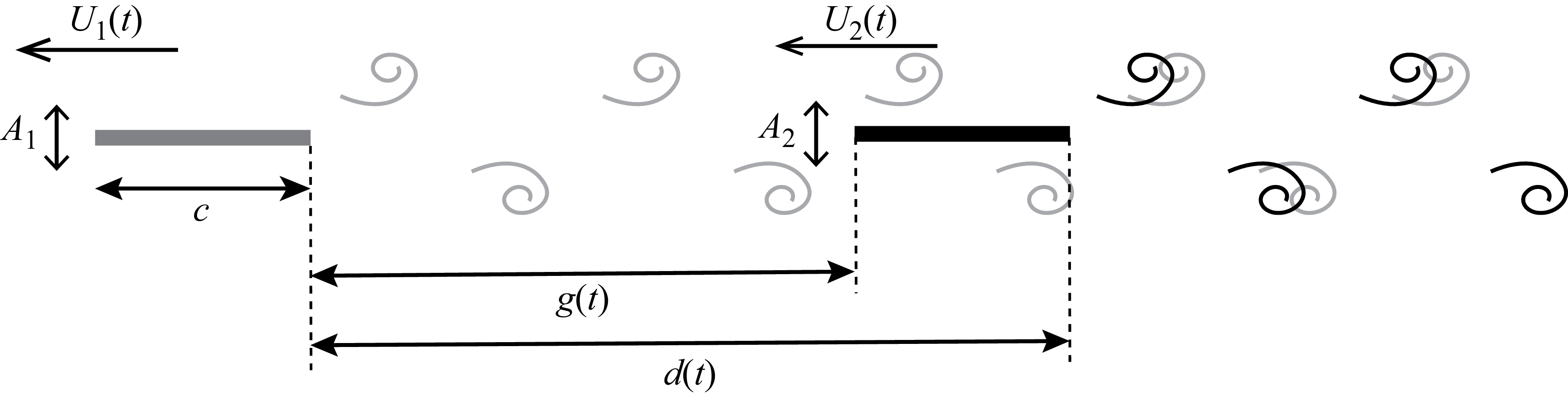


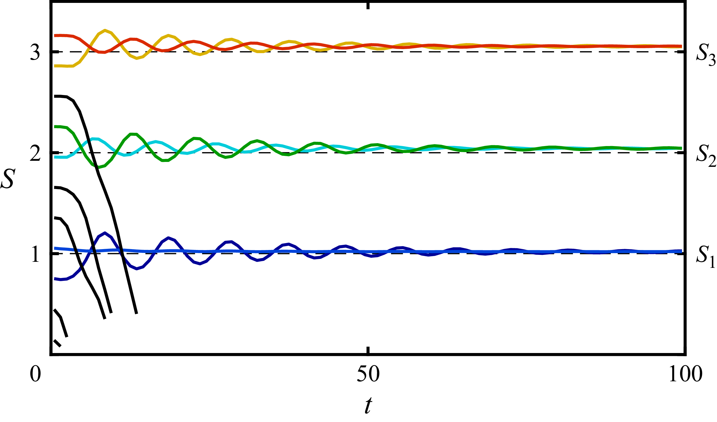


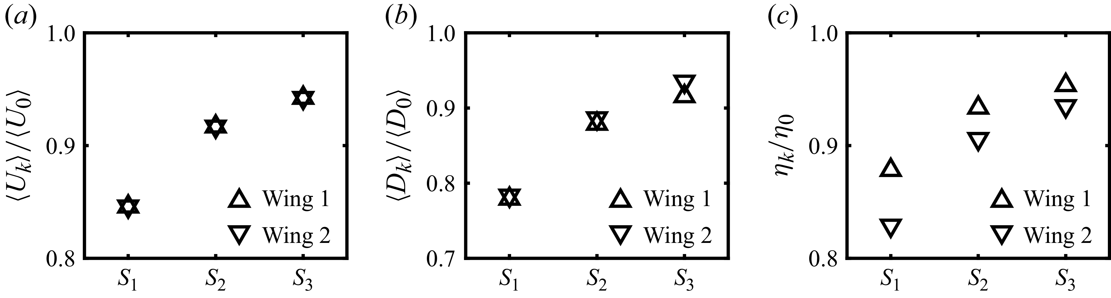


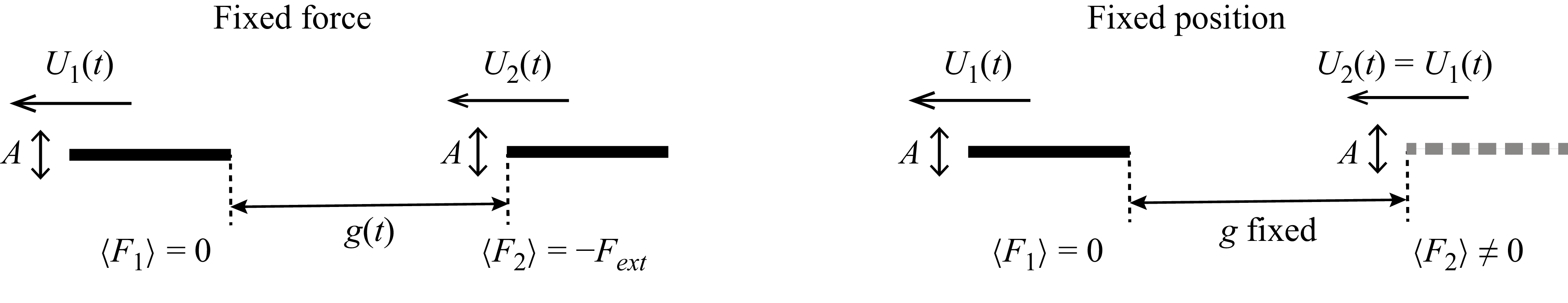


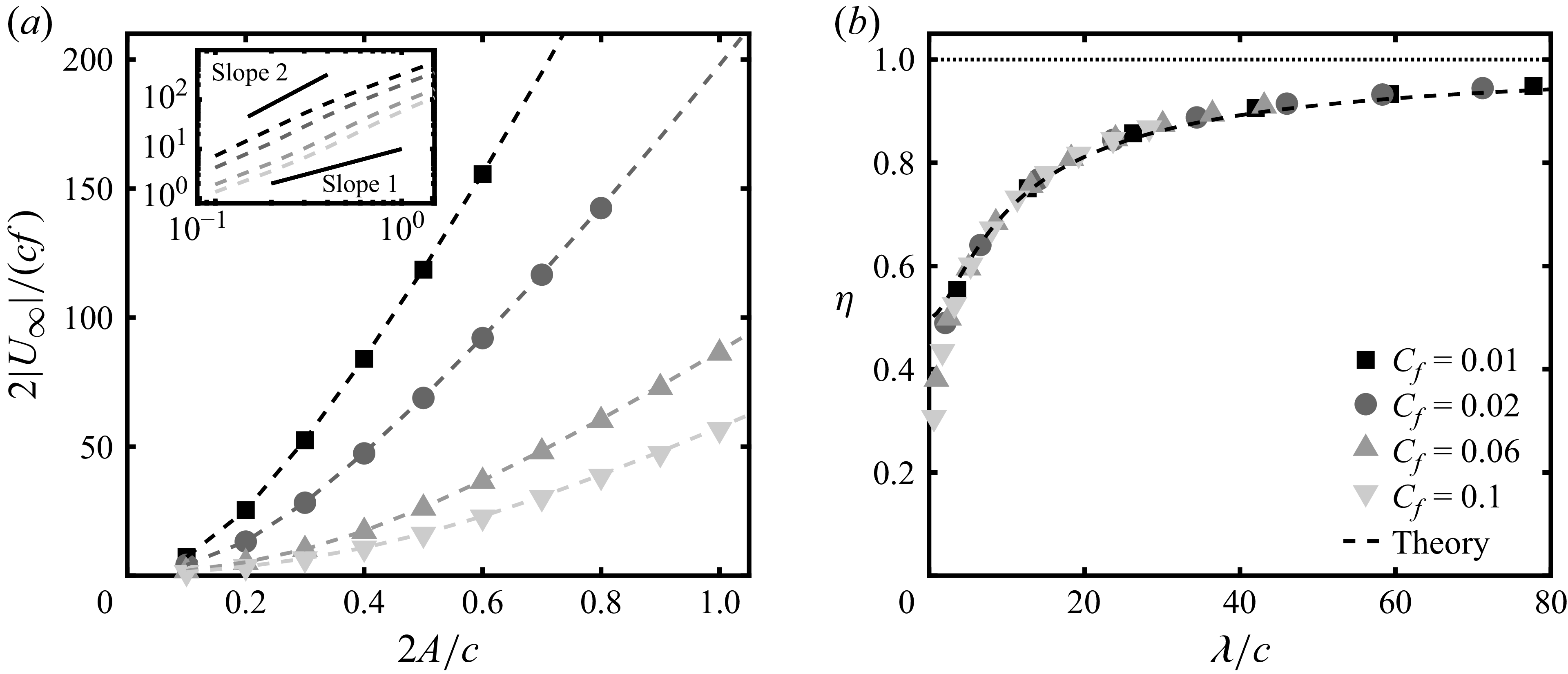


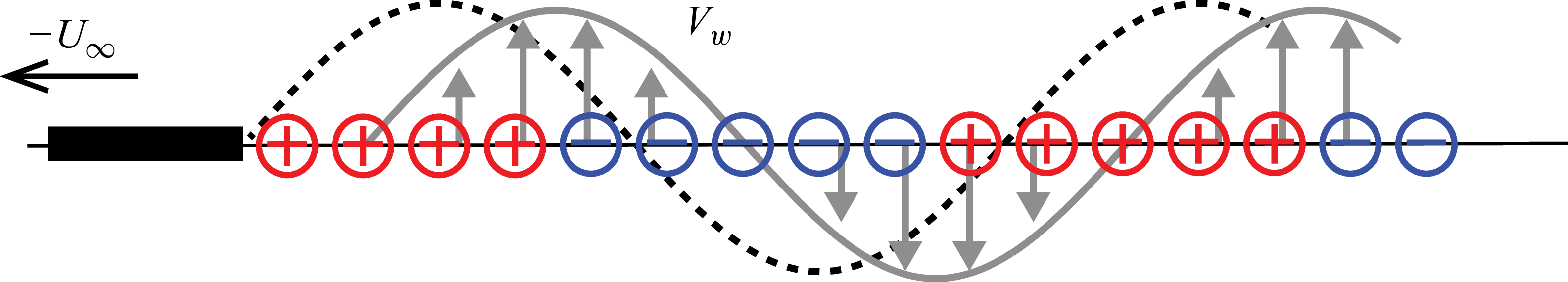


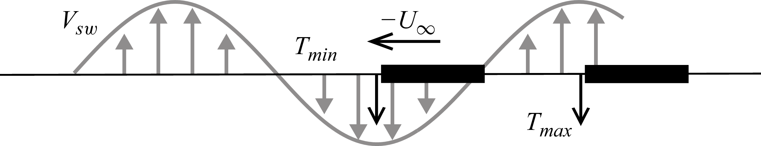


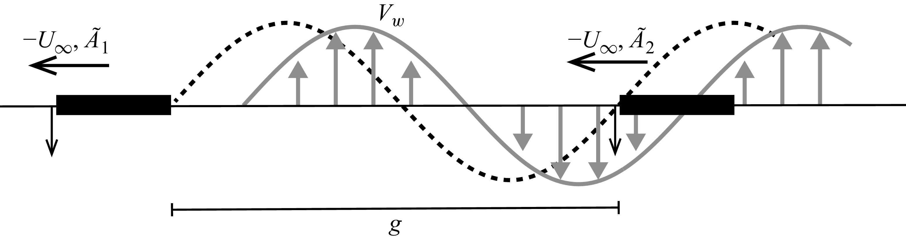


 Open access