2.1. Approach

The incompressible Navier–Stokes equations are non-dimensionalized with friction velocity $u_\tau$ and outer length scale, $h$, corresponding to a half-channel height. The friction velocity is the relevant near-wall velocity scale in the region of the logarithmic layer which will be the focus of subsequent analysis. Following Reynolds & Hussain (Reference Reynolds and Hussain1972), we then decompose the flow field, described by the velocity $u_i$ and kinematic pressure $p$, into the mean $\overline {(\;)}$, isolated single scale $\widetilde {(\;)}$ and remaining turbulent $(\;)'$ components

(2.1a,b)\begin{equation} u_i = \bar{u}_i + \tilde{u}_i + u_i', \quad p = \bar{p} + \tilde{p} + p'. \end{equation}

Here, the isolated scale consists of a single turbulent scale and all other remaining turbulent activity is lumped into $u_i'$. Such a decomposition is most easily conceptualized by invoking a narrow bandpass spectral filter around the wavenumber $\boldsymbol {k}_{\boldsymbol {f}}$; in this case the scale is cleanly defined in a spectral sense, but requires careful connection to observed very-large-scale motion. Here, we will adopt the simple narrow bandpass Fourier mode representation, but we argue later in § 3.1 that this is sufficient for explaining the observed amplitude modulation coefficient and the underlying phase relationships. Thus, $\tilde {u}_i$ comprises modes with wavenumber $\boldsymbol {k}_{\boldsymbol {f}}$ while $u_i'$ comprises modes with wavenumbers other than $\boldsymbol {k}_{\boldsymbol {f}}$. In what follows, we will define $\boldsymbol {k}_{\boldsymbol {f}}=(k_x,k_z,\omega )$, where $k_x$ and $k_z$ are real wavenumbers in the two spatial (wall-parallel) directions and $\omega$ is the real angular frequency, effectively a single scale in a triple Fourier decomposition. Substituting (2.1a,b) into the Navier–Stokes equations, that is,

(2.2a,b)\begin{equation} \frac{\partial u_i}{\partial t} + u_j \frac{\partial u_i}{\partial x_j} ={-} \frac{\partial p}{\partial x_i} + \frac{1}{{Re}} \frac{\partial^2 u_i}{\partial x_j^2}, \quad \frac{\partial u_i}{\partial x_i} = 0, \end{equation}

where ${Re} \equiv {u_\tau h}/{\nu }$ and $\nu$ is the kinematic viscosity, and then applying the narrow bandpass filter at $\boldsymbol {k}_{\boldsymbol {f}}$, we obtain the dynamical equation for the isolated-scale motion at $\boldsymbol {k}_{\boldsymbol {f}}$

(2.3a,b)\begin{equation} \frac{\partial \tilde{u}_i}{\partial t} + \bar{u}_j\frac{\partial \tilde{u}_i}{\partial x_j} + \tilde{u}_j\frac{\partial \bar{u}_i}{\partial x_j} + \frac{\partial \tilde{p}}{\partial x_i} - \frac{1}{{Re}} \frac{\partial^2 \tilde{u}_i}{\partial x_j^2} ={-} \frac{\partial \tilde{r}_{ij}}{\partial x_j} \equiv {\tilde{f}_i}, \quad \frac{\partial \tilde{u}_i}{\partial x_i} = 0, \end{equation}

where $\tilde {r}_{ij} = \widetilde {u_i' u_j'}$, the filtered fluctuation of the background mean stress, $\bar {r}_{ij} = \overline {u_i' u_j'}$, at the isolated scale (i.e. with wavenumber $\boldsymbol {k}_{\boldsymbol {f}}$), with contributions from fluctuations with $\boldsymbol {k}\ne \boldsymbol {k}_{\boldsymbol {f}}$. The dynamical equation for $\tilde {r}_{ij}$ (see Reynolds & Hussain Reference Reynolds and Hussain1972) is

(2.4a)\begin{equation} \frac{\partial \tilde{r}_{ij}}{\partial t} + \bar{u}_k \frac{\partial \tilde{r}_{ij}}{\partial x_k} + \tilde{u}_k \frac{\partial \bar{r}_{ij}}{\partial x_k} + \tilde{r}_{jk} \frac{\partial \bar{u}_i}{\partial x_k} + \tilde{r}_{ik} \frac{\partial \bar{u}_j}{\partial x_k} + \bar{r}_{jk} \frac{\partial \tilde{u}_i}{\partial x_k} + \bar{r}_{ik} \frac{\partial \tilde{u}_j}{\partial x_k} - \frac{1}{{Re}}\frac{\partial^2 \tilde{r}_{ij}}{\partial x_k^2} = \tilde{g}_{ij}, \end{equation}

where

(2.4b)\begin{equation} \tilde{g}_{ij} ={-} \frac{\partial }{\partial x_k} \widetilde{u_i' u_j' u_k'}\, {-} \widetilde{\phantom{0}u_j^{\prime}\frac{\partial {p^{\prime}}}{\partial x_i}\phantom{0}} {-} \widetilde{\phantom{0}u_i'\frac{\partial {p'}}{\partial x_j}\phantom{0}} {-} \frac{2}{{Re}} \widetilde{\frac{\partial {u}_i'}{\partial x_k}\frac{\partial {u}_j'}{\partial x_k}}. \end{equation}

Note the slight difference between the equivalent phase-averaged results of Reynolds & Hussain (Reference Reynolds and Hussain1972) and the effective Fourier decomposition of (2.3) and (2.4), namely, that the difference and product terms, i.e. the mean and $2\boldsymbol {k}_{\boldsymbol {f}}$ contributions, arising from phase averaging do not appear here as only the fluctuations at a single scale are being considered. The left-hand side of (2.4a) contains only linear terms, but the unclosed terms on the right renders it intractable for analysing the interaction between the isolated-scale motion $\tilde {u}_i$ and stress fluctuation $\tilde {r}_{ij}$ at first glance.

The linear operator containing the mean turbulent velocity profile in (2.3), the resolvent, describes many essential features of wall turbulence, including very-large-scale motion. In so-called resolvent analysis, the right-hand side, $\tilde {f}_i$, is modelled as an external forcing to the linear operator at each $\boldsymbol {k}_{\boldsymbol {f}}=(k_x,k_z,\omega )$ combination. The linear operator then responds to the forcing by preferentially amplifying certain modes above others. The most amplified (first) of these ‘velocity response modes’, or the mode most receptive to disturbances, as identified using the gain-based singular value decomposition, are then interpreted to be the likely candidates for turbulent motion observed in nature. For the sake of brevity, the reader is referred to McKeon (Reference McKeon2017) for details of the full formulation of the resolvent analysis. Channel flow is selected because the formulation for a fully developed flow is simpler than for a spatially growing (or locally parallel) turbulent boundary layer, although we also make a comparison with turbulent boundary-layer results, internal versus external flow boundary condition considerations notwithstanding.

Extending the original resolvent analysis, we wish to consider the interaction between a given energetic motion and stress fluctuation at the same scale by augmenting the linear operator for $\tilde {u}_i$, (2.3a,b), with the linear operator for $\tilde {r}_{ij}$, (2.4a). Relative to the approach of McKeon & Sharma (Reference McKeon and Sharma2010), this constitutes adding an equation to supply the appropriate structure for $\tilde {f}_i$. In the same vein, we model the nonlinear and unclosed terms $\tilde {g}_{ij}$ as external forcing. Owing to the increased complexity of this proposed approach, it seems prudent to first consider a simpler version of the scale interaction equations, namely by setting $\tilde {g}_{ij} = 0$. In effect, this can be considered as retaining only the part of $\tilde {r}_{ij}$ that is directly coupled to $\tilde {u}_i$; the part of $\tilde {r}_{ij}$ that responds to $\tilde {g}_{ij}$ is treated as uncorrelated to $\tilde {u}_i$ and therefore vanishes when joint statistics with $\tilde {u}_i$ are taken. Further manipulation of terms 2–4 in $\tilde {g}_{ij}$ is likely to result in their expression in terms of $\tilde {r}_{ij}$, particularly in light of the Biot–Savart relationship and the characterization of the pressure associated with each response mode by Luhar, Sharma & McKeon (Reference Luhar, Sharma and McKeon2014), which was shown to constitute the fast pressure, or that part of the pressure that is directly correlated with the mode velocity field, and the observations of amplitude modulation of the dissipation, the last term in $\tilde {g}_{ij}$, by Guala, Metzger & McKeon (Reference Guala, Metzger and McKeon2011). However, this is beyond the scope of the current problem. We focus on this simplified problem with a view to demonstrating the origin of the amplitude modulation of the small scales by the large scales described in § 1.

Our approach is to formulate and analyse the transfer function between the isolated scale and small-scale stress implied by (2.4a). In § 3, we formulate the transfer function between the analytically inspired modal formulations of small-scale stresses and isolated scales in the vicinity of a critical layer, and determine the phase difference between the two modes. In light of the agreement between our analysis and observations, we extend the modelling approach to make predictions concerning the relationship between very-large-scale motions and small-scale stress in the logarithmic region of the mean velocity in § 4.

2.2. Set-up for wall turbulence

Although formally applicable only for channel flows, the following analysis can also be extended to pipe and boundary-layer flows under the parallel flow assumption. A comparison between flows is likely to be most valid in the near-wall log and viscous regions, that is, where differences in flow geometry are negligible. We specialize the linear system, (2.4a) with $\tilde {g}_{ij} = 0$, to wall turbulence

(2.5a,b)\begin{equation} \bar{u} = \bar{u}(y), \quad \{\bar{v}, \bar{w}\} = 0, \end{equation}

where $x$, $y$ and $z$ or $u$, $v$ and $w$ are the streamwise, wall-normal and spanwise coordinates or velocities. The mean stresses generated by the fluctuating scales are given by

(2.6a,b)\begin{equation} \{\bar{r}_{xx},\bar{r}_{yy},\bar{r}_{zz}, \bar{r}_{xy}\}= \{\bar{r}_{xx},\bar{r}_{yy},\bar{r}_{zz}, \bar{r}_{xy}\}(y), \quad \{\bar{r}_{xz},\bar{r}_{yz}\} = 0; \end{equation}

the zeroes are from statistical symmetry. Velocity and stress fluctuations at the scale of interest are written as

(2.7)\begin{equation} \{\tilde{u}_i, \tilde{r}_{ij}\}(x,y,z,t) = \{\tilde{U}_i, \tilde{R}_{ij}\}(y;k_x,k_z,\omega) \exp({\mathrm{i}(k_x x + k_z z - \omega t)})+ \textrm{c.c}., \end{equation}

where the complex $\tilde {U}_i$ and $\tilde {R}_{ij}$ can be written in terms of a magnitude and phase as $\tilde {U}_i = |\tilde {U}_i| \,\textrm {e}^{\textrm {i} \phi _{U_i}}$ and $\tilde {R}_{ij} = |\tilde {R}_{ij}| \,\textrm {e}^{\textrm {i} \phi _{R_{ij}}}$, and $\textrm {c.c.}$ represents the complex conjugate of the preceding terms.

In this work, we focus our attention on (2.4a). Substituting (2.5a,b), (2.6a,b) and (2.7) in (2.4a), we obtain for each $(k_x,k_z,\omega )$,

(2.8a)\begin{equation} \boldsymbol{\mathsf{A}}\boldsymbol{\mathsf{R}}+\boldsymbol{\mathsf{B}}\boldsymbol{\mathsf{U}} = 0, \end{equation}

where

(2.8b)\begin{align} \boldsymbol{\mathsf{A}} &= \mathrm{i}(-\omega + k_x \bar{u}) \begin{bmatrix} 1 & 0 & 0 & 2\gamma & 0 & 0\\ 0 & 1 & 0 & 0 & 0 & 0 \\ 0 & 0 & 1 & 0 & 0 & 0 \\ 0 & \gamma & 0 & 1 & 0 & 0 \\ 0 & 0 & 0 & 0 & 1 & \gamma \\ 0 & 0 & 0 & 0 & 0 & 1 \end{bmatrix} - {Re}^{{-}1}(\mathrm{d}^2-k^2)\boldsymbol{\mathsf{I}}; \quad \boldsymbol{\mathsf{R}} =\begin{bmatrix} \tilde{R}_{xx} \\ \tilde{R}_{yy} \\ \tilde{R}_{zz} \\ \tilde{R}_{xy} \\ \tilde{R}_{xz} \\ \tilde{R}_{yz} \end{bmatrix}; \end{align}

(2.8c)\begin{align} \boldsymbol{\mathsf{B}} &= \begin{bmatrix} 2\bar{r}_{xx}\mathrm{i}k_x + 2\bar{r}_{xy}\,\mathrm{d} & \bar{r}_{xx,y} & 0\\ 0 & \bar{r}_{yy,y} + 2 \bar{r}_{xy} \mathrm{i} k_x + 2 \bar{r}_{yy} \,\mathrm{d} & 0\\ 0 & \bar{r}_{zz,y} & 2\bar{r}_{zz}\mathrm{i}k_z\\ \bar{r}_{xy} \mathrm{i} k_x + \bar{r}_{yy}\,\mathrm{d} & \bar{r}_{xy,y} + \bar{r}_{xx} \mathrm{i} k_x + \bar{r}_{xy} \,\mathrm{d} & 0\\ \bar{r}_{zz} \mathrm{i} k_z & 0 & \bar{r}_{xx} \mathrm{i} k_x + \bar{r}_{xy} \,\mathrm{d}\\ 0 & \bar{r}_{zz} \mathrm{i} k_z & \bar{r}_{xy} \mathrm{i}k_x + \bar{r}_{yy} \,\mathrm{d} \end{bmatrix}; \quad \boldsymbol{\mathsf{U}} = \begin{bmatrix} \tilde{U} \\ \tilde{V} \\ \tilde{W} \end{bmatrix}; \end{align}

$\gamma =(\mathrm {d}\bar {u}/\mathrm {d} y)/[\mathrm {i}(-\omega + k_x\bar {u})]$; $\overline {(\;)}_{,y} \equiv \mathrm {d}\overline {(\;)}/\mathrm {d} y$; $\mathrm {d} \equiv \mathrm {d}/\mathrm {d} y$; $k^2 = k_x^2 + k_z^2$; and $\boldsymbol{\mathsf{I}}$ is the identity matrix. The denominator of $\gamma$ has special significance in the vicinity of a critical layer, i.e. the wall-normal location, $y_c$, where the streamwise propagation velocity of a motion of scale $\boldsymbol {k}_f$ is equal to the local mean velocity,

(2.9)\begin{equation} -\omega + k_{x} \bar{u}(y_{c}) \equiv 0 \quad \textrm{such that} \ \begin{cases} \bar{u} < \omega/k_{x} & \textrm{if} \ y < y_{c}, \\ \bar{u} = \omega/k_{x} & \textrm{if} \ y = y_{c}, \\ \bar{u} > \omega/k_{x} & \textrm{if} \ y > y_{c}. \end{cases}\end{equation}

Given $k_x$ and $k_z$, one could, in principle, discretize $\mathrm {d}$ and insert $\tilde {U}_i$ and $\omega$ from an earlier analysis (e.g. McKeon & Sharma Reference McKeon and Sharma2010) to obtain the response $\tilde {R}_{ij}$. However, unlike the earlier analysis of the velocities, the discretization of $\boldsymbol{\mathsf{B}}$ involves measuring or approximating all of the average Reynolds stresses, $\bar {r}_{ij}$, also. Because it is not clear how sensitive the relationship between $\boldsymbol{\mathsf{U}}$ and $\boldsymbol{\mathsf{R}}$ is to the details of the Reynolds stresses, we approach the problem analytically, in order to draw conclusions based on a minimum of empirical measurements while also establishing the extent to which detailed measurements may be important for any future, discretized analysis. Here, we examine the implications of the analytical transfer function between $\boldsymbol{\mathsf{R}}$ and $\boldsymbol{\mathsf{U}}$ of (2.8) by employing a semi-analytical form for the first resolvent modes. In particular, we focus our effort on the relationship between the streamwise velocity components, which have been the topic of extended study through experimental observations in canonical wall turbulence, and seek to identify the transfer function between the isolated scale $\tilde {U}$ and corresponding fluctuating streamwise stress, $\tilde {R}_{xx}$. Introducing a relative phase between $\tilde {R}_{xx} \equiv \tilde {R}_{11}$ and $\tilde {U} \equiv \tilde {U}_1$,

(2.10)\begin{equation} \frac{\tilde{R}_{xx}(y)}{\tilde{U}(y)}=\frac{|\tilde{R}_{xx}(y)|}{|\tilde{U}(y)|} \,\textrm{e}^{{\mathrm{i}} \varphi(y)}, \end{equation}

where $\varphi \equiv \arg \tilde {R}_{xx} - \arg \tilde {U} = \arg (\tilde {R}_{xx}\tilde {U}^*) \equiv \phi _{{R}} - \phi _{U}$, where $\ast$ denotes the complex conjugate. Note that the relative phase $\varphi$ is defined with respect to the spatial variables such that it has the opposite sense to the phase described relative to the temporal domain in e.g. Jacobi & McKeon (Reference Jacobi and McKeon2013).

2.3. Very-large-scale motion as the isolated scale, $\tilde{U}$

We consider a three-dimensional isolated scale that is representative of the structure of a VLSM and turn our attention to scale interactions occurring in the log region of wall turbulence. Observations of VLSMs in the literature (e.g. Hutchins & Marusic Reference Hutchins and Marusic2007; Chung & McKeon Reference Chung and McKeon2010; Hutchins et al. Reference Hutchins, Monty, Ganapathisubramani, Ng and Marusic2011) have identified the appropriate streamwise and spanwise wavenumbers to be $k_x \approx 1$ and $k_z \approx \pm 6$, corresponding to wavelengths of approximately six and one times the outer length scale, respectively, and a structure convecting in the $x$-direction. The appropriate frequency (or, equivalently, convection velocity) can be determined with reference to the channel flow results of Mathis et al. (Reference Mathis, Monty, Hutchins and Marusic2009b) at ${\textit {Re}}_\tau = 3000$. The locus of the outer (large scale) peak energy has been identified as corresponding to $y = 3.9{\textit {Re}}_\tau ^{-1/2}$, although there remains some uncertainty about this particular form (see Vallikivi, Ganapathisubramani & Smits Reference Vallikivi, Ganapathisubramani and Smits2015). McKeon & Sharma (Reference McKeon and Sharma2010) have discussed the effectiveness of a single resolvent mode as a proxy for the real VLSM; extending this approach, the location of the outer peak energy corresponds to the VLSM critical layer, such that the convection velocity is given by the local mean velocity at this wall-normal location.

2.4. Phase relationship between the streamwise velocity of the isolated scale and corresponding fluctuating stress via correlation coefficients

The phase relationship between the streamwise component of the isolated scale, $\tilde {u}$, and the stress fluctuation at the same isolated scale, $\tilde {r}_{xx}$, can also be characterized using experimental or numerical observations and a direct correlation coefficient (Duvvuri & McKeon Reference Duvvuri and McKeon2015; Jacobi & McKeon Reference Jacobi and McKeon2017)

(2.11)\begin{equation} {\varPhi(y) = \frac{\left\langle \tilde{u}\, \tilde{r}_{xx} \right\rangle}{\left\langle (\tilde{u})^2 \right\rangle^{1/2} \left\langle (\tilde{r}_{xx})^2 \right\rangle^{1/2}}{,} } \end{equation}

where $\langle \,\rangle$ is the inner product. It can then be shown that

(2.12)\begin{equation} {\varPhi=\cos\mathcal{\varphi}}, \end{equation}

that is, $\varPhi$ is directly related to the relative phase between $\tilde {R}_{xx}$ and $\tilde {U}$ (2.10). It does not contain explicit information about their relative magnitudes due to the normalization, nor the sense of the phase relationship due to the symmetry of the cosine function.

The more common amplitude modulation coefficient, $\mathcal {R}$, was derived (e.g. Bandyopadhyay & Hussain Reference Bandyopadhyay and Hussain1984; Mathis et al. Reference Mathis, Hutchins and Marusic2009a) in terms of the correlation between a large-scale signal, $u_L$, defined using a filter in wavenumber space at $k_{x}=k_{\zeta }$, where

(2.13)\begin{equation} u(y,t)=u_L(y,t)+u_S(y,t), \end{equation}

and the envelope, $\mathcal {E}_L$, of the small-scale turbulence signal, $u_S$, filtered at the same wavenumber, i.e.

(2.14)\begin{equation} \mathcal{R} = \frac{\left\langle u_L \mathcal{E}_L\right\rangle}{\left\langle u_L^2 \right\rangle^{1/2} \left\langle \mathcal{E}_L^2 \right\rangle^{1/2}}. \end{equation}

Section 4 describes the relationship between $\mathcal {R}$, the stress fluctuation $\tilde {r}_{xx}$ and the isolated scale $\tilde {u}$, and argues that the isolated-scale and the stress-fluctuation terms are representative of the envelopes of large- and small-scale fluctuations. Therefore, the analysis here in terms of $\tilde {U}$ and $\tilde {R}_{xx}$ is relevant also to the filtered, amplitude modulation analysis.

Qualitatively, correlation coefficients such as $\varPhi$ and $\mathcal {R}$ can be interpreted in terms of triadically consistent scales: non-zero contributions arise only from stress fluctuations at the wavenumber of the isolated scale in $\varPhi$, or from small-scale stress fluctuations associated with the entire spectral content of the large-scale velocity signal, $u_L$, in $\mathcal {R}$. To reiterate, then, the direct correlation coefficient, $\varPhi$, describes the relationship between the isolated scale and that portion of the stress fluctuation $r_{xx}$ that is triadically consistent with $\tilde {U}$, namely $\tilde {R}_{xx}$. By contrast, the amplitude modulation coefficient considers only the small-scale stress component that is triadically consistent with the entire spectral content of the large-scale signal, $u_L$. A formal description of this interpretation is given in Duvvuri & McKeon (Reference Duvvuri and McKeon2015).

3.1. Transfer function including viscous effects

Our ultimate goal is the investigation of the amplitude modulation effect in canonical wall turbulence. This has been shown to be dominated by the VLSM (Jacobi & McKeon Reference Jacobi and McKeon2013), i.e. we will later hypothesize that the VLSM can be modelled by an isolated scale in this analysis. However, we begin by considering the scale interactions corresponding to a single, truly isolated very large scale. We focus our effort on the relationship between streamwise velocity components, which has been the topic of extended study through experimental observations in canonical wall turbulence, and identify the transfer function between the isolated scale, ${\tilde {U}}$, and corresponding fluctuating streamwise stress, ${\tilde {R}_{xx}}$. The transfer function indicates the relative magnitudes and phases between the isolated scale and fluctuating stresses. In general, the phase difference between two scales can be used to reconstruct the relative spatial orientation between them. If the orientation of an isolated, large-scale motion, i.e. its downstream inclination angle, is known, then the phase difference between that large-scale and another scale indicates the relative inclination of the second scale with respect to the first. Here, the transfer function can provide a picture of the relative spatial orientation of these large-scale motions and fluctuating stress in wall-bounded flows.

Because the structure of the large-scale motions is hypothesized to be intrinsically connected to the location of the critical layer for VLSMs, where the outer energy peak is observed in premultiplied spectral maps, we focus the transfer function analysis on VLSMs in the spatial vicinity of their critical layer.

The critical layer is the viscous region of flow that resolves the singularity in the inviscid Rayleigh equation which occurs when the phase speed of a neutrally stable velocity mode equals the local mean convection velocity of the flow in which it propagates. The viscous critical layer behaviour applies to small amplitude velocity modes; for large amplitude disturbances, nonlinear critical behaviour can resolve the singularity in the absence of viscosity, as detailed in Haberman (Reference Haberman1976). Therefore, we must assume that the nonlinear forcing contained in the $\tilde {f}_i$ term in (2.3) is small. Lin (Reference Lin1955) showed through asymptotic analysis that the thickness of the linear critical layer, $\epsilon$, scales as $(k_x {Re} )^{-1/3}$, thus approaching zero as $(k_x {Re}) \to \infty$. For convenience, we include the local velocity gradient at the critical point, $\mathrm {d}\bar {u}_c$, in the definition of the critical layer thickness

(3.1)\begin{equation} \epsilon = \left(k_x \,\mathrm{d}\bar{u}_c {Re} \right)^{{-}1/3}. \end{equation}

For large wavelength velocity modes, the critical layer forms a distinct region of the flow, separate from the viscous wall layer.

However, because viscosity is not negligible in the critical layer, the Reynolds number dependent terms in (2.8b) must be preserved, which means the $\boldsymbol{\mathsf{A}}$ matrix operator acting on the $\tilde {R}_{ij}$ terms is invertible upon discretization of the $\mathrm {d}$ operator, but no simple transfer function between arbitrary $\tilde {U}$ and $\tilde {R}_{ij}$ can be determined analytically. In order to obtain a transfer function applicable in the vicinity of the viscous critical layer, we must therefore assume that the functional form of the stress fluctuations, $\tilde {R}_{ij}$, is modal.

In order to approximate a modal representation of the stress fluctuations, we begin with the representation of a single, isolated velocity scale. One such representation is given in the work of Dawson & McKeon (Reference Dawson and McKeon2019), who showed that the leading streamwise modes associated with the incompressible Navier–Stokes resolvent operator can be approximated in analytical form, in the limit of long wavelength disturbances, $k \ll 1$ (using the outer non-dimensionalization), as

(3.2)\begin{equation} \tilde{U} = M_U \exp{\left[ -\textrm{i} \alpha_U \frac{ (y-y_m)}{\epsilon} - \beta_U \left(\frac{y-y_m}{\epsilon}\right)^2 \right]}, \end{equation}

for positive, $ {O}(1)$ coefficients $\alpha _U=\alpha _U(k_z,k_z)$ and $\beta _U=\beta _U(k_z,k_z)$ that depend on the streamwise wavenumber $k_x$ and the wall-parallel wavenumber magnitude $k$, with $M_U = M_U(k_x,k_z)$ the amplitude of the mode peak; $y_m$ denotes the location of the modal maximum, dictated by the wave speed of the mode, $\omega /k_x$. The asymptotic form of (3.2) consists of a Gaussian profile whose width scales with the size of the critical layer, $\epsilon$. This general model was shown to be quite robust, applying over an unexpectedly large range of streamwise wavenumbers, especially in the vicinity of the critical layer itself. However, the model was not formally developed to describe the wall-normal velocity component, which is needed here for formulating the fluctuating stresses, and thus further assumptions will be necessary for this component. Other models are also possible; the work of Dawson & McKeon (Reference Dawson and McKeon2019) is used by way of example. The validity of the following analysis depends on this particular choice of model only insofar as the length scales associated with the mode shapes scale on the critical layer thickness, $\epsilon$.

The fluctuating stress, $\tilde {R}_{ij}$, associated with the specific triadic interaction that includes the isolated large scale, $\tilde {U}$, can be constructed by multiplication of the two remaining members of that triad, each obtained from a distinct, narrow, band-pass filter of the governing equations. For the streamwise, normal Reynolds stress, we simply multiply two instances of the Gaussian model in (3.2), which results in another Gaussian model for the stress with $i=j=x$

(3.3)\begin{equation} \tilde{R}_{ij} = M_{ij} \exp{\left[ -\textrm{i} \alpha_{ij} \frac{ (y-y_{m,ij})}{\epsilon} - \beta_{ij} \left(\frac{y-y_{m,ij}}{\epsilon}\right)^2 \right]}, \end{equation}

where the coefficients $\alpha _{ij}=\alpha _{ij}(k_x,k_z)$ and $\beta _{ij}=\beta _{ij}(k_x,k_z)$ reflect the width and phase variations of the resulting stress, which depend on the triadic composition of the two isolated mode wavenumbers through their respective values of $\alpha _U$ and $\beta _U$.

In order to construct the $\tilde {R}_{xy}$ and $\tilde {R}_{yy}$ fluctuating stresses, we need to first modify (3.2) to describe the wall-normal component, $\tilde {V}$. The primary distinguishing features of the wall-normal component are: (i) the lack of phase variation across the region of the critical layer, as discussed in more detail in § 3.2; and (ii) a taller Gaussian profile than the streamwise component. Therefore, we assume that $\alpha _V \approx 0$ and that the profile of $\tilde {V}$ can be approximated by a constant-phase Gaussian, at least in the vicinity of the critical layer, with $\beta _{V} < \beta _{U}$ to enforce a taller profile. Performing the same multiplication within the triad described above, $\tilde {R}_{xy}$ takes the same form as (3.3), since the phase variation represented by $\alpha _{xy}$ is preserved by the streamwise component, and $\tilde {R}_{yy}$ also takes that form but with $\alpha _{yy} \approx 0$, since neither wall-normal component includes phase variation, and also $\beta _{yy} < \beta _{xx}$.

We apply the formulation of $\tilde {R}_{ij}$ in (3.3) to show that when the viscous part of the $\boldsymbol{\mathsf{A}}$ matrix operator acts on $\tilde {R}_{ij}$, the result is simply proportional to $\tilde {R}_{ij}$ itself, i.e.

(3.4)\begin{equation} {-}(\mathrm{d}^2-k^2) \tilde{R}_{ij} = \underbrace{\left[k^2 + 2 \frac{\beta_{ij}}{\epsilon^2} + \left(\frac{\alpha_{ij}}{\epsilon} - \textrm{i}\frac{2 \beta_{ij}}{\epsilon^2} (y-y_{m,ij}) \right)^2 \right]}_\text{$\ell_{ij}^{{-}2}(y)$}\tilde{R}_{ij}, \end{equation}

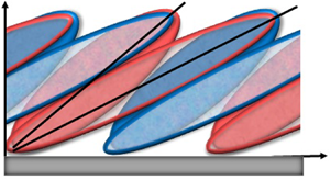
where we define a wavenumber-dependent length scale $\ell _{ij}$ to represent the local radius of curvature of the stress profile. See figure 1 for a sketch of the physical representation of the isolated mode and stress, which identifies the relationship between, for example, $\phi _U$ and $\alpha _U$.

Figure 1.

A schematic of the relevant length scales associated with the large- and small-scale motions in the vicinity of the critical layer. (a) The streamwise component of the isolated large-scale mode can be represented by (3.2), with mode width $\beta _U$ and phase slope, near its centre $y_m$ of $-\alpha _U/\epsilon$, resulting in a downstream inclination $\theta _U$. (b) The wall-normal component of the isolated large-scale mode. Here, the key assumption is that the phase variation across the critical layer, $\textrm {d}\phi _V$ is negligible and that ${\textrm {d}|\tilde {V}|}/{|\tilde {V}|} \lesssim k_x$. (c) The streamwise stress component, which can also be represented by (3.3). At the wall, the streamwise stress shares the same phase as the isolated large scale. At the critical layer, the large-scale phase is $0$ and the small-scale phase is $-{\rm \pi} /2$, such that $\varphi = \phi _R - \phi _U = -{\rm \pi} /2$, consistent with (3.14).

Substituting the modal form of the stress into the matrix operator $\boldsymbol{\mathsf{A}}$ renders the system analytically invertible and thus the transfer function is obtained by solving

(3.5)\begin{equation} \boldsymbol{\mathsf{R}}={-}\boldsymbol{\mathsf{A}}^{{-}1} \boldsymbol{\mathsf{BU}}, \end{equation}

to arrive at the direct relation between the streamwise component of stress, $\tilde {R}_{xx}$, and the large scale $\tilde {U}$. The full transfer function, written in terms of a general modal stress, is presented in appendix A, specifically (A3).

3.2. Simplified transfer function near the critical layer

The analytical transfer function, including viscosity, is then simplified by expanding it about a point $y$ in the vicinity of the critical point, $y_c$ (where the local mean velocity matches the wave speed, according to (2.9)), by writing

(3.6)\begin{equation} (-\omega + k_x \bar{u}) \approx k_x \,\mathrm{d}\bar{u}_c {\rm \Delta} y = \epsilon^{{-}3} {Re}^{{-}1} {\rm \Delta} y, \end{equation}

where $y = y_c + {\rm \Delta} y$, ${\rm \Delta} y / \epsilon \ll 1$ and the definition of the critical layer thickness, $\epsilon$, is given by (3.1). Substituting into $\gamma$, we obtain

(3.7)\begin{equation} \gamma = \frac{-\textrm{i} \, \mathrm{d} \bar{u}}{(-\omega + k_x\bar{u})} \approx \frac{-\textrm{i} \, \mathrm{d} \bar{u} }{k_x \,\mathrm{d}\bar{u}_c {\rm \Delta} y} \approx \frac{-\textrm{i}}{(k_x {\rm \Delta} y)} \frac{y_c}{y}, \end{equation}

where we assume that the velocity profile is logarithmic and thus $\mathrm {d} \bar {u} = 1/(\kappa y)$ and $\mathrm {d} \bar {u}_c = 1/(\kappa y_c)$, where $\kappa$ is the von Kármán constant. ($\mathrm {d} \bar {u}$ can also be evaluated at the critical layer itself, but we retain the $y$-dependence for generality.)

Near the critical layer, we also neglect the $y$-dependence in the stress curvature length scale, $\ell _{ij}$, by assuming that the critical layer occurs near the peak of the fluctuating stress profile. For the streamwise, normal and shear stresses, this means ${\mathrm {d}|\tilde {R}_{ij}|}/{|\tilde {R}_{ij}|} \ll |\mathrm {d}\phi _{R_{ij}}|$. Using the analytical model in (3.3), this assumption is equivalent to the claim that the distance between the critical layer and the modal maximum is much smaller than the layer itself, i.e. $|y_c - y_{m,ij}|/\epsilon \ll \alpha _{ij}/(2 \beta _{ij})$, where $\Delta y$ is assumed arbitrarily small, for simplicity. For $\tilde {R}_{yy}$, where $\alpha _{yy} \approx 0$, we assume instead that $|y_c - y_{m,yy}|/\epsilon \ll \sqrt {1/(2 \beta _{yy})}$. Because $\beta _{yy} < \beta _{xx}$, this assumption implies that the distance between the centre of $\tilde {R}_{yy}$ and the critical layer may be greater than in the case of $\tilde {R}_{xx}$. Applying these assumptions about $\ell _{ij}$, we eliminate the final term in the square brackets of (3.4) and the radius of curvature reduces to

(3.8)\begin{equation} \ell_{ij}^{2} = \frac{\epsilon^2 }{(k \epsilon)^2 + 2 \beta_{ij} + \alpha_{ij}^2 }, \end{equation}

where $\ell _{ij} > 0$ is now real. Assuming that $(k \epsilon )$ is small at high Reynolds number (i.e. $k_z \epsilon \ll 1$ for small $k_x$) and that the stress modes scale on the critical layer thickness, such that the $\alpha _{ij}$ and $\beta _{ij}$ parameters are $ {O}(1)$, then $\ell _{ij} \propto \epsilon$.

The resulting transfer function still depends on three distinct modal scales, $\ell _{xx}$, $\ell _{xy}$ and $\ell _{yy}$, as shown in full in appendix A (A4). However, for algebraic simplicity, we assume that the $\ell _{ij}$ length scales are of similar magnitude and thus let $\ell _{xx} = \ell _{xy} = \ell _{yy} = \ell$, although this assumption can easily be relaxed. The analytical transfer function for the streamwise velocity components expanded in the vicinity of critical layer, is then

(3.9)\begin{align} &-\frac{1}{\epsilon^2 {Re}} \left[ \textrm{i}\frac{{\rm \Delta} y}{\epsilon} + \epsilon^2 \ell^{{-}2} \right] \tilde{R}_{xx} =\left[2 \text{i} k_x \bar{r}_{xx} + 2 \bar{r}_{xy} \,\mathrm{d} - \frac{2 \left( \dfrac{1}{k_x \epsilon} \right) \left( \dfrac{y_c}{y}\right) (\textrm{i} k_x \bar{r}_{xy} + \bar{r}_{yy}\,\mathrm{d}) }{ \textrm{i}\dfrac{{\rm \Delta} y}{\epsilon}+ \epsilon^2 \ell^{{-}2}} \right] \tilde{U} \nonumber\\ &\quad + \left[\bar{r}_{xx,y} - \frac{2 \left( \dfrac{1}{k_x \epsilon} \right) \dfrac{y_c}{y} (\textrm{i} k_x \bar{r}_{xx} + \bar{r}_{xy} \, \mathrm{d} + \bar{r}_{xy,y})}{\textrm{i}\dfrac{{\rm \Delta} y}{\epsilon}+ \epsilon^2 \ell^{{-}2}} + \frac{2 \left( \dfrac{1}{k_x \epsilon} \right)^2 \left( \dfrac{y_c}{y}\right)^2 (2 \textrm{i} k_x \bar{r}_{xy} + 2 \bar{r}_{yy} \,\mathrm{d} + \bar{r}_{yy,y})}{ \left[\textrm{i}\dfrac{{\rm \Delta} y}{\epsilon}+ \epsilon^2 \ell^{{-}2}\right] \left[\textrm{i}\dfrac{{\rm \Delta} y}{\epsilon}+ \epsilon^2 \ell^{{-}2}\right]}\right] \tilde{V}, \end{align}

where we observe that the streamwise stress depends on both streamwise and wall-normal large scales, and their spatial derivatives, whereas the experimental measurements typically report the connection between the streamwise components only. To simplify the analysis, we determine the conditions under which the $\tilde {V}$ contribution to the stress can be neglected, by comparing the dominant term in $\tilde {V}$ with the least dominant term in $\tilde {U}$, as elaborated in appendix A, resulting in four conditions

(3.10a)\begin{gather} \frac{k_x \bar{r}_{xx}}{\bar{r}_{yy,y}} \gtrsim 1, \end{gather}

(3.10b)\begin{gather}\frac{1}{k_x} \frac{\textrm{d}|\tilde{V}|}{ |\tilde{V}|} \lesssim 1, \end{gather}

(3.10c)\begin{gather}\tan{\theta_U} \lesssim \left|\frac{\bar{r}_{xy}}{\bar{r}_{xx}}\right|, \end{gather}

(3.10d)\begin{gather}\left| \frac{\tilde{V}}{\tilde{U}} \right| \ll (k_x \epsilon)^{2} \left|\frac{\bar{r}_{xx}}{\bar{r}_{xy}} \right|. \end{gather}

Condition (3.10a) indicates that the Reynolds stresses have negligible spatial variation in the vicinity of the critical layer, which is consistent with Townsend's equilibrium layer argument within the logarithmic region of the velocity profile. From the boundary-layer measurements of Jacobi & McKeon (Reference Jacobi and McKeon2013) at ${Re}_\tau = 910$, the ratio ${ \bar {r}_{xx}}/{ \bar {r}_{yy,y}} \approx 1.5$ near the critical layer, and thus this is satisfied for all $k_x \gtrsim 0.67$.

Condition (3.10b) indicates that the length scale associated with wall-normal changes in $\tilde {V}$ is no smaller than the wavelength of the isolated disturbance, which is already satisfied for most values of $k_x$ by the earlier assumption that the peak fluctuating stress occurs near the critical layer.

Condition (3.10c) depends on the large-scale inclination angle, $\theta _U$, and the ratio of the Reynolds stresses. The ratio of the Reynolds streamwise normal stress to other Reynolds stress components, $|{\bar {r}_{xx}}/{\bar {r}_{xy}} |$ or $|{\bar {r}_{xx}}/{\bar {r}_{yy}} |$, is typically $ {O}(10)$, as reported in Fernholz & Finley (Reference Fernholz and Finley1996). And the typical streamwise inclination angle, $\theta _U \approx 15^{\circ }$, as reported in Marusic & Heuer (Reference Marusic and Heuer2007), thus $\tan {\theta _U} \approx 0.27$, satisfying this requirement.

This leaves just the condition (3.10d) to enforce. Substituting the definition of $\epsilon$ and assuming that, in the logarithmic layer, $\textrm {d}\bar {u}_c \approx (\kappa y_c)^{-1}$ and $y_c \approx 3.9 {Re}^{-1/2}$, and again that $|{\bar {r}_{xx}}/{\bar {r}_{xy}} | \sim 10$, yields

(3.11)\begin{equation} \left| \frac{\tilde{V}}{\tilde{U}} \right| \ll 10 k_x^{4/3} {Re}^{{-}1}. \end{equation}

For $k_x = 1$ and ${Re} = 910$ (for later comparison with Jacobi & McKeon (Reference Jacobi and McKeon2013)), this means the ratio of wall-normal to streamwise modes must be less than approximately $0.01$, which is almost but not exactly satisfied in numerical calculations of the resolvent modes based on empirical mean velocity profiles, and in the forced modes observed in Jacobi & McKeon (Reference Jacobi and McKeon2017). Formally satisfying the requirement would require large scales of the order of three outer units, $k_x = 2{\rm \pi} /3$, with ${Re} \approx 1000$, or larger scales at still smaller Reynolds numbers. Note, however, that this requirement is met by definition for resolvent modes based on the Squire operator rather than the full Orr–Sommerfeld operator, as discussed, e.g. in Dawson & McKeon (Reference Dawson and McKeon2019). Therefore, we proceed with some caution in neglecting all of the terms pre-multiplying $\tilde {V}$ in (3.9) and presenting the analysis of the transfer function in terms of only the streamwise component, $\tilde {U}$.

The criteria for neglecting the $\tilde {V}$ contribution to the transfer function listed in (3.10) also implicitly relied on an additional assumption, that ${\textrm {d}|\tilde {U}|}/{|\tilde {U}|} \ll |\textrm {d}\phi _{U}|$, i.e. that the critical layer occurs very near the maximum in the isolated-scale mode shape. However, this is really the very same assumption we already applied above, with respect to the maximum in the stress profile, where we assumed that ${\textrm {d}|\tilde {R}_{xx}|}/{|\tilde {R}_{xx}|} \ll |\textrm {d}\phi _{R}|$. The result of this assumption is that the spatial derivatives $\textrm {d}\tilde {U}$ can be assumed to represent predominantly the variation in large-scale phase, $\textrm {d}\phi _U$ and not magnitude.

The simplified, streamwise transfer function is finally separated into real and imaginary parts, shown in detail in appendix A. A final simplifying assumption is applied to the transfer function: terms of $ {O}(k_x \epsilon )$ compared to the leading-order terms are neglected, to yield

(3.12)\begin{align} \frac{\tilde{R}_{xx}}{\tilde{U}} = \frac{\epsilon {Re} \left({-}2 \bar{r}_{xy} - 2 \bar{r}_{yy} \dfrac{\textrm{d}\phi_U}{k_x} \right) \left(\dfrac{y_c}{y}\right)}{\left[ \left(\dfrac{{\rm \Delta} y}{\epsilon} \right)^2 + \left( \frac{\epsilon}{\ell} \right)^4 \right]^2} \left\{{-}2\left(\frac{{\rm \Delta} y}{\epsilon} \right) \left(\frac{\epsilon}{\ell}\right)^2 + i \left( \left[ \left(\frac{{\rm \Delta} y}{\epsilon} \right)^2 - \left( \frac{\epsilon}{\ell} \right)^4 \right] \right) \right\}, \end{align}

where we assume that $d \phi _U < 0$ to represent downstream inclined structures and $\bar {r}_{xy} < 0$ following the usual convention for attached flows. Therefore, ${( -2 \bar {r}_{xy} - 2 \bar {r}_{yy} ({\textrm {d}\phi _U}/{k_x} )) > 0}$. All of the assumptions used in this simplified analysis and the more general treatment in the next section are summarized in table 1.

Table 1.

Definitions and assumptions made in the analysis of the transfer function. See figure 1 for a schematic view of the quantities involved.

The sense of the phase, $\varphi$, is determined by the sign of the imaginary part of the transfer function, which depends on the size of the region of interest, ${\rm \Delta} y$ surrounding the critical layer as well as the ratio of the critical layer scaling and stress mode scaling, such that

(3.13)\begin{equation} \frac{{\rm \Delta} y}{\epsilon} < \left( \frac{\epsilon}{\ell} \right)^2 \iff \varphi < 0. \end{equation}

According to the analytical model in (3.8), $\ell$ is the same order of magnitude but nevertheless smaller than $\epsilon$. Therefore, for any finite region of interest ${\rm \Delta} y \lesssim \epsilon$, the phase is predicted to be negative.

More specifically, we note that the negligible real part of the transfer function (3.12) changes sign across the critical layer, as ${\rm \Delta} y$ changes sign, and the dominant imaginary part maintains a negative sign everywhere in the vicinity of the critical layer. Therefore, the phase difference between the stress and the isolated large-scale motions is predicted to hover about $-{\rm \pi} /2$, crossing the negative imaginary axis, from the fourth quadrant to the third quadrant, as the critical layer is traversed from below. As $y$ approaches $y_c$ from below, i.e. $y \to y_c^-$, the phase $\varphi$ approaches $-{\rm \pi} /2$ from less negative phase angles, i.e. $\varphi \to -{\rm \pi} /2^+$. And the reverse is true when approaching the critical layer from above, according to

(3.14)\begin{equation} \begin{cases} \varphi \rightarrow -{\rm \pi}/2^+ & \textrm{as} \ y \to y_c^-, \\ \varphi \rightarrow -{\rm \pi}/2^- & \textrm{as} \ y \to y_c^+, \end{cases} \quad \textrm{where} \ \varphi = \arg \tilde{R}_{xx} - \arg\tilde{U} = \phi_R - \phi_U. \end{equation}

At the wall, the stress and large scales are identically in phase (since they are both trivially zero) and far from the wall, they have been observed to appear out of phase, likely due to intermittency effects (Mathis et al. Reference Mathis, Hutchins and Marusic2009a). Therefore, the phase difference at the wall is $\phi (y\to 0) = 0$ and the phase difference near the channel centre (or boundary-layer edge) is expected to approach $\phi (y \to 1) = \pm {\rm \pi}$, as illustrated in figure 1(a,c). The sign of the phase differences in purely in-phase or out-of-phase orientations is ambiguous and must be established at some intermediate wall location. The present result that, about the critical layer, the phase hovers about $-{\rm \pi} /2$, thus establishes the path by which the phase progresses from the wall to the outer flow, through increasingly negative phase differences, such that

(3.15)\begin{equation} \varphi: \quad 0 \to -{\rm \pi}/2 \to -{\rm \pi} \quad \text{as} \ y: \quad 0 \to y_c \to 1, \end{equation}

consistent with previous observations that the small-scale fluctuations lead the large scales in spatial orientation in the flow.

In the limit as the Reynolds number increases, ${Re} \to \infty$, the thickness of the viscous critical layer $\epsilon \to 0$, and thus we can calculate the inviscid limit for the phase relationship between large-scale motions and the fluctuating stresses as

(3.16)\begin{equation} \lim_{\epsilon \to 0 } \frac{{\rm \Delta} y/\epsilon}{(\epsilon/\ell)^2} = {\rm \Delta} y \lim_{\epsilon \to 0 } \frac{ \ell^2}{\epsilon^3} > 1, \end{equation}

assuming fixed, finite ${\rm \Delta} y$ and asymptotically similar $\epsilon \sim \ell$. Therefore, in the inviscid limit, there is no finite region ${\rm \Delta} y$ for which the phase is negative, in contrast to the viscous result and experimental measurements. Under this analytical framework, the presence of a finite, viscous critical layer is essential to correctly predicting the experimentally measured sense of phase between scales.

4.1. Relationship between the direct correlation coefficient and the amplitude modulation statistic for the very-large-scale motion

The analysis of § 3 considered the phase relationship between a single isolated scale with Fourier dimensions resembling a VLSM, and stress fluctuations corresponding to all other triadically consistent scales contributing to $\tilde {R}_{xx}$, a relationship associated with the direct correlation coefficient, $\varPhi$. The amplitude modulation statistic of (2.14), however, is more broadly defined in terms of a large-scale signal on one side of a (streamwise) wavenumber cutoff and a small-scale signal on the other side, as described in (2.13) and (2.14), and therefore describes a different set of triadically consistent interactions.

Following the analysis of Duvvuri & McKeon (Reference Duvvuri and McKeon2015), we write a simple Fourier series decomposition of the streamwise velocity fluctuations

(4.1)\begin{equation} u' = \sum_{i = 1}^{\infty} \alpha_{i}\sin(k_{i}x+\phi_i). \end{equation}

Here, $k_1$ is the largest scale in the signal. The single-scale ($\tilde {u}$) wavenumber is taken to be $k_{L}$ and written as

(4.2)\begin{equation} \tilde{u} = \alpha_{L}\sin(k_{L}x+\phi_L), \end{equation}

and the stress can be composed as the product of the remaining triadic scales as

(4.3)\begin{equation} \tilde{r}_{xx} = \sum_{\substack{\forall m,n\,\mid\\k_n \mp k_m = k_L}} \alpha_{m}\sin(k_{m}x+\phi_m) \alpha_{n}\sin(k_{n}x+\phi_n). \end{equation}

Then, $\varPhi$ can be reduced by averaging the covariance between the $\tilde {u}$ and $\tilde {r}_{xx}$ over one wavelength of scale $k_L$ to obtain

(4.4)\begin{equation} \varPhi = \frac{1}{4\varOmega} \sum_{\substack{\forall m,n\, \mid\\k_n \mp k_m = k_L}} \pm \alpha_L\alpha_m\alpha_n \sin\left(\phi_L - \left[ \phi_n \mp \phi_m \right] \right), \end{equation}

where $\varOmega = \langle (\tilde {u})^2 \rangle ^{1/2} \langle (\tilde {r}_{xx})^2 \rangle ^{1/2}$ is the normalization factor for the covariance $\langle \tilde {u}\tilde {r}_{xx}\rangle$. It is seen from the above equation that only sets of wavenumbers $k_m,k_n$ from $u'$ that interact in a triadic manner with $\tilde {u}$ (i.e. with $k_L$) make non-zero contributions to $\varPhi$. This is similar to the expression for skewness and $\varPsi$ given by Duvvuri & McKeon (Reference Duvvuri and McKeon2015).

The amplitude modulation coefficient can be similarly reduced to

(4.5)\begin{equation} \mathcal{R} = \frac{1}{\varOmega} \sum_{\substack{\forall L,m,n\,\mid\\k_n - k_m = k_L \\ 0 < k_L < k_\zeta \\ k_m, k_n > k_\zeta}} \alpha_l\alpha_m\alpha_n\sin(\phi_L-\left[\phi_n-\phi_m\right]), \end{equation}

where $\varOmega = \sqrt {\langle \mathcal {E}_{L}^2\rangle \langle u_{L}^2\rangle }$ is the normalization factor for the covariance $\langle \mathcal {E}_{L}u_{L}\rangle$, with $\mathcal {E}_L$ denoting the large-scale-pass filtered envelope function. Only triadically consistent interactions with wavenumbers obeying the filtering operation implicit in (2.13), i.e. a subset of $\tilde {r}_{xx}$, make a non-zero contribution to $\mathcal {R}$. Even taking into account the observation that the amplitude modulation coefficient is dominated by the VLSM (Jacobi & McKeon Reference Jacobi and McKeon2013) such that $u_L$ can be reasonably modelled using an isolated VLSM scale, $\tilde {u}$, $\varPhi$ contains scale interactions that are excluded by the filtering process used in $\mathcal {R}$, specifically interactions across the filter such that $k_n> k_l$ and $k_m < k_l$.

We argue that the critical layer origin of the correlation phenomena means that these statistics are likely dominated by modes with similar critical layers, since the peak mode amplitudes occur at or near critical layers and the gain, $|\tilde {R}_{xx}/\tilde {U}|^2$, is large at the critical layer. McKeon & Sharma (Reference McKeon and Sharma2010) have shown that the wall-normal height of the critical layer increases as the streamwise wavenumber decreases, a consequence of the increased convection speed for constant frequency (in general a more subtle influence of the blocking effect of the wall, such that long structures cannot be centred close to the wall). Thus cross-filter contributions to $\tilde {r}_{xx}$ are likely to be small, and most of the triadic contribution to $\tilde {r}_{xx}$ is expected from the small scales. This means that the fluctuating stress term $\tilde {R}_{xx}$ can be interpreted reasonably as a representative of the envelope of small-scale fluctuations in the flow. And, as such, it is reasonable to investigate the similarities between $\varPhi$ and $\mathcal {R}$ under the assumption that the influence of the cross-filter triadic interactions is small.

In general terms, the coefficient $\mathcal {R}$ in physical space, with $\mathcal {E}(x,y,z,t)$ and $u_L(x,y,z,t)$ is defined as

(4.6)\begin{equation} \mathcal{R}(y) = \frac{\iiint \mathcal{E}^* u_L \, {\textrm{d}\kern0.7pt x}\,\textrm{d}z\,\textrm{d}t}{\left( \iiint \mathcal{E}^* \mathcal{E} \, {\textrm{d}\kern0.7pt x}\,\textrm{d}z\,\textrm{d}t \right)^{1/2} \left( \iiint u_L^* u_L \, {\textrm{d}\kern0.7pt x}\,\textrm{d}z\,\textrm{d}t \right)^{1/2}}. \end{equation}

The covariance, represented by $\mathcal {R}$, can also be expressed as the real part of the complex cross-spectrum in Fourier space (i.e. the cospectrum). Writing the Fourier transformed velocity signals as $\hat {u}(k_x,k_z,\omega ) = \mathcal {F}[u(x,z,t)]$ yields, with the application of the cross-correlation theorem (generalized Wiener–Khinchin theorem)

(4.7)\begin{equation} \mathcal{R}(y) = \mathbb{R}e \left\{ \frac{\iiint \hat{\mathcal{E}}^* \hat{u}_L \, \textrm{d}k_x\,\textrm{d}k_z\,\textrm{d}\omega}{\left( \iiint \hat{\mathcal{E}}^* \hat{\mathcal{E}} \, \textrm{d}k_x\,\textrm{d}k_z\,\textrm{d}\omega \right)^{1/2} \left( \iiint \hat{u}_L^* \hat{u}_L \, \textrm{d}k_x\,\textrm{d}k_z\,\textrm{d}\omega \right)^{1/2}} \right\}. \end{equation}

The power spectral densities for the velocity signals are denoted $\psi _L = \hat {u}_L^* \widehat {u_L}$ and $\psi _{SS} = \hat {\mathcal {E}}^* \hat {\mathcal {E}}$, and $\hat {\mathcal {E}} = |\hat {\mathcal {E}}| \,\textrm {e}^{\textrm {i} \phi _S}$ and $\hat {u}_L = |\hat {u}_L| \,\textrm {e}^{\textrm {i} \phi _L}$, where the phases $\phi _L$ and $\phi _S$ are wavenumber and frequency dependent. The signals in spectral space are related by

(4.8)\begin{equation} \hat{\mathcal{E}} \hat{u}_L^* = \hat{\mathcal{E}}^* \hat{u}_L\exp({2 i (\phi_S - \phi_L)}), \end{equation}

thus yielding

(4.9)\begin{equation} \mathcal{R}(y) = \mathbb{R}e \left\{ \frac{\iiint \psi_{SS}^{1/2}\psi_{LL}^{1/2}\, \mathrm{e}^{-\mathrm{i}(\phi_S - \phi_L)} \,\mathrm{d}k_x\,\mathrm{d}k_z\,\mathrm{d}\omega} {\left(\iiint \psi_{SS} \,\mathrm{d}k_x\,\mathrm{d}k_z\,\mathrm{d}\omega\right)^{1/2} \left(\iiint \psi_{LL} \,\mathrm{d}k_x\,\mathrm{d}k_z\,\mathrm{d}\omega \right)^{1/2}} \right\}, \end{equation}

where $\varphi = \phi _S - \phi _L$ and $\varphi \equiv \varphi (k_x,k_z,\omega )$. Taking the real part, we note that the sign of the phase difference, $\varphi$, is lost due to the symmetry of the cosine function

(4.10)\begin{equation} \mathcal{R}(y) = \frac{\iiint \psi_{SS}^{1/2}\psi_{LL}^{1/2} \cos{\varphi} \,\mathrm{d}k_x\,\mathrm{d}k_z\,\mathrm{d}\omega} {\left(\iiint \psi_{SS} \,\mathrm{d}k_x\,\mathrm{d}k_z\,\mathrm{d}\omega\right)^{1/2} \left(\iiint \psi_{LL} \,\mathrm{d}k_x\,\mathrm{d}k_z\,\mathrm{d}\omega \right)^{1/2}}. \end{equation}

Consider a large-scale signal that can be reasonably modelled by a VLSM with wavenumber and frequency given by $(k_x,k_z,\omega ) = (k_L,a_L k_L,c_L k_L)$. Imposing a narrow bandpass filter precisely at this VLSM to reflect the dominance of the very large scale, these spectra are idealized as

(4.11)\begin{equation} \{\psi_{SS},\psi_{LL}\} \propto \delta(k_x - k_L)\delta(k_z - a_L k_L)\delta(\omega - c_L k_L), \end{equation}

and substituting the spectra into (4.10) yields

(4.12)\begin{equation} \mathcal{R}(y) \approx \cos{\left[ \varphi(k_L,a k_L, c_L k_L) \right]} \approx \varPhi(k_L,a_L k_L,c_L k_L), \end{equation}

where now $\varphi = \phi _R-\phi _L$ and $\varPhi$ is the direct correlation coefficient evaluated at the VLSM. Thus the value of $\mathcal {R}$ can be interpreted as the cosine of the phase separating the scales, just like the function $\varPhi$.

But, as noted above, the correlation coefficients, $\mathcal {R}$ and $\varPhi$, obscure the signed sense of this phase difference due to their symmetry. However, the full spatial (or temporal) cross-correlation function, $r({\rm \Delta} x,y)$ can be plotted instead of the correlation coefficient, in order to identify the correct sense of the phase lag (e.g. Chung & McKeon Reference Chung and McKeon2010; Hutchins et al. Reference Hutchins, Monty, Ganapathisubramani, Ng and Marusic2011; Jacobi & McKeon Reference Jacobi and McKeon2013). The spatial cross-correlation function, in the streamwise direction, is defined as

(4.13)\begin{equation} r({\rm \Delta} x,y) = \frac{\iiint \mathcal{E}^*(x,y,z,t) u_L(x+{\rm \Delta} x,y,z,t) \, {\textrm{d}\kern0.7pt x}\,\textrm{d}z\,\textrm{d}t}{\left( \iiint \mathcal{E}^* \mathcal{E} \, {\textrm{d}\kern0.7pt x}\,\textrm{d}z\,\textrm{d}t \right)^{1/2} \left( \iiint u_L^* u_L \, {\textrm{d}\kern0.7pt x}\,\textrm{d}z\,\textrm{d}t \right)^{1/2}}, \end{equation}

such that ${\rm \Delta} x > 0$ indicates that the large scales lead the small scales, spatially. (If defined temporally, then ${\rm \Delta} t > 0$ would small scales lead large scales, spatially.) The correlation coefficient is related to the cross-correlation function as: $\mathcal {R}(y) = r(0,y)$, and also by $\mathcal {R}(y) = \cos {(\varphi )}$ where the phase $\varphi$ can be related to the spatial or temporal lag via $\varphi \propto ({\rm \Delta} x|_{r=r_{max}})/\lambda _\zeta$ where $\lambda _\zeta$ is the spatial filter size used to separate between large and small scales and the proportionality is fixed such that $\mathcal {R}=0$ corresponds to $|\varphi |={\rm \pi} /2$. The three different representations of the phase are shown in figure 2.

Figure 2.

(a) The correlation coefficient with symbols from Jacobi & McKeon (Reference Jacobi and McKeon2013) measured at ${Re}_\tau = 910$ using a temporal filter cutoff between large and small scales of $1 \delta /U_\infty$. (b) Map of the temporal cross-correlation function, $r({\rm \Delta} t, y)$ with the peaks marked, transformed into the phase coordinate, $r(\varphi , y)$ by scaling via a wavenumber very close to the filter wavenumber, $k_\zeta$. (The precise wavenumber for the transformation is selected such that the peak location corresponds to $\cos ^{-1}{(R)}$.) The correlation coefficient $R$ corresponds to the value of $r(\varphi = 0)$ and also, equivalently, to the cosine of the phase, $\varphi$ evaluated at the marked peaks. (c) The phase, evaluated from the transformed time-lag information in (b), where the sense of the phase is clearly negative.

According to the analysis of the preceding sections, $\varphi = -{\rm \pi} /2$, i.e. $\mathcal {R} = 0$, in the vicinity of $y_c$, the critical layer. Further, the phase lead increases with height, i.e. the $\tilde {R}_{xx}$ structure leads the $\tilde {U}$ structure and a higher stress region can be found downstream of a higher velocity region, and crosses $-{\rm \pi} /2$ at $y_c$ in agreement with the observations of the VLSM and consistent with the measurements shown in figure 2. This is likely the origin of earlier hypotheses (Chung & McKeon Reference Chung and McKeon2010; Hutchins et al. Reference Hutchins, Monty, Ganapathisubramani, Ng and Marusic2011) concerning the dependence of the amplitude modulation coefficient on the streamwise gradient of $\tilde {U}$. Note that the shape of $\mathcal {R}$ could change if a weighted integral were to be taken over the full range of large scales as opposed to the single dominant mode but we expect these to be higher-order corrections to (4.12).

4.2. Structure angles for the stress fluctuation and large-scale velocity

The transfer function analysis of § 3 identified the sense of the phase between the stress fluctuations and the isolated scale through the properties of the critical layer, a detail that is not captured in the amplitude modulation coefficient due to the symmetry of the cosine function. In this section, we use the predicted relative phase to reconstruct the physical relationships between large- and small-scale activity.

A local isolated-scale structure inclination angle, $\theta _U$, and an analogous stress-fluctuation structure inclination angle, $\theta _R$, can be introduced, and related using (2.10)

(4.14)\begin{equation} {-}\frac{k_L}{\tan\theta_R} \equiv \frac{\mathrm{d}\arg\tilde{R}_{xx}}{\mathrm{d} y} =\frac{\mathrm{d} \varphi}{\mathrm{d} y} + \frac{\mathrm{d}\arg\tilde{U}}{\mathrm{d} y} = \frac{\mathrm{d}\varphi}{\mathrm{d} y} - \frac{k_L}{\tan\theta_U}. \end{equation}

The phase shift in the vicinity of the critical layer can be extracted from the ratio of the real and imaginary parts of (3.12) and written as

(4.15)\begin{equation} \varphi \approx \arctan{\left[\frac{ \left(\dfrac{{\rm \Delta} y}{\epsilon} \right)^2 - \left( \dfrac{\epsilon}{\ell} \right)^4 }{-2\left(\dfrac{{\rm \Delta} y}{\epsilon} \right) \left(\dfrac{\epsilon}{\ell}\right)^2}\right]}, \end{equation}

where the branch of the inverse tangent is taken to be $[0,-{\rm \pi} )$, consistent with the result that the phase at the critical layer hovers around $-{\rm \pi} /2$. Then differentiating with respect to $y$ and evaluating at the critical layer, and taking the limit for ${\rm \Delta} y/\epsilon \ll 1$, yields

(4.16)\begin{align} \frac{\textrm{d}\varphi}{\textrm{d} y} &={-}\frac{1}{\epsilon}\frac{2 \left(\dfrac{\ell}{\epsilon}\right)^2}{1+ \left(\dfrac{\ell}{\epsilon}\right)^4 \left(\dfrac{{\rm \Delta} y}{\epsilon}\right)^2} \approx{-}2 \left(\frac{\ell}{\epsilon}\right)^2 \epsilon^{{-}1} \end{align}

(4.17)\begin{align} &\approx{-}2 \left(\frac{\ell}{\epsilon}\right)^2 \left(k_L \,\textrm{d}\bar{u}_c {Re} \right)^{1/3} . \end{align}

Together with (4.14), (4.17) says that the relative inclination between the $\tilde {U}$ and $\tilde {R}_{xx}$ structures at $y_c$ depends on the thickness of the critical layer, to leading order. Combining (4.14) and (4.17), and assuming small angles for $\theta _U$ and $\theta _S$, we obtain, to leading order,

(4.18)\begin{equation} \left.(\theta_R-\theta_U)\right|_c \approx{-} \theta_U \left(\frac{2 \left(\dfrac{\ell}{\epsilon}\right)^2 \dfrac{\theta_U}{k_L \epsilon} }{1+2 \left(\dfrac{\ell}{\epsilon}\right)^2\dfrac{ \theta_U}{k_L \epsilon}}\right) < 0. \end{equation}

That is, the $\tilde {R}_{xx}$ structure is more inclined to the wall than the $\tilde {U}$ structure at $y_c$, the difference controlled by ${Re}$, $k_L$ and ${\rm d}\bar {u}_c$. These qualitative predictions of the scale interaction are corroborated by the boundary-layer experiments of Hutchins et al. (Reference Hutchins, Monty, Ganapathisubramani, Ng and Marusic2011) and Jacobi & McKeon (Reference Jacobi and McKeon2013), in which the small-scale activity leads the very-large-scale motion, but differ from those reported in Bandyopadhyay & Hussain (Reference Bandyopadhyay and Hussain1984) (figures 2, 8 and 14a). Chung & McKeon (Reference Chung and McKeon2010) and Jacobi & McKeon (Reference Jacobi and McKeon2013) previously sketched such a relationship between effective structure angles of the VLSM and small-scale stresses in the context of the amplitude modulation coefficient. The present analysis suggests a similar sketch of the relative orientation of large- and small-scale modes, as shown in figure 3.

Figure 3.

A schematic representation of the relative orientation of the large-scale motions and the envelope of the small-scale stresses as indicated by the viscous analysis, showing that the positive small-scale signal $R_{xx}$ leads the large, $\tilde {U}$, and thus the relative inclination of the small scales is steeper than that of the large scales (after Chung & McKeon Reference Chung and McKeon2010) according to (4.18). Near the wall, both scales are in phase, and away from the wall they are exactly out of phase, as suggested in (3.15).

4.3. The amplitude modulation statistic in the log region

Further progress in understanding the variation of the amplitude modulation coefficient can be made by applying the results of § 3 to describe the phase over the full region ${\rm \Delta} y$ about the critical point $y_c$, and even beyond. We can illustrate this by plotting $\mathcal {R} = \cos \varphi$ with $\varphi$ given by (4.15). As before, there are two free parameters to fit to this phase model: the length scale associated with the fluctuating stress, $\ell$, and the function $B(y)$ (defined in (A10)) that represents the magnitude of the average Reynolds stresses. We now fit the model (4.15) to the ${\textit {Re}}_\tau = 910$ boundary-layer data from Jacobi & McKeon (Reference Jacobi and McKeon2013), see figure 4. The model demonstrates reasonable agreement for a range of $y$ beyond the immediate vicinity of the critical layer. The zero crossing at $y=y_c$ is captured, confirming the hypothesized relationship between the outer layer peak, this zero crossing (Mathis et al. Reference Mathis, Hutchins and Marusic2009a), and the VLSM critical layer. However, the model fails to capture the subtle peak or plateau observed in the vicinity of the critical layer itself.

Figure 4.

(a) The correlation coefficient, as shown in figure 2. Here, the solid line is the viscous model from (4.15) with $(\ell /\epsilon ,B) = (0.1,15)$, where the actual values of the Reynolds stress functions were estimated, using $\theta _U \approx 15^{\circ }$, as $B(y_c) \approx 13$. The dashed line is the inviscid model from (A15) with $(A,B) \approx (10,20)$. Note that both models capture the trend in $R$ reasonably well, in an $\epsilon$-size region about the vicinity of the critical layer, marked by the dotted lines. (b) The phase, evaluated from the time-lag information in figure 2. Here, the solid line is the viscous prediction; the dashed line is the inviscid prediction. Note that the inviscid model predicts the incorrect sense of phase.

Performing the same phase analysis on the inviscid phase difference, detailed in appendix A yields a very similar prediction for $\mathcal {R}$, shown in the dashed line in figure 4(a). But, importantly, the inviscid model fails to predict the correct sense of phase, in figure 4(b), as explained above.

The wavenumber corresponding to the large-scale activity, $k_L\delta$, appears to be independent of ${\textit {Re}}_\tau$ (see Mathis et al. Reference Mathis, Hutchins and Marusic2009a). If the same holds approximately for $\theta _U$, as appears to be the case in the results of Marusic & Heuer (Reference Marusic and Heuer2007) who found an inclination angle of approximately $15^\circ$ over a range of Reynolds number spanning laboratory to atmospheric boundary-layer conditions, then $\mathcal {R}_{{max}}$ primarily depends on $y_c$, a function of ${\textit {Re}}_\tau$, but also on the choice of filter cutoff, $k_\zeta$, in terms of the restriction it puts onto allowed triadic interactions (see § 4.1). The sensitivity to $k_\zeta$ and ${\textit {Re}}_\tau$ of the peak, but not the zero-crossing height is reported by Mathis et al. (Reference Mathis, Hutchins and Marusic2009a). In more recent work, McKeon & Sharma (Reference McKeon and Sharma2010) indicated that $y_c$ for the VLSM should scale with ${\textit {Re}}^{1/2}$. Note that if, as reported, $\mathcal {R}_{{max}}$ were to increase with ${\textit {Re}}_\tau$ then $\beta _c/(y_c)$ must decrease accordingly.