







1. Introduction
1.1 Motivation and previous works
The topological Hochschild homology of a ring spectrum R, defined as
 $$ \operatorname{THH}(R) = R\otimes_{R\otimes R^{op}}R, $$
is an object of interest largely due to its connection to the algebraic K-theory K(R). The Dundas–Goodwillie–McCarthy theorem [Reference Dundas, Goodwillie and McCarthyDGM13, Theorem 7.2.2.1] states that the difference between topological cyclic homology $\operatorname{TC}(R)$
and K-theory K(R) is locally constant, therefore providing a way to compute K(R). Computing
$\operatorname{TC}(R)$
and K-theory K(R) is locally constant, therefore providing a way to compute K(R). Computing $\operatorname{THH}(R)$
is the very first step towards computing
$\operatorname{THH}(R)$
is the very first step towards computing $\operatorname{TC}(R)$
. For a modern construction of
$\operatorname{TC}(R)$
. For a modern construction of $\operatorname{TC}$
from
$\operatorname{TC}$
from $\operatorname{THH}$
, see [Reference Nikolaus and ScholzeNS18].
$\operatorname{THH}$
, see [Reference Nikolaus and ScholzeNS18].
In this paper, we compute the homotopy groups of $\operatorname{THH}(\mathrm{ku})$
, where
$\operatorname{THH}(\mathrm{ku})$
, where $\mathrm{ku}=\tau_{\geq0}\mathrm{KU}$
is the connective cover of the topological K-theory spectrum, in the hope that this will eventually lead to the computation of
$\mathrm{ku}=\tau_{\geq0}\mathrm{KU}$
is the connective cover of the topological K-theory spectrum, in the hope that this will eventually lead to the computation of $K(\mathrm{ku})$
.
$K(\mathrm{ku})$
.
The interest in $K(\mathrm{ku})$
comes from the chromatic redshift philosophy, which roughly suggests that the algebraic K-theory of a ‘chromatic height n theory’ is of ‘chromatic height
$K(\mathrm{ku})$
comes from the chromatic redshift philosophy, which roughly suggests that the algebraic K-theory of a ‘chromatic height n theory’ is of ‘chromatic height $n+1$
’. In this perspective, Ausoni has proved that
$n+1$
’. In this perspective, Ausoni has proved that $K(\mathrm{ku})$
is of chromatic height 2 in a suitable sense [Reference AusoniAus10]. In addition, according to [Reference Baas, Dundas, Richter and RognesBDR+13], the cohomology theory represented by
$K(\mathrm{ku})$
is of chromatic height 2 in a suitable sense [Reference AusoniAus10]. In addition, according to [Reference Baas, Dundas, Richter and RognesBDR+13], the cohomology theory represented by $K(\mathrm{ku})$
has a geometric meaning in terms of 2-vector bundles.
$K(\mathrm{ku})$
has a geometric meaning in terms of 2-vector bundles.
While the primary focus of this paper is $\operatorname{THH}(\mathrm{ku})$
, whose integral homotopy groups have previously been unknown, we expect that the methods of this paper are more widely applicable and reduce the computation of
$\operatorname{THH}(\mathrm{ku})$
, whose integral homotopy groups have previously been unknown, we expect that the methods of this paper are more widely applicable and reduce the computation of $\operatorname{THH}$
of quotients of MU to mostly algebraic problems of formal group laws. In particular, using our method, it is also possible to recover the previously known homotopy groups of
$\operatorname{THH}$
of quotients of MU to mostly algebraic problems of formal group laws. In particular, using our method, it is also possible to recover the previously known homotopy groups of $\operatorname{THH}$
of
$\operatorname{THH}$
of $\mathbb F_p$
,
$\mathbb F_p$
, $\mathbb Z$
, and
$\mathbb Z$
, and $\ell$
(the Adams summand) and we hope that the method can be used to compute
$\ell$
(the Adams summand) and we hope that the method can be used to compute $\operatorname{THH}$
of truncated Brown–Peterson spectra
$\operatorname{THH}$
of truncated Brown–Peterson spectra $\mathrm{BP}\langle n\rangle$
in general. See also §6.
$\mathrm{BP}\langle n\rangle$
in general. See also §6.
Remark 1.1. The integral homotopy groups of $\operatorname{THH}(\ell)$
have been computed by Angeltveit, Hill, and Lawson in [Reference Angeltveit, Hill and LawsonAHL10]. Their argument is topological in nature, depending on the fact that the unit map
$\operatorname{THH}(\ell)$
have been computed by Angeltveit, Hill, and Lawson in [Reference Angeltveit, Hill and LawsonAHL10]. Their argument is topological in nature, depending on the fact that the unit map $\ell\to\operatorname{THH}(\ell)$
is a K(1)-local equivalence and, as a result, that the mod p homotopy groups of
$\ell\to\operatorname{THH}(\ell)$
is a K(1)-local equivalence and, as a result, that the mod p homotopy groups of $\operatorname{THH}(\ell)$
are sparse [Reference McClure and StaffeldtMS93, Reference Angeltveit and RognesAR05]. In this paper, we try to eliminate the use of these topological inputs or any sparsity arguments and reduce the computation of homotopy groups to the algebra of the universal formal group law, so that the method can be generalized to greater heights more easily.
$\operatorname{THH}(\ell)$
are sparse [Reference McClure and StaffeldtMS93, Reference Angeltveit and RognesAR05]. In this paper, we try to eliminate the use of these topological inputs or any sparsity arguments and reduce the computation of homotopy groups to the algebra of the universal formal group law, so that the method can be generalized to greater heights more easily.
We also note that, by [Reference AusoniAus05, Theorem 1.5], one can recover the homotopy groups of $\operatorname{THH}(\ell)$
by taking certain
$\operatorname{THH}(\ell)$
by taking certain $\mathbb F_p^\times$
-fixed points of the homotopy groups of
$\mathbb F_p^\times$
-fixed points of the homotopy groups of $\operatorname{THH}(\mathrm{ku})_p^\wedge$
.
$\operatorname{THH}(\mathrm{ku})_p^\wedge$
.
Remark 1.2. The spectral sequence to be used in the paper is the descent spectral sequence for $\operatorname{THH}(\mathrm{ku})\to\operatorname{THH}(\mathrm{ku}/\mathrm{MU})$
. This idea is from Hahn and Wilson [Reference Hahn and WilsonHW22], in which the authors descend along
$\operatorname{THH}(\mathrm{ku})\to\operatorname{THH}(\mathrm{ku}/\mathrm{MU})$
. This idea is from Hahn and Wilson [Reference Hahn and WilsonHW22], in which the authors descend along $\operatorname{THH}(\mathrm{BP}\langle n\rangle)\to\operatorname{THH}(\mathrm{BP}\langle n\rangle/\mathrm{MU})$
to analyze
$\operatorname{THH}(\mathrm{BP}\langle n\rangle)\to\operatorname{THH}(\mathrm{BP}\langle n\rangle/\mathrm{MU})$
to analyze $\operatorname{TC}(\mathrm{BP}\langle n\rangle)$
. We shall see that our descent cover
$\operatorname{TC}(\mathrm{BP}\langle n\rangle)$
. We shall see that our descent cover $\operatorname{THH}(\mathrm{ku}/\mathrm{MU})$
has homotopy groups concentrated in even degrees (Proposition 2.2). Computations of
$\operatorname{THH}(\mathrm{ku}/\mathrm{MU})$
has homotopy groups concentrated in even degrees (Proposition 2.2). Computations of $\operatorname{THH}$
by descending from even rings have been carried out successfully by many authors for
$\operatorname{THH}$
by descending from even rings have been carried out successfully by many authors for $\operatorname{THH}$
of ring of integers of p-adic number fields and their quotient rings [Reference Bhatt, Morrow and ScholzeBMS19, Reference Krause and NikolausKN22, Reference Liu and WangLW22]. The relation between these works and our work can be explained by the notion of even/motivic filtration in Hahn, Raksit, and Wilson [Reference Hahn, Raksit and WilsonHRW25]: see also Remark 3.7. In particular, this paper shows that even for non-discrete rings, motivic spectral sequences are very powerful for computations.
$\operatorname{THH}$
of ring of integers of p-adic number fields and their quotient rings [Reference Bhatt, Morrow and ScholzeBMS19, Reference Krause and NikolausKN22, Reference Liu and WangLW22]. The relation between these works and our work can be explained by the notion of even/motivic filtration in Hahn, Raksit, and Wilson [Reference Hahn, Raksit and WilsonHRW25]: see also Remark 3.7. In particular, this paper shows that even for non-discrete rings, motivic spectral sequences are very powerful for computations.
Remark 1.3. The homotopy groups of various quotients of $\operatorname{THH}(\mathrm{ku})$
have been computed by Ausoni in [Reference AusoniAus05]. We recover many of them in the course of our computation.
$\operatorname{THH}(\mathrm{ku})$
have been computed by Ausoni in [Reference AusoniAus05]. We recover many of them in the course of our computation.
We also note that several computations related to $\operatorname{THH}(\mathrm{BP}\langle n\rangle)$
have recently been made in Angelini-Knoll, Culver, and Höning [Reference Angelini-Knoll, Culver and HöningAKCH24].
$\operatorname{THH}(\mathrm{BP}\langle n\rangle)$
have recently been made in Angelini-Knoll, Culver, and Höning [Reference Angelini-Knoll, Culver and HöningAKCH24].
1.2 Main results
To describe $\operatorname{THH}_\ast(\mathrm{ku})$
as a
$\operatorname{THH}_\ast(\mathrm{ku})$
as a $\mathrm{ku}_\ast=\mathbb Z[\beta]$
-module with
$\mathrm{ku}_\ast=\mathbb Z[\beta]$
-module with $|\beta|=2$
, we need to define two graded
$|\beta|=2$
, we need to define two graded $\mathbb Z[\beta]$
-modules, F and T. The graded
$\mathbb Z[\beta]$
-modules, F and T. The graded $\mathbb Z[\beta]$
-module F is defined to be
$\mathbb Z[\beta]$
-module F is defined to be
 $$ F:=\Sigma^3 \bigg(\mathbb Z\bigg\{\frac{\beta^k}{f(k)};k\geq 0\bigg\}\bigg)\subseteq\Sigma^3(\mathbb Q[\beta]), $$
where f(k) is a sequence defined as
 \begin{align*} f(0)&=1,\\ f(k) &= \begin{cases} pf(k-1),&\text{if $k+2=p^m$ for some prime $p$},\\ f(k-1),&\text{otherwise.} \end{cases} \end{align*}
The graded module T is defined to be the direct sum
 $$ T := \bigoplus_{p:\mathrm{prime}} T(p), $$
where T(p) is a torsion $\mathbb Z_p[\beta]$
-module described below.
$\mathbb Z_p[\beta]$
-module described below.
Theorem 1.4. There is an isomorphism
 $$ \operatorname{THH}_\ast(\mathrm{ku}) = \mathbb Z[\beta]\oplus F\oplus T $$
as $\mathbb Z[\beta]$
-modules.
$\mathbb Z[\beta]$
-modules.
Let us describe the torsion $\mathbb Z_p[\beta]$
-module T(p) for each prime p. We first define a
$\mathbb Z_p[\beta]$
-module T(p) for each prime p. We first define a $\mathbb Z_p[\beta]$
-module
$\mathbb Z_p[\beta]$
-module $T_1(p)$
using generators
$T_1(p)$
using generators $h_{m,j}$
of degree
$h_{m,j}$
of degree $2pm+2$
, where m varies over positive integers and j is a nonnegative integer such that
$2pm+2$
, where m varies over positive integers and j is a nonnegative integer such that $0\leq j\leq \operatorname{val}_p(m)$
. If we write
$0\leq j\leq \operatorname{val}_p(m)$
. If we write $d=\operatorname{val}_p(m),d'=\operatorname{val}_p(m-p^d(p-1))$
, the relations are
$d=\operatorname{val}_p(m),d'=\operatorname{val}_p(m-p^d(p-1))$
, the relations are
 $$ \beta^{p^{d-j+1}-2}h_{m,j}=0 $$
and
 \begin{align*} ph_{m,j} =\begin{cases} h_{m,j+1} + \beta^{p^{d+2}-p^{d+1}} h_{m-p^d(p-1), d'-d-1},&\text{if $j=0$, $m \gt p^d(p-1)$,}\\ &\text{and $d'\gt d$,}\\ h_{m,j+1},&\text{otherwise}. \end{cases} \end{align*}
If $j=\operatorname{val}_p(m)$
, then the
$j=\operatorname{val}_p(m)$
, then the $h_{m,j+1}$
on the right-hand side should read zero. Then, when p is odd, we define T(p) as
$h_{m,j+1}$
on the right-hand side should read zero. Then, when p is odd, we define T(p) as $T_1(p)$
, and if
$T_1(p)$
, and if $p=2$
, then T(2) is defined to be the subquotient of
$p=2$
, then T(2) is defined to be the subquotient of $T_1(2)$
generated by the elements of the form
$T_1(2)$
generated by the elements of the form $h_{2m,j}$
with additional relations
$h_{2m,j}$
with additional relations $h_{2m,\operatorname{val}_2(2m)}=0$
for all positive integers m.
$h_{2m,\operatorname{val}_2(2m)}=0$
for all positive integers m.
Figure 1 shows the associated graded group of T(3) with respect to the $(3,\beta)$
-adic filtration in a range of degrees. The generators
$(3,\beta)$
-adic filtration in a range of degrees. The generators $h_{m,0}$
for
$h_{m,0}$
for $6\leq m\leq 17$
are detected by the dots in the bottom row. Compare this with [Reference Angeltveit, Hill and LawsonAHL10, Figure 1].
$6\leq m\leq 17$
are detected by the dots in the bottom row. Compare this with [Reference Angeltveit, Hill and LawsonAHL10, Figure 1].
T(3) in degrees 38 to 104.

Figure 1 Long description
A line graph showing the topological Hochschild homology of a ring spectrum R in degrees 38 to 104. The horizontal axis ranges from 38 to 104, and the vertical axis ranges from 0 to 24. Multiple data lines are plotted, each representing different trends. The lines show various patterns of increase and decrease, with some lines curving upwards and others downwards. Specific data points are marked with dots, and some points are connected by curved lines indicating relationships or transitions between them.
We shall prove Theorem 1.4 by first computing the p-completed homotopy groups of $\operatorname{THH}(\mathrm{ku})$
for each prime p and then applying the arithmetic fracture square.
$\operatorname{THH}(\mathrm{ku})$
for each prime p and then applying the arithmetic fracture square.
For $p=2$
, we have
$p=2$
, we have $\mathrm{ku}_2^\wedge=\ell_2^\wedge$
, so that
$\mathrm{ku}_2^\wedge=\ell_2^\wedge$
, so that
 $$ \operatorname{THH}_\ast(\mathrm{ku})_2^{\wedge} = \mathbb Z_2[\beta]\oplus F_2^{\wedge}\oplus T(2), $$
by [Reference Angeltveit, Hill and LawsonAHL10, Theorem 2.6]. More precisely, for a positive integer m, let
 $$m = a_0 2^n+\cdots+a_k 2^{n-k}$$
be the 2-adic representation of m with $a_1,\dots,a_{k-1}\in\{0,1\}$
and
$a_1,\dots,a_{k-1}\in\{0,1\}$
and $a_0=a_k=1$
. Then, the element corresponding to
$a_0=a_k=1$
. Then, the element corresponding to $h_{2m,j}\in T(2)$
in the notation of [Reference Angeltveit, Hill and LawsonAHL10, Theorem 2.8] is
$h_{2m,j}\in T(2)$
in the notation of [Reference Angeltveit, Hill and LawsonAHL10, Theorem 2.8] is $g_w\in \Sigma^{2a_0p^{n+2}+2(p-1)}T_n$
, where w is the string
$g_w\in \Sigma^{2a_0p^{n+2}+2(p-1)}T_n$
, where w is the string $(a_1,\dots,a_k,0,\dots,0)$
with j trailing zeros.
$(a_1,\dots,a_k,0,\dots,0)$
with j trailing zeros.
When p is odd, we shall prove the following theorem in this paper.
Theorem 1.5. Let p be an odd prime. The $E_2$
-page of the descent spectral sequence for
$E_2$
-page of the descent spectral sequence for
 $$ \operatorname{THH}(\mathrm{ku})_p^\wedge\to\operatorname{THH}(\mathrm{ku}/\mathrm{MU})_p^\wedge $$
has the following description as graded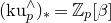 $(\mathrm{ku}_p^\wedge)_\ast = \mathbb Z_p[\beta]$
-modules:
$(\mathrm{ku}_p^\wedge)_\ast = \mathbb Z_p[\beta]$
-modules:
 \begin{align*} E_2^{0,\ast} &= \mathbb Z_p[\beta],\\ E_2^{1,\ast} &= \Sigma F_p^\wedge,\\ E_2^{2,\ast} &= \Sigma^2 T(p),\\ E_2^{r,\ast} &=0,\quad\text{if $r\neq0,1,2$}. \end{align*}
The spectral sequence degenerates at the $E_2$
-page and we have an isomorphism
$E_2$
-page and we have an isomorphism
 $$ \operatorname{THH}_\ast(\mathrm{ku})_p^\wedge = \mathbb Z_p[\beta]\oplus F_p^\wedge\oplus T(p) $$
as $\mathbb Z_p[\beta]$
-modules.
$\mathbb Z_p[\beta]$
-modules.
1.3 Outline
After a review of THH and suspension operations in §2, we prove Theorem 1.5 in §§3 and 4.
In §3, we shall set up the descent spectral sequence for $\operatorname{THH}(\mathrm{ku})\to\operatorname{THH}(\mathrm{ku}/\mathrm{MU})$
and identify the
$\operatorname{THH}(\mathrm{ku})\to\operatorname{THH}(\mathrm{ku}/\mathrm{MU})$
and identify the $E_1$
-page with a cobar complex associated with a comodule of a Hopf algebroid. More precisely, we shall use a cosimplicial resolution
$E_1$
-page with a cobar complex associated with a comodule of a Hopf algebroid. More precisely, we shall use a cosimplicial resolution
 $$ \operatorname{THH}(\mathrm{ku}) \to \lim_{\Delta} \operatorname{THH}(\mathrm{ku}/\mathrm{MU}^{\bullet + 1}) $$
using the standard Adams–Novikov resolution of $S^0\to\lim_{\Delta}\mathrm{MU}^{\bullet+1}$
as the base of the relative
$S^0\to\lim_{\Delta}\mathrm{MU}^{\bullet+1}$
as the base of the relative $\operatorname{THH}$
. In particular, we shall obtain explicit formulas for the coactions in the cobar complex using the right-unit formulas
$\operatorname{THH}$
. In particular, we shall obtain explicit formulas for the coactions in the cobar complex using the right-unit formulas $\mathrm{MU}_\ast\to\mathrm{MU}_\ast\mathrm{MU}$
.
$\mathrm{MU}_\ast\to\mathrm{MU}_\ast\mathrm{MU}$
.
Since everything will be linear over $\mathrm{ku}_\ast=\mathbb Z[\beta]$
, we shall compute the cohomology of the cobar complex modulo
$\mathrm{ku}_\ast=\mathbb Z[\beta]$
, we shall compute the cohomology of the cobar complex modulo $(p,\beta)$
and use the Bockstein spectral sequences to obtain the (p-complete) cohomology of the cobar complex, i.e. the
$(p,\beta)$
and use the Bockstein spectral sequences to obtain the (p-complete) cohomology of the cobar complex, i.e. the $E_2$
-page. The computations of Bockstein differentials are done in §4. We note that previous works [Reference Angeltveit, Hill and LawsonAHL10, Reference McClure and StaffeldtMS93, Reference AusoniAus05] also compute Bockstein spectral sequences, but the differentials are arguably easier to compute in our case because we compute the Bockstein spectral sequence of a chain complex rather than of a spectrum.
$E_2$
-page. The computations of Bockstein differentials are done in §4. We note that previous works [Reference Angeltveit, Hill and LawsonAHL10, Reference McClure and StaffeldtMS93, Reference AusoniAus05] also compute Bockstein spectral sequences, but the differentials are arguably easier to compute in our case because we compute the Bockstein spectral sequence of a chain complex rather than of a spectrum.
In §2, we put the p-completed pieces together to prove Theorem 1.4. In §6, we briefly discuss a question on $\operatorname{THH}(\mathrm{BP}\langle n\rangle)$
.
$\operatorname{THH}(\mathrm{BP}\langle n\rangle)$
.
1.4 Notation and conventions
-
– Given a nonnegative integer m and a prime number p, $\operatorname{val}_p(m)$
is the largest integer such that
$p^{\operatorname{val}_p(m)}$
divides m. We define
$\operatorname{val}_p(0)$
to be
$\infty$
.
$\operatorname{val}_p(m)$
is the largest integer such that
$p^{\operatorname{val}_p(m)}$
divides m. We define
$\operatorname{val}_p(0)$
to be
$\infty$
. -
– The word category shall always mean
$\infty$
-category. We use
$\otimes$
to denote the smash product of spectra. -
– If A is an abelian group, we shall use the same symbol A (instead of HA) to denote the Eilenberg–MacLane spectrum of A. If A is a commutative ring, then the corresponding spectrum is canonically an
$\mathbb E_\infty$
-ring spectrum.


2. Preliminaries
2.1 Topological Hochschild homology
Suppose that S is an $\mathbb E_\infty$
-ring spectrum and that R is an
$\mathbb E_\infty$
-ring spectrum and that R is an $\mathbb E_1$
-S-algebra. Then, we define the relative topological Hochschild homology as
$\mathbb E_1$
-S-algebra. Then, we define the relative topological Hochschild homology as
 $$ \operatorname{THH}(R/S) := R\otimes_{R\otimes_S R^{op}}R. $$
More generally, if M is a R-bimodule, or equivalently a $(R\otimes_S R^{op})$
-module, then the relative THH with coefficients in M is defined as
$(R\otimes_S R^{op})$
-module, then the relative THH with coefficients in M is defined as
 \begin{equation} \operatorname{THH}(R/S;M) := M\otimes_{R\otimes_SR^{op}}R. \end{equation}
In this paper, we shall only consider $\mathbb E_\infty$
-ring spectra. More precisely, we shall only consider
$\mathbb E_\infty$
-ring spectra. More precisely, we shall only consider $\operatorname{THH}(R/S;M)$
when R is an
$\operatorname{THH}(R/S;M)$
when R is an $\mathbb E_\infty$
-S-algebra and M is an
$\mathbb E_\infty$
-S-algebra and M is an $\mathbb E_\infty$
-R-algebra. In this case,
$\mathbb E_\infty$
-R-algebra. In this case, $\operatorname{THH}(R/S;M)$
naturally has a structure of an
$\operatorname{THH}(R/S;M)$
naturally has a structure of an $\mathbb E_\infty$
-R-algebra and we have an equivalence
$\mathbb E_\infty$
-R-algebra and we have an equivalence
 $$ \operatorname{THH}(R/S;M) = \operatorname{THH}(R/S)\otimes_RM $$
of $\mathbb E_\infty$
-R-algebras.
$\mathbb E_\infty$
-R-algebras.
Suppose that the following is a commutative diagram in the category of $\mathbb E_\infty$
-ring spectra.
$\mathbb E_\infty$
-ring spectra.

Then, we have an equivalence
 \begin{equation*} \operatorname{THH}(R_2\otimes_{R_1}R_3/S_2\otimes_{S_1}S_3) = \operatorname{THH}(R_2/S_2)\otimes_{\operatorname{THH}(R_1/S_1)}\operatorname{THH}(R_3/S_3). \end{equation*}
This equivalence will be used several times without reference.
2.2 Suspension elements
Suppose that S is a connective $\mathbb E_\infty$
-ring spectrum and that R is a connective
$\mathbb E_\infty$
-ring spectrum and that R is a connective $\mathbb E_\infty$
-S-algebra. Let
$\mathbb E_\infty$
-S-algebra. Let $F=\operatorname{fib}(S\to R)$
. We shall also assume that
$F=\operatorname{fib}(S\to R)$
. We shall also assume that $S_\ast\to R_\ast$
is surjective, so that
$S_\ast\to R_\ast$
is surjective, so that $F_\ast$
is an ideal of
$F_\ast$
is an ideal of $S_\ast$
.
$S_\ast$
.
Then, we define the suspension map $\sigma$
to be the composite
$\sigma$
to be the composite
 \begin{equation} \Sigma F = 0\coprod_F 0 \to R \coprod_S R \to R\otimes_S R. \end{equation}
We shall also use $\sigma$
to denote the induced map on the homotopy groups
$\sigma$
to denote the induced map on the homotopy groups $\pi_\ast(F)\to\pi_{\ast+1}(R\otimes_SR)$
.
$\pi_\ast(F)\to\pi_{\ast+1}(R\otimes_SR)$
.
Lemma 2.1. We have $\sigma(xy)=x\sigma(y)$
for any
$\sigma(xy)=x\sigma(y)$
for any $x\in S_\ast$
and
$x\in S_\ast$
and $y\in F_\ast$
. In particular,
$y\in F_\ast$
. In particular, $\sigma$
annihilates the ideal
$\sigma$
annihilates the ideal $(F_\ast)^2$
.
$(F_\ast)^2$
.
Proof. This follows from the fact that every map in Equation (2.2) is a map of S-modules.
The suspension elements will play an important role as primitive elements in Hopf algebras.
Proposition 2.2. Let R and S be as above. In addition, assume that the odd homotopy groups of S are zero and that the unit map $S_\ast\to R_\ast$
is a quotient by a regular sequence
$S_\ast\to R_\ast$
is a quotient by a regular sequence
 $$ R_\ast = S_\ast / (x_1,x_2,\dots). $$
Then, there is a $R_\ast$
-Hopf algebra structure on
$R_\ast$
-Hopf algebra structure on $\operatorname{THH}_\ast(R/S)$
such that:
$\operatorname{THH}_\ast(R/S)$
such that:
-
(a) it is free as a
$R_\ast$
-module; -
(b) the submodule of primitive elements is the free module generated by the elements
$\sigma^2 x_i$
; and -
(c) for each k and a prime p,
$(\sigma^2 x_k)^p$
is a
$R_\ast$
-linear combination of the elements
$\sigma^2 x_i$
modulo p.


Proof. Let $T=R\otimes_SR$
. The Hopf algebra structure on
$T=R\otimes_SR$
. The Hopf algebra structure on $\pi_\ast\operatorname{THH}(R/S)=\pi_\ast(R\otimes_TR)$
is given, as usual, by the map
$\pi_\ast\operatorname{THH}(R/S)=\pi_\ast(R\otimes_TR)$
is given, as usual, by the map
 $$ R\otimes_TR\xrightarrow{\operatorname{id}\otimes1\otimes\operatorname{id}} R\otimes_TR\otimes_TR = (R\otimes_TR)\otimes_R(R\otimes_TR),$$
assuming that $\pi_\ast\operatorname{THH}(R/S)$
is free over
$\pi_\ast\operatorname{THH}(R/S)$
is free over $R_\ast$
. It is a Hopf algebra rather than just a Hopf algebroid because the left and the right units
$R_\ast$
. It is a Hopf algebra rather than just a Hopf algebroid because the left and the right units $R\rightrightarrows R\otimes_TR$
are homotopic. This can be seen, for example, by observing that
$R\rightrightarrows R\otimes_TR$
are homotopic. This can be seen, for example, by observing that $\operatorname{THH}(R/S)$
is the colimit of R over the circle
$\operatorname{THH}(R/S)$
is the colimit of R over the circle $S^1$
in the category of
$S^1$
in the category of $\mathbb E_\infty$
-S-algebras and that
$\mathbb E_\infty$
-S-algebras and that $S^1$
is a connected space.
$S^1$
is a connected space.
By [Reference AngeltveitAng08, Proposition 3.6], the homotopy groups of T form a graded exterior algebra
 $$ T_\ast = \Lambda_{R_\ast}(\sigma x_1,\sigma x_2,\dots). $$
Then, the $E_2$
-page of the Künneth spectral sequence for
$E_2$
-page of the Künneth spectral sequence for $\operatorname{THH}_\ast(R/S)$
,
$\operatorname{THH}_\ast(R/S)$
,
 $$ E_2 = \operatorname{Tor}^{T_\ast}(R_\ast,R_\ast)\Rightarrow \operatorname{THH}_\ast(R/S), $$
can be computed as a divided power algebra
 $$ E_2=\Gamma_{R_\ast}[\sigma^2 x_1,\sigma^2 x_2,\dots]. $$
The spectral sequence degenerates at the $E_2$
-page since everything is concentrated in even degrees. From the
$E_2$
-page since everything is concentrated in even degrees. From the $E_2$
-page, we can see that
$E_2$
-page, we can see that $\operatorname{THH}_\ast(R/S)$
is free as a
$\operatorname{THH}_\ast(R/S)$
is free as a $R_\ast$
-module.
$R_\ast$
-module.
Taking the Whitehead tower of a spectrum defines a lax symmetric monoidal functor
 $$ \tau_{\geq\ast}:\operatorname{Sp}\to \operatorname{Fun}(\mathbb Z^{op},\operatorname{Sp}), $$
so that
 $$ \tau_{\geq\ast}R \otimes_{\tau_{\geq\ast}T}\tau_{\geq\ast}R$$
is a filtered $\mathbb E_\infty$
-ring spectrum whose underlying object is
$\mathbb E_\infty$
-ring spectrum whose underlying object is $\operatorname{THH}(R/S)$
. Taking the associated graded group, which is a symmetric monoidal process, we obtain
$\operatorname{THH}(R/S)$
. Taking the associated graded group, which is a symmetric monoidal process, we obtain
 $$ \pi_\ast R\otimes_{\pi_\ast T}\pi_\ast R, $$
whose homotopy groups are
 $$ \operatorname{Tor}^{T_\ast} (R_\ast,R_\ast).$$
This is the filtration that constructs the Künneth spectral sequence. We then see that the Künneth filtration is compatible with the coalgebra structure since the comultiplication is induced by the map
 $$ \tau_{\geq\ast}R\otimes_{\tau_{\geq\ast}T}\tau_{\geq\ast}R\xrightarrow{\operatorname{id}\otimes1\otimes\operatorname{id}}\tau_{\geq\ast}R\otimes_{\tau_{\geq\ast}T}\tau_{\geq\ast}R\otimes_{\tau_{\geq\ast}T}\tau_{\geq\ast}R$$
of filtered spectra.
It follows that the element $\sigma^2 x_k$
is primitive, since
$\sigma^2 x_k$
is primitive, since $\Delta (\sigma^2 x_k)$
must have Künneth filtration 1, and the only possibility is
$\Delta (\sigma^2 x_k)$
must have Künneth filtration 1, and the only possibility is $\sigma^2 x_k\otimes1 + 1\otimes\sigma^2 x_k$
. Conversely, any primitive element in
$\sigma^2 x_k\otimes1 + 1\otimes\sigma^2 x_k$
. Conversely, any primitive element in $\operatorname{THH}_\ast(R/S)$
must be detected by a primitive element in the associated graded group. But in the associated graded group, the primitives are linear combinations of the
$\operatorname{THH}_\ast(R/S)$
must be detected by a primitive element in the associated graded group. But in the associated graded group, the primitives are linear combinations of the $\sigma^2 x_i$
, since it is a divided power coalgebra. This proves part (b).
$\sigma^2 x_i$
, since it is a divided power coalgebra. This proves part (b).
Lastly, the (underived) quotient $(\pi_\ast(R\otimes_TR))/p$
is a
$(\pi_\ast(R\otimes_TR))/p$
is a $(R_\ast/p)$
-Hopf algebra and has a filtration such that the associated graded group is a divided power Hopf algebra on the
$(R_\ast/p)$
-Hopf algebra and has a filtration such that the associated graded group is a divided power Hopf algebra on the $\sigma^2 x_i$
. Therefore, as in the previous paragraph, the primitive elements form a free
$\sigma^2 x_i$
. Therefore, as in the previous paragraph, the primitive elements form a free $(R_\ast/p)$
-module generated by the
$(R_\ast/p)$
-module generated by the $\sigma^2 x_i$
. Then, part (c) follows since
$\sigma^2 x_i$
. Then, part (c) follows since $(\sigma^2 x_k)^p$
is primitive.
$(\sigma^2 x_k)^p$
is primitive.
Example 2.3. In this paper, we consider $\operatorname{THH}(\mathrm{ku}/\mathrm{MU})$
and
$\operatorname{THH}(\mathrm{ku}/\mathrm{MU})$
and
 $$ \mathrm{MU}\otimes_{\operatorname{THH}(\mathrm{MU})}\mathrm{MU}=\operatorname{THH}(\mathrm{MU}/\mathrm{MU}\otimes\mathrm{MU}). $$
In the notation of Definition 3.11, $\operatorname{THH}_\ast(\mathrm{MU}/\mathrm{MU}\otimes\mathrm{MU})$
is a
$\operatorname{THH}_\ast(\mathrm{MU}/\mathrm{MU}\otimes\mathrm{MU})$
is a $\mathrm{MU}_\ast$
-Hopf algebra with the primitive elements
$\mathrm{MU}_\ast$
-Hopf algebra with the primitive elements $\sigma^2 b_i$
for
$\sigma^2 b_i$
for $i\geq 1$
, and these elements will play an important role. For
$i\geq 1$
, and these elements will play an important role. For $\operatorname{THH}_\ast(\mathrm{ku}/\mathrm{MU})$
, we will need only part (c) of the previous proposition and not its Hopf algebra structure.
$\operatorname{THH}_\ast(\mathrm{ku}/\mathrm{MU})$
, we will need only part (c) of the previous proposition and not its Hopf algebra structure.
3. Descent spectral sequence
3.1 Construction of the descent spectral sequence
Definition 3.1. Let $B\to C$
be a map of
$B\to C$
be a map of $\mathbb E_\infty$
-ring spectra. Then, we can form the augmented cosimplicial diagram
$\mathbb E_\infty$
-ring spectra. Then, we can form the augmented cosimplicial diagram
 $$B \to C \rightrightarrows C \otimes_B C \mathrel{\raise6pt\hbox{$\rightarrow$}\mkern-18mu\raise-0pt\hbox{$\rightarrow$}\mkern-18mu\raise-6pt\hbox{$\rightarrow$}} \cdots$$
of $\mathbb E_\infty$
-ring spectra, called the descent diagram. If the above is a limit diagram, then we obtain the Bousfield–Kan spectral sequence
$\mathbb E_\infty$
-ring spectra, called the descent diagram. If the above is a limit diagram, then we obtain the Bousfield–Kan spectral sequence
 $$ E_1^{s,t} = \pi_t(C^{\otimes_B(s+1)})\Rightarrow \pi_{t-s}(B). $$
More generally, if M is a B-module, we have a descent diagram
 $$ M\to M\otimes_BC\rightrightarrows M\otimes_BC\otimes_BC\mathrel{\raise6pt\hbox{$\rightarrow$}\mkern-18mu\raise-0pt\hbox{$\rightarrow$}\mkern-18mu\raise-6pt\hbox{$\rightarrow$}}\cdots $$
and, if it is a limit diagram, a spectral sequence
 $$ E_1^{s,t} = \pi_t(M\otimes_B C^{\otimes_B(s+1)})\Rightarrow \pi_{t-s}(M). $$
This will be called the descent spectral sequence for $M\to M\otimes_BC$
(along
$M\to M\otimes_BC$
(along $B\to C$
). We will discuss a sufficient condition for the convergence in Lemma 3.5.
$B\to C$
). We will discuss a sufficient condition for the convergence in Lemma 3.5.
Definition 3.2. Suppose that $(k,\Gamma)$
is a graded Hopf algebroid such that
$(k,\Gamma)$
is a graded Hopf algebroid such that $\Gamma$
is flat as a k-module and A is a right
$\Gamma$
is flat as a k-module and A is a right $\Gamma$
-comodule. By the cobar complex
$\Gamma$
-comodule. By the cobar complex $\operatorname{CB}_{\Gamma}(A)$
, we mean the chain complex
$\operatorname{CB}_{\Gamma}(A)$
, we mean the chain complex
 $$ A\to A\otimes_k\Gamma\to A\otimes_k\Gamma\otimes_k\Gamma\to\cdots , $$
where the differentials are the alternating sum of comultiplication maps and the coaction maps. This is bigraded so that $\operatorname{CB}^{s,t}_{\Gamma}(A)$
is the degree-t part of
$\operatorname{CB}^{s,t}_{\Gamma}(A)$
is the degree-t part of $A\otimes_k \Gamma^{\otimes_ks}$
. The cohomology of
$A\otimes_k \Gamma^{\otimes_ks}$
. The cohomology of $\operatorname{CB}_{\Gamma}(A)$
is denoted by
$\operatorname{CB}_{\Gamma}(A)$
is denoted by $\operatorname{Ext}_{\Gamma}(A)$
, which is again bigraded. This agrees with the usual definition of
$\operatorname{Ext}_{\Gamma}(A)$
, which is again bigraded. This agrees with the usual definition of $\operatorname{Ext}$
(see, for example, [Reference RavenelRav86, A.1.2.12]).
$\operatorname{Ext}$
(see, for example, [Reference RavenelRav86, A.1.2.12]).
Proposition 3.3. In Definition 3.1, if $\pi_\ast(C\otimes_BC)$
is flat over
$\pi_\ast(C\otimes_BC)$
is flat over $\pi_\ast C$
, then
$\pi_\ast C$
, then $\pi_\ast (C\otimes_BC)$
is a Hopf algebroid over
$\pi_\ast (C\otimes_BC)$
is a Hopf algebroid over $\pi_\ast C$
,
$\pi_\ast C$
, $\pi_\ast(M\otimes_BC)$
is a comodule, and we have
$\pi_\ast(M\otimes_BC)$
is a comodule, and we have
 \begin{align*} E_1 &= \operatorname{CB}_{\pi_\ast(C\otimes_BC)}(\pi_\ast(M\otimes_BC)),\\ E_2 &= \operatorname{Ext}_{\pi_\ast(C\otimes_BC)} (\pi_\ast(M\otimes_BC)). \end{align*}
Proof. The identification of the $E_1$
-page follows from the flatness assumptions and that of the
$E_1$
-page follows from the flatness assumptions and that of the $E_2$
-page follows from the definition.
$E_2$
-page follows from the definition.
Remark 3.4. In the previous definition, if M is an $\mathbb E_\infty$
-B-algebra, then the descent spectral sequence for
$\mathbb E_\infty$
-B-algebra, then the descent spectral sequence for $M\to M\otimes_BC$
along
$M\to M\otimes_BC$
along $B\to C$
is isomorphic to the descent spectral sequence for
$B\to C$
is isomorphic to the descent spectral sequence for $M\to M\otimes_BC$
along
$M\to M\otimes_BC$
along $M\to M\otimes_BC$
. So in this case, the definition is less ambiguous without the phrase ‘along
$M\to M\otimes_BC$
. So in this case, the definition is less ambiguous without the phrase ‘along $B\to C$
’.
$B\to C$
’.
Lemma 3.5. Let $f:B\to C$
be a 1-connective map of connective
$f:B\to C$
be a 1-connective map of connective $\mathbb E_\infty$
-ring spectra. Then, for any connective B-module M, the descent spectral sequence for
$\mathbb E_\infty$
-ring spectra. Then, for any connective B-module M, the descent spectral sequence for $M\to M\otimes_BC$
converges strongly to
$M\to M\otimes_BC$
converges strongly to $\pi_\ast M$
.
$\pi_\ast M$
.
Proof. Since the descent spectral sequence is constructed from the coskeletal filtration, the lemma follows from the fact that the fiber of the map
 $$ M\to \operatorname{cosk}^s (M\otimes_B C^{\otimes_B(\bullet+1)}) $$
is $M\otimes_B I^{\otimes_B(s+1)}$
, where I is the fiber of
$M\otimes_B I^{\otimes_B(s+1)}$
, where I is the fiber of $B\to C$
(see, for example, [Reference Mathew, Naumann and NoelMNN17, Proposition 2.14]).
$B\to C$
(see, for example, [Reference Mathew, Naumann and NoelMNN17, Proposition 2.14]).
Lemma 3.6. Suppose that a map of connective $\mathbb E_\infty$
-ring spectra
$\mathbb E_\infty$
-ring spectra $f:B\to C$
induces a surjection on homotopy groups. Let
$f:B\to C$
induces a surjection on homotopy groups. Let $x\in F_\ast$
, where
$x\in F_\ast$
, where $F=\operatorname{fib}(f)$
. Then,
$F=\operatorname{fib}(f)$
. Then, $\sigma x \in \pi_\ast (C\otimes_BC)$
, considered as an element in the
$\sigma x \in \pi_\ast (C\otimes_BC)$
, considered as an element in the $E_1$
-page of the descent spectral sequence for f, is a permanent cycle and detects
$E_1$
-page of the descent spectral sequence for f, is a permanent cycle and detects $x\in B$
.
$x\in B$
.
Proof. It is enough to show that x is detected by $\sigma x$
in the equalizer
$\sigma x$
in the equalizer
 $$ \operatorname{Eq}(C\rightrightarrows C\otimes_BC). $$
This follows from chasing the diagram

from $x\in F_\ast$
.
$x\in F_\ast$
.
3.2 Complex K-theory spectrum
Until the end of §4, we shall assume that p is a fixed odd prime number and that every spectrum is p-complete. For example, we shall write $\operatorname{THH}(\mathrm{ku})$
instead of
$\operatorname{THH}(\mathrm{ku})$
instead of $\operatorname{THH}(\mathrm{ku}_p^\wedge)_p^\wedge$
.
$\operatorname{THH}(\mathrm{ku}_p^\wedge)_p^\wedge$
.
We write ku for the connective cover of the complex K-theory spectrum KU equipped with the standard complex orientation $\mathrm{MU}\to\mathrm{ku}$
, which can be lifted to be an
$\mathrm{MU}\to\mathrm{ku}$
, which can be lifted to be an $\mathbb E_\infty$
orientation according to [Reference JoachimJoa04].
$\mathbb E_\infty$
orientation according to [Reference JoachimJoa04].
We shall compute the descent spectral sequence for
 $$ \operatorname{THH}(\mathrm{ku})\to\operatorname{THH}(\mathrm{ku}/\mathrm{MU})=\operatorname{THH}(\mathrm{ku})\otimes_{\operatorname{THH}(\mathrm{MU})}\mathrm{MU} $$
along $\operatorname{THH}(\mathrm{MU})\to \mathrm{MU}$
. More generally, for
$\operatorname{THH}(\mathrm{MU})\to \mathrm{MU}$
. More generally, for $M=\mathbb F_p$
or
$M=\mathbb F_p$
or $\mathbb Z_p$
with a canonical ku-algebra structure, we shall compute the descent spectral sequence for
$\mathbb Z_p$
with a canonical ku-algebra structure, we shall compute the descent spectral sequence for
 $$ \operatorname{THH}(\mathrm{ku};M)\to\operatorname{THH}(\mathrm{ku}/\mathrm{MU};M). $$
Let $E_r^{\ast,\ast}(\operatorname{THH}(\mathrm{ku};M))$
denote the
$E_r^{\ast,\ast}(\operatorname{THH}(\mathrm{ku};M))$
denote the $E_r$
-page of this descent spectral sequence. Until the end of §4, let us write
$E_r$
-page of this descent spectral sequence. Until the end of §4, let us write
 \begin{align*} \Gamma &:= \mathrm{MU}\otimes_{\operatorname{THH}(\mathrm{MU})}\mathrm{MU}=\operatorname{THH}(\mathrm{MU}/\mathrm{MU}\otimes\mathrm{MU}),\\ A&:= \operatorname{THH}(\mathrm{ku}/\mathrm{MU}). \end{align*}
Using Propositions 2.2 and 3.3, we note a few things about the homotopy groups of these ring spectra.
-
– Both
$A_\ast$
and
$\Gamma_\ast$
are commutative even-graded rings. -
– We find that
$\Gamma_\ast$
is a
$\mathrm{MU}_\ast$
-Hopf algebra and
$A_\ast$
is a right
$\Gamma_\ast$
-comodule algebra. We shall write
$\eta_R:A_\ast\to A_\ast\otimes\Gamma_\ast$
for the coaction map, for reasons to be explained in Proposition 3.10. -
– We can identify
$E_1^{\ast,\ast}(\operatorname{THH}(\mathrm{ku}))$
with the cobar complex where we write
$$ \operatorname{CB}_{\Gamma_\ast}(A_\ast)= (A_\ast\xrightarrow{D^0} A_\ast\otimes_{\mathrm{MU}_\ast}\Gamma_\ast\xrightarrow{D^1} A_\ast\otimes_{\mathrm{MU}_\ast}\Gamma_\ast\otimes_{\mathrm{MU}_\ast}\Gamma_\ast\xrightarrow{D^2}\cdots),$$
$D^0, D^1, \dots$
for the differentials in
$\operatorname{CB}_{\Gamma_\ast}(A_\ast)$
. These are the
$d_1$
differentials in the descent spectral sequence.






Remark 3.7. Suppose that $B\to C$
is a map of
$B\to C$
is a map of $\mathbb E_\infty$
-ring spectra. Instead of the coskeletal filtration of the descent diagram for
$\mathbb E_\infty$
-ring spectra. Instead of the coskeletal filtration of the descent diagram for $B\to C$
, there is an alternative filtration using Whitehead covers. The kth filtration of B is given by
$B\to C$
, there is an alternative filtration using Whitehead covers. The kth filtration of B is given by
 $$ \operatorname{Tot}(\tau_{\geq 2k} C^{\otimes_B (\bullet+1)}).$$
If we further assume that $C^{\otimes_B(s+1)}$
has no odd homotopy groups for all
$C^{\otimes_B(s+1)}$
has no odd homotopy groups for all $s\geq0$
, then this filtration gives us a shearing of the descent spectral sequence in the sense that we have
$s\geq0$
, then this filtration gives us a shearing of the descent spectral sequence in the sense that we have
 $$ ^\backprime E_r^{k,3k-s} = E_{2r+1}^{s,2k}, $$
where the left-hand side is the spectral sequence associated with the new filtration and the right-hand side is the descent spectral sequence. More precisely, they are related by the décalage [Reference AntieauAnt24] and by doubling the speed of the filtration.
In our case of $B=\operatorname{THH}(\mathrm{ku})$
and
$B=\operatorname{THH}(\mathrm{ku})$
and $C=\operatorname{THH}(\mathrm{ku}/\mathrm{MU})$
, the new filtration using Whitehead covers is an example of the even/motivic filtration of Hahn, Raksit, and Wilson [Reference Hahn, Raksit and WilsonHRW25, Definition 4.1.2], since C is evenly free over B in their sense.
$C=\operatorname{THH}(\mathrm{ku}/\mathrm{MU})$
, the new filtration using Whitehead covers is an example of the even/motivic filtration of Hahn, Raksit, and Wilson [Reference Hahn, Raksit and WilsonHRW25, Definition 4.1.2], since C is evenly free over B in their sense.
Lemma 3.8. $\operatorname{CB}_{\Gamma_\ast}(A_\ast)$
is a chain complex of free
$\operatorname{CB}_{\Gamma_\ast}(A_\ast)$
is a chain complex of free $\mathrm{ku}_\ast$
-modules. Therefore, we have identifications
$\mathrm{ku}_\ast$
-modules. Therefore, we have identifications
 \begin{align*} E_1(\operatorname{THH}(\mathrm{ku};\mathbb Z_p)) &= \operatorname{CB}_{\Gamma_\ast}(A_\ast/\beta),\\ E_2(\operatorname{THH}(\mathrm{ku};\mathbb Z_p)) &= \operatorname{Ext}_{\Gamma_\ast}(A_\ast/\beta),\\ E_1(\operatorname{THH}(\mathrm{ku};\mathbb F_p)) &= \operatorname{CB}_{\Gamma_\ast}(A_\ast/(p,\beta)),\\ E_2(\operatorname{THH}(\mathrm{ku};\mathbb F_p)) &= \operatorname{Ext}_{\Gamma_\ast}(A_\ast/(p,\beta)). \end{align*}
Proof. From Example 2.3, $A_\ast$
is free as a
$A_\ast$
is free as a $\mathrm{ku}_\ast$
-module and
$\mathrm{ku}_\ast$
-module and $\Gamma_\ast$
is free as a
$\Gamma_\ast$
is free as a $\mathrm{MU}_\ast$
-module.
$\mathrm{MU}_\ast$
-module.
Notation 3.9. From this point, all ordinary modules or ordinary rings will naturally be modules or algebras over $\mathrm{MU}_\ast$
, and all tensor product
$\mathrm{MU}_\ast$
, and all tensor product $\otimes$
will be over
$\otimes$
will be over $\mathrm{MU}_\ast$
unless the base ring is explicitly written. We shall continue to write the base for the tensor product of spectra unless it is over the sphere spectrum.
$\mathrm{MU}_\ast$
unless the base ring is explicitly written. We shall continue to write the base for the tensor product of spectra unless it is over the sphere spectrum.
There is an alternative description of the descent spectral sequence. The augmented cosimplicial diagram
 $$ S^0 \to \mathrm{MU}\rightrightarrows \mathrm{MU}^{\otimes2} \mathrel{\raise6pt\hbox{$\rightarrow$}\mkern-18mu\raise-0pt\hbox{$\rightarrow$}\mkern-18mu\raise-6pt\hbox{$\rightarrow$}} \cdots$$
induces an augmented cosimplicial diagram
 \begin{equation} \operatorname{THH}(\mathrm{ku})\to\operatorname{THH}(\mathrm{ku}/\mathrm{MU})\rightrightarrows \operatorname{THH}(\mathrm{ku}/\mathrm{MU}^{\otimes2}) \mathrel{\raise6pt\hbox{$\rightarrow$}\mkern-18mu\raise-0pt\hbox{$\rightarrow$}\mkern-18mu\raise-6pt\hbox{$\rightarrow$}} \cdots \end{equation}
of $\mathbb E_\infty$
-ring spectra. The following proposition is immediate from the definitions.
$\mathbb E_\infty$
-ring spectra. The following proposition is immediate from the definitions.
Proposition 3.10. The augmented cosimplicial diagram (3.1) is equivalent to the descent diagram for $\operatorname{THH}(\mathrm{ku})\to\operatorname{THH}(\mathrm{ku}/\mathrm{MU})$
. Furthermore, under the identification
$\operatorname{THH}(\mathrm{ku})\to\operatorname{THH}(\mathrm{ku}/\mathrm{MU})$
. Furthermore, under the identification $\operatorname{THH}_\ast(\mathrm{ku}/\mathrm{MU}^{\otimes2})=A_\ast\otimes\Gamma_\ast$
, the two maps
$\operatorname{THH}_\ast(\mathrm{ku}/\mathrm{MU}^{\otimes2})=A_\ast\otimes\Gamma_\ast$
, the two maps
 $$ \eta_L,\eta_R:\operatorname{THH}_\ast(\mathrm{ku}/\mathrm{MU})\to\operatorname{THH}_\ast(\mathrm{ku}/\mathrm{MU}^{\otimes2})$$
induced by the left and right units $\eta_L,\eta_R:\mathrm{MU}\to \mathrm{MU}^{\otimes2}$
can be identified with
$\eta_L,\eta_R:\mathrm{MU}\to \mathrm{MU}^{\otimes2}$
can be identified with $\operatorname{id}\otimes1$
and the coaction map
$\operatorname{id}\otimes1$
and the coaction map $A_\ast\to A_\ast\otimes\Gamma_\ast$
, respectively.
$A_\ast\to A_\ast\otimes\Gamma_\ast$
, respectively.
Definition 3.11. Following the classical notation, we write $x_1,x_2,\dots$
with
$x_1,x_2,\dots$
with $|x_i|=2i$
for the polynomial generators of the Lazard ring
$|x_i|=2i$
for the polynomial generators of the Lazard ring $\mathrm{MU}_\ast$
, and we write
$\mathrm{MU}_\ast$
, and we write $b_1,b_2,\dots$
for the generators of
$b_1,b_2,\dots$
for the generators of $\mathrm{MU}_\ast\mathrm{MU} = \mathrm{MU}_\ast[b_1,b_2,\dots]$
as a
$\mathrm{MU}_\ast\mathrm{MU} = \mathrm{MU}_\ast[b_1,b_2,\dots]$
as a $\mathrm{MU}_\ast$
-algebra, where
$\mathrm{MU}_\ast$
-algebra, where $\mathrm{MU}_\ast\mathrm{MU}$
is given the algebra structure by the left unit
$\mathrm{MU}_\ast\mathrm{MU}$
is given the algebra structure by the left unit $\mathrm{MU}_\ast\to\mathrm{MU}_\ast\mathrm{MU}$
and the
$\mathrm{MU}_\ast\to\mathrm{MU}_\ast\mathrm{MU}$
and the $b_i$
vanish under the multiplication map
$b_i$
vanish under the multiplication map $\mathrm{MU}_\ast\mathrm{MU}\to\mathrm{MU}_\ast$
. There are many choices for the generators, and for now, we only require that
$\mathrm{MU}_\ast\mathrm{MU}\to\mathrm{MU}_\ast$
. There are many choices for the generators, and for now, we only require that $x_1$
maps to
$x_1$
maps to $\beta$
under
$\beta$
under
 $$ \mathrm{MU}_\ast\to \mathrm{ku}_\ast=\mathbb Z_p[\beta] $$
and that $x_i$
maps to zero for
$x_i$
maps to zero for $i\geq 2$
. We shall give more specific choices of generators in Lemma 3.16.
$i\geq 2$
. We shall give more specific choices of generators in Lemma 3.16.
For the lightness of notation, we shall often write $v_k$
instead of
$v_k$
instead of $x_{p^k-1}$
when
$x_{p^k-1}$
when $k\geq 2$
and
$k\geq 2$
and $t_k$
instead of
$t_k$
instead of $b_{p^k-1}$
when
$b_{p^k-1}$
when $k\geq 1$
. Note that we do not write
$k\geq 1$
. Note that we do not write $v_1$
for
$v_1$
for $x_{p-1}$
, because
$x_{p-1}$
, because $x_{p-1}$
maps to 0 in
$x_{p-1}$
maps to 0 in $\mathrm{ku}_\ast$
, while it is more natural that a class named
$\mathrm{ku}_\ast$
, while it is more natural that a class named $v_1$
maps to a nonzero class in
$v_1$
maps to a nonzero class in $\mathrm{ku}_\ast$
.
$\mathrm{ku}_\ast$
.
Notation 3.12. The elements $x_i\in\mathrm{MU}_\ast$
for
$x_i\in\mathrm{MU}_\ast$
for $i\geq 2$
and
$i\geq 2$
and $b_i\in\mathrm{MU}_\ast\mathrm{MU}$
for
$b_i\in\mathrm{MU}_\ast\mathrm{MU}$
for $i\geq 1$
admit double suspensions
$i\geq 1$
admit double suspensions $\sigma^2 x_i\in A_\ast$
and
$\sigma^2 x_i\in A_\ast$
and $\sigma^2 b_i\in \Gamma_\ast$
. In the cobar complex
$\sigma^2 b_i\in \Gamma_\ast$
. In the cobar complex $\operatorname{CB}_{\Gamma_\ast}(A_\ast)$
, we shall write
$\operatorname{CB}_{\Gamma_\ast}(A_\ast)$
, we shall write $\sigma^2 x_i$
(or
$\sigma^2 x_i$
(or $\sigma^2 v_i$
) for the corresponding element in either
$\sigma^2 v_i$
) for the corresponding element in either $A_\ast$
or
$A_\ast$
or $A_\ast\otimes\Gamma_\ast$
. Which element the notation is referring to will be clear from the context. Similarly, we shall write
$A_\ast\otimes\Gamma_\ast$
. Which element the notation is referring to will be clear from the context. Similarly, we shall write $\sigma^2 b_i$
(or
$\sigma^2 b_i$
(or $\sigma^2 t_i$
) for the corresponding element in
$\sigma^2 t_i$
) for the corresponding element in $A_\ast\otimes\Gamma_\ast$
. We will not need any notation for elements in
$A_\ast\otimes\Gamma_\ast$
. We will not need any notation for elements in $A_\ast\otimes\Gamma_\ast^{\otimes s}$
for
$A_\ast\otimes\Gamma_\ast^{\otimes s}$
for $s\geq 2$
.
$s\geq 2$
.
The following two remarks hold for any choice of generators.
Remark 3.13. Consider the descent spectral sequence for $\operatorname{THH}(\mathrm{MU})\to\operatorname{THH}(\mathrm{MU}/\mathrm{MU})$
, whose
$\operatorname{THH}(\mathrm{MU})\to\operatorname{THH}(\mathrm{MU}/\mathrm{MU})$
, whose $E_1$
-page is
$E_1$
-page is $\operatorname{CB}_{\Gamma_\ast}(\mathrm{MU}_\ast)$
. Since
$\operatorname{CB}_{\Gamma_\ast}(\mathrm{MU}_\ast)$
. Since
 $$ \operatorname{THH}_\ast(\mathrm{MU}) = \Lambda_{\mathrm{MU}_\ast}(\sigma b_1,\sigma b_2,\dots),$$
we can see, by Lemma 3.6, that the element $\sigma^2 b_i\in \operatorname{CB}_{\Gamma_\ast}^1(\mathrm{MU}_\ast)$
is a permanent cycle in the descent spectral sequence for any i and that it detects
$\sigma^2 b_i\in \operatorname{CB}_{\Gamma_\ast}^1(\mathrm{MU}_\ast)$
is a permanent cycle in the descent spectral sequence for any i and that it detects $\sigma b_i\in\operatorname{THH}_\ast(\mathrm{MU})$
.
$\sigma b_i\in\operatorname{THH}_\ast(\mathrm{MU})$
.
Mapping to the descent spectral sequence for $\operatorname{THH}(\mathrm{ku})\to\operatorname{THH}(\mathrm{ku}/\mathrm{MU})$
, we can see that
$\operatorname{THH}(\mathrm{ku})\to\operatorname{THH}(\mathrm{ku}/\mathrm{MU})$
, we can see that $\sigma^2 b_i\in \operatorname{CB}^1_{\Gamma_\ast}(A_\ast)$
is a permanent cycle in this descent spectral sequence and detects
$\sigma^2 b_i\in \operatorname{CB}^1_{\Gamma_\ast}(A_\ast)$
is a permanent cycle in this descent spectral sequence and detects $\sigma b_i\in\operatorname{THH}_\ast(\mathrm{ku})$
. Here,
$\sigma b_i\in\operatorname{THH}_\ast(\mathrm{ku})$
. Here, $\sigma b_i$
is the suspension of the class
$\sigma b_i$
is the suspension of the class $b_i\in\mathrm{ku}_\ast\mathrm{ku}$
, which is defined to be the image of
$b_i\in\mathrm{ku}_\ast\mathrm{ku}$
, which is defined to be the image of $b_i\in\mathrm{MU}_\ast\mathrm{MU}$
.
$b_i\in\mathrm{MU}_\ast\mathrm{MU}$
.
Remark 3.14. There is a multiplicative structure on the descent spectral sequence, which is represented in $E_1=\operatorname{CB}_{\Gamma_\ast}(A_\ast)$
by the standard formula for the cup product of cocycles. We shall only be interested in the multiplication by
$E_1=\operatorname{CB}_{\Gamma_\ast}(A_\ast)$
by the standard formula for the cup product of cocycles. We shall only be interested in the multiplication by $\sigma^2 b_i\in A_\ast\otimes\Gamma_\ast$
, which is a permanent cycle by the previous remark. In this case, we can check that the cup-product formula in the
$\sigma^2 b_i\in A_\ast\otimes\Gamma_\ast$
, which is a permanent cycle by the previous remark. In this case, we can check that the cup-product formula in the $E_1$
-page for
$E_1$
-page for $x\in A_\ast\otimes\Gamma_\ast^{\otimes s}$
and
$x\in A_\ast\otimes\Gamma_\ast^{\otimes s}$
and $\sigma^2 b_i$
equals
$\sigma^2 b_i$
equals $x\otimes\sigma^2 b_i\in A_\ast\otimes\Gamma_\ast^{\otimes (s+1)}$
.
$x\otimes\sigma^2 b_i\in A_\ast\otimes\Gamma_\ast^{\otimes (s+1)}$
.
Lemma 3.15. For any choice of generators in Definition 3.11, we have
 $$ (\sigma^2 v_k)^p \equiv \sigma^2 v_{k+1} \pmod{p,\beta} $$
for $k\geq 2$
and
$k\geq 2$
and
 $$ (\sigma^2 x_{p-1})^p \equiv\sigma^2 v_2 \pmod{p,\beta}$$
in $A_\ast$
up to a p-adic unit. Similarly, we have
$A_\ast$
up to a p-adic unit. Similarly, we have
 $$ (\sigma^2 b_i)^p \equiv \sigma^2 b_{pi+p-1} \pmod{p,x_1,x_2,\ldots} $$
for $i\geq 1$
in
$i\geq 1$
in $\Gamma_\ast$
up to a p-adic unit.
$\Gamma_\ast$
up to a p-adic unit.
Proof. For $A_\ast$
, the proof is the same as the proof of [Reference Hahn and WilsonHW22, Proposition 2.5.3]. For
$A_\ast$
, the proof is the same as the proof of [Reference Hahn and WilsonHW22, Proposition 2.5.3]. For $\Gamma_\ast$
, it is similar and we shall sketch the proof. We wish to show that
$\Gamma_\ast$
, it is similar and we shall sketch the proof. We wish to show that $(\sigma^2 v_k)^p=\sigma^2 v_{k+1}$
in
$(\sigma^2 v_k)^p=\sigma^2 v_{k+1}$
in
 $$ \Gamma_\ast \otimes_{\mathrm{MU}_\ast} \mathbb F_p = \pi_\ast (\Gamma\otimes_\mathrm{MU}\mathbb F_p). $$
Since base changing along $\mathrm{MU}\to\mathbb F_p$
is a symmetric monoidal functor, we have
$\mathrm{MU}\to\mathbb F_p$
is a symmetric monoidal functor, we have
 $$ \Gamma\otimes_{\mathrm{MU}}\mathbb F_p = \mathbb F_p\otimes_{\operatorname{THH}(\mathrm{MU};\mathbb F_p)}\mathbb F_p , $$
where $\operatorname{THH}(\mathrm{MU};\mathbb F_p) = \mathbb F_p\otimes_{\mathbb F_p\otimes\mathrm{MU}}\mathbb F_p$
, again by base change. By the stability of Dyer–Lashof operations, we have
$\operatorname{THH}(\mathrm{MU};\mathbb F_p) = \mathbb F_p\otimes_{\mathbb F_p\otimes\mathrm{MU}}\mathbb F_p$
, again by base change. By the stability of Dyer–Lashof operations, we have
 $$ (\sigma^2 b_i)^p = Q_0(\sigma^2 b_i) = \sigma^2 (Q_2 b_i).$$
Then, the statement follows from the computation of the operation $Q_2$
in
$Q_2$
in $(\mathbb F_p)_{\ast}\mathrm{MU}=H_\ast(BU;\mathbb F_p)$
, done in [Reference KochmanKoc71, Theorem 6].
$(\mathbb F_p)_{\ast}\mathrm{MU}=H_\ast(BU;\mathbb F_p)$
, done in [Reference KochmanKoc71, Theorem 6].
Lemma 3.16. We can choose the generators $x_2,x_3,\dots,b_1,b_2,\dots$
so that the following properties hold.
$x_2,x_3,\dots,b_1,b_2,\dots$
so that the following properties hold.
-
(a) There is a sequence of p-adic units
$\delta_0=1, \delta_1,\delta_2,\dots\in\mathbb Z_p^\times$
such that
$(\sigma^2 v_2)^{p^k}\equiv\delta_k\sigma^2 v_{k+2}\pmod p$
for
$k\geq 0$
in
$A_\ast$
. -
(b) We have
$(\sigma^2 t_1)^{p^k}\equiv\delta_k\sigma^2 t_{k+1}\pmod p$
for
$k\geq0$
in
$\Gamma_\ast$
with the same sequence
$\delta_1,\delta_2,\dots$
as in property (a). -
(c) We have
$(\sigma^2 b_1)^p \equiv \sigma^2 b_{2p-1} \pmod p$
in
$\Gamma_\ast$
. -
(d) The coaction of the element
$\sigma^2 v_k\in A_\ast$
is given as and the coaction of the element
$$ \eta_R \sigma^2 v_k = \sigma^2 v_k + p\sigma^2 t_k + \beta^{p^k-p^{k-1}}\sigma^2 t_{k-1} $$
$\sigma^2 x_{p-1}$
is given as
$$ \eta_R \sigma^2 x_{p-1} = \sigma^2 x_{p-1}+p\sigma^2 t_1 + \beta^{p-2}\sigma^2 b_1. $$
-
(e) There is a constant
$\delta'$
such that the coaction of the element
$\sigma^2 x_{2p-1}$
is given as
$$ \eta_R\sigma^2 x_{2p-1} = \sigma^2 x_{2p-1} + \sigma^2 b_{2p-1} + \delta' \beta^p\sigma^2 t_1. $$
-
(f) The constant
$\delta'$
in property (e) is a p-adic unit.










Proof. We first note that we do not need to require that the sequences $\delta_1,\delta_2,\dots$
of p-adic units appearing in properties (a) and (b) are the same sequences, because it follows automatically from the first equation of property (d) by taking the pth powers mod p and the fact that the statement only depends on the mod p reductions of the
$\delta_1,\delta_2,\dots$
of p-adic units appearing in properties (a) and (b) are the same sequences, because it follows automatically from the first equation of property (d) by taking the pth powers mod p and the fact that the statement only depends on the mod p reductions of the $\delta_i$
.
$\delta_i$
.
By the naturality of $\sigma$
, we have
$\sigma$
, we have $\eta_R(\sigma^2 \alpha) = \sigma^2 \eta_R(\alpha)$
for any
$\eta_R(\sigma^2 \alpha) = \sigma^2 \eta_R(\alpha)$
for any $\alpha\in \pi_\ast\operatorname{fib}(\mathrm{MU}\to\mathrm{ku})$
. Therefore, the lemma will be proved using properties of the right unit
$\alpha\in \pi_\ast\operatorname{fib}(\mathrm{MU}\to\mathrm{ku})$
. Therefore, the lemma will be proved using properties of the right unit $\mathrm{MU}_\ast\to\mathrm{MU}_\ast\mathrm{MU}$
.
$\mathrm{MU}_\ast\to\mathrm{MU}_\ast\mathrm{MU}$
.
Setup. Let us outline our strategy. Starting from some set of polynomial generators for $\mathrm{MU}_\ast$
and
$\mathrm{MU}_\ast$
and $\mathrm{MU}_\ast\mathrm{MU}$
as in Definition 3.11, we shall try to modify the generators so that they satisfy the lemma.
$\mathrm{MU}_\ast\mathrm{MU}$
as in Definition 3.11, we shall try to modify the generators so that they satisfy the lemma.
Let us write $I_0=(x_2,x_3,\dots)\subseteq \mathrm{MU}_\ast$
and
$I_0=(x_2,x_3,\dots)\subseteq \mathrm{MU}_\ast$
and $I_1=(x_2,x_3,\dots,b_1,b_2,\dots)\subseteq \mathrm{MU}_\ast\mathrm{MU}$
for the kernel ideals of maps to
$I_1=(x_2,x_3,\dots,b_1,b_2,\dots)\subseteq \mathrm{MU}_\ast\mathrm{MU}$
for the kernel ideals of maps to $\mathrm{ku}_\ast$
. Being kernels of maps to
$\mathrm{ku}_\ast$
. Being kernels of maps to $\mathrm{ku}_\ast$
implies that
$\mathrm{ku}_\ast$
implies that $\eta_L$
and
$\eta_L$
and $\eta_R$
map
$\eta_R$
map $I_0$
to
$I_0$
to $I_1$
. In addition, by Lemma 2.1,
$I_1$
. In addition, by Lemma 2.1, $\sigma^2$
annihilates
$\sigma^2$
annihilates $I_0^2$
and
$I_0^2$
and $I_1^2$
. In other words, there is the following commutative diagram for
$I_1^2$
. In other words, there is the following commutative diagram for $?=L,R$
, where
$?=L,R$
, where $\overline{\eta_?}$
denotes the top arrow.
$\overline{\eta_?}$
denotes the top arrow.

The quotients $I_0/I_0^2$
and
$I_0/I_0^2$
and $I_1/I_1^2$
are naturally modules over
$I_1/I_1^2$
are naturally modules over $\mathrm{MU}_\ast/I_0=\mathrm{MU}_\ast\mathrm{MU}/I_1=\mathrm{ku}_\ast$
. As a
$\mathrm{MU}_\ast/I_0=\mathrm{MU}_\ast\mathrm{MU}/I_1=\mathrm{ku}_\ast$
. As a $\mathrm{ku}_\ast$
-module,
$\mathrm{ku}_\ast$
-module, $I_0/I_0^2$
is a free graded module generated by
$I_0/I_0^2$
is a free graded module generated by $\{\overline{x_2},\overline{x_3},\dots\}$
, where
$\{\overline{x_2},\overline{x_3},\dots\}$
, where $\overline{x_i}$
is the image of
$\overline{x_i}$
is the image of $x_i\in I_0$
. Similarly,
$x_i\in I_0$
. Similarly, $I_1/I_1^2$
is free and there is a natural splitting
$I_1/I_1^2$
is free and there is a natural splitting
 $$ I_1/I_1^2=\overline{\eta_L}(I_0/I_0^2) \oplus \mathrm{ku}_\ast\{\overline{b_1},\overline{b_2},\dots\} $$
induced by the multiplication map $\mathrm{MU}_\ast\mathrm{MU}\to\mathrm{MU}$
.
$\mathrm{MU}_\ast\mathrm{MU}\to\mathrm{MU}$
.
We also observe that $\overline{\eta_L}$
and
$\overline{\eta_L}$
and $\overline{\eta_R}$
are
$\overline{\eta_R}$
are $\mathrm{ku}_\ast$
-linear. For
$\mathrm{ku}_\ast$
-linear. For $\overline{\eta_L}$
, this is clear since
$\overline{\eta_L}$
, this is clear since $\eta_L(x_1)=x_1$
. For
$\eta_L(x_1)=x_1$
. For $\overline{\eta_R}$
, this can be seen by either observing that the vertical arrows in the above square are injective or by a direct computation:
$\overline{\eta_R}$
, this can be seen by either observing that the vertical arrows in the above square are injective or by a direct computation:
 $$ \eta_R(x_1\alpha)-x_1\eta_R(\alpha)=b_1\eta_R(\alpha)\in I_1^2\qquad\forall\alpha\in I_0.$$
For the purpose of proving this lemma, we only need to choose a set of generators of $I_0/I_0^2$
and
$I_0/I_0^2$
and $I_1/I_1^2$
as free
$I_1/I_1^2$
as free $\mathrm{ku}_\ast$
-modules. Any set of generators lift to a set of polynomial generators for
$\mathrm{ku}_\ast$
-modules. Any set of generators lift to a set of polynomial generators for $\mathrm{MU}_\ast$
and
$\mathrm{MU}_\ast$
and $\mathrm{MU}_\ast\mathrm{MU}$
, and the choice of a lift is irrelevant, since
$\mathrm{MU}_\ast\mathrm{MU}$
, and the choice of a lift is irrelevant, since $\sigma^2$
annihilates any difference.
$\sigma^2$
annihilates any difference.
The reduction argument. For any $k\geq 2$
, we have
$k\geq 2$
, we have
 \begin{equation} \overline{\eta_R}(\overline{x_k}) = \overline{x_k} +\sum_{i=1}^k c_{k,i} \beta^{k-i}\overline{b_i},\end{equation}
for some $c_{k,0},\dots,c_{k,k}\in\mathbb Z_p$
. It is a standard fact [Reference RavenelRav86, Theorem 3.1.5] that the top coefficient
$c_{k,0},\dots,c_{k,k}\in\mathbb Z_p$
. It is a standard fact [Reference RavenelRav86, Theorem 3.1.5] that the top coefficient $c_{k,k}$
is a p-adic unit unless
$c_{k,k}$
is a p-adic unit unless $k+1$
is a power of p and that we have
$k+1$
is a power of p and that we have $c_{k,k}\in p\mathbb Z_p^\times$
if
$c_{k,k}\in p\mathbb Z_p^\times$
if $k+1$
is a power of p. Note that by counitality of the Hopf algebroid
$k+1$
is a power of p. Note that by counitality of the Hopf algebroid $\mathrm{MU}_\ast\mathrm{MU}$
, there are no terms of the form
$\mathrm{MU}_\ast\mathrm{MU}$
, there are no terms of the form $\beta^{k-i}\overline{x_i}$
on the right-hand side.
$\beta^{k-i}\overline{x_i}$
on the right-hand side.
Let us consider $(c_{k,i})$
as a matrix, indexed by
$(c_{k,i})$
as a matrix, indexed by $\{2,3,\dots\}\times\{1,2,\dots\}$
, i.e. it is an infinite square matrix with the first row missing. Then, it is ‘lower-triangular’ in the sense that
$\{2,3,\dots\}\times\{1,2,\dots\}$
, i.e. it is an infinite square matrix with the first row missing. Then, it is ‘lower-triangular’ in the sense that $c_{k,i}=0$
for
$c_{k,i}=0$
for $i \gt k$
, and the ‘diagonal’ entries
$i \gt k$
, and the ‘diagonal’ entries $c_{k,k}$
are units except for those such that
$c_{k,k}$
are units except for those such that $k+1$
is a power of p.
$k+1$
is a power of p.
Since $\overline{\eta_R}$
is
$\overline{\eta_R}$
is $\mathrm{ku}_\ast$
-linear, modifying a generator of
$\mathrm{ku}_\ast$
-linear, modifying a generator of $I_0/I_0^2$
, by adding multiples of
$I_0/I_0^2$
, by adding multiples of $\beta^{k-j}x_j$
to
$\beta^{k-j}x_j$
to $x_k$
for example, has an effect of adding the same multiple of the jth row to the kth row. As the diagonal entries are mostly units, we can perform the row operations to make the matrix diagonal except on the columns with a non-unit diagonal entry and the first column. More precisely, suppose that we have
$x_k$
for example, has an effect of adding the same multiple of the jth row to the kth row. As the diagonal entries are mostly units, we can perform the row operations to make the matrix diagonal except on the columns with a non-unit diagonal entry and the first column. More precisely, suppose that we have
 $$ \overline{\eta_R}(\overline{x_k})=\overline{x_k}+\sum_{i=1}^k c_{k,i}\beta^{k-i}\overline{b_i}.$$
Then, we take the greatest index $i_0\in \{2,\dots,k-1\}\backslash\{p^j-1:j\geq1\}$
such that
$i_0\in \{2,\dots,k-1\}\backslash\{p^j-1:j\geq1\}$
such that $c_{k,i_0}\neq 0$
, if one exists. Then, if we replace
$c_{k,i_0}\neq 0$
, if one exists. Then, if we replace $\overline{x_k}$
by
$\overline{x_k}$
by $\overline{x_k}-c_{i_0,i_0}^{-1}c_{k,i_0}\beta^{k-i_0}\overline{x_{i_0}}$
, we effectively make
$\overline{x_k}-c_{i_0,i_0}^{-1}c_{k,i_0}\beta^{k-i_0}\overline{x_{i_0}}$
, we effectively make $c_{k,i_0}=0$
. Repeating this, we arrive at a generator
$c_{k,i_0}=0$
. Repeating this, we arrive at a generator $\overline{x_k}$
such that
$\overline{x_k}$
such that
 $$ \overline{\eta_R}(\overline{x_k}) = \overline{x_k} +c_{k,k}\overline{b_k} +\bigg(\sum_{p^j-1<k}c_{k,p^j-1}\beta^{k-p^j+1}\overline{t_j}\bigg) + c_{k,1}\beta^{k-1}\overline{b_1}. $$
This reduction argument will be used multiple times in the following proof.
Step 1: choosing $x_{p-1},t_1,$
and
$x_{p-1},t_1,$
and $b_1$
to satisfy property (d). Let
$b_1$
to satisfy property (d). Let $i_Q:(\mathrm{BP}_\ast,\mathrm{BP}_\ast\mathrm{BP})\to(\mathrm{MU}_\ast,\mathrm{MU}_\ast\mathrm{MU})$
be the map of Hopf algebroids induced by the Quillen idempotent and let
$i_Q:(\mathrm{BP}_\ast,\mathrm{BP}_\ast\mathrm{BP})\to(\mathrm{MU}_\ast,\mathrm{MU}_\ast\mathrm{MU})$
be the map of Hopf algebroids induced by the Quillen idempotent and let $v_1',v_2',\dots,t_1',t_2',\ldots$
be the Hazewinkel generators [Reference RavenelRav86, A2.2] for
$v_1',v_2',\dots,t_1',t_2',\ldots$
be the Hazewinkel generators [Reference RavenelRav86, A2.2] for $\mathrm{BP}_\ast=\mathbb Z_p[v_1',\dots]$
and
$\mathrm{BP}_\ast=\mathbb Z_p[v_1',\dots]$
and $\mathrm{BP}_\ast\mathrm{BP}=\mathrm{BP}_\ast[t_1',\dots]$
. Note that
$\mathrm{BP}_\ast\mathrm{BP}=\mathrm{BP}_\ast[t_1',\dots]$
. Note that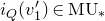 $i_Q(v_1')\in\mathrm{MU}_\ast$
is the coefficient of
$i_Q(v_1')\in\mathrm{MU}_\ast$
is the coefficient of $X^p$
in the p-series of the universal formal group law mod p. This means that the image of
$X^p$
in the p-series of the universal formal group law mod p. This means that the image of $i_Q(v_1')$
in
$i_Q(v_1')$
in $\mathrm{ku}_\ast$
is
$\mathrm{ku}_\ast$
is $\varepsilon\beta^{p-1}$
for some p-adic unit
$\varepsilon\beta^{p-1}$
for some p-adic unit $\varepsilon$
. We define
$\varepsilon$
. We define $x_{p-1}\in\mathrm{MU}_\ast$
to be
$x_{p-1}\in\mathrm{MU}_\ast$
to be
 $$ x_{p-1}:=i_Q(v_1') - \varepsilon x_1^{p-1}\in I_0 $$
and define $t_1\in\mathrm{MU}_\ast\mathrm{MU}$
to be
$t_1\in\mathrm{MU}_\ast\mathrm{MU}$
to be $i_Q(t_1')$
. If we choose
$i_Q(t_1')$
. If we choose $b_1$
so that
$b_1$
so that $\eta_R(x_1)=x_1+b_1$
at least for now, then we have
$\eta_R(x_1)=x_1+b_1$
at least for now, then we have
 \begin{align*} \eta_R(x_{p-1}) &= i_Q(\eta_R v_1') - \varepsilon \eta_R(x_1^{p-1}) \\ &= i_Q(v_1'+pt_1') - \varepsilon(x_1+b_1)^{p-1} \\ &= x_{p-1}+pt_1 - \varepsilon x_1^{p-2}b_1 \pmod{I_1^2}.\end{align*}
Therefore, after scaling $b_1$
by a p-adic unit, we have
$b_1$
by a p-adic unit, we have
 $$ \overline{\eta_R}(\overline{x_{p-1}})=\overline{x_{p-1}}+p\overline{t_1}+\beta^{p-2}\overline{b_1} $$
inducing the second equation of property (d) after taking $\sigma^2$
. After this scaling, we also have
$\sigma^2$
. After this scaling, we also have $\eta_R(x_1)=x_1-\varepsilon^{-1}b_1$
.
$\eta_R(x_1)=x_1-\varepsilon^{-1}b_1$
.
Step 2: choosing the $b_i$
for
$b_i$
for $i\neq1,p-1$
to satisfy properties (b) and (c). Make arbitrary choices for all of the
$i\neq1,p-1$
to satisfy properties (b) and (c). Make arbitrary choices for all of the $\overline{b_i}$
that have not already been defined. We shall redefine the
$\overline{b_i}$
that have not already been defined. We shall redefine the $\overline{t_k}$
inductively in
$\overline{t_k}$
inductively in $k(\geq 2)$
so that property (b) holds. Suppose that we have chosen
$k(\geq 2)$
so that property (b) holds. Suppose that we have chosen $\overline{t_{k-1}}$
. By Proposition 2.2, we have
$\overline{t_{k-1}}$
. By Proposition 2.2, we have
 $$ (\sigma^2 t_{k-1})^p \equiv \alpha_0 \sigma^2 t_k + \sum_{i=1}^{p^k-2} \alpha_i\beta^i \sigma^2 b_{p^k-1-i}\pmod p, $$
for some constants $\alpha_i$
. By Lemma 3.15,
$\alpha_i$
. By Lemma 3.15, $\alpha_0$
is a p-adic unit. Therefore, we may redefine
$\alpha_0$
is a p-adic unit. Therefore, we may redefine $\overline{t_k}$
to be
$\overline{t_k}$
to be
 $$ \alpha_0\overline{t_k}+\sum_{i=1}^{p^k-2}\alpha_i\beta^i \overline{b_{p^k-1-i}}, $$
and then $(\sigma^2 t_{k-1})^p$
would be a unit multiple of
$(\sigma^2 t_{k-1})^p$
would be a unit multiple of $\sigma^2 t_k$
modulo p.
$\sigma^2 t_k$
modulo p.
By the same argument, we can redefine $\overline{b_{2p-1}}$
to satisfy property (c).
$\overline{b_{2p-1}}$
to satisfy property (c).
Step 3: choosing $v_2$
to satisfy property (d). We shall now choose
$v_2$
to satisfy property (d). We shall now choose $\overline{v_2}$
. Recall that
$\overline{v_2}$
. Recall that $v_2'\in\mathrm{BP}_\ast\subseteq\mathrm{MU}_\ast$
is the Hazewinkel generator. Suppose that the image of
$v_2'\in\mathrm{BP}_\ast\subseteq\mathrm{MU}_\ast$
is the Hazewinkel generator. Suppose that the image of $v_2'$
in
$v_2'$
in $\mathrm{ku}_\ast$
is
$\mathrm{ku}_\ast$
is $c\beta^{p^2-1}$
for some
$c\beta^{p^2-1}$
for some $c\in\mathbb Z_p$
. For now, let us define
$c\in\mathbb Z_p$
. For now, let us define
 $$ v_2= i_Q(v_2')-cx_1^{p^2-1}.$$
Using the definition of Hazewinkel generators and formulas in [Reference RavenelRav86, A.2.1.27], it can be computed that
 $$ \eta_R(v_2')=v_2'+pt_2'-(p+1)(v_1')^{p+1}t_1'\pmod{(t_1')^2}$$
in $\mathrm{BP}_\ast\mathrm{BP}$
. Therefore,
$\mathrm{BP}_\ast\mathrm{BP}$
. Therefore,
 \begin{align*} &\eta_R(v_2) \\ &\quad = i_Q(v_2')+pi_Q(t_2')-(p+1)i_Q(v_1')^{p+1}i_Q(t_1') - c(x_1-\varepsilon^{-1} b_1)^{p^2-1} \pmod{I_1^2}\\ &\quad = v_2 + pi_Q(t_2')-(p+1)\varepsilon^{p+1}x_1^{p^2-p}i_Q(t_1') + (p^2-1)c\varepsilon^{-1} x_1^{p^2-2}b_1 \pmod{I_1^2} , \end{align*}
where we have used that $i_Q(v_1')=\varepsilon x_1^{p-1}\pmod{I_1}$
from step 1. After writing
$i_Q(v_1')=\varepsilon x_1^{p-1}\pmod{I_1}$
from step 1. After writing $i_Q(t_1')$
and
$i_Q(t_1')$
and $i_Q(t_2')$
in terms of our generators
$i_Q(t_2')$
in terms of our generators $b_i$
from steps 1 and 2, we conclude that in Equation (3.2),
$b_i$
from steps 1 and 2, we conclude that in Equation (3.2),
 $$ \overline{\eta_R}(\overline{v_2}) = \overline{v_2} + \sum_{i=1}^{p^2-1} c_{p^2-1,i}\beta^{p^2-1-i}\overline{b_i}, $$
we have that the coefficients $c_{p^2-1,i}$
are multiples of p for
$c_{p^2-1,i}$
are multiples of p for $p-1<i\leq p^2-1$
and is a p-adic unit for
$p-1<i\leq p^2-1$
and is a p-adic unit for $i=p-1$
.
$i=p-1$
.
Then, using the reduction argument, we can modify $\overline{v_2}$
so that its
$\overline{v_2}$
so that its $\overline{\eta_R}$
is of the form
$\overline{\eta_R}$
is of the form
 $$ \overline{\eta_R}(\overline{v_2})=\overline{v_2}+c_{p^2-1,p^2-1}\overline{t_2}+c_{p^2-1,p-1}\beta^{p^2-p}\overline{t_1}+\beta^{p^2-2}c_{p^2-1,1}\overline{b_1} $$
for some $c_{p^2-1,p^2-1}\in p\mathbb Z_p^\times$
. Since the previous coefficients
$c_{p^2-1,p^2-1}\in p\mathbb Z_p^\times$
. Since the previous coefficients $c_{p^2-1,i}$
were multiples of p for
$c_{p^2-1,i}$
were multiples of p for $p-1<i<p^2-1$
, this implies that the coefficient
$p-1<i<p^2-1$
, this implies that the coefficient $c_{p^2-1,p-1}$
is still a p-adic unit after the reduction argument. Then, by redefining
$c_{p^2-1,p-1}$
is still a p-adic unit after the reduction argument. Then, by redefining $\overline{v_2}$
to be
$\overline{v_2}$
to be $\overline{v_2}-c_{p^2-1,1}\beta^{p^2-p}\overline{x_{p-1}}$
, we can also make
$\overline{v_2}-c_{p^2-1,1}\beta^{p^2-p}\overline{x_{p-1}}$
, we can also make $c_{p^2-1,1}=0$
while retaining that
$c_{p^2-1,1}=0$
while retaining that $c_{p^2-1,p-1}\in\mathbb Z_p^\times$
. Finally, by scaling
$c_{p^2-1,p-1}\in\mathbb Z_p^\times$
. Finally, by scaling $\overline{v_2}$
and
$\overline{v_2}$
and $\overline{t_2}$
if necessary, we obtain the desired formula
$\overline{t_2}$
if necessary, we obtain the desired formula
 $$ \overline{\eta_R}(\overline{v_2})=\overline{v_2}+p\overline{t_2} + \beta^{p^2-p}\overline{t_1}. $$
Step 4: choosing $x_{2p-1}$
to satisfy property (e). The argument is similar to the one in step 3. Starting from an arbitrary choice of
$x_{2p-1}$
to satisfy property (e). The argument is similar to the one in step 3. Starting from an arbitrary choice of $\overline{x_{2p-1}}$
, we can modify it with the reduction argument to obtain
$\overline{x_{2p-1}}$
, we can modify it with the reduction argument to obtain
 $$ \eta_R(\overline{x_{2p-1}}) = \overline{x_{2p-1}}+c_{2p-1,2p-1}\overline{b_{2p-1}} + c_{2p-1,p-1}\beta^p\overline{t_1}+c_{2p-1,1}\beta^{2p-2}\overline{b_1}.$$
By adding a multiple of $\beta^p\overline{x_{p-1}}$
to
$\beta^p\overline{x_{p-1}}$
to $\overline{x_{2p-1}}$
, we may also assume that
$\overline{x_{2p-1}}$
, we may also assume that $c_{2p-1,1}=0$
. Finally, by scaling
$c_{2p-1,1}=0$
. Finally, by scaling $x_{2p-1}$
, we may assume that
$x_{2p-1}$
, we may assume that $c_{2p-1,2p-1}=1$
and set
$c_{2p-1,2p-1}=1$
and set $\delta':=c_{2p-1,p-1}$
.
$\delta':=c_{2p-1,p-1}$
.
The difference from the previous step is that we cannot scale $\delta'$
to a fixed number because
$\delta'$
to a fixed number because $b_{2p-1}$
cannot be scaled considering the consistency with property (c).
$b_{2p-1}$
cannot be scaled considering the consistency with property (c).
Step 5: choosing the $v_k$
for
$v_k$
for $k\geq3$
. By the same argument as in step 2, we can choose
$k\geq3$
. By the same argument as in step 2, we can choose $v_3,v_4,\dots$
satisfying property (a).
$v_3,v_4,\dots$
satisfying property (a).
Then, we shall modify the $v_k$
inductively for
$v_k$
inductively for $k\geq 3$
so that property (d) is true. Suppose that we have chosen
$k\geq 3$
so that property (d) is true. Suppose that we have chosen $v_{k-1}$
so that property (d) is true. Consider the following two equations:
$v_{k-1}$
so that property (d) is true. Consider the following two equations:
 \begin{align*} \eta_R \sigma^2 v_{k-1} &= \sigma^2 v_{k-1} + p\sigma^2 t_{k-1} + \beta^{p^{k-1}-p^{k-2}}\sigma^2 t_{k-2} , \\ \eta_R\sigma^2 v_k &=\sigma^2v_k + \sum_{i=1}^{p^k-1}c_{p^k-1,i}\beta^{p^k-1-i}\sigma^2 b_i. \end{align*}
Taking the pth power mod p of the first and comparing with the second using properties (a) and (b), we see that the $c_{p^k-1,i}$
are multiples of p for
$c_{p^k-1,i}$
are multiples of p for $i\neq p^{k-1}-1$
and that
$i\neq p^{k-1}-1$
and that $c_{p^k-1,p^{k-1}-1}$
is a unit.
$c_{p^k-1,p^{k-1}-1}$
is a unit.
Then, as in step 3, we can perform the reduction argument to obtain
 $$ \overline{\eta_R}(\overline{v_k})=\overline{v_k} + \sum_{j=1}^k c_{p^k-1,p^j-1} \beta^{p^k-p^j} \overline{t_j} + c_{p^k-1,1}\beta^{p^k-2}\overline{b_1} $$
for some $c_{p^k-1,p^k-1}\in p\mathbb Z_p^\times$
. Since the
$c_{p^k-1,p^k-1}\in p\mathbb Z_p^\times$
. Since the $c_{p^k-1,i}$
were previously multiples of p for
$c_{p^k-1,i}$
were previously multiples of p for $i\neq p^{k-1}-1$
, the reduction argument does not change
$i\neq p^{k-1}-1$
, the reduction argument does not change $\overline{v_k}$
mod p, so that property (a) still holds. In addition, it implies that the reduction argument does not change the coefficients
$\overline{v_k}$
mod p, so that property (a) still holds. In addition, it implies that the reduction argument does not change the coefficients $c_{p^k-1,i}$
mod p, so that
$c_{p^k-1,i}$
mod p, so that $c_{p^k-1,p^{j}-1}$
is a unit for
$c_{p^k-1,p^{j}-1}$
is a unit for $j=k-1$
and is a multiple of p if
$j=k-1$
and is a multiple of p if $j<k-1$
, and also that
$j<k-1$
, and also that $c_{p^k-1,1}$
is a multiple of p.
$c_{p^k-1,1}$
is a multiple of p.
By adding a multiple of $\beta^{p^k-p}\overline{x_{p-1}}$
to
$\beta^{p^k-p}\overline{x_{p-1}}$
to $\overline{v_k}$
, we can make
$\overline{v_k}$
, we can make $c_{p^k-1,1}=0$
. This does not change anything mod p, since
$c_{p^k-1,1}=0$
. This does not change anything mod p, since $c_{p^k-1,1}$
was previously a multiple of p. Then, inductively in
$c_{p^k-1,1}$
was previously a multiple of p. Then, inductively in $j\in\{2,\dots, k-1\}$
, we can add a multiple of
$j\in\{2,\dots, k-1\}$
, we can add a multiple of $\beta^{p^k-p^j}\overline{v_j}$
to make
$\beta^{p^k-p^j}\overline{v_j}$
to make $c_{p^k-1,p^{j-1}-1}=0$
. In the end, we are left with
$c_{p^k-1,p^{j-1}-1}=0$
. In the end, we are left with
 $$ \overline{\eta_R}(\overline{v_k}) = \overline{v_k} + c_{p^k-1,p^k-1}\overline{t_k}+c_{p^k-1,p^{k-1}-1}\beta^{p^k-p^{k-1}}\overline{t_{k-1}}, $$
where $c_{p^k-1,p^k-1}\in p\mathbb Z_p^\times$
and
$c_{p^k-1,p^k-1}\in p\mathbb Z_p^\times$
and $c_{p^k-1,p^{k-1}-1}\in\mathbb Z_p^\times$
. After scaling
$c_{p^k-1,p^{k-1}-1}\in\mathbb Z_p^\times$
. After scaling $\overline{v_k}$
and
$\overline{v_k}$
and $\overline{t_k}$
, we obtain
$\overline{t_k}$
, we obtain
 $$ \overline{\eta_R}(\overline{v_k})=\overline{v_k}+p\overline{t_k}+\beta^{p^k-p^{k-1}}\overline{t_{k-1}}. $$
Step 6: proof of property (f). By Proposition 2.2 and Lemma 3.15, we have
 $$ (\sigma^2 x_{p-1})^p \equiv \alpha_0 \sigma^2 v_2 + \sum_{i=1}^{p^2-2} \alpha_i \beta^i \sigma^2 x_{p^2-1-i} \pmod p $$
for some constants $\alpha_0,\dots,\alpha_{p^2-2}$
with
$\alpha_0,\dots,\alpha_{p^2-2}$
with $\alpha_0$
a unit. We shall compare both sides after applying
$\alpha_0$
a unit. We shall compare both sides after applying $\eta_R$
. Since
$\eta_R$
. Since
 $$ \eta_R((\sigma^2 x_{p-1})^p) \equiv (\sigma^2 x_{p-1})^p + \beta^{p(p-2)}\sigma^2 b_{2p-1}\pmod p ,$$
we have $\alpha_i\equiv0\pmod p$
for
$\alpha_i\equiv0\pmod p$
for $i\neq 0,p^2-2p,p^2-p$
, since it would otherwise introduce a nonzero term
$i\neq 0,p^2-2p,p^2-p$
, since it would otherwise introduce a nonzero term $\beta^i \sigma^2 b_{p^2-1-i}$
when
$\beta^i \sigma^2 b_{p^2-1-i}$
when $\eta_R$
is applied. If
$\eta_R$
is applied. If $\delta'\equiv0\pmod p$
, then on the right-hand side, we would not be able to cancel out
$\delta'\equiv0\pmod p$
, then on the right-hand side, we would not be able to cancel out $\beta^{p^2-p}\sigma^2 t_1$
appearing in
$\beta^{p^2-p}\sigma^2 t_1$
appearing in $\eta_R(\alpha_0 \sigma^2 v_2)$
.
$\eta_R(\alpha_0 \sigma^2 v_2)$
.
Remark 3.17. Using that $\sigma^2 b_i$
can be identified with the image of the Bott map in [Reference AdamsAda74, Proposition II.12.6], it could be possible to determine the sequence
$\sigma^2 b_i$
can be identified with the image of the Bott map in [Reference AdamsAda74, Proposition II.12.6], it could be possible to determine the sequence $(\delta_i)$
or even the generators.
$(\delta_i)$
or even the generators.
4. Bockstein spectral sequences
As before, until the end of this section, p is a fixed odd prime and every spectrum is p-complete. We also fix a set of generators $x_1,x_2,\dots,b_1,b_2,\dots$
of
$x_1,x_2,\dots,b_1,b_2,\dots$
of $\mathrm{MU}_\ast$
and
$\mathrm{MU}_\ast$
and $\mathrm{MU}_\ast\mathrm{MU}$
satisfying Lemma 3.16.
$\mathrm{MU}_\ast\mathrm{MU}$
satisfying Lemma 3.16.
Recall that $\operatorname{CB}_{\Gamma_\ast}(A_\ast)$
is a cochain complex of free
$\operatorname{CB}_{\Gamma_\ast}(A_\ast)$
is a cochain complex of free $\mathrm{ku}_\ast$
-modules. Then, filtering this cobar complex by powers of
$\mathrm{ku}_\ast$
-modules. Then, filtering this cobar complex by powers of $\beta$
, we obtain the
$\beta$
, we obtain the $\beta$
-Bockstein spectral sequence
$\beta$
-Bockstein spectral sequence
 \begin{equation} E_1 = \operatorname{Ext}_{\Gamma_\ast}(A_\ast/\beta)[\beta] \Rightarrow \operatorname{Ext}_{\Gamma_\ast}(A_\ast), \end{equation}
and filtering $\operatorname{CB}_{\Gamma_\ast}(A_\ast/\beta)$
by powers of p, we obtain the
$\operatorname{CB}_{\Gamma_\ast}(A_\ast/\beta)$
by powers of p, we obtain the $v_0$
-Bockstein spectral sequence
$v_0$
-Bockstein spectral sequence
 \begin{equation} E_1 = \operatorname{Ext}_{\Gamma_\ast}(A_\ast/(p,\beta))[v_0] \Rightarrow \operatorname{Ext}_{\Gamma_\ast}(A_\ast/\beta). \end{equation}
The convergence of the $v_0$
-Bockstein spectral sequence follows from the p-completeness and the convergence of the
$v_0$
-Bockstein spectral sequence follows from the p-completeness and the convergence of the $\beta$
-Bockstein spectral sequence follows from the fact that
$\beta$
-Bockstein spectral sequence follows from the fact that $A_\ast\otimes\Gamma_\ast^{\otimes s}$
is bounded below for any s. We shall compute these spectral sequences in this section.
$A_\ast\otimes\Gamma_\ast^{\otimes s}$
is bounded below for any s. We shall compute these spectral sequences in this section.
Note that proving a $v_0$
-Bockstein differential
$v_0$
-Bockstein differential $d_r(x)=v_0^ry$
is equivalent to finding a class
$d_r(x)=v_0^ry$
is equivalent to finding a class $\widetilde x\in\operatorname{CB}_{\Gamma_\ast}^i(A_\ast/\beta)$
such that
$\widetilde x\in\operatorname{CB}_{\Gamma_\ast}^i(A_\ast/\beta)$
such that $\widetilde x$
represents x modulo p and
$\widetilde x$
represents x modulo p and $D^i(\widetilde x)=p^r\widetilde y$
for some
$D^i(\widetilde x)=p^r\widetilde y$
for some $\widetilde y\in \operatorname{CB}_{\Gamma_\ast}^{i+1}(A_\ast/\beta)$
representing y modulo p. There is a similar description for
$\widetilde y\in \operatorname{CB}_{\Gamma_\ast}^{i+1}(A_\ast/\beta)$
representing y modulo p. There is a similar description for $\beta$
-Bockstein differentials.
$\beta$
-Bockstein differentials.
4.1
$v_0$
-Bockstein

Proposition 4.1. We have an isomorphisms of $\mathbb F_p$
-algebras
$\mathbb F_p$
-algebras
 $$ \operatorname{Ext}_{\Gamma_\ast}(A_\ast/(p,\beta)) = \mathbb F_p[\mu]\otimes_{\mathbb F_p} \Lambda_{\mathbb F_p}(\lambda_1,\lambda_2), $$
where $\mu,\lambda_1,\lambda_2$
are represented by
$\mu,\lambda_1,\lambda_2$
are represented by $\sigma^2 x_{p-1}, \sigma^2 t_1,\sigma^2 b_1$
, respectively, in
$\sigma^2 x_{p-1}, \sigma^2 t_1,\sigma^2 b_1$
, respectively, in $\operatorname{CB}_{\Gamma_\ast}(A_\ast/(p,\beta))$
.
$\operatorname{CB}_{\Gamma_\ast}(A_\ast/(p,\beta))$
.
Proof. We can mimic the proof of [Reference Hahn and WilsonHW22, Proposition 6.1.6]. The necessary ingredient is [Reference AusoniAus05, Theorem 6.8], which states that
 $$ \operatorname{THH}_\ast(\mathrm{ku};\mathbb F_p) \simeq \mathbb F_p[\sigma^2 x_{p-1}] \otimes \Lambda_{\mathbb F_p}(\sigma t_1,\sigma b_1).$$
Corollary 4.2. The descent spectral sequence for
 $$ \operatorname{THH}(\mathrm{ku})\to\operatorname{THH}(\mathrm{ku}/\mathrm{MU}) $$
degenerates at the $E_2$
-page.
$E_2$
-page.
Proof. Since $\operatorname{Ext}^{s,t}_{\Gamma_\ast}(A_\ast/(p,\beta))$
is concentrated in
$\operatorname{Ext}^{s,t}_{\Gamma_\ast}(A_\ast/(p,\beta))$
is concentrated in $0\leq s\leq2$
, so is
$0\leq s\leq2$
, so is $\operatorname{Ext}^{s,t}_{\Gamma_\ast}(A_\ast)$
. This follows from the convergence of Bockstein spectral sequences and will become clearer as we compute Bockstein differentials. Furthermore, the Ext groups are nonzero only if
$\operatorname{Ext}^{s,t}_{\Gamma_\ast}(A_\ast)$
. This follows from the convergence of Bockstein spectral sequences and will become clearer as we compute Bockstein differentials. Furthermore, the Ext groups are nonzero only if $t\in 2\mathbb Z$
, because this is already true for cobar complexes. Therefore, there is no room for differentials and the descent spectral sequence degenerates.
$t\in 2\mathbb Z$
, because this is already true for cobar complexes. Therefore, there is no room for differentials and the descent spectral sequence degenerates.
Lemma 4.3.
-
(a) For any nonnegative integers m,k, we have
and if k is a power of p and m is a multiple of k, then it is an equality.
$$ \operatorname{val}_p\binom mk\geq \operatorname{val}_p(m)-\operatorname{val}_p(k), $$
-
(b) Recall that
$p \gt 2$
. Let R be any commutative ring and
$x,y\in R$
be any elements. Then, for any positive integers m,e.
$$ (x+p^e y)^m \equiv x^m + mp^e x^{m-1}y \pmod{p^{e+\operatorname{val}_p(m)+1}} $$
-
(c) If m is a multiple of
$p^k$
for some
$k\geq 0$
, then we have
$$ \binom{m}{p^k} \equiv \frac{m}{p^k} \pmod p. $$


Proof.
-
(a) This follows from the fact that
$\operatorname{val}_p\binom mk$
is equal to the number of carries in the p-adic addition of k and
$m-k$
. -
(b) This follows from part (a) since the kth term in the binomial expansion has p-adic valuation
for
$$ \operatorname{val}_p\!\left[\!\binom mkp^{ke}\!\right]\! \geq \operatorname{val}_p(m)-\operatorname{val}_p(k) + ke\geq \operatorname{val}_p(m)+e-\log_p k+(k-1)e\geq\operatorname{val}_p(m)+e+1 $$
$k\geq 3$
. The last inequality holds since is implied by the inequalities
$$ -\log_pk+(k-1)e\geq-\log_pk+(k-1)\geq 1 $$
$p\geq3$
and
$3^{k-2}\geq k$
. If
$k=2$
, then
$\operatorname{val}_p(k)=0$
, so that Note that we are using our assumption that p is odd.
$$ \operatorname{val}_p\left[\binom mk p^{ke}\right] \geq \operatorname{val}_p(m)+ke\geq\operatorname{val}_p(m)+e+1. $$
-
(c) This is a special case of Lucas’ theorem.


Remark 4.4. Lemma 4.3(b) is false if $p=2$
,
$p=2$
, $e=1$
, and
$e=1$
, and $m\equiv2\pmod4$
, which is not a problem for us since we are assuming that p is odd. One needs to be slightly more careful if one wants to replicate the rest of the argument in the paper at
$m\equiv2\pmod4$
, which is not a problem for us since we are assuming that p is odd. One needs to be slightly more careful if one wants to replicate the rest of the argument in the paper at $p=2$
.
$p=2$
.
Proposition 4.5. We have
 $$ \operatorname{Ext}_{\Gamma_\ast}(A_\ast/\beta) \simeq \bigg[\mathbb Z_p\{1\}\oplus\bigoplus_{k=1}^\infty \mathbb Z/p^{\operatorname{val}_p(k)+1}\{a_k\}\bigg]\otimes_{\mathbb Z_p}\Lambda_{\mathbb Z_p}(\lambda_2) $$
as $\mathbb Z_p$
-modules. The generators are represented in the
$\mathbb Z_p$
-modules. The generators are represented in the $\operatorname{CB}_{\Gamma_\ast}(A_\ast/\beta)$
as the following:
$\operatorname{CB}_{\Gamma_\ast}(A_\ast/\beta)$
as the following:
-
–
$\mathbb Z_p$
is generated by 1; -
– the generator
$a_k$
of
$\mathbb Z/p^{\operatorname{val}_p(k)+1}$
is represented by the bidegree-(1,2pk) cycle (also denoted by
$a_k$
by abuse of notation)
$$ a_k:=\frac{D^0((\sigma^2 x_{p-1})^k)}{p^{\operatorname{val}_p(k)+1}} = \frac{(\sigma^2 x_{p-1}+p\sigma^2 b_{p-1})^k-(\sigma^2 x_{p-1})^k}{p^{\operatorname{val}_p(k)+1}}; $$
-
–
$\lambda_2$
is represented by
$\sigma^2 b_1$
.


Multiplication by $\lambda_2$
should be interpreted as in Remark 3.14.
$\lambda_2$
should be interpreted as in Remark 3.14.
Proof. We work in $\operatorname{CB}_{\Gamma_\ast}(A_\ast/\beta)$
. Then, by Lemma 4.3(b), we have
$\operatorname{CB}_{\Gamma_\ast}(A_\ast/\beta)$
. Then, by Lemma 4.3(b), we have
 \begin{align*} D^0((\sigma^2 x_{p-1})^k) &= (\sigma^2 x_{p-1}+p\sigma^2 t_1)^k - (\sigma^2 x_{p-1})^k \\ &\equiv kp(\sigma^2 x_{p-1})^{k-1}\sigma^2 t_1 \pmod{p^{\operatorname{val}_p(k)+2}}, \end{align*}
which gives us the differentials
 $$ d_{\operatorname{val}_p(k)+1}(\mu^k) = v_0^{\operatorname{val}_p(k)+1}\mu^{k-1}\lambda_1$$
up to a p-adic unit in the $v_0$
-Bockstein spectral sequence (4.2). Since
$v_0$
-Bockstein spectral sequence (4.2). Since $\lambda_2$
is a permanent cycle represented by
$\lambda_2$
is a permanent cycle represented by $\sigma^2 b_1$
, we have the differentials
$\sigma^2 b_1$
, we have the differentials
 $$ d_{\operatorname{val}_p(k)+1}(\mu^k \lambda_2) = v_0^{\operatorname{val}_p(k)+1}\mu^{k-1}\lambda_1\lambda_2. $$
The generators in the statement can be derived from this computation.
Corollary 4.6. We have
 $$ \operatorname{THH}_\ast(\mathrm{ku};\mathbb Z_p) = \bigg[\mathbb Z_p\oplus\bigoplus_{k=1}^\infty \Sigma^{2pk-1}\mathbb Z/p^{\operatorname{val}_p(k)+1}\bigg]\otimes_{\mathbb Z_p}\Lambda_{\mathbb Z_p}(\lambda_2) $$
as graded $\mathbb Z_p$
-modules with
$\mathbb Z_p$
-modules with $|\lambda_2|=3$
.
$|\lambda_2|=3$
.
Proof. Since
 $$ E_2^{s,t}(\operatorname{THH}(\mathrm{ku};\mathbb Z_p)) = \operatorname{Ext}_{\Gamma_\ast}^{s,t}(A_\ast/\beta)$$
is concentrated in $0\leq s\leq 2$
and
$0\leq s\leq 2$
and $t\in 2\mathbb Z$
, there is no room for any further differential in the descent spectral sequence computing
$t\in 2\mathbb Z$
, there is no room for any further differential in the descent spectral sequence computing $\operatorname{THH}(\mathrm{ku};\mathbb Z_p)$
. There is no extension problem since
$\operatorname{THH}(\mathrm{ku};\mathbb Z_p)$
. There is no extension problem since $E_2^{0,\ast}$
is free as a
$E_2^{0,\ast}$
is free as a $\mathbb Z_p$
-module.
$\mathbb Z_p$
-module.
Remark 4.7. The previous corollary agrees with the known result from [Reference AusoniAus05, Corollary 6.9].
4.2
$\beta$
-Bockstein

The differentials of the $\beta$
-Bockstein spectral sequence are given as the following.
$\beta$
-Bockstein spectral sequence are given as the following.
Theorem 4.8.
-
(a) For all
$e\geq0$
,
$p^e a_{p^e}\in\operatorname{Ext}^1_{\Gamma_\ast}(A_\ast/\beta)$
can be lifted to a class in
$\operatorname{Ext}^1_{\Gamma_\ast}(A_\ast)$
represented by the cycle
$\sigma^2 t_{e+1}\in\operatorname{CB}^1_{\Gamma_\ast}(A_\ast)$
. -
(b) For each
$0\leq e\leq \operatorname{val}_p(m)$
, there is a differential up to a p-adic unit in the
$$ d_{p^{e+1}-2}(p^ea_m) = \frac{m-p^e}{p^e} \beta^{p^{e+1}-2}a_{m-p^e}\lambda_2 $$
$\beta$
-Bockstein spectral sequence (4.1).







To prove the theorem, let us first construct some elements in the cobar complex. Define
 $$ y := (\delta')^{-1}(-(\sigma^2 x_{p-1})^p+\beta^{p(p-2)}\sigma^2 x_{2p-1})\in A_\ast. $$
Lemma 4.9.
-
(a) The coaction modulo
$p^2$
of y is given as
$$ \eta_R(y) \equiv y + \beta^{p(p-1)}\sigma^2t_1\pmod{p^2}. $$
-
(b) We have
$y\equiv\sigma^2 v_2\pmod p$
.



Proof.





Next, fix a pair of positive integers (m,e) such that $1\leq e\leq \operatorname{val}_p(m)$
. Then, we define constants
$1\leq e\leq \operatorname{val}_p(m)$
. Then, we define constants $\varepsilon_1,\dots,\varepsilon_e$
inductively as
$\varepsilon_1,\dots,\varepsilon_e$
inductively as
 \begin{align} \varepsilon_1 = -\frac{\delta_{e-1}}{p^{\operatorname{val}_p(m)-e}}\binom{m/p}{p^{e-1}},\quad \varepsilon_{k+1} = -\varepsilon_k \bigg(1+\binom{(m-p^e)/p}{p^{e-k-1}}\bigg). \end{align}
Then, define
 \begin{align*} f_{m,e} := &\frac1{p^{\operatorname{val}_p(m)-e+1}}D^0(y^{m/p}) \\[5pt] &+ \sum_{k=1}^{e} \frac{\varepsilon_k}{p^{k+1}}\beta^{p^{e+1}-p^{e-k+1}} D^0(y^{(m-p^e)/p}\sigma^2 x_{p^{e-k+1}-1}) , \end{align*}
which is an element in $(A_\ast\otimes\Gamma_\ast)[p^{-1}]$
. We also define
$(A_\ast\otimes\Gamma_\ast)[p^{-1}]$
. We also define
 $$ f_{m,0} := \frac1{p^{\operatorname{val}_p(m)+1}} D^0((\sigma^2 x_{p-1})^m). $$
Lemma 4.10.
-
(a)
$\varepsilon_1,\dots,\varepsilon_e$
are p-adic units. -
(b) For
$1\leq k<e$
, we have
$\varepsilon_{k+1}\equiv-\varepsilon_k\pmod{p^k}$
. If
$\operatorname{val}_p(m-p^e) \gt e$
, then we have
$\varepsilon_{k+1}\equiv-\varepsilon_k\pmod{p^{k+1}}$
.





Proof. Both statements follow from Lemma 4.3.
Lemma 4.11. The image of $f_{m,e}$
in
$f_{m,e}$
in $(A_\ast\otimes\Gamma_\ast)/(p^\infty, \beta^{p^{e+1}-1})$
is
$(A_\ast\otimes\Gamma_\ast)/(p^\infty, \beta^{p^{e+1}-1})$
is
 $$ \frac1{p^{e+1}}\beta^{p^{e+1}-2}(\sigma^2 x_{p-1})^{m-p^e}\sigma^2 b_1 $$
up to a p-adic unit. Here, we write $M/p^\infty:=M[p^{-1}]/M$
for an abelian group M.
$M/p^\infty:=M[p^{-1}]/M$
for an abelian group M.
Proof. For $e=0$
, we have
$e=0$
, we have
 \begin{align*} &D^0((\sigma^2 x_{p-1})^m) \\ &\quad \equiv (\sigma^2 x_{p-1} +\beta^{p-2}\sigma^2b_1)^m - (\sigma^2 x_{p-1})^m \pmod{p^{\operatorname{val}_p(m)+1}}\\[5pt] &\quad \equiv m\beta^{p-2}(\sigma^2x_{p-1})^{m-1}\sigma^2 b_1\quad\quad\quad\quad\quad \pmod{\beta^{p-1},p^{\operatorname{val}_p(m)+1}}, \end{align*}
For $e \gt 0$
, we similarly have
$e \gt 0$
, we similarly have
 \begin{align*} D^0(y^{m/p}) &\equiv (y + \beta^{p(p-1)}\sigma^2 t_1)^{m/p} - y^{m/p} \quad \,\,\,\,\pmod{p^{\operatorname{val}_p(m)+1}}\\[5pt] &\equiv \binom{m/p}{p^{e-1}} \beta^{p^e(p-1)}y^{(m-p^e)/p}\sigma^2 t_1^{p^{e-1}} \quad \,\,\,(\!\bmod{\beta^{p^{e+1}-1},p^{\operatorname{val}_p(m)-e+1}})\\[5pt] &\equiv \delta_{e-1}\binom{m/p}{p^{e-1}} \beta^{p^e(p-1)}y^{(m-p^e)/p}\sigma^2 t_e \,\,\,\, (\!\bmod{\beta^{p^{e+1}-1},p^{\operatorname{val}_p(m)-e+1}}). \end{align*}
In addition, using Lemma 4.3 we can check that
 \begin{align*} &D^0(y^{(m-p^e)/p}\sigma^2 v_{e-k+1}) \\ &\quad\equiv py^{(m-p^e)/p}\sigma^2 t_{e-k+1} \\ &\qquad+ \bigg(1+\binom{(m-p^e)/p}{p^{e-k-1}}\bigg)\beta^{p^{e-k}(p-1)} y^{(m-p^e)/p}\sigma^2 t_{e-k}(\!\bmod{p^{k+1},\beta^{p^{e-k+1}-1}}) \end{align*}
and similarly,
 \begin{align*} &D^0(y^{(m-p^e)/p}\sigma^2 x_{p-1})\\ &\quad =py^{(m-p^e)/p}\sigma^2 t_1+\beta^{p-2}y^{(m-p^e)/p}\sigma^2 b_1 \pmod{p^{e+1},\beta^{p-1}}.\end{align*}
Combining these calculations, we obtain the result.
Proof of Theorem 4.8.
-
(a) If
$e=0$
, is a cycle representing
$$ \frac{D^0(\sigma^2 x_{p-1})-\beta^{p-2}\sigma^2 b_1}{p}=\sigma^2t_1 $$
$a_1$
modulo
$\beta$
, and if
$e\gt 0$
, is a cycle representing
$$ \frac{D^0(y^{p^{e-1}})-\delta_{e-1}\beta^{p^{e+1}-p^e}\sigma^2 t_e}p \equiv D^0\bigg(\frac{y^{p^{e-1}}-\delta_{e-1}\sigma^2v_{e+1}}{p}\bigg) + \delta_{e-1}\sigma^2 t_{e+1} $$
$p^ea_{p^e}$
modulo
$\beta$
that is homologous to
$\delta_{e-1}\sigma^2 t_{e+1}$
. Using Lemmas 3.16 and 4.9, we can check that the fractions in the above equation are actually elements of
$A_\ast$
or
$A_\ast\otimes\Gamma_\ast$
.
-
(b) By Lemma 4.11, we have
$f^+_{m,e}\in A_\ast\otimes\Gamma_\ast$
and
$g_{m,e}\in (A_\ast\otimes\Gamma_\ast)[p^{-1}]$
such that and
$$ f_{m,e} = f_{m,e}^+ - \beta^{p^{e+1}-2} g_{m,e} $$
up to a p-adic unit, so that
$$ g_{m,e}= \frac1{p^{e+1}}(\sigma^2 x_{p-1})^{m-p^e}\sigma^2 b_1 \pmod \beta$$
$D^1(g_{m,e})$
represents modulo
$$ \frac{m-p^e}{p^e}a_{m-p^e}\lambda_2 $$
$\beta$
.


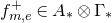



In addition, we have
 $$ f^+_{m,e}\equiv f_{m,e}\equiv a_m \pmod\beta,$$
and since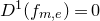 $D^1(f_{m,e})=0$
by construction, we have
$D^1(f_{m,e})=0$
by construction, we have
 $$ D^1(f^+_{m,e}) = \beta^{p^{e+1}-2}D^1(g_{m,e}), $$
which implies the Bockstein differentials.
Using Theorem 4.8, we can compute $\operatorname{gr}_\beta\operatorname{Ext}_{\Gamma_\ast}(A_\ast)$
, the associated graded group with respect to the
$\operatorname{gr}_\beta\operatorname{Ext}_{\Gamma_\ast}(A_\ast)$
, the associated graded group with respect to the $\beta$
-adic filtration. We shall discuss these groups and extension problems in §4.3, but we have a rough description as follows:
$\beta$
-adic filtration. We shall discuss these groups and extension problems in §4.3, but we have a rough description as follows:
-
–
$\operatorname{gr}_\beta\operatorname{Ext}^0$
is
$\mathrm{ku}_\ast$
and is generated by an element represented by the cycle 1; -
–
$\operatorname{gr}_\beta\operatorname{Ext}^1$
is generated by the elements detected by
$p^ea_{p^e}$
for
$e\geq 0$
and
$\lambda_2$
, where these generators are p-torsions and support infinite
$\beta$
-towers; -
–
$\operatorname{gr}_\beta\operatorname{Ext}^2$
is generated by elements detected by
$a_m\lambda_2$
in
$\operatorname{Ext}^1_{\Gamma_\ast}(A_\ast)$
, which is
$p^j\beta^{p^{\operatorname{val}_p(m)-j+1}-2}$
-torsion for each
$0\leq j\leq \operatorname{val}_p(m)$
and
$p^{\operatorname{val}_p(m)+1}$
-torsion.





4.3 Extension problems
We shall resolve the extension problems with respect to the $\beta$
-adic filtration, thereby proving Theorem 1.4.
$\beta$
-adic filtration, thereby proving Theorem 1.4.
Proof of Theorem 1.5. By Theorem 4.8,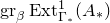 $\operatorname{gr}_\beta\operatorname{Ext}^1_{\Gamma_\ast}(A_\ast)$
is a free
$\operatorname{gr}_\beta\operatorname{Ext}^1_{\Gamma_\ast}(A_\ast)$
is a free $\mathbb Z/p[\beta]$
-module generated by classes represented by the cycles
$\mathbb Z/p[\beta]$
-module generated by classes represented by the cycles $\sigma^2b_1,\sigma^2t_1,\sigma^2t_2,\dots$
From the following differentials in
$\sigma^2b_1,\sigma^2t_1,\sigma^2t_2,\dots$
From the following differentials in $\operatorname{CB}_{\Gamma_\ast}(A_\ast)$
,
$\operatorname{CB}_{\Gamma_\ast}(A_\ast)$
,
 \begin{align*} D^0(\sigma^2 v_{e+1}) &= p\sigma^2 t_{e+1}+\beta^{p^{e+1}-p^e}\sigma^2 t_e,\\ D^0(\sigma^2 x_{p-1}) &= p\sigma^2 t_1 + \delta'\beta^{p-2}\sigma^2 b_1,\end{align*}
we can see that $\operatorname{Ext}^1_{\Gamma_\ast}(A_\ast)$
is isomorphic to
$\operatorname{Ext}^1_{\Gamma_\ast}(A_\ast)$
is isomorphic to $F_p^\wedge$
, defined in §1.2, by identifying the class in
$F_p^\wedge$
, defined in §1.2, by identifying the class in $\operatorname{Ext}^1$
represented by
$\operatorname{Ext}^1$
represented by $\sigma^2 t_e$
with
$\sigma^2 t_e$
with $(\beta^{p^e-2}/f(p^e-2))\in F_p^\wedge$
up to a p-adic unit.
$(\beta^{p^e-2}/f(p^e-2))\in F_p^\wedge$
up to a p-adic unit.
Next, let us describe the extension problems in $\operatorname{Ext}^2_{\Gamma_\ast}(A_\ast)$
. From Theorem 4.8, we see that the class
$\operatorname{Ext}^2_{\Gamma_\ast}(A_\ast)$
. From Theorem 4.8, we see that the class $p^ja_m\lambda_2\in\operatorname{Ext}^1_{\Gamma_\ast}(A_\ast/\beta)$
is hit by the Bockstein differential
$p^ja_m\lambda_2\in\operatorname{Ext}^1_{\Gamma_\ast}(A_\ast/\beta)$
is hit by the Bockstein differential
 $$ d_{p^{\operatorname{val}_p(m)-j+1}-2}(p^{\operatorname{val}_p(m)-j}a_{m+p^{\operatorname{val}_p(m)-j}}). $$
From the proof of that theorem, we see that the class $p^ja_m\lambda_2$
can be lifted to a
$p^ja_m\lambda_2$
can be lifted to a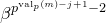 $\beta^{p^{\operatorname{val}_p(m)-j+1}-2}$
-torsion class
$\beta^{p^{\operatorname{val}_p(m)-j+1}-2}$
-torsion class $h_{m,j}\in\operatorname{Ext}^1_{\Gamma_\ast}(A_\ast)$
represented by the cycle
$h_{m,j}\in\operatorname{Ext}^1_{\Gamma_\ast}(A_\ast)$
represented by the cycle
 $$ D^1(g_{m+p^{\operatorname{val}_p(m)-j},\operatorname{val}_p(m)-j}).$$
Let $d=\operatorname{val}_p(m)$
and let j be an integer such that
$d=\operatorname{val}_p(m)$
and let j be an integer such that $0\leq j<d$
. Then, let
$0\leq j<d$
. Then, let $\varepsilon_1,\dots,\varepsilon_{d-j}$
be the sequence defined in Equation (4.3) for the pair
$\varepsilon_1,\dots,\varepsilon_{d-j}$
be the sequence defined in Equation (4.3) for the pair $(m+p^{d-j},d-j)$
. If, in addition
$(m+p^{d-j},d-j)$
. If, in addition $j<d-1$
, then let
$j<d-1$
, then let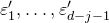 $\varepsilon_1',\dots,\varepsilon_{d-j-1}'$
be the sequence for the pair
$\varepsilon_1',\dots,\varepsilon_{d-j-1}'$
be the sequence for the pair $(m+p^{d-j-1},d-j-1)$
.
$(m+p^{d-j-1},d-j-1)$
.
Case 1. If $j<d-1$
, we have
$j<d-1$
, we have
 \begin{align*} &pf_{m+p^{d-j},d-j} - \frac{\varepsilon_{d-j}}{\varepsilon_{d-j-1}'} \beta^{p^{d-j}(p-1)}f_{m+p^{d-j-1},d-j-1}\\ &\quad=\frac{1}{p^{\operatorname{val}_p(m+p^{d-j})-d+j}}D^0(y^{(m+p^{d-j})/p}) \\ &\qquad+ \frac1p\beta^{p^{d-j}(p-1)}\bigg(\varepsilon_1D^0(y^{m/p}\sigma^2v_{d-j})-\frac{\varepsilon_{d-j}}{\varepsilon_{d-j-1}'}D^0(y^{(m+p^{d-j-1})/p})\bigg)\\ &\qquad+\sum_{k=1}^{d-j-1}\frac{1}{p^{k+1}}\beta^{p^{d-j+1}-p^{d-j-k}}\bigg(\varepsilon_{k+1} - \frac{\varepsilon_{d-j}}{\varepsilon_{d-j-1}'}\varepsilon_k'\bigg)D^0(y^{m/p}\sigma^2 x_{p^{d-j-k}-1}). \end{align*}
We shall show that this is integral, i.e. an element of $A_\ast\otimes\Gamma_\ast$
, possibly except for the first term. For the second term, we have
$A_\ast\otimes\Gamma_\ast$
, possibly except for the first term. For the second term, we have
 $$ D(y^{(m+p^{d-j-1})/p}) \equiv \delta_{d-j-2} D(y^{m/p}\sigma^2 v_{d-j})\pmod p, $$
so that we need to show
 $$ \varepsilon_1 - \frac{\varepsilon_{d-j}}{\varepsilon_{d-j-1}'}\delta_{d-j-2} \equiv 0\pmod p. $$
This is true since we have
 $$ \varepsilon_1 - \frac{\varepsilon_{d-j}}{\varepsilon_{d-j-1}'}\delta_{d-j-2} \equiv\varepsilon_1 + \frac{\varepsilon_1}{\varepsilon_{1}'}\delta_{d-j-2}\pmod p $$
by Lemma 4.10 and
 $$ \varepsilon_1' + \delta_{d-j-2} = \delta_{d-j-2}\bigg(-\frac{m+p^{d-j-1}}{p^{d-j-1}}+1\bigg) \equiv 0\pmod p $$
by Lemma 4.3. Next, for the summation part, we wish to show that
 $$ \varepsilon_{k+1} \equiv \frac{\varepsilon_{d-j}}{\varepsilon_{d-j-1}'}\varepsilon_k'\pmod{p^{k+1}}, $$
and this follows from Lemma 4.10. Therefore, we have proved that
 \begin{align} &pf_{m+p^{d-j},d-j} - \frac{\varepsilon_{d-j}}{\varepsilon_{d-j-1}'} \beta^{p^{d-j}(p-1)}f_{m+p^{d-j-1},d-j-1} \end{align}
 \begin{align} &\quad = \frac{1}{p^{\operatorname{val}_p(m+p^{d-j})-d+j}}D^0(y^{(m+p^{d-j})/p}) + (\text{integral element}). \end{align}
We divide into three cases.
Case 1-1. If $\operatorname{val}_p(m+p^{d-j})=d-j$
, then the whole right-hand side of Equation (4.4) is integral. In this case, we see that
$\operatorname{val}_p(m+p^{d-j})=d-j$
, then the whole right-hand side of Equation (4.4) is integral. In this case, we see that
 \begin{align*} pg_{m+p^{d-j},d-j} - \frac{\varepsilon_{d-j}}{\varepsilon_{d-j-1}'} g_{m+p^{d-j-1},d-j-1} \end{align*}
is integral, so that by taking $D^1$
, we have
$D^1$
, we have
 $$ ph_{m,j} = h_{m,j+1} $$
in $\operatorname{Ext}^2_{\Gamma_\ast}(A_\ast)$
up to a p-adic unit.
$\operatorname{Ext}^2_{\Gamma_\ast}(A_\ast)$
up to a p-adic unit.
Case 1-2. If $m=p^d(p-1)$
and
$m=p^d(p-1)$
and $j=0$
, then from the proof of Theorem 4.8(a)
$j=0$
, then from the proof of Theorem 4.8(a)
 $$ \frac{D^0(y^{p^d})}{p} = \delta_d\beta^{p^{d+2}-p^{d+1}}\frac{\sigma^2 t_{e+1}}p + \text{(integral element)}. $$
Therefore,
 $$ pg_{p^{d+1},d} - \frac{\varepsilon_{d}}{\varepsilon_{d-1}'} g_{m+p^{d-1},d-1} - \delta_d\beta^{p^{d+2}-2p^{d+1}+2}\frac{\sigma^2 t_{e+1}}{p}$$
is integral, and by taking $D^1$
, we obtain
$D^1$
, we obtain
 $$ ph_{p^d(p-1),0} = h_{p^d(p-1),1}. $$
Case 1-3. The remaining case is when $\operatorname{val}_p(m+p^{d-j})\gt d-j$
but not
$\operatorname{val}_p(m+p^{d-j})\gt d-j$
but not $(m,j)\neq(p^d(p-1),0)$
. This can happen only if
$(m,j)\neq(p^d(p-1),0)$
. This can happen only if $j=0$
. In this case, we have
$j=0$
. In this case, we have
 $$ f_{m+p^d,d+1} = \frac{1}{p^{\operatorname{val}_p(m+p^d)-d}}D^0(y^{(m+p^d)/p}) + \beta^{p^{d+2}-p^{d+1}}\times\text{(cycle)}, $$
where (cycle) means some cycle in $A_\ast\otimes\Gamma_\ast[p^{-1}]$
. Comparing with Equation (4.4), we see that
$A_\ast\otimes\Gamma_\ast[p^{-1}]$
. Comparing with Equation (4.4), we see that
 $$ pg_{m+p^d,d} - \frac{\varepsilon_{d}}{\varepsilon_{d-1}'}g_{m+p^{d-1},d-1} - \beta^{p^{d+2}-p^{d+1}} g_{m+p^d,d+1} + \beta^{p^{d+2}-2p^{d+1}+2} \times\text{(cycle)} $$
is integral. Taking $D^1$
, we have
$D^1$
, we have
 $$ ph_{m,0} = h_{m,1} + \beta^{p^{d+2}-p^{d+1}}h_{m-p^d(p-1),d'-d-1}, $$
where $d'=\operatorname{val}_p(m-p^d(p-1))$
. This completes the proof when
$d'=\operatorname{val}_p(m-p^d(p-1))$
. This completes the proof when $j<d-1$
.
$j<d-1$
.
Case 2 If $j=d-1$
, then we have
$j=d-1$
, then we have
 \begin{align*} &pf_{m+p,1} - c\beta^{p(p-1)}f_{m+1,0} \\ &\quad = \frac{1}{p^{\operatorname{val}_p(m+p)-1}} D^0(y^{(m+p)/p}) \\ &\qquad + \frac1p\beta^{p(p-1)}(\varepsilon_1D^0(y^{m/p}\sigma^2 x_{p-1})-cD^0((\sigma^2 x_{p-1})^{m+1})) \end{align*}
and we can choose a p-adic unit c so that
 $$ \frac1p\beta^{p(p-1)}(\varepsilon_1D^0(y^{m/p}\sigma^2 x_{p-1})-cD^0((\sigma^2 x_{p-1})^{m+1})) $$
is $\beta^{2p^2-3p}$
times a cycle by the definition of y. The rest of the argument is similar to the previous cases.
$\beta^{2p^2-3p}$
times a cycle by the definition of y. The rest of the argument is similar to the previous cases.
Case 3. For $j=d$
, we have
$j=d$
, we have
 $$ pf_{m+1,0} = \frac{1}{p^{\operatorname{val}_p(m+1)}}D^0((\sigma^2 x_{p-1})^{m+1})$$
and the rest of the argument is similar to the previous cases.
This completes the proof of the description of $\operatorname{Ext}_{\Gamma_\ast}(A_\ast)$
. The rest of the statement immediately follows.
$\operatorname{Ext}_{\Gamma_\ast}(A_\ast)$
. The rest of the statement immediately follows.
5. Integral homotopy via fracture square
In this section, we shall compute the homotopy groups of $\operatorname{THH}(\mathrm{ku})$
, thereby proving Theorem 1.4, by assembling the p-complete homotopy groups of
$\operatorname{THH}(\mathrm{ku})$
, thereby proving Theorem 1.4, by assembling the p-complete homotopy groups of $\operatorname{THH}(\mathrm{ku})$
. Recall that
$\operatorname{THH}(\mathrm{ku})$
. Recall that $\operatorname{THH}(\mathrm{ku})$
splits into a direct sum
$\operatorname{THH}(\mathrm{ku})$
splits into a direct sum
 $$ \operatorname{THH}(\mathrm{ku}) = \mathrm{ku} \oplus\overline{\operatorname{THH}(\mathrm{ku})}.$$
Let $X=\overline{\operatorname{THH}(\mathrm{ku})}$
. Then, we can compute the homotopy groups of X using the arithmetic fracture square
$X=\overline{\operatorname{THH}(\mathrm{ku})}$
. Then, we can compute the homotopy groups of X using the arithmetic fracture square

which is a pullback. Equivalently, there is a cofiber sequence
 $$ X\to (X\otimes\mathbb Q)\oplus \Big(\prod_{p}X_p^\wedge\Big) \to \Big(\prod_{p}X_p^\wedge\Big)\otimes\mathbb Q. $$
Lemma 5.1. The rational homotopy groups of $\operatorname{THH}(\mathrm{ku})$
are
$\operatorname{THH}(\mathrm{ku})$
are
 $$ \pi_\ast(\operatorname{THH}(\mathrm{ku})\otimes\mathbb Q) = \mathbb Q[\beta]\oplus\Sigma^3\mathbb Q[\beta] $$
as a $\mathbb Q[\beta]$
-module. The second summand is generated by
$\mathbb Q[\beta]$
-module. The second summand is generated by $\sigma b_1$
, where
$\sigma b_1$
, where $b_1$
denotes the image of
$b_1$
denotes the image of $b_1\in\mathrm{MU}_\ast\mathrm{MU}$
in
$b_1\in\mathrm{MU}_\ast\mathrm{MU}$
in $\mathrm{ku}_\ast\mathrm{ku}$
.
$\mathrm{ku}_\ast\mathrm{ku}$
.
Proof. The $E_2$
-page of the Bökstedt spectral sequence
$E_2$
-page of the Bökstedt spectral sequence
 $$ E_2 = \operatorname{HH}_\ast(\pi_\ast(\mathrm{ku}\otimes\mathbb Q)/\mathbb Q) \Rightarrow \pi_\ast(\operatorname{THH}(\mathrm{ku})\otimes\mathbb Q) $$
is
 $$ E_2 = \Lambda_{\mathbb Q[\beta]}(\sigma(\beta_1-\beta_2)),$$
where $\beta_1,\beta_2$
are the two copies of
$\beta_1,\beta_2$
are the two copies of $\beta$
in
$\beta$
in $\mathbb Q[\beta]\otimes_{\mathbb Q}\mathbb Q[\beta]$
. The spectral sequence degenerates since there is no room for any differential, and the conclusion follows from the observation that
$\mathbb Q[\beta]\otimes_{\mathbb Q}\mathbb Q[\beta]$
. The spectral sequence degenerates since there is no room for any differential, and the conclusion follows from the observation that $\sigma(\beta_1-\beta_2)$
detects
$\sigma(\beta_1-\beta_2)$
detects $\sigma b_1$
rationally.
$\sigma b_1$
rationally.
Proof of Theorem 1.4. We shall prove that the map
 \begin{equation} (X\otimes\mathbb Q)\oplus \Big(\prod_{p}X_p^\wedge\Big) \to \Big(\prod_{p}X_p^\wedge\Big)\otimes\mathbb Q \end{equation}
in the arithmetic fracture square is a surjection on homotopy groups and compute the kernel.
At even degrees, Equation (5.1) is
 $$ 0\oplus\bigoplus_p T(p) \to 0,$$
so that the even homotopy group of X is $\bigoplus_pT(p)$
.
$\bigoplus_pT(p)$
.
Next, we note that in the expression
 $$ \operatorname{THH}_\ast(\mathrm{ku})_p^\wedge = \mathbb Z_p[\beta]\oplus F_p^\wedge\oplus T(p) $$
of Theorem 1.5, the generator of $\operatorname{THH}_3(\mathrm{ku})_p^\wedge$
, i.e. the lowest-degree generator of
$\operatorname{THH}_3(\mathrm{ku})_p^\wedge$
, i.e. the lowest-degree generator of $F_p^\wedge$
, is
$F_p^\wedge$
, is $\sigma b_1$
. This follows from the proof of Theorem 1.5 in §4.3 combined with Remark 3.13.
$\sigma b_1$
. This follows from the proof of Theorem 1.5 in §4.3 combined with Remark 3.13.
Then, at an odd degree, say $2k+3$
, Equation (5.1) is
$2k+3$
, Equation (5.1) is
 $$ \mathbb Q \oplus \prod_p\mathbb Z_p\to\Big(\prod_p\mathbb Z_p\Big)\otimes\mathbb Q $$
where $\mathbb Q$
on the left-hand side is generated by
$\mathbb Q$
on the left-hand side is generated by $\beta^k\sigma b_1$
and the
$\beta^k\sigma b_1$
and the $\mathbb Z_p$
on both sides are generated by
$\mathbb Z_p$
on both sides are generated by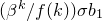 $(\beta^k/f(k))\sigma b_1$
. This is the fracture square for the ordinary ring
$(\beta^k/f(k))\sigma b_1$
. This is the fracture square for the ordinary ring $\mathbb Q$
. Therefore, it is surjective and the kernel is
$\mathbb Q$
. Therefore, it is surjective and the kernel is $\mathbb Z$
generated by
$\mathbb Z$
generated by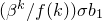 $(\beta^k/f(k))\sigma b_1$
.
$(\beta^k/f(k))\sigma b_1$
.
6. Further questions
It would be interesting if the descent spectral sequence for $\operatorname{THH}(R)\to\operatorname{THH}(R/\mathrm{MU})$
were to degenerate for more general R. When
$\operatorname{THH}(R)\to\operatorname{THH}(R/\mathrm{MU})$
were to degenerate for more general R. When $R=\mathrm{BP}\langle n\rangle$
is a
$R=\mathrm{BP}\langle n\rangle$
is a $\mathbb E_3$
-MU-algebra, [Reference Hahn and WilsonHW22, Proposition 6.1.6] implies that
$\mathbb E_3$
-MU-algebra, [Reference Hahn and WilsonHW22, Proposition 6.1.6] implies that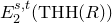 $E_2^{s,t}(\operatorname{THH}(R))$
is concentrated in
$E_2^{s,t}(\operatorname{THH}(R))$
is concentrated in $0\leq s\leq n+1$
, so that the degeneracy is not immediate as in Corollary 4.2. However, since the descent spectral sequence for
$0\leq s\leq n+1$
, so that the degeneracy is not immediate as in Corollary 4.2. However, since the descent spectral sequence for $R=\mathrm{MU}$
degenerates at the
$R=\mathrm{MU}$
degenerates at the $E_2$
-page, the following conjecture would imply the degeneracy for
$E_2$
-page, the following conjecture would imply the degeneracy for $R=\mathrm{BP}\langle n\rangle$
. Note that the assumption that R is a
$R=\mathrm{BP}\langle n\rangle$
. Note that the assumption that R is a $\mathbb E_3$
-MU-algebra is needed to ensure that
$\mathbb E_3$
-MU-algebra is needed to ensure that $\operatorname{THH}_\ast(R/\mathrm{MU})$
is a commutative ring.
$\operatorname{THH}_\ast(R/\mathrm{MU})$
is a commutative ring.
Conjecture 6.1. Suppose that we have $\mathrm{BP}\langle n\rangle$
with an
$\mathrm{BP}\langle n\rangle$
with an $\mathbb E_3$
-MU-algebra structure, which exists by [Reference Hahn and WilsonHW22]. Let
$\mathbb E_3$
-MU-algebra structure, which exists by [Reference Hahn and WilsonHW22]. Let $E_2(\operatorname{THH}(\mathrm{MU}))$
and
$E_2(\operatorname{THH}(\mathrm{MU}))$
and $E_2(\operatorname{THH}(\mathrm{BP}\langle n\rangle))$
be the
$E_2(\operatorname{THH}(\mathrm{BP}\langle n\rangle))$
be the $E_2$
-page of the descent spectral sequence for
$E_2$
-page of the descent spectral sequence for $\operatorname{THH}(\mathrm{MU})\to\operatorname{THH}(\mathrm{MU}/\mathrm{MU})$
and
$\operatorname{THH}(\mathrm{MU})\to\operatorname{THH}(\mathrm{MU}/\mathrm{MU})$
and $\operatorname{THH}(\mathrm{BP}\langle n\rangle)\to\operatorname{THH}(\mathrm{BP}\langle n\rangle/\mathrm{MU})$
. Then,
$\operatorname{THH}(\mathrm{BP}\langle n\rangle)\to\operatorname{THH}(\mathrm{BP}\langle n\rangle/\mathrm{MU})$
. Then,
 $$ E_2^{s,t}(\operatorname{THH}(\mathrm{MU}))\to E_2^{s,t}(\operatorname{THH}(\mathrm{BP}\langle n\rangle)) $$
is surjective for $0\leq s\leq n$
.
$0\leq s\leq n$
.
Theorem 4.8(a) shows that the conjecture is true for ku instead of $\mathrm{BP}\langle 1\rangle$
, i.e. the map
$\mathrm{BP}\langle 1\rangle$
, i.e. the map $E_2^{s,t}(\operatorname{THH}(\mathrm{MU}))\to E_2^{s,t}(\operatorname{THH}(\mathrm{ku}))$
is surjective for
$E_2^{s,t}(\operatorname{THH}(\mathrm{MU}))\to E_2^{s,t}(\operatorname{THH}(\mathrm{ku}))$
is surjective for $0\leq s\leq 1$
. Similar computations can be done to show that the conjecture is true for
$0\leq s\leq 1$
. Similar computations can be done to show that the conjecture is true for $0\leq s\leq 1$
and any n.
$0\leq s\leq 1$
and any n.
Acknowledgements
I would like to thank Jeremy Hahn for suggesting the problem and for helpful conversations in the course of this work. I would also like to thank Ben Antieau, Sanath Devalapurkar, and Ishan Levy for helpful conversations related to the work. I would like to thank the anonymous referee for comments on an earlier draft that have improved the exposition.
Conflicts of interest
None.
Financial support
This work was partially supported by a fellowship from the Department of Mathematics, MIT.
Journal information
Compositio Mathematica is owned by the Foundation Compositio Mathematica and published by the London Mathematical Society in partnership with Cambridge University Press. All surplus income from the publication of Compositio Mathematica is returned to mathematics and higher education through the charitable activities of the Foundation, the London Mathematical Society and Cambridge University Press.


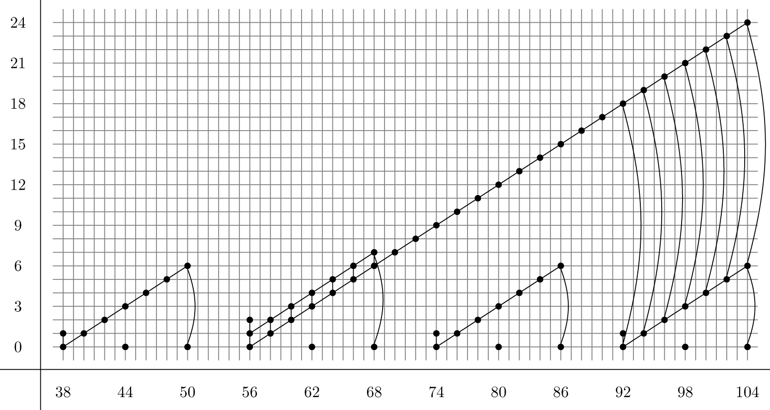

 Open access

