





1. Introduction
Describing coating flow over a solid is a theoretical challenge, yet endlessly appealing because of the many simple phenomena that involve these kinds of flows: we withdraw spoons covered in honey from a jar, coat strawberries in chocolate, dip and remove a paintbrush from a bucket, lift ourselves out of the water at the swimming pool, and take pictures with film made of a light-sensitive chemical coated over a transparent strip. In general, in dip coating processes, the film thickness  $h_0$ coated on objects pulled from a bath of viscous liquid depends on the capillary number $Ca = {\eta v_0}/{\gamma }$, which describes the balance between viscous and capillary forces, where $v_0$ is the pulling velocity, $\eta$ is the liquid's dynamic viscosity, and $\gamma$ is the liquid's surface tension. The initial model for dip coating a Newtonian liquid over a smooth, flat plate at small $Ca$ gives the relation (Landau & Levich Reference Landau and Levich1942; Derjaguin Reference Derjaguin1943; Wilson Reference Wilson1982)
 \begin{equation} h_0 = 0.94 a\,Ca^{{2}/{3}}, \end{equation}
where  $a = \sqrt {\gamma /(\rho g)}$ is the capillary length, $\rho$ is the liquid's density, and $g$ is the magnitude of gravitational acceleration. The model matched earlier experiments of Morey (Reference Morey1940), who found $h_0 \sim Ca^{{2}/{3}}$.
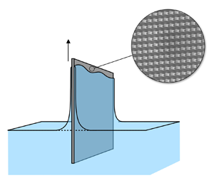
The model (1.1) has been extended to include corrections accounting for gravity and inertia at larger  $Ca$ (Spiers, Subbaraman & Wilkinson Reference Spiers, Subbaraman and Wilkinson1974; de Ryck & Quéré Reference de Ryck and Quéré1998). Theoretical and experimental extensions have also been made with regard to the object coated – including tilted plates (Wilson Reference Wilson1982; Benilov & Zubkov Reference Benilov and Zubkov2008), horizontal and vertical cylinders (White & Tallmadge Reference White and Tallmadge1966; Spiers et al. Reference Spiers, Subbaraman and Wilkinson1974; Wilson Reference Wilson1982; Quéré Reference Quéré1999), compliant surfaces (Kajiya et al. Reference Kajiya, Brunet, Royon, Daerr, Receveur and Limat2014; Bertin et al. Reference Bertin, Snoeijer, Raphaël and Salez2022), and rough surfaces (Krechetnikov & Homsy Reference Krechetnikov and Homsy2005; Seiwert, Clanet & Quéré Reference Seiwert, Clanet and Quéré2011; Sathyanath, Aarthi & Kalpathy Reference Sathyanath, Aarthi and Kalpathy2020) – as well as the liquid properties, as reviewed in Rio & Boulogne (Reference Rio and Boulogne2017). Given the multitude of realistic situations in which a surface to be coated is rough or porous, rather than smooth (Stauffer, Hajnal & Gendzwill Reference Stauffer, Hajnal and Gendzwill1976; Barthlott & Neinhuis Reference Barthlott and Neinhuis1997; Neinhuis & Barthlott Reference Neinhuis and Barthlott1997; Devauchelle, Josserand & Zaleski Reference Devauchelle, Josserand and Zaleski2007; Nong & Anderson Reference Nong and Anderson2010), we focus our attention on thin film flow over a rough surface pulled from a liquid bath (figure 1). The film profile is $h = h(z)$, and in the dynamic meniscus region (region II), the profile tends towards a flat film of constant thickness $h \to h_0$ as $z \to \infty$. Although initial progress has been made to characterize the effect of roughness on the film thickness (Aradian, Raphaël & de Gennes Reference Aradian, Raphaël and de Gennes2000; Krechetnikov & Homsy Reference Krechetnikov and Homsy2005; Seiwert Reference Seiwert2010; Seiwert et al. Reference Seiwert, Clanet and Quéré2011; Sathyanath et al. Reference Sathyanath, Aarthi and Kalpathy2020), at present we lack a general model capable of predicting film thickness coated on an arbitrary periodic roughness pattern.
Dip coating system. (a) A solid plate is pulled at constant velocity  $\boldsymbol {v} = v_0 \hat {\boldsymbol {z}}$ from a liquid bath having density $\rho$, surface tension $\gamma$, and dynamic viscosity $\eta$, where $\boldsymbol {v}$ is directed opposite to the direction of gravitational acceleration $\boldsymbol {g}$. The plate is rough, with a periodic texture pattern. To model the rough surface, we apply an equivalent boundary condition to a flat equivalent surface $\mathbb {ES}$ that is placed a distance $d_{\mathbb {ES}}$ from the bottom of the roughness. The thin film on the plate forms three regions: a flat film (region I) is connected to a static meniscus (region III) by a dynamic meniscus (region II). We wish to know the limiting film thickness $h(z) = h_0$ in the flat film region. (b) The film thickness $h(z)$ as a function of the coordinate $z$ along the plate.

At large  $Ca$, the film thickness coated on a rough plate is found to be modelled well by (1.1), while experiments demonstrate that at small $Ca$, surface roughness significantly increases film thickness compared to the case of a smooth plate (Krechetnikov & Homsy Reference Krechetnikov and Homsy2005; Seiwert et al. Reference Seiwert, Clanet and Quéré2011). The physical reason for this increase is that the roughness introduces a minimum film thickness due to viscous resistance to liquid flow against the additional solid walls or pore-like features, which have a greater area compared to the flat case (Seiwert et al. Reference Seiwert, Clanet and Quéré2011). For a rough plate, the film thickness no longer goes to zero as $Ca \to 0$ as predicted by (1.1); instead, experiments demonstrate that a small film remains trapped within the rough features due to viscous resistance, such that $h_0 \to h_{min}$ as $Ca \to 0$. The scale of this minimum thickness is $h_{min} \sim r$, with $r$ being the typical peak-to-valley scale of the roughness. Seiwert et al. (Reference Seiwert, Clanet and Quéré2011) thus divide the film into two regions: a trapped fluid region located within the roughness features, and a free film region outside, separated by a flat plane located at the peak of the roughness features.
Motivated by such physical reasoning, Krechetnikov & Homsy (Reference Krechetnikov and Homsy2005), Liao, Li & Wei (Reference Liao, Li and Wei2013) and Sathyanath et al. (Reference Sathyanath, Aarthi and Kalpathy2020) proposed a model for rough dip coating that would replace the no-slip boundary condition at the rough wall by a slip boundary condition at a fictitious flat boundary plane at the peak of the roughness features. Such a model is sensible if we consider that at the boundary plane, we find a mix of solid and fluid patches, meaning that at the boundary there is a non-zero slip velocity (Beavers & Joseph Reference Beavers and Joseph1967). Introducing slip has been used successfully to model experimentally observed velocity profiles in channels with rough walls (Lauga & Stone Reference Lauga and Stone2003; Maali & Bhushan Reference Maali and Bhushan2012), where flow velocities are similar to those in small- $Ca$ dip coating experiments. However, Seiwert et al. (Reference Seiwert, Clanet and Quéré2011) found that a slip model was insufficient to explain their observation of a constant minimum film thickness ( $h_0 = h_{min}$) with no free film coated below a critical capillary number $Ca < Ca_c$; the slip model overestimated the experimentally observed free film thickness. A modified model was developed that proposed to augment the slip velocity by considering porous flow through the rough layer, but it lacked experimental comparison (Devauchelle et al. Reference Devauchelle, Josserand and Zaleski2007). Instead of using a slip model, Seiwert et al. (Reference Seiwert, Clanet and Quéré2011) proposed to model the system as two layers of liquid, where the trapped-fluid region is replaced by a liquid of higher viscosity $\eta ^* > \eta$, and subsequently solve for $h_0$. When $\eta ^*$ was used as a fitting parameter to the experimental data, this ‘two-layer model’ predicted the formation of a trapped film and the total depletion of the free film for $Ca < Ca_c$.
Despite the successes of prior modelling efforts (Krechetnikov & Homsy Reference Krechetnikov and Homsy2005; Seiwert et al. Reference Seiwert, Clanet and Quéré2011; Liao et al. Reference Liao, Li and Wei2013; Sathyanath et al. Reference Sathyanath, Aarthi and Kalpathy2020), these models are not fully predictive since closure of the problem requires experimental data to fit either the slip length  $\mathcal {L}$ or the viscosity increase parameter $\eta ^*$. Here, we develop a model that provides further insight into the physical mechanism by which the microstructure affects the macroscopic flow, and in doing so, present a predictive model for the film thickness coated on rough surfaces by a viscous liquid. The key factor enabling the predictability of the model employed in the present work stems from the use of a homogenization technique (Hornung Reference Hornung1997; Espedal, Fasano & Mikelić Reference Espedal, Fasano and Mikelić2000; Mei & Vernescu Reference Mei and Vernescu2010), which allows us to derive effective macroscopic properties of a surface from its microscopic structure. The upscaling procedure involves taking a spatial average of microscopic flow quantities describing the flow around a single microscopic roughness feature to compute effective macroscopic properties. Properties upscaled from the microstructure can then be applied to the macroscopic problem via an interface condition imposed over a fictitious flat surface called the ‘equivalent surface’ ( $\mathbb {ES}$ in figure 1) placed between the trapped liquid layer and the free film.
Homogenization can be used to analyse fluid–solid interaction phenomena where there is a separation of scales between the typical microscopic roughness size and the whole macroscopic system size (Mei & Vernescu Reference Mei and Vernescu2010). The large scale may be given by the size of a macroscopic object (such as the radius of a sphere with a rough surface) or by the scale of the flow domain (such as the height of a channel) (Zampogna & Bottaro Reference Zampogna and Bottaro2016; Zampogna, Magnaudet & Bottaro Reference Zampogna, Magnaudet and Bottaro2019; Sudhakar et al. Reference Sudhakar, Lācis, Pasche and Bagheri2021). Thus homogenization has been employed extensively to calculate the effective flow of an incompressible fluid in domains with no free interface, such as through porous and poroelastic media (Levy & Sanchez-Palencia Reference Levy and Sanchez-Palencia1975; Carraro et al. Reference Carraro, Goll, Marciniak-Czochra and Mikelić2015; Zampogna & Bottaro Reference Zampogna and Bottaro2016; Lācis & Bagheri Reference Lācis and Bagheri2017; Lācis, Zampogna & Bagheri Reference Lācis, Zampogna and Bagheri2017; Sudhakar et al. Reference Sudhakar, Lācis, Pasche and Bagheri2021; Strohbeck, Eggenweiler & Rybak Reference Strohbeck, Eggenweiler and Rybak2023), over rough surfaces (Jiménez Bolaños & Vernescu Reference Jiménez Bolaños and Vernescu2017; Zampogna et al. Reference Zampogna, Magnaudet and Bottaro2019; Lācis et al. Reference Lācis, Sudhakar, Pasche and Bagheri2020; Naqvi & Bottaro Reference Naqvi and Bottaro2021), and across periodic and weakly periodic microstructured permeable surfaces (Zampogna & Gallaire Reference Zampogna and Gallaire2020; Ledda et al. Reference Ledda, Boujo, Camarri, Gallaire and Zampogna2021; Zampogna, Ledda & Gallaire Reference Zampogna, Ledda and Gallaire2022). Bottaro & Naqvi (Reference Bottaro and Naqvi2020) have shown that the flow at an interface between a free-fluid region and a rough surface is described by the slip tensor  $\boldsymbol {\mathcal {L}}$ and interface permeability tensor $\boldsymbol {\mathcal {K}}^{itf}$ (see also Naqvi & Bottaro Reference Naqvi and Bottaro2021). Following their work, in contrast to the slip models (Krechetnikov & Homsy Reference Krechetnikov and Homsy2005; Sathyanath et al. Reference Sathyanath, Aarthi and Kalpathy2020), the boundary condition that we use considers both slip due to fluid patches at the equivalent surface (through $\boldsymbol {\mathcal {L}}$) and an excess tangential velocity driven by a pressure gradient over the rough layer (through $\boldsymbol {\mathcal {K}}^{itf}$). We employ a boundary condition of this form to model the thin film flow. Using the homogenization framework to compute $\boldsymbol {\mathcal {L}}$ and $\boldsymbol {\mathcal {K}}^{itf}$ for any surface with a periodic roughness pattern (Zampogna et al. Reference Zampogna, Magnaudet and Bottaro2019; Bottaro & Naqvi Reference Bottaro and Naqvi2020; Naqvi & Bottaro Reference Naqvi and Bottaro2021), we can predict the coated film thickness without any fitting parameter.
We first present the solution for the coated film thickness using a homogenized boundary condition to model the rough surface (§ 2). Using the effective macroscopic properties of each surface derived from its microstructure, we solve the macroscopic lubrication equations and predict the coated film thickness. We present the experimental methods in § 3, where we describe the fabrication of micropillar arrays, as well as the interferometry technique used to measure  $h_0$. The model is compared to experimental data (§ 4), and finally we discuss our results and their implications for further study of thin film flow over rough surfaces (§ 5).
2. Model of thin film flow over a porous bed
The dip coating system is illustrated in figure 1, where a rough plate is pulled continuously from a liquid with density  $\rho$, surface tension $\gamma$, and dynamic viscosity $\eta$. Three regions are observed: a flat film (region I) is connected by a dynamic meniscus (region II) to a static meniscus where the film meets the bath (region III). We consider the film profile $h(z)$ indicated in figure 1(b), and in particular aim to find its limiting value $h \to h_0$ as $z \to \infty$.
We model the system by considering the flow of a thin liquid film over a rough or porous plate. The challenge in modelling such a system arises, first, because of the complex shape of the rough or porous surface, which is difficult to address by an analytical solution. The second challenge is the multiscale nature of the problem: the roughness amplitude  $h_p$ may be much smaller than the film thickness $h_0$, which makes a direct numerical simulation computationally expensive. In addition, we desire to develop a general model for thin film flow over surfaces with arbitrary roughness topography, and we cannot arrive at such insight from seeking a separate numerical solution for each surface texture that we wish to model. The homogenization method is an attractive choice for addressing these problems, because it can address arbitrarily complex periodic roughness patterns, yet requires a full numerical solution only within a periodic cell containing a single roughness feature to produce effective parameters for a simplified equivalent boundary condition (Mei & Vernescu Reference Mei and Vernescu2010; Zampogna et al. Reference Zampogna, Magnaudet and Bottaro2019; Bottaro & Naqvi Reference Bottaro and Naqvi2020; Naqvi & Bottaro Reference Naqvi and Bottaro2021). These constant parameters are found by averaging the solution of associated Stokes problems in the microscopic domain (Zampogna et al. Reference Zampogna, Magnaudet and Bottaro2019; Bottaro & Naqvi Reference Bottaro and Naqvi2020; Naqvi & Bottaro Reference Naqvi and Bottaro2021). The resulting boundary condition can be applied in an analytical approach to the full-scale problem, which is treated in a manner similar to the classic analysis for a smooth plate (Landau & Levich Reference Landau and Levich1942).
Before any simplification, our system consists of a Newtonian liquid flowing over a solid surface with arbitrary periodic roughness, which is governed by the Navier–Stokes equations (2.1)–(2.2) subject to the boundary condition that fluid cannot flow through the solid and that fluid velocity tangential to the solid is zero (no-slip). At the liquid–air interface, we apply the no-shear boundary condition and a capillary stress. The model proceeds in three steps. First, we present the governing equations in § 2.1, and after assuming a separation of scales between the texture's periodicity and the film thickness, in § 2.2 we identify a homogenized boundary condition that represents the roughness of the plate yet can be applied at an equivalent flat surface  $\mathbb {ES}$ (see figures 2b,c) instead of the original complex roughness shape. Second, by assuming that the film is thin, we perform a lubrication expansion on the governing equations and boundary conditions: the resulting simplified equations are presented in each respective subsection. Finally, in § 2.3, we solve the resulting equations for the film thickness $h_0$ coated on the plate as a function of velocity $v_0$ and the liquid properties ( $\rho,\gamma,\eta$).
Boundary conditions for (a) smooth and (b,c) rough plates. Velocity profiles are sketched in a reference frame moving with the plate for three conditions: (a) no slip, (b) slip, (c) slip and porous flow. The yellow arrow represents the slip contribution, and the pink arrow represents the contribution from porous flow, driven by a pressure gradient through the rough layer. For a rough surface, the slip contribution is  $O(\epsilon ^0)$ and the porous flow contribution is $O(\epsilon ^1)$ (Naqvi & Bottaro Reference Naqvi and Bottaro2021).

2.1. Governing equations
The rough surfaces are pulled from a Newtonian liquid of density  $\rho$ and dynamic viscosity $\eta$, such that the flow satisfies the three-dimensional incompressible Navier–Stokes equations,
 $$\begin{gather} \frac{\partial \boldsymbol{u}}{\partial t} + (\boldsymbol{u} \boldsymbol{\cdot}\boldsymbol{\nabla}) \boldsymbol{u} =\frac{\eta}{\rho}\,\nabla^2 \boldsymbol{u} - \frac{1}{\rho}\, \boldsymbol{\nabla} p + \boldsymbol{g}, \end{gather}$$
 $$\begin{gather}\boldsymbol{\nabla} \boldsymbol{\cdot} \boldsymbol{u} = 0, \end{gather}$$
where  $\boldsymbol {u} = u_x \hat {\boldsymbol {x}} + u_y \hat {\boldsymbol {y}} + u_z \hat {\boldsymbol {z}}$ is the liquid velocity, $p$ is the pressure, and $\boldsymbol {g} = -g \hat {\boldsymbol {z}}$ ( $g > 0$) is the gravitational acceleration. The operator $\boldsymbol {\nabla }$ is defined as $\boldsymbol {\nabla } = \hat {\boldsymbol {x}} ({\partial }/{\partial x}) + \hat {\boldsymbol {y}} ({\partial }/{\partial y}) + \hat {\boldsymbol {z}} ({\partial }/{\partial z})$. In (2.1), assuming that the system is in steady state, we drop the unsteady term $\partial \boldsymbol {u}/\partial t = 0$. Assuming that velocities are zero in the $y$-direction, we simplify the problem to two dimensions, $x$ and $z$ (see figure 1). We remark that while the assumption $u_y = 0$ is clearly sensible for a case of two-dimensional periodic structures that are invariant in the $y$-direction, such as ridges, it is not obvious that velocities should be zero along $y$ for generic roughness patterns, such as a bed of pillars. Yet as long as the roughness pattern is periodic and isotropic in the $(y,z)$-plane, there is no reason for any symmetry breaking flow along $y$, and we may expect on average that that velocity is zero along $y$. Thus for patterns that satisfy the condition of isotropy in the plane of the plate, this assumption is sensible.
Supposing that a characteristic film thickness scale  $\ell '$ is much smaller than a characteristic scale $\ell ''$ of the interface profile variation along the film surface, we perform a lubrication expansion in the small parameter $\delta = \ell '/\ell ''$, arriving at the leading-order equations (Reynolds Reference Reynolds1886; Oron, Davis & Bankhoff Reference Oron, Davis and Bankhoff1997; Balestra Reference Balestra2018)
 $$\begin{gather} \frac{\partial \tilde{p}}{\partial \tilde{x}} = 0, \end{gather}$$
 $$\begin{gather}\frac{\partial^2 \tilde{u}_z}{\partial \tilde{x}^2} = \frac{\partial \tilde{p}}{\partial \tilde{z}} + \frac{\rho g \ell'^2}{\eta U_z}, \end{gather}$$
where  $\tilde {\cdot }$ denotes dimensionless variables, and lengths and velocities have been normalized by characteristic scales
 \begin{equation} x = \ell' \tilde{x},\quad z = \ell'' \tilde{z},\quad u_x = U_x \tilde{u}_x,\quad u_z = U_z \tilde{u}_z. \end{equation}
The pressure is normalized as
 \begin{equation} p = \frac{\eta U_z}{\delta \ell'}\,\tilde{p} = \frac{\eta U_z}{\ell'^2/\ell''}\,\tilde{p}. \end{equation}
In addition, the liquid velocity normal to the plate is much smaller than its velocity parallel to the plate, so  $U_x \sim \delta U_z$. This relation is required for mass conservation to hold at each order (Oron et al. Reference Oron, Davis and Bankhoff1997). Later, we will require the dimensional forms of (2.3)–(2.4), which are given as
 $$\begin{gather} \frac{\partial p}{\partial x} = 0, \end{gather}$$
 $$\begin{gather}\frac{\eta}{\rho}\,\frac{\partial^2 u_z}{\partial x^2} = \frac{1}{\rho}\,\frac{\partial p}{\partial z} + g. \end{gather}$$
Note that the characteristic scale  $\ell ''$ in our case is of the order of the capillary length $a$, which sets the meniscus scale in region III (figure 1).
2.2. Boundary conditions
2.2.1. Interface condition at the plate
Supposing that the characteristic spacing  $\ell$ between two periodic roughness elements is much smaller than the size of the liquid domain $\ell '$ ( $\epsilon = \ell /\ell ' \ll 1$), we use the homogenized boundary condition described in Bottaro & Naqvi (Reference Bottaro and Naqvi2020), keeping terms up to $O(\epsilon ^2)$. The parameter $\epsilon$ is a separation of scales parameter that is assumed to be small in the homogenization procedure. Before specifying the boundary condition, we must first define a fictitious equivalent surface, denoted $\mathbb {ES}$, where the macroscopic effective condition applies. Similar to Bottaro & Naqvi (Reference Bottaro and Naqvi2020), we define $\mathbb {ES}$ to be a flat plane located at a distance $d_{\mathbb {ES}}$ from the bottom of the roughness features (figure 1a), and select the location $d_{\mathbb {ES}} = h_p$, which means that $\mathbb {ES}$ is located at the interface between the rough layer and the free-fluid region (figures 2b,c). As has been discussed previously (Espedal et al. Reference Espedal, Fasano and Mikelić2000; Marciniak-Czochra & Mikelić Reference Marciniak-Czochra and Mikelić2012), there is some freedom in the choice of the distance $d_{\mathbb {ES}}$: numerical results demonstrate empirically that shifting the equivalent surface position by $O(\epsilon )$ does not significantly change the macroscopic results predicted by a homogenized theory, as the variation of macroscopic results is within $O(\epsilon )$ (Lācis & Bagheri Reference Lācis and Bagheri2017; Zampogna et al. Reference Zampogna, Magnaudet and Bottaro2019). Our choice of $d_\mathbb {ES}$ is based on the assumption that liquid is always trapped within the rough layer, as has been observed in prior experiments (Seiwert et al. Reference Seiwert, Clanet and Quéré2011). In our case, $h_p$ represents a pillar height, but in general, $h_p$ represents the characteristic peak-to-valley scale of the rough layer.
Note that due to the position of  $\mathbb {ES}$, we will later decompose the total film profile $h(z)$ into two parts, $h(z) = h_p + \bar {h}(z)$, where $h_p$ is the known height of the trapped layer, and $\bar {h}(z)$ is the unknown thickness of the free film above $\mathbb {ES}$: solving the macroscopic model will give the asymptotic free film thickness $\bar {h}_0 \equiv \bar {h}(z \to \infty )$ measured with respect to $\mathbb {ES}$. The total film thickness will then be $h_0 = h_p + \bar {h}_0$. Having selected the equivalent surface's position, the boundary condition at $\mathbb {ES}$ is
 $$\begin{gather} u_x(x = 0, z) ={-} \mathcal{K}^{itf}\,\frac{\partial}{\partial z} \left(\frac{\partial u_z}{\partial x} + \frac{\partial u_x}{\partial z}\right), \end{gather}$$
 $$\begin{gather}u_z(x = 0, z) = v_0 + \mathcal{L} \left(\frac{\partial u_z}{\partial x} + \frac{\partial u_x}{\partial z}\right) + \frac{\mathcal{K}^{itf}}{\eta}\,\frac{\partial}{\partial z} \left({-}p + 2 \eta\,\frac{\partial u_x}{\partial x}\right), \end{gather}$$
where  $\mathcal {L}$ is the slip length, and $\mathcal {K}^{itf}$ is the interface permeability (Bottaro & Naqvi Reference Bottaro and Naqvi2020; Naqvi & Bottaro Reference Naqvi and Bottaro2021). The conditions (2.9)–(2.10) on velocity $\boldsymbol {u}$ at the plate include the speed $v_0$ at which the plate is pulled in (2.10), which by itself represents a typical no-slip condition, as well as the effect of the roughness pattern on the liquid velocity at the plate, represented by the $\mathcal {L}$ and $\mathcal {K}^{itf}$ terms. The form of the boundary conditions (2.9)–(2.10) indicates how roughness changes the boundary condition at $\mathbb {ES}$ as compared to the case of a smooth plate: the tangential velocity $u_z$ parallel to $\mathbb {ES}$ is augmented by a contribution of slip $\mathcal {L}$ and interface permeability $\mathcal {K}^{itf}$, and the velocity $u_x$ of liquid penetrating through $\mathbb {ES}$ can be non-zero, its value determined by $\mathcal {K}^{itf}$ (Bottaro & Naqvi Reference Bottaro and Naqvi2020; Naqvi & Bottaro Reference Naqvi and Bottaro2021).
Applying the same scaling (2.5a–d) as for the governing equations, we expand the boundary conditions (2.9)–(2.10) in  $\delta$ and retrieve, at leading order in $\delta$,
 $$\begin{gather} u_x(x = 0, z) = 0, \end{gather}$$
 $$\begin{gather}u_z(x = 0, z) = v_0 + \mathcal{L}\,\frac{\partial u_z}{\partial x} - \frac{\mathcal{K}^{itf}}{\eta}\, \frac{\partial p}{\partial z}. \end{gather}$$
The result of the lubrication expansion for  $u_x$ in (2.11) indicates that at leading order in $\delta$, velocities perpendicular to the equivalent surface are zero. Thus in the model, no fluid transfers from the free-fluid region to the rough layer. This result is sensible in light of findings that the wall-normal velocity $u_x$ at $\mathbb {ES}$ is typically 1–2 orders of magnitude smaller than the tangential slip velocity (Sudhakar et al. Reference Sudhakar, Lācis, Pasche and Bagheri2021).
The boundary condition (2.12) for flow tangential to  $\mathbb {ES}$ is illustrated in figure 2(c), where it is compared to the typical no-slip condition (figure 2a) and Navier slip condition (figure 2b). Velocity profiles have been drawn in the reference frame of the moving plate. As illustrated in figure 2(b), the slip condition modifies the velocity profile by augmenting the velocity at $\mathbb {ES}$ (the $\mathcal {L} ({\partial u_z}/{\partial x})$ term). When we do not neglect the flow through the rough layer, the slip contribution is augmented further by a flow along the interface driven by the pressure gradient within and above the rough layer (the $({\mathcal {K}^{itf}}/{\eta }) ({\partial p}/{\partial z})$ term), illustrated as the pink arrow in figure 2(c). Even if the slip and permeability contributions in (2.12) are at the same order in terms of the lubrication parameter $\delta$, one should note that these contributions are not equally important in terms of the homogenization parameter $\epsilon$ (Naqvi & Bottaro Reference Naqvi and Bottaro2021). The interface permeability term is usually found to be negligible ( $O(\epsilon ^1)$) compared to the slip term ( $O(\epsilon ^0)$) in the case of laminar flow over rough surfaces in an unbounded fluid domain (Zampogna et al. Reference Zampogna, Magnaudet and Bottaro2019), but, as we will see, this term cannot be neglected in the case of a thin film flow. Note that the interface permeability term is absent in previously proposed slip models (Krechetnikov & Homsy Reference Krechetnikov and Homsy2005; Liao et al. Reference Liao, Li and Wei2013; Sathyanath et al. Reference Sathyanath, Aarthi and Kalpathy2020).
2.2.2. Interface condition at the liquid–air interface
At leading order in  $\delta$, we impose at the free surface a zero shear stress condition
 \begin{equation} \eta\,\frac{\partial u_z}{\partial x}(x = \bar{h}, z) = 0 \end{equation}
as well as capillary pressure at the free interface, expressed as
 \begin{equation} p(x = \bar{h}, z) ={-}\gamma\,\frac{\dfrac{\partial^2 \bar{h}}{\partial z^2}}{\left[1 + \left(\dfrac{\partial \bar{h}}{\partial z}\right)^2\right]^{3/2}} \approx{-}\gamma\, \frac{\partial^2 \bar{h}}{\partial z^2}, \end{equation}
where the final expression for interface curvature assumes small slopes (Landau & Levich Reference Landau and Levich1942; Balestra Reference Balestra2018).
2.3. Solution
To find  $h_0$ for a given surface, we solve the system of governing equations (2.7)–(2.8) combined with the boundary conditions (2.11)–(2.12). In the next section, we will compare the results from considering two cases for the boundary condition (2.12): a case where only the slip term is present, and a case where flow through the rough layer also contributes.
We begin by finding the velocity profile in the thin film. After integrating (2.8) once, we arrive at
 \begin{equation} \frac{\partial u_z}{\partial x} = \left(\frac{1}{\eta}\,\frac{\partial p}{\partial z} + \frac{\rho g}{\eta}\right) x + F(z), \end{equation}
and we integrate a second time to arrive at the velocity profile
 \begin{equation} u_z = \left(\frac{1}{\eta}\,\frac{\partial p}{\partial z} + \frac{\rho g}{\eta}\right) \frac{x^2}{2} + F(z)\,x + G(z), \end{equation}
where  $F$ and $G$ are unknown functions of $z$. Applying the no-stress condition (2.13) at the liquid–air interface $x = \bar {h}$, we solve for $F(z)$ using (2.15):
 \begin{equation} F(z) ={-}\left(\frac{1}{\eta}\,\frac{\partial p}{\partial z} + \frac{\rho g}{\eta}\right) \bar{h}. \end{equation}
At the solid–liquid interface  $x = 0$, substitute the boundary condition (2.12) into (2.16) to solve for $G(z)$:
 \begin{align} u_z(x = 0, z) = G(z) &= v_0 + \mathcal{L}\,\frac{\partial u_z}{\partial x} - \frac{\mathcal{K}^{itf}}{\eta}\,\frac{\partial p}{\partial z} \nonumber\\ &= v_0 - \mathcal{L} \left(\frac{1}{\eta}\,\frac{\partial p}{\partial z} + \frac{\rho g}{\eta}\right) \bar{h} - \frac{\mathcal{K}^{itf}}{\eta}\,\frac{\partial p}{\partial z}, \end{align}
where we know that  ${\partial p}/{\partial z}$ depends only on z, because p does not depend on x by (2.7). From the form of $G(z)$ in (2.18), which gives the velocity profile (2.16) at $x = 0$, it is apparent that the boundary condition at the rough interface acts as a correction to the no-slip boundary condition used in the dip coating problem for a smooth surface, in which $G(z) = v_0$ (Landau & Levich Reference Landau and Levich1942). The velocity profile in the thin film is thus
 \begin{equation} u_z(x, z) = \left(\frac{1}{\eta}\,\frac{\partial p}{\partial z} + \frac{\rho g}{\eta}\right) \left(\frac{x^2}{2} - \bar{h} x - \bar{h}\mathcal{L}\right) - \frac{\mathcal{K}^{itf}}{\eta}\, \frac{\partial p}{\partial z} + v_0, \end{equation}
and, substituting the pressure from (2.14), we have
 \begin{equation} u_z(x, z) = \left(\frac{\rho g}{\eta} - \frac{\gamma}{\eta}\, \frac{{\rm d}^3\bar{h}}{{\rm d} z^3}\right) \left(\frac{x^2}{2} - \bar{h} x - \bar{h}\mathcal{L}\right) + \frac{\gamma}{\eta}\,\frac{{\rm d}^3\bar{h}}{{\rm d} z^3}\, \mathcal{K}^{itf} + v_0. \end{equation}
 For an incompressible fluid, the flux  $j$ per unit plate width can be written
 \begin{equation} j = \int_0^{\bar{h}} u_z \,{{\rm d}\kern0.7pt x} = \text{constant.} \end{equation}
Integrating  $u_z$ in (2.20) to compute $j$ via (2.21) produces
 \begin{equation} j = v_0 \bar{h} + \left(\frac{\rho g}{\eta} - \frac{\gamma}{\eta}\,\frac{{\rm d}^3 \bar{h}}{{\rm d} z^3}\right) \left(- \frac{\bar{h}^3}{3} - \mathcal{L} \bar{h}^2 \right) + \frac{\gamma}{\eta}\, \frac{{\rm d}^3 \bar{h}}{{\rm d} z^3}\,\mathcal{K}^{itf} \bar{h}.\end{equation}
Keeping in mind that  $j$ is a constant, (2.22) defines the liquid layer thickness $\bar {h} = \bar {h}(z)$. We rewrite the ordinary differential equation (2.22) for $\bar {h}$ as
 \begin{equation} \frac{{\rm d}^3 \bar{h}}{{\rm d} z^3} = \frac{3\eta}{\gamma}\,\frac{j - v_0 \bar{h}}{{\bar{h}}^3 + 3 \mathcal{L} {\bar{h}}^2 + 3 \mathcal{K}^{itf} \bar{h}} + \frac{\rho g}{\gamma}\, \frac{{\bar{h}}^3 + 3 \mathcal{L} {\bar{h}}^2}{{\bar{h}}^3 + 3 \mathcal{L} {\bar{h}}^2 + 3 \mathcal{K}^{itf} \bar{h}}. \end{equation}
To solve the third-order differential equation for  $\bar {h}$, we require three boundary conditions, which will come from matching the dynamic meniscus profile $\bar {h}(z)$ to the flat film (figure 1, region I). Prior to that, we non-dimensionalize (2.23) (Landau & Levich Reference Landau and Levich1942). Introducing a non-dimensional film thickness $\mu$, defined as
 \begin{equation} \mu = \frac{v_0 \bar{h}}{j}, \end{equation}
we can rearrange (2.23) to arrive at
 \begin{align} \frac{{\rm d}^3 \mu}{{\rm d} z^3} = \frac{3\eta}{\gamma}\,\frac{v_0^4}{j^3} \frac{1 - \mu}{\mu \left(\mu^2 + \dfrac{3v_0}{j}\,\mathcal{L} \mu + \dfrac{3 v_0^2}{j^2}\,\mathcal{K}^{itf}\right)} + \frac{v_0}{j}\,\frac{\rho g}{\gamma}\,\frac{\mu \left( \mu^2 + \dfrac{3v_0}{j}\, \mathcal{L} \mu \right)}{\mu \left(\mu^2 + \dfrac{3v_0}{j}\,\mathcal{L} \mu + \dfrac{3v_0^2}{j^2}\,\mathcal{K}^{itf} \right)}. \end{align}
The scale  $3\eta v_0^4 / (\gamma j^3)$ naturally provides a change of variables for the spatial coordinate $z$, so along the plate we introduce the non-dimensional spatial coordinate $\lambda$, defined as
 \begin{equation} \lambda = \left(\frac{3\eta}{\gamma}\right)^{1/3} \frac{v_0^{4/3}}{j}\,z, \end{equation}
and arrive at a non-dimensional version of (2.23),
 \begin{equation} \frac{{\rm d}^3 \mu}{{\rm d}\lambda^3} = \frac{1 - \mu}{\mu (\mu^2 + \mathcal{L}^* \mu + K^*)} + \frac{\rho g j^2}{3\eta v_0^3}\,\frac{\mu (\mu^2 + \mathcal{L}^* \mu)}{\mu (\mu^2 + \mathcal{L}^* \mu + K^*)}, \end{equation}
where we have defined a non-dimensional slip  $\mathcal {L}^*$ and interface permeability $K^*$:
 \begin{equation} \mathcal{L}^* = \frac{3 v_0}{j}\,\mathcal{L},\quad K^* = \frac{3 v_0^2}{j^2}\,\mathcal{K}^{itf}. \end{equation}
 Assuming that  $\rho g j^2 / (3 \eta v_0^3) \ll 1$, which is valid for low pulling velocities $Ca \to 0$ (Landau & Levich Reference Landau and Levich1942; Wilson Reference Wilson1982), we neglect the final term of (2.27), giving the simplified equation
 \begin{equation} \frac{{\rm d}^3 \mu}{{\rm d}\lambda^3} = \frac{1 - \mu}{\mu (\mu^2 + \mathcal{L}^* \mu + K^*)}, \end{equation}
relating film thickness  $\mu$ to position $\lambda$ along the plate. Following Landau & Levich (Reference Landau and Levich1942), we conclude that $\mu \to 1$ in the flat film region, that is,
 \begin{equation} \lim_{\lambda\to\infty} \mu = 1, \end{equation}
since higher derivatives of  $\mu$ must tend to zero if the film is flat. In other words, we have ${{\rm d}^3 \mu }/{{\rm d}\lambda ^3} \to 0$ in (2.29). At large values of $\lambda$, we thus assume that $\mu$ has the form $\mu (\lambda ) = 1 + \mu _1(\lambda )$, where $\mu _1 \ll 1$, and solving the resulting equations at the leading order produces the matching conditions in the dynamic meniscus region as $\lambda \to \infty$:
 $$\begin{gather} \mu(\lambda \to \infty) = 1 + A \exp\left({-\frac{\lambda}{\sqrt[3]{1 + \mathcal{L}^* + K^*}}}\right), \end{gather}$$
 $$\begin{gather}\frac{{\rm d}\mu}{{\rm d}\lambda}(\lambda \to \infty) = (1 - \mu) [1 + \mathcal{L}^* + K^*]^{-{1}/{3}}, \end{gather}$$
 $$\begin{gather}\frac{{\rm d}^2\mu}{{\rm d}\lambda^2}(\lambda \to \infty) = (\mu - 1) [1 + \mathcal{L}^* + K^*]^{-{2}/{3}}, \end{gather}$$
where  $A$ is an unknown constant of integration (see Appendix A). The constant $A$ poses a problem, but this can be overcome by the variable transformation used in Landau & Levich (Reference Landau and Levich1942), one that is also favourable for numerical integration, because it transforms the boundary location to a finite value rather than $\lambda \to \infty$. To numerically solve the film thickness equation (2.29) together with boundary conditions (2.31)–(2.33), we define the transformation (see Appendix B)
 \begin{equation} \xi = \left(\frac{{\rm d}\mu}{{\rm d}\lambda}\right)^2, \end{equation}
and arrive at the differential equation
 \begin{equation} \frac{{\rm d}^2\xi}{{\rm d}\mu^2} = \frac{2 (\mu - 1)}{\mu (\mu^2 + \mathcal{L}^* \mu + K^*) \sqrt{\xi}} \end{equation}
with boundary conditions
 $$\begin{gather} \xi(\mu \to 1) = (1 - \mu)^2 [1 + \mathcal{L}^* + K^*]^{-{2}/{3}}, \end{gather}$$
 $$\begin{gather}\frac{{\rm d}\xi}{{\rm d}\mu}(\mu \to 1) = 2(\mu - 1) [1 + \mathcal{L}^* + K^*]^{-{2}/{3}}, \end{gather}$$
where we now apply the boundary condition at a finite value  $\mu \to 1$, since we know $\mu \to 1$ as $\lambda \to \infty$. Note that (2.34) implies a transformation of the film curvature as
 \begin{equation} \frac{{\rm d}^2\mu}{{\rm d}\lambda^2} = \frac{1}{2}\,\frac{{\rm d}\xi}{{\rm d}\mu}, \end{equation}
which will be important later. Reducing the order of the equations from third to second order has the consequence that we will not be able to solve exactly for the full film thickness profile  $\mu (\lambda )$, since the unknown constant $A$ remains. However, as we will see, knowing that the film curvature ${{\rm d}^2\mu }/{{\rm d}\lambda ^2}$ is given by (2.38) will be sufficient to find the film thickness in the flat film region where $\mu (\lambda \to \infty ) = 1$, or equivalently, where $\bar {h}_0 \equiv \bar {h}(z \to \infty ) = j / v_0$ (see (2.24)).
The system of equations (2.35) with (2.36)–(2.37) is not closed, because the unknown flux  $j$ remains in the terms $\mathcal {L}^* = \mathcal {L}^*(j)$ and ${K}^* = K^*(j)$ (see (2.28a,b)). We know that the flux $j$ is governed by the flow of liquid through the meniscus region where the flat film meets the bath, because there the capillary suction competes with viscous stress to determine $h_0$. Thus we can find $j$ by considering the form of the static meniscus in region III (figure 1). Assuming that the meniscus is quasi-static, we solve equations balancing capillary and hydrostatic pressure to find the static meniscus shape, and arrive at a matching condition for the meniscus curvature at the bath (Landau & Levich Reference Landau and Levich1942):
 \begin{equation} \frac{{\rm d}^2\bar{h}}{{\rm d} z^2}(z \to 0) = \frac{\sqrt{2}}{a}, \end{equation}
where we recall that  $a = \sqrt {\gamma /(\rho g)}$ is the capillary length. Non-dimensionalizing from $(z, \bar {h})$ to $(\lambda, \mu )$ using (2.24) and (2.26), we have the curvature condition for the bottom of the dynamic meniscus,
 \begin{equation} \frac{{\rm d}^2\mu}{{\rm d}\lambda^2}(\lambda \to 0) = \frac{\sqrt{2}\,\gamma^{2/3} j}{a v_0^{5/3} (3\eta)^{2/3}}, \end{equation}
now in terms of the unknown flux  $j$ that we seek. Defining the meniscus curvature
 \begin{equation} \kappa \equiv \frac{{\rm d}^2\mu}{{\rm d}\lambda^2}(\lambda \to 0), \end{equation}
we see that the dynamic meniscus governed by (2.29), or equivalently, (2.35), must exhibit a profile  $\mu (\lambda )$ whose curvature $\kappa = ({{\rm d}^2\mu }/{{\rm d}\lambda ^2})(\lambda \to 0)$ matches the value on the right-hand side of (2.40). The left-hand side of (2.40) can be solved for using (2.35)–(2.37) and the transformation (2.38), yet its solution still depends on the value of the unknown $j$ because $\mathcal {L}^* = \mathcal {L}^*(j)$ and $K^* = K^*(j)$. The right-hand side is also determined except for the unknown $j$. Putting aside for now that $j$ is unknown, knowing that $\mu \to 1$ in the flat film region as $\lambda \to \infty$ (see (2.30)), from (2.40) we have an expression for the free film thickness $\bar {h} \to \bar {h}_0$, where
 \begin{equation} \bar{h}_0 = \frac{j}{v_0} = \frac{\kappa}{\sqrt{2}}\, \frac{v_0^{2/3} (3\eta)^{2/3}}{\gamma^{1/6} (\rho g)^{1/2}}. \end{equation}
The last equality comes from using the expression for  $j$ derived in (2.40), where it becomes clear how matching to the static meniscus curvature provides the information needed to determine $\bar {h}_0$. In terms of capillary length $a$ and capillary number $Ca$, (2.42) becomes
 \begin{equation} \bar{h}_0 = \frac{3^{2/3} \kappa}{\sqrt{2}}\,a\,Ca^{2/3}, \end{equation}
which has the form of (1.1), except that the curvature  $\kappa = \kappa (\mathcal {L}, \mathcal {K}^{itf})$ is no longer constant but is a function of the slip $\mathcal {L}$ and interface permeability $\mathcal {K}^{itf}$.
To determine the value of the curvature and close the solution (2.43), we examine the equation for  $\kappa$ given in (2.40): after rearranging the right-hand side and defining the non-dimensional parameter $H = \bar {h}_0 / a = j/(v_0 a)$, we notice that (2.40) has the form
 \begin{equation} \kappa(H) = \frac{\sqrt{2}}{3^{2/3}}\,Ca^{{-}2/3}\,H. \end{equation}
For completeness, we provide the definition of  $\kappa (H)$ (2.41) in terms of the transformation (2.38) as
 \begin{equation} \kappa(H) \equiv \lim_{\lambda \to 0} \frac{{\rm d}^2\mu}{{\rm d}\lambda^2} (\mathcal{L}^*(H), \mathcal{K}^*(H)) = \lim_{\mu \to \infty} \frac{1}{2}\, \frac{{\rm d}\xi}{{\rm d}\mu} (\mathcal{L}^*(H), \mathcal{K}^*(H)), \end{equation}
where this last term can be obtained from the integration of differential equation (2.35) with boundary conditions (2.36)–(2.37). This makes clear the dependence of  $\kappa$ on the unknown flux $j$, or equivalently, the unknown parameter $H$. Note that
 \begin{equation} \mathcal{L}^*(H) = \frac{3\mathcal{L}}{Ha} \quad \text{and} \quad K^*(H) = \frac{3\mathcal{K}^{itf}}{(Ha)^2}. \end{equation}
A nonlinear equation of the form (2.44)–(2.45) can be solved numerically by fixed-point iteration (Burden & Faires Reference Burden and Faires2011) with the following algorithm:
(i) We first provide an initial guess $H_0$ to solve for $\kappa _0 = \kappa (H_0)$. The solution for $\kappa$ is retrieved by solving (2.35)–(2.37) and using the transformation (2.38) to compute $\kappa = ({{\rm d}^2\mu }/{{\rm d}\lambda ^2})(\lambda \to 0)$.
(ii) For
$i > 0$, compute $H_i = ({3^{2/3}}/{\sqrt {2}})\,Ca^{2/3}\,\kappa _{i-1}$, and solve for $\kappa _i = \kappa (H_i)$.(iii) If the difference
$\varDelta = (H_i - H_{i-1})/H_{i-1}$ is acceptably small, then stop the iteration. Otherwise, continue the iteration. Here, we stop the iteration using a relative tolerance value $\varDelta \leq 10^{-6}$.


The iteration is implemented in Python, where we solve (2.35)–(2.37) for  $\kappa$ using the SciPy package (Virtanen Reference Virtanen2020). Code is provided in the supplementary material at https://doi.org/10.1017/jfm.2024.1015. Knowing the non-dimensional free film thickness $H$ from the fixed-point iteration, we immediately arrive at the dimensional free film thickness $\bar {h}_0 = Ha$, or equivalently, the fixed-point iteration provides the solution for $\kappa$, meaning that the expressions (2.42) and (2.43) are fully determined.
3. Dip coating experiments
To probe how roughness modifies the coated film thickness for varied roughness parameters, we perform experiments in which a viscous silicone oil coats rough silicon wafers. Rough surfaces are etched from silicon using photolithography and dry etching to produce a square grid of micropillars (figure 3). Pillar height is  $h_p = 7.2 \pm 0.2\,\mathrm {\mu }$m, and pillar diameter is $d = 3.3 \pm 0.1\,\mathrm {\mu }$m. Spacing between the pillars varies in the range $\ell = 5\unicode{x2013}72\,\mathrm {\mu }$m, so that the solid area fraction varies in the range $\phi = 0.2\unicode{x2013}34\,\%$. Parameters for the surfaces tested are listed in table 1, where
 \begin{equation} \phi = \frac{{\rm \pi} d^2}{4\ell^2} \end{equation}
for cylindrical pillars.
Scanning electron microscopy images of rough surfaces etched into silicon wafers. In these three examples, pillars have height  $h_p = 7.2 \pm 0.2\,\mathrm {\mu }$m, diameter $d = 3.3 \pm 0.1\,\mathrm {\mu }$m, and spacings (a) $\ell = 5\,\mathrm {\mu }$m, (b) $\ell = 12\,\mathrm {\mu }$m, and (c) $\ell =36\,\mathrm {\mu }$m. Scale bars are $20\,\mathrm {\mu }$m.

Six rough surfaces are used for the experiments, having pillars with constant diameter  $d = 3.3 \pm 0.1\,\mathrm {\mu }$m, constant height $h_p = 7.2 \pm 0.2\,\mathrm {\mu }$m, and varied spacing $\ell$. The solid area fraction is $\phi = {\rm \pi}d^2/(4\ell ^2)$. Computed slip and interface permeability values used in the model (see § 2 and Appendix C) are listed in dimensional ( $\mathcal {L}$, $\mathcal {K}^{itf}$) and non-dimensional ( $\mathcal {L}/\ell$, $\mathcal {K}^{itf}/\ell ^2$) forms.

The dip coating experimental apparatus is illustrated in figure 4. A bath of dimensions  $9.0\,{\rm cm} \times 9.0\,{\rm cm}\times 19.0$ cm (length $\times$ width $\times$ depth) is constructed from acrylic plates and filled with silicone oil (Silitech AG) of density $\rho = 941 \pm 9$ kg m $^{-3}$, surface tension $\gamma = 21.2 \pm 0.2$ mN m $^{-1}$, and viscosity $\eta = 20.17 \pm 0.07$ mPa s, where the measured values are reported with 95 % confidence intervals. The bath's length/width ( $9.0\,{\rm cm}\approx 60a$) and depth ( $19.0\,{\rm cm}\approx 125a$) are many times larger than the capillary length $a \approx 1.5$ mm, such that the edges of the bath do not affect the flow (Mayer & Krechetnikov Reference Mayer and Krechetnikov2012; Kim & Nam Reference Kim and Nam2017). The solid plates are approximately $5\,{\rm cm}\times 2\,{\rm cm}$ (length $\times$ width), and 0.05 cm thick. The surfaces are wide enough (2 cm) that flow near the edges of the plate does not modify film thickness near the centre where the measurement is taken (Xue & Stone Reference Xue and Stone2020), which is verified visually and by confirming that measured film thicknesses match predicted values in the case of a smooth plate. The bath is placed on a stage that can be moved at speeds between $v_0 = 1\ {\rm \mu}{\rm m}\ {\rm s}^{-1}$ and $v_0 = 5\ {\rm mm}\ {\rm s}^{-1}$ by a linear motor (CONEX-LTA-HS, Newport).
Dip coating experimental apparatus. (a) Side view. A rough surface is held in place while a liquid bath of density  $\rho$, surface tension $\gamma$, and dynamic viscosity $\eta$ moves downwards at speed $v_0$. A camera records an interferometric image of the experiment. (b) Top view. A laser passes through a beam expander and into a beamsplitter, which directs it towards the thin film of liquid. The light interferes in the thin film, and an image of the interference pattern is recorded by the camera. (c) A typical interferometric image of a thin film of silicone oil on a rough silicon wafer (left-hand image) during the steady regime and (right-hand image) during the drainage regime after the bath has stopped moving. Scale bars are 0.5 mm.

A rough surface is held stationary in the liquid, and the bath is moved downwards at a constant velocity  $v_0$, while a camera (Nikon D850) records an interferometric image of the film (figure 4a). The optical path is illustrated in figure 4(b). A red laser (Arima ADL-63054TL) with wavelength $\lambda _0 = 635$ nm is directed towards the thin liquid film and reflected back towards a camera (Nikon D850), where the measured intensity depends on the film thickness due to thin film interference (Schödel Reference Schödel2018). When the experiment is running, the bath has constant velocity $v_0$ relative to the plate, and the film thickness is approximately constant, so the intensity is fairly constant across the image (figure 4(c), left-hand image). After the bath stops moving downwards, we reach the drainage regime (Jeffreys Reference Jeffreys1930; Seiwert Reference Seiwert2010) and the film begins to thin, producing a stripe pattern (figure 4(c), right-hand image). We subsequently move the field of view until we locate the final fringe, which provides a reference height where the free film thickness is $\bar {h}(z) = 0$, thereby translating the number of fringes to an absolute film thickness. Material characterization and representative experimental videos may be found in the supplementary material.
4. Results
Having solved for the free film thickness  $\bar {h}_0$ (2.43) as a function of meniscus curvature $\kappa$, capillary length $a$, and capillary number $Ca$, we are able to compute $h_0$ for varied surface roughness (given by particular $\mathcal {L}$ and $\mathcal {K}^{itf}$ values), liquids (encoded within $a$ and $Ca$), and dip coating velocities (given by $Ca$). In §§ 4.1 and 4.2, we solve the microscopic problem to compute effective parameters $\mathcal {L}$ and $\mathcal {K}^{itf}$, and demonstrate how these parameters determine macroscopic model predictions. In § 4.3, we compare our model to experimental data.
4.1. Microtexture slip $\mathcal {L}$ and interface permeability $\mathcal {K}^{itf}$


To make a prediction for a given rough surface, we must compute the slip  $\mathcal {L}$ and interface permeability $\mathcal {K}^{itf}$ associated with the structure of the rough features, for which we use the homogenization framework (Bottaro & Naqvi Reference Bottaro and Naqvi2020). Microscopic simulations are performed as described in Appendix C. In figure 5, we perform a parametric study of the normalized slip $\mathcal {L}/\ell$ (figure 5a) and interface permeability $\mathcal {K}^{itf}/\ell ^2$ (figure 5b) for cylinders with varied normalized diameter $d/\ell$ and height $h_p/\ell$, where $\ell$ is the scale of the computational domain that defines a single periodic cell. We consider 10 pillar heights $(h_p/\ell = 0.2\unicode{x2013}2)$ and 9 diameters $(d/\ell = 0.1\unicode{x2013}0.9)$, for a total of 90 simulations. Illustrations of structures with minimal and maximal values of $d/\ell$ and $h_p/\ell$ are shown in figure 5(a). Diamond points indicate the locations of the experimental rough surfaces listed in table 1, except the surface with lowest $\phi$, which lies outside the plot range. Considering variation along the vertical $d/\ell$ axis, wide pillars ( $d/\ell \approx 0.9$ in figures 5a,b) tend to have low $\mathcal {L}/\ell$ and $\mathcal {K}^{itf}/\ell ^2$, whereas thin pillars ( $d/\ell \approx 0.1$ in figures 5a,b) tend to have high $\mathcal {L}/\ell$ and $\mathcal {K}^{itf}/\ell ^2$. As the pillar diameter decreases, slip and permeability increase, which is sensible because the amount of fluid at the equivalent surface $\mathbb {ES}$ increases as the solid fraction $\phi$ decreases. Whereas macroscopic parameters depend strongly on the normalized pillar diameter $d/\ell$ (or equivalently, the solid fraction $\phi$ given by (3.1)), by contrast, they vary little along the horizontal $h_p/\ell$ axis, except for short pillars with height below $h_p/\ell \sim 0.6$. Thus we conclude that the largest changes in $\mathcal {L}$ and $\mathcal {K}^{itf}$ come from changing solid fraction (vertical gradients in figures 5a,b), rather than the depth of the roughness (horizontal gradients in figures 5a,b).
Macroscopic parameters for surface designs with varied pillar shapes: (a)  $\mathcal {L}/\ell$ and (b) $\mathcal {K}^{itf}/\ell ^2$. Slip $\mathcal {L}$ and interface permeability $\mathcal {K}^{itf}$ are normalized by $\ell$, the size of the computational domain, which is equivalent to the periodicity of the pattern. In (a,b), diamond markers indicate the experimental surfaces listed in table 1, except for the surface with lowest $\phi$, which lies outside the plot range. Variation of (c) $\mathcal {L}/\ell$ and (d) $\mathcal {K}^{itf}/\ell ^2$ with solid area fraction $\phi$. Variation of (e) $\mathcal {L}/\ell$ and ( f) $\mathcal {K}^{itf}/\ell ^2$ with normalized pillar height $h_p/\ell$. Points in (c–f) having the same pillar diameter are grouped by colour, where the colours in (a) have been used to indicate the value of $d/\ell$. In (c–f), triangular markers indicate values for an inverted and upright cone. Slip and interface permeability are computed as described in Appendix C.

To emphasize the importance of  $\phi$ in determining $\mathcal {L}$ and $\mathcal {K}^{itf}$, figures 5(c,d) display values of $\mathcal {L}/\ell$ and $\mathcal {K}^{itf}/\ell ^2$ as functions of $\phi$ for the surfaces considered in figures 5(a,b), defined in (3.1). The data tend to collapse to a single curve, with both $\mathcal {L}/\ell$ and $\mathcal {K}^{itf}/\ell ^2$ decreasing with increasing $\phi$. Points that deviate from the trend are at low $h_p/\ell$, as mentioned previously. Points having the same diameter $d/\ell$ are indicated in the same colour. To determine whether the trend is independent of the microscopic feature's shape, in addition to pillars we also consider a microscopic cell with cones (open triangular symbols): an inverted cone having high $\phi$, and an upright cone having low $\phi$. Despite the difference in shapes, the cones’ solid fractions (considering $\mathbb {ES}$ at each cone's top surface) also determine their $\mathcal {L}/\ell$ and $\mathcal{K}^{itf}/\ell^2$ values. Therefore, solid fraction appears to be the dominant factor in determining $\mathcal {L}$ and $\mathcal {K}^{itf}$, since roughness features with different shapes appear to have similar values of $\mathcal {L}$ and $\mathcal {K}^{itf}$, as long as $\phi$ is the same. For dip coating flow, and perhaps for more general thin film flow, these data suggest that the solid fraction $\phi$ is more important to determine slip and interface permeability than the precise roughness shape.
Although it is evident in figures 5(a,b) that the depth of a groove or structure has a much less significant effect on  $\mathcal {L}$ and $\mathcal {K}^{itf}$ than changing the solid fraction $\phi$, it is interesting to note that increasing $h_p$ has a primary effect in increasing interface permeability $\mathcal {K}^{itf}$, while the slip does not change as significantly. Observe, for instance, the large spread in $\mathcal {K}^{itf}/\ell ^2$ values at each $\phi$ in figure 5(d) compared to the smaller spread in $\mathcal {L}/\ell$ values in figure 5(c). The variation in $\mathcal {K}^{itf}$ is more easily visualized in figures 5(e,f), where points having the same diameter $d/\ell$ are again grouped in the same colour. At high $d/\ell$ (dark purple points), changing $h_p$ has almost no effect, but at low $d/\ell$ (light yellow points), we observe larger changes in $\mathcal {K}^{itf}/\ell ^2$ with $h_p/\ell$ as compared to the changes in slip $\mathcal {L}/\ell$. In physical terms, this is reasonable: the parameter $\mathcal {K}^{itf}$ describes the amount by which tangential flow at $\mathbb {ES}$ is increased by flow through the rough layer, and flow through the rough layer is less restricted when height $h_p$ grows, thus increasing $\mathcal {K}^{itf}$ until a limiting value. Slip $\mathcal {L}$ remains fairly constant because the solid fraction $\phi$ at $\mathbb {ES}$ does not change when $h_p$ changes.
Because slip and interface permeability are both derived from the structure of the rough surface (Beavers & Joseph Reference Beavers and Joseph1967), we expect that we cannot vary them completely as independent parameters. Indeed, early models proposed a length scale  $\sqrt {k} / \alpha$ as a slip length, where $k$ is the rough/porous layer permeability, and $\alpha$ is a constant depending on the particular microscopic pore structure (Beavers & Joseph Reference Beavers and Joseph1967). Based on this reasoning, we should then expect
 \begin{equation} \mathcal{K}^{itf} \propto \mathcal{L}^2. \end{equation}
The relation between slip and permeability values for the surfaces in figure 5 is shown in figure 6, along with the relation (4.1) (dash-dotted line). The trend with decreasing pillar diameter seems to closely follow  $\mathcal {K}^{itf} = \mathcal {L}^2$. As pillar diameter decreases from $d/\ell = 0.9$ to $d/\ell = 0.1$, the $\mathcal {L}$ and $\mathcal {K}^{itf}$ values increase significantly, following the trend (4.1). The variation in $h_p/\ell = 0.2\unicode{x2013}2$ adds some spread to the data, but the general trend remains. The cones (figure 6, triangles) also follow (4.1). For comparison with previous works, we computed the value of the constant $\alpha$ for each structure and find that it varies within the range $\alpha \approx 0.7\unicode{x2013}2.2$, but is always of order $O(1)$ (see Appendix D), confirming the ordering relation (4.1).
Relation between non-dimensional slip  $\mathcal {L}/\ell$ and interface permeability $\mathcal {K}^{itf}/\ell ^2$ for all the surfaces considered in figure 5, together with the relation $\mathcal {K}^{itf} = \mathcal {L}^2$ as a dash-dotted line (Beavers & Joseph Reference Beavers and Joseph1967). The surfaces are periodic, with the following unit structures: pillars with diameter $d/\ell = 0.1\unicode{x2013}0.9$, $h_p/\ell = 0.2\unicode{x2013}2$, and constant spacing $\ell$ (circles); the experimentally designed pillar arrays described in table 1 (diamonds); and a cone that was either inverted or upright (triangles). Non-dimensional pillar diameter $d/\ell$ is indicated in colour for circular and diamond points.

4.2. Model predictions
We have examined how the microscopic shape of rough features affects the values of the macroscopic effective parameters  $\mathcal {L}$ and $\mathcal {K}^{itf}$, which are a homogenized representation of a rough surface's properties. Now we turn our focus towards determining how these effective parameters affect the dip coating flow over a plate (figure 1). The solution to (2.44) for the meniscus curvature $\kappa$ is plotted as $\log (\kappa )$ in figure 7 for varied slip $\mathcal {L}$ and interface permeability $\mathcal {K}^{itf}$, which have been normalized by the capillary length $a$. The solution has been plotted for varied values of capillary number $Ca$, the non-dimensional pulling velocity. Note that because we are now considering the macroscopic problem, we normalize $\mathcal {L}$ and $\mathcal {K}^{itf}$ by the macroscopic scale $a$. Microscopic length scales have been ‘forgotten’ following the homogenization procedure.
Curvature  $\kappa$ as a function of normalized slip $\mathcal {L}/a$ and normalized interface permeability $\mathcal {K}^{itf}/a^2$, which have been rescaled with the capillary length $a$. We consider three capillary numbers: (a) $Ca = 10^{-5}$, (b) $Ca = 10^{-4}$, and (c) $Ca = 10^{-3}$. The red shaded region indicates where $\kappa \geq 0.99 \kappa _{{smooth}}$, where $\kappa _{{smooth}}$ is the curvature for the smooth case. The relation $\mathcal {K}^{itf} = \mathcal {L}^2$ is plotted (yellow dash-dotted line).

For small slip  $\mathcal {L} \to 0$ or small interface permeability $\mathcal {K}^{itf} \to 0$, the film thickness given by computing (2.43) is found to be the same as the value expected for a smooth surface, $\kappa _{{smooth}} = 0.6445$ (Landau & Levich Reference Landau and Levich1942; Wilson Reference Wilson1982). To visualize a range of slip and permeability where the roughness may be considered negligible, we have plotted the contour given by $\kappa = 0.99 \kappa _{{smooth}}$, and shaded the region $0.99 \kappa _{{smooth}} \leq \kappa \leq \kappa _{{smooth}}$ in red. Within this range, curvature $\kappa$, and thus the film thickness $\bar {h}_0$, differs from that of a smooth plate by less than 1 %. The red shaded region is informative about the sensitivity of curvature $\kappa$ to varied $\mathcal {L}$ and $\mathcal {K}^{itf}$, while we note that $\kappa$ is exactly $\kappa _{{smooth}}$ only at the origin $(\mathcal {L}, \mathcal {K}^{itf}) = (0, 0)$. We then observe that increasing either $\mathcal {L}$ or $\mathcal {K}^{itf}$ decreases $\kappa$ and thus decreases the free film thickness $\bar {h}_0 \propto \kappa$. Another region of interest is the black region, where $\kappa = 0$. By (2.42), for $\kappa = 0$, we have $\bar {h}_0 = 0$ and no free film is coated, which corresponds qualitatively to the physical observation by Seiwert et al. (Reference Seiwert, Clanet and Quéré2011). Thus for a given liquid and withdrawal speed, the results in figure 7 indicate that designing a surface with a sufficiently high $\mathcal {L}$ or $\mathcal {K}^{itf}$, or an appropriate combination of the two, ensures that a film is coated only within the rough layer and not on top of the textures. From the plots with increasing $Ca$ in figure 7, we can make a physical observation that higher $Ca$ (having higher speed $v_0$, higher viscosity $\eta$, or a lower liquid surface tension $\gamma$) increases the values of $\mathcal {L}$ or $\mathcal {K}^{itf}$ necessary to achieve coating only within the rough layer, without an additional free film. Although we can observe the variation of $\kappa$ with $\mathcal {L}$ and $\mathcal {K}^{itf}$ separately, we have previously found in figure 6 that the effective parameters appear to closely follow the relation (4.1). Thus we have plotted $\mathcal {K}^{itf} = \mathcal {L}^2$ as a dash-dotted line in figure 7, and we expect that the variation in $\kappa$ for different surfaces will follow the trend along this line.
For a given surface (a given point in the  $\mathcal {L}$– $\mathcal {K}^{itf}$ space in figure 7), we can observe how the film thickness depends on the non-dimensional pulling velocity $Ca$. Figure 8(a) is a plot of the normalized film thickness $\bar {h}_0/a$ as a function of $Ca$, for five different surfaces with varied $\mathcal {L}$ and $\mathcal {K}^{itf}$. We have chosen values such that $\mathcal {K}^{itf} = \mathcal {L}^2$, as we have observed from the data presented in figure 6. In all cases there is a critical capillary number $Ca_c$ at which no film is coated on top of the textures, in qualitative agreement with the experiments of Seiwert et al. (Reference Seiwert, Clanet and Quéré2011). The $Ca_c$ value increases with increasing $\mathcal {L}$ and $\mathcal {K}^{itf}$. Physically, this is because a higher $\mathcal {L}$ or $\mathcal {K}^{itf}$ signifies less viscous stress at $\mathbb {ES}$ that would promote deposition. Therefore, it is more difficult, and requires higher velocity, to coat a free film on surfaces with roughness features promoting slip at the interface, a result that has implications for surface design.
Coating thickness for varied surface parameters. (a) Dimensionless free film thickness  $\bar {h}_0/a$ varies for surfaces with different normalized slip $\mathcal {L}/a$ and interface permeability $\mathcal {K}^{itf}/a^2$. Assuming that $\mathcal {K}^{itf} \propto \mathcal {L}^2$, we see that increasing the magnitude of slip $\mathcal {L}$ decreases the coated free film thickness. In addition, the critical capillary number $Ca_c$ increases significantly with greater slip. The capillary length for our experimental system is $a \approx 1.5$ mm. (b) The curves are self-similar when considering $\bar{h}_0/(a Ca^2/3)$ versus $aCa^2/3/\mathcal{L}$. The result indicates that the critical capillary number $Ca_c$ scales as $(\mathcal{L}/a)^3/2$.

Although the relation of coating thickness  $\bar {h}_0$ to coating velocity changes significantly with slip and interface permeability (figure 8a), we can also demonstrate that the solution has a universal character via the existence of a similarity solution. Assuming that the relation (4.1) holds, we substitute $K^{itf} = \mathcal {L}^2$ (figure 6) into (2.29) and use the relations (2.44) and (2.46a,b) to arrive at an equation
 \begin{equation} \frac{{\rm d}^3\mu}{{\rm d}\lambda^3} = \frac{1 - \mu}{\mu^3 + 3b \kappa^{{-}1}\,Ca^{{-}2/3} \left(\dfrac{\mathcal{L}}{a}\right) \mu^2 + 3b^2 \kappa^{{-}2}\,Ca^{{-}4/3} \left(\dfrac{\mathcal{L}}{a}\right)^2 \mu} \end{equation}
for  $\mu = \mu (\lambda, \beta, Ca)$ in terms of three variables, $\lambda$, $\beta \equiv \mathcal {L}/a$ and $Ca$. Here, $b = 3^{-2/3} \sqrt {2}$ is a constant, and $\kappa$ is the meniscus curvature (2.40). A similarity solution $\nu = \nu (\lambda, s)$ can then be found satisfying (4.2), with the similarity variable being $s = a\,Ca^{2/3}/ \mathcal {L}$ (see Appendix E). Performing the same matching procedure as in § 2, but instead rescaling to use a dilated curvature $\kappa _\nu = {{\rm d}^2\nu }/{{\rm d}\lambda ^2}$, allows us to show that the relation (2.43) for the film thickness $\bar{h}_0$ is universal no matter the value of $\mathcal {L}$. Accordingly, figure 8(b) shows the data rescaled using the relevant parameters; we observe that plotting $\bar {h}_0/(a\,Ca^{2/3})$ as a function of $a\,Ca^{2/3}/\mathcal {L}$ produces a collapse of the film thickness curves. The horizontal asymptote in figure 8(b) implies $\bar {h}_0 \sim a\,Ca^{2/3}$, which we already found in § 2. However, the collapse to constant critical value $a\,Ca^{2/3}/\mathcal {L} \sim 1$ provides further insight into the value of $Ca_c$, which we find to be
 \begin{equation} Ca_c = \left(\frac{\mathcal{L}}{a}\right)^{{3}/{2}}, \end{equation}
confirming a similar scaling for the critical capillary number  $Ca_c$ presented in Seiwert et al. (Reference Seiwert, Clanet and Quéré2011), and thereby quantifying how $Ca_c$ increases with increasing slip (also see Devauchelle et al. Reference Devauchelle, Josserand and Zaleski2007).
4.3. Comparison with experiments
As described in § 4.1, homogenization has allowed us to deduce effective parameters  $\mathcal {L}$ and $\mathcal {K}^{itf}$ from arbitrary periodic microscopic structures. The microscopic simulation provides closure to the system (2.35)–(2.37) by providing values of $\mathcal {L}$ and $\mathcal {K}^{itf}$, and in § 4.2 we solved the macroscopic problem for the free film thickness $\bar {h}_0$. We now use the model to predict experimentally measured film thicknesses. Predicted $\bar {h}_0$ for a surface with $\ell = 36\,\mathrm {\mu }$m is plotted as a function of $Ca$ in figure 9 (light blue solid line), where we have $\mathcal {L} = 5.94\,\mathrm {\mu }$m and $\mathcal {K}^{itf} = 20.61\,\mathrm {\mu }$m $^2$. The model is in good agreement with experimental data (light blue filled symbols), although we observe a slight deviation around $Ca = 3\times 10^{-4}$ where the free film thickness sharply decreases to zero. Each experimental point represents the average of 5–6 measurements, vertical error bars represent a 95 % confidence interval in $\bar {h}_0/a$, and horizontal error bars (too small to be visible) likewise represent a 95 % confidence interval in $Ca$. For comparison, we have also plotted the data of Seiwert et al. (Reference Seiwert, Clanet and Quéré2011) at two viscosities (open symbols), compared to our model (dark blue solid line) where slip and interface permeability are computed for the pillar design described in Seiwert et al. (Reference Seiwert, Clanet and Quéré2011), giving values $\mathcal {L} = 1.7\,\mathrm {\mu }$m and $\mathcal {K}^{itf} = 4.0\,\mathrm {\mu }$m $^2$. Though the prior experiments were conducted for two different viscosities (indicated by either pentagons or stars), the model prediction does not differ for varied viscosity. The model (solid lines) is able to reproduce the sharp decrease in $\bar {h}_0$ at a critical capillary number $Ca_c$, though with a deviation at low $\bar {h}_0$. The results in figure 9 emphasize the importance of the interface permeability term to the present model, which arises from the form of (2.12). Without this term (setting $\mathcal{K}^{itf} = 0$), a model that includes only the slip term (figure 9, dashed lines) is not able to capture the behaviour at $Ca_c$. Rather than a critical cutoff, a model with only slip simply predicts a different scaling below $Ca_c$ of $\bar {h}_0/a \sim Ca^2$ (Liao et al. Reference Liao, Li and Wei2013), which does not match experimental observations. As expected, at large $Ca$, the data converge to $\bar {h}_0$ as given by (1.1).
Measured dimensionless free film thickness  $\bar {h}_0/a$ compared to models with and without $\mathcal {K}^{itf}$. The solid grey line indicates the theoretical prediction for a smooth plate, with the black points indicating our experimental measurements. Dashed blue lines indicate theoretical predictions for the ‘pure slip’ case ( $\mathcal {K}^{itf} = 0\,\mathrm {\mu }$m $^2$), whereas solid blue lines indicate predictions with non-zero slip and interface permeability. Data points are from our experiments with a surface having pillar spacing $\ell = 36\,\mathrm {\mu }$m (filled blue symbols), or from Seiwert et al. (Reference Seiwert, Clanet and Quéré2011) (open symbols). Error bars indicate 95 % confidence intervals in our measurements. Shapes represent different liquid viscosities used in the experiments of Seiwert et al. (Reference Seiwert, Clanet and Quéré2011): 19 mPa s (pentagons) and 97 mPa s (stars). The capillary length in all experiments is $a \approx 1.5$ mm. Source code for computing predictions for surfaces with varied effective parameters can be found at https://www.cambridge.org/S0022112024010152/JFM-Notebooks/files/coating_thickness_prediction.ipynb.

Our model underpredicts  $Ca_c$ compared to both previous experimental data (dark blue open symbols) (Seiwert et al. Reference Seiwert, Clanet and Quéré2011) and our experimental data (light blue filled symbols). In the prior experiments, the critical capillary number was $Ca_c \approx 10^{-4}$, whereas the model predicts $Ca_c \approx 5 \times 10^{-5}$, so the model underpredicts the critical capillary number by approximately $50\,\%$. The solid fraction was approximately $\phi = 7\,\%$ (Seiwert et al. Reference Seiwert, Clanet and Quéré2011). In our experiment, $\phi = 0.7\,\%$, and we observe a similar deviation, with predicted $Ca_c \approx 2\times 10^{-4}$ and measured $Ca_c \approx 3\times 10^{-4}$.
Coating experiments were performed for all the surfaces listed in table 1. Non-dimensional film thickness  $\bar {h}_0/a$ is plotted as a function of $Ca$ in figure 10. Each surface is indicated in a different colour, where experiments are plotted as points, and the model prediction is plotted as a solid line. Our model can accurately predict film thickness coated on a rough plate, and does so without fitting parameters. The inset displays the same data on a logarithmic scale to better show the data at low $Ca$ and $\bar {h}_0/a$. As may be expected, the model predicts coated film thickness accurately until the film becomes so thin that the interface approaches the top surface of the pillars; in this case, the homogenization parameter $\epsilon = \ell /\bar {h}_0$ is no longer small, and the agreement with the model becomes less accurate. It is also clear from the inset of figure 10 that the prediction of $Ca_c$ is much better for lower $\phi$ than for dense pillar arrays. Remarkably, the model still captures the trend in the data for $\epsilon$ approaching $O(1)$. Thus we are able to model the effect of microstructure on coating thickness in dip coating in a predictive way, and our results demonstrate a large range of validity of the homogenization approach, including its application to model thin film flows, a class of problems that may initially seem to present adverse conditions for use of the homogenization framework.
Dimensionless free film thickness  $\bar {h}_0/a$ for surfaces with varied area fraction $\phi$. Each surface is represented by a different colour, where experimental measurements are plotted as points, and the model is plotted as a solid line. Error bars indicate 95 % confidence intervals. The inset shows a plot on a logarithmic scale to better display data at low $Ca$.
$Ca$.

5. Discussion and conclusion
Coating flows and wetting on rough surfaces are common in both natural and engineered systems (Stauffer et al. Reference Stauffer, Hajnal and Gendzwill1976; Barthlott & Neinhuis Reference Barthlott and Neinhuis1997; Nong & Anderson Reference Nong and Anderson2010). Here, we have investigated film deposition by dip coating a rough plate. One approach to modelling a rough boundary is to find equivalent averaged macroscopic properties that can be applied at a smooth equivalent surface  $\mathbb {ES}$. Using this method, we show that the homogenization technique is able to predict experimentally measured film thicknesses coated on rough plates. The model overcomes the two main difficulties in modelling dip coating of rough surfaces. First, it overcomes the computational expense of a direct numerical simulation, because a macroscopic model can be used that still accurately captures the effect of microscopic structure on the flow. Second, the model is predictive, requiring no fitting parameters. In this way, the model does not require experimental data for closure, and provides more insight into the physics of flow over the rough interface by employing a boundary condition that accurately models the flow. In addition, with no fitting parameters, our model is a promising method for surface design and characterization.
The model and experiments presented here provide additional physical insight into the mechanism for film thickness modification by a rough surface: both the slip and interface permeability contributions lead to less viscous stress at the boundary  $\mathbb {ES}$ (see (2.12)), implying that there is less viscous force to compete with the capillary suction responsible for thinning the film. This explains the observation that the free film is thinner than it would otherwise be for a solid surface at the same plane $\mathbb {ES}$. In addition to slip $\mathcal {L}$, interface permeability $\mathcal {K}^{itf}$ contributes a flow along the interface that is driven by a tangential pressure gradient. In dip coating, the pressure gradient is a capillary pressure gradient induced by the meniscus curvature, and this pressure gradient drives additional flow along the interface $\mathbb {ES}$ when $\mathcal {K}^{itf}$ is non-zero. It is interesting to remark that similar considerations for a porous plate modelled with Darcy's law lead to an interface condition with similar structure and also result in the observation of a critical capillary number $Ca_c$, emphasising the importance of flow within the porous or rough layer to the coating process (Devauchelle et al. Reference Devauchelle, Josserand and Zaleski2007).
Previous models have been proposed to link specific texture patterns and the slip length  $\mathcal {L}$, including ridges, pillars and holes (Lauga & Stone Reference Lauga and Stone2003; Ybert et al. Reference Ybert, Barentin, Cottin-Bizonne, Joseph and Bocquet2007). We have demonstrated that the microscopic structure contributes primarily to a surface's macroscopic interfacial properties ( $\mathcal {L},\mathcal {K}^{itf}$) based on the structure's solid fraction $\phi$ (or periodicity $\ell$), rather than the particular shape of the rough features (see figure 6). This is an important result for applications, because it implies that designing a particular surface's $\mathcal {L}$ and $\mathcal {K}^{itf}$ requires attention predominantly to the solid fraction $\phi$, whereas the particular shape of the roughness can be tuned to other design requirements. Given our result, an important issue for future work is to extend our analysis to natural surfaces with a less regular (aperiodic) structure, either by determination of an effective periodicity $\ell$ or by using other upscaling techniques: for this purpose, statistical upscaling methods may be suitable (Mantoglou & Gelhar Reference Mantoglou and Gelhar1989; Rubinstein & Torquato Reference Rubinstein and Torquato1989; Sarkar & Prosperetti Reference Sarkar and Prosperetti1996).
There are many avenues for extension of the current theory, both to different coating scenarios, such as fibre coating or spin coating of rough surfaces, and to different parameter regimes. For example, corrections to model the film thickness on a smooth plate when gravity or inertia cannot be neglected may be applied to our model to extend its validity over a greater range of  $Ca$ (de Ryck & Quéré Reference de Ryck and Quéré1998). It is also interesting to consider a qualitative comparison between our experiments and observations of ‘paradoxical lubrication’ of drops in rough microchannels (Keiser et al. Reference Keiser, Keiser, L'Estimé, Bico and Étienne2019), where drops are pulled by gravity through a tilted rough microchannel. The drops are observed to descend very slowly below a critical tilt angle; above this critical angle, their descent velocity in the channel increases significantly. Keiser et al. (Reference Keiser, Keiser, L'Estimé, Bico and Étienne2019) proposed a physical mechanism for this behaviour. Below the critical velocity, almost no lubricating film separates the drop from the rough surface of micropillars. Above the critical velocity, a lubricating film separates the drop from the roughness, allowing it to move faster through the channel. These two cases correspond to experimental observations in dip coating of a rough plate, where two regimes of film thickness are observed: no free film is coated on the plate below a critical coating velocity (below $Ca_c$), corresponding to the ‘trapped’ drop, whereas above the critical velocity (above $Ca_c$), a free film is coated on the rough plate, corresponding to the ‘lubricated’, quickly descending drop. In both the dip coating experiments (see figure 10a) and the drop sliding experiments (Keiser et al. Reference Keiser, Keiser, L'Estimé, Bico and Étienne2019), the critical velocity to coat a lubricating film increases with smaller solid fraction, demonstrating an agreement of the thin film behaviour in both cases. Though we here provide a qualitative comparison, we expect that there is a genuine correspondence to be explored between these systems, since dip coating and drops in microchannels are known to have a close correspondence as coating processes driven by dynamic menisci (Cantat Reference Cantat2013).
In addition, our model could be extended to describe thin film flow over many types of complex natural surfaces (Barthlott & Neinhuis Reference Barthlott and Neinhuis1997; Neinhuis & Barthlott Reference Neinhuis and Barthlott1997) and engineered surfaces (Tricinci, Pignatelli & Mattoli Reference Tricinci, Pignatelli and Mattoli2023). For example, the model is promising for describing microfluidic mixers, in which a flow through a microfluidic channel passes over a rough pattern to promote mixing (Stroock et al. Reference Stroock, Dertinger, Ajdari, Mezić, Stone and Whitesides2002). Currently, we have tested the model only for the case when the surface is fully wetted. However, since many types of hydrophobic surfaces are wetted in a state where air is trapped within the textures and liquid is retained only on top (Cassie & Baxter Reference Cassie and Baxter1944), it would be useful to study the effective slip and interface permeability when the microscopic cell has a multiphase combination of liquid and gas (Lauga & Stone Reference Lauga and Stone2003; Ybert et al. Reference Ybert, Barentin, Cottin-Bizonne, Joseph and Bocquet2007; Alinovi & Bottaro Reference Alinovi and Bottaro2018). Other works have probed the effect of anisotropic roughness on thin film flow, which is another area where the present model can be extended (Zampogna & Gallaire Reference Zampogna and Gallaire2020).
Our work fits into the context of several previous works challenging the typical assumptions of homogenization, such as those that relax the assumption of periodicity (Zampogna & Gallaire Reference Zampogna and Gallaire2020; Ledda et al. Reference Ledda, Boujo, Camarri, Gallaire and Zampogna2021). Homogenization has been employed abundantly to characterize flow in large fluid domains (Mei & Vernescu Reference Mei and Vernescu2010; Lācis et al. Reference Lācis, Sudhakar, Pasche and Bagheri2020; Naqvi & Bottaro Reference Naqvi and Bottaro2021), due to the assumption requiring a large separation of scales between the macroscopic structure and the microscopic roughness scale. However, the present results suggest that a homogenized interface condition can remain predictive for thin or shallow liquid layers, demonstrating that a homogenized model is effective for thin film flow. Thus it also seems promising to investigate applications to thin film flows in other coating or wetting scenarios, such as drop wetting on textured surfaces.
Supplementary material
Supplementary movies and computational notebook files are available at https://doi.org/10.1017/jfm.2024.1015. Computational notebooks can also be found online at https://www.cambridge.org/S0022112024010152/JFM-Notebooks.
Acknowledgements
We gratefully acknowledge Dr Sajjad Azimi for a helpful discussion regarding the transformed equation. We also thank the staff of the Center for MicroNanotechnology (CMi) at EPFL who provided technical support during the surface fabrication. We are grateful to the anonymous referees for their insightful and constructive comments.
Funding
This work was supported by the Swiss National Science Foundation (G.A.Z., grant no. PZ00P2_193180).
Declaration of interests
The authors report no conflict of interest.
Data availability statement
Data and code supporting this study are openly available in a Zenodo repository at https://doi.org/10.5281/zenodo.13939482.
Appendix A. Asymptotic matching of region II (dynamic meniscus) to region I (flat film)
As illustrated in figure 1, the dynamic meniscus in region II is connected to a flat film in region I, whose thickness is unknown. Following Landau & Levich (Reference Landau and Levich1942), the solution in the dynamic meniscus region must be asymptotically matched to the flat film solution. The governing equation for the dynamic meniscus is (2.29), and as mentioned in the text, we have the condition (2.30) in region II. As  $\lambda \to \infty$, we assume that the function $\mu$ has the form $\mu = 1 + \mu _1$, where $\mu _1 \ll 1$. We substitute the function $\mu = 1 + \mu _1$ into (2.29), giving
 \begin{equation} \frac{{\rm d}^3\mu_1}{{\rm d}\lambda^3} = \frac{-\mu_1}{(1 + \mu_1)^3 + \mathcal{L}^* (1 + \mu_1)^2 + K^*(1 + \mu_1)}, \end{equation}
which simplifies to
 \begin{equation} \frac{{\rm d}^3\mu_1}{{\rm d}\lambda^3} ={-}\frac{\mu_1}{1 + \mathcal{L}^* + K^*}, \end{equation}
from the assumption that  $\mu _1$ is small. Considering that $\lim _{\lambda \to \infty }\mu = 1$, we must have that $\lim _{\lambda \to \infty }\mu _1 = 0$, which provides a boundary value for (A2). The solution to (A2) satisfying the boundary value is
 \begin{equation} \mu_1 = A\exp[{-({\lambda}/{\sqrt[3]{1 + \mathcal{L}^* + \mathcal{K}^*}})}], \end{equation}
where  $A$ is an unknown constant, implying that $\mu$ is given by (2.31). The higher derivatives (2.32)–(2.33) are derived directly from (2.31).
Appendix B. Transformation from $\mu (\lambda )$ to $\xi (\mu )$


To understand the nature of the transformation (2.34), note that (2.34) gives
 \begin{equation} \frac{{\rm d}\mu}{{\rm d}\lambda} ={-}\sqrt{\xi}, \end{equation}
where we must take the negative root in  $\pm \sqrt {\xi }$ because we know that the slope of the film profile is always negative (see figure 1b). The higher derivatives are then derived as
 $$\begin{gather} \frac{{\rm d}^2\mu}{{\rm d}\lambda^2} = \frac{{\rm d}}{{\rm d}\lambda} \left(-\sqrt{\xi}\right) = \frac{{\rm d}\mu}{{\rm d}\lambda}\, \frac{{\rm d}}{{\rm d}\mu} \left(-\sqrt{\xi}\right) = \frac{1}{2}\,\frac{{\rm d}\xi}{{\rm d}\mu}, \end{gather}$$
 $$\begin{gather}\frac{{\rm d}^3\mu}{{\rm d}\lambda^3} = \frac{{\rm d}}{{\rm d}\lambda} \left(\frac{{\rm d}^2\mu}{{\rm d}\lambda^2}\right) = \frac{{\rm d}\mu}{{\rm d}\lambda}\,\frac{{\rm d}}{{\rm d}\mu} \left(\frac{1}{2}\,\frac{{\rm d}\xi}{{\rm d}\mu}\right) ={-}\frac{1}{2}\,\frac{{\rm d}^2\xi}{{\rm d}\mu^2}\,\sqrt{\xi}. \end{gather}$$
Equation (B3) is the basis of the transformed equation (2.35).
Appendix C. Calculation of slip and interface permeability
Several works based on the multiscale analysis of flows at the interface between a free-fluid region and a microstructured surface have been developed in recent years (see, for instance, Jiménez Bolaños & Vernescu Reference Jiménez Bolaños and Vernescu2017; Zampogna et al. Reference Zampogna, Magnaudet and Bottaro2019; Lācis et al. Reference Lācis, Sudhakar, Pasche and Bagheri2020). Following Bottaro & Naqvi (Reference Bottaro and Naqvi2020) and Naqvi & Bottaro (Reference Naqvi and Bottaro2021), the estimation of the macroscopic velocity in the  $z$-direction in (2.12) depends on the slip and interface permeability coefficients, $\mathcal {L}$ and $\mathcal {K}^{itf}$, which are calculated from the solution of closure problems valid in the microscopic elementary cell shown in figure 11. Here, we would like to provide the reader with an operational recipe to calculate the macroscopic coefficient for any periodic surface roughness, without discussing the details of the homogenization procedure leading to the model (2.9)–(2.10). See Zampogna et al. (Reference Zampogna, Magnaudet and Bottaro2019) for further details about the development of boundary conditions for flows over rough surfaces using the homogenization method. For a given rough surface, the calculation of $\mathcal {L}$ and $\mathcal {K}^{itf}$ is performed as follows.
(i) Determine the spacing (along the two directions in the plane of the surface) between two adjacent microstructures, that is, identify the periodicity of the microstructure.
(ii) Define the microscopic elementary cell as a rectangular prism containing one single periodic microstructure. The size of the microscopic cell along the two directions in the plane of the surface corresponds to the identified spacings, while along the direction normal to the surface, the cell is unbounded.
(iii) Within the microscopic elementary cell, solve the problem
(C1)and
\begin{equation} \left.\begin{gathered}
\boldsymbol{\nabla}\boldsymbol{\cdot}\boldsymbol{\lambda}=0,\quad
-\boldsymbol{\nabla} \xi+\nabla^2\boldsymbol{\lambda}=0, \\
\boldsymbol{\lambda}=\boldsymbol{0} \text{ on }\partial\mathbb{S},\quad
\lim _{x'\rightarrow+\infty} \frac{\partial
\lambda_{z'}}{\partial x'}=1,\quad \lim _{x'
\rightarrow+\infty} \xi=0, \end{gathered}\right\}
\end{equation}
(C2)where the triplet
\begin{equation} \left.\begin{gathered}
\boldsymbol{\nabla}\boldsymbol{\cdot}\boldsymbol{\psi}=0,\quad
-\boldsymbol{\nabla}
\chi+\nabla^2\boldsymbol{\psi}=H^*({-}x'+h_p){\hat{\boldsymbol{z}}'},\\
\boldsymbol{\psi}=\boldsymbol{0} \text{ on }\partial\mathbb{S},\quad
\lim _{x' \rightarrow+\infty} \frac{\partial
\psi_{z'}}{\partial x'}=0,\quad \lim_{x'
\rightarrow+\infty} \chi=0,
\end{gathered}\right\} \end{equation}
$(x',y',z')$ represents the microscopic spatial variables related to $(x,y,z)$ by $(x',y',z')=(x,y,z)/\epsilon$ (Bottaro & Naqvi Reference Bottaro and Naqvi2020). The variables $\boldsymbol {\lambda }$, $\boldsymbol {\psi }$, $\xi$ and $\chi$ are auxiliary microscopically periodic variables introduced during the homogenization procedure, while $H^*$ is the Heaviside function centred at $x' = h_p$, corresponding to the tip of the protrusions forming the rough surface. The vector $\hat {\boldsymbol {z}}'$ represents the unit vector along the $z'$ direction, and $\partial \mathbb {S}$ denotes the pillar's surface (figure 11).(iv) The macroscopic quantities
$\mathcal {L}$ and $\mathcal {K}^{itf}$ used in the interface conditions (2.12) are then retrieved from the solutions of (C1)–(C2) by introducing the averaging relations
(C3)
\begin{gather}
\mathcal{L}={-} x' + h_p + \iint\lambda_{z}(x'\rightarrow+\infty)\,{{\rm d}y}'\,{\rm d} z', \end{gather}
(C4)
\begin{gather}\mathcal{K}^{itf}=\iint\psi_{z}(x'\rightarrow+\infty)\,{{\rm d}y}'\,{\rm d} z'.\end{gather}


Vector components of  $\boldsymbol {\lambda }$ and $\boldsymbol {\psi }$ within the microscopic domain. From left to right, the colours represent the isocontours of $\lambda _{z'}$, $\lambda _{y'}$, $\lambda _{x'}$, $\psi _{z'}$, $\psi _{y'}$ and $\psi _{x'}$ on the planes $z'=0.5\ell$ and $x'=0.5\ell$.

Problems (C1)–(C2) have been solved numerically for all the surfaces considered in the main text. In contrast to the theoretical microscopic elementary cell, whose surface normal size  $\ell _n$ tends to infinity, $\ell _n$ is finite in the computational domain. A value of $\ell _n$ between $4\ell$ and $8\ell$ ensures solution invariance with precision $1\,\%$ (Zampogna et al. Reference Zampogna, Magnaudet and Bottaro2019). The numerical solution relies on a weak form implementation in the finite-element solver COMSOL Multiphysics. The spatial discretization is based on P1-P2 Taylor–Hoods elements for the couples $(\xi,\boldsymbol {\lambda })$ and $(\chi,\boldsymbol {\psi })$. We use mesh spacing $\Delta l_1=0.1$ at the boundaries of the microscopic cell, and we guarantee at least $10$ grid points on each side of the solid inclusions when the spacing $\Delta l_1$ produces less than 10 points on that side. Other simulations have been carried out on finer meshes with spacing $\Delta l_2=\Delta l_1/2$ and $\Delta l_3=\Delta l_1/4$, and numerical convergence of the average values of $\mathcal {L}$ and $\mathcal {K}^{itf}$ up to $2\,\%$ has been verified between $\Delta l_2$ and $\Delta l_3$. As an example, figure 11 shows the microscopic fields associated with the structure used to calculate the light blue solid profile of figure 9.
Appendix D. Relation between $\mathcal {L}$ and $\mathcal {K}^{itf}$


As discussed in § 4, early models proposing a slip length at a rough interface related its value to the permeability by a constant  $\alpha$, depending on the pore structure (Beavers & Joseph Reference Beavers and Joseph1967). Based on the data of figure 5, we can compute $\alpha$ for various surface designs. In figure 12, the value of $\alpha$ is observed to be approximately $\alpha = 1$, except when $\phi$ becomes large, where it appears that $\sqrt {\mathcal {K}^{itf}}$ grows faster than $\mathcal {L}$.
Constant  $\alpha$ relating slip to interface permeability by $\alpha = \sqrt {\mathcal {K}^{itf}} / \mathcal {L}$ (Beavers & Joseph Reference Beavers and Joseph1967). Markers are the same as in figure 6.

Appendix E. Similarity solution $\nu (\lambda, s)$

From (4.2), which determines  $\mu$ as a function of three variables $\mu (\lambda, \beta, Ca)$, we find a rescaled similarity solution $\nu (\lambda, s)$, and use the similarity variable $s = Ca^{2/3}/\beta = a\,Ca^{2/3}/\mathcal {L}$ to collapse the curves in figure 8(a). We thus arrive at $\nu$, a universal form for the film profile, as well as a universal form for the relation of film thickness to pulling velocity, as discussed in § 4.2. Here, we provide further details for the derivation of a similarity solution $\nu$. Assuming that $\mathcal {K}^{itf} = \mathcal {L}^2$, the solution $\mu$ is governed by (4.2), repeated here for clarity,
 \begin{equation} \frac{{\rm d}^3\mu}{{\rm d}\lambda^3} = \frac{1 - \mu}{\mu^3 + 3b \kappa^{{-}1}\,Ca^{{-}2/3}\, \beta \mu^2 + 3b^2 \kappa^{{-}2}\,Ca^{{-}4/3}\,\beta^2 \mu}, \end{equation}
and subject to boundary conditions arising from (2.31)–(2.33),
 $$\begin{gather} \mu(\lambda \to \infty) = 1 + A \exp\left({-\dfrac{\lambda}{\sqrt[3]{1 + 3b \kappa^{{-}1}\,Ca^{{-}2/3}\, \beta + 3b^2 \kappa^{{-}2}\,Ca^{{-}4/3}\,\beta^2}}}\right), \end{gather}$$
 $$\begin{gather}\frac{{\rm d}\mu}{{\rm d}\lambda}(\lambda \to \infty) = (1 - \mu) \left[1 + 3b \kappa^{{-}1}\,Ca^{{-}2/3}\,\beta + 3b^2 \kappa^{{-}2}\,Ca^{{-}4/3}\,\beta^2\right]^{-{1}/{3}}, \end{gather}$$
 $$\begin{gather}\frac{{\rm d}^2\mu}{{\rm d}\lambda^2}(\lambda \to \infty) = (\mu - 1) \left[1 + 3b \kappa^{{-}1}\,Ca^{{-}2/3}\,\beta + 3b^2 \kappa^{{-}2}\,Ca^{{-}4/3}\,\beta^2\right]^{-{2}/{3}}, \end{gather}$$
where we have used (2.44) and (2.46a,b) to substitute
 \begin{equation} \mathcal{L}^* = 3b \kappa^{{-}1}\,Ca^{{-}2/3}\,\beta \quad \text{and} \quad K^* = 3b^2 \kappa^{{-}2}\,Ca^{{-}4/3}\,\beta^2, \end{equation}
and  $\beta$ is a non-dimensional slip, defined as
 \begin{equation} \beta = \frac{\mathcal{L}}{a}. \end{equation}
Recall that  $b = 3^{-2/3} \sqrt {2}$ is a constant. As discussed in the main text, in (E5a,b), we assume that $\mathcal{K}^{itf} \sim \mathcal{L}^2$. Assume that $\mu$ has the form
 \begin{equation} \mu = \zeta^m \nu(\hat{\lambda}, \hat{\beta}, \widehat{Ca}), \end{equation}
where we define the dilated variables as
 \begin{equation} \hat{\lambda} = \zeta^n\lambda, \quad \hat{\beta} = \zeta^q \beta, \quad \widehat{Ca} = \zeta^c Ca. \end{equation}
A rescaled curvature  $\kappa _\nu$ is also required, which is defined as
 \begin{equation} \kappa_\nu = \frac{{\rm d}^2\nu}{{\rm d}\hat{\lambda}^2}(\hat{\lambda} \to 0) \end{equation}
and relates to the curvature  $\kappa$ defined by (2.40) by $\kappa = \zeta ^{m+2n} \kappa _\nu$. Substituting (E7) into (E1) and using the definitions (E8a–c), it can be shown that $\nu$ satisfies (E1) when $m = 0$, $n = 0$ and $q = \frac {2}{3}c$. The conditions on $m$ and $n$ are required by the form of (E1), whereas we proceed to select $c = 1$, which implies that $q = \frac {2}{3}$. Thus if we select $\zeta \equiv Ca^{-1}$ in (E8a–c), we use the identified values of $m$,
$m$,  $n$,
$n$,  $q$ and $c$ to deduce from (E7) that
 \begin{equation} \mu = \nu(\lambda, s), \end{equation}
now expressing  $\nu$ as a function of two variables instead of three, where the similarity variable $s$ is defined by
 \begin{equation} s^{{-}1} = \frac{\mathcal{L}}{a\,Ca^{2/3}}. \end{equation}
The rescaled version of (E1) is written
 \begin{equation} \frac{{\rm d}^3\nu}{{\rm d}\lambda^3} = \frac{1 - \nu}{\nu^3 + 3b(\kappa_\nu s)^{{-}1} \nu^2 + 3b^2 (\kappa_\nu s)^{{-}2} \nu}. \end{equation}
A similar rescaling can be carried out to arrive at rescaled versions of boundary conditions (E2)–(E4):
 $$\begin{gather} \nu(\lambda \to \infty) = 1 + A\exp\left({-\frac{\lambda}{\sqrt[3]{1 + 3b(\kappa_\nu s)^{{-}1} + 3b^2(\kappa_\nu s)^{{-}2}}}}\right), \end{gather}$$
 $$\begin{gather}\frac{{\rm d}\nu}{{\rm d}\lambda}(\lambda \to \infty) = (1 - \nu) [1 + 3b(\kappa_\nu s)^{{-}1} + 3b^2(\kappa_\nu s)^{{-}2}]^{-{1}/{3}}, \end{gather}$$
 $$\begin{gather}\frac{{\rm d}^2\nu}{{\rm d}\lambda^2}(\lambda \to \infty) = (\nu - 1) [1 + 3b(\kappa_\nu s)^{{-}1} + 3b^2(\kappa_\nu s)^{{-}2}]^{-{2}/{3}}. \end{gather}$$
The matching condition (2.40) for the static meniscus is also ‘universal’ in the sense that it does not depend on the slip  $\mathcal {L}$, so (2.43) also applies when considering $\kappa _\nu (\lambda, s)$, which depends on the similarity variable $s$ rather than the slip $\mathcal {L}$. Thus we have
 \begin{equation} \frac{\bar{h}_0}{a\,Ca^{2/3}} = \frac{3^{2/3} \kappa_\nu}{\sqrt{2}}. \end{equation}
Because  $\kappa _\nu = \kappa _\nu (\lambda, s)$ is a function of $s$ rather than $\mathcal {L}$, we can deduce from this relation that the curves in figure 8(a) must collapse if we consider the relation between the variables ${\bar {h}_0}/(a\,Ca^{2/3})$ and $s$, which indeed is observed in figure 8(b).
As before, if we wish to solve (E16), then the unknown  $\kappa _\nu$ remains, so a transformation of (E12) and boundary conditions (E13)–(E15) is performed in the same way as in (2.3), using a similar transformation to the one defined in (2.34). We arrive at a transformed equation and boundary conditions analogous to (2.35)–(2.37), and can solve the system using the same fixed point iteration scheme as employed in § 2.3.


 Open access

