


1. Introduction
Collisional particle-laden flows, in which direct inter-particle contact competes with or prevails over hydrodynamic forces, are highly common in natural and industrial settings. A classic example is represented by particle risers, in which a heavy dispersed phase meets an upward fluid flow. These are ubiquitous in chemical engineering systems, e.g. as part of circulating fluidised beds, to increase the contact efficiency between both phases (Berruti et al. Reference Berruti, Pugsley, Godfroy, Chaouki and Patience1995; Dudukovic Reference Dudukovic2009). The relatively high solid concentration leads to a substantial back-reaction of the dispersed phase onto the carrier fluid, and the inter-particle collisions enable pathways for energy dissipation beyond the fluid viscous forces. A phenomenon commonly observed in these regimes is the formation of densely packed groups of particles, referred to as clusters (Fullmer & Hrenya Reference Fullmer and Hrenya2017). These multiscale objects can greatly alter the mass and heat transfer properties of the system, exert strong influence on the carrier flow, and hinder mixing between the phases leading to reduced efficiency of the reactions (Breault & Guenther Reference Breault and Guenther2010; Xu & Subramaniam Reference Xu and Subramaniam2010; McMillan et al. Reference McMillan, Shaffer, Gopalan, Chew, Hrenya, Hays, Karri and Cocco2013; Beetham & Capecelatro Reference Beetham and Capecelatro2019; Guo & Capecelatro Reference Guo and Capecelatro2019).
In this paper, we consider an idealised version of a gas–solid riser, in which particles fall in a vertical duct against upward-moving air flow and continuously form clusters. We focus on dense gas–solid mixtures, where the word ‘dense’ loosely refers to the central role of inter-particle collisions. There is no universally agreed definition of what solid volume fraction separates ‘dense’ and ‘dilute’ regimes. Here, we consider a range of volume fractions  $\varPhi _V = {O}(10^{-3} - 10^{-2})$, sometimes referred to as moderately dense, for which inter-particle interaction are expected to play a major role, but in the form of binary collisions as opposed to sustained particle–particle contact (Crowe et al. Reference Crowe, Schwarzkopf, Sommerfeld and Tsuji2011). Indeed, in the case we consider here, the Knudsen number (the ratio of the mean free path and the length scale over which the spatial gradients are expressed) is $Kn = {O}(1)$. We note that the term moderately dense has also been used for more concentrated flows in which collisions are sufficiently frequent to drive the system to equilibrium (Fox Reference Fox2014). Regimes similar to ours, in which $\varPhi _V \ll 1$ but the mass fraction $\varPhi _M = \varPhi _V \rho _p/\rho _f = {O}(1 - 10)$, have also been described as semi-dilute (Kasbaoui, Koch & Desjardins Reference Kasbaoui, Koch and Desjardins2019).
In dense gas–solid mixtures within the regimes described previously, clustering is thought to originate from several concurring mechanisms: cohesive forces, inter-particle collisions, effect of interstitial fluid and slip between both phases (Fullmer & Hrenya Reference Fullmer and Hrenya2017). Cohesive effects due to van der Waals or Coulombic forces can be important for particles smaller than approximately 125  $\mathrm {\mu }$m (belonging to Group A in the classification of Geldart (Reference Geldart1972), see McMillan et al. (Reference McMillan, Shaffer, Gopalan, Chew, Hrenya, Hays, Karri and Cocco2013)). The inter-particle collision pathway to clustering is best understood in homogeneous cooling systems (randomly distributed particles whose kinetic energy is entirely contained in the fluctuating velocity component). For such a configuration, Goldhirsch & Zanetti (Reference Goldhirsch and Zanetti1993) described a mechanism where particles dissipate energy through inelastic collisions, eventually reducing inter-particle distances and relative velocity fluctuations. In systems with interstitial fluids (i.e. gas–solid flows), Koch (Reference Koch1990) and Koch & Sangani (Reference Koch and Sangani1999) proposed that as long as $\varPhi _V$ exceeds a critical value, inter-particle collisions will continue to dominate energy dissipation and lead to cluster formation, the main reasoning being that in this regime the time between collision is much smaller than the particle response time to fluid perturbations. If the system if dilute enough that inter-particle collisions are negligible, damping through interstitial fluid is still possible: viscous dissipation attenuates the particle fluctuating motion, increases their residence time and may lead to clustering even if the particles experience elastic collisions (Wylie & Koch Reference Wylie and Koch2000). The fluid–particle slip is perhaps even more decisive for cluster formation in particle risers, where both phases have considerable relative velocity. This mechanism takes the form of a kinematic instability rooted in the dependence of the effective particle drag on the local concentration (Mehrabadi, Murphy & Subramaniam Reference Mehrabadi, Murphy and Subramaniam2016; Fullmer & Hrenya Reference Fullmer and Hrenya2017): the fluctuations in the number density and the particle velocity field propagate at different speeds, causing local accumulation of particles.
In conditions favourable to the formation of clusters, under the action of gravity, the appearance of clusters surrounded by regions of lower concentration creates a path of low resistance for the particles to fall (Agrawal et al. Reference Agrawal, Loezos, Syamlal and Sundaresan2001). This route to cluster formation has been also investigated considering settling in a quiescent fluid, for both gas–solid (Capecelatro, Desjardins & Fox Reference Capecelatro, Desjardins and Fox2015) and solid–liquid systems (Uhlmann & Doychev Reference Uhlmann and Doychev2014; Huisman et al. Reference Huisman, Barois, Bourgoin, Chouippe, Doychev, Huck, Morales, Uhlmann and Volk2016). If the slip velocity and particle size are large enough for the particle Reynolds number to be significant, wake-induced clustering may also occur (Kajishima & Takiguchi Reference Kajishima and Takiguchi2002; Uhlmann & Doychev Reference Uhlmann and Doychev2014). The clusters impart fluctuations onto the fluid medium, and may cause a flow that is otherwise laminar to exhibit turbulent-like behaviour (‘cluster-induced turbulence’, Capecelatro & Desjardins Reference Capecelatro and Desjardins2015). For such systems, the main source of fluctuating kinetic energy is not shear production, as in classic hydrodynamic turbulence, but rather the relative motion between phases.
The prominence of particle risers in industrial settings, along with the fact that they embody canonical features of dense gas-particle flows, has motivated numerous experimental and numerical studies focused on similar configurations, exploiting a variety of methodologies (Cahyadi et al. Reference Cahyadi, Anantharaman, Yang, Karri, Findlay, Cocco and Chew2017; Sundaresan, Ozel & Kolehmainen Reference Sundaresan, Ozel and Kolehmainen2018; Subramaniam Reference Subramaniam2020). On the computational side, a widely diffused approach is represented by two-fluid models, in which both phases are modelled as compenetrating continua, using the kinetic theory analogy to define effective pressure, viscosity and temperature for the particle phase (Hrenya & Sinclair Reference Hrenya and Sinclair1997; Agrawal et al. Reference Agrawal, Loezos, Syamlal and Sundaresan2001; Gidaspow, Jung & Singh Reference Gidaspow, Jung and Singh2004; Parmentier, Simonin & Delsart Reference Parmentier, Simonin and Delsart2012; Ozel, Fede & Simonin Reference Ozel, Fede and Simonin2013; Fox Reference Fox2014). This approach is scalable to full-reactor sizes, but its ability to capture mesoscale structures is dependent on the grid resolution. Furthermore, the kinetic theory of fluids requires molecular collisions to be elastic, whereas macroscopic inter-particle collisions are inelastic (Fullmer & Hrenya Reference Fullmer and Hrenya2017). Kinetic theory-based models also resort to Reynolds-averaging, which typically requires using the gradient-diffusion assumption to model the particle-phase transport (Dasgupta, Jackson & Sundaresan Reference Dasgupta, Jackson and Sundaresan1994; Hrenya & Sinclair Reference Hrenya and Sinclair1997; Fox Reference Fox2014). In fact, there is a lack of data that can verify the linear relation between turbulent particle fluxes and concentration gradients. Euler–Lagrange simulations, on the other hand, simulates individual particle trajectories using Newton's laws, thus relying on simpler closures and providing insight into the particle–fluid interaction and particle–particle collisions (Subramaniam Reference Subramaniam2013; Capecelatro & Desjardins Reference Capecelatro and Desjardins2015). Finally, particle-resolved direct numerical simulations (PR-DNS) are able to capture the flow field around each particle, providing data and relations that proved invaluable to inform statistical theories applicable at the meso- and macroscales (Tenneti & Subramaniam Reference Tenneti and Subramaniam2014; Luo et al. Reference Luo, Tan, Wang and Fan2016; Ozel et al. Reference Ozel, de Motta, Abbas, Fede, Masbernat, Vincent, Estivalezes and Simonin2017; Esteghamatian et al. Reference Esteghamatian, Euzenat, Hammouti, Lance and Wachs2018; Seyed-Ahmadi & Wachs Reference Seyed-Ahmadi and Wachs2020; Tavanashad, Passalacqua & Subramaniam Reference Tavanashad, Passalacqua and Subramaniam2021). The high computational cost, however, limits the number of particles and flow regimes that can be simulated; thus, despite continuous growth in high-performance computing, this approach is still not viable to capture mesoscale structures (Sundaresan et al. Reference Sundaresan, Ozel and Kolehmainen2018).
The experimental characterisation of the particle phase dynamics in dense gas–solid flows is an arduous task, the main challenge being the opaqueness of the mixture. Fibre-optics and boroscopic probes can be traversed within the system to document the dependence of particle velocity and concentration with wall distance (Wei et al. Reference Wei, Yang, Jin and Yu1995), but the intrusive nature of the measurements can lead to significant bias (Cocco et al. Reference Cocco, Karri, Knowlton, Findlay, Gauthier, Chew and Hrenya2017). Non-intrusive high-speed imaging through transparent windows has allowed detailed observation of the particle distribution, including the formation and evolution of clusters (Shaffer et al. Reference Shaffer, Gopalan, Breault, Cocco, Karri, Hays and Knowlton2013), and quantification of the particle motion by, e.g. particle image velocimetry (PIV) and particle tracking velocimetry (PTV) (Gopalan & Shaffer Reference Gopalan and Shaffer2012; Hagemeier et al. Reference Hagemeier, Börner, Bück and Tsotsas2015). Due to the high concentrations, however, the information retrieved is typically limited to the near-wall region. This issue is avoided in quasi-two-dimensional passages having thin inter-wall distance in the viewing directions (Mondal, Kallio & Saxén Reference Mondal, Kallio and Saxén2015; Varas, Peters & Kuipers Reference Varas, Peters and Kuipers2017), but the geometric confinement influences the dynamics, e.g. exaggerating concentration fluctuations (Glicksman & McAndrews Reference Glicksman and McAndrews1985; Capecelatro, Pepiot & Desjardins Reference Capecelatro, Pepiot and Desjardins2014). Advances in volumetric and tomographic imaging are opening promising avenues to obtain three-dimensional concentration and velocity measurements, e.g. by magnetic resonance imaging (Müller et al. Reference Müller, Holland, Sederman, Scott, Dennis and Gladden2008), magnetic particle tracking (Buist et al. Reference Buist, van der Gaag, Deen and Kuipers2014), electrical capacitance tomography (Weber et al. Reference Weber, Bobek, Breault, Mei and Shadle2018), digital in-line holography (Li et al. Reference Li, Panday, Gao, Hong and Rogers2021b) and X-rays (Heindel Reference Heindel2011; Drake & Heindel Reference Drake and Heindel2012; Aliseda & Heindel Reference Aliseda and Heindel2021). These techniques, however, require specialised equipment and/or pose limitations in terms of the usable materials. In addition to the difficulty of comparing different techniques, the identification of regimes and trends across experimental studies is also restricted by the limited control on the physical parameters. For example, in circulating fluidised beds, both the particle concentration and the gas velocity vary simultaneously as the level of fluidisation changes, and the local concentration varies greatly with the distance from the gas injection at the bottom of the bed. It is indeed difficult to perform systematic comparisons across various studies in setups that mimic industrial reactors (Cahyadi et al. Reference Cahyadi, Anantharaman, Yang, Karri, Findlay, Cocco and Chew2017). Moreover, due to the relatively large volume fraction, measuring the local gas-phase velocity is generally not feasible: laser-based techniques are impeded by the optical thickness, whereas probes such as hot wires or Pitot tubes can be easily damaged or clogged by the particles.
The present experimental study investigates the particle concentration and velocity fields in a square vertical duct in which glass micro-spheres are suspended by an upward air flow. We consider a simple configuration with spherical, monodisperse, non-cohesive particles, using a setup where solid volume fraction and air flow rate can be controlled independently. Without particles, the considered range of flow rates would be well within the laminar regime; conversely, the presence of a concentrated dispersed phase induces strong dynamic fluctuations, as revealed by high-speed imaging. Within the limitations of the measurement technique, we report on important features of the particle concentration and velocity fields in terms of single-point and two-point statistics, and we detect, track and characterise the clusters that appear above a critical volume fraction. The paper is organised as follows. In § 2 we describe the laboratory facility, imaging setup and methods used to extract the data; in § 3 we present the particle velocity and concentration statistics including wall-to-wall profiles and comparisons between clustered and non-clustered cases. We also use the time-resolved particle velocity and concentration fields to calculate space–time correlations, as well as evaluate the tenability of the gradient-diffusion assumption. In § 4, we analyse the emergence of clusters and their features; and in § 5 we draw conclusions and offer an outlook for further research.
2. Experimental method
2.1. Setup and parameter space
Experiments are conducted in the riser facility depicted in figure 1. This features a vertical square duct,  $21\ \textrm {mm} \times 21\ \textrm {mm}$ in cross-section and 1 m long. Air flows upwards driven by a 1.5 kW centrifugal blower (Atlantic Blowers LLC), with the flow rate monitored by a digital flowmeter (Kelly Pneumatics). The solid phase consists of size-selected glass beads (Mo-Sci Corp.) with a density $\rho _p = 2500$ kg m $^{-3}$ and diameter $d_p = 212 \pm 21\ \mathrm {\mu }$m (mean $\pm$ standard deviation), thus the channel width-to-particle diameter ratio is $2h/d_p = 100$. The beads are released from a chamber above the duct through a 3D-printed funnel that smoothly connects to the square cross-section. The funnel has interchangeable throat insets to control the feeding rate and is kept full by means of a screw-feeder (Vibra Screw Inc.) to ensure steady particle dispensing. Flow conditioners (three screens and two honeycombs) are placed at both ends of the apparatus, warranting uniform particle influx at the top and smooth air inflow at the bottom. The upper conditioning section also features an additional honeycomb in the funnel which damps fluctuations that would otherwise occur due to flow separation. The transparent section for imaging is made of electrostatic dissipative acrylic (SciCron Technologies), which was shown in Fong, Amili & Coletti (Reference Fong, Amili and Coletti2019) to prevent particle adhesion. The upward air flow retards but does not stop the falling of the particles, which are collected in a 3-litre chamber at the bottom. Compared with studies specifically concerned with circulating fluidised beds (e.g. Varas et al. Reference Varas, Peters and Kuipers2017), the present system does not include a recirculation section where elutriated particles are collected, and therefore higher flow regimes in which the net particle flux is upward are not accessible. This marks a difference compared with industrial risers. The system in object, on the other hand, allows us to independently set both controlling factors: the particle concentration and the air flow rate.
Schematic representation of the experimental apparatus and its main elements.

The air flow and particle parameters are listed in table 1. A range of particle feeding rates and air bulk velocities  $U_{bulk}$ is considered, for a total of 12 cases leading to the parameter space in figure 2. This is defined by the flow Reynolds number $Re_{bulk} = 2hU_{bulk}/\nu$ (where $\nu$ is the air kinematic viscosity) and the particle volume fraction $\varPhi _V$. The latter, determined using the imaging calibration procedure described below, falls in a moderately dense regime ( $\varPhi _V$ = 0.1 %–0.77 %, $\varPhi _M = 2 - 16$). For the air flow, the range $Re_{bulk} = 300 - 1200$ is well within the laminar regime for a single-phase flow (Pope Reference Pope2000), but the significant loading of massive particles leads to fluctuations of the gas–solid mixture, as we shall discuss. Indeed, the still-air terminal velocity of an isolated particle, $U_t = g\tau _p$ (where $g$ is the gravitational acceleration and $\tau _p$ is the particle response time calculated with the formula by Schiller & Naumann Reference Schiller and Naumann1933), is larger than $U_{bulk}$ for all cases, suggesting that the main source of the fluctuating energy of the system is the relative motion between carrier and dispersed phases. The particle Reynolds number $Re_p = U_t d_p/\nu$ and the Galileo number $U_g d_p/\nu$ (based on the gravitational velocity $U_g = ((\rho _p/\rho _f-1) d_p g)^{1/2}$) suggest significance of the particle wakes but no unsteady wake behaviour (Ern et al. Reference Ern, Risso, Fabre and Magnaudet2012). The Stokes number $St=(2\,m U_t)/(3 {\rm \pi}\nu \rho _f d_p^2 )$ (where $m$ is the particle mass and $U_t$ is taken as a measure of the particle–fluid slip velocity) indicates that the particle inertia dominates over the fluid-phase viscous forces.
Considered cases represented in the parameter space. The value of the particle volume fraction is also printed beside each data point for clarity.

Main physical parameters characterising the experiments.

2.2. Measurement method
The riser is imaged in the central 200 mm of its length: a tradeoff for the falling particles to approach their terminal velocity and for the upward airflow to develop. We image the system using a backlighting method (figure 3a), illuminating with a DC LED source (Lightpanels) and a light diffuser (Westcott Scrim Jim). Images are taken with a 4-megapixel high-speed camera (Vision Research) mounting a 105 mm lens (Nikkor, aperture  $f/2.8$) at a standoff distance of 1.5 m. This leads to a field of view of 215 mm ( ${\sim }20h$) in the vertical direction $x$ and the full span of the duct in the width direction $y$. The depth-of-field encompasses the entire duct in the depth direction $z$, as verified by traversing an optical target between $z = 10$ mm and $z = -10$ mm (see the coordinate system in figure 3).
(a) Schematic of the backlighting imaging setup as viewed from the top. (b,c) Sample images obtained by backlighting at (b)  $\varPhi _V = 2.6\times 10^{-3}$ and (c) $\varPhi _V = 7.7\times 10^{-3}$. Insets show enlarged views of the $40\times 40$ pixel interrogation window used for the PIV measurements.

Examples of instantaneous realisations at different volume fractions are shown in figure 3(b), with insets showing enlarged views of the particle patterns projected in the  $z$ direction across the depth of the duct. The acquisition frequency ranges from 2500 to 4000 Hz depending on the flow regime, keeping the local displacement of the particle patterns within approximately 8 pixels. Velocity fields are obtained from cross-correlation of successive realisations via PIV with $40 \times 40$ pixel interrogation windows. One refinement step and 50 % window overlap yields a vector spacing of 1.05 mm or $1/20$ of the channel width.
To determine a relation between local particle concentration and image intensity, we leverage the fact that the particles are observed to be homogeneously distributed in the measurement section when in free fall (i.e. in the absence of air flow). In this condition, the particle volume fraction is calculated from the known mass flow rate through the funnel  $\dot {m}_p$ and the free-fall speed of the particles in the channel, $U_{free}$:
 \begin{equation} \varPhi_V = \dot{m}_p/(4h^2 \rho_p U_{free}) ,\end{equation}
where  $\dot {m}_p$ is measured by a digital scale and $U_{free}$ is measured by PIV and verified to be stationary in time and approximately uniform across the duct width. Figure 4 shows the spatially averaged brightness of (inverted) images from five free-fall experiments at different volume fractions. The intensity increases linearly with volume fraction up to $\varPhi _V=3\times 10^{-3}$ (the maximum achievable without air flow). This is consistent with the results by Bernard & Wallace (Reference Bernard and Wallace2002) who also reported that light intensities scattered by monodisperse particles increases linearly with particle concentration. In order to mitigate the effect of uneven illumination and the shadow cast by the channel walls, the procedure is applied locally: linear relations between intensity (averaged over 20 000 successive images in free-fall condition) and volume fraction are determined at each pixel location and are used to obtain instantaneous fields of local volume fraction, which we denote as $\phi _V$. We note that the maximum concentration (and, therefore, the maximum light attenuation) in some of the experiments exceeds the levels achievable during calibration; the linear trend is extrapolated in those cases. Finally, spatiotemporal averaging of $\phi _V$ returns the global volume fraction $\varPhi _V$. To guarantee consistent imaging conditions, the free-fall calibration images are acquired right before each air-flow experiment.
Light attenuation versus volume fraction as obtained from the free-fall calibration experiments. The continuous line shows a linear fit to the data.

Statistics are obtained from 40 000 successive realisations, with recording times ranging from 10 to 16 s. In order to relate the velocity and concentration fields, the latter are evaluated at the PIV resolution by locally averaging the pixel-wise values over the corresponding interrogation windows (which, in the following, we refer to as cells). In first approximation, it is assumed that the particle concentration and velocity measured with this two-dimensional approach represent spatial averages across the duct in the  $z$ direction. This assumption is consistent with independent measurements carried out for the more dilute regimes in a set of enlarged-view images, focusing at the channel centre-plane ( $z = 0$). There, individual particles are imaged and tracked as described in the Appendix, returning direct measurements of the concentration and velocity along a thin slice of the duct. Assuming (by symmetry) that the variation of these quantities in the depth direction is analogous to the variation measured in the width direction, one obtains depth-averaged quantities that closely match the result of the backlighting measurements (as shown in § 3.1).
3. Analysis of the velocity and concentration fields
3.1. Single-point statistics
In the following,  $U$ and $V$ denote the particle velocity component in the $x$ direction (pointing downward) and $y$ direction, respectively, as measured by PIV; $u$ and $v$ indicate the corresponding fluctuations, and the subscript ‘ $rms$’ denotes the root mean square of the fluctuations. The statistics change marginally in the $x$ direction: the particle vertical velocity vary by less than 10 % from top to bottom of the field of view, and it is also verified that the local profiles at all $x$ locations display the same quantitative trends. Therefore, we perform averaging both in time and in the vertical direction (denoted by angle brackets).
Figure 5 displays the particle mean velocity profiles across the duct width for the various cases, grouped by  $Re_{bulk}$. The open circles at $y/h = 1$ represent the spanwise-averaged particle velocities obtained from the zoomed-in measurements along the duct centre-plane, taken at the same volume fraction as the more dilute case in each panel (see the Appendix). As mentioned previously, these are in close quantitative agreement with the corresponding backlighting measurements. In all the investigated cases, the particle vertical velocity is mainly correlated with the upward air flow rate that slows the particle descent: as $Re_{bulk}$ increases, the particles fall slower, as expected. Indeed, the average fall speed levels are consistent with the scaling $U \sim U_t-U_{bulk}$ (indicated by the horizontal dashed lines); i.e. the magnitude of the particle slip velocity relative to the upward moving air is $O(U_t)$. This, however, provides only a rough estimate: the particle descent is more strongly hindered in the core of the duct, where the upward air velocity is expected to be higher, whereas the particles fall significantly faster close to the walls, especially at the higher $Re_{bulk}$. At the lower air flow rates and volume fractions, the velocity profiles are skewed, indicating sensitivity to minute asymmetries in the setup. Increasing $Re_{bulk}$ and $\varPhi _V$, as we shall see, concur to intense agitation, promoting mixing and yielding increasingly symmetric profiles. The mean vertical velocity of the particles is also dependent on the volume fraction, with more concentrated cases displaying larger velocities, in particular at the higher $Re_{bulk}$. The profiles of normalised $U_{rms}$ (figure 5b) clearly show that the level of agitation increases with volume fraction: the velocity fluctuations are approximately $0.05U_t$ when $\varPhi _V < 5\times 10^{-3}$, whereas for $\varPhi _V > 5\times 10^{-3}$ they grow up to exceed $0.2U_t$. For the densest case ( $\varPhi _V = 7.7\times 10^{-3}$, $Re_{bulk} = 1200$) the magnitude of the fluctuations is comparable to the mean vertical velocity. Large near-wall peaks of $U_{rms}$ appear for the two densest cases.
Profiles of mean vertical velocity (a) and r.m.s. of the vertical velocity fluctuations (b) for different volume fractions, grouped by  $Re_{bulk}$. In (a), the open circles represent measurements obtained from zoomed-in imaging (see the Appendix) and are to be compared with the most dilute case in each panel.

Figures 6(a) and 6(b) show the profiles of the volume fraction and its r.m.s. fluctuations, respectively. Similar to the mean velocity in figure 5(a), the centre-plane concentration for the more dilute cases agrees well with the zoomed-in measurements at matching conditions. Higher concentrations are observed near the walls compared with the core of the duct, with the difference becoming more marked for larger  $\varPhi _V$. This is reminiscent of the ‘core-annulus’ concentration profiles reported in other riser studies (e.g. McMillan et al. Reference McMillan, Shaffer, Gopalan, Chew, Hrenya, Hays, Karri and Cocco2013 and references therein). The volume fraction fluctuations are also larger near the wall and, similarly to the velocity fluctuations reported previously, they grow significantly with $\varPhi _V$.
Profiles of (a)  $\langle \phi _V \rangle$ and (b) $\phi _{V,rms}$ for different volume fractions, grouped by $Re_{bulk}$. In (a), the open circles represent measurements obtained from enlarged-view imaging (see the Appendix) and are to be compared with the most dilute case in each panel.

The strong influence of the global volume fraction is illustrated in figure 7(a), where the mean  $U_{rms}/U_t$ and $\phi _{V,rms}$ are plotted versus $\varPhi _V$. The latter appears to be the controlling parameter determining the inception of large fluctuations in the system: the variance of both velocity and concentration generally grows with the global volume fraction, increasing sharply above $\varPhi _V = 5\times 10^{-3}$. The scatter below $\varPhi _V = 5\times 10^{-3}$ can be partly due to the small absolute values being measured, and partly to the depth-averaging procedure. Figure 7(b) illustrates the probability density functions (p.d.f.s) of the non-dimensional concentration $C=\phi _V/\varPhi _V$: for the more dilute cases, these closely approximate the Poisson distribution expected for a random process, whereas the distributions widen significantly for the denser cases, with long tails stretching to high local concentrations. From the results, we reason that the observed increase of the fluctuations coincides with the emergence of clusters, which can be expected at volume fractions for which the particles have insufficient time to respond to the fluid drag before the next collision (Koch Reference Koch1990). The characteristic time between successive inter-particle collisions, $t_{coll}$ is estimated from the fluctuations of the streamwise velocities, $t_{coll} = \lambda /U_{rms}$, where $\lambda = 1/(\sigma n)$ is the particle mean free path, $\sigma = {\rm \pi}d_p^2$ is the collision cross-section and $n$ is the number density (see, e.g., Holland et al. Reference Holland, Müller, Dennis, Gladden and Sederman2008). Figure 8 shows the value of $t_{coll}$ plotted against $\varPhi _V$ for each case, and a horizontal dashed line indicating the single-particle response time $\tau _p$. In our experiment, the crossing point $t_{coll} = \tau _p$ occurs at $\varPhi _V \sim 3.5\times 10^{-3}$, remarkably close to the observed threshold of $5\times 10^{-3}$. As pointed out by Koch (Reference Koch1990) and Koch & Sangani (Reference Koch and Sangani1999), $t_{coll} < \tau _p$ implies $St > \varPhi _V^{-3/2}$, a condition for which the suspension is unstable to particle density waves, eventually yielding clusters. Because of the nature of the scaling argument, the precise value of the threshold is less important than the fact that the observations are consistent with this reasoning. In the following sections, we proceed to demonstrate the presence of clusters above the threshold volume fraction.
(a) Root-mean-square fluctuations of vertical velocity and local volume fraction versus mean volume fraction. (b) Probability distribution of local volume fraction for all cases, coloured by global volume fraction. The densest case ( $\varPhi _V =7.7\times 10^{-3}, Re_{bulk} = 1200$, in maroon) is compared with its corresponding Poisson distribution (continuous black line).

Average time  $t_{coll}$ between successive inter-particle collisions, evaluated based on the estimated mean free path, versus the global volume fraction for each case. The horizontal dashed line indicates the particle response time $\tau _p$.

3.2. Space–time autocorrelations
We now leverage the spatiotemporal nature of the dataset to construct space–time autocorrelation maps for both the velocity and concentration fields. This approach has been used in single-phase turbulent flows to evaluate the length scale, time scale and convection velocity of coherent structures, for example in boundary layer flows (Romano Reference Romano1995; Dennis & Nickels Reference Dennis and Nickels2008) and in the shear layers over wall-mounted ribs (Coletti, Cresci & Arts Reference Coletti, Cresci and Arts2013; Coletti et al. Reference Coletti, Jacono, Cresci and Arts2014). At a given wall-normal location  $y$, the normalised space–time autocorrelation of the streamwise velocity fluctuation is defined as
 \begin{equation} R_{uu}({\rm \Delta} x,{\rm \Delta} t) = \frac{\langle u(x,t)u(x+{\rm \Delta} x,t+{\rm \Delta} t) \rangle}{\langle u(x,t)^2\rangle},\end{equation}
where  ${\rm \Delta} x$ and ${\rm \Delta} t$ are the spatial (vertical) and temporal separations of the local and instantaneous streamwise velocity fluctuation $u(x,t)$. The calculation of the concentration autocorrelation $R_{cc}$ is analogous and uses the fluctuation of the local volume fraction. Figure 9 shows the space–time autocorrelation maps for both velocity (panels a–c) and concentration (d–f) for the densest case ( $\varPhi _V =7.7\times 10^{-3}, Re_{bulk} = 1200$), evaluated close to the walls ( $y/h = 0.2$ and 1.8) and at the centre-plane ( $y/h = 1$). The slope of the highly correlated regions in the autocorrelation maps, calculated via linear fit through the peaks of $R_{uu}$ ( ${\rm \Delta} x$) and $R_{cc}$ ( ${\rm \Delta} x$), defines the convection velocity $U_{conv}$ (dashed line). This is the characteristic velocity of patterns (structures) in the velocity and concentration fields, respectively. For comparison, the equivalent slope for the mean particle velocity at the corresponding $y$ location, $\langle U \rangle$, is also indicated (continuous line).
Space–time autocorrelation maps for (a–c) particle velocities and (d–f) concentrations for the case  $\varPhi _V =7.7\times 10^{-3}, Re_{bulk} = 1200$. The reference wall-normal distance is $y/h = 0.2$ (a,d), $1$ (b,e) and $1.8$ (c,f). The continuous lines represent the local mean velocity for all particles $\langle U \rangle$, whereas the dashed line represents the convection velocity $U_{conv}$, i.e. the slope of the highly correlated regions in the space–time diagram (with correlation coefficient > 0.5). The values for $\langle U \rangle$ and $U_{conv}$ are also reported in each panel.

Several aspects of figure 9 deserve emphasis. First, for both fields, the highly correlated region (which one may conventionally limit to a level of normalised autocorrelation of 0.5, see, e.g., Coletti et al. Reference Coletti, Jacono, Cresci and Arts2014) stretches over multiple duct diameters and persists in time for  $O(h/U_t)$. This suggests those are the statistical footprints of mesoscale clusters, whose spatial and temporal extent is determined by the integral scales of the system. Second, the velocity fluctuations are more extensively correlated than the concentration fluctuations, i.e. the former persists longer in space and time compared with the latter. This is consistent with the notion that falling clusters trail relatively long wakes (Capecelatro & Desjardins Reference Capecelatro and Desjardins2015). Third, the convection velocities $U_{conv}$ associated with both the velocity and concentration fluctuations are similar, and significantly larger than the local mean particle velocity. Assuming $U_{conv}$ is associated with the travelling speed of the clusters, this agrees with the picture that clusters fall faster relative to the surroundings (Agrawal et al. Reference Agrawal, Loezos, Syamlal and Sundaresan2001). Finally, although the average particle velocities $\langle U \rangle$ are significantly slower in the duct centre than near the walls (see figure 5, the convection velocities appear to be weakly dependent on the wall-normal location.
Analogous trends are found in all other cases with  $\varPhi _V \geq 5\times 10^{-3}$, for which the convection velocities are summarised in figure 10 and compared with $\langle U \rangle$. This shows that $U_{conv}$ vary marginally with $Re_{bulk}$ and with wall-normal location, suggesting the fall speed of the particle structures is relatively insensitive to the local velocity of the upward air flow. For the cases with $\varPhi _V < 5\times 10^{-3}$, on the other hand, the level of space–time correlation of the velocity and concentration signal is weak: in the exemplary case $\varPhi _V = 2.6\times 10^{-3}, Re_{bulk} = 1200$ in figure 11, a convection velocity can hardly be discerned, whereas the weak low-frequency pattern in the $R_{uu}$ map likely reflects the 10 Hz frequency of the blower.
Convection velocities based on the autocorrelation maps of particle velocity and concentration fields, compared for the mean particle velocities, at (a)  $y/h = 0.2$, (b) $y/h = 1$ and (c) $y/h = 1.8$. The results are plotted against $Re_{bulk}$ for the four cases with $\varPhi _V \geq 5\times 10^{-3}$.

Space–time autocorrelation maps for (a–c) particle velocities and (d–f) concentrations for the case  $\varPhi _V =2.6\times 10^{-3}, Re_{bulk} = 1200$. The reference wall-normal distance is (a,d) $y/h = 0.2$, (b,e) $y/h = 1$ and (c,f) $y/h = 1.8$. Continuous lines correspond to the local mean velocity, with normalised values indicated in each panel.

3.3. Evaluation of gradient diffusion assumption
In Reynolds-averaged Navier–Stokes (RANS) two-fluid models of gas–solid flows, the transport of momentum and mass is typically evaluated with the aid of the gradient-diffusion assumption applied to the particle phase (Dasgupta et al. Reference Dasgupta, Jackson and Sundaresan1994; Hrenya & Sinclair Reference Hrenya and Sinclair1997; Fox Reference Fox2014). This implies a linear relation between the ‘turbulent fluxes’ and the corresponding mean spatial gradients, through the definition of eddy diffusivity coefficients for momentum and mass. Restricting to the two spatial components available in our measurements, this can be written as
 \begin{gather} \langle uv\rangle ={-}\nu_t\frac{\textrm{d}\langle U\rangle}{\textrm{d} y}, \end{gather}
 \begin{gather}\langle vc\rangle ={-}D_t\frac{\textrm{d}\langle C\rangle}{\textrm{d} y} . \end{gather}
 Here  $c$ denotes the fluctuations of the non-dimensional concentration $C=\phi _V/\varPhi _V$, whereas $\nu _t$ and $D_t$ are the turbulent viscosity and turbulent diffusivity for the particle phase, respectively.
The present data can be used to assess the viability of the gradient-diffusion assumption over the considered range of regimes. From the streamwise and spanwise velocity fluctuation fields, the terms  $\langle uv \rangle$ and $\textrm {d}\langle U \rangle /{\textrm {d} y}$ in (3.2) are calculated, where $\langle uv \rangle$ is the covariance of the fluctuations in the streamwise and spanwise directions, and $\textrm {d}\langle U \rangle /{\textrm {d} y}$ is the gradient of the mean velocity in the spanwise direction (evaluated with a second-order central difference scheme). The resulting values are then plotted in a scatter plot (figure 12a), for which an approximately linear trend can be observed. A linear fit is then applied to the data, and the slope corresponds to the turbulent viscosity, $\nu _t$ for the particle phase. The same procedure is followed for the terms $\langle vc \rangle$ and $\textrm {d}\langle C \rangle /{\textrm {d} y}$ in (3.3), using the spanwise velocity fluctuation and mean concentration fields to calculate the turbulent diffusivity, $D_t$ for the particle phase (figure 12b). Using these coefficients, model profiles for the turbulent fluxes are calculated, which are then compared with the measured $\langle uv \rangle$ and $\langle vc \rangle$ for two sample cases, $\varPhi _V =1.7\times 10^{-3}$ and $\varPhi _V =6.7\times 10^{-3}$ at $Re_{bulk} = 900$ in figure 13. Both display a fair agreement between the modelled profiles and the measured ones, with the denser case exhibiting order-of-magnitude larger turbulent fluxes. The transport coefficients are also much larger in the denser case, $\nu _t=1.592\nu$ and $D_t = 1.327\nu$, compared with $\nu _t=0.257\nu$ and $D_t = 0.050\nu$ in the more dilute case. It is not straightforward to compare these values with those used in numerical studies, where closures borrowed from two-equation RANS turbulence models are typically used (e.g. Dasgupta et al. Reference Dasgupta, Jackson and Sundaresan1994). The main observation is the sharp increase above $\varPhi _V =5\times 10^{-3}$, similar with the trends for the velocity and concentration variance reported previously.
Scatter plots of (a) the velocity fluctuation covariance  $\langle uv \rangle$ against the mean velocity gradient and (b) the velocity-concentration fluctuation covariance $\langle vc \rangle$ against the mean concentration gradient, for the densest case $\varPhi _V =7.7\times 10^{-3}$, $Re_{bulk} = 1200$. The data points are coloured by wall-normal distance $y/h$.

Profiles of normalised (a) velocity fluctuation covariance and (b) velocity-concentration fluctuation covariance, measured by imaging (symbols) and compared with (3.2) and (3.3), respectively (lines), where best-fit values of  $\nu _t$ and $D_t$ are used. Cases with $\varPhi _V =1.7\times 10^{-3}$ (blue circles) and $\varPhi _V =6.5\times 10^{-3}$ (red triangles) are shown, both with the same $Re_{bulk} = 900$.

4. Identification and characterisation of particle clusters
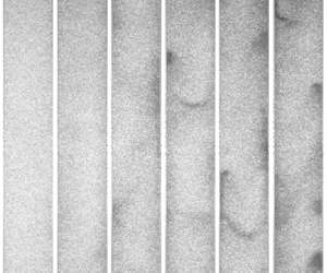
The above analysis indicates that, above a certain concentration, the sharp increase in fluctuations is associated with the appearance of mesoscale structures of relatively large density and fall speed. The appearance of such clusters with increasing  $\varPhi _V$ is evident from visual inspection, as illustrated in the instantaneous snapshots in figure 14. In this section, we describe a methodology to detect and track clusters, and characterise their properties. The analysis is carried out only for cases with $\varPhi _V \geq 5\times 10^{-3}$; more dilute cases (in which clusters are not visually identified) return noise-dominated results.
Sample instantaneous backlighting images from all considered cases, with volume fraction increasing from left to right.

4.1. Cluster detection and tracking
Several methodologies have been used in the past to detect clusters in gas–solid flows. Although the differences between setups and the various measurement and simulation techniques have prevented the definition of a universal criterion, many studies have applied definitions similar to those proposed by Soong, Tuzla & Chen (Reference Soong, Tuzla and Chen1993): (i) the cluster concentration must be significantly higher than the mean concentration; (ii) the cluster must be at least one or two orders of magnitude larger than an individual particle; and (iii) the cluster must exist for a time duration much longer than the minimum sampling time. Concerning criterion (i), in the literature the choice of the concentration threshold has varied widely, often being based on its mean and standard deviation (see Cahyadi et al. Reference Cahyadi, Anantharaman, Yang, Karri, Findlay, Cocco and Chew2017 and references therein); however, the meaning of the latter is questionable when the distribution is far from Gaussian, as in most gas–solid flows (Guenther & Breault Reference Guenther and Breault2007).
Here we utilise the percolation method, which has been widely used to identify coherent structures in single-phase turbulent flows (Moisy & Jiménez Reference Moisy and Jiménez2004; Del Alamo et al. Reference Del Alamo, Jimenez, Zandonade and Moser2006; Lozano-Durán, Flores & Jiménez Reference Lozano-Durán, Flores and Jiménez2012; Carter & Coletti Reference Carter and Coletti2018) and recently to characterise clusters of falling snowflakes in the atmosphere (Li et al. Reference Li, Lim, Berk, Abraham, Heisel, Guala, Coletti and Hong2021a). The concentration field  $C$ is binarised based on a threshold $C^*$, and the number of connected cells with $C > C^*$ are identified and counted for different values of the threshold. As $C^*$ increases the number of detected clusters grows, until these regions start to merge into a few large objects. The process is illustrated in figure 15(a), which highlights the chosen threshold corresponding to the maximum number of identified clusters (Lozano-Durán et al. Reference Lozano-Durán, Flores and Jiménez2012; Carter & Coletti Reference Carter and Coletti2018; Li et al. Reference Li, Lim, Berk, Abraham, Heisel, Guala, Coletti and Hong2021a). For a sample realisation, figure 15(b,c) show instantaneous concentration and velocity fields, respectively. The boundaries of the identified clusters are overlaid, with crosses indicating their centroids. A minimum size threshold of $2\times 2$ contiguous cells is applied, which effectively imposes a minimum length scale for the cluster of $\sim 10d_p$ (according to criterion (ii)).
(a) Number of detected clusters as function of concentration threshold in the percolation analysis, with the vertical dashed line indicating the selected threshold. (b) Sample concentration field for the case  $\varPhi _V =7.7\times 10^{-3}$, $Re_{bulk} = 1200$, with contour lines indicating cluster boundaries and crosses indicating their centroids. (c) Vertical velocity field for the realisation in (b), with the cluster boundaries again shown.

In addition, we leverage the time-resolved nature of the data to estimate the cluster lifetimes. The procedure is adapted from that developed by Liu et al. (Reference Liu, Shen, Zamansky and Coletti2020) for characterising the temporal evolution of inertial particle clusters in turbulence. The tracking is performed via a nearest-neighbour algorithm applied to the cluster centroids, the result of which is found to be relatively insensitive to the search radius (as long as the latter is of the order of the expected displacement based on the local mean velocity). When the tracking algorithm fails to find the successive centroid location within the search radius, three scenarios are contemplated: the cluster has either disintegrated into components below the concentration/size thresholds, merged with another cluster, or split into smaller clusters. To account for the second and third scenarios (which effectively extend the cluster lifetime), adjacent clusters are considered: if one of them overlaps with the former cluster over more than 50 % of its area, it is recognised as the same cluster and the tracking continues. A minimum lifetime threshold is then applied based on the expected time scale of random (Brownian) fluctuations in the concentration field, which is taken as the characteristic time between successive inter-particle collisions as described earlier in § 3.1. In the denser cases for which clusters are detected,  $n \sim 1.5$ mm $^{-3}$ and $t_{coll} \sim 10$ ms. This is much longer than the interval between successive images, according to criterion (iii).
4.2. Cluster characteristics for the denser case
In this section, we address the properties, position and velocity of clusters for the case at highest volume fraction ( $\varPhi _V =7.7\times 10^{-3}$, $Re_{bulk} = 1200$), based on the 1512 clusters detected and tracked during the recording time. The other dense cases display qualitatively similar trends.
The cluster area  $A_{cluster}$ (as captured by the two-dimensional projection) has a broad distribution shown in figure 16(a): the typical length scale is of the order of the duct half-width $h$, but approximately 20 % of the clusters have areas larger than the channel cross-section. The p.d.f. of the concentration $C_{cluster}$, obtained by averaging $C$ over all cells belonging to each cluster, exhibits a bimodal shape with a peak at relatively low concentrations (figure 16b). This corresponds to clusters of relatively small size found adjacent to the walls. This is illustrated in figure 17, which shows joint p.d.f.s of wall-normal centroid locations with $A_{cluster}$ and $C_{cluster}$, respectively. The clusters are commonly located near the walls, in line with visual observations and previous experiments (Cahyadi et al. Reference Cahyadi, Anantharaman, Yang, Karri, Findlay, Cocco and Chew2017). Their concentration and size increases with the wall-normal distance up to approximately $0.3h$. As the cluster location is defined by its centroid, the increase in size with wall distance may be simply the result of larger clusters having larger wall-normal extension.
Probability distributions of (a) projected cluster area and (b) in-cluster concentration for the case  $\varPhi _V =7.7\times 10^{-3}, Re_{bulk} = 1200$.

Joint p.d.f.s of (a) cluster area and centroid wall-normal location and (b) in-cluster concentration and centroid wall-normal location, for the case  $\varPhi _V =7.7\times 10^{-3}$, $Re_{bulk} = 1200$.

The correlation between  $A_{cluster}$ and $C_{cluster}$, which can be deduced from figure 17, is demonstrated in the scatter plot of both variables in figure 18(a): a linear regression indicates that the concentration in a cluster grows approximately as the square root of its area. The values are averaged over each cluster lifetime, which is also indicated by the colour-coding of the data points; this indicates that larger and denser clusters also have longer lifetimes. Figure 18(b) presents the joint p.d.f. of cluster concentration $C_{cluster}$ and vertical velocity $U_{cluster}$. The latter is defined as the velocity of the cluster centroid; other definitions (e.g. averaging $U$ over all cluster cells) yield similar results. Despite large scatter (which can be attributed to the broad range of the object sizes and shapes, as well as to the variance of the observables within each cluster), it is clear that denser clusters tend to fall faster. This is consistent with observations from two-fluid (Agrawal et al. Reference Agrawal, Loezos, Syamlal and Sundaresan2001) and Euler–Lagrange (Capecelatro et al. Reference Capecelatro, Pepiot and Desjardins2014; Capecelatro & Desjardins Reference Capecelatro and Desjardins2015) simulations in confined and periodic geometries. Taken together, these results indicate that larger clusters are denser and longer-lived, and also have a larger descent velocity.
(a) Scatter plot of the in-cluster concentration versus cluster area. Both variables are averaged over a cluster lifetime, which is normalised by  $\tau _p$ and used to colour-code each data point. (b) Joint p.d.f. of the cluster descent velocity against the cluster concentration , displaying a weak positive correlation ( $\textrm {slope} = 0.34$, $r^2 = 0.06$) between both variables. Both panels are for the case $\varPhi _V =7.7\times 10^{-3}$, $Re_{bulk} = 1200$.

4.3. Comparison among the denser cases
In order to evaluate the effect of varying parameters, the size, shape, position and velocity of the clusters are evaluated for the four denser cases. For these cases, an increase in  $Re_{bulk}$ is associated with an increase in $\varPhi _V$, thus the effect of both parameters cannot be disentangled. Although $\varPhi _V$ has been shown to be the controlling parameter across the parameter space, the four-fold change in air flow rate across these four cases is likely to be at least as consequential as the $\sim 50$ % change in volume fraction.
Figure 19(a) displays p.d.f.s of  $A_{cluster}$, indicating that the size distribution becomes wider, and its mean becomes smaller with increasing $Re_{bulk}$. The broader size distribution is expected as the system displays larger fluctuations, whereas the smaller size is likely associated with more frequent breakup events, consistent with the fact that smaller clusters have shorter lifetimes. The clusters are observed to be vertically elongated, which can be quantified in terms of geometric aspect ratio. To this end, we use a singular value decomposition approach similar to Baker et al. (Reference Baker, Frankel, Mani and Coletti2017), calculating the cluster spread along its larger ( $s_1$) and smaller ( $s_2$) principal axes. The aspect ratio $s_2/s_1$ has limit values of 0 for an infinitely thin elongated object and 1 for a square or circular one. The p.d.f. of aspect ratios indicate highly elongated clusters, especially for lower $Re_{bulk}$ (figure 19b). Considering that most clusters are vertically oriented, typical values of the aspect ratio ( $s_2/s_1 \sim 0.1$) and area ( $A_{cluster} \sim h^2$) indicate that their vertical extent is ${\sim }3 - 4h$. This is roughly consistent with the size of the correlation length in figure 9.
Comparison between the four cases where clusters are observed. (a) Probability distributions of projected cluster area. (b) Probability distributions of cluster aspect ratio. (c) Profiles of the number of detected clusters at each wall-normal location ( $N_{clusters}$) normalised by the total number of detected clusters ( $N_{all}$). (d) Profiles of the mean cluster descent velocity. (e) Probability distributions of the cluster descent velocity. (f) Probability distribution of the cluster descent velocity relative to the bulk velocity of the upward moving air $U_{bulk}$.

For all cases, the cluster centroids are found in the vicinity of the wall, a tendency more marked for lower  $Re_{bulk}$ (figure 19c). In previous studies of dense riser configurations, it is often assumed that the proximity to the wall puts the clusters in the boundary layer of the rising fluid, allowing their relatively fast descent (Noymer & Glicksman Reference Noymer and Glicksman2000). Figure 19(d), however, indicates that $U_{cluster}$ near the walls is not systematically larger than in the core of the duct. For $Re_{bulk} = 300$ and 600, the main trend is the asymmetry of the profiles (also seen in the mean particle velocity $\langle U \rangle$, see figure 5), while for the denser cases the descent velocity is approximately homogeneous. In contrast, $\langle U \rangle$ for $Re_{bulk} = 900$ and 1200 near the wall is approximately twice as high as at the centre-plane (see figure 5). One should consider, however, that the cluster statistics away from the wall are affected by larger uncertainties due to the much fewer samples. The distribution of $U_{cluster}$ becomes broader with increasing $Re_{bulk}$ and its mean is consistently larger than $\langle U \rangle$ (figure 19e). Overall, the cluster velocity display qualitatively similar features as the convection velocity from the autocorrelation maps: it is larger than the mean vertical velocity and does not strongly depend on the wall-normal location. The mean cluster fall speed is smaller than the convection velocity deduced from the $R_{cc}$ map (figure 9d–f), which is the characteristic velocity of coherent structures in the concentration field. This is likely because the denser clusters, which fall faster than the mean of $U_{cluster}$, leave a stronger footprint on the concentration autocorrelation.
Finally, we note that the cluster descent velocity relative to the bulk velocity of the upward moving fluid,  $U_{cluster} - U_{bulk}$, is of the order of the particle terminal velocity $U_t$ for all cases (figure 19f). The latter is quantitatively close to the semi-empirical expression of the descent velocity proposed by Noymer & Glicksman (Reference Noymer and Glicksman2000) for near-wall clusters in circulating fluidised beds, $U_{NG} = 0.75\sqrt {g d_p (\rho _p/\rho _f )}$ $(U_{NG} = 1.56$ m s $^{-1}$ in this experiment, which is close to $U_t$). This assumes no influence of the fluid velocity and was found to agree reasonably well with laboratory observations and numerical simulations (Capecelatro et al. Reference Capecelatro, Pepiot and Desjardins2014). In our case, on the other hand, this prediction is only tenable if $U_{NG}$ is interpreted as a descent velocity relative to the fluid. Importantly, compared with the cases considered by Noymer & Glicksman (Reference Noymer and Glicksman2000), the present experiments are conducted at significantly lower volume fraction, and a strong influence of the fluid velocity is expected.
5. Conclusions
We have reported on a series of experiments conducted in a riser-type apparatus where spherical particles fall in a duct against upward moving air: a typical configuration in industrial gas–solid flows. Unlike previous studies, we vary independently the particle volume fraction  $\varPhi _V$ and the air flow Reynolds number $Re_{bulk}$. Using a backlighting approach, we evaluate the spatiotemporal evolution of the particle concentration and velocity fields. The upward air flow slows the particle descent by a magnitude comparable to $U_{bulk}$, implying that the particle slip with respect to the flow is of the order of the still-air terminal velocity of an isolated particle $U_t = g\tau _p$. The dynamics, however, is far more complex than what suggested by such a simple scaling. For the most dilute cases, the system is approximately homogeneous and displays small uncorrelated fluctuations. Above a critical threshold $\varPhi _V \sim 5\times 10^{-3}$ (which appears largely independent of $Re_{bulk}$) the fluctuations of velocity and concentration increase sharply as mesoscale clusters are formed. This is consistent with recent observations by Weit et al. (Reference Weit, Roche, Dubois and Manga2018), who reported the formation of clusters of fluidised particles in a vertical pipe above a critical volume fraction of $\varPhi _V \sim 0.01$. Although the origin of the fluctuating energy is in the particle–fluid slip rather than in the mean shear, the fluctuation covariances do vary approximately linearly with the spatial gradients, supporting the use of the gradient-diffusion assumption. The space–time autocorrelations indicate the presence of dense and persistent structures with typical vertical lengths of the order of the channel width, falling faster than the average particles and trailing long wakes. These are shown to be the statistical footprints of the visually observed clusters, which are identified via a percolation analysis, tracked in time, and characterised in terms of size, shape, location and descent velocity. The clusters are highly elongated in the vertical direction, often longer than the channel width, are found mostly in the vicinity of the wall, and fall faster than the surrounding dilute particles. Larger clusters are denser and longer-lived and have larger descent velocity. The latter is weakly dependent on the distance from the wall.
The parameter space deserves emphasis. The volume fraction lies in a range ( $\varPhi _V = 10^{-3} - 10^{-2}$) which is rarely investigated in systematic gas–solid flow experiments, despite its relevance not only to industrial applications such as pneumatic transport (Louge, Mastorakos & Jenkins Reference Louge, Mastorakos and Jenkins1991) but also to geophysical phenomena such as snow avalanches (Sovilla, McElwaine & Louge Reference Sovilla, McElwaine and Louge2015) and pyroclastic currents (Dufek Reference Dufek2016). This is, in fact, a regime for which data are sorely needed, as it challenges existing numerical models: the concentration is too dense for approaches where collisions are neglected (Kasbaoui et al. Reference Kasbaoui, Koch and Desjardins2019), but too dilute for the collisional state to reach statistical equilibrium (Fox Reference Fox2014). Even for the denser cases we considered, the expected mean free path $\lambda$ ranges between 5 and 7 mm, and thus the Knudsen number (the ratio between the mean free path and the length scale over which the spatial gradients are expressed) $Kn = \lambda /h =$ $O(1)$, violating the low- $Kn$ assumption in kinetic-theory-based models (Garzó et al. Reference Garzó, Tenneti, Subramaniam and Hrenya2012).
The range of  $Re_{bulk} \leq 1200$ would imply a fully laminar single-phase flow, whereas a sufficient number of particles induces a highly unsteady-state characterised by large multiscale fluctuations of concentration and velocity. Although the air velocity fields cannot be explored here, this regime bears the hallmarks of cluster-induced turbulence (Capecelatro & Desjardins Reference Capecelatro and Desjardins2015): when gravity acts on particle-laden flows with $\varPhi _V \ll 1$ and $\varPhi _M > 1$, clusters form and entrain fluid, falling at relatively large speed and generating strong velocity gradients, which, in turn, feed high fluctuating energy that exhibits large correlation lengths. The latter scales with $g\tau _p^2$ in homogeneous systems, but in internal flows the cluster size is limited by the duct diameter (Capecelatro, Desjardins & Fox Reference Capecelatro, Desjardins and Fox2016). Although visual evidence of clusters in these regimes has been reported previously (Weit et al. Reference Weit, Roche, Dubois and Manga2018), this is the first documentation of their footprint on the spatiotemporal velocity of the particle fields, and thus represents a first experimental observation of cluster-induced turbulence.
These results can be interpreted in light of the clustering mechanisms proposed in previous theoretical and numerical studies. First, the fact that the fluctuations of particle velocity and concentration are convected at different speeds supports classic arguments on the system instability (Fullmer & Hrenya Reference Fullmer and Hrenya2017). Moreover, the relation between velocity and concentration agrees with the notion that clusters experience a concentration-dependent drag: larger clusters fall faster and grow by incorporating particles they meet in their descent (Capecelatro & Desjardins Reference Capecelatro and Desjardins2015). Finally, the threshold beyond which clustering ensues may be interpreted as the condition for which particles have insufficient time to respond to the fluid drag before the next collision, i.e.  $t_{coll} < \tau _p$. Estimates of $t_{coll}$ and theoretical arguments derived for homogeneous systems suggest a critical volume fraction remarkably close to the observed one, $\varPhi _V = 5\times 10^{-3}$. However, the presence of the walls is expected to affect the inception of clustering due to both local shear and inelastic particle-wall collisions. To verify that clustering for this class of gas–solid flows occurs beyond a critical volume fraction, and to ascertain the role of the particle response time in setting this value, further studies comparing different particle sizes and materials are warranted.
The present imaging approach relies on the optical depth-averaging of the fields in the  $z$ direction. Although the assumed averaging is consistent with zoomed-in measurements at the channel centre-plane (see the Appendix), it is likely that the quantitative values of local volume fraction are affected by inaccuracies in the intensity/concentration relation, especially within the clusters where the light attenuation is stronger than in the free-fall calibration experiments. However, this is not expected to overshadow the important trends which rely on relative concentration. The depth-averaging itself will blur the fine-scale features of the fields, especially when multiple small structures are in the line of sight. The fact that the denser clusters (which leave the stronger signature on the statistics) have sizes of the order of the channel width suggests that the macroscopic features of the system are captured. Still, future measurements are needed to address two main outstanding aspects which are outside the scope of the present study. First, the particle-scale dynamics shall be characterised by tracking individual particles. This will be challenging over the present range of concentrations unless intrusive probes are used, but would be essential to disentangle open questions; among others, whether the observed behaviour is mainly driven by collisions or by concentration-dependent drag. Second, volumetric imaging has greatly progressed in recent years, as mentioned in the introduction, and can be used to address the three-dimensional structure of the fields. Finally, we remark that the present configuration and regime lends itself well to numerical validation: in a 20 $h$ long section of the duct at the highest considered concentration, the total number of particles is $\sim 10^5$, which is within reach of the most advanced massively parallel PR-DNS approaches (Horne & Mahesh Reference Horne and Mahesh2019).
Declaration of interest
The authors report no conflict of interest.
Funding
This work was supported by the National Science Foundation (grant CBET-1903564).
Appendix. Enlarged-view imaging along the centre-plane
These measurements are only conducted for the more dilute regimes,  $\varPhi _V < 3 \times 10^{-3}$, as denser concentrations would impede the identification of individual particles. The backlighting imaging system described in § 2.2 is used with a different optical setting: a 200 mm Nikkor lens is mounted with aperture $f/4$, yielding a thin depth of focus in the $z$ direction and a field of view of 30.6 mm (or approximately $3h$) in the $x$ direction. This allows imaging around the $z/h =$1 plane (figure 20), with the focal plane position determined by traversing a calibration target on a micro-metric stand inserted in the duct. The resolution of 31.3 pixels per millimetre allows individual particles to be resolved and tracked. The internal diffraction from the glass spheres result in a ring-shaped pattern which requires a specialised procedure to locate the particle centroid, as illustrated in figure 21.
(i) The images are inverted and background subtraction is performed using the minimum intensity over the 20 000 image set.
(ii) The gradient of the background-subtracted image is computed, further sharpening the pattern of the in-focus particles.
(iii) The gradient image of an in-focus particle is cross-correlated across the gradient image to obtain a correlation map, and peak-finder algorithm is applied to find local maxima. The procedure is virtually insensitive to the choice of the in-focus particle.
(iv) To obtain sub-pixel accuracy on the particle centroid location, a 3-point Gaussian fit is applied to the correlation map around the local maxima.
(a) Imaging setup for the enlarged-view measurements. (b) Sample image obtained with this approach for the case  $\varPhi _V =1.0\times 10^{-3}$, $Re_{bulk} = 300$.

A sequence of images illustrating the particle identification procedure: (a) inverted particle image; (b) corresponding gradient image sharpening the in-focus particles; (c) correlation map obtained by cross-correlating (b) with the gradient image of an in-focus particle, with local maxima marked by blue crosses; (d) close-up view showing the peak-locked centroid (blue cross) and the sub-pixel accurate centroid (red dot) for the particle shown in the red box in (c).

The acquisition frequency is at 4300 Hz, resulting in inter-frame particle displacement between 2 and 9 pixels (or approximately  $0.3 - 1.4$ particle image diameters). Particle motion is reconstructed using an in-house PTV algorithm described in Petersen, Baker & Coletti (Reference Petersen, Baker and Coletti2019) and Baker & Coletti (Reference Baker and Coletti2021), returning Lagrangian trajectories and the associated velocities and accelerations. To produce Eulerian fields comparable to the zoomed-out measurements, the Lagrangian PTV data is binned spatially on a grid congruent to the PIV interrogation windows). In order to quantify the mean concentration, the in-focus particles are counted within the imaging volume. The depth of the latter is determined by traversing on the micrometric stand a pair of transparent slides sandwiching sparse glass particles. Figure 22 shows the number of in-focus particle detected as the slide is moved in the $z$ direction, from which depth-of-focus is determined to be 2 mm.
Plot of number of particles detected on the microscopic glass slide against the slide position.


 Open access