


1. Introduction
Particle-laden flow in horizontal rotating cylinders is encountered in several applications, including coating processes, pharmaceutical industries, paste preparation for composite membranes, microbiological cultures, etc. This has been of interest to physicists owing to the several non-equilibrium phases exhibited by such systems besides the intriguing phenomenon of axial pattern formation. It is well known that heterogeneous mixtures of dry granular materials segregate under various flow conditions such as vibration, shaking, rotation and mechanical agitation (Ottino & Khakhar Reference Ottino and Khakhar2000). When a horizontal cylinder partially filled with a heterogeneous mixture of dry grains is rotated, the grains segregate by size and/or density to form axial patterns (Seiden, Lipson & Franklin Reference Seiden, Lipson and Franklin2004). The dynamic angle of repose is considered to be the control parameter for axial pattern formation for dry heterogeneous granular mixtures (Inagaki & Yoshikawa Reference Inagaki and Yoshikawa2010). It is noted that the end walls of the rotating drum initiate axial band formation via an axial flow due to friction at the end walls (Chen, Ottino & Lueptow Reference Chen, Ottino and Lueptow2010; Arntz et al. Reference Arntz, den Otter, Beeftink, Boom and Briels2013; Jain, Fabien & van Wachem Reference Jain, Fabien and van Wachem2023).
A rotating suspension of neutrally buoyant particles partially filling a rotating cylinder also displays axial pattern formation even with monodispersed particles (Tirumkudulu, Tripathi & Acrivos Reference Tirumkudulu, Tripathi and Acrivos1999; Tirumkudulu, Mileo & Acrivos Reference Tirumkudulu, Mileo and Acrivos2000; Thomas et al. Reference Thomas, Riddell, Kooner and King2001; Timberlake & Morris Reference Timberlake and Morris2002). For such cases of the rimming flow of suspensions, it has been proposed that the differential drainage of the particle and the fluid phases drives axial segregation (Timberlake & Morris Reference Timberlake and Morris2003).
In addition, a non-neutrally buoyant dilute suspension, entirely filling a horizontal rotating cylinder, experiences axial segregation (Breu, Kruelle & Rehberg Reference Breu, Kruelle and Rehberg2004; Seiden, Ungarish & Lipson Reference Seiden, Ungarish and Lipson2005; Kalyankar et al. Reference Kalyankar, Matson, Tong and Ackerson2008). For dilute suspensions (volume fraction  $\phi \sim 0.02$), axial variations in particle concentration are amplified by a buckling instability driving high-density regions to fall faster, subsequently drawing more particles into this region (Lee & Ladd Reference Lee and Ladd2005). Experimental (Kumar & Singh Reference Kumar and Singh2010; Nasaba & Singh Reference Nasaba and Singh2018, Reference Nasaba and Singh2020) and theoretical (Hou, Pan & Glowinski Reference Hou, Pan and Glowinski2014; Lopes, Thiele & Hazel Reference Lopes, Thiele and Hazel2018; Konidena, Reddy & Singh Reference Konidena, Reddy and Singh2019) studies indicate that the interplay between centrifugal, gravitational and drag forces causes axial bands for the dilute suspension system. However, a unifying mechanism to explain the axial pattern formation phenomenon is still lacking. The behaviour of a dense suspension in a rotating cylinder, alongside the influence of end walls, is also unexamined in previous works (Seiden et al. Reference Seiden, Lipson and Franklin2004). It should be emphasized that the axial banding phenomenon is not exhibited with a neutrally buoyant particle suspension fully filling a rotating cylinder; interplay between the centrifugal force, drag and gravitational force is very much essential for the axial banding phenomenon (Kalyankar et al. Reference Kalyankar, Matson, Tong and Ackerson2008; Konidena et al. Reference Konidena, Lee, Reddy and Singh2018).
Understanding the mechanism of axial band formation is significant as it elucidates the (de)mixing behaviour exhibited by the viscous dense suspension. It is well known that the steady-state rheology of a non-Newtonian fluid is governed by the three degrees of freedom of the stress tensor, i.e. the viscosity ( $\eta _{s}$) and two normal stress differences ( $N_1$ and $N_2$). In concentrated suspensions, e.g. $\phi > 0.22$ (Guazzelli & Pouliquen Reference Guazzelli and Pouliquen2018), the anisotropy of the microstructure results in the particle normal stresses which drive migration (Morris & Boulay Reference Morris and Boulay1999; Sierou & Brady Reference Sierou and Brady2002). The previous works to explore the influence of $N_1$, $N_2$ and shear-induced migration for gravity-driven particle-laden flows are sparse (Dhas & Roy Reference Dhas and Roy2022) and have not investigated axial patterns in rotating flows.
In this work, we perform numerical simulations by varying the three degrees of freedom of the stress tensor. The effect of the presence of cylinder end walls is also examined. We report a non-periodic axial band pattern in a rotating dense suspension resembling the discontinuous banding phase exhibited by viscous suspensions (Kalyankar et al. Reference Kalyankar, Matson, Tong and Ackerson2008; Matson, Ackerson & Tong Reference Matson, Ackerson and Tong2008). As a significant result, we propose a mechanism for the axial pattern formation in a dense suspension, fully filling a horizontal rotating cylinder. The first two terms of the shear viscosity ( $\eta _{s}$ taken from Boyer, Guazzelli & Pouliquen Reference Boyer, Guazzelli and Pouliquen2011) initiate an instability along the axial plane; this instability becomes accentuated by the influence of stress anisotropy. The third term of the shear viscosity ( $\eta _s$ given by (2.12)) $(1-\phi /\phi _m)^{-2}$, negates the action of $N_2$ and pushes the particle phase towards the end walls. This eventually leads to the formation of a non-uniformly distributed pattern along the axis of rotation.
2. Mathematical model and simulation set-up
To model the concentrated suspension of non-Brownian particles, we use the original version of the suspension balance model (SBM) (Nott & Brady Reference Nott and Brady1994; Morris & Boulay Reference Morris and Boulay1999), which ascribes particle migration to gradients in the particle stress tensor  $\boldsymbol {\varSigma }_{p}$ (Ramachandran & Leighton Reference Ramachandran and Leighton2008). In the model described below, the particle stresses and the contact stresses are identical, unlike in a more generic SBM, which is a diphasic model (which has more than three degrees of freedom identified at the macroscopic level) (Lhuillier Reference Lhuillier2009; Nott, Guazzelli & Pouliquen Reference Nott, Guazzelli and Pouliquen2011). The SBM applies the principles of conservation of mass and momentum for the fluid and particle phases. For the bulk suspension, the particle size is sufficiently large to bypass the effects of Brownian motion, and the fluid is sufficiently viscous to neglect inertia. Therefore, the steady-state mass and momentum balance equations for the conditions described are written as
 $$\begin{gather} \boldsymbol{\nabla}\boldsymbol{\cdot}\boldsymbol{u} = 0, \end{gather}$$
 $$\begin{gather}\boldsymbol{\nabla}\boldsymbol{\cdot}\boldsymbol{\varSigma} + \rho \boldsymbol{g} = 0, \end{gather}$$
where  $\boldsymbol {u}$ is the velocity of the bulk suspension, $\boldsymbol {g}$ is gravity and $\boldsymbol {\varSigma }$ is the bulk suspension stress (which will be shown later in (2.7)). Using the particle volume fraction $\phi$, the total mixture density $\rho$ is given by
 \begin{equation} \rho = \phi \rho_{p} + (1 - \phi) \rho_{f}, \end{equation}
where  $\rho _{p}$ and $\rho _{f}$ are the densities of the particle and the fluid phases, respectively. Thus, (2.2) can be rewritten as
 \begin{equation} \boldsymbol{\nabla}\boldsymbol{\cdot}\boldsymbol{\varSigma} + \Delta \rho \phi \boldsymbol{g} = 0, \end{equation}
where  $\Delta \rho \equiv \rho _{p} - \rho _{f}$. Note that the constant body force $\rho _{f} \boldsymbol {g}$ is omitted in (2.4).
The continuity and momentum equations ((2.1) and (2.4)) are solved in tandem with the particle-phase conservation equation given as
 \begin{equation} \frac{\partial \phi}{\partial t} + \boldsymbol{u}\boldsymbol{\cdot}\boldsymbol{\nabla} \phi ={-} \boldsymbol{\nabla}\boldsymbol{\cdot}{\boldsymbol{j}}_{t}, \end{equation}
with  $\boldsymbol {j}_{t}$ being the total migration flux. Here, $\boldsymbol {j}_{t}$ is written as a sum of the particle migration flux due to the cross-streamline migration $\boldsymbol {j}_{\perp }$ and the additional flux term due to the effect of a non-neutrally buoyant particle phase $\boldsymbol {j}_{g}$
 \begin{equation} \boldsymbol{j}_{t} =
\underbrace{\frac {2a^2}{9 \eta_0} f(\phi)[\boldsymbol{\nabla}\boldsymbol{\cdot} \boldsymbol{\varSigma}^p]}_{\boldsymbol{j}_{{\perp}}}+
\underbrace{\frac{2a^2}{9 \eta_0} f(\phi) [\Delta \rho \phi\boldsymbol{g} ]}_{\boldsymbol{j}_{g}}. \end{equation}
\begin{equation} \boldsymbol{j}_{t} =
\underbrace{\frac {2a^2}{9 \eta_0} f(\phi)[\boldsymbol{\nabla}\boldsymbol{\cdot} \boldsymbol{\varSigma}^p]}_{\boldsymbol{j}_{{\perp}}}+
\underbrace{\frac{2a^2}{9 \eta_0} f(\phi) [\Delta \rho \phi\boldsymbol{g} ]}_{\boldsymbol{j}_{g}}. \end{equation} In (2.6),  $a$ is the suspended particle radius and $\eta _0$ is the fluid viscosity. The parameter $f(\phi )$ is the sedimentation hindrance function, which indicates the mobility of the particle phase; its form $f(\phi ) = (1-\phi /\phi _{m}) (1 - \phi )^{\alpha - 1}$ as used in this work is given by Richardson & Zaki (Reference Richardson and Zaki1954). The parameter $\alpha$ is taken as 2 and the maximum volume fraction of the solid phase $\phi _{m}$ is $0.58$ (Miller, Singh & Morris Reference Miller, Singh and Morris2009) for the simulations in this work. Since the time evolution of migration is sufficiently slow (Breu et al. Reference Breu, Kruelle and Rehberg2004; Kalyankar et al. Reference Kalyankar, Matson, Tong and Ackerson2008; Matson et al. Reference Matson, Ackerson and Tong2008), the reported states are always near steady state
 \begin{equation} \boldsymbol{\varSigma} ={-}p \boldsymbol{\mathsf{I}} + 2\eta_0\eta_{s} \boldsymbol{\mathsf{D}} + 2\zeta_{0} \boldsymbol{\mathsf{E}} + 2\zeta_{3} \boldsymbol{\mathsf{G}}_3. \end{equation}
The bulk suspension stress tensor equation (2.7) is essentially decomposed in terms of its components on a tensorial basis adapted to local flow conditions. This tensorial basis is determined solely by the symmetric part of the velocity gradient,  $\boldsymbol{\mathsf{D}}$ as in Giusteri & Seto (Reference Giusteri and Seto2018). Particle stress is calculated as $\boldsymbol {\varSigma }_{p} = \boldsymbol {\varSigma } - \boldsymbol {\varSigma }_{f}$ from the knowledge of $\boldsymbol {\varSigma }_{f} = -p_{f} \boldsymbol{\mathsf{I}} + 2\eta _0 \boldsymbol{\mathsf{D}}$. In (2.7), the terms $\boldsymbol{\mathsf{D}}$, $\boldsymbol{\mathsf{E}}$ and $\boldsymbol{\mathsf{G}}_3$ for planar flows are defined in Giusteri & Seto (Reference Giusteri and Seto2018) as $\boldsymbol{\mathsf{D}} = ({\dot {\gamma }}/{2}) [ \widehat {\boldsymbol {d}_1} \widehat {\boldsymbol {d}_1} - \widehat {\boldsymbol {d}_2}\widehat {\boldsymbol {d}_2} ]$, $\boldsymbol{\mathsf{E}} = ({\dot {\gamma }}/{4}) [ -\widehat {\boldsymbol {d}_1} \widehat {\boldsymbol {d}_1} - \widehat {\boldsymbol {d}_2}\widehat {\boldsymbol {d}_2} + 2\widehat {\boldsymbol {d}_3}\widehat {\boldsymbol {d}_3} ]$ and $\boldsymbol{\mathsf{G}}_{3} = ({\dot {\gamma }}/{2})(\widehat {\boldsymbol {d}_2}\widehat {\boldsymbol {d}_1} + \widehat {\boldsymbol {d}_1}\widehat {\boldsymbol {d}_2})$. Here, $\widehat {\boldsymbol {d}_1}$, $\widehat {\boldsymbol {d}_2}$ and $\widehat {\boldsymbol {d}_3}$ are orthonormal eigenvectors of $\boldsymbol{\mathsf{D}}$. The parametric tensor $\boldsymbol{\mathsf{Q}}$ which captures the anisotropy of the particles in Miller et al. (Reference Miller, Singh and Morris2009) is also enveloped in (2.7). The response coefficients $\zeta _0$ and $\zeta _3$ are related to $\lambda _2$ and $\lambda _3$ of the parametric tensor $\boldsymbol{\mathsf{Q}}$ in Miller et al. (Reference Miller, Singh and Morris2009) as
 $$\begin{gather} \zeta_0 = \frac{\eta_0 \eta_{n} }{3} (1+\lambda_2 - 2\lambda_3), \end{gather}$$
 $$\begin{gather}\zeta_3 = \frac{\eta_0 \eta_{n}}{2} (1-\lambda_2). \end{gather}$$
We recall that, for simple shear, one finds (Giusteri & Seto Reference Giusteri and Seto2018)
 $$\begin{gather} N_1 ={-}2\dot{\gamma}\zeta_3, \end{gather}$$
 $$\begin{gather}N_2 = \dot{\gamma}\zeta_3 - \tfrac{3}{2}\dot{\gamma}\zeta_0. \end{gather}$$
Equations (2.10) and (2.11) provide a relation between the first and the second normal stress differences ( $N_1$ and $N_2$, respectively) and the response coefficients ( $\zeta _3$ and $\zeta _0$) of the constitutive relation for the bulk stress equation (2.7). The shear and normal viscosities (made dimensionless by taking the ratio with fluid viscosity $\eta _0$) are as given by Morris & Boulay (Reference Morris and Boulay1999) and Boyer et al. (Reference Boyer, Guazzelli and Pouliquen2011)
 $$\begin{gather} \eta_{s} (\phi) =
\underbrace{1 + 2.5 \phi \left(1-\dfrac{\phi}{\phi_{m}} \right)^{{-}1}}_{\eta_{{s1}}(\phi)} +
\underbrace{\mu^c (\phi) \left(\dfrac{\phi}{\phi_{m} - \phi}\right)^2}_{\eta_{{s2}} (\phi)}, \end{gather}$$
$$\begin{gather} \eta_{s} (\phi) =
\underbrace{1 + 2.5 \phi \left(1-\dfrac{\phi}{\phi_{m}} \right)^{{-}1}}_{\eta_{{s1}}(\phi)} +
\underbrace{\mu^c (\phi) \left(\dfrac{\phi}{\phi_{m} - \phi}\right)^2}_{\eta_{{s2}} (\phi)}, \end{gather}$$ $$\begin{gather}\eta_{n} (\phi)= \left(\frac{\phi}{ \phi_{m} - \phi}\right)^2, \end{gather}$$
where  $\mu ^{c} (\phi ) = \mu _1 + (\mu _2 - \mu _1)/[1+ I_0 \eta _{n} (\phi )]$. In Boyer et al. (Reference Boyer, Guazzelli and Pouliquen2011), it has been shown that the frictional formalism of dense suspensions can be related to their classical viscous rheology. We implement the $\phi$-dependent friction law of dense suspensions proposed by Boyer et al. (Reference Boyer, Guazzelli and Pouliquen2011) as given by (2.12). The first two terms in (2.12) are denoted as $\eta _{{s1}} (\phi )$, and the third term is denoted as $\eta _{{s2}} (\phi )$.
The simulation parameters are close to the experimental works by Kumar & Singh (Reference Kumar and Singh2010), Kalyankar et al. (Reference Kalyankar, Matson, Tong and Ackerson2008) and Matson et al. (Reference Matson, Ackerson and Tong2008). The length of the cylinder  $L={0.2275}\ {\rm m}$ and the diameter is $D={0.02}\ {\rm m}$. The average particle concentration over the surface of the cylinder is $\phi _{avg}$. The size of an individual particle $D_{p}=2a$, which collectively comprises the particle phase, is ${200}\ {\mathrm {\mu }}{\rm m}$, and its density $\rho _{p} = {1000}\ {\rm kg}\ {\rm m}^{-3}$. The suspending liquid has a density $\rho _{f}={1200}\ {\rm kg}\ {\rm m}^{-3}$ with a viscosity of $\eta _0 = {0.055}\ {\rm Pa}\ {\rm s}$. The cylinder is rotated at a rotational velocity of $\varOmega = {5}\ {\rm rad}\ {\rm s}^{-1}$ and the particle velocity can be calculated using $u_{p} = 2a^2 g \Delta \rho / 9\eta _0$, which is ${0.0008}\ {\rm m}\ {\rm s}^{-1}$. The particle Reynolds number $Re_{p} = \rho _{p} D_{p} u_{p} / \eta _0$ is $0.0003$. At time
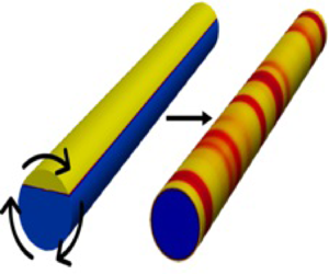
  $t=0$, the suspension configuration is as shown in figure 1(a), since the particles are buoyant, the concentration is higher at the top as indicated by the red colour ( $\phi =0.45$), and the blue colour indicates a concentration of $\phi =0.3$. The values of $\zeta _0= 0.233 \eta _{{0}} \eta _{n}$ and $\zeta _3= 0.1 \eta _0 \eta _{n}$ are used for the simulations, which are consistent with a concentrated suspension rheology (Miller et al. Reference Miller, Singh and Morris2009; Xiong et al. Reference Xiong, Angerman, Ellero, Sandnes and Seto2024). The contact contribution is chosen similar to dry granular media $(\mu _2=0.7$, $\mu _1=0.32$ and $I=0.005$) (Boyer et al. Reference Boyer, Guazzelli and Pouliquen2011).
(a) Suspension concentration at  $t=0$ (concentration in the blue region is $\phi = 0.3$, dark red colour region $x \geqslant L/2$ has $\phi = 0.4625$ and light red region $x < L/2$ has $\phi = 0.4375$) and mesh along the axis of rotation. The average concentration $\phi _{avg} = 0.35$. (b) Radial view of the discretized geometry by structured mesh.

3. Numerical implementation and validation
For the numerical implementation of the mathematical model detailed above, the mass, momentum and particle-phase conservation equations were solved with the open-source software OpenFOAM (Weller et al. Reference Weller, Tabor, Jasak and Fureby1998), which uses the finite volume method to solve the system of partial differential equations. To provide an initial instability in the concentration of the suspension along the axial plane, the concentration on the right half of the cylinder ( $x > L/2$) is $\phi = 0.4625$, and on the left half of the cylinder ( $x < L/2$) is $\phi = 0.4375$. The system of equations (2.1)–(2.5) is implemented by modifying the pimpleFoam solver to a custom solver which represents the SBM. More precisely, the PIMPLE (a combination of the Pressure implicit with splitting of operators method and Semi-Implicit Method for Pressure-Linked Equations) algorithm is implemented to iteratively solve (2.1) and (2.4), which describe the flow behaviour. Additionally, the transport equation (2.5) uses the Crank–Nicholson scheme in the discretization of $\partial \phi / \partial t$. Adjustable time stepping is done for simulations in this work, with the maximum allowable time step being restricted to $0.1$. A rotating wall boundary condition is imposed on the wall of the cylinder with no slip. A zero flux condition is applied on the walls and surface of the cylinder for the suspension concentration.
The mesh is generated using the blockMesh facility in OpenFOAM, with a total of 189 600 hexahedral cells. Grid independence studies were performed by comparing the concentration variation across the axial length of the cylinder for three different grid sizes. The first grid has a size of 120 000 with 600 cells in the axial direction and 200 cells in the radial direction (grid-A), the second grid has a total of 189 600 with 150 cells in the axial direction and 1264 cells in the radial direction (grid-B) and the third grid studied has 240 000 cells with 150 in the axial and 1600 in the radial directions (grid-C). The concentration profiles of the suspension for the three grid sizes investigated are shown in figure 2; very good agreement on the overlap of profiles indicates that the grid size has no influence on the concentration in the axial direction. For the simulations of a suspension rotating in a horizontal cylinder, we have used grid-B (189 600 cells).
Grid independence studies on the rotating geometry for three different grids: grid-A with 120 000 cells, grid-B with 189 600 cells and grid-C with 240 000 cells. The concentration profiles show excellent overlap and negligible variation with different grids.

In order to validate our mathematical model, we compared the concentration and velocity distributions in figures 3 and 4 for the flow of a non-neutrally buoyant suspension in a circular pipe with the MRI (magnetic resonance imaging) measurements by Altobelli, Givler & Fukushima (Reference Altobelli, Givler and Fukushima1991) and the numerical simulations (anisotropic and isotropic models) as discussed by Ramachandran & Leighton (Reference Ramachandran and Leighton2007). The concentration of the suspension compared is  $\phi \sim 0.23$, radius $a$ of the suspended particles is 0.381 mm and the cylinder radius $R$ is given by $R=33a$. The viscosity of suspension $\eta$ is ${0.384}\ {\rm Pa}\ {\rm s}$ and the densities of the suspended particles and the carrier fluid are $\rho _{p} = {1030}\ {\rm kg}\ {\rm m}^{-3}$ and $\rho _{f} = {875}\ {\rm kg}\ {\rm m}^{-3}$, respectively. The study has been carried out for three different inlet velocities $u_{in} = {0.2326}\ {\rm m}\ {\rm s}^{-1}$, ${0.07}\ {\rm m}\ {\rm s}^{-1}$ and ${0.036}\ {\rm m}\ {\rm s}^{-1}$ through the conduit, which has a length of 360 cm. On the far left columns of figures 3 and 4 are the experimental results of Altobelli et al. (Reference Altobelli, Givler and Fukushima1991) and the middle columns show the numerical investigations of Ramachandran & Leighton (Reference Ramachandran and Leighton2007) with the left semi-circle indicating the anisotropic model and the right semi-circle representing the isotropic model. The far right columns of figures 3 and 4 contain the results generated by the mathematical model detailed in the present work.
Comparison of concentration distribution in cylindrical channel flows with the experimental results (a,d,g) of Altobelli et al. (Reference Altobelli, Givler and Fukushima1991); numerical simulations (b,e,h) with anisotropic and isotropic models by Ramachandran & Leighton (Reference Ramachandran and Leighton2007); and the present SBM (c,f,i). Here,  $u_{in} = {0.2326}\ {\rm m}\ {\rm s}^{-1}$, ${0.07}\ {\rm m}\ {\rm s}^{-1}$ and ${0.036}\ {\rm m}\ {\rm s}^{-1}$ along the rows starting from the top. First two columns are reproduced from Ramachandran & Leighton (Reference Ramachandran and Leighton2007), with the permission of AIP Publishing.

Comparison of velocity distribution with the experimental results (a,d,g) of Altobelli et al. (Reference Altobelli, Givler and Fukushima1991); numerical simulations (b,e,h) with anisotropic and isotropic models by Ramachandran & Leighton (Reference Ramachandran and Leighton2007); and the present SBM (c,f,i). Here,  $u_{in}= {0.2326}\ {\rm m}\ {\rm s}^{-1}$, ${0.07}\ {\rm m}\ {\rm s}^{-1}$ and ${0.036}\ {\rm m}\ {\rm s}^{-1}$ along the rows starting from top. First two columns are reproduced from Ramachandran & Leighton (Reference Ramachandran and Leighton2007), with the permission of AIP Publishing.

From the experimental measurements in figures 3(d) and 3(g), it can be observed that the interface shape is concave downwards. The anisotropic models show good agreement with the concavity of the interface. The isotropic model is devoid of such a concave interface shape, as evidenced by Ramachandran & Leighton (Reference Ramachandran and Leighton2007) and figures 3(e) and 3(h). The present model correctly predicts the formation of a high concentration region above the tube centre, as shown by the concentration contours, however, the anisotropic model of Ramachandran & Leighton (Reference Ramachandran and Leighton2007) overestimates this behaviour. The only condition under which the present model displayed some disagreement in the concentration contours with the experimental measurements was at the lowest velocity, where the resuspension is under-predicted in the lower half of the conduit. In addition, it should be pointed out that there is a slight quantitative disagreement with the concentration profiles regardless of the isocontours displaying similar shapes. The concentration profile generated from the current model figure 3(i) shows the suspension starting to settle in the bottom half of the pipe with resuspension behaviour only near the centre of the cylinder. However, the interface shape is still in very good agreement with that from the experiments. The disagreement over the contour lines with the experimental results for  $u_{in}= {0.036}\ {\rm m}\ {\rm s}^{-1}$ could be due to a couple of reasons. First, the entrance length of the cylinder in the experiments is 117 cm, which could be insufficient to reach a fully developed state, whereas, for the simulations performed, the pipe length is 360 cm. Second, the rheological model simply extrapolates the normal stress measurements made for $\phi \geqslant 0.3$ to $\phi \sim 0.23$ used in the experiments, which could cause deviations in the values of the observed parameters. In figure 4, we can see the comparison of the velocity data for experiments (Altobelli et al. Reference Altobelli, Givler and Fukushima1991), anisotropic and isotropic models from Ramachandran & Leighton (Reference Ramachandran and Leighton2007) and the current SBM. It can be observed that the current model shows almost perfect agreement with experiments. The isotropic model overestimates the magnitude of velocity for all three inlet velocities.
The two anisotropic models, i.e. Ramachandran & Leighton (Reference Ramachandran and Leighton2007) and current SBM, show no such deviations in the velocity distribution. It can be concluded here that the mathematical model detailed in the previous section captures well the experimental behaviour of resuspension in pipe flow.
4. Results and discussion
Axial pattern formation in horizontal rotating cylinders occurs in two regimes, gravitational and centrifugal force dominant (Kalyankar et al. Reference Kalyankar, Matson, Tong and Ackerson2008; Konidena et al. Reference Konidena, Lee, Reddy and Singh2018). Simulations were performed in the gravitational force dominant regime to satisfy the Stokes flow condition. Since the gravitational force is dominant, axial bands are formed along the surface of the cylinder and do not extend inwards along the radial direction. The radial concentration variation becomes almost steady after  $160$ rotations of the cylinder, as shown in figure 5(a). The velocity distribution in the radial direction is shown in figure 5(b); it does not display any variation under rotation (for data after 40 rotations). It can also be noted that the high-concentration regions near the rotating wall are nearly two particle diameters thick. Therefore, for post-processing, the concentration of the suspension on the surface of the cylinder is extracted to investigate its variation along the length of the cylinder.
Concentration and velocity distributions as a function of  $y/R$ for $z=0$ plane under rotation are shown in (a,b), respectively; (a) $\phi /\phi _{max}$ vs $y/R$, (b) $u/u_{max}$ vs $y/R$.

The evolution of axial bands is depicted in figure 6; the concentration fluctuations in the axial direction at around 40 rotations of the cylinder are reported. The amplitude of this axial perturbation is feeble ( ${\simeq }0.01 \phi /\phi _{avg}$) at 40 rotations but grows for 160 rotations ( ${\simeq }0.04 \phi /\phi _{avg}$) of the cylinder, as shown in figure 6. Axial bands start to appear near the end walls of the cylinder at 40 rotations and continue to grow until a steady state is reached at around 320 rotations of the cylinder. The axial undulation in concentration, which appears at 160 rotations of the cylinder, grows into axial concentration bands by 320 rotations. Figure 6 also suggests that the axial bands have a maximum amplitude of ${\simeq }0.1 \phi /\phi _{avg}$ near the end walls. Axial bands far from the end walls display an amplitude of ${\simeq }0.07 \phi /\phi _{\mathrm {avg}}$ when a steady state is reached at 320 rotations of the cylinder. The non-periodic nature of the axial bands observed here is similar to the discontinuous band phase exhibited in the experiments with viscous fluids as in Kalyankar et al. (Reference Kalyankar, Matson, Tong and Ackerson2008) and Matson et al. (Reference Matson, Ackerson and Tong2008). The location of each band remained the same even after 368 rotations of the cylinder when the simulation ended. The formation of these bands could be a consequence of either normal stress differences (NSDs) $N_1$ and $N_2$, which are reflected in (2.7) as $\zeta _0$ and $\zeta _3$ or $\eta _{s}$, which constitutes of $\eta _{{s1}}$ and $\eta _{{s2}}$ as encapsulated in (2.12).
(a) Evolution of the axial band phenomenon with time for a concentrated suspension as the cylinder rotates at  $\varOmega = {5}\ {\rm rad}\ {\rm s}^{-1}$. (b) Evolution of the ratio $\phi /\phi _{avg}$ with $x/L$, $\phi _{avg}$ being the surface average of concentration. The axial band formation is non-uniform along the axial plane at a steady state.

The choice of equations, i.e. the constitutive relation for the total stress equation (2.7) and the relation for the shear viscosity equation (2.12), enables the isolation of NSDs (manipulation of  $\zeta _0$ and $\zeta _3$), $\eta _{{s1}}$ and $\eta _{{s2}}$. It is to be noted that, albeit not being plausible via experiments, analysing the roles of NSDs $\eta _{{s1}}$ and $\eta _{{s2}}$ individually allows us to determine the mechanism of axial band formation. Altering the parameters $\zeta _0$ and $\zeta _3$ varies the influence of the NSDs, additionally (2.12) is dissected as $\eta _{\mathrm {s1}}$ and $\eta _{{s2}}$ to explore their respective influences on axial band formation. In other words, the mathematical model described in § 2 (denoted by $\eta _{s} \oplus N_1 \oplus N_2$ in the proceeding discussion), which produces axial bands as observed in Kalyankar et al. (Reference Kalyankar, Matson, Tong and Ackerson2008), is tweaked to identify the underlying mechanism of the axial band formation.
To this end, the suspension stress is first nullified; this makes the suspension equivalent to a viscous Newtonian fluid as (2.12) is modified to  $\eta _{s}=1$. There is no undulation of concentration axially, as depicted by the red horizontal line in figure 7(a). This explains that attributes of non-Newtonian characteristics to $\eta _{s}$ are a prerequisite for concentration disturbances along the axial plane. Second, $\eta _{{s1}}$ is isolated; here, (2.12) becomes $\eta _{s} (\phi ) = \eta _{{s1}} (\phi )$ and the parameters $\zeta _0=0$ and $\zeta _3=0$. In this case, (2.7) is devoid of NSDs and $\eta _{{s2}}$. The advent of axial fluctuations having an amplitude greater than $0.03 \phi /\phi _{avg}$ is shown in figure 7(a) by the blue dashed line labelled $\eta _{{s1}}$. This observation implies that $\eta _{{s1}}$ initiates axial undulations in the concentration in the presence of end walls. However, these fluctuations with just $\eta _{{s1}}$ (blue dashed line) in figure 7(a) have smaller amplitude compared with $\eta _{s}\oplus N_1\oplus N_2$ (as indicated by the solid black line) at 368 rotations in figure 6(b), which have an amplitude of ${\simeq }0.07 \phi /\phi _{avg}$. As the third case; we have (2.12) as $\eta _{s} (\phi ) = \eta _{{s1}} (\phi )$ with the parameters $\zeta _0 = 0.233 \eta _{s} \eta _{n}$ and $\zeta _3= 0.1 \eta _0 \eta _{n}$. This scenario represents $\eta _{{s1}}$ with NSDs (both $N_1$ and $N_2$) incorporated, denoted by $\eta _{{s1}}\oplus N_1 \oplus N_2$. The concentration shows pronounced axial fluctuations, which appear almost evenly distributed, (dashed black line) in figure 6(b). These axial bands exhibit an amplitude ${\simeq }0.09 \phi /\phi _{avg}$, the highest amongst all cases investigated in this work. Consequently, it can be deduced here that $\eta _{{s1}}$ is responsible for initiating mild undulations to the concentration in the axial plane, and NSD accentuates these undulations uniformly along the cylinder. The results also suggest that $\eta _{{s2}}$ appears to dampen the segregation produced by the effect of NSD to form non-uniform axial bands.
Axial variation in concentration at 368 rotations of the cylinder: (a)  $\eta _{s} = 1$ (solid red line) and $\eta _{s} = \eta _{{s1}}$ (indicated by blue dashed line), (b) $\eta _{s} = \eta _{{s1}}, \zeta _0 = 0.233 \eta _{s} \eta _{n}, \zeta _3= 0.1 \eta _0 \eta _{n}$.

We proceed to identify the roles of  $N_1$ and $N_2$ exclusively on the axial banding phenomenon. Figure 8 shows the comparison of axial fluctuations when $N_1$ and $N_2$ act alongside $\eta _{{s1}}$ ( $\eta _{{s1}} \oplus N_1$ and $\eta _{{s1}} \oplus N_2$) and then in synergy with $\eta _{s}$ ( $\eta _{s} \oplus N_1$ and $\eta _{s} \oplus N_2$). For this, primarily, (2.12) is $\eta _{s} = \eta _{{s1}}$ and (2.7) has $\zeta _0=0$ to make $N_2=0$ as represented by $\eta _{{s1}} \oplus N_1$ (solid red line) in figure 8(a). The presence of $N_1$ is a signature of elastic effects (Seto & Giusteri Reference Seto and Giusteri2018), with a geometrical interpretation that the eigenvectors of the stress tensor are displaced by a certain angle in the flow plane (Giusteri & Seto Reference Giusteri and Seto2018). Synthesis of $\eta _{{s1}}$ and $N_1$ produces slight axial undulations of amplitude comparable to those produced by the action of $\eta _{{s1}}$ alone (blue dashed line in figure 7a). This result signifies that elastic effects due to $N_1$, as such, have little influence on axial pattern formation. Second, we have $\zeta _3=0$ in (2.7) so that $N_1=0$ and $\eta _{s} = \eta _{{s1}}$; $N_2$ indicates tension along the vortex lines in the cross-sectional plane (Maklad & Poole Reference Maklad and Poole2021) and anisotropy of the normal stress originating from the planarity of the flow (Seto & Giusteri Reference Seto and Giusteri2018). On comparing figure 8(b) ( $\eta _{{s1}} \oplus N_2$) with figure 8(a), we can observe that the amplitude of axial fluctuations for $N_2$ is higher than for $N_1$. Moreover, it can also be deduced from figure 7(b) that the course of axial patterns driven by $N_2$ is enhanced by the action of $N_1$ as the axial bands have maximum amplitude when both $N_1$ and $N_2$ are in synergy ( $\eta _{{s1}} \oplus N_1 \oplus N_2$). Finally, for the curves $\eta _{s} \oplus N_1$ in figure 8(c) and $\eta _{s} \oplus N_2$ in figure 8(d) (2.12) $\eta _{s} = \eta _{{s1}} + \eta _{\mathrm {s2}}$, but $\zeta _0 = 0$ and $\zeta _3 = 0$, respectively. Here, it is made certain that axial bands produced by $\eta _{s} \oplus N_2$ are more pronounced than $\eta _{s} \oplus N_1$ and $\eta _{{s2}}$ smears the concentration towards the end walls. It is also noticeable that the inclusion of $\eta _{{s2}}$ to (2.12) only dampens the more pronounced axial banding produced by the NSD far from the end walls. This claim is consistent with the result of Carpen & Brady (Reference Carpen and Brady2002) and Maklad & Poole (Reference Maklad and Poole2021) that the stability of suspensions and granular flows may be affected by the presence of NSD and can be expected to enhance the intriguing behaviour of these systems.
The influence of  $N_1$ and $N_2$ in synergy with $\eta _{{s1}}$ and $\eta _{s}$ on axial pattern formation (at 368 rotations of the cylinder); (a) $\eta _{s} = \eta _{{s1}}$ and $\zeta _0 = 0$, (b) $\eta _{s} = \eta _{{s1}}$ and $\zeta _3 = 0$, (c) $\eta _{s} = \eta _{{s1}} + \eta _{{s2}}$ and $\zeta _0 = 0$ and(d) $\eta _{s} = \eta _{{s1}} + \eta _{{s2}}$ and $\zeta _3 = 0$.

The root mean square (r.m.s.) concentration variation over the inner portion of the cylinder (between  $0.3x/L$ and $0.7 x/L$) as a function of the number of rotations is depicted in figure 9. The concentration in the vicinity of the end walls is neglected in the calculation of the r.m.s. concentration variation. Figure 9 essentially emphasizes the inferences from figures 7 and 8 presented above. It can be understood from figure 9 (triangles) that $\eta _{{s1}} \oplus N_1 \oplus N_2$, which has the largest magnitude of concentration variation, produces the most prominent axial bands. The least growth is for $\eta _{{s1}} \oplus N_1$ (diamonds), which is almost equivalent to just $\eta _{{s1}}$ (squares), as claimed in the preceding paragraph. From the above discussion following figures 7, 8 and 9, we can determine the mechanism for axial pattern formation. The parameter $\eta _{{s1}}$ initiates axial instabilities along the axial plane; these instabilities, in turn, trigger a stress contribution isotropic in the flow plane but globally anisotropic ( $N_2$). Therefore, the anisotropic nature (of $N_2$) is the major driving force for producing bands distributed uniformly along the axis of rotation, $N_1$ enhances the effect of $N_2$. However, $\eta _{{s2}}$ dampens the amplitude of axial bands induced by the NSD, thereby producing non-uniformly distributed axial bands.
Comparison of r.m.s. concentration variation over the inner portion of the cylinder between  $0.3x/L$ and $0.7 x/L$ for various model choices investigated.

We now turn to assess the influence of the end walls of the rotating cylinder on the axial pattern formation. A periodic boundary condition (PBC) is applied on the end walls of the cylinder in the axial directions, breaking the problem's translational symmetry. Figure 10 depicts the concentration profile of a dense suspension at five different rotations (from 288 to 960) of the cylinder along the axial plane. It also shows that the axial fluctuations change position continuously with time, and there is no steady state as such for the system even after 960 rotations of the cylinder. The maximum amplitude of the axial fluctuations in concentration does not exceed  ${\simeq }0.05 \phi /\phi _{avg}$ at any point during the simulations. The axial fluctuations produced do not proceed to form axial bands of higher amplitude, as observed in figure 6. We have also investigated a different initial concentration distribution, where the suspension is introduced with strong axial bands of $\phi \sim 0.45$ interlaced between $\phi \sim 0.3$, and PBC applied on the end walls. The r.m.s. concentration variation along the inner portion of the cylinder (between $0.3x/L$ and $0.7 x/L$) is compared in figure 11 for $\eta _{s} \oplus N_1 \oplus N_2$, with PBC, ${\rm flat}_{init}$ (initial configuration as in figure 1) and PBC, ${\rm bands}_{init}$ (with strong axial bands introduced at $t=0$). The concentration variation in figure 11 shows an increase for PBC, ${\rm flat}_{init}$ until 160 rotations before damping; however, for PBC, ${\rm bands}_{init}$, the variation is continuously damped, which implies that stronger bands are not formed over time. At this point, it may be inferred that the end walls of the rotating cylinder are required to prevent the smearing of axial bands. These results demonstrate that the presence of end walls (figure 10) is essential for the formation of axial patterns but is not a cause of the banding phenomenon.
Evolution of concentration profiles with periodic boundary conditions along the axis of the cylinder.

Comparison of r.m.s. concentration variation over the inner portion of the cylinder between  $0.3x/L$ and $0.7 x/L$ for ‘ $\eta _{s} \oplus N_1 \oplus N_2$’ (Endwalls, ${\rm flat}_{init}$) and PBC with two different initial conditions, ‘PBC, ${\rm flat}_{init}$’ as in figure 1, and ‘PBC, ${\rm bands}_{init}$’ with uniform axial bands.

5. Conclusion
We have performed numerical simulations to identify the underlying mechanism for the axial band formation exhibited by a concentrated suspension rotating in a horizontal cylinder. The SBM, which considers the suspension as a single phase (monophasic), is used as the mathematical model. It is an analysis of how each component of the suspension rheology contributes to the axial band formation of a concentrated suspension. Axial undulations in the concentration appear to grow from as early as 40 rotations of the cylinder; these undulations develop into larger instabilities at 160 rotations and grow into axial bands as they reach a steady state at 320 rotations, as observed in figure 6.
The choice of the bulk suspension stress tensor given by (2.7) allows us to investigate the influence of NSDs on axial concentration variations via the manipulation of  $\zeta _0$ and $\zeta _3$. In addition, the effect of the components $\eta _{{s1}}$ and $\eta _{{s2}}$ of suspension shear viscosity given in (2.12) on axial banding could also be probed. From the analysis of the results discussed, we propose a mechanism for the axial band formation in non-neutrally rotating suspensions. The axial bands are initiated by $\eta _{{s1}}$; in addition, the major driving force for the growth of these bands is the anisotropy of the suspension stress. The second NSD $N_2$ is primarily responsible for the demixing of the suspension in the axial plane, and the first NSD $N_1$ accentuates the effect of $N_2$ for axial banding. This is reiterated in figure 9 where the maximum r.m.s. concentration variation is shown when $\eta _{s} = \eta _{{s1}}$ is in synergy with NSD. Moreover, $\eta _{{s2}}$ pushes the concentration towards the end walls, thereby introducing non-uniformity in the axial bands. It is noteworthy that gravity is very much essential as neutrally buoyant particle suspensions show no axial band formation, indicating an interplay between the drag, centrifugal and gravitational forces (coherent with the results of Kalyankar et al. Reference Kalyankar, Matson, Tong and Ackerson2008; Konidena et al. Reference Konidena, Lee, Reddy and Singh2018). Also, a mere density mismatch between the particle phase and the carrier fluid would just produce solid-body rotation in the zero- $Re$ limit with no evidence of axial band formation. Finally, the end walls of the cylinder are not a cause but are necessary to prevent the smearing of concentration from the axial bands. Apart from illustrating the (de)mixing mechanism of a monodispersed dense suspension, this study could aid in comprehending the mechanism responsible for axial and radial segregation experienced by dense binary and ternary suspensions.
Acknowledgements
S.K. is very grateful to Professor J. Morris and Professor G.G. Giusteri for their invaluable suggestions and time.
Funding
S.K. and B.V. acknowledge support through German Research Foundation (DFG) grant VO2413/3-1. R.S. acknowledges the support of the National Natural Science Foundation of China (12174390, 12150610463) and Wenzhou Institute (WIUCASQD2020002). The authors also acknowledge the Gauss Centre for Supercomputing e.V. (www.gauss-centre.eu) for providing computing time on the GCS Supercomputer SUPERMUC-NG at Leibniz Supercomputing Centre (www.lrz.de).
Declaration of interests
The authors report no conflict of interest.


 Open access