


1. Introduction
The lattice Boltzmann method (LBM) is a recast of fluid dynamics into a fully discrete kinetic system of designer particles with the discrete velocities  $\boldsymbol {c}_i$, $i=0,\ldots ,Q-1$, fitting into a regular space-filling lattice, with the kinetic equation for the populations $f_i(\boldsymbol {x},t)$ following a simple algorithm of ‘stream along links $\boldsymbol {c}_i$ and collide at the nodes $\boldsymbol {x}$ in discrete time $t$’. Since its inception (Higuera & Jiménez Reference Higuera and Jiménez1989; Higuera, Succi & Benzi Reference Higuera, Succi and Benzi1989), LBM has evolved into a versatile tool for the simulation of complex flows including transitional flows (Dorschner, Chikatamarla & Karlin Reference Dorschner, Chikatamarla and Karlin2017), flows in complex moving geometries (Dorschner et al. Reference Dorschner, Bösch, Chikatamarla, Boulouchos and Karlin2016), compressible flows (Yan et al. Reference Yan, Xu, Zhang, Ying and Li2013; Frapolli, Chikatamarla & Karlin Reference Frapolli, Chikatamarla and Karlin2016b; Dorschner, Bösch & Karlin Reference Dorschner, Bösch and Karlin2018; Gan et al. Reference Gan, Xu, Zhang, Zhang and Succi2018; Lin & Luo Reference Lin and Luo2018), multiphase flows (Mazloomi, Chikatamarla & Karlin Reference Mazloomi, Chikatamarla and Karlin2015, Reference Mazloomi, Chikatamarla and Karlin2017; Wöhrwag et al. Reference Wöhrwag, Semprebon, Mazloomi, Karlin and Kusumaatmaja2018), rarefied gas (Shan, Yuan & Chen Reference Shan, Yuan and Chen2006) and nanoflow (Montessori et al. Reference Montessori, Prestininzi, La Rocca, Falcucci, Succi and Kaxiras2016; Montemore et al. Reference Montemore, Montessori, Succi, Barroo, Falcucci, Bell and Kaxiras2017), to mention a few recent instances; see Succi (Reference Succi2018), Krüger et al. (Reference Krüger, Kusumaatmaja, Kuzmin, Shardt, Silva and Viggen2017) and Sharma, Straka & Tavares (Reference Sharma, Straka and Tavares2020) for a discussion of LBM and its application areas.
In view of extensive development, it seems surprising that the multicomponent gas mixtures so far resisted a significant advancement in the LBM context. Importance of compressible mixtures is hard to overestimate because they are a prerequisite for combustion applications (Williams Reference Williams1985). However, incorporating the basic mechanism of multicomponent diffusion in gases, the Stefan–Maxwell diffusion, remains an essentially unsolved problem in the LBM context, in spite of the fact that the Stefan–Maxwell diffusion is itself a derivative of Boltzmann's kinetic theory (Chapman & Cowling Reference Chapman and Cowling1990). It is worth recalling that the Stefan–Maxwell diffusion mechanism is well recognized as a fundamental feature of gas mixtures, supported by experiment (Toor Reference Toor1957; Duncan & Toor Reference Duncan and Toor1962; Arnold & Toor Reference Arnold and Toor1967) and molecular dynamics simulations (Wheeler & Newman Reference Wheeler and Newman2004; Krishna & van Baten Reference Krishna and van Baten2005). As highlighted by Krishna & Wesselingh (Reference Krishna and Wesselingh1997), the Stefan–Maxwell diffusion is more subtle than the conventional Fick's model. The latter implies that any component in a mixture moves from higher to lower concentration regions. The Stefan–Maxwell model, on the other hand, accounts for binary interaction between each of the species pairs through pairwise diffusion coefficients and can lead to counter-intuitive effects such as uphill diffusion when a component in a ternary mixture moves from the lower to higher concentration region (Toor Reference Toor1957; Duncan & Toor Reference Duncan and Toor1962; Arnold & Toor Reference Arnold and Toor1967). Among applications of Stefan–Maxwell diffusion in the conventional computational fluid dynamics, we mention recent studies of diffusion in fuel cells (Hsing & Futerko Reference Hsing and Futerko2000; Stockie, Promislow & Wetton Reference Stockie, Promislow and Wetton2003; Suwanwarangkul et al. Reference Suwanwarangkul, Croiset, Fowler, Douglas, Entchev and Douglas2003). The Stefan–Maxwell diffusion model is more general in comparison with the Fick's diffusion which is strictly valid only for binary mixtures or for the diffusion of a dilute specie in a multicomponent mixture (Krishna & Wesselingh Reference Krishna and Wesselingh1997). A comparative study by Suwanwarangkul et al. (Reference Suwanwarangkul, Croiset, Fowler, Douglas, Entchev and Douglas2003) between the Fick's, dusty-gas and Stefan–Maxwell diffusion models to predict the concentration overpotential in the anode of a solid oxide fuel cell found that the results from the dusty-gas and the Stefan–Maxwell model agree better with the experiment of Yakabe et al. (Reference Yakabe, Hishinuma, Uratani, Matsuzaki and Yasuda2000). A study of the diffusion in gas diffusion layers of polymer electrolyte membrane fuel cells by Lindstrom & Wetton (Reference Lindstrom and Wetton2017) found significant difference in the results between the Fick's and the Stefan–Maxwell diffusion models when the anode stream was operated with diluted hydrogen. This led the authors to conclude that modelling with the Stefan–Maxwell diffusion is necessary even though it might complicate a numerical implementation.
To the best of our knowledge, the only LBM realization of the Stefan–Maxwell diffusion was reported recently by Chai et al. (Reference Chai, Guo, Wang and Shi2019) and Vienne, Marié & Grasso (Reference Vienne, Marié and Grasso2019); although the two-dimensional LBM models of Chai et al. (Reference Chai, Guo, Wang and Shi2019) and Vienne et al. (Reference Vienne, Marié and Grasso2019) differ from one another, they both are restricted by the isothermal and isobaric assumptions and can thus not provide a basis for the development of a compressible mixture LBM. The majority of existing LBM models for the multicomponent mixtures (Chiavazzo et al. Reference Chiavazzo, Karlin, Gorban and Boulouchos2009; Hosseini, Darabiha & Thevenin Reference Hosseini, Darabiha and Thevenin2018) are bound to use the Fick diffusion model rather than the Stefan–Maxwell model. Another obstacle arises at the coupling of diffusion to the transport of momentum and energy. The simplest way of tackling multicomponent mixtures with the LBM is by representing the dynamics of the species by an advection–diffusion equation (see, e.g., Chiavazzo et al. (Reference Chiavazzo, Karlin, Gorban and Boulouchos2009) and references therein). In this approach, the species are treated as passive scalars, advected with the fluid velocity and the species do not influence the fluid or other species. The passive scalar viewpoint on LBM for mixtures was recently extended in Hosseini et al. (Reference Hosseini, Darabiha and Thevenin2018, Reference Hosseini, Eshghinejadfard, Darabiha and Thévenin2020). Apart from the inability of incorporating the Stefan–Maxwell diffusion, the passive scalar approach suffers from a more fundamental shortcoming, namely thermodynamic inconsistency. For example, a conventional passive scalar approach to the energy equation does not readily recover the correct heat flux in the multicomponent system and misses the enthalpy flux due to diffusion (Williams Reference Williams1985; Chapman & Cowling Reference Chapman and Cowling1990; Bird, Stewart & Lightfoot Reference Bird, Stewart and Lightfoot2006). As a remedy, a number of recent works (Feng, Tayyab & Boivin Reference Feng, Tayyab and Boivin2018; Hosseini et al. Reference Hosseini, Safari, Darabiha, Thévenin and Krafczyk2019; Tayyab et al. Reference Tayyab, Zhao, Feng and Boivin2020) abandoned the construction of a kinetic model or LBM for multicomponent mixtures in favour of a so-called hybrid LBM where only the flow of the mixture is represented by an (augmented) LBM equation while the species and the temperature dynamics are modelled by conventional macroscopic equations. While the hybrid LBM approach can be potentially useful, in particular for combustion applications, our goal here is to retain a fully kinetic model and LBM for multicomponent mixtures.
In this paper we revisit the LBM construction for a compressible multicomponent mixture, focusing on a thermodynamically consistent coupling between the Stefan–Maxwell diffusion and momentum and energy transfer in the system. We begin in § 2 with setting up a kinetic system for the species in the  $M$-component mixture. The construction follows the path of so-called quasi-equilibrium kinetic models (Gorban & Karlin Reference Gorban and Karlin1994; Ansumali et al. Reference Ansumali, Arcidiacono, Chikatamarla, Prasianakis, Gorban and Karlin2007); see Arcidiacono et al. (Reference Arcidiacono, Karlin, Mantzaras and Frouzakis2007) in the context of isothermal mixtures. Here, we significantly extend the quasi-equilibrium kinetic model for the species to a generic ideal gas equation of state and, unlike in the earlier approach of Arcidiacono et al. (Reference Arcidiacono, Karlin, Mantzaras and Frouzakis2007), enabling the Stefan–Maxwell constitutive relation. After a short summary of nomenclature in § 2.1, the species kinetic equations are introduced in § 2.2, in the continuous time–space setting. We show in § 2.3 that the proposed kinetic equations recover the Stefan–Maxwell diffusion together with the barodiffusion in the hydrodynamic limit. The species kinetic equations are realized on the standard set of discrete velocities in § 2.4. In § 2.5 we derive the lattice Boltzmann scheme for the species kinetic equations following the technique of integration along characteristics introduced by He, Chen & Doolen (Reference He, Chen and Doolen1998). This concludes the first part of the model development. In addition, while the Stefan–Maxwell exact diffusion relation is the main concern of our study, in appendix A we show how other approximate diffusion models such as Curtiss–Hirschfelder and generalized Fick (Kee, Coltrin & Glarborg Reference Kee, Coltrin and Glarborg2003; Poinsot & Veynante Reference Poinsot and Veynante2005; Giovangigli Reference Giovangigli2012) are derived from our kinetic model. We continue in § 3 with a mean-field lattice Boltzmann formulation of the mixture momentum and energy. After a summary on the mixture energy and enthalpy of a generic non-reactive mixture in § 3.1, we present a two-population lattice Boltzmann equation for the mixture. We note that the mean-field approach requires only two lattice Boltzmann equations, one for the mixture density and momentum and another one for the energy. While the two-population LBM is an established approach for a single-component compressible fluid (Frapolli, Chikatamarla & Karlin Reference Frapolli, Chikatamarla and Karlin2015; Saadat, Bösch & Karlin Reference Saadat, Bösch and Karlin2019), the application of the two-population techniques to the mixture requires a modification of the non-equilibrium fluxes discussed in § 3.2. The mixture density, momentum and energy equations are presented in § 3.3, while details of their derivation with the Chapman–Enskog analysis (Chapman & Cowling Reference Chapman and Cowling1990) are summarized in the appendix B. The two-population mixture LBM is realized on the standard lattice in § 3.4 where we extend the two-dimensional compressible LBM of Saadat et al. (Reference Saadat, Bösch and Karlin2019) to three-dimensional mixtures. Finally, in § 3.5 we discuss the coupling between the $M$ LBM equations for the species and the double-population mean-field mixture LBM. The resulting LBM provides a reduced description of the $M$-component mixture with $M+2$ tightly coupled lattice Boltzmann equations, unlike a standard kinetic approach which would require $2\times M$ kinetic equations.
In § 4 the LBM model is validated with a number of select benchmarks. After a summary of general aspects of numerical implementation in § 4.1, we present a simulation of diffusion of argon and methane ternary mixtures with hydrogen in the Loschmidt tube apparatus in § 4.2, along with the classical experiment of Arnold & Toor (Reference Arnold and Toor1967) and theoretical discussion of Krishna & Wesselingh (Reference Krishna and Wesselingh1997). We show that the LBM simulations reproduce in a quantitative fashion the experimentally observed features of the Stefan–Maxwell diffusion such as uphill and osmotic diffusion and the diffusion barrier (Toor Reference Toor1957; Duncan & Toor Reference Duncan and Toor1962; Arnold & Toor Reference Arnold and Toor1967; Krishna & Wesselingh Reference Krishna and Wesselingh1997). The coupling between hydrodynamics and diffusion is validated in a counterflow diffusion in opposed jets in § 4.3 and the speed of sound measurements are presented in § 4.4 for probing the compressible flow aspect of the model. Finally, a simulation of the three-dimensional Kelvin–Helmholtz instability in a binary mixture is reported in § 4.5 as a test for the performance of the proposed LBM in a complex flow. Conclusions are drawn in § 5.
2. Lattice Boltzmann model of Stefan–Maxwell diffusion
2.1. Composition and equation of state of ideal gas mixture
We begin with introducing some nomenclature and notation. Let us consider a mixture composed of  $M$ ideal gases. The composition is described by the species densities $\rho _a$, $a=1,\ldots , M$, while the mixture density is
 \begin{equation} \rho=\sum_{a=1}^{M}\rho_a. \end{equation}
Equivalently, the mixture composition is defined by the mixture density  $\rho$ and the $M-1$ independent mass fractions $Y_a$,
 \begin{equation} Y_a=\frac{\rho_a}{\rho},\quad \sum_{a=1}^{M} Y_a = 1. \end{equation}
With the molar mass of the component  $m_a$, the mean molar mass $m$ depends on the composition,
 \begin{equation} \frac{1}{{m}}=\sum_{a=1}^M\frac{Y_a}{m_a}.\end{equation}
The equation of state provides a relation between the pressure  $P$, the temperature $T$ and the composition,
 \begin{equation} P=\rho R T.\end{equation}
Here,  $R$ is the specific gas constant that contains the information about the composition of the gas by way of the mean molar mass $m$,
$m$,
 \begin{equation} R=\frac{R_U}{m},\end{equation}
where  $R_U\approx 8.314\ \textrm {kJ}\ \textrm {K}^{-1} \boldsymbol {\cdot } \textrm {kmol}^{-1}$ is the universal gas constant. Thus, for a mixture of ideal gases, the specific gas constant $R$ is a function of local composition and changes in space and time. The pressure of an individual component $P_a$ is related to the pressure of the mixture $P$ through Dalton's law of partial pressures as
 \begin{equation} P_a=X_a P,\end{equation}
where the mole fraction of a component  $X_a$ is related to its mass fraction $Y_a$ as
 \begin{equation} X_a=\left(\frac{m}{m_a}\right)Y_a, \quad \sum_{a=1}^{M} X_a = 1.\end{equation}
 A consequence of Dalton's law of partial pressure is that  $\sum _{a=1}^{M}P_a=P$. Combined with the equation of state (2.4), the partial pressure $P_a$ takes the form
 \begin{equation} P_a=\rho_a R_a T,\end{equation}
where  $R_a$ is the specific gas constant of the component,
 \begin{equation} R_a=\frac{R_U}{m_a}. \end{equation}
With these thermodynamic relations in mind, we proceed to setting up the kinetic equations that recover the Stefan–Maxwell diffusion in the macroscopic limit.
2.2. Kinetic equation for the species
In this section we set-up kinetic equations which recover the Stefan–Maxwell diffusion model for an  $M$-component ideal gas mixture. Each component is described by a set of populations $f_{ai}$, $a=1,\ldots ,M$, corresponding to the discrete velocities $\boldsymbol {c}_i$, $i=0,\ldots , Q-1$. The proposed kinetic equation for each of the species $a$ is written as
 \begin{equation} \partial_t \,f_{ai} + \boldsymbol{c}_{i} \boldsymbol{\cdot}\boldsymbol{\nabla} f_{ai} = \sum_{b\!{\ne} a}^M \frac{1}{\theta_{ab}} \left[ \left( \frac{f_{ai}^{eq}-f_{ai}}{\rho_a} \right) - \left( \frac{f_{bi}^{eq}-f^*_{bi}}{\rho_b} \right) \right].\end{equation}
Here,  $\rho _a$ is the density of the component $a$, which is defined as the zeroth moment of populations $f_{ai}$,
 \begin{equation} \rho_a=\sum_{i=0}^{Q-1}f_{ai}.\end{equation}
Furthermore, a symmetric set of relaxation parameters  $\theta _{ab}=\theta _{ba}$ shall be related to the binary diffusion coefficients in the following. The equilibrium $f_{ai}^{eq}$ and the quasi-equilibrium $f^*_{ai}$ populations will be fully defined in § 2.4. Here, we only need to specify the conditions for the low-order moments thereof. To that end, let us introduce the partial momenta $\rho _a\boldsymbol {u}_a$ as first moments of the species’ populations,
 \begin{equation} \rho_a\boldsymbol{u}_a=\sum_{i=0}^{Q-1} f_{ai}\boldsymbol{c}_i.\end{equation}
The quasi-equilibrium populations  $f_{ai}^*$ must satisfy the following set of constraints,
 \begin{gather} \sum_{i=0}^{Q-1} f_{ai}^{*} = \rho_a, \end{gather}
 \begin{gather}\sum_{i=0}^{Q-1} f_{ai}^{*}\boldsymbol{c}_i = \rho_a \boldsymbol{u}_a. \end{gather}
The momenta of the components sum up to the mixture momentum,
 \begin{equation} \sum_{a=1}^{M} \rho_a \boldsymbol{u}_a = \rho \boldsymbol{u}.\end{equation}
The equilibrium populations  $f_{ai}^{eq}$ have to verify the following set of constraints:
 \begin{gather} \sum_{i=0}^{Q-1} f_{ai}^{eq} = \rho_a, \end{gather}
 \begin{gather}\sum_{i=0}^{Q-1} f_{ai}^{eq}\boldsymbol{c}_i = \rho_a \boldsymbol{u}, \end{gather}
 \begin{gather}\sum_{i=0}^{Q-1} f_{ai}^{eq}\boldsymbol{c}_i\otimes \boldsymbol{c}_i = P_a\boldsymbol{I} +\rho_a\boldsymbol{u}\otimes \boldsymbol{u}. \end{gather}
In (2.18) the partial pressure  $P_a$ (2.8) depends on the temperature $T$, which is obtained from the mixture kinetic equations of § 3. Finally, the quasi-equilibrium distribution must match the equilibrium if the species velocity equals the velocity of the mixture, $\boldsymbol {u}_a=\boldsymbol {u}$:
 \begin{equation} f^*_{ai}(\boldsymbol{u}_a)|_{\boldsymbol{u}_a=\boldsymbol{u}}=f^{eq}_{ai}(\boldsymbol{u}). \end{equation}
Some comments are in order.
(i) The $M$-component kinetic system satisfies $M+D$ conservation laws, where $D$ is the space dimension: the densities $\rho _1, \ldots , \rho _M$ and the vector of fluid momentum $\rho \boldsymbol {u}$ are locally conserved fields.
(ii) Thanks to the matching condition (2.19), the relaxation term on the right-hand side of (2.10) vanishes only at the equilibrium.


We now proceed with the identification of the relaxation parameters  $\theta _{ab}$ in terms of the Stefan–Maxwell binary diffusion coefficients.
2.3. Hydrodynamic limit of kinetic equations for the species
Evaluation of the zeroth and first moments of the kinetic equation (2.10) results in the balance equations for the species densities and species velocities,
 \begin{gather} \partial_t\rho_a={-}\boldsymbol{\nabla}\cdot(\rho_a \boldsymbol{u}_a), \end{gather}
 \begin{gather}\rho_a\partial_t \boldsymbol{u}_a=\boldsymbol{u}_a\boldsymbol{\nabla}\cdot(\rho_a\boldsymbol{u}_a)- \boldsymbol{\nabla} \boldsymbol{\cdot}\boldsymbol{P}_a+\sum_{b\!{\ne} a}^M \frac{1}{\theta_{ab}} \left( \boldsymbol{u}_{b} - \boldsymbol{u}_a \right)\!. \end{gather}
Here,  $\boldsymbol {P}_a$ is the partial pressure tensor,
 \begin{equation} \boldsymbol{P}_a=\sum_{i=0}^{Q-1} f_{ai}\boldsymbol{c}_i\otimes \boldsymbol{c}_i. \end{equation}
Upon summation over the components in (2.20), we arrive at the continuity equation for the mixture density,
 \begin{equation} \partial_t\rho={-}\boldsymbol{\nabla}\cdot(\rho\boldsymbol{u}), \end{equation}
while the summation over components in (2.21) results in the mixture momentum balance,
 \begin{equation} \partial_t(\rho\boldsymbol{u})={-}\boldsymbol{\nabla}\boldsymbol{\cdot}\boldsymbol{P}, \end{equation}
where  $\boldsymbol {P}$ is the mixture pressure tensor,
 \begin{equation} \boldsymbol{P}=\sum_{a=1}^{M}\boldsymbol{P}_a. \end{equation}
The low-order closure relation for the species balance equation (2.20) is established by considering a perturbation around the equilibrium,
 \begin{equation} \boldsymbol{u}_a=\boldsymbol{u}+\delta\boldsymbol{u}_a,\end{equation}
where the perturbation  $\delta \boldsymbol {u}_a$ satisfies the consistency condition,
 \begin{equation} \sum_{a=1}^{M}\rho_a\delta\boldsymbol{u}_a=0. \end{equation}
To first order, upon substitution into (2.21), we get the constitutive relation for the diffusion velocity  ${\delta }\boldsymbol {u}_a$,
 \begin{equation} \rho_a\partial_t\boldsymbol{u}-\boldsymbol{u}\boldsymbol{\nabla}\cdot(\rho_a\boldsymbol{u})+\boldsymbol{\nabla}\boldsymbol{\cdot}\boldsymbol{P}_a^{eq}=\sum_{b\!{\ne} a}^M \frac{1}{\theta_{ab}} \left({\delta}\boldsymbol{u}_{b} - {\delta}\boldsymbol{u}_a \right)\!. \end{equation}
Upon summation over the species, and by taking into account Dalton's law in the equilibrium pressure tensor (2.18), the compressible Euler equation for the flow velocity is established,
 \begin{equation} \partial_t\boldsymbol{u}={-}\boldsymbol{u}\boldsymbol{\cdot}\boldsymbol{\nabla}\boldsymbol{u}-\frac{1}{\rho}\boldsymbol{\nabla}{P}. \end{equation}
By elimination of the time derivative in (2.28), we get the constitutive relation as
 \begin{equation} P\boldsymbol{\nabla} X_a+(X_a-Y_a)\boldsymbol{\nabla} P=\sum_{b\!{\ne} a}^M \frac{1}{\theta_{ab}} ({\delta}\boldsymbol{u}_{b} - {\delta}\boldsymbol{u}_a). \end{equation}
Constitutive relation (2.30) becomes the Stefan–Maxwell diffusion equation once the relaxation parameters  $\theta _{ab}$ are identified in terms of the binary diffusion coefficients $\mathcal {D}_{ab}$ as
 \begin{equation} \theta_{ab}=\frac{\mathcal{D}_{ab}}{PX_aX_b}.\end{equation}
Summarizing, kinetic equations for the species (2.10) recover the Stefan–Maxwell law of diffusion in the hydrodynamic limit, with both the diffusion due to non-uniformity of the species molar concentration and the barodiffusion taken into account. The present model does not include thermodiffusion as it should be expected by the simplicity of the relaxation term. We comment that the above derivation of (2.30) assumes the validity of the equation of state. The latter, in turn, depends on the temperature derived from the mixture energy equation, and which shall be introduced in § 3. We now proceed with finalizing the continuous time–space kinetic equations by identifying the equilibrium and the quasi-equilibrium populations.
2.4. Realization on the standard lattice
The above kinetic model is realized on the standard three-dimensional  $D3Q27$ lattice, where $D=3$ stands for three dimensions and $Q=27$ is the number of discrete velocities:
 \begin{equation} \boldsymbol{c}_i=(c_{ix},c_{iy},c_{iz}),\quad c_{i\alpha}\in\{{-}1,0,1\}. \end{equation}
Following Karlin & Asinari (Reference Karlin and Asinari2010) we define a triplet of functions in two variables,  $\xi$ and $\zeta >0$,
 \begin{align} \varPsi_{0}(\xi,\zeta) = 1 - (\xi^2 + \zeta), \quad \varPsi_{1}(\xi,\zeta) = \frac{\xi + (\xi^2 + \zeta)}{2},\quad \varPsi_{{-}1}(\xi,\zeta) = \frac{-\xi + (\xi^2 + \zeta)}{2}. \end{align}
For a vector  $\boldsymbol {\xi }=(\xi _x,\xi _y,\xi _z)$, we consider a product form associated with the discrete velocities $\boldsymbol {c}_i$ (2.32a,b),
 \begin{equation} \varPsi_i(\boldsymbol{\xi},\zeta)= \varPsi_{c_{ix}}(\xi_x,\zeta) \varPsi_{c_{iy}}(\xi_y,\zeta) \varPsi_{c_{iz}}(\xi_z,\zeta). \end{equation}
The equilibrium  $f_{ai}^{eq}$ and the quasi-equilibrium $f_{ai}^*$ are represented with the product form (2.34) by choosing $\boldsymbol {\xi }=\boldsymbol {u}$ or $\boldsymbol {\xi }=\boldsymbol {u}_a$, respectively, and by assigning $\zeta =R_aT$ in both cases:
 \begin{gather} f_{ai}^{eq}(\rho_a,\boldsymbol{u},R_aT)= \rho_a\varPsi_{c_{ix}} (u_x,R_aT ) \varPsi_{c_{iy}} (u_y,R_aT ) \varPsi_{c_{iz}} (u_z,R_aT ), \end{gather}
 \begin{gather}f_{ai}^{*}(\rho_a,\boldsymbol{u}_a,R_aT)= \rho_a\varPsi_{c_{ix}} (u_{ax},R_aT ) \varPsi_{c_{iy}} (u_{ay},R_aT ) \varPsi_{c_{iz}} (u_{az},R_aT ). \end{gather}
One can readily verify that, the equilibrium (2.35) and the quasi-equilibrium (2.36) satisfy all the constraints put forward in § 2.2. We now proceed with the lattice Boltzmann discretization of the kinetic equations (2.10).
2.5. Lattice Boltzmann equation for the species
2.5.1. Kinetic equations in the relaxation form
With the mass diffusivity (2.31), the kinetic equation (2.10) is written as
 \begin{equation} \partial_t\, f_{ai} + \boldsymbol{c}_{i}\boldsymbol{\cdot}\boldsymbol{\nabla} f_{ai} = \sum_{b\!{\ne} a}^M \frac{P X_a X_b}{\mathcal{D}_{ab}} \left[ \left( \frac{f_{ai}^{eq}-f_{ai}}{\rho_a} \right) - \left( \frac{f_{bi}^{eq}-f^*_{bi}}{\rho_b} \right) \right]. \end{equation}
It can readily be seen that, in its present form, (2.37) is not well suited for numerical implementation. Indeed, in an actual problem, the density of some species can be small or even vanishing if a particular gas component is absent at some location. This is an inconvenience rather than a failure since vanishing of the density is compensated by the simultaneously vanishing molar fraction in the product  $X_aX_b$. Hence, we first transform (2.37) in order to eliminate this artifact. Substituting the equation of state (2.4) into (2.37), we get
 \begin{equation} \partial_t\, f_{ai} + \boldsymbol{c}_{i}\boldsymbol{\cdot}\boldsymbol{\nabla} f_{ai} = \sum_{b\!{\ne} a}^M \left(\frac{ m }{m_a m_b}\right)\left(\frac{ R_UT }{\mathcal{D}_{ab}}\right) [ Y_b (\,f_{ai}^{eq}-f_{ai} ) - Y_a (\,f_{bi}^{eq}-f^*_{bi} ) ]. \end{equation}
Equation (2.38) is equivalent to (2.37) and does not suffer from a spurious division by a vanishing density. Furthermore, it proves convenient to recast (2.38) in a relaxation form. To that end, let us define characteristic times  $\tau _{ab}=\tau _{ba}$,
 \begin{equation} \frac{1}{\tau_{ab}} = \left(\frac{R_UT}{\mathcal{D}_{ab}}\right)\left(\frac{m}{m_a m_b}\right), \end{equation}
and let us introduce the relaxation times  $\tau _a$,
 \begin{equation} \frac{1}{\tau_a} = \sum_{b\!{\ne} a}^M \frac{Y_b}{\tau_{ab}} =R_a T\left(\sum_{b\!{\ne} a}^M \frac{X_b}{\mathcal{D}_{ab}}\right).\end{equation}
Finally, let us introduce a shorthand notation,
 \begin{equation} F_{ai} = Y_a \sum_{b\!{\ne} a}^M \frac{1}{\tau_{ab}} (\,f_{bi}^{eq}-f_{bi}^* ). \end{equation}
With these definitions, the kinetic equation (2.38) can be rearranged as follows:
 \begin{equation} \partial_t\, f_{ai} + \boldsymbol{c}_{i}\boldsymbol{\cdot}\boldsymbol{\nabla} f_{ai} = \frac{1}{\tau_a}(\,f_{ai}^{eq}-f_{ai} ) - F_{ai}.\end{equation}
The species kinetic equations (2.42) are now cast into the relaxation form, familiar from previous lattice Boltzmann models. The right-hand side comprises the conventional relaxation term and a source term (2.41). The latter depends on the populations only through the local densities, momenta and the temperature, as prescribed by the local equilibrium and quasi-equilibrium populations (2.35) and (2.36). Hence, kinetic equation (2.42) is amenable to a lattice Boltzmann discretization in time and space.
2.5.2. Derivation of the lattice Boltzmann equation
Following a procedure first introduced by He et al. (Reference He, Chen and Doolen1998), we integrate (2.42) along the characteristics and apply the trapezoidal rule on the right-hand side to obtain
 \begin{align} &f_{ai}(\boldsymbol{x}+\boldsymbol{c}_i \delta t, t+ \delta t) - f_{ai}(\boldsymbol{x},t) = \frac{\delta t}{2 \tau_a}[f_{ai}^{eq}(\boldsymbol{x}+\boldsymbol{c}_i \delta t, t+ \delta t) - f_{ai}(\boldsymbol{x}+\boldsymbol{c}_i \delta t, t+ \delta t)] \nonumber\\ &\quad + \frac{\delta t}{2 \tau_a}[f_{ai}^{eq}(\boldsymbol{x},t) - f_{ai}(\boldsymbol{x},t)] - \frac{\delta t}{2} F_{ai}(\boldsymbol{x}+\boldsymbol{c}_i \delta t, t+ \delta t)- \frac{\delta t}{2} F_{ai}(\boldsymbol{x}, t). \end{align}
Next, we introduce transformed populations  $k_{ai}$,
 \begin{equation} f_{ai} = k_{ai} + \frac{\delta t}{2 \tau_a} (\,f_{ai}^{eq}-f_{ai}) - \frac{\delta t}{2} F_{ai}. \end{equation}
Let us evaluate the pertinent moments of the transform (2.44). Summation over the discrete velocities gives
 \begin{equation} \rho_a(\,f) = \rho_a(k),\end{equation}
where we have specified that the density  $\rho _a(\,f)$ on the left-hand side is defined using the original populations $f_{ai}$ while the density $\rho _a(k)$ is defined by the zeroth moment of the $k$-populations,
 \begin{equation} \rho_a(k)=\sum_{i=0}^{Q-1}k_{ai}. \end{equation}
Thus, the species densities do not alter under the populations transformation, and the specification can be dropped:  $\rho _a=\rho _a(\,f)=\rho _a(k)$. On the other hand, evaluating the first moment of (2.44) gives
 \begin{equation} \rho_a \boldsymbol{u}_{a}(\,f) \left( 1+ \frac{\delta t}{2 \tau_a}\right) - \frac{\delta t}{2} Y_a \sum_{b\!{\ne} a}^{M} \frac{1}{\tau_{ab}} \rho_b\boldsymbol{u}_{b }(\,f)=\rho_a \boldsymbol{u}_{a}(k), \end{equation}
where the species velocity  $\boldsymbol {u}_a(k)$ is defined by the $k$-populations in a conventional way,
 \begin{equation} \rho_a\boldsymbol{u}_a(k)=\sum_{i=0}^{Q-1}k_{ai}\boldsymbol{c}_i. \end{equation}
Summation over the species in (2.47) shows that the momentum  $\rho \boldsymbol {u}$ is also an invariant of the transform (2.44):
 \begin{equation} \rho\boldsymbol{u}(\,f)=\rho\boldsymbol{u}(k). \end{equation}
Since the term  $F_{ai}$ vanishes at equilibrium, and also thanks to the invariance of the local conservation (2.45) and (2.49), the equilibrium is the fixed point of the map (2.44):
 \begin{equation} f_{ai}^{eq}(\rho_a,\boldsymbol{u},R_aT)=k_{ai}^{eq}(\rho,\boldsymbol{u},R_aT). \end{equation}
Substituting (2.44) into (2.43), and introducing the parameters  $\beta _a\in [0,1]$,
 \begin{equation} \beta_a=\frac{\delta t}{2 \tau_a + \delta t}, \end{equation}
we get
 \begin{equation} k_{ai}(\boldsymbol{x}+\boldsymbol{c}_i \delta t, t+ \delta t) = k_{ai}(\boldsymbol{x},t)+ 2 \beta_a [k_{ai}^{eq}(\boldsymbol{x},t) - k_{ai}(\boldsymbol{x},t)] + \delta t (\beta_a-1) F_{ai}(\boldsymbol{x}, t).\end{equation}
The last term in (2.52) is spelled out as follows. The quasi-equilibrium population  $f_{ai}^*$ in the expression $F_{ai}$ (2.41) depends on the species velocity $\boldsymbol {u}_a(\,f)$. The latter, unlike the mixture velocity $\boldsymbol {u}(\,f)$ (2.49), is not invariant under the transform to the $k$-populations. Rather, $\boldsymbol {u}_a(\,f)$ has to be evaluated using the linear relation (2.47) in terms of $\boldsymbol {u}_b(k)$ by solving a $M\times M$ linear system for each of the spatial components. In our realization we used Gauss elimination.
2.5.3. Summary of the lattice Boltzmann equation for the Stefan–Maxwell diffusion
For convenience, we summarize the lattice Boltzmann equation for the species. We return to a more conventional notation and rename  $k_{ai}$ to $f_{ai}$ in (2.52),
 \begin{equation} f_{ai}(\boldsymbol{x}+\boldsymbol{c}_i \delta t, t+ \delta t) - f_{ai}(\boldsymbol{x},t)= 2 \beta_a [f_{ai}^{eq} - f_{ai}] + \delta t (\beta_a-1) F_{ai}.\end{equation}
The last term is written as
 \begin{equation} F_{ai} = Y_a \sum_{b\!{\ne} a}^M \left(\frac{R_UT}{\mathcal{D}_{ab}}\right)\left(\frac{m}{m_a m_b}\right) [\, f_{bi}^{eq}(\rho_b,\boldsymbol{u},R_bT)-f_{bi}^*(\rho_b,\boldsymbol{u}+\boldsymbol{V}_b,R_bT) ],\end{equation}
where we have introduced the transformed diffusion velocities of the components,  $\boldsymbol {V}_a$, $a=1,\ldots ,M$. The latter are defined by (2.47) which can be recast as follows:
 \begin{equation} \rho_a \boldsymbol{V}_{a}-\left(\frac{\delta t}{2}\right)\sum_{b\!{\ne} a}^{M}\frac{PX_aX_b}{\mathcal{D}_{ab}}[\boldsymbol{V}_{b }-\boldsymbol{V}_{a }]=\rho_a (\boldsymbol{u}_{a}-\boldsymbol{u}). \end{equation}
The field  $\rho _a\boldsymbol {u}_a$ on the right-hand side of (2.55) is defined by the moment relation as before,
 \begin{equation} \rho_a\boldsymbol{u}_a=\sum_{i=0}^{Q-1}f_{ai}\boldsymbol{c}_i. \end{equation}
The  $M+D$ independent conservation laws of the $M$-component system (2.53) correspond to the mass of each component and the momentum of the mixture. The corresponding locally conserved fields are the species densities $\rho _a$ and the momentum flux $\rho \boldsymbol {u}$,
 \begin{gather} \rho_a=\sum_{i=0}^{Q-1}f_{ai}, \end{gather}
 \begin{gather}\rho\boldsymbol{u}=\sum_{a=1}^M \rho_a\boldsymbol{u}_a=\sum_{a=1}^M\sum_{i=0}^{Q-1}f_{ai}\boldsymbol{c}_i. \end{gather}
The conservation law of the fluid mass is the implication of the mass conservation of each component. The density of the mixture  $\rho$ is defined by the densities of the components,
 \begin{equation} \rho=\sum_{a=1}^M \rho_a=\sum_{a=1}^M\sum_{i=0}^{Q-1}f_{ai}, \end{equation}
while the flow velocity  $\boldsymbol {u}$ is
 \begin{equation} \boldsymbol{u}=\frac{\rho\boldsymbol{u}}{\rho}=\frac{\displaystyle\sum_{a=1}^M\sum_{i=0}^{Q-1}f_{ai} \boldsymbol{c}_i}{\displaystyle\sum_{a=1}^M\sum_{i=0}^{Q-1}f_{ai}}. \end{equation}
Finally, we recall that the temperature dependence in the equilibrium and in the quasi-equilibrium populations has to be supplied by the energy equation to be discussed in the next section.
The Stefan–Maxwell diffusion relation is a source of a variety of approximate constitutive relations for the multicomponent diffusion where the former is substituted by a simpler, often explicit expression. Diffusion models such as the mixture averaged approximation are widely used; see, e.g., Giovangigli (Reference Giovangigli2012), Williams (Reference Williams1985), Poinsot & Veynante (Reference Poinsot and Veynante2005), Kee et al. (Reference Kee, Coltrin and Glarborg2003) and Bird et al. (Reference Bird, Stewart and Lightfoot2006). In appendix A we show how approximate constitutive relations are derived based on the kinetic system (2.10).
3. Lattice Boltzmann model of mixture momentum and energy
3.1. First law of thermodynamics for ideal gas mixture
For further references and notation, we open this section with a summary of the first law of thermodynamics for ideal gas mixtures. Since non-reactive mixtures are considered in the following, the energy of formation is not included. The caloric equation of state of a single-component ideal gas provides for the specific mole-based sensible internal energy of species  $a$:
$a$:
 \begin{equation} \bar{U}_a=\int_{T_0}^T\bar{C}_{a,v}(T)\, \textrm{d} T. \end{equation}
Here,  $\bar {C}_{a,v}$ is the specific heat at constant volume. Thus, the sensible specific enthalpy reads as
 \begin{equation} \bar{H}_a=\int_{T_0}^T\bar{C}_{a,p}(T)\, \textrm{d} T, \end{equation}
where  $\bar {C}_{a,p}$ is the specific heat at constant pressure defined by Mayer's relation,
 \begin{equation} \bar{C}_{a,p}-\bar{C}_{a,v}=R_{U}. \end{equation}
Proceeding from the mole basis onto the mass basis, the specific heats are defined relative to the molar mass,
 \begin{gather} {C}_{a,v}=\frac{\bar{C}_{a,v}}{m_a}, \end{gather}
 \begin{gather}{C}_{a,p}=\frac{\bar{C}_{a,p}}{m_a}, \end{gather}
while the mass-based specific sensible internal energy and enthalpy are
 \begin{gather} {U}_a=\int_{T_0}^T{C}_{a,v}(T)\, \textrm{d} T, \end{gather}
 \begin{gather}{H}_a=\int_{T_0}^T{C}_{a,p}(T)\, \textrm{d} T. \end{gather}
Finally, the Mayer relation in the mass basis reads as
 \begin{equation} {C}_{a,p}-{C}_{a,v}=R_{a}, \end{equation}
where the gas constant  $R_a$ is defined by (2.9).
Switching to the case of a  $M$-component mixture, the mixture internal energy $\rho U$ is defined on the mass basis as follows:
 \begin{equation} \rho U=\sum_{a=1}^M\rho_a U_a.\end{equation}
The specific mixture internal energy  $U$ can be rewritten as
 \begin{equation} U=\sum_{a=1}^MY_a U_a=\sum_{a=1}^MY_a \int_{T_0}^T{C}_{a,v}\, \textrm{d} T=\int_{T_0}^T\left[\sum_{a=1}^MY_a{C}_{a,v}\right]\, \textrm{d} T=\int_{T_0}^T{C}_{v}\, \textrm{d} T, \end{equation}
where the specific heat at constant volume is the mass-averaged value over the composition,
 \begin{equation} {C}_{v}=\sum_{a=1}^MY_a{C}_{a,v}. \end{equation}
Similarly, the mixture enthalpy  $\rho H$ is defined as
 \begin{equation} \rho H=\sum_{a=1}^M\rho_a H_a, \end{equation}
while the specific mixture enthalpy  $H$ can be transformed in the manner of (3.10),
 \begin{equation} H=\sum_{a=1}^MY_a H_a=\sum_{a=1}^MY_a \int_{T_0}^T{C}_{a,p}\, \textrm{d} T=\int_{T_0}^T\left[\sum_{a=1}^MY_a{C}_{a,p}\right]\, \textrm{d} T=\int_{T_0}^T{C}_{p}\, \textrm{d} T. \end{equation}
The specific heat at constant pressure reads as
 \begin{equation} {C}_{p}=\sum_{a=1}^MY_a{C}_{a,p}, \end{equation}
while both the specific heats satisfy the Mayer relation,
 \begin{equation} {C}_{p}-{C}_{v}=R, \end{equation}
with the mixture gas constant  $R$ defined by (2.5). In the following, we formulate the lattice Boltzmann equation for the mixture density, momentum and energy for a generic case of temperature-dependent specific heats of the components.
3.2. Two-population lattice Boltzmann equation for the mixture
Point of departure is a lattice Boltzmann model for a single-component ideal gas with variable Prandtl number and adiabatic exponent. To that end, several suitable single-component lattice Boltzmann models exist in the literature; here we mention compressible LBM by Frapolli et al. (Reference Frapolli, Chikatamarla and Karlin2015), Frapolli, Chikatamarla & Karlin (Reference Frapolli, Chikatamarla and Karlin2016a) and Saadat et al. (Reference Saadat, Bösch and Karlin2019). The common feature of these single-component models is the use of the double-population construction, the idea first introduced in the context of incompressible thermal convective LBM in the classical paper by He et al. (Reference He, Chen and Doolen1998) and further expanded in Guo et al. (Reference Guo, Zheng, Shi and Zhao2007), Karlin, Sichau & Chikatamarla (Reference Karlin, Sichau and Chikatamarla2013), Frapolli, Chikatamarla & Karlin (Reference Frapolli, Chikatamarla and Karlin2018). One set of populations, commonly quoted as  $f$-populations, represents the density and momentum as the locally conserved fields of the corresponding $f$-LBM equation while another set, the $g$-populations, represents the energy as the local conservation of the $g$-LBM kinetics. The coupling between the $f$- and $g$-LBM equations is also well understood and enables the realization of an adjustable Prandtl number and adiabatic exponent. Various realizations differ by the choice of the discrete velocities of the $f$- and $g$-sets; in particular, the compressible LBM of Frapolli et al. (Reference Frapolli, Chikatamarla and Karlin2015) employs higher-order lattices with higher isotropy while the two-dimensional model developed in Saadat et al. (Reference Saadat, Bösch and Karlin2019) uses the standard lattice with correction terms to compensate for insufficient isotropy.
Whichever single-component double-population model is taken as the starting point for representing a multicomponent mixture, the central question is how to modify it. Note that, this question would not arise if one would follow the conventional approach by extending the already available  $M$ species LBM equations of § 2 to represent the energy equation of the mixture. However, with the double-population approach, this would lead to $2\times M$ lattices since the lattice for each component would need to be doubled to represent the energy of that component. On the contrary, the mean-field approach pursuit here avoids the kinetic representation of partial energies, instead it addresses only the total energy of the mixture by a single $g$-set. This requires only $M+2$ lattices, $M$ for the species and two for the mixture momentum and energy.
In the following, we refer to the  $f$-populations as the momentum lattice, and the $g$-populations as the energy lattice. For the momentum lattice, the locally conserved fields are the density and the momentum of the mixture,
 \begin{gather} \sum_{i=0}^{Q-1} f_i = \rho, \end{gather}
 \begin{gather}\sum_{i=0}^{Q-1} f_i \boldsymbol{c}_{i} = \rho \boldsymbol{u}. \end{gather}
For the energy lattice, the locally conserved field is the total energy of the mixture,
 \begin{equation} \sum_{i=0}^{Q-1} g_i = \rho E.\end{equation}
Here, the total energy  $\rho E$ is the sum of the mixture internal energy $\rho U$ (3.10) and the kinetic energy $\rho u^2/2$,
 \begin{equation} \rho E=\rho U + {\frac{\rho u^2}{2}}. \end{equation}
Since the mixture internal energy (3.10) depends on the composition, it is the first instance where the species kinetic equations become coupled with the kinetic equations for the mixture. Conversely, the temperature of the mixture is computed from the integral equation,
 \begin{equation} \int_{T_0}^T C_{v}(T)\, \textrm{d} T=E-\frac{u^2}{2}. \end{equation}
 The temperature evaluated from solving (3.20) is used as the input in the definition of the pressure  $P$ in the equilibrium and quasi-equilibrium constraints of the species lattice Boltzmann system. This furnishes the input from the energy lattice into the species lattices.
We comment that, in the present section, the mixture density (3.16) and momentum (3.17) are defined self-consistently in the sense of  $f$-populations of the momentum lattice. On the other hand, quantities carrying the same physical meaning were independently and also self-consistently defined earlier using the species populations, (2.59) and (2.58), respectively. Doubling of the conservation of the total mass and momentum is the feature of the intermediate steps of the construction during which the species subsystem and the mixture subsystem are set-up independently from one another. At the end of the construction, the doubling of the conservation shall be resolved through a coupling of both the species and the mixture subsystems in § 3.5.
The lattice Boltzmann equations for the momentum and for the energy lattice are patterned from the single-component developments,
 \begin{gather} f_i(\boldsymbol{x}+\boldsymbol{c}_i \delta t,t+\delta t)- f_i(\boldsymbol{x},t)= \omega (\,f_i^{eq} -f_i), \end{gather}
 \begin{gather}g_i(\boldsymbol{x}+\boldsymbol{c}_i \delta t,t+ \delta t) - g_i(\boldsymbol{x},t)= \omega_1 (g_i^{eq} -g_i) + (\omega - \omega_1) (g_i^{*} -g_i), \end{gather}
where relaxation parameters  $\omega$ and $\omega _1$ shall be related to the viscosity and thermal conductivity in the following. We now proceed with specifying the constraints on the equilibrium populations $f_i^{eq}$ and $g_i^{eq}$, and the quasi-equilibrium $g_i^{*}$ in order that the system (3.21) and (3.22) recovers the momentum and energy equations of the mixture.
First, the equilibrium populations must satisfy the  $D+2$ conservation laws,
 \begin{gather} \sum_{i=0}^{Q-1} f_i^{eq} = \rho, \end{gather}
 \begin{gather}\sum_{i=0}^{Q-1} f_i^{eq} \boldsymbol{c}_{i } = \rho \boldsymbol{u}, \end{gather}
 \begin{gather}\sum_{i=0}^{Q-1} g_i^{eq} = \rho E. \end{gather}
Second, the equilibrium pressure tensor  $\boldsymbol {P}^{eq}$ and the tensor of equilibrium third-order moments $\boldsymbol {Q}^{eq}$ of the momentum lattice must verify the Maxwell–Boltzmann relations in order to recover the compressible flow momentum equation,
 \begin{gather} \boldsymbol{P}^{eq} =\sum_{i=0}^{Q-1} f_i^{eq} \boldsymbol{c}_i\otimes\boldsymbol{c}_i = P \boldsymbol{I}+\rho \boldsymbol{u}\otimes\boldsymbol{u}, \end{gather}
 \begin{gather}\boldsymbol{Q}^{eq} =\sum_{i=0}^{Q-1} f_i^{eq} \boldsymbol{c}_i\otimes\boldsymbol{c}_i\otimes\boldsymbol{c}_i = P\overline{\boldsymbol{u}\otimes\boldsymbol{I}} + \rho \boldsymbol{u}\otimes\boldsymbol{u}\otimes\boldsymbol{u}, \end{gather}
where the overline denotes symmetrization. Similarly, the equilibrium mixture energy flux  $\boldsymbol {q}^{eq}$ and the second-order moment tensor $\boldsymbol {R}^{eq}$ pertinent to the energy lattice are
 \begin{gather} \boldsymbol{q}^{eq}= \sum_{i=0}^{Q-1} g_i^{eq} \boldsymbol{c}_{i} = \left(H+\frac{u^2}{2}\right)\rho\boldsymbol{u}, \end{gather}
 \begin{gather}\boldsymbol{R}^{eq}=\sum_{i=0}^{Q-1} g_i^{eq} \boldsymbol{c}_i\otimes\boldsymbol{c}_i = \left(H+\frac{u^2}{2}\right) \boldsymbol{P}^{eq} + P\boldsymbol{u}\otimes\boldsymbol{u}. \end{gather}
The mixture equation of state  $P$ (2.4), the mixture gas constant $R$ (2.5) and the specific enthalpy of the mixture $H$ (3.13) entering the constraints (3.26)–(3.28), (3.28) and (3.29) depend linearly on the composition through the local mass fractions $Y_a$.
To that end, the constraints on the equilibrium populations of the mixture momentum and energy lattices is a straightforward extension of those of the single-component double-population LBM for compressible flows where the ideal gas equation of state, the internal energy and the enthalpy are merely replaced by their mixture-averaged counterparts. A major difference comes next with the constraints for the quasi-equilibrium. The zeroth-, first- and second-order moments of the quasi-equilibrium populations  $g_i^{*}$, or the quasi-equilibrium energy $\rho E^{*}$, the energy flux $\boldsymbol {q}^{*}$ and the flux of the energy flux $\boldsymbol {R}^{*}$, respectively, have to satisfy the following relations:
 \begin{gather} \rho E^{*}=\sum_{i=0}^{Q-1} g_i^{*}=\rho E, \end{gather}
 \begin{gather}\boldsymbol{q}^{*} =\sum_{i=0}^{Q-1} g_i^{*} \boldsymbol{c}_{i} = \boldsymbol{q} - \boldsymbol{u} \cdot (\boldsymbol{P} - \boldsymbol{P}^{eq}) +\boldsymbol{q}^{diff}+\boldsymbol{q}^{corr}, \end{gather}
 \begin{gather}\boldsymbol{R}^{*}=\sum_{i=0}^{Q-1} g_i^{*} \boldsymbol{c}_{i}\otimes \boldsymbol{c}_i=\boldsymbol{R}^{eq}. \end{gather}
The first and third of these quasi-equilibrium constraints, (3.30) and (3.32), as well as the first and second terms in the quasi-equilibrium energy flux (3.31) are again the direct extension of the single-component LBM. Specifically, the two first terms in (3.31), comprising the energy flux  $\boldsymbol {q}$ and the pressure tensor $\boldsymbol {P}$,
 \begin{gather} \boldsymbol{q}=\sum_{i=0}^{Q-1} g_i \boldsymbol{c}_{i}, \end{gather}
 \begin{gather}\boldsymbol{P}= \sum_{i=0}^{Q-1} f_i \boldsymbol{c}_{i}\otimes \boldsymbol{c}_{i}, \end{gather}
are needed to decouple the viscosity from thermal conductivity, and to maintain a variable Prandtl number, in both the single-component and multicomponent cases.
The remaining two terms in the quasi-equilibrium energy flux (3.31),  $\boldsymbol {q}^{diff}$ and $\boldsymbol {q}^{corr}$, are specific to the multicomponent case and appear due to the mean-field approach to the energy representation. The interdiffusion energy flux $\boldsymbol {q}^{diff}$ reads as
 \begin{equation} \boldsymbol{q}^{diff}=\left(\frac{\omega_1}{\omega-\omega_1} \right) \rho\sum_{a=1}^{M}H_aY_a\boldsymbol{V}_a, \end{equation}
where the transformed diffusion velocities  $\boldsymbol {V}_a$ are defined according to (2.55). The interdiffusion energy flux contributes the enthalpy transport due to diffusion and, hence, it vanishes in the single-component case. The effect of the interdiffusion energy flux is typically significant at the initial stages of the diffusion process and cannot be neglected.
Finally, the correction flux  $\boldsymbol {q}^{corr}$ reads as
 \begin{equation} \boldsymbol{q}^{corr}=\frac{1}{2}\left(\frac{\omega_1-2}{\omega_1-\omega}\right) {\delta t}P \sum_{a=1}^M H_{a}\boldsymbol{\nabla} Y_a, \end{equation}
and is explained by the following consideration. The thermal flux is the mixture average of the component thermal fluxes,  $\boldsymbol {q}^{th}=\sum _{a=1}^{M}Y_a \boldsymbol {q}_a^{th}$, where $\boldsymbol {q}_a^{th}= -\tau PC_{a,p}\boldsymbol {\nabla } T$ is the Fourier law for the component, $\tau$ is a parameter of no importance to the current consideration. On the other hand, in the single-component LBM, the thermal flux is $\boldsymbol {q}^{th}_{sc}= - \tau P\boldsymbol {\nabla } H_{sc}$, and with the single-component enthalpy $H_{sc}$ it returns the Fourier law in this case. However, the extension of the single-component to the multicomponent case so far invokes only the replacement of the single-component enthalpy with the ‘lumped’ mixture enthalpy and without any correction one gets
 \begin{equation} \boldsymbol{q}^{lump}={-}\tau P\boldsymbol{\nabla}\left(\sum_{a=1}^{M}Y_aH_a\right)=\boldsymbol{q}^{th}-\tau P\sum_{a=1}^{M}H_a\boldsymbol{\nabla} Y_a. \end{equation}
Thus, apart from the mixture-averaged Fourier law  $\boldsymbol {q}^{th}$, the thermal flux also contains a spurious term. The spurious term is eliminated by the correction flux $\boldsymbol {q}^{corr}$ (3.36), where the prefactor is chosen by considering the hydrodynamic limit; see appendix B. The correction flux vanishes if all components are thermodynamically indistinguishable, that is, if all species have the same specific heat. In many cases, the correction flux contributes negligibly, for example, for air at moderate temperatures where the standard-air assumptions for diatomic molecules holds to a good approximation.
3.3. Hydrodynamic limit of the two-population lattice Boltzmann model for mixtures
Constraints on the pertinent equilibrium and quasi-equilibrium moments (3.26)–(3.31), (3.35), (3.36) and (3.32) are sufficient to study the hydrodynamic limit of the two-population lattice Boltzmann system (3.21) and (3.22) without a complete specification of the equilibrium and the quasi-equilibrium populations. The analysis follows the route of expanding the propagation to second order in the time step  $\delta t$ and evaluating the moments of the resulting expansion. Details of the derivation are included in appendix B, here we present the final result.
The continuity equation:
 \begin{equation} \partial_t \rho + \boldsymbol{\nabla} \cdot(\rho \boldsymbol{u})=0. \end{equation}
The momentum equation:
 \begin{equation} \partial_t (\rho\boldsymbol{u}) + \boldsymbol{\nabla} \cdot({\rho\boldsymbol{u}\otimes\boldsymbol{u} })+ \boldsymbol{\nabla}\boldsymbol{\cdot} \boldsymbol{\rm \pi}=0. \end{equation}
Here, the pressure tensor  $\boldsymbol {{\rm \pi} }$ reads as
 \begin{equation} \boldsymbol{\rm \pi}=P\boldsymbol{I} -\mu \left( \boldsymbol{S} -\frac{2}{D} (\boldsymbol{\nabla}\boldsymbol{\cdot}\boldsymbol{u})\boldsymbol{I} \right) -\varsigma (\boldsymbol{\nabla}\boldsymbol{\cdot}\boldsymbol{u}) \boldsymbol{I}, \end{equation}
where  $\boldsymbol {S}$ is the strain rate,
 \begin{equation} \boldsymbol{S}=\boldsymbol{\nabla}\boldsymbol{u} + \boldsymbol{\nabla}\boldsymbol{u}^{{\dagger}}. \end{equation}
The dynamic viscosity  $\mu$ and the bulk viscosity $\varsigma$ are related to the relaxation parameter $\omega$,
 \begin{gather} \mu = \left( \frac{1}{\omega} - \frac{1}{2}\right) P{\delta t}, \end{gather}
 \begin{gather}\varsigma =\left( \frac{1}{\omega}-\frac{1}{2}\right)\left( \frac{2}{D} - \frac{R}{C_v} \right) P{\delta t}. \end{gather}
The energy equation:
 \begin{equation} \partial_t (\rho E)+\boldsymbol{\nabla}\cdot(\rho E\boldsymbol{u})+\boldsymbol{\nabla}\boldsymbol{\cdot}\boldsymbol{q}+\boldsymbol{\nabla}\cdot(\boldsymbol{\rm \pi}\boldsymbol{u})=0. \end{equation}
Here, the heat flux  $\boldsymbol {q}$ reads as
 \begin{equation} \boldsymbol{q}={-}\lambda\boldsymbol{\nabla} T+\rho\sum_{a=1}^{M}H_aY_a\boldsymbol{V}_a. \end{equation}
The first term is the Fourier law of thermal conduction, with thermal conductivity  $\lambda$ related to the relaxation parameter $\omega _1$,
 \begin{equation} \lambda= \left(\frac{1}{\omega_1} - \frac{1}{2}\right) P C_p{\delta t}. \end{equation}
The second term in (3.45) is the interdiffusion energy flux. Some comments are in order.
(i) The continuity, the momentum and the energy equations are the standard equations for multicomponent compressible mixtures (Williams Reference Williams1985; Bird et al. Reference Bird, Stewart and Lightfoot2006).
(ii) The bulk viscosity vanishes if all components are monatomic,
$\bar {C}_{a,v}=DR_U/2$.(iii) Introducing the thermal diffusivity
$\alpha =\lambda /\rho C_p$ and the kinematic viscosity $\nu =\mu /\rho$, the Prandtl number becomes
(3.47)\begin{equation} Pr = \frac{\nu}{\alpha} = \frac{\omega_1(2-\omega)}{\omega(2-\omega_1)}.\end{equation}(iv) Using the equation of state of the mixture (2.4) in (3.42) and (3.46), relaxation parameters
$\omega$ and $\omega _1$ are expressed in terms of dynamic viscosity and thermal conductivity,
(3.48)\begin{gather} \omega = \frac{2 P\delta t}{P\delta t+2 \mu}, \end{gather}(3.49)\begin{gather}\omega_1 = \frac{2 PC_p\delta t}{PC_p\delta t+2 \lambda}. \end{gather}


Finally, the dynamic viscosity  $\mu$ and the thermal conductivity $\lambda$ of the mixture at any point is evaluated as a function of the local composition by using the methods described in Wilke (Reference Wilke1950) and Mathur, Tondon & Saxena (Reference Mathur, Tondon and Saxena1967), respectively:
 \begin{equation} \mu = \sum_{a=1}^{M} \frac{\mu_a X_a}{\displaystyle\sum_{b=1}^{M} \phi_{ab} X_b}. \end{equation}
Here  $\mu _a$ are the dynamic viscosity of the components while the dimensionless factor $\phi _{ab}$ is given by
 \begin{equation} \phi_{ab} = \frac{\displaystyle\left[1+\sqrt{\frac{\mu_a}{\mu_b} \sqrt{\frac{m_b}{m_a}}} \right]^2}{\displaystyle\sqrt{8} \sqrt{1+\frac{m_a}{m_b}}}. \end{equation}
 The thermal conductivity of the mixture  $\lambda$ is calculated from the thermal conductivity of the components $\lambda _a$,
 \begin{equation} \lambda = \frac{1}{2}\left(\sum_{a=1}^{M} X_a \lambda_a + \frac{1}{\displaystyle\sum_{a=1}^{M} \frac{X_a}{\lambda_a}} \right). \end{equation}
3.4. Realization on the standard lattice
3.4.1. Equilibrium and quasi-equilibrium
In order to finalize the construction of the lattice Boltzmann equations for the mixture, we need to specify the choice of the momentum and the energy lattices, and to provide the corresponding equilibrium and quasi-equilibrium populations. To that end, the single-component lattice Boltzmann models satisfying the moment constraints of § 3.2 are known in the literature. These employ higher-order lattices with a relatively large number of discrete velocities such as  $D2Q49$ ( $Q=49$ in two dimensions, Frapolli et al. Reference Frapolli, Chikatamarla and Karlin2015) or $D3Q39$ ( $Q=39$ in three dimensions, Frapolli, Chikatamarla & Karlin Reference Frapolli, Chikatamarla and Karlin2020).
In this paper we develop the standard  $D3Q27$ lattice realization as in the above case of the species LBM of § 2.4. We thus consider a two-dimensional compressible single-component lattice Boltzmann model by Saadat et al. (Reference Saadat, Bösch and Karlin2019) on the standard $D2Q9$ velocity set. Since the $D2Q9$ and $D3Q27$ belong to the same family of product lattices, cf. Karlin & Asinari (Reference Karlin and Asinari2010), it is natural to consider compressible LBM of Saadat et al. (Reference Saadat, Bösch and Karlin2019) for our purpose. In the following, we extend the model of Saadat et al. (Reference Saadat, Bösch and Karlin2019) to the three-dimensional $D3Q27$ discrete velocities set.
For the evaluation of the equilibrium  $g_i^{eq}$ and of the quasi-equilibrium $g_i^*$ of the energy lattice, we proceed with the following ansatz $\mathcal {G}_i$, parameterized with a scalar $\theta \in [0,1]$, a scalar $M_0$, a vector $\boldsymbol {m}$ and a second-order tensor $\boldsymbol {M}$,
 \begin{gather} \mathcal{G}_i(\theta, M_0,\boldsymbol{m},\boldsymbol{M})= h_i(\theta, M_0,\boldsymbol{m},\boldsymbol{M}) + \boldsymbol{B}_{i}\boldsymbol{\cdot} \boldsymbol{Z}(\theta,M_0,\boldsymbol{M}), \end{gather}
 \begin{gather}h_i(\theta,M_0,\boldsymbol{m},\boldsymbol{M}) = w_i(\theta) \left(M_0 + \frac{ \boldsymbol{m} \boldsymbol{\cdot}\boldsymbol{c}_{i}}{\theta} + \frac{(\boldsymbol{M}-M_0 \theta \boldsymbol{I}): (\boldsymbol{c}_{i}\otimes\boldsymbol{c}_{i} - \theta \boldsymbol{I})}{2 \theta^2}\right). \end{gather}
Here, the weights  $w_i$ are calculated in the product form as
 \begin{equation} w_i = w_{c_{ix}} w_{c_{iy}} w_{c_{iz}},\end{equation}
based on the fundamental triplet,
 \begin{equation} w_{0} = 1 - \theta, \quad w_{1} = \frac{\theta}{2},\quad w_{{-}1} = \frac{\theta}{2}.\end{equation}
Furthermore, in (3.53),  $\boldsymbol {Z}$ is a vector with the components
 \begin{equation} Z_{\alpha} = \frac{(1-3 \theta)}{2 \theta} (M_{\alpha \alpha} - \theta M_0). \end{equation}
Here,  $M_{\alpha \alpha }$ is the diagonal component of the second-order tensor $\boldsymbol {M}$, while the components of vectors $\boldsymbol {B}_i$ are defined as follows:
 \begin{equation} \left.\begin{aligned} B_{i \alpha} &= 1 & \text{for } c_i^2=0, \\ B_{i \alpha} &={-}\tfrac{1}{2} \lvert c_{i \alpha} \rvert & \text{for } c_i^2=1, \\ B_{i \alpha} &= 0 & \text{otherwise}. \end{aligned}\right\} \end{equation}
Note that, when the parameter  $\theta$ is set to the lattice reference temperature $\theta =1/3$, the term in (3.57) vanishes and the remaining term (3.54) becomes the familiar second-order Grad's approximation (Grad Reference Grad1949). By construction, the form (3.53) satisfies the moment relations, for any $\theta$:
 \begin{equation} \sum_{i=0}^{Q-1}\{1, \boldsymbol{c}_i, \boldsymbol{c}_i\otimes\boldsymbol{c}_i\}\mathcal{G}_i(\theta, M_0,\boldsymbol{m},\boldsymbol{M})=\{M_0,\boldsymbol{m},\boldsymbol{M}\}. \end{equation}
 The equilibrium and the quasi-equilibrium populations  $g_i^{eq}$ and $g_i^{*}$ are defined with the help of the form (3.53) by specifying the parameters $\theta =RT$, $M_0=\rho E$ and $\boldsymbol {M}=\boldsymbol {R}^{eq}$ (3.29) in both cases, and $\boldsymbol {m}=\boldsymbol {q}^{eq}$ (3.28) or $\boldsymbol {m}=\boldsymbol {q}^*$ (3.31) for the equilibrium or the quasi-equilibrium, respectively, following Saadat et al. (Reference Saadat, Bösch and Karlin2019):
 \begin{gather} g_i^{eq} = \mathcal{G}_i( RT,\rho E,\boldsymbol{q}^{eq},\boldsymbol{R}^{eq}), \end{gather}
 \begin{gather}g_i^{*} = \mathcal{G}_i( RT,\rho E,\boldsymbol{q}^{*} , \boldsymbol{R}^{eq}). \end{gather}
We shall now proceed with identifying the equilibrium of the momentum lattice and the modification of the lattice Boltzmann equation necessary for the  $D3Q27$ model.
3.4.2. Augmented lattice Boltzmann equation for the momentum lattice
Equilibrium populations of the momentum lattice  $f_i^{eq}$ are evaluated in the conventional way with the help of the product form (2.34) and using $\boldsymbol {\xi }=\boldsymbol {u}$ and $\zeta =RT$,
 \begin{equation} f_i^{eq} = \rho \varPsi_i(\boldsymbol{u},RT).\end{equation}
It is well known that the diagonal element of the equilibrium third-order moment of the momentum lattice  $Q_{\alpha \alpha \alpha }^{eq}$ cannot satisfy the required moment relation (3.27). This happens due to the lattice constraint, $c_{i\alpha }^3=c_{i\alpha }$, which makes the diagonal third-order moments linearly dependent on the momentum, cf., e.g., Karlin & Asinari (Reference Karlin and Asinari2010). Following Saadat et al. (Reference Saadat, Bösch and Karlin2019), we consider the augmented lattice Boltzmann equation on the momentum lattice as
 \begin{equation} f_i(\boldsymbol{x}+\boldsymbol{c}_i,t+1) = f_i(\boldsymbol{x},t) + \omega (\,f_i^{eq} -f_i) + \boldsymbol{A}_{i}\boldsymbol{\cdot} \boldsymbol{X}, \end{equation}
where  $\boldsymbol {X}$ is the vector with the components $\alpha =x,y,z$,
 \begin{equation} X_{\alpha} ={-}\partial_\alpha \left[ \left( \frac{1}{\omega}-\frac{1}{2} \right)\delta t \partial_\alpha (\rho u_\alpha (1 - 3 R T) - \rho u_\alpha^3) \right],\end{equation}
and where the components of vectors  $\boldsymbol {A}_i$ are defined as
 \begin{equation} \left.\begin{aligned} A_{i \alpha} &= \tfrac{1}{2} c_{i \alpha} & \text{for } c_i^2=1, \\ A_{i \alpha} &= 0 & \text{otherwise}. \end{aligned}\right\} \end{equation}
This completes the realization of the mixture momentum and energy lattice Boltzmann equations on the standard  $D3Q27$ lattice. In the next section we shall specify the coupling between the species and the mixture lattice Boltzmann subsystems.
3.5. Weak and strong coupling
3.5.1. Weak coupling
Summarizing, the lattice Boltzmann model for a compressible  $M$-component mixture of ideal gas on the standard $D3Q27$ lattice consists of $M$ species lattices where the lattice Boltzmann equation is given by (2.53), and the momentum and energy lattice Boltzmann equations (3.63) and (3.22). In total, the $M+2$ lattice Boltzmann equations are tightly coupled. As has been already specified above, the temperature from the energy lattice is provided to the species lattices through species equilibrium (2.35) and quasi-equilibrium (2.36), but also in the Stefan–Maxwell temperature-dependent relaxation rates (2.31). On the other hand, the mass fractions from the species lattices are used to compute the mixture energy and enthalpy in the equilibrium and the quasi-equilibrium of the momentum and energy lattices. Another coupling is the input of species diffusion velocities into the quasi-equilibrium population of the energy lattice via the interdiffusion flux (3.35). Finally, the momentum and the energy lattices are coupled in the standard way already present in the single-component setting. This entire set of interconnections between the species, and the momentum and energy lattices shall be termed the weak coupling.
3.5.2. Strong coupling: Matching of mixture density and momentum
With the two subsystems, the species and the mixture, first constructed independently from each other and after that being coupled weakly in the way described previously, we are left with two independent definitions of the mixture density and the mixture momentum. On the one hand, the mixture density  $\rho$ (3.16) and the mixture momentum $\rho \boldsymbol {u}$ (3.17) are defined as the moments of the populations $f_i$. On the other hand, the same quantities are defined with the species populations as the sum of partial densities and partial momenta. The number of the conservation laws for the species subsystem is $M+D$, while for the mixture subsystem it is $D+2$. The total number of the conservation laws in the weakly coupled combined system is $M+2D+2$. Thus, the weakly coupled system is in excess of $D+1$ conservation laws as compared with the $M+D+1$ conservation laws of the mixture. This redundancy can be eliminated by removing one set of species populations (here, the $M$th) and writing
 \begin{equation} f_{Mi}=f_{i}-\sum_{a=1}^{M-1}f_{ai}. \end{equation}
As a consequence, the  $M$th component is not an independent field anymore but is slaved to the remaining species and mixture populations.
While this is the method of choice to avoid over-determination of the system, various other, weaker coupling strategies exist. For example, considering the mixture density and mixture momentum defined by the momentum lattice as primary, the excess in conservation laws can be resolved by replacing the density of a selected component  $\rho _M$ by the deficit of density once the $M-1$ other components are taken into account. Similarly, the momentum of the $M$th component $\rho _M\boldsymbol {u}_M$ accounts for the deficit of the mixture momentum once the momenta of the other species are counted,
 \begin{gather} \rho_M=\rho-\sum_{a=1}^{M-1}\rho_{a}=\sum_{i=1}^{Q-1}f_i- \sum_{a=1}^{M-1}\sum_{i=1}^{Q-1}f_{ai}, \end{gather}
 \begin{gather}\rho_M\boldsymbol{u}_M=\rho\boldsymbol{u}-\sum_{a=1}^{M-1}\rho_{a}\boldsymbol{u}_a= \sum_{i=1}^{Q-1}f_i\boldsymbol{c}_i-\sum_{a=1}^{M-1}\sum_{i=1}^{Q-1}f_{ai}\boldsymbol{c}_i. \end{gather}
In other words, only the density and momentum of the  $M$th component are slaved by the corresponding mixture quantities and the rest of the mixture composition. Hence, the lattice Boltzmann equation for the $M$th component becomes purely relaxational, stripped of its conservation law. At the same time, the total momentum conservation is slaved by the momentum conservation of the momentum lattice. Since the relation (3.66) also implies (3.67) and (3.68), the number of independent conservation laws in both versions of the strongly coupled system is thus
 \begin{equation} (D+2)+ [(M+D)-1-D]=M+D+1, \end{equation}
and corresponds to the locally conserved fields,  $\rho _1,\ldots ,\rho _{M-1}$, $\rho$, $\rho \boldsymbol {u}$ and $\rho E$. While the assignment of the slaved component $M$ is not unique, it is advisable to select the component which carries the majority of mass in the mixture.
In practice all couplings, the weak or the strong versions, yield identical results but the strongest coupling as in (3.66) is recommended as it reduces the number of lattices from  $M+2$ in other coupling strategies to $M+1$.
4. Results
4.1. Overview of numerical implementation
In order to validate various physical aspects of the proposed lattice Boltzmann model, we consider four benchmarks as follows.
(i) Diffusion in a ternary gas mixture. This test case validates the Stefan–Maxwell diffusion and exhibits effects such as a diffusion barrier and uphill diffusion, which cannot be captured by Fick's diffusion assumption.
(ii) Diffusion in opposed jets. Here, we verify the coupling between the hydrodynamics and the diffusion model.
(iii) Speed of sound measurement in a mixture. This test case further validates the compressible model.
(iv) Three-dimensional Kelvin–Helmholtz instability. Finally, this canonical benchmark demonstrates the extension of the fully coupled model to three dimensions and, therefore, shows viability for complex flows including turbulence.
Thermodynamic data necessary for the simulations such as the specific heats, molecular masses and transport coefficients including dynamic viscosity, thermal conductivity and the Stefan–Maxwell diffusivities were obtained from the publicly accessible GRI-Mech 3.0 mechanism (Smith et al. Reference Smith, Golden, Frenklach, Moriarty, Eiteneer, Goldenberg, Bowman, Hanson, Song and Gardiner1999). The lattice Boltzmann code was coupled to the open source code Cantera (Goodwin et al. Reference Goodwin, Speth, Moffat and Weber2018) which is capable of parsing the GRI-Mech mechanism data file. The data required by the lattice Boltzmann solver during runtime is obtained by querying Cantera through its C++ API involving the ‘IdealGasMix’ and ‘Transport’ classes. The temperature was derived from the energy data output by solving (3.20) in the external loop by iteration. In all cases, we set the reference temperature  $T_0=237.15$ K in (3.6). All data necessary for reproducing the test cases in this work is provided in appendix C for the interested reader to avoid using Cantera. The speed of sound $c_s$ is defined as
 \begin{equation} c_s= \sqrt{\gamma R T},\end{equation}
where both the adiabatic exponent  $\gamma =C_p/C_v$ and the specific gas constant $R$ depend on the mixture composition. In what follows, we use the acoustic scaling: The speed of sound (4.1) at a specified reference composition (typically, at the equilibrium) and specified temperature is used to make velocity non-dimensional, unless otherwise stated. The characteristic length is given in the respective set-up. Acoustic scaling was used to convert from physical to lattice units. Finally, the second-order accurate isotropic lattice operators proposed by Thampi et al. (Reference Thampi, Ansumali, Adhikari and Succi2013) were used for the evaluation of spatial derivatives in the correction to the heat flux (3.36) as well as in the isotropy correction (3.64).
4.2. Diffusion in a ternary gas mixture
A classical experiment on diffusion in a ternary mixture of hydrogen  $\textrm {H}_2$, argon $\textrm {Ar}$ and methane $\textrm {CH}_4$ in a Loschmidt tube apparatus was performed by Arnold & Toor (Reference Arnold and Toor1967); results of the experiment of Arnold & Toor (Reference Arnold and Toor1967) were later analysed in depth by Krishna & Wesselingh (Reference Krishna and Wesselingh1997). The experiment of Arnold & Toor (Reference Arnold and Toor1967) highlighted a number of, in part counter-intuitive, features of the Stefan–Maxwell diffusion. It is therefore natural to test our mixture model against the experiment of Arnold & Toor (Reference Arnold and Toor1967).
The strongly coupled version of the three-dimensional lattice Boltzmann model for Stefan–Maxwell diffusion was realized on a quasi-one-dimensional domain with  $864 \times 1 \times 1$ grid points. In order to represent a closed tube, the bounce-back boundary condition was used for all populations at each end of the tube, while periodic boundary conditions were applied in the other two directions. The same initial composition of the mixture as in the experiment of Arnold & Toor (Reference Arnold and Toor1967) was used; the set-up was initialized with a uniform atmospheric pressure and temperature $T=300\ \textrm {K}$. It should be stressed that the temperature was not stipulated to be fixed during the simulation. Rather, the fully coupled thermo-hydrodynamic system maintained the isobaric and isothermal conditions by the initial and boundary conditions. As in the experiment, the evolution of the composition was represented by the average mole fraction of each species in the left and in the right halves of the tube. The non-dimensional time was used to represent the data, $t_{ND}=t/t_s$, where $t_s$ is the time required for the sound wave to traverse the domain in a reference equilibrium composition.
In our first numerical experiment, the mole fractions of the species in the left and right halves of the tube were initiated as in the case  $1T$ of Arnold & Toor (Reference Arnold and Toor1967), see figure 1:
 \begin{equation} \left.\begin{gathered} \textrm{Left:} \quad X_{\textrm{H}_2}=0.491, X_\textrm{Ar}=0.509, X_{\textrm{CH}_4}=0.000, \\ \textrm{Right:} \quad X_{\textrm{H}_2}=0.000, X_\textrm{Ar}=0.485, X_{\textrm{CH}_4}=0.515. \end{gathered}\right\}\end{equation}
Diffusion in a ternary mixture, case  $1T$ (Arnold & Toor Reference Arnold and Toor1967). Mole fractions of hydrogen $\textrm {H}_2$, argon $\textrm {Ar}$ and methane $\textrm {CH}_4$ along the length of the tube as described by the initial conditions of (4.2).

Time evolution of hydrogen  $\textrm {H}_2$ and methane $\textrm {CH}_4$ follows Fick's diffusion law: the species from the higher concentration side reduce in mole fractions as they move towards the low concentration side. Thus, $\textrm {CH}_4$ can be seen moving from right to left and $\textrm {H}_2$ in the opposite direction, both species eventually attaining a uniform concentration.
However, the behaviour of argon  $\textrm {Ar}$ cannot be explained by Fick's law. Although $\textrm {Ar}$ has a negligible concentration gradient due to the initial conditions (4.2), it does start diffusing, see figure 2. This phenomenon was termed osmotic diffusion by Toor (Reference Toor1957). Osmotic diffusion is said to occur when the rate of diffusion of a component is not zero even though its concentration gradient is negligible; this would correspond to an infinite Fick's diffusivity. The concentration of $\textrm {Ar}$ keeps on growing in the left section even though its concentration is higher in the left section itself, see figure 2. The effect was termed uphill diffusion (or reverse diffusion) in Toor (Reference Toor1957) because the component diffuses in the direction of increase of its concentration; in Fick's picture this would amount to negative diffusivity. The reverse diffusion is seen to proceed for some time and then flattens at $t_{ND} \approx 400$. At this point in time, an appreciable concentration gradient is built up but the diffusion is negligible, see figure 3. The effect was termed a diffusion barrier in Krishna & Wesselingh (Reference Krishna and Wesselingh1997), the point at which the diffusion rate of a component vanishes even though its concentration gradient does not. This would mean zero Fick's diffusivity. After the diffusion barrier, the ordinary Fick's diffusion sets in and proceeds downhill of the concentration gradient until the uniform steady state is reached, see figures 4 and 5.
Case  $1T$. Mole fractions of hydrogen $\textrm {H}_2$, argon $\textrm {Ar}$ and methane $\textrm {CH}_4$ along the length of the tube during uphill diffusion of $\textrm {Ar}$ at $t_{ND}=179.52$.

Case  $1T$. Mole fractions of hydrogen $\textrm {H}_2$, argon $\textrm {Ar}$ and methane $\textrm {CH}_4$ along the length of the tube at the diffusion barrier, $t_{ND}=378.98$.

Case  $1T$. Mole fractions of hydrogen $\textrm {H}_2$, argon $\textrm {Ar}$ and methane $\textrm {CH}_4$ along the length of the tube during Fickian diffusion of argon after the diffusion barrier, $t_{ND}=777.91$.

Case  $1T$. Mole fractions of hydrogen $\textrm {H}_2$, argon $\textrm {Ar}$ and methane $\textrm {CH}_4$ along the length of the tube at the steady state, $t_{ND}=6323.09$.

Figure 6 shows the evolution of the average mole fractions of the species in the left and right halves of the tube. The effects just mentioned were observed in the experiment of Arnold & Toor (Reference Arnold and Toor1967) and in an earlier similar experiment by Duncan & Toor (Reference Duncan and Toor1962). Krishna & Wesselingh (Reference Krishna and Wesselingh1997) provided an explanation by drawing an analogy between the frictional drag and binary diffusion coefficients of pairs of species. According to Krishna & Wesselingh (Reference Krishna and Wesselingh1997), the Stefan–Maxwell diffusivity plays a role of an inverse drag coefficient. The binary diffusion coefficient between  $\textrm {Ar}$ and $\textrm {H}_2$ is $8.14543 \times 10^{-5} \ \textrm {m}^2\ \textrm {s}^{-1}$, while that between $\textrm {Ar}$ and $\textrm {CH}_4$ is $2.17321 \times 10^{-5} \ \textrm {m}^2\ \textrm {s}^{-1}$. This means that the frictional drag exerted on $\textrm {Ar}$ by $\textrm {CH}_4$ is much greater than that exerted on $\textrm {Ar}$ by $\textrm {H}_2$. Thus, $\textrm {CH}_4$ drags $\textrm {Ar}$ along with it during the initial period when the flux of $\textrm {CH}_4$ from right to left is large, causing the uphill diffusion of $\textrm {Ar}$. The transport of $\textrm {CH}_4$ from right to left eventually reduces because the driving force causing it reduces due to the reduction in concentration gradient of $\textrm {CH}_4$. At the same time, the increasing concentration of $\textrm {Ar}$ creates a driving force for $\textrm {Ar}$ to diffuse downhill. A balance is reached at the point of diffusion barrier after which the drag force caused by $\textrm {CH}_4$ is overcome and $\textrm {Ar}$ starts diffusing downhill of its concentration in a Fick's fashion.
Diffusion in a ternary mixture, case  $1T$ (Arnold & Toor Reference Arnold and Toor1967), (4.2). Averaged mole fractions of hydrogen $\textrm {H}_2$, argon $\textrm {Ar}$ and methane $\textrm {CH}_4$ in the left and right halves of the tube. The figure shows reverse diffusion of argon. Symbol: present simulation; line: theory (Arnold & Toor Reference Arnold and Toor1967).

It is apparent from figure 6 that the lattice Boltzmann simulation was able to correctly capture the experimentally observed phenomena. For a more quantitative assessment, we compare simulation results with the linearized theory of multicomponent mass transfer proposed in Arnold & Toor (Reference Arnold and Toor1967). The theory relies upon a semi-analytical solution of the one-dimensional diffusion equations for the average mole fractions using linearized Stefan–Maxwell relation for the diffusion fluxes, and was shown to match the experiment in a quantitative fashion (Arnold & Toor Reference Arnold and Toor1967). For the purpose of this study, we numerically solved the equations of the linearized theory using Python. As is evident from figure 6, the results of the simulation agree well with the linearized theory, both in terms of magnitudes of the mole fractions as well as the time.
Continuing along the lines of the experimental study, the simulation was repeated with a different set of initial conditions, corresponding to the case  $2T$ of Arnold & Toor (Reference Arnold and Toor1967):
 \begin{equation} \left.\begin{gathered} \textrm{Left:} \quad X_{\textrm{H}_2}=0.512, X_\textrm{Ar}=0.000, X_{\textrm{CH}_4}=0.448, \\ \textrm{Right:} \quad X_{\textrm{H}_2}=0.000, X_\textrm{Ar}=0.485, X_{\textrm{CH}_4}=0.515. \end{gathered}\right\}\end{equation}
According to the theory of the inverse relation between mass diffusivity and drag (Krishna & Wesselingh Reference Krishna and Wesselingh1997), methane should now exhibit uphill diffusion due to the flux of argon. This is indeed what was seen in the experiments of Arnold & Toor (Reference Arnold and Toor1967) as well as in our simulations, see figure 7. Simulations are in good agreement with the linearized theory.
Diffusion in a ternary mixture, case  $2T$ (Arnold & Toor Reference Arnold and Toor1967), (4.3). Averaged mole fractions of hydrogen $\textrm {H}_2$, argon $\textrm {Ar}$ and methane $\textrm {CH}_4$ in the left and right halves of the tube. The figure shows reverse diffusion of methane. Symbol: present simulation; line: theory (Arnold & Toor Reference Arnold and Toor1967).

A final but equally important situation is the one marked as case  $3T$ in the experiment (Arnold & Toor Reference Arnold and Toor1967):
 \begin{equation} \left.\begin{gathered} \textrm{Left:} \quad X_{\textrm{H}_2}=0.512, X_\textrm{Ar}=0.000, X_{\textrm{CH}_4}=0.448, \\ \textrm{Right:}\quad X_{\textrm{H}_2}=0.491, X_\textrm{Ar}=0.509, X_{\textrm{CH}_4}=0.000. \end{gathered}\right\}\end{equation}
The binary diffusivity between  $\textrm {Ar}$ and $\textrm {H}_2$ is $8.14543 \times 10^{-5} \ \textrm {m}^2\ \textrm {s}^{-1}$, while that between $\textrm {CH}_4$ and $\textrm {H}_2$ is $7.37433 \times 10^{-5} \ \textrm {m}^2\ \textrm {s}^{-1}$. The diffusivities are comparable and, thus, the interaction of $\textrm {H}_2$ with $\textrm {Ar}$ is very similar to the interaction of $\textrm {H}_2$ with $\textrm {CH}_4$. In figure 8 the results from the lattice Boltzmann simulation as well as the linearized theory show a nearly Fickian diffusion of $\textrm {H}_2$. Hydrogen however does show a small but nevertheless clear tendency to accumulate in the right half of the tube. This is possibly due to a slightly greater drag exerted on $\textrm {H}_2$ by $\textrm {CH}_4$ thanks to a somewhat smaller diffusivity between the pair.
Diffusion in a ternary mixture, case  $3T$ (Arnold & Toor Reference Arnold and Toor1967), (4.4). Averaged mole fractions of hydrogen $\textrm {H}_2$, argon $\textrm {Ar}$ and methane $\textrm {CH}_4$ in the left and right halves of the tube. The figure shows near-Fickian diffusion of hydrogen. Symbol: present simulation; line: theory (Arnold & Toor Reference Arnold and Toor1967).

For an additional validation, we compare the composition map of the simulation with the composition map of the experiment, since the composition map for the Stefan–Maxwell diffusion is independent of time (Duncan & Toor Reference Duncan and Toor1962). Figure 9 verifies that the composition paths of the simulations agree well with that of all the three experiments of Arnold & Toor (Reference Arnold and Toor1967). The composition path that would be followed by a purely Fickian diffusion is also marked in figure 9 as ‘Path w/o reverse diffusion’ for the purpose of contrast. The set-ups eventually attain a homogeneous composition at the ‘Equilibrium’ points on the composition map located midway of the Fickian lines, at the intersection with the Stefan–Maxwell trajectory. It can be again seen in the composition map that even for the case  $3T$, the diffusion path of hydrogen is almost yet not purely Fickian.
Composition path of the averaged mole fractions of  $\textrm {H}_2$, $\textrm {Ar}$ and $\textrm {CH}_4$ in the left and right halves of the tube. The composition path shows three different cases, each with a reverse diffusion of $\textrm {Ar}$, $\textrm {CH}_4$ and a nearly Fickian diffusion of hydrogen. Lines: present simulation; symbol: experiment of Arnold & Toor (Reference Arnold and Toor1967).

4.3. Diffusion in opposed jets
In order to assess the coupling between the diffusion and the hydrodynamic systems we consider the case of planar opposed jets. The set-up and boundary conditions are similar to that studied in Arcidiacono et al. (Reference Arcidiacono, Karlin, Mantzaras and Frouzakis2007). It consists of two facing jets of fluid with equal momentum and different compositions. As shown in figure 10, the simulation is performed on a grid of size  $L_x \times L_y \times L_z = 200 \times 400 \times 1$ points, with the distance between the nozzles $L_x=200$. For the inlets, the incoming populations are replaced by the equilibrium distributions while the outlets are modelled by making the derivative normal to the boundary zero. For the solid vertical boundaries at $y < 0.1 L_y$ and $y > 0.9 L_y$, a free-slip boundary condition is used. The compositions of the jet streams are
 \begin{equation} \left.\begin{gathered} \textrm{Left:} \quad X_{\textrm{H}_2}=0.1, X_{\textrm{N}_2}=0.85, X_{\textrm{O}_2}=0.0, X_{\textrm{H}_2\textrm{O}}=0.05, \\ \textrm{Right:} \quad X_{\textrm{H}_2}=0.0, X_{\textrm{N}_2}=0.90, X_{\textrm{O}_2}=0.1, X_{\textrm{H}_2\textrm{O}}=0.00. \end{gathered}\right\}\end{equation}
The solution of the present model at steady state is compared with the solution produced by the ‘CounterflowDiffusionFlame’ function of the open source package Cantera (Goodwin et al. Reference Goodwin, Speth, Moffat and Weber2018). This function computes a steady-state solution to counterflow diffusion flame using a reduced one-dimensional similarity solution, as derived in § 6.2 of Kee et al. (Reference Kee, Coltrin and Glarborg2003). In order to get a solution comparable with the Stefan–Maxwell formulation of the lattice Boltzmann model, the reactions are turned off in Cantera and the transport model is set to ‘Multi’, which accounts for the pairwise diffusion between the species. As can be seen in figure 11, the LBM solution for the mole fractions of all the components as well as the scaled velocity agree well with the solution produced by Cantera. It should be noted that this test case is regarded severe in Arcidiacono et al. (Reference Arcidiacono, Karlin, Mantzaras and Frouzakis2007) since the diffusion of the components proceeds against the velocity of the bulk flow. For example, hydrogen and water from the left nozzle diffuse against the bulk flow on the right side, upstream towards the right nozzle. The good agreement of the results indicates that the coupling of the Navier–Stokes and the Stefan–Maxwell models is consistent and correct.
Contour of the mole fraction of  $\textrm {H}_2$ and vectors of velocity at steady state for the opposed jets set-up. The velocity vectors are scaled by the magnitude of the velocity.

Mole fractions of  $\textrm {H}_2$, $\textrm {N}_2$, $\textrm {O}_2$ and $\textrm {H}_2\textrm {O}$ and flow velocity at stagnation line.

4.4. Speed of sound
As a standard test for a compressible flow LBM, we verify that the model correctly reproduces the speed of sound  $c_s$ (4.1). The speed of sound was measured for the following four compositions $S1$–
$S1$– $S4$:
$S4$:
 \begin{equation} \left.\begin{aligned} (S1) \ R& =0.046897 & X_{\textrm{H}_2}=0.491,\ X_\textrm{Ar}=0.509,\ X_{\textrm{CH}_4}=0.000, \\ (S2) \ R&=0.0333655 & X_{\textrm{H}_2}=0.200,\ X_\textrm{Ar}=0.700,\ X_{\textrm{CH}_4}=0.100, \\ (S3) \ R&=0.026625 & X_{\textrm{H}_2}=0.000,\ X_\textrm{Ar}=0.900,\ X_{\textrm{CH}_4}=0.100, \\ (S4) \ R&=0.0283563 & X_{\textrm{H}_2}=0.200,\ X_\textrm{Ar}=0.100,\ X_{C_3 H_8}=0.700. \end{aligned}\right\}\end{equation}
Composition S1 in (4.6) is chosen from one of the cases in § 4.2, whereas the case S3 is chosen arbitrarily in order to test for the sound speed in a composition with a considerable difference in mole fractions. The cases S2 and S4 are chosen to verify the speed of sound in a ternary mixture and in the presence of heavier gases such as propane, respectively. The test is performed by tracking a small perturbation in pressure  ${\rm \Delta} P=10^{-5}$ at a specified temperature $T$. Figure 12 compares the measured speed of the propagation of the perturbation with the theoretical speed of sound prediction (4.1). The lattice Boltzmann model correctly recovered the sound speed over a tested range of temperatures from $T_{min}=0.025$ to $T_{max}=0.8$ in lattice units. The tested temperature range is characterized by the ratio of the temperatures, $T_{max}/T_{min}=32$, which is sufficiently large for many applications. Temperature between $T=0.2$ to $T=0.5$ in lattice units was used for most of the simulations presented in this paper.

4.5. Kelvin–Helmholtz instability
Without a pretence of an in-depth study of shear layer instabilities in this paper, the final example presents a three-dimensional simulation of the classical Kelvin–Helmholtz instability in order to validate the proposed model towards its possible use for high-Reynolds-number simulations. Similar to the set-up in San & Maulik (Reference San and Maulik2018), we simulate the Kelvin-Helmholtz instability in a periodic domain of the size  $L_x \times L_y \times L_z = 800 \times 800 \times 200$ lattice grid points. The domain is split into three sections in the flow-normal direction, where the initial conditions for a two-component mixture of nitrogen $\textrm {N}_2$ and water vapour $\textrm {H}_2\textrm {O}$ are as follows:
 \begin{equation} \left.\begin{aligned} u_x&=0.1 M_c, \quad X_{\textrm{H}_2\textrm{O}}=0.9,\quad X_{\textrm{N}_2}=0.1, \quad \text{for } 0 \leq y < 0.25 L_y,\\ u_x&={-}0.1M_c, \, X_{\textrm{H}_2\textrm{O}}=0.1,\quad X_{\textrm{N}_2}=0.9, \quad \text{for } 0.25L_y \leq y < 0.75 L_y,\\ u_x&=0.1M_c, \quad X_{\textrm{H}_2\textrm{O}}=0.9, \quad X_{\textrm{N}_2}=0.1, \quad \text{for } 0.75L_y \leq y \leq L_y. \end{aligned}\right\}\end{equation}
The velocity in the normal direction  $u_y$ and in the spanwise direction $u_z$ is given by, respectively,
 \begin{gather} u_y=2 \lvert u_x \rvert 0.01 \sin(2 {\rm \pi}x/L_x), \end{gather}
 \begin{gather}u_z=2 \lvert u_x \rvert 0.01 \sin(2 {\rm \pi}z/L_z). \end{gather}
The initial composition of the binary mixture (4.7) is so chosen as to equilibrate at the  $50/50$ equilibrium composition $X_{\textrm {N}_2}=X_{\textrm {H}_2\textrm {O}}=0.5$ in the absence of any flow. The initial condition (4.8) and (4.9) further introduces a small perturbation in both the normal and spanwise directions with a wavelength equal to the length of the domain and a magnitude of one percent of the relative shear velocity. As defined by Leep, Dutton & Burr (Reference Leep, Dutton and Burr1993), the convective Mach number $M_c$ is the Mach number relative to the frame of reference of the simulation. The relative Mach number $M_r$ based on the relative velocity across the shear layers is $M_r=0.2$ according to the initial conditions (4.7). The Reynolds number with respect to the viscosity of the bottom-most layer, with $M_r$ as the velocity scale and $L_y$ as the length scale is $Re=11963.46$. The mole fractions are chosen as $0.1$ and $0.9$ to make the test more severe. We define an eddy turnover time $t_e=L_x/U_r$, with the initial relative velocity $U_r=2 \lvert u_x \rvert$.
We present contours and isosurfaces of the equilibrium mole fraction of nitrogen  $X_{\textrm {N}_2}=0.5$ at different times in figures 13–16. The isosurfaces are coloured by the $x$-component of the convective Mach number $M_c$ to provide a visual indication of the direction of motion. Soon after the initial condition, the normal perturbation breaks the symmetry of the flow and the shear layer begins to curl up into a vortex without a significant spanwise deformation. This is evident in figure 13, where the three dimensionality of the flow is visible only in the non-uniform spanwise velocity of the isosurface. As the simulation proceeds, the flow in figure 14 develops anti-symmetric vortices which are also visibly deformed in the spanwise direction. This process continues and the vortices stretch and deform over time, which is visible in both the contours of the mole fraction of $\textrm {N}_2$ as well as the isosurfaces in figure 15. The flow eventually becomes more chaotic, forming smaller-scale structures in figure 16. It should not be forgotten that the components are also undergoing diffusion during this mixing, as evident from the smearing of the contour values over time.
Contour of the mole fraction of nitrogen  $\textrm {N}_2$ (a) and isosurface of the equilibrium concentration of nitrogen $X_{\textrm {N}_2}=0.5$ coloured with the Mach number in the $x$-direction (b) at time $t_e=2.2521$.

Contour of the mole fraction of nitrogen  $\textrm {N}_2$ (a) and isosurface of the equilibrium concentration of nitrogen $X_{\textrm {N}_2}=0.5$ coloured with the Mach number in the $x$-direction (b) at time $t_e=3.3119$.

Contour of the mole fraction of nitrogen  $\textrm {N}_2$ (a) and isosurface of the equilibrium concentration of nitrogen $X_{\textrm {N}_2}=0.5$ coloured with the Mach number in the $x$-direction (b) at time $t_e=4.901612$.

Contour of the mole fraction of nitrogen  $\textrm {N}_2$ (a) and isosurface of the equilibrium concentration of nitrogen $X_{\textrm {N}_2}=0.5$ coloured with the Mach number in the $x$-direction (b) at time $t_e=8.345988$.

While the above observations are inline with what is typically observed in the literature, it is also important to verify the energy distribution across the scales of the flow. To that end, we measure the turbulent kinetic energy spectrum, which shows the expected  $-5/3$ Kolmogorov scaling in the inertial subrange in figure 17. This additionally validates our model and outlines a path towards complex multicomponent flow simulations.
Turbulent kinetic energy spectrum at  $t_e=7.9486$ along with the theoretical Kolmogorov scaling. Here $\eta$ is the Kolmogorov length scale and $u_{\eta }$ is the Kolmogorov velocity.

5. Conclusion
Let us consider a ‘good’ lattice Boltzmann setting for a single-component gas. From past experience, this would imply a two-population LBM because the second population would be ultimately needed for an adequate description of the energy, leaving aside a special case of monatomic gas. It is then possible to envision, following the rule of the conventional kinetic theory (Chapman & Cowling Reference Chapman and Cowling1990), a valid lattice Boltzmann model for a mixture of such gases, with the total number of kinetic equations equal to  $2\times M$ for the $M$-component mixture since each component needs to be represented by its individual two-population LBM.
In contrast, in this paper we proposed a lattice Boltzmann framework for multicomponent mixtures of ideal gases with a more realistic number of coupled lattice Boltzmann equations. We addressed two equally important aspects. First, we proposed a new LBM system for the Stefan–Maxwell diffusion and barodiffusion comprising  $M$ lattice Boltzmann equations. Second, we proposed a reduced, mean-field description of the mixture momentum and energy using the two-population setting. The resulting framework consists of $M+2$ lattice Boltzmann equations (or, eventually, $M+1$ if the strong coupling (3.66) is used) rather than $2\times M$ as it would be if the detailed and not the mean-field approach to the energy of the mixture would have been pursued.
Special attention was devoted to the consistent thermodynamic coupling of the above two sub-systems in such a manner that the hydrodynamic limit is not compromised. The proposed framework was realized on the standard three-dimensional lattice using an extension of the compressible model of Saadat et al. (Reference Saadat, Bösch and Karlin2019). Specific to the multicomponent problem, the interdiffusion energy flux was added in a natural way to the heat flux to recover the correct energy equation while a counter-flux was introduced to remove the spurious contribution to the Fourier law inevitably arising with the mean-field approach to the energy description. While we focused on the multicomponent case, the proposed realization is also an extension of the augmented, compressible LB model proposed by Saadat et al. (Reference Saadat, Bösch and Karlin2019) to a general form in three dimensions, which can of course also be used for single-component flows.
The simulation of the diffusion in a ternary mixture demonstrated that the proposed LBM correctly accounts for binary interaction between species. The coupling of diffusion to hydrodynamics was assessed by computing diffusion in opposed jets and the basic compressibility features were demonstrated through the speed of sound simulation at various compositions. Finally, the simulation of the three-dimensional shear layer instability in a binary mixture with a high composition contrast indicates that the proposed method can be useful for direct numerical simulations of complex flows.
All of the above gives us grounds to believe that the proposed multicomponent framework fills the gap in the development of the LBM and is a first step towards reactive flow applications which will be the focus of our future studies.
Acknowledgements
We thank S.A. Hosseini for a discussion of the passive scalar LBM Hosseini et al. (Reference Hosseini, Darabiha and Thevenin2018). This work was supported by European Research Council (ERC) Advanced Grant no. 834763-PonD. Computational resources at the Swiss National Super Computing Center CSCS were provided under grant no. s897. Authors thank S. Springman and A. Togni for enabling research of N.S. at ETHZ.
Declaration of interests
The authors report no conflict of interest.
Appendix A. Kinetic models for multicomponent diffusion approximations
A.1. Kinetic equations and hydrodynamic limit
A variety of approximate constitutive relations for the multicomponent diffusion have been proposed in the literature, where the Stefan–Maxwell diffusion relation is substituted by a simpler surrogate expression. To that end, diffusion models such as Curtiss–Hirschfelder or mixture-averaged approximation are widely used, especially in combustion problems (see e.g. Kee et al. (Reference Kee, Coltrin and Glarborg2003); Poinsot & Veynante (Reference Poinsot and Veynante2005); Giovangigli (Reference Giovangigli2012); a comprehensive review can be found in Giovangigli (Reference Giovangigli2015)). While the main focus of our study is the Stefan–Maxwell diffusion model, it is interesting to see how approximate diffusion models are realized in the present setting. We start with the continuous time-space kinetic equation in the relaxation form (2.42) and modify it as follows:
 \begin{equation} {\partial_t\, f_{ai} + \boldsymbol{c}_{i}\boldsymbol{\nabla}\, f_{ai} = \frac{1}{\tau_a}(\, f_{ai}^{eq}-f_{ai} ) - \varLambda_a \sum_{b=1}^M \frac{1}{\tau_{b}} (\, f_{bi}^{eq}-f_{bi}^* ). } \end{equation}
Here, nondimensional parameters  $\varLambda _a\ge 0$ may depend on the locally conserved quantities and must satisfy the normalization
 \begin{equation} {\sum_{a=1}^M\varLambda_a=1.} \end{equation}
A comparison with the previous kinetic equation (2.42) reveals a replacement of the Stefan–Maxwell source term (2.41) with a projected version thereof,
 \begin{equation} {{F}_{ai} \to \tilde{F}_{ai},} \end{equation}
where
 \begin{equation} {\tilde{F}_{ai} = \varLambda_a \sum_{b=1}^M \frac{1}{\tau_{b}} (\, f_{bi}^{eq}-f_{bi}^* ).} \end{equation}
On the other hand, the definitions of the equilibrium and of the quasi-equilibrium distributions remain as in § 2. Hence, it can be readily seen that the modified kinetic equations (A 1) retain both the mass and the momentum conservation for any partition  $\varLambda _a$. Consequently, analysis of § 2.3 holds, and instead of the Stefan–Maxwell constitutive relation we arrive at a mixture-averaged diffusion relation
 \begin{equation} {P\boldsymbol{\nabla} X_a+(X_a-Y_a)\boldsymbol{\nabla} P=-\frac{1}{\tau_a}\rho_a\delta\boldsymbol{u}_a + \varLambda_a\left(\sum_{b=1}^M\frac{1}{\tau_b}\rho_b\delta\boldsymbol{u}_b\right).}\end{equation}
Unlike the original Stefan–Maxwell constitutive relation (2.30), (A 5) can be readily resolved to obtain the explicit expression of the diffusion flux. In order to save notation, we introduce the Stefan–Maxwell thermodynamic force  $\boldsymbol{d}_a$:
 \begin{equation} {\boldsymbol{d}_a=P\boldsymbol{\nabla} X_a+(X_a-Y_a)\boldsymbol{\nabla} P.}\end{equation}
With this definition, the solution for (A 5) reads as
 \begin{equation} {\rho_a\delta\boldsymbol{u}_a =-\tau_a\boldsymbol{d}_a + T_a\sum_{k=1}^M\tau_k\boldsymbol{d}_k,} \end{equation}
where  $T_a$ is a (normalized) partition of relaxation times
 \begin{equation} {T_a=\frac{\varLambda_a\tau_a}{\displaystyle\sum_{b=1}^M\varLambda_b\tau_b}.} \end{equation}
With the momentum flux  $\rho _a\boldsymbol{u}_a=\rho _a\boldsymbol{u}+\rho _a\delta \boldsymbol{u}_a$, the species equation (2.20) becomes
 \begin{equation} {\partial_t(\rho Y_a)+\boldsymbol{\nabla}\cdot(\rho Y_a\boldsymbol{u})-\boldsymbol{\nabla}\cdot((1-T_a)\tau_a\boldsymbol{d}_a) +\boldsymbol{\nabla}\cdot\left(T_a\sum_{b{\ne} a}^M\tau_b\boldsymbol{d}_b\right)=0.} \end{equation}
Upon summation over the components, it is readily verified that the species equations (A 9) satisfy the mass balance
 \begin{equation} \partial_t\rho+\boldsymbol{\nabla}\cdot(\rho\boldsymbol{u})=0. \end{equation}
Following standard terminology (Williams Reference Williams1985; Poinsot & Veynante Reference Poinsot and Veynante2005; Bird et al. Reference Bird, Stewart and Lightfoot2006; Giovangigli Reference Giovangigli2012), the last term in (A 9) is referred to as a mass correction. In the above derivation, the mass correction appears by construction as a direct implication of the momentum conservation by kinetic equations (A 1). In order to link the result (A 9) with the standard literature, we set
 \begin{equation} \varLambda_a^{m}=\left(\frac{Y_a}{\tau_a}\right) \left(\sum_{b=1}^M\frac{Y_b}{\tau_b}\right)^{-1}, \end{equation}
which implies in (A 8),
 \begin{equation} T_a^{m}=Y_a, \end{equation}
while (A 9) recovers the standard mixture-averaged (or Curtiss–Hirschfelder) approximation (Curtiss & Hirschfelder Reference Curtiss and Hirschfelder1949; Kee et al. Reference Kee, Coltrin and Glarborg2003; Poinsot & Veynante Reference Poinsot and Veynante2005; Giovangigli Reference Giovangigli2012). In order to recast it in a more familiar form, we neglect barodiffusion and introduce the mixture-averaged diffusion fluxes  $\boldsymbol{j}_a^{m}$ (Kee et al. Reference Kee, Coltrin and Glarborg2003):
 \begin{equation} \boldsymbol{j}_a^{m}=-(1-Y_a)\tau_a P\boldsymbol{\nabla} X_a. \end{equation}
We note (Kee et al. Reference Kee, Coltrin and Glarborg2003) that the mixture-averaged diffusion fluxes, in general, do not satisfy mass conservation,  $\sum _{a=1}^M\boldsymbol{j}_a^{m}\ne 0$, unlike the diffusion fluxes (A 7). Substituting the Stefan–Maxwell relaxation times $\tau _a$ (2.40),
 \begin{equation} {\tau_a} = \frac{1}{\displaystyle R_a T\sum_{b{\ne} a}^M X_b/\mathcal{D}_{ab}}, \end{equation}
we obtain in (A 13),
 \begin{equation} \boldsymbol{j}_a^{m}=-\rho \left(\frac{Y_a}{X_a}\right)D_a^{m}\boldsymbol{\nabla} X_a, \end{equation}
where the standard mixture-averaged diffusion coefficient  $D_a^{m}$ of the species $a$ is
 \begin{equation} {D_a^{m}=\frac{1-Y_a}{\displaystyle \sum_{b{\ne} a}^M X_b/\mathcal{D}_{ab}}.} \end{equation}
With these definitions, the species balance equations (A 9) become
 \begin{equation} \partial_t(\rho Y_a)+\boldsymbol{\nabla}\cdot(\rho Y_a\boldsymbol{u})+\boldsymbol{\nabla}\boldsymbol{\cdot}\boldsymbol{j}_a^{m}-\boldsymbol{\nabla}\cdot\left(Y_a\sum_{b{\ne} a}^M \dfrac{\boldsymbol{j}_b^{m}}{1-Y_b}\right)=0. \end{equation}
Since the Curtiss–Hirschfelder diffusion equation (A 17) is a special case of the generic equation (A 9), it satisfies the mass balance, which can also be verified directly by summation over the species in (A 17).
A.2. Lattice Boltzmann realization
Starting with the kinetic equations (A 1), the derivation of the lattice Boltzmann scheme proceeds along the lines of § 2.5, and we present the result of this derivation. In the notation from § 2.5.3, the species lattice Boltzmann equations now read
 \begin{equation} f_{ai}(\boldsymbol{x}+\boldsymbol{c}_i \delta t, t+ \delta t) - f_{ai}(\boldsymbol{x},t)= 2 \beta_a [f_{ai}^{eq} - f_{ai}] + \delta t (\beta_a-1) {\tilde{F}_{ai}}, \end{equation}
where the difference is in the last term; instead of the expression (2.54) we now have the corresponding averaged version thereof:
 \begin{equation} {\tilde{F}_{ai} = \varLambda_a \sum_{{b=1}}^M \frac{1}{\tau_{b}} [\, f_{bi}^{eq}(\rho_b,\boldsymbol{u},R_bT)-f_{bi}^*(\rho_b,\boldsymbol{u}+\boldsymbol{V}_b,R_bT) ].} \end{equation}
Consequently, the transformed diffusion velocity of the components,  $\boldsymbol{V}_a$, $a=1,\ldots ,M$, are now defined by a set of linear relations:
 \begin{equation} \boldsymbol{V}_{a}-\frac{\delta t}{2} {\left[-\frac{1}{\tau_a}\boldsymbol{V}_a + \varLambda_a\left(\sum_{b=1}^M\frac{Y_b\boldsymbol{V}_b}{Y_a\tau_b}\right)\right]}=\boldsymbol{u}_{a}-\boldsymbol{u}. \end{equation}
Unlike its Stefan–Maxwell counterpart, (2.55), the linear system (A 20) admits an explicit solution for any number of species  $M$:
$M$:
 \begin{equation} \boldsymbol{V}_{a}=(1-\beta_a)(\boldsymbol{u}_{a}-\boldsymbol{u})+\left(\frac{(1-\beta_a) \varLambda_a}{\displaystyle 1-\sum_{b=1}^M\beta_b\varLambda_b}\right)\sum_{k=1}^M \beta_k\left(\frac{Y_k}{Y_a}\right)(\boldsymbol{u}_{k}-\boldsymbol{u}), \end{equation}
where, as before in (2.51),
 \begin{equation} \beta_a=\frac{\delta t}{2 \tau_a + \delta t}. \end{equation}
Finally, all considerations of the mixture momentum and energy as presented in § 3 remain valid without any amendments.
The present scheme for the Curtiss–Hirschfelder diffusion approximation was validated with the diffusion in the opposing jets benchmark in § 4.3; results are presented in figure 18. The LBM solution for the mole fractions of all the components as well as the scaled velocity agree well with the reference solution produced by Cantera (Goodwin et al. Reference Goodwin, Speth, Moffat and Weber2018). In comparison with the Stefan–Maxwell diffusion model, figure 11 also shows that Curtiss–Hirschfelder approximation is quite reliable, as should be expected in this case. It should be noted that numerical solution of the transform (2.55) required for the Stefan–Maxwell formulation does not produce any significant overheads as compared with using the corresponding explicit expression (A 21) for the mixture-averaged formulation.
Mole fractions of  $\textrm {H}_2$, $\textrm {N}_2$, $\textrm {O}_2$ and $\textrm {H}_2\textrm {O}$ and flow velocity at stagnation line. The Curtiss–Hirschfelder diffusion formulation for the set-up of § 4.3.

A.3. Discussion of kinetic approximations
The structure of the kinetic system (A 1) can be made more transparent when considered in the  $M$-dimensional space of population vectors ${\boldsymbol{\mathsf{f}}}_i=(f_{1i},\ldots ,f_{Mi})^{{\dagger} }$. We recognize that the system (A 1) can be written as follows:
 \begin{equation} \partial_t {\boldsymbol{\mathsf{f}}}_i + \boldsymbol{c}_i\boldsymbol{\cdot}\boldsymbol{\nabla} {\boldsymbol{\mathsf{f}}}_i={\tau}^{-1}({\boldsymbol{\mathsf{f}}}_i^{eq} -{\boldsymbol{\mathsf{f}}}_i)- \boldsymbol{\varLambda}{\tau}^{-1}({\boldsymbol{\mathsf{f}}}_i^{eq} - {\boldsymbol{\mathsf{f}}}_i^*), \end{equation}
where  $\tau ^{-1}$ is the diagonal matrix of inverse relaxation times, ${\tau }^{-1}={diag}(\tau _1^{-1},\ldots ,\tau _M^{-1})$, and where the matrix ${\varLambda }$ is
 \begin{equation} \varLambda=\left( \begin{array}{ccc} \varLambda_1 & \cdots & \varLambda_1\\ \cdots & \cdots & \cdots\\ \varLambda_M & \cdots & \varLambda_M \end{array} \right). \end{equation}
Thanks to (A 2), it can be readily seen that the operator  $\varLambda$ (A 24) is a projector:
 \begin{equation} \varLambda^2=\varLambda. \end{equation}
On the other hand, we note the multi-component representation of diffusion fluxes (Kee et al. Reference Kee, Coltrin and Glarborg2003; Poinsot & Veynante Reference Poinsot and Veynante2005; Giovangigli Reference Giovangigli2012),
 \begin{equation} \rho_a\delta \boldsymbol{u}_a=\sum_{b=1}^M D_{ab}\boldsymbol{d}_b, \end{equation}
where the diffusion matrix  $D_{ab}$ is constructed by iteration on the Stefan–Maxwell constitutive relation (Giovangigli Reference Giovangigli2015). It is interesting to note that the use of the projection operation in the above derivation of the kinetic model for the Curtiss–Hirschfelder approximation parallels the first iteration of the diffusion matrix as described by Giovangigli (Reference Giovangigli2015):
 \begin{equation} {D}^{(1)}_{ab}=-\tau_a\delta_{ab}+Y_a\tau_b. \end{equation}
Kinetic models corresponding to next-order iterations of the multi-component diffusion representation (A 26) can be considered accordingly. The specific construction of the kinetic equation for these cases remains beyond the scope of this paper. We note that the exact multi-component diffusion matrix (A 26) is equivalent to the Stefan–Maxwell constitutive relation (Kee et al. Reference Kee, Coltrin and Glarborg2003), and which was proposed above in the kinetic equation setting.
Finally, we note that the diffusion models discussed so far, the Stefan–Maxwell original formulation and its simplified descendants, inherit a common trait: diffusion is driven by the non-uniformity of the molar fraction  $X_a$ (and by the pressure non-uniformity). In some cases, a (generalized) Fick's diffusion approximation is used instead, where the driving force of diffusion is due to the gradient of the mass fraction $\boldsymbol{\nabla} Y_a$. In order to recover the generalized Fick's diffusion, we modify the equilibrium populations $f_{ai}^{eq}$ (2.35) and the quasi-equilibrium populations $f^*_{ai}$ (2.36) as follows:
 \begin{gather} f_{ai}^{eq}(\rho_a,\boldsymbol{u},{RT})= \rho_a\varPsi_{c_{ix}}(u_x,RT) \varPsi_{c_{iy}}(u_y,RT) \varPsi_{c_{iz}}(u_z,RT), \end{gather}
 \begin{gather}f_{ai}^{*}(\rho_a,\boldsymbol{u}_a,{RT})= \rho_a\varPsi_{c_{ix}}(u_{ax},RT) \varPsi_{c_{iy}}(u_{ay},RT) \varPsi_{c_{iz}}(u_{az},RT). \end{gather}
In other words, the equilibrium (A 28) and the quasi-equilibrium (A 29) are still represented with the product form (2.34) by choosing  $\boldsymbol{\xi }=\boldsymbol{u}$ or $\boldsymbol{\xi }=\boldsymbol{u}_a$, respectively, while assigning $\zeta =RT$ in (A 28) and (A 29) instead of $\zeta =R_aT$ in (2.35) and (2.36). One can readily verify that the equilibrium (A 28) and the quasi-equilibrium (A 29) satisfy all the constraints put forward in § 2.2 except for the equilibrium pressure tensor of the species (2.18) which now becomes
 \begin{equation} \sum_{i=0}^{Q-1} f_{ai}^{eq}\boldsymbol{c}_i\otimes \boldsymbol{c}_i= Y_aP\boldsymbol{I} +\rho_a\boldsymbol{u}\otimes \boldsymbol{u}. \end{equation}
With this modification of the equilibrium and quasi-equilibrium populations, the kinetic system (A 1) still retains the mass and momentum conservation as before; however, the analysis of the hydrodynamic limit yields a constitutive relation with the Fick rather than the Stefan–Maxwell thermodynamic force
 \begin{equation} {P\boldsymbol{\nabla} Y_a=-\frac{1}{\tau_a}\rho_a\delta\boldsymbol{u}_a + \varLambda_a\left(\sum_{b=1}^M\frac{1}{\tau_b}\rho_b\delta\boldsymbol{u}_b\right).} \end{equation}
The next steps of the analysis proceed with § 1, provided the thermodynamic force (A 6) is replaced by  $\boldsymbol{d}_a=P\boldsymbol{\nabla} Y_a$. The diffusion equation becomes
 \begin{equation} {\partial_t(\rho Y_a)+\boldsymbol{\nabla}\cdot(\rho Y_a\boldsymbol{u})-\boldsymbol{\nabla}\cdot(\rho D_a\boldsymbol{\nabla} Y_a) +\boldsymbol{\nabla}\cdot\left(T_a\rho\sum_{b=1}^M D_b\boldsymbol{\nabla}{Y}_b\right)=0,} \end{equation}
where the diffusion coefficients  $D_a=\tau _a RT$ can be computed in a variety of ways, with or without the Stefan–Maxwell binary diffusion coefficients in mind. The so-called fixed Schmidt number approximation (Poinsot & Veynante Reference Poinsot and Veynante2005; Hosseini et al. Reference Hosseini, Darabiha and Thevenin2018) is obtained when the Stefan–Maxwell origin of diffusion is dropped in favour of the Schmidt number definition ${Sc}_a=\mu /\rho D_a$, where $\mu$ is the mixture dynamic viscosity (3.42). In order to derive the fixed Schmidt number approximation in the present context, it suffices to interpret the relaxation times (A 14) as $\tau _a=D_a/RT$, where the diffusion coefficient is evaluated as $D_a=\mu /\rho {Sc}_a$.
Again, the mass correction is taken into account automatically in (A 32) by construction, and is implied by momentum conservation, for any projector  $\varLambda$. In particular, the choice of $\varLambda _a$ as in (A 11) brings (A 32) to a canonical form
 \begin{equation} {\partial_t Y_a+\boldsymbol{u}\boldsymbol{\cdot}\boldsymbol{\nabla} Y_a-\frac{1}{\rho}\boldsymbol{\nabla}\cdot(\rho D_a\boldsymbol{\nabla} Y_a) +\frac{1}{\rho}\boldsymbol{\nabla}\cdot\left(Y_a\rho\sum_{b=1}^M D_b\boldsymbol{\nabla} {Y}_b\right)=0.} \end{equation}
The lattice Boltzmann scheme is realized as in § 2, subject to a replacement of  $f_{ai}^{eq}$ and $f_{ai}^*$ with (A 28) and (A 29) elsewhere in (A 18) and (A 4).
In summation, the Stefan–Maxwell constitutive relations and various approximations thereof derived in this appendix A are realized in a uniform setting of kinetic models for the species in the first place, thanks to the momentum conservation by the species sub-system. This implied mass conservation not only for the Stefan–Maxwell case but also for its approximations where mass correction becomes an integral part of the model. This is different from the passive scalar approach to kinetic models of diffusion where mass correction needs to be fixed by additional considerations (Hosseini et al. Reference Hosseini, Darabiha and Thevenin2018).
Appendix B. Hydrodynamic limit of the mean-field LBM
We expand the lattice Boltzmann equations (3.21) and (3.22) in Taylor series to second order, using space component notation and summation convention:
 \begin{gather} \left[\delta t (\partial_t + c_{i\mu} \partial_\mu ) + \frac{\delta t^2}{2} (\partial_t + c_{i\mu} \partial_\mu )^2\right] f_i = \omega (f_i^{eq} -f_i), \end{gather}
 \begin{gather}\left[\delta t (\partial_t + c_{i\mu} \partial_\mu ) + \frac{\delta t^2}{2} (\partial_t + c_{i\mu} \partial_\mu )^2\right] g_i = \omega_1 (g_i^{eq} -g_i) + (\omega - \omega_1) (g_i^* -g_i). \end{gather}
With a time scale  $\bar t$ and a velocity scale $\bar c$, the non-dimensional parameters are introduced as follows:
 \begin{equation} t'=\frac{t}{\bar t}, \quad c_{\alpha}'=\frac{c_{\alpha}}{\bar c}, \quad x_{\alpha}'=\frac{x_{\alpha}}{\bar c \bar t}. \end{equation}
Substituting the relations (B 3a–c) into (B 1) and (B 2), the kinetic equations in the non-dimensional form become
 \begin{gather} \left[\delta t' (\partial_{t'} + c'_{i\mu} \partial_{\mu'} ) + \frac{\delta t'^2}{2} (\partial_{t'} + c'_{i\mu} \partial_{\mu'} )^2\right] f_i = \omega (f_i^{eq} -f_i), \end{gather}
 \begin{gather}\left[\delta t' (\partial_{t'} + c'_{i\mu} \partial_{\mu'} ) + \frac{\delta t'^2}{2} (\partial_{t'} + c'_{i\mu} \partial_{\mu'} )^2\right] g_i = \omega_1 (g_i^{eq} -g_i) + (\omega - \omega_1) (g_i^* -g_i). \end{gather}
Let us define a smallness parameter  $\epsilon$ as
 \begin{equation} \epsilon=\delta t'=\frac{\delta t}{\bar t}.\end{equation}
Using the definition of  $\epsilon$ and dropping the primes for ease of writing, we obtain
 \begin{gather} \left[\epsilon (\partial_t + c_{i\mu} \partial_\mu ) + \frac{\epsilon^2}{2} (\partial_t + c_{i\mu} \partial_\mu )^2\right] f_i = \omega (f_i^{eq} -f_i), \end{gather}
 \begin{gather}\left[\epsilon (\partial_t + c_{i\mu} \partial_\mu ) + \frac{\epsilon^2}{2}(\partial_t + c_{i\mu} \partial_\mu )^2\right] g_i = \omega_1 (g_i^{eq} -g_i) + (\omega - \omega_1) (g_i^* -g_i). \end{gather}
Writing a power series expansion in  $\epsilon$ as
 \begin{gather} \partial_t = \partial_t^{(1)} + \epsilon \partial_t^{(2)}, \end{gather}
 \begin{gather}f_{i}= f_{i}^{(0)} + \epsilon f_{i}^{(1)} + \epsilon^2 f_{i}^{(2)}, \end{gather}
 \begin{gather}g_{i} = g_{i}^{(0)} + \epsilon g_{i}^{(1)} + \epsilon^2 g_{i}^{(2)}, \end{gather}
 \begin{gather}g_{i}^* = g_{i}^{*(0)} + \epsilon g_{i}^{*(1)} + \epsilon^2 g_{i}^{*(2)}, \end{gather}
we substitute (B 9)–(B 12) into (B 7) and (B 8), and proceed with collecting terms of same order. This is standard (Chapman & Cowling Reference Chapman and Cowling1990); for the specific case of the two-population LBM, see e.g. Karlin et al. (Reference Karlin, Sichau and Chikatamarla2013). At order  $\epsilon ^0$, we get
 \begin{gather} f_i^{(0)} = f_i^{eq}, \end{gather}
 \begin{gather}g_i^{(0)} = g_i^{*(0)} = g_i^{eq}. \end{gather}
At order  $\epsilon ^1$, upon summation over the discrete velocities, we find
 \begin{gather} \partial_t^{(1)} \rho + \partial_{\alpha} j_\alpha^{eq} = 0, \end{gather}
 \begin{gather}\partial_t^{(1)} j_\alpha^{eq} + \partial_\beta P_{\alpha \beta}^{eq} = 0, \end{gather}
 \begin{gather}\partial_t^{(1)} (\rho E) + \partial_{\alpha} q_\alpha^{eq} = 0. \end{gather}
Here,  $\rho$ is the density of the fluid given by the zeroth moment of the $f$-populations in (3.23), $j_\alpha ^{eq}$ is the equilibrium momentum of the fluid as defined by (3.24), $P_{\alpha \beta }^{eq}$ is the equilibrium pressure tensor and $q_\alpha ^{eq}$ is the equilibrium heat flux as defined by (3.26) and (3.28), respectively, and $\rho E$ is the total energy of the fluid calculated as the zeroth moment of $g$-populations using (3.25). Finally, at order $\epsilon ^2$ we arrive at
 \begin{gather} \partial_t^{(2)} \rho = 0, \end{gather}
 \begin{gather}\partial_t^{(2)} j_\alpha^{eq} + \left( \frac{1}{2} - \frac{1}{\omega} \right) \partial_\beta (\partial_t^{(1)} P_{\alpha \beta}^{eq} + \partial_\gamma Q_{\alpha \beta \gamma}^{eq})=0, \end{gather}
 \begin{gather}\partial_t^{(2)} (\rho E )+ \partial_\alpha \left[ \left( \frac{1}{2} - \frac{1}{\omega}\right) (\partial_t^{(1)} q_\alpha^{eq} + \partial_\beta R_{\alpha \beta}^{eq}) + \left( 1 -\frac{\omega_1}{\omega}\right) q_\alpha^{*(1)} \right] =0. \end{gather}
Here,  $Q_{\alpha \beta \gamma }^{eq}$ and $R_{\alpha \beta }^{eq}$ are the third-order moment of $f_i^{eq}$ and the second-order moment of $g_i^{eq}$, respectively. Their expressions are given by (3.27) and (3.29), respectively. Combining terms at both orders, we recover the following macroscopic equations:
 \begin{gather} \partial_t \rho + \partial_{\alpha} j_\alpha^{eq}=0, \end{gather}
 \begin{gather}\partial_t j_\alpha^{eq} + \partial_\beta P_{\alpha \beta}^{eq} + \epsilon \left( \frac{1}{2} - \frac{1}{\omega} \right) \partial_\beta (\partial_t^{(1)} P_{\alpha \beta}^{eq} + \partial_\gamma Q_{\alpha \beta \gamma}^{eq})=0, \end{gather}
 \begin{gather}\partial_t (\rho E) + \partial_{\alpha} q_\alpha^{eq} + \epsilon \partial_\alpha \left[ \left( \frac{1}{2} - \frac{1}{\omega}\right) (\partial_t^{(1)} q_\alpha^{eq} + \partial_\beta R_{\alpha \beta}^{eq}) + \left( 1 -\frac{\omega_1}{\omega}\right) q_\alpha^{*(1)} \right] =0, \end{gather}
where
 \begin{gather} \partial_t^{(1)} P_{\alpha \beta}^{eq} + \partial_\gamma Q_{\alpha \beta \gamma}^{eq} = -\frac{PR}{C_v} \partial_\gamma u_\gamma \delta_{\alpha \beta}+ P (\partial_\alpha u_\beta + \partial_\beta u_\alpha), \end{gather}
 \begin{gather}\partial_t^{(1)} q_\alpha^{eq} + \partial_\beta R_{\alpha \beta}^{eq} = P {\left(1-\frac{C_p}{C_v}\right)} u_\alpha \partial_\beta u_\beta + P u_\beta (\partial_\alpha u_\beta + \partial_\beta u_\alpha) + {P \sum_{a=1}^M H_a\partial_{\alpha}Y_a+PC_p\partial_{\alpha}T,} \end{gather}
 \begin{gather}q_\alpha^{*(1)}= \left( \frac{1}{\omega_1} \right) (\partial_t^{(1)} q_\alpha^{eq} + \partial_\beta R_{\alpha \beta}^{eq}) + \frac{1}{\epsilon} \left( \frac{\omega}{\omega_1} \right) (- u_\beta (P_{\alpha \beta}-P_{\alpha \beta}^{eq}) + q_\alpha^{diff} + q_\alpha^{corr}) , \end{gather}
 \begin{gather}P_{\alpha \beta}-P_{\alpha \beta}^{eq} = \epsilon \left(-\frac{1}{\omega}\right) (\partial_t^{(1)} P_{\alpha \beta}^{eq} + \partial_\gamma Q_{\alpha \beta \gamma}^{eq}). \end{gather}
We now substitute for the moments from the expressions (B 24)–(B 27) in (B 21)–(B 23) and for the equilibrium moments from (3.23)–(3.32) to get the resulting macroscopic equations. Equation (B 21) recovers the continuity equation
 \begin{equation} \partial_t \rho + \partial_\alpha (\rho u_\alpha) = 0.\end{equation}
Equation (B 22) recovers the mixture momentum equation
 \begin{equation} \partial_t (\rho u_\alpha) + \partial_\beta (\rho u_\alpha u_\beta) + \partial_\beta {\rm \pi}_{\alpha \beta}= 0,\end{equation}
with the constitutive relation for the stress tensor
 \begin{equation} {\rm \pi}_{\alpha \beta} = P \delta_{\alpha \beta} - \mu \left(\partial_\alpha u_\beta + \partial_\beta u_\alpha- \frac{2}{D} (\partial_\mu u_\mu) \delta_{\alpha \beta}\right) - \varsigma (\partial_\mu u_\mu) \delta_{\alpha \beta}. \end{equation}
The dynamic viscosity  $\mu$ and the bulk viscosity $\varsigma$ are related to the relaxation coefficient $\omega$ by (3.42) and (3.43), respectively. Finally, (B 23) recovers the mixture energy equation
 \begin{equation} \partial_t (\rho E) + \partial_\alpha(\rho Eu_\alpha)+ \partial_\alpha ( {\rm \pi}_{\alpha \beta}u_\beta) +\partial_{\alpha}q_{\alpha}=0, \end{equation}
where the heat flux  $\boldsymbol{q}$ has the following form:
 \begin{equation} q_{\alpha}=-\lambda\partial_\alpha T - {{ \epsilon P \left( \frac{1 }{\omega_1}- \frac{1}{2} \right)\sum_{a=1}^M H_a \partial_\alpha Y_a } }+ {\left( \frac{\omega}{\omega_1}-1 \right) q_\alpha^{corr}} + \left( \frac{\omega}{\omega_1}-1 \right) q_\alpha^{diff}, \end{equation}
with the thermal conductivity  $\lambda$ defined by (3.46). We now choose $q_\alpha ^{corr}$ to cancel the spurious second term containing the gradient of $Y_a$:
 \begin{equation} q_\alpha^{corr} = \frac{1}{2} \left( \frac{\omega_1-2}{\omega_1-\omega} \right) \epsilon P {\sum_{a=1}^M H_a \partial_\alpha Y_a .}\end{equation}
This is equivalent to (3.36). Finally, the interdiffusion energy flux is introduced by choosing the last term  $\boldsymbol{q}^{diff}$ in (B 32) as
 \begin{equation} q_\alpha^{diff} = \left( \frac{\omega_1}{\omega-\omega_1} \right) \rho \sum_{a=1}^{M} H_a Y_a V_{a\alpha}, \end{equation}
which is equivalent to (3.35). Substituting (B 33) and (B 34) into (B 32), we get the heat flux  ${\boldsymbol{q}}$ in the energy equation (B 31) as a combination of the Fourier law and the interdiffusion energy flux due to diffusion of the species (Williams Reference Williams1985; Bird et al. Reference Bird, Stewart and Lightfoot2006):
 \begin{equation} {q_\alpha} = - \lambda \partial_\alpha T + \rho \sum_{a=1}^{M} H_a Y_a V_{a\alpha}.\end{equation}
Appendix C. Thermodynamic data for benchmarks
Data useful for reproducing the benchmarks in § 4 is provided here for reference. The data source is the publicly accessible GRI-Mech 3.0 mechanism (Smith et al. Reference Smith, Golden, Frenklach, Moriarty, Eiteneer, Goldenberg, Bowman, Hanson, Song and Gardiner1999) and it is calculated by the open source code Cantera (Goodwin et al. Reference Goodwin, Speth, Moffat and Weber2018) at a temperature of  $300$ K and at a pressure of $1\ \rm {atm}$. The symbol $\mathcal {D}_{a-b}$ represents the pairwise Stefan–Maxwell mass diffusivity between the species $a$ and $b$.
$b$.
C.1. Diffusion in a ternary gas mixture, § 4.2

 \begin{equation} \left.\begin{array}{c} \mathcal{D}_{\textrm{H}_2\text{--}\textrm{Ar}} = 8.14543\times10^{-5} \ \textrm{m}^2\ \textrm{s}^{-1} \\ \mathcal{D}_{\textrm{H}_2\text{--}\textrm{CH}_4} = 7.37433\times10^{-5} \ \textrm{m}^2\ \textrm{s}^{-1} \\ \mathcal{D}_{\textrm{Ar}\text{--}\textrm{CH}_4} = 2.17321\times10^{-5} \ \textrm{m}^2\ \textrm{s}^{-1} \end{array}\right\}. \end{equation}
C.2. Diffusion in opposed jets, § 4.3
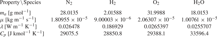
 \begin{equation} \left.\begin{array}{c} \mathcal{D}_{\textrm{N}_2\text{--}\textrm{H}_2} = 7.79236\times10^{-5} \ \textrm{m}^2\ \textrm{s}^{-1} \\ \mathcal{D}_{\textrm{N}_2\text{--}\textrm{O}_2} = 2.08575\times10^{-5} \ \textrm{m}^2\ \textrm{s}^{-1} \\ \mathcal{D}_{\textrm{N}_2\text{--}\textrm{H}_2\textrm{O}} = 2.27013\times10^{-5} \ \textrm{m}^2\ \textrm{s}^{-1} \\ \mathcal{D}_{\textrm{H}_2\text{--}\textrm{O}_2} = 8.07143\times10^{-5} \ \textrm{m}^2\ \textrm{s}^{-1} \\ \mathcal{D}_{\textrm{H}_2\text{--}\textrm{H}_2\textrm{O}} = 8.56433\times10^{-5} \ \textrm{m}^2\ \textrm{s}^{-1} \\ \mathcal{D}_{\textrm{O}_2\text{--}\textrm{H}_2\textrm{O}} = 8.07143\times10^{-5} \ \textrm{m}^2\ \textrm{s}^{-1} \end{array}\right\}. \end{equation}
C.3. Speed of sound, § 4.4

 \begin{equation} \left.\begin{array}{c} \mathcal{D}_{\textrm{H}_2\text{--}\textrm{Ar}} = 8.14543\times10^{-5} \ \textrm{m}^2\ \textrm{s}^{-1} \\ \mathcal{D}_{\textrm{H}_2\text{--}\textrm{CH}_4} = 7.37433\times10^{-5} \ \textrm{m}^2\ \textrm{s}^{-1} \\ \mathcal{D}_{\textrm{Ar}\text{--}\textrm{CH}_4} = 2.17321\times10^{-5} \ \textrm{m}^2\ \textrm{s}^{-1} \\ \mathcal{D}_{\textrm{H}_2\text{--}\textrm{C}_3\textrm{H}_8} = 4.68396\times10^{-5} \ \textrm{m}^2\ \textrm{s}^{-1} \\ \mathcal{D}_{\textrm{Ar}\text{--}\textrm{C}_3\textrm{H}_8} = 1.03862\times10^{-5} \ \textrm{m}^2\ \textrm{s}^{-1} \end{array}\right\}. \end{equation}
C.4. Kelvin–Helmholtz instability, § 4.5

 \begin{equation} \mathcal{D}_{\textrm{N}_2-\textrm{H}_2\textrm{O}} = 2.27013\times10^{-5} \ \textrm{m}^2\ \textrm{s}^{-1}. \end{equation}


 Open access