2. Model problem and numerical methods

The data is obtained from a DNS of a pressure-driven constant mass flux plane Poiseuille flow in a channel which is doubly periodic in the streamwise, $x$, and spanwise, $z$, directions. The velocity field is decomposed into the streamwise-mean component $\boldsymbol {U}=(U,V,W)$ and fluctuations from the mean, $\boldsymbol {u}=(u,v,w)$. In this decomposition the R-S is part of the mean component of the flow with the streak component defined as $U_s(y,z,t)= U-[U]$, where the square brackets $[ {\cdot }]\ {\stackrel {\mathrm {def}}=}\ (1/L_z) \int _0^{L_z} {\cdot } \, {\rm d} z$ denote the spanwise average, and the roll component has velocities components $(0,V,W)$.

The incompressible non-dimensional NSE governing the channel flow in this decomposition are

(2.1a)$$\begin{gather} \partial_t \boldsymbol{U} + \boldsymbol{U} \boldsymbol{\cdot} \boldsymbol{\nabla} \boldsymbol{U} - \varPi(t) \hat{\boldsymbol{x}} + \boldsymbol{\nabla} P - R^{{-}1} \Delta \boldsymbol{U} ={-} \overline{\boldsymbol{u} \boldsymbol{\cdot} \boldsymbol{\nabla} \boldsymbol{u}}, \end{gather}$$

(2.1b)$$\begin{gather}\partial_t\boldsymbol{u}+ \boldsymbol{U} \boldsymbol{\cdot} \boldsymbol{\nabla} \boldsymbol{u} + \boldsymbol{u} \boldsymbol{\cdot} \boldsymbol{\nabla} \boldsymbol{U} + \boldsymbol{\nabla} p- R^{{-}1} \Delta \boldsymbol{u} ={-}(\boldsymbol{u} \boldsymbol{\cdot} \boldsymbol{\nabla} \boldsymbol{u} - \overline{\boldsymbol{u} \boldsymbol{\cdot} \boldsymbol{\nabla} \boldsymbol{u}} ) , \end{gather}$$

(2.1c)$$\begin{gather}\boldsymbol{\nabla} \boldsymbol{\cdot} \boldsymbol{U} = 0, \quad \boldsymbol{\nabla} \boldsymbol{\cdot} \boldsymbol{u} = 0. \end{gather}$$

The pressure gradient $\varPi (t)$ is adjusted in time to maintain constant mass flux. Lengths have been made non-dimensional by $h$, the channel's half-width, velocities by the time-mean velocity at the centre of the channel, $U_c$, and time by $h/ U_c$. Averaging in $x$ is denoted by $\overline {( {\cdot } )}$ and averaging in time by $\langle {\cdot } \rangle$. No-slip and impermeable boundaries are placed at $y = 0$ and $y = 2$, in the wall-normal variable. The Reynolds number is $R= U_c h / \nu$, with $\nu$ the kinematic viscosity.

The DNS is obtained using NSE (2.1) and for comparison, parallel simulations are made with the RNL approximation of (2.1), which is obtained by parameterizing the fluctuation–fluctuation nonlinearity in (2.1b). The parameterization used is to set these nonlinear interactions among streamwise non-constant flow components in the fluctuation equations (2.1b) to zero. Consequently, the RNL system of equations is

(2.2a)$$\begin{gather} \partial_t\boldsymbol{U}+ \boldsymbol{U} \boldsymbol{\cdot} \boldsymbol{\nabla} \boldsymbol{U} - \varPi(t) \hat{\boldsymbol{x}} + \boldsymbol{\nabla} P - R^{{-}1}\Delta \boldsymbol{U} ={-} \overline{\boldsymbol{u} \boldsymbol{\cdot} \boldsymbol{\nabla} \boldsymbol{u}} , \end{gather}$$

(2.2b)$$\begin{gather}\partial_t\boldsymbol{u}+ \boldsymbol{U} \boldsymbol{\cdot} \boldsymbol{\nabla} \boldsymbol{u}+ \boldsymbol{u} \boldsymbol{\cdot} \boldsymbol{\nabla} \boldsymbol{U} + \boldsymbol{\nabla} p- R^{{-}1} \Delta \boldsymbol{u} = 0. \end{gather}$$

(2.2c)$$\begin{gather}\boldsymbol{\nabla} \boldsymbol{\cdot} \boldsymbol{U} = 0, \quad \boldsymbol{\nabla} \boldsymbol{\cdot} \boldsymbol{u} = 0. \end{gather}$$

Under this quasilinear restriction, the fluctuation field interacts nonlinearly only with the mean, $\boldsymbol {U}$, flow and not with itself. This quasilinear restriction of the dynamics results in the spontaneous collapse in the support of the fluctuation field to a small subset of streamwise Fourier components, while maintaining conservation of the total flow energy $1/2 \int _{\mathcal {D}} d^3 \boldsymbol {x} ( |\boldsymbol {U}|^2 + |\boldsymbol {u}|^2 )$ in the absence of dissipation ($\mathcal {D}$ is the flow domain). This restriction in the support of RNL turbulence to a small subset of streamwise Fourier components is not imposed but rather is a property of the quasilinear dynamics. The fluctuation components retained by the dynamics identify the streamwise harmonics that are energetically active in the parametric growth process that sustains the fluctuations (Farrell & Ioannou Reference Farrell and Ioannou2012; Constantinou, Farrell & Ioannou Reference Constantinou, Farrell and Ioannou2014; Thomas et al. Reference Thomas, Lieu, Jovanović, Farrell, Ioannou and Gayme2014, Reference Thomas, Farrell, Ioannou and Gayme2015; Farrell et al. Reference Farrell, Ioannou, Jiménez, Constantinou, Lozano-Durán and Nikolaidis2016). In a DNS at $R=2250$ these energetically active streamwise harmonics have been shown to synchronize the remaining components (Nikolaidis & Ioannou Reference Nikolaidis and Ioannou2022).

The data were obtained from a DNS of (2.1), referred to as NSE100, and from the associated RNL governed by (2.2), referred to as RNL100. The Reynolds number $R = U_c h/\nu =1650$ is imposed in both the DNS and the RNL simulations. A summary of the parameters of the simulations is given in table 1. The RNL100 simulation is supported by only three streamwise components with wavelengths $\lambda _x/h = 4 {\rm \pi}, 2 {\rm \pi}, 4{\rm \pi} /3$, which correspond to the three lowest streamwise Fourier components of the channel, $n_x=1,2,3$.

Table 1. Simulation parameters: $[L_x,L_z]/h$ is the domain size in the streamwise, spanwise direction; $[\alpha,\beta ] = [2{\rm \pi} /L_x, 2{\rm \pi} /L_z]$ denote the fundamental wavenumbers in the streamwise and spanwise directions; $N_x$, $N_z$ are the number of Fourier components after dealiasing and $N_y$ is the number of Chebyshev components; $R_\tau = u_\tau h / \nu$ is the Reynolds number of the simulation based on the friction velocity $u_\tau = \sqrt { \nu \,\textrm {d} [ U ] /\textrm {d} y|_{w}}$, where $\textrm {d} [ U ] /\textrm {d} y|_{w}$ is the shear at the wall.

For the numerical integration the dynamics were expressed in the form of evolution equations for the wall-normal vorticity and the Laplacian of the wall-normal velocity, with spatial discretization and Fourier dealiasing in the two wall-parallel directions and Chebychev polynomials in the wall-normal direction (Kim, Moin & Moser Reference Kim, Moin and Moser1987). Time stepping was implemented using the third-order semi-implicit Runge–Kutta method.

3. Obtaining the streamwise-mean R-S and the covariance of the associated fluctuations using collocation

In order to analyse the dynamics of the R-S we obtain both the streamwise-mean R-S and the time-mean spatial two-point covariances of the fluctuations collocated with the R-S for both the high-speed and the low-speed streak. The collocation implementation is described in Nikolaidis et al. (Reference Nikolaidis, Ioannou, Farrell and Lozano-Durán2023). Briefly the method proceeds by identifying the spanwise location of the streak with the location of the spanwise coordinate of the $\min (U_s)$ (for low-speed streaks) and translating the entire flow field in the spanwise direction to place the low-speed streak minimum at the channel centre $z/h=0$. We have verified that as the averaging time increases the time-mean streak approaches mirror symmetry in the spanwise about the streak centreline. We enforce this symmetry in the dataset and double the available data by symmetrizing about the aligned streak centre.

The time-mean streak, $\langle U_s \rangle$, obtained from the aligned time series of $\min (U_s)$ isolates the low-speed streak, producing a coherent low-speed R-S at $z/h=0$, while away from this core region the velocity components cancel indicative of their being incoherently correlated with the centred streak. This collocation procedure is similarly implemented to isolate the high-speed streak. 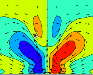The structures in the $y$–$z$ plane of the time-mean low-speed and high-speed R-S in NSE100 are shown in figure 1(a,b) using contours for $\langle U_s \rangle$ and vectors for $(\langle W \rangle,\langle V \rangle )$. The time-mean flow in the upper region, $y/h>1$, is to a good approximation spanwise homogeneous (not shown). The structure of the time-mean streaks in RNL100 are similar (cf. Nikolaidis et al. Reference Nikolaidis, Ioannou, Farrell and Lozano-Durán2023). It is important to note that although low-speed streaks are associated with flanking high-speed streak components, the low-speed streaks are isolated structures in the statistical mean because of the decoherence of the spanwise location of the streaks in Poiseuille flow. In contrast, simulations of Couette flow turbulence in wide channels reveal that the streaks exhibit long range correlation (Avsarkisov et al. Reference Avsarkisov, Hoyas, Oberlack and Garcia-Galache2014; Pirozzoli et al. Reference Pirozzoli, Bernardini and Orlandi2014; Lee & Moser Reference Lee and Moser2018). The implication is that in wide channel Couette flow a collocation procedure would not be necessary because the turbulence would exhibit a full array of spanwise periodic low- and high-speed R-S rather than the random distribution of isolated R-S seen in Poiseuille flow.

Figure 1. Contours of the time-mean collocated streak, $\langle U_s \rangle$, and vectors of the roll velocity, $(\langle W \rangle,\langle V \rangle )$, for the NSE100 low-speed streak (a) and high-speed streak (b). The contour interval is 0.025. In (a) the $\max (|\langle U_s \rangle |) = 0.21 U_c$, $\max (\langle V \rangle )=0.024 U_c$. In (b) the $\max (|\langle U_s \rangle |) = 0.16 U_c$, $\max (\langle V \rangle )=0.015 U_c$. The contour interval is $0.025 U_c$.

Having isolated at each time instant the streamwise-mean R-S with streamwise velocity $U(y,z,t)$, wall-normal velocity $V(y,z,t)$ and spanwise velocity $W(y,z,t)$, we Fourier decompose in the streamwise direction the fluctuation velocities collocated with the streak

(3.1)\begin{equation} \boldsymbol{u}= [ u(\boldsymbol{x},t), v(\boldsymbol{x},t), w(\boldsymbol{x},t)]^T, \end{equation}

and calculate the time-mean covariance

(3.2)\begin{equation} {\boldsymbol C}_{k_x}(y_1,z_1,y_2,z_2) =\langle \boldsymbol{u}_{k_x}(y_1,z_1) \boldsymbol{u}_{k_x}^{{{\dagger}}}(y_2,z_2) \rangle, \end{equation}

where ${\boldsymbol {u}}_{k_x}(y_i,z_i))$ is the amplitude of the $n_x$th Fourier component of the velocity field with streamwise wavenumber, $k_x= n_x \alpha$, at the position $(y_i,z_i)$, with ${\dagger}$ indicating the Hermitian transpose and $\alpha =2 {\rm \pi}/L_x$ the smallest streamwise wavenumber in the channel. The same point time-mean covariance is denoted ${\boldsymbol C}_{k_x} (y,z)$. From this time-mean covariance we obtain the time-mean Reynolds stresses produced by the fluctuations.

4. The R-S dynamical balance diagnostics

The time-mean collocated R-S and the associated time-mean collocated fluctuation Reynolds stresses comprise components of the structure of the R-S and the dynamics maintaining it, respectively. We will now examine the terms in this equilibrium for the case of the low-speed streak.

Equations (2.1a) and (2.2a) imply that the streamwise-mean streak, $U_s=U-[U]$, satisfies the equation

(4.1)\begin{align} \partial_t U_s ={-} (V \partial_y (U)- [V \partial_y U])- W \partial_z U_s -\partial_y (\overline{u v} - [\overline{u v}])- \partial_z (\overline{u w} - [\overline{u w}])+ R^{{-}1} \Delta U _s, \end{align}

so that, given that $\partial _z [\overline {u w}]=0$, the time-mean streak satisfies the force balance:

(4.2)\begin{align} - \langle (V \partial_y (U)- [V \partial_y U]) \rangle - \langle W \partial_z U_s \rangle -\partial_y( \langle \overline{u v} \rangle-\langle [\overline{u v}] \rangle ) - \partial_z \langle \overline{u w} \rangle + R^{{-}1} \Delta \langle U _s \rangle = 0.\end{align}

The terms comprising this balance are verified to be in a time-mean equilibrium in figure 2, for the NSE100, and in figure 3, for the RNL100. Moreover, figures 2 and 3 show that, in the time-mean, the streak is principally supported by the lift-up mechanism, $- \langle V \partial _y U -[V\partial _y U] \rangle$, and opposed by spanwise Reynolds stress divergence, $-\partial _z \langle \overline {u w} \rangle$ and diffusion $R^{-1} \Delta \langle U _s \rangle$.

Figure 2. For the low-speed streak in NSE100, contours in the $(y,z)$ plane are shown for (a) $- \langle V \partial _y U - [V \partial _y U] \rangle$, (b) $- \langle W \partial _z U_s \rangle$, (c) $-\langle \partial _y (\overline {u v} -[\overline {uv}])\rangle$, (d) $- \partial _z \langle \overline {u w} \rangle$ and (e) $R^{-1} \Delta \langle U _s \rangle$. The sum shown in (f) confirms that the above terms are in balance. The contour interval is $0.003U_c^2/h$.

Figure 3. As in figure 2 for RNL100. The contour interval is $0.003~U_c^2/h$.

A typical time series of the average amplitude of the low-speed streak at the centreline of the streak and of the principal terms in the force balance (4.2) which are the instantaneous average streak acceleration by the lift-up process, $-\int _0^1 {{\rm d} y} (V \partial _y U - [V \partial _y U])$, the average acceleration by spanwise Reynolds stress divergence, $-\int _0^1 {{\rm d} y} \partial _z \overline {uw}$, and the average acceleration due to diffusion, $R^{-1} \int _0^1\,{{\rm d} y}\Delta U_s$, are shown in figure 4. The time-mean acceleration and standard deviation over the entire dataset due to lift up is $-0.01 U_c^2/h$ (dashed blue) with $\sigma =0.004~U_c^2/h$, that due to Reynolds stress divergence is $0.007 U_c^2/h$ (dashed black) with $\sigma =0.004 U_c^2/h$ and that due to diffusion is $0.003 U_c^2/h$ (dashed green) with $\sigma =0.0013 U_c^2/h$. Over the entire dataset the acceleration due to lift up and that due to Reynolds stress divergence, $-\int _0^1 {{\rm d} y} \partial _z \overline {uw}$, are strongly correlated with cross-correlation coefficient $0.72$ at lag $1.2 h / U_c$ as shown in figure 5. Also, over the entire dataset streak maxima lead the streak regulation term, $-\int _0^h\, {\rm d} y \partial _z (\overline {uw})/(h^2 U_c^2)$, by $2 h/U_c$. Two bursting events are seen in figure 4 associated with the streak maxima at $3275 h/U_c$ and $3866 h / U_c$. These streak maxima are followed by maxima of the streak regulation term $-\int _0^h\, {\rm d} y \partial _z (\overline {uw})/(h^2 U_c^2)$ at $3282 h/U_c$ and $3879 h / U_c$, respectively. The near balance and near synchronicity seen in figure 5 indicates that the maintenance and regulation of the streak amplitude is occurring at all times and that breakdown events are not primarily responsible for either the maintenance or the regulation of the streak (see also figure 6).

Figure 4. Contributions to streak maintenance and regulation in NSE100. The scaled average streak amplitude at the centreline of the low-speed streak ($0.2 \int _0^h {{\rm d} y} U_s /h U_c$) is shown in red. The average streak acceleration by lift-up at the centreline of the low-speed streak ($-\int _0^h {{\rm d} y} (V \partial _y (U)-[V \partial _y U])/ (h^2 U_c^2)$) (blue) is opposed by the acceleration due to diffusion (green) ($R^{-1} \int _0^h {{\rm d} y}\Delta U_s/(h^2 U_c^2)$) and downgradient momentum transport by the streamwise varying fluctuations (black) ($-\int _0^h\, {\rm d} y \partial _z (\overline {uw})/(h^2 U_c^2)$). The dashed lines with the corresponding colours indicate the mean values taken over the entire dataset. This figure shows that maintenance and regulation of the streak is occurring continuously in time and is not confined to bursting events.

Figure 5. Comparison between the primary components maintaining and regulating the low-speed streak in NSE100. Shown are the acceleration due to lift-up (blue) and the negative of the acceleration due to Reynolds stress divergence (black) (cf. figure 4). The time series have been shifted by the $1.2 h/U_c$ lag between them which was obtained over the entire dataset. These two accelerations are highly correlated (correlation coefficient $0.72$) revealing that a tight quasiequilibrium between lift-up and downgradient momentum transfer characterizes the maintenance and regulation of the streak amplitude.

Figure 6. Typical section of the time series of the integrated correlation between the instantaneous value of the streamwise-mean vorticity and the streamwise-mean vorticity source $G$, $\int _0^1 \,{{\rm d} y} [ \varOmega _x G ] h^2/U_c^3$, for the case of the low-speed streak in NSE10. Over the whole dataset the time mean is $0.0035 h^2/U_c^3$ (dashed). This figure shows that the forcing of the roll, and consequently of the streak, is continuous in time and almost always positive.

5. Maintenance of the streamwise-mean roll

Having verified the dominance of lift-up by roll circulations in supporting the R-S, our attention turns to studying the mechanism giving rise to the remarkable universal coincidence in wall turbulence of streaks with roll circulations properly configured to maintain them. By taking the curl of the streamwise-mean equations (2.1a) and (2.2a) we obtain that in both NSE100 and RNL10 the streamwise component of the vorticity $\varOmega _x = \partial _y W - \partial _z V$ satisfies the equation

(5.1)\begin{equation} \partial_t \varOmega_x = \underbrace{-(V \partial_y + W \partial_z) \varOmega_x}_A +\underbrace{(\partial_{zz} - \partial_{yy}) \overline{v w}+ \partial_{yz}(\overline{v^2} -\overline{w^2})}_{G} + \underbrace{R^{{-}1} \Delta \varOmega_x}_D, \end{equation}

in which the streamwise-mean wall-normal and spanwise velocities are given by $V=-\partial _z \varDelta ^{-1} \varOmega _x$ and $W=\partial _y \varDelta ^{-1} \varOmega _x$ with the inverse Laplacian $\varDelta ^{-1}$ incorporating the boundary conditions.

The term $A$, representing advection of $\varOmega _x$ by the roll velocities $(V,W)$, is not a source of net streamwise vorticity. The roll vorticity is sustained against dissipation, $D$, by the curl of the force arising from the Reynolds stress divergence, $G$. In this equation the wall-normal component of the Reynolds stress divergence force is

(5.2)\begin{equation} F_y={-}\partial_z( \overline{v w})- \partial_y ( \overline{v^2}), \end{equation}

while the spanwise component is

(5.3)\begin{equation} F_z={-}\partial_y ( \overline{v w})- \partial_z ( \overline{w^2}), \end{equation}

which results in the contribution to the rate of change of streamwise-mean vorticity in the streamwise direction:

(5.4)\begin{equation} G=\widehat{\boldsymbol{x}} \boldsymbol{\cdot} \boldsymbol{\nabla} \times (0,F_y,F_z) = ( \partial_{zz} -\partial_{yy} )\overline{vw}+ \partial_{yz} ( \overline{v^2} - \overline{w^2} ),\end{equation}

where $\widehat {\boldsymbol {x}}$ is the unit vector in the streamwise direction. The first right-hand side term in (5.4) represents the contribution to $G$ from the Reynolds shear stress $\overline {vw}$, while the second term represents the contribution from $\overline {v^2} - \overline {w^2}$, which can be identified with anisotropy in the Reynolds normal stress components. The implications of this decomposition are discussed by Alizard et al. (Reference Alizard, Le Penven, Cadiou, Di Pierro and Buffat2021) in the context of the formation of streamwise constant rolls during transition to turbulence in the RNL framework. The Reynolds normal stress component of $G$ will be shown in the next section to dominate and determine the direction and location of the roll circulation and consequently of the streak acceleration.

A time series of the inner product of $\varOmega _x$ with $G$ is shown in figure 6. Two observations are appropriate: the first is that roll forcing by Reynolds stresses is continuous in time and almost always positive; the second is that streamwise-mean vorticity forcing is negatively associated with bursting events such as that occurring around $t=3800$. Continual generation of streamwise vorticity supporting the existing roll circulation both in the buffer layer and also in the logarithmic layer was previously documented in RNL turbulence at Reynolds number $R_\tau =1000$ (cf. Farrell et al. Reference Farrell, Ioannou, Jiménez, Constantinou, Lozano-Durán and Nikolaidis2016). This result has not yet been confirmed in DNS, but we expect it to be, given that parallel mechanisms underlie wall turbulence in RNL and DNS.

In the time-mean the streamwise-mean vorticity, $\varOmega _x$, satisfies the balance

(5.5)\begin{equation} \underbrace{- \langle (V \partial_y + W \partial_z) \varOmega_x \rangle}_{\langle A \rangle}+ \underbrace{(\partial_{zz} - \partial_{yy}) \langle \overline{v w} \rangle + \partial_{yz} \langle (\overline{v^2} -\overline{w^2})\rangle}_{\langle G \rangle} + \underbrace{R^{{-}1} \Delta \langle \varOmega_x \rangle}_{\langle D \rangle} = 0.\end{equation}

The three components of this time-mean balance in NSE100 and RNL100 are shown in figures 7 and 8.

Figure 7. For the low-speed streak in NSE100, contours in the $(y,z)$ plane are shown for (a) $\langle A \rangle =-\langle (V \partial _y + W \partial _z) \varOmega _x \rangle$, contribution to the time-mean rate of change of $\langle \varOmega _x \rangle$ by roll self-advection, (b) $\langle G \rangle =(\partial _{zz} - \partial _{yy}) \langle \overline {v w} \rangle + \partial _{yz} \langle (\overline {v^2} -\overline {w^2})\rangle$, contribution to the time-mean rate of change of $\langle \varOmega _x \rangle$ by Reynolds stress divergence, (c) $\langle D \rangle =R^{-1} \Delta \langle \varOmega _x \rangle$, contribution to the time-mean rate of change of $\langle \varOmega _x \rangle$ by dissipation. The sum shown in (d) confirms that the above terms are in balance. The contour interval is $0.0015U_c^2/h$.

Figure 8. As in figure 7 for RNL100. The contour interval is $0.0015 U_c^2/h$.

The roll circulation resulting from the forcing by $\langle G \rangle$ can be understood by assessing the wall-normal velocity induced by $\langle G \rangle$ together with its modification by $\langle A \rangle$. The modification given by $\langle A \rangle$ results from a pressure field required so that the circulation forced by $\langle G \rangle$ satisfies boundary conditions. We project (5.5) to streamwise-mean wall-normal velocity by multiplying (5.5) with $-\delta t \partial _z \varDelta ^{-1}$ for a chosen time interval $\delta t$ in order to obtain

(5.6)\begin{equation} \delta V_A + \delta V_G ={-} \delta t R^{{-}1} \Delta \langle V \rangle, \end{equation}

where $\delta V_G = -\delta t \partial _z \varDelta ^{-1} \langle G \rangle$ is the wall-normal velocity increment induced by $\langle G \rangle$ over time interval $\delta t$ and $\delta V_A = -\delta t \partial _z \varDelta ^{-1} \langle A \rangle$ is the corresponding wall-normal velocity increment induced by $\langle A \rangle$. It is the $\delta V_G$ induced by $\langle G \rangle$ and corrected by $\delta V_A$ that determines the equilibrium $V$ field as indicated in the balance equation (5.6). The wall-normal velocity increments $\delta V_G$ and $\delta V_A$ maintaining the low-speed R-S in NSE100 are shown in figure 9. This figure shows that $\delta V_G$ is providing lift-up in the streak core supporting the low-speed R-S and also the corrective $\delta V_A$, which is approximately $1/3$ of the $\delta V_G$, is adding to the support of the R-S provided by $\langle G \rangle$.

Figure 9. For the low-speed streak in NSE100, contours in the $(y,z)$ plane are shown for (a) the time-mean wall-normal velocity increment resulting from advection, $\delta V_A$, (b) the wall-normal velocity increment resulting from Reynolds stress, $\delta V_G$, and (c) their sum $\delta V_A+ \delta V_G$. This figure shows the contribution of the advection and Reynolds stress to the maintenance of the low-speed R-S. The associated $\langle A \rangle$, $\langle G \rangle$ fields are shown in figure 7(a,b). The contour interval is $2\times 10^{-4} U_c$.

In figure 9 we have taken the time interval for the development of $\delta V$ to be ${\delta t=1 h/U_c}$; however, it is instructive to identify a physically relevant value of this time scale which for the low-speed streak is given by $T_d/\delta t \approx V_{max}/ \delta V_{max}=12$, where $V_{max}$ is the maximum wall normal velocity at the streak centreline (cf. figure 1a) and $\delta V_{max}$ is the maximum wall-normal velocity increment over unit time also evaluated at the centreline (cf. figure 9c). This time scale can be interpreted as a Rayleigh damping time scale for equilibration of the roll circulation being forced by the Reynolds stresses.

6. Contribution to roll forcing by the sinuous ($\mathcal {S}$) and varicose ($\mathcal {V}$) fluctuations

In the previous section we showed that the Reynolds stresses induce vorticity forcing that continuously reinforces the pre-existing streamwise-mean streamwise vorticity so as to sustain the R-S. Key to understanding this remarkable property is the dynamics of the ${\mathcal {S}}$ and ${\mathcal {V}}$ fluctuations collocated with the mean streak. In this section we isolate the $\mathcal {S}$ and $\mathcal {V}$ components of the velocity fluctuations collocated with the streak and show that the maintenance of the mean R-S can be attributed to the Reynolds stresses due to the ${\mathcal {S}}$ and ${\mathcal {V}}$ components of velocity acting independently. Although instantaneous snapshots of the flow field would reveal Reynolds stresses arising from interaction between the ${\mathcal {S}}$ and ${\mathcal {V}}$ fields, this interaction vanishes in the time-mean. This is expected because the R-S is mirror-symmetric, and non-vanishing of the time-mean ${\mathcal {S}}$ and ${\mathcal {V}}$ covariance would result in Reynolds stresses incompatible with the mirror symmetry of the time-mean R-S – this will be verified below.

In order to define the time-mean covariance of the ${\mathcal {S}}$ and ${\mathcal {V}}$ components of the fluctuation field we form at each time step of the simulation the ${\mathcal {S}}$ and ${\mathcal {V}}$ components of the velocity field:

(6.1)\begin{equation} \boldsymbol{u}_{\mathcal{S}} (x,y,z,t) = \frac{\boldsymbol{u} - \boldsymbol{u}_{mirror}}{2}, \boldsymbol{u}_{\mathcal{V}} (x,y,z,t) = \frac{\boldsymbol{u} + \boldsymbol{u}_{mirror}}{2} , \end{equation}

in which the mirror symmetric fluctuation field about the plane $z=0$ is defined as

(6.2)\begin{equation} {\boldsymbol{u}}_{mirror}(x,y,z,t) {\stackrel{\mathrm{def}}=} \begin{pmatrix} u(x,y,-z,t) \\ v(x,y,-z,t) \\ -w(x,y,-z,t) \end{pmatrix}. \end{equation}

The time-mean spatial covariances of the ${\mathcal {S}}$ and ${\mathcal {V}}$ components of the fluctuation field at streamwise wavenumber $k_x$ are ${\boldsymbol C}_{{\mathcal {S}}, k_x}(y_1,z_1,y_2,z_2) {\stackrel {\mathrm {def}}=}\langle {\boldsymbol {u}}_{{\mathcal {S}}, k_x}(y_1,z_1) {\boldsymbol {u}}_{{\mathcal {S}}, k_x}^{{\dagger} }(y_2,z_2) \rangle$ and ${\boldsymbol C}_{{\mathcal {V}}, k_x}(y_1,z_1,y_2,z_2) {\stackrel {\mathrm {def}}=}\langle {\boldsymbol {u}}_{{\mathcal {V}}, k_x}(y_1,z_1) {\boldsymbol {u}}_{{\mathcal {V}}, k_x}^{{\dagger} }(y_2,z_2) \rangle$, where $\boldsymbol {u}_{{\mathcal {S}}/{\mathcal {V}},k_x}$ are the Fourier amplitudes of the ${\mathcal {S}}$ and ${\mathcal {V}}$ components of the fluctuation velocity field at $k_x$, while the corresponding covariance of the total field is given by ${\boldsymbol C}_{k_x}(y_1,z_1,y_2,z_2) {\stackrel {\mathrm {def}}=}\langle {\boldsymbol {u}}_{k_x}(y_1,z_1) {\boldsymbol {u}}_{k_x}^{{\dagger} } (y_2,z_2) \rangle$. The asymptotic approach in time of the equality

(6.3)\begin{equation} {\boldsymbol C}_{k_x}(y_1,z_1,y_2,z_2)={\boldsymbol C}_{{\mathcal{S}}, k_x}(y_1,z_1,y_2,z_2) +{\boldsymbol C}_{{\mathcal{V}}, k_x}(y_1,z_1,y_2,z_2) \end{equation}

has been verified, implying that there is no time-mean correlation between the ${\mathcal {S}}$ and ${\mathcal {V}}$ fluctuations. Consequently, the time-mean fluctuation Reynolds stresses, which are a linear function of the covariances, are the sum of the Reynolds stresses obtained from the respective ${\mathcal {S}}$ and ${\mathcal {V}}$ covariances. The fluctuation Reynolds stress can be further partitioned into a sum over $k_x$. Using this partition into ${\mathcal {S}}$ and ${\mathcal {V}}$ components at each wavenumber $k_x$, we can separate the contribution of the ${\mathcal {S}}$ and ${\mathcal {V}}$ components at each $k_x$ to the mechanism sustaining the R-S.

We turn now to study how the roll is induced by the time-mean fluctuation Reynolds stresses. We first consider the contribution to the roll forcing by the time-mean Reynolds stresses due to $k_x$ fluctuations, $\langle G_{k_x} \rangle =(\partial _{zz} - \partial _{yy}) \langle \overline {v w} \rangle _{k_x} + \partial _{yz} \langle (\overline {v^2} -\overline {w^2})\rangle _{k_x}$. This $\langle G_{k_x} \rangle$ acting alone would result, as discussed in the previous section, in a wall-normal velocity increment over time $\delta t$, $\delta V_{k_x} = -\delta t \partial _z \varDelta ^{-1} \langle G_{k_x} \rangle$, and a spanwise velocity increment over time $\delta t$, $\delta W_{k_x} =\delta t \partial _y \varDelta ^{-1} \langle G_{k_x} \rangle$. The associated streamwise-mean vorticity increment is $\delta \varOmega _{x,k_x}=\langle G_{k_x} \rangle \delta t$ and $\varDelta ^{-1}$ the inverse Laplacian required to account for the influence of pressure forces arising from the boundary conditions. We choose $\delta t = 1$ from now on.

The spatial distribution of $\delta \varOmega _{x,k_x}$ and vector plots of the streamwise-mean velocity fields $(\delta V_{k_x}, \delta W_{k_x})$ induced by ${\mathcal {S}}$ and ${\mathcal {V}}$ components of $k_x=3 \alpha$ fluctuations in NSE100 for the case of the low-speed streak are shown in figure 10. Note that the velocity increment vectors are not tangent to the contours of the vorticity increments, $\delta \varOmega _{x,k_x}$. This is due to the action of pressure forces arising due to the boundary conditions. This figure demonstrates that ${\mathcal {S}}$ Reynolds stresses produce mean vorticity that reinforces the low speed streak while the ${\mathcal {V}}$ Reynolds stresses oppose the low-speed streak. In low-speed streaks the ${\mathcal {S}}$ Reynolds stresses dominate, consistent with the ${\mathcal {S}}$ structures maintaining the low-speed streak. While both ${\mathcal {S}}$ and ${\mathcal {V}}$ fluctuations are present in association with low-speed streaks so that application of targeted data analysis techniques could be used to deduce the presence of, for example, hairpin vortex structures in association with low-speed streaks, this result demonstrates that the varicose component at $k_x= 3 \alpha$ opposes rather than maintains the low-speed streak. We will verify that this is also the case at other $k_x$. Conversely, in high-speed streaks the ${\mathcal {V}}$ Reynolds stresses dominate, consistent with maintaining the high-speed streak. We will show that this is also a general property. In RNL100 we obtain similar results (cf. figure 11).

Figure 10. Increment of mean streamwise vorticity, $\delta {\varOmega }_{x,k_x}$, induced over unit time by Reynolds stresses of the $\mathcal{S}$ (a) and the $\mathcal{V}$ (b) $k_x/\alpha =3$ fluctuations in the low-speed streak of NSE100. Wavenumber $k_x/\alpha =3$ is chosen because the forcing is maximized at this wavenumber (cf. figure 12a). Also shown are vectors with components $(\delta W_{k_x}, \delta V_{k_x})$. This figure shows that the ${\mathcal {S}}$ fluctuations reinforce the low-speed streak while the $\mathcal {V}$ fluctuations oppose it. Overall the ${\mathcal {S}}$ fluctuations are dominant and the low-speed streak is sustained.

Figure 11. Increment of mean streamwise vorticity, $\delta {\varOmega }_{x,k_x}$, induced over unit time by Reynolds stresses of the ${\mathcal {S}}$ (a) and the ${\mathcal {V}}$ (b) $k_x/\alpha =2$ fluctuations that are collocated with the mean low-speed streak in RNL100. Wavenumber $k_x/\alpha =2$ is chosen because the forcing is maximized at this wavenumber (cf. figure 13a). Also shown are vectors with components the roll velocities induced over unit time $(\delta W_{k_x}, \delta V_{k_x})$. This figure shows that the ${\mathcal {S}}$ fluctuations reinforce the low-speed streak while the ${\mathcal {V}}$ fluctuations oppose it as in NSE100 shown in figure 10.

The velocity increment forced by the Reynolds stresses over the primary area of lift-up forcing (see figure 9b)

(6.4)\begin{equation} \widetilde {\delta V}_{k_x} {\stackrel{\mathrm{def}}=} \int_{{-}z_0}^{z_0} \frac{{\rm d}z}{2 z_0} \int_0^{y_0} \frac{{\rm d} y}{y_0} \delta V_{k_x}(y,z), \end{equation}

with $y_0=h/2$ and $z_0=0.26 h$, partitioned into ${\mathcal {S}}$ and ${\mathcal {V}}$ components, and the velocity increment induced by their sum, ${\mathcal {S}}+{\mathcal {V}}$, as a function of the streamwise wavenumber of the fluctuations, $k_x/\alpha$, for the case of the low-speed streak and the high-speed streak in NSE100 is shown in figure 12. The corresponding RNL100 results shown in figure 13 are similar to those of the NSE100, except that in RNL100 the streak is supported by only the first three streamwise wavenumbers, which are the streamwise wavenumbers spontaneously retained by RNL dynamics. These figures show that in the time-mean and at all streamwise wavenumbers considered, the $\mathcal {S}$ fluctuations induce lift-up in both low- and high-speed streaks, while the $\mathcal {V}$ induce push-down. These figures also show that in low-speed streaks the $\mathcal {S}$ component dominates the $\mathcal {V}$ at every $k_x$ resulting in the support of the low-speed streak, while in high-speed streaks the $\mathcal {V}$ component dominates the $\mathcal {S}$ resulting in the support of the high-speed streak. Also the contribution to roll forcing by the fluctuations at each wavenumber is similarly distributed so that each wavenumber is contributing to the reinforcement of the pre-existing R-S. Note that the Reynolds stress induced time-mean $\widetilde { \delta V}_{k_x}$ is maximized at $k_x/\alpha =3$ for both low-speed and high-speed streaks in NSE100. However, the support of the streak extends over a broad band of streamwise wavenumbers implying structural robustness of the mechanism of roll forcing supporting the SSP cycle in wall turbulence.

Figure 12. Velocity increments, $\widetilde {\delta V}_{k_x}$, forced by the Reynolds stresses over the primary area of lift-up, partitioned into ${\mathcal {S}}$ and ${\mathcal {V}}$ components, and the velocity increment induced by their sum, ${\mathcal {S}}$ + ${\mathcal {V}}$, as a function of the streamwise wavenumber of the fluctuations, $k_x/\alpha$, for the case of the low-speed streak (a) and the high-speed streak (b) of NSE100. The largest induced velocity occurs at $k_x/\alpha =3$ for both the low-speed streak and high-speed streak. These figures show that in the time-mean the ${\mathcal {S}}$ fluctuations induce lift-up while the ${\mathcal {V}}$ induce push-down. In the low-speed streak the $\mathcal {S}$ induced lift-up dominates the $\mathcal {V}$ push-down producing maintenance of the low-speed streak, while in the high-speed streak the $\mathcal {V}$ induced lift-up dominates the $\mathcal {S}$ push-down producing maintenance of the high-speed streak.

Figure 13. As in figure 12 except RNL100.

Note that the wall-normal velocity increments induced either by the $\mathcal {S}$ or the $\mathcal {V}$ fluctuations in the case of the low-speed streak are substantially larger than the corresponding velocity increments induced for the case of the high-speed streak. Moreover, the net roll forcing from the sum of the opposing ${\mathcal {S}}$ and $\mathcal {V}$ induced velocities is approximately two times larger in the low-speed streak compared with the high-speed streak. This dynamical advantage in forcing of the low-speed streak in comparison with the forcing of the high-speed streak, combined with the increased dissipation resulting from displacement of the high-speed streak towards the boundary, provides explanation for the relative dominance of the low-speed streak in observations of isolated R-S as occur in this Poiseuille flow. In the case of the highly ordered R-S observed in wide channel Couette flow (Pirozzoli et al. Reference Pirozzoli, Bernardini and Orlandi2014), the low- and high-speed streaks would not be independent and their interaction would need to be taken into account.

7. Contribution to streak forcing by the ${\mathcal {S}}$ and $\mathcal {V}$ shear and normal Reynolds stress components

Simplicity in analysing the mechanism by which the Reynolds stress forcing $G$ gives rise to the R-S can be obtained by concentrating on the forcing of $V$ along the centreline of the streak given by $\delta V_{k_x}(y,z=0)$. The $y$ structure of the $\mathcal {S}$ and $\mathcal {V}$ components of $\delta V_{k_x}(y,z=0)$ for the low-speed streak in NSE100 is shown in figure 14. This figure shows that the Reynolds stress induced lift-up at each wavenumber add coherently.

Figure 14. Wall-normal distribution at the centreline of $\delta V_{k_x}(y,z=0)$. Shown separately are the ${\mathcal {S}}$ (a) and the ${\mathcal {V}}$ (b) components with streamwise wavenumber $k_x/\alpha =1,2,\ldots,12$ for the case of the low-speed streak of NSE100.

For the analysis of the streak forcing we choose to show the streak velocity at the streak centreline induced by $\delta V_{k_x}(y,0)$ acting over unit time, $\delta U = - \delta V_{k_x}(y,0) U'(y,0) \delta t$, with $\delta t=1$ and $U'(y,0)$ the shear of the streamwise flow at the streak centreline. The streak velocity $\delta U$ induced by the dominant $k_x/\alpha =3$ fluctuations is plotted in figure 15 for the low-speed streak in NSE100 and in figure 16 for the high-speed streak in NSE100, both of which are located in the lower half of the channel by our collocation procedure. The net $\delta U$ induced in the upper half of the channel by the $\mathcal {S}$ and $\mathcal {V}$ fluctuations, where there is no streak, vanishes in the time-mean. In the lower region, where there is a streak, the ${\mathcal {S}}$ and $\mathcal {V}$ contributions do not cancel in the time-mean and a net $\delta U$ results. In the low-speed streak region of figure 15(a), the $\mathcal {S}$ fluctuations dominate the $\mathcal {V}$ fluctuations in the time-mean resulting in $\delta U$ increments supporting the low-speed streak. In general it can be shown that $\mathcal {S}$ fluctuations force low-speed streaks while $\mathcal {V}$ fluctuations oppose this forcing (Farrell, Ioannou & Nikolaidis Reference Farrell, Ioannou and Nikolaidis2022). In the high-speed streak regions, as shown in figure 16(a), the high-speed streak is forced by the Reynolds stresses of $\mathcal {V}$ fluctuations which dominate the opposing tendency of the $\mathcal {S}$ fluctuations. The induced $\delta U$ in RNL100 are similar; for example, in figure 17 we show the induced $\delta U$ by the $k_x/\alpha =2$ fluctuations in the low-speed streak in the lower half of the channel of RNL100 and the $\delta U$ in the spanwise uniform flow in the upper half of the channel.

Figure 15. In (a) is shown the contribution to streak forcing, $\delta U$, that is induced by lift-up. The lift-up is that induced over unit time by the $k_x/\alpha =3$ fluctuations. Shown is the resulting $\delta U$ in the low-speed streak region ($y/h<1$) and in the spanwise uniform flow ($y/h>1$) in NSE100 (black). Shown separately are contributions to $\delta U$ induced by the $\mathcal {S}$ (blue) and $\mathcal {V}$ fluctuations (red). In (b) is shown partition of the $\delta U$ induced by $\mathcal {S}$ (dashed black) into the component, $\delta U_{v^2-w^2}$, induced by the $\langle \overline { v^2-w^2} \rangle$ Reynolds stresses (solid blue) and the component, $\delta U_{vw}$, induced by the $\langle \overline {vw} \rangle$ Reynolds stresses (solid red) while in (c) is shown the corresponding partition for the $\mathcal {V}$ fluctuations. This figure shows that $\mathcal {S}$ fluctuations tend to accelerate the low-speed streaks, while the $\mathcal {V}$ fluctuations tend to decelerate it; that the acceleration induced by the $\mathcal {S}$ is greater than that induced by the $\mathcal {V}$ in the region of the low-speed streak in the lower half of the channel; that the ${\mathcal {S}}$ and $\mathcal {V}$ accelerations are equal and opposite where there is no streak; that the $\langle \overline {v^2-w^2} \rangle$ Reynolds normal stress dominates the forcing of lift-up resulting in streak forcing, $\delta U$. Here (a) $\mathcal {S} + \mathcal {V}$, (b) $\mathcal {S}$ and (c) $\mathcal {V}$.

Figure 16. As in figure 15 except for the $k_x/\alpha =3$ fluctuations in the high-speed streak in NSE100. Here(a) $\mathcal {S} + \mathcal {V}$, (b) $\mathcal {S}$ and (c) $\mathcal {V}$.

Figure 17. As in figure 15 except for the $k_x/\alpha =2$ fluctuations in the low-speed streak in RNL100. Here(a) $\mathcal {S} + \mathcal {V}$, (b) $\mathcal {S}$ and (c) $\mathcal {V}$.

Partition of the Reynolds stress induced streak increment $\delta U$ into the component $\delta U_{vw}$ induced by the Reynolds shear stresses, $\langle \overline {vw} \rangle$, and that induced by the Reynolds normal stresses, $\langle \overline {v^2-w^2} \rangle$ is shown in figures 15(b,c), 16(b,c) and 17(b,c). The net dynamically relevant asymmetric normal stress, $\langle \overline {v^2-w^2} \rangle$, which results from the dominance of the $\mathcal {S}$ over the $\mathcal {V}$ fluctuations in the presence of a low-speed streak, is seen to determine the resulting net streak forcing. Moreover, similar distributions characterize the induced acceleration for other streamwise wavenumbers, $k_x$. This will be shown below to be a consequence of universality in the structure of the Reynolds-stress with $k_x$.

Indicative of the primary dynamics underlying the R-S is the Reynolds normal stress produced by the dominant wavenumbers. The distribution of the time-mean Reynolds normal stress components partitioned into the contribution from the $\mathcal {S}$ and the $\mathcal {V}$ fluctuations and the sum of these is shown in figure 18. The $\mathcal {S}$ fluctuations have $v=0$ and $\partial _z w=0$ at the centreline and the normal stress asymmetric component $\langle \overline {v^2-w^2} \rangle$ is negative and has a minimum as a function of $z$ at the centreline with its overall minimum, in the case of our streak, attained at $y/h\approx 0.4$ above the centre of the streak, which is at $y/h \approx 0.15$ (cf. figures 1a and 18a). The $\mathcal {V}$ fluctuations have $w=0$ and $\partial _z v =0$ at the centreline consistent with maxima of $\langle \overline {v^2-w^2} \rangle$ at the centre of the streak (cf. figure 18b). In the absence of a streak, as in the region of the upper boundary of the channel, the $\mathcal {S}$ fluctuations and the $\mathcal {V}$ fluctuations are equal and the sum $\langle \overline {v^2-w^2}\rangle$ is constant in the spanwise direction, as shown in figure 18(c) near the upper boundary, and no roll forcing results from the Reynolds normal stress. In low-speed streaks, as in the region of the lower boundary of the channel, the $\mathcal {S}$ fluctuations dominate consistent with the primacy of this term in providing the required roll forcing to maintain the low-speed streak through lift-up (cf. figure 18c). In contrast to the case of low-speed streaks, in high-speed streaks the $\mathcal {V}$ fluctuations dominate with the maximum $\langle \overline {v^2-w^2}\rangle$ of the $\mathcal {V}$ fluctuations almost cancelling the minimum of the $\mathcal {S}$ fluctuations at the centreline leading the total $\langle \overline {v^2-w^2} \rangle$ to be determined by the two minima of $\langle \overline {v^2-w^2} \rangle$ of the $\mathcal {V}$ fluctuations at the wings of the streak (cf. figure 19). Note that the stresses in the presence of a high-speed streak are not mirror images of the stresses in the presence of a low-speed streak as the low-speed streak flow is not a mirror image of the high-speed streak flow. However, as discussed in the next section, the stresses in the presence of infinitesimal low- and high-speed streaks are mirror images of each other and remarkably the low-speed streak is dominantly forced by the $\mathcal {S}$ fluctuations and the high-speed streak by $\mathcal {V}$ fluctuations even for infinitesimal strain of the perturbation field. The high-speed streak is supported by the $\langle \overline {w^2}\rangle$ component of the normal stress at the wings of the high-speed streak, consistent with the $\langle \overline {w^2} \rangle$ Reynolds stress distribution being the dominant component supporting both low- and high-speed streaks. A similar dominance of the $\overline {w^2}$ component of the normal stress in roll formation was found in transitional RNL flows by Alizard et al. (Reference Alizard, Le Penven, Cadiou, Di Pierro and Buffat2021) and in the vortex-wave theory for the generation of rolls (cf. Hall & Sherwin Reference Hall and Sherwin2010).

Figure 18. Time-mean Reynolds normal stress at $k_x/\alpha =3$ in NSE100 for the low-speed streak shown in figure 1. The normal stress shown is partitioned into (a) $\mathcal {S}$ and (b) $\mathcal {V}$ components. (c) The total time-mean normal stress is the sum of $\mathcal {S}+V$. This figure shows that the low-speed streak results primarily from the $\mathcal {S}$ component. Near the upper boundary the flow is spanwise homogeneous and the normal stress becomes spanwise constant producing no roll-forcing. The contour interval is $0.25\times 10^{-4}~U_c^2$. Here (a) $\overline{(v^2-w^2)}_{k_x=3\alpha}$ of $\mathcal{S}$, (b) $\overline{( v^2-w^2)}_{k_x=3\alpha}$ of $\mathcal{V}$ and (c) $\overline{( v^2-w^2)}_{k_x=3\alpha}$ of $\mathcal{S}+V$.

Figure 19. As in figure 18 except for the high-speed streak. Here (a) $\overline{( v^2-w^2)}_{k_x=3\alpha}$ of $\mathcal{S}$, (b) $\overline{( v^2-w^2)}_{k_x=3\alpha}$ of $\mathcal{V}$ and (c) $\overline{( v^2-w^2)}_{k_x=3\alpha}$ of $\mathcal{S}+V$.

The crucial observation is that in the region of the streak an asymmetry between the ${\mathcal {S}}$ and $\mathcal {V}$ induces net Reynolds stresses that sustain the pre-existing streak. This asymmetry between ${\mathcal {S}}$ and $\mathcal {V}$ fluctuations arises as a general property of turbulence in the presence of a streak, as will be argued in the next section, and manifests in the time-mean statistics as a general property that is responsible for the roll forcing that generates and maintains the SSP and that underlies the universal mechanism of the S3T modal instability of spanwise uniform mean flows in the presence of background turbulence responsible for the emergence of the R-S as a ubiquitous structure in turbulent shear flows (Farrell & Ioannou Reference Farrell and Ioannou2012; Farrell et al. Reference Farrell, Ioannou and Nikolaidis2017b, Reference Farrell, Ioannou and Nikolaidis2022).

8. Universality in structure of the Reynolds stresses arising from fluctuations about the mean streak

We have seen that the SSP is primarily supported by the Reynolds stresses of the first 10 streamwise wavenumbers (cf. figure 12). The time-mean Reynolds stresses at these wavenumbers exhibit a notable universality in structure about the time-mean streak for the case of both the low-speed streak (figures 20 and 21) and the high-speed streak (figure 22). Universality and self-similarity of the time-mean structure of fluctuations about time-mean flows has been found to characterize wall-bounded turbulence (del Álamo et al. Reference del Álamo, Jiménez, Zandonade and Moser2006; Hwang & Cossu Reference Hwang and Cossu2010; Lozano-Durán & Jiménez Reference Lozano-Durán and Jiménez2014; Hwang Reference Hwang2015; Hellström, Marusic & Smits Reference Hellström, Marusic and Smits2016) and it has been demonstrated that this property derives from the linear interaction of the fluctuations with the time-mean flow (Farrell & Ioannou Reference Farrell and Ioannou1993a; del Álamo & Jiménez Reference del Álamo and Jiménez2006; Moarref et al. Reference Moarref, Sharma, Tropp and McKeon2013; McKeon Reference McKeon2019; Vadarevu et al. Reference Vadarevu, Symon, Illingworth and Marusic2019; Hwang & Eckhardt Reference Hwang and Eckhardt2020; Holford & Hwang Reference Holford and Hwang2023). Here we verify the universality of the time-mean structure of the large-scale fluctuations that are collocated with the low-speed and high-speed streak, which was already apparent in figure 14, and attribute the self-similarity of these structures to the linear interaction of the fluctuations with the time-mean streak. The typical structure of Reynolds stresses of the fluctuations in NSE100 in low-speed streaks is shown in figure 20 and for high-speed streaks in figure 22. These figures show the universality in streamwise wavenumber of the structure of the time-mean Reynolds stresses implying universality of the mechanism sustaining and regulating both the low- and high-speed streaks. Remarkably, the universal structure of the fluctuations on the streak will be shown to arise from the growth of fluctuations excited white-in-energy so that their structure arises solely from the optimal growth properties of the streak and does not require the introduction of colour to the excitation.

Figure 20. Time-mean Reynolds stresses of fluctuations collocated with low-speed streak of NSE100. Here (a–d) $k_x/\alpha =2$; (e–h) $k_x/\alpha =3$; (i–l) $k_x/\alpha =4$. Panels (a,b,e,f,i,j) show contours of $\langle \overline {uv} - [\overline {uv}] \rangle$ and $\langle \overline {uw} \rangle$ which comprise the Reynolds stresses responsible for the regulation of the streak. Panels (c,d,g,h,k,l) show contours of $\langle \overline {vw} \rangle$ and $\langle \overline {v^2-w^2}\rangle$ which comprise the Reynolds stresses responsible for forcing the roll sustaining the low-speed streak. This figure shows that there is universality in the mechanism sustaining and regulating the low-speed streak as a function of streamwise wavenumber.

Figure 21. As in figure 20 for fluctuations with $k_x/\alpha =10$ (a–d), $k_x/\alpha =11$ (e–h) and $k_x/\alpha =12$ (i–l). This figure shows that the universality in structure is still apparent at high streamwise wavenumbers.

Figure 22. As in figure 20 except for fluctuations with $k_x/\alpha =3$ (a–d), $k_x/\alpha =4$ (e–h) and $k_x/\alpha =5$ (i–l) in the high-speed streak.

The structure of the $\langle \overline {uw} \rangle$ (figures 20b,f,j, 21b,f,j and 22b,f,j) and of the $\langle \overline {v^2-w^2} \rangle$ (figures 20d,h,l, 21d,h,l and 22d,h,l) Reynolds stress components are directly interpretable. The structure of $\langle \overline {uw} \rangle$ indicates that energy is being transferred in the mean from the spanwise varying mean streak to the fluctuations. This reflects the mechanism by which the fluctuations are sustaining while at the same time regulating the streaks. Near the centreline of a low-speed streak $\partial _z \langle \overline {uw} \rangle <0$ indicating that on average the fluctuations are being sustained by gaining kinetic energy from the streak (cf. figure 20b,f,j). The opposite polarity of the $\langle \overline {uw} \rangle$ is found as required for sustaining the fluctuations in the case of a high speed streak (cf. figure 22b,f,j). The $\langle \overline {v^2-w^2} \rangle$ Reynolds stress, identified as the asymmetric component of the Reynolds normal stress, was shown above to be the primary source of roll acceleration supporting the streak through the lift-up mechanism. As discussed in the previous section the minimum of the normal stress at the centreline of the low-speed streak indicates dominance of the $\mathcal {S}$ component of the fluctuations, consistent with the primacy of this term in providing the roll forcing maintaining the low-speed streak through lift-up (cf. figures 20d,h,l and 21d,h,l). In high-speed streaks the minimum of $\overline {v^2-w^2}$ occurs at the wings of the streak (cf. figure 22) indicating the dominance of the $\mathcal {V}$ fluctuations over the $\mathcal {S}$ at the wings of the streak, as is clear in figure 19 from the contribution to this stress from the ${\mathcal {S}}$ and $\mathcal {V}$ fluctuations separately.

9. Tracing the origin of the universality of the Reynolds stresses supporting the R-S to the optimal growth of perturbations on the R-S

We have seen that there is a universal mechanism producing Reynolds stresses properly collocated to result in streak growth in turbulent shear flow. This remarkable result has precedence in earlier work in which it was shown that even an infinitesimal streak perturbation imposed on a spanwise homogeneous field of turbulence in a spanwise constant mean shear flow organizes roll-inducing Reynolds stresses resulting in an unstable mode with R-S form arising from the streak perturbation (Farrell & Ioannou Reference Farrell and Ioannou2012; Farrell et al. Reference Farrell, Ioannou and Nikolaidis2017b, Reference Farrell, Ioannou and Nikolaidis2022). This result was ascribed to the structure of optimal perturbations which dominate the perturbation variance as a necessary consequence of the completeness of basis functions which requires that a sufficiently random field will have a projection on every basis function and in a non-normal dynamics, such as a shear flow, only a small set of these projections grow appreciably over time in the energy norm. These structures can be identified using singular value decomposition to be the optimal perturbations. It follows that in the stochastic background field of shear turbulence a small set of optimal perturbations form a basis in the energy norm for the set of energy active fluctuations that determine the fluctuations obtaining significant amplitude. The hypothesis to be tested is whether the optimal perturbations on a streak in a shear flow evolve correlated with the streak just so as to force the streak to grow by inducing roll forcing that results in a streak-amplifying lift-up process. The implication of this hypothesis being verified is that, in the random field of the turbulent background, the set of growing structures that spontaneously develop are responsible for the universality of the Reynolds stresses and also that these optimal perturbations tend to destabilize any perturbation with streak form giving rise to a universal streak destabilizing mechanism that is a general property of turbulence in shear flow.

We test this hypothesis by calculating the ensemble mean covariance of stochastically excited perturbations imposed on a mean streak using a stochastic turbulence model (STM). In this STM the ensemble mean covariance, ${\boldsymbol C}_{k_x}$, of the fluctuations with streamwise wavenumber $k_x$ (cf. (3.2)) that develops with white-in-time and white-in-energy stochastic excitation through the non-normal interaction with the mean flow, $U$, satisfies the time-dependent Lyapunov equation which can be written in matrix form as

(9.1)$$\begin{gather} \frac{{\rm d} {\boldsymbol C}_{k_x}}{{\rm d}t} = {\boldsymbol A}_{k_x}(U) {\boldsymbol C}_{k_x} + {\boldsymbol C}_{k_x} {\boldsymbol A}_{k_x}^{{{\dagger}}}(U) + {\boldsymbol I} , \end{gather}$$

which, it is useful to note, is also the second cumulant equation of S3T. Here ${\boldsymbol A}_{k_x}(U)$ is the linear operator governing the evolution of the fluctuations with wavenumber $k_x$ about the mean flow, $U$; ${\boldsymbol I}$ is the spatial covariance of the stochastic forcing, which is taken as the identity in order that all degrees of freedom are excited equally in energy; ${\dagger}$ denotes the Hermitian transpose (Farrell & Ioannou Reference Farrell and Ioannou1993b). The mean flow $U \hat {\boldsymbol{x}}$ considered is hydrodynamically stable (it is our stable low- or high-speed streak). While all fluctuations eventually decay, continual excitation produces a finite covariance, which is dominated by the structures that grow the most by non-normal interaction with the mean flow. These dominantly growing structures are the optimal perturbations. In Nikolaidis et al. (Reference Nikolaidis, Ioannou, Farrell and Lozano-Durán2023) the dominant POD modes of the covariance that develops in (9.1) in the background of the time-mean low-speed streak shown in figure 1 were obtained. It was shown there that the dominant POD modes reflect the average structure of the optimal perturbations that grow on the streak and consequently provide a characterization of the Reynolds stresses and of the induced roll forcing.

First consider the covariances that develop when the mean flow $U$ in (9.1) is spanwise independent. This to a good approximation occurs in the upper region, $y/h >1$, of the time mean flow in figure 1. In that case the ${\mathcal {S}}$ and $\mathcal {V}$ fluctuation components are identical modulo a spanwise shift, the velocity fields are statistically spanwise homogeneous and the associated Reynolds stresses do not produce roll forcing as $\langle \overline {v^2- w^2}\rangle$ is spanwise constant and $\langle \overline {vw} \rangle =0$ (cf. (5.4)). The vanishing of $\langle \overline{vw} \rangle$ can be seen by noting that the $\mathcal{S}$ contribution to this stress is equal and opposite to the $\mathcal{V}$ contribution. As a result, the streak acceleration vanishes in the homogeneous regions $y/h>1$ above the low-speed streaks, as shown in figures 15a, 17a. Upon introducing in (9.1) the mean flow of the streak of figure 1, indicated as $U_s$, the covariances are no longer spanwise homogeneous and the Reynolds stresses produce roll forcing. Consider (9.1) integrated forward with the streak mean flow in figure 1 and initial condition the spanwise homogeneous equilibrium covariance, ${\boldsymbol C}_{hom,k_x}$, that emerges asymptotically when the mean flow is the spanwise independent time-mean flow $U_m(y)$. The inhomogeneous covariance ${\boldsymbol C}_{inh, k_x}$ that develops according to (9.1) in time $\delta t$ after the introduction of the streak is

(9.2)\begin{equation} {\boldsymbol C}_{inh,k_x} =(\delta A_{k_x} (U_s) {\boldsymbol C}_{hom,k_x} + {\boldsymbol C}_{hom,k_x} \delta A_{k_x}^{\dagger} (U_s)) \delta t, \end{equation}

with $\delta A_{k_x} (U_s) = A_{k_x}( U_m +U_s) - A_{k_x} (U_m)$. The Reynolds shear and normal stresses produced by ${\boldsymbol C}_{inh,k_x}$ are shown in figure 23(a,b) after integration of (9.1) for $\delta t=0.001 h/U_c$ units of time. The roll-circulation induced through the straining of the spanwise homogeneous velocity field over this short interval of time is shown in figure 23(c–f). Remarkably, the universal structure of the Reynolds stresses and of the roll forcing seen in the time mean statistics of NSE100 and RNL100 manifests instantaneously upon the introduction of the streak in the flow. This indicates that straining over an infinitesimal time interval of a spanwise homogeneous fluctuation field by a low-speed streak favours the $\mathcal {S}$ component of the field over the $\mathcal {V}$ producing correctly configured roll forcing to destabilize the streak.

Figure 23. Reynolds stresses predicted by the STM about the NSE100 low-speed streak: the ensemble mean Reynolds shear stress $\langle \overline {v w} \rangle$ (a), and the dynamically relevant asymmetric Reynolds normal stress component $\langle \overline { v^2- w^2} \rangle$ (b). Also shown in (c) is the roll circulation $(\delta W, \delta V)$ induced in unit time by both components of the Reynold stress. The stream function $\delta \varPsi _{vw}$ of the roll circulation induced by $\langle \overline {v w} \rangle$ is shown in (d) and the stream function $\delta \varPsi _{v^2-w^2}$ of the roll circulation induced by $\langle \overline { v^2- w^2}\rangle$ is shown in (e), while the total stream function $\delta \varPsi = \delta \varPsi _{vw}+\delta \varPsi _{v^2-w^2}$ is shown in (f) (the contour interval in (d,e,f) is $2\times 10^{-10} h U_c$). These Reynolds stresses and roll circulations emerge when a spanwise homogeneous field of fluctuations white-in-energy with $k_x/\alpha =3$ is strained for only $0.001 h/U_c$ units of time by the low-speed streak of figure 1 centred at $z=0$. This figure shows that the universal structure of the Reynolds stresses supporting a streak emerges immediately through the straining of a random homogeneous field of perturbations by the streak.

Note that because $\delta A_{k_x}(U_s)$ depends linearly on $U_s$, reversing the sign of $U_s$ in (9.2) reverses the sign of all the Reynolds stresses and (9.2) predicts that a high-speed streak strains a spanwise homogeneous field of turbulence to produce push-down reinforcing the high-speed streak. Because changes of the strength of the streak in (9.2) are associated only with changes in the time scale, these results also apply to infinitesimal streaks and it is in fact the mechanism underlying the exponential growth of the R-S which, while clearly manifested in DNS and RNL, has analytic expression as a modal instability only in the infinite ensemble framework of S3T theory (Farrell et al. Reference Farrell, Ioannou and Nikolaidis2017b). This example application underscores the fundamental theoretical importance of analysing the dynamics of an infinite ensemble of realizations and the value of convincingly demonstrating the dynamical similarity among DNS, RNL and S3T in order to exploit the power afforded by the analytic structure of S3T to understand NSE turbulence.

Having shown that infinitesimal straining of a spanwise homogeneous field of turbulence by a low- or high-speed streak produces R-S destabilizing Reynolds stresses, we turn next to straining a turbulent field over a time interval typical of fully developed turbulence by considering the Reynolds stresses that develop in the STM (9.1) over a period of $T_d=30 h/U_c$ initiated with a zero covariance. This period is selected because it is the typical coherence time of integral scale fluctuations in the turbulent flow (cf. Lozano-Durán et al. Reference Lozano-Durán, Constantinou, Nikolaidis and Karp2021). The Reynolds stresses that are obtained by the STM with (9.1) are shown in figure 24 (cf. figure 20) for the low-speed streak and figure 25 (cf. figure 22) for the high-speed streak. These Reynolds stresses verify that non-normal linear interaction between the streak and white-in-energy random perturbations give rise to the roll-forcing ensemble mean Reynolds stresses observed in DNS.

Figure 24. As in figure 20 but showing the time-mean Reynolds stresses of fluctuations obtained using the $T_d=30 h/U_c$ STM covariance resulting from stochastically exciting the time-mean low-speed streak of NSE100 white-in-energy initiated with zero initial covariance. Results are shown for fluctuations with $k_x/\alpha =2$ (a–d), $k_x/\alpha =3$ (e–h) and $k_x/\alpha =4$ (i–l).

Figure 25. As in figure 22 but showing the time-mean Reynolds stresses of fluctuations obtained using the $T_d=30 h/U_c$ STM covariance resulting from stochastically exciting the high-speed streak of NSE100 white-in-energy initiated with zero initial covariance. Results are shown for fluctuations with $k_x/\alpha =3$ (a–d), $k_x/\alpha =4$ (e–h) and $k_x/\alpha =5$ (i–l).

Note that in the case of infinitesimal straining the stress distribution in high-speed streaks is identical to that in low-speed streaks with the same structure except for a change in sign (cf. (9.2)). In contrast, the finite time stress distributions in the high- and low-speed streaks of figure 1 differ substantially in structure, as seen in figures 24 and 25. Nevertheless, in both cases the stress distributions induce roll forcing that maintain the imposed streak. The difference in the stress distribution between low- and high-speed finite amplitude streaks results from differences in the optimal perturbation growth in low- and high-speed streaks, which favours the growth of ${\mathcal {S}}$ optimal perturbations in low-speed streaks, as was previously noted by Hoepffner, Brandt & Henningson (Reference Hoepffner, Brandt and Henningson2005).

We illustrate in figure 26 this divergent behaviour of the ${\mathcal {S}}$ and $\mathcal {V}$ optimals in the presence of the time-mean flows $U_m(y)\pm \varepsilon U_s(y,z)$, where $U_m(y)$ is the spanwise mean flow and $U_s(y,z)$ is the time mean low-speed streak of figure 1 with streak amplitude $\varepsilon =0,\pm 1$. This figure shows that the optimal perturbation growth increases as the amplitude of the streak increases and that the increase is substantial when the streak is low-speed and marginal when the streak is high-speed. The optimization time $T=10 h/U_c$ was chosen to correspond to the global optimal time. Energy transfer from the mean spanwise shear to the perturbations, $-\int _{\mathcal {D}} {{\rm d} y} \, {\rm d} z \overline {uw} U_z$, is the energy source that accounts for the increased perturbation growth in the presence of the streak, and especially so when a low-speed streak is present because flows with low-speed streaks have a relatively smaller wall-normal shear and the perturbations are less readily sheared over by the wall-normal shear, which limits their potential growth. Differences in the growth of perturbations in flows of the form $U_m(y)\pm \varepsilon U_s(y,z)$ is expected, because the flows are not mirror images of each other.

Figure 26. Time evolution of the energy of the $\mathcal {S}$ (red) and $\mathcal {V}$ (blue) $T=10 h/U_c$ optimal perturbations in a flow with a low-speed streak (a) and a high-speed streak with the same structure (b) for streak amplitude $\varepsilon =1$. The corresponding energy growth of the ${\mathcal {S}}$ and $\mathcal {V}$ optimals with no streak $\varepsilon =0$ are indicated with the black line, in this case the growth of the ${\mathcal {S}}$ and $\mathcal {V}$ optimal perturbations is equal. This figure shows that the spanwise shear increases the energy growth of both ${\mathcal {S}}$ and $\mathcal {V}$ perturbations but that the low-speed streak supports substantially greater growth of the ${\mathcal {S}}$ optimal perturbation. Perturbations have $k_x/\alpha =3$.

The pronounced asymmetry in the growth of optimal perturbations in low-speed and high-speed streaks has dynamical implications. It implies, as we have seen reflected in the time-mean statistics of the DNS and also RNL, that high-speed streaks are supported weakly by their Reynolds stresses, which contributes to the dominance of low-speed streaks in wall-bounded turbulence.