







1. Introduction
The desire to expand the capabilities of supersonic and hypersonic transportation systems has brought renewed attention to the physics of shock-wave/turbulent boundary-layer interactions (STBLIs). These interactions affect many vehicle components such as aircraft wings, air intakes and control surfaces. For sufficiently strong interactions, where substantial flow separation occurs, STBLIs become highly dynamic and complex and can potentially degrade aerodynamic efficiency and structural integrity (Délery & Dussauge Reference Délery and Dussauge2009; Eason & Spottswood Reference Eason and Spottswood2013). Understanding the mechanisms that drive the most energetic dynamics at high Reynolds numbers is therefore essential for the development of flow control strategies that can effectively mitigate the adverse effects of STBLIs (Kulfan Reference Kulfan2002).
It is now well established that strong STBLIs exhibit a very broad range of energetic frequencies (Dupont, Haddad & Debieve Reference Dupont, Haddad and Debieve2006). The high-frequency content is related to small-scale turbulence in the turbulent boundary layer (TBL), which is characterized by integral time scales smaller than  $\delta _0/u_{\infty }$ (where $u_{\infty }$ is the free stream velocity and $\delta _0$ the boundary layer thickness). At the point where a TBL is compressed, either by a surface deflection or by the action of an impinging shock, a region of mean reverse-flow is formed. This region is enclosed by a free shear layer that exhibits typical features of canonical mixing layers (Dupont, Piponniau & Dussauge Reference Dupont, Piponniau and Dussauge2019; Helm, Martin & Williams Reference Helm, Martin and Williams2021). In particular, it promotes the mass exchange between the outer flow and the reverse-flow region, and this may drive STBLI unsteadiness at moderate frequencies (Piponniau et al. Reference Piponniau, Dussauge, Debieve and Dupont2009). The low-frequency range of the energetic spectrum of STBLIs is connected to large-scale excursions of the separation shock wave formed at the leading edge of the interaction. These shock excursions are correlated with expansions and contractions of the recirculation region (Grilli et al. Reference Grilli, Schmid, Hickel and Adams2012; Priebe & Martín Reference Priebe and Martín2012) and their combined effect leads to an intermittent and high-amplitude thermomechanical load on the surface. Oscillating loads are of particular concern for the integrity of structural components, which may resonate with the unsteady loading and potentially collapse by high-cycle fatigue (McNamara & Friedmann Reference McNamara and Friedmann2011). Despite the attention that STBLIs have received in the past, the origin of this low-frequency unsteadiness still remains under debate; Clemens & Narayanaswamy (Reference Clemens and Narayanaswamy2014) provides a comprehensive review of this dispute.
Another relevant aspect is the effect of Reynolds number on the interaction dynamics (Kulfan Reference Kulfan2002) which is of paramount importance for the extrapolation of laboratory data to full-scale flight conditions. Experimental investigations of compression ramp and impinging-shock configurations have been conducted for a wide variety of flow conditions (Dolling Reference Dolling2001) and have established a foundation on the effect of this parameter along with Mach number and shock strength. For instance, at high Reynolds number the separation shock emerges deep within the boundary layer which results in a highly intermittent wall-pressure signal (Dolling & Murphy Reference Dolling and Murphy1983). For low Reynolds interactions, in contrast, the compression at separation is more diffused and the shock is located farther away from the wall, which attenuates the intermittency of the wall pressure (Ringuette et al. Reference Ringuette, Bookey, Wyckham and Smits2009). The low-frequency unsteadiness of the separation shock, however, appears rather unaffected by Reynolds number outside of the boundary layer (Ringuette, Wu & Martin Reference Ringuette, Wu and Martin2008). In a compression ramp flow at Mach  $2.9$, Settles, Bogdonoff & Vas (Reference Settles, Bogdonoff and Vas1976) additionally found that the upstream influence length, that is, the distance between the onset of separation and the corner location, consistently decreased with increasing Reynolds number. The required shock strength for incipient separation, in turn, was not so much affected in their experiments. Furthermore, three-dimensional effects accentuate at high Reynolds number; Muck, Andreopoulos & Dussauge (Reference Muck, Andreopoulos and Dussauge1988) found that the separation shock front becomes spanwise non-uniform, showing undulating pattern. This has been attributed to the incoming turbulent structures (Andreopoulos & Muck Reference Andreopoulos and Muck1987; Erengil & Dolling Reference Erengil and Dolling1991), more specifically to the passage of streamwise-elongated regions of relatively low- and high-speed fluid that emerge in the approaching TBL at high Reynolds number (Humble et al. Reference Humble, Elsinga, Scarano and van Oudheusden2009). While an increasing body of work disproves the hypothesis by Ganapathisubramani, Clemens & Dolling (Reference Ganapathisubramani, Clemens and Dolling2007, Reference Ganapathisubramani, Clemens and Dolling2009) that these very long structures (often termed superstructures) drive the low-frequency unsteadiness of strong STBLIs, they still play a significant role in modulating the flow organization.
High-fidelity numerical simulations are an attractive choice for the analysis of complex flow phenomena in STBLIs (Dolling Reference Dolling2001). Thanks to the ever-increasing spatiotemporal resolution combined with non-intrusive access to all flow variables, simulations overcome inherent experimental limitations and potentially offer better insights into the interaction dynamics. A wide variety of configurations, shock strengths and Mach numbers have been numerically investigated to date. These studies have played a significant role in advancing the fundamental understanding of STBLIs (Gaitonde & Adler Reference Gaitonde and Adler2023).
However, it is important to acknowledge that numerical works on STBLIs are generally available at lower Reynolds number than complementary experiments. This is illustrated in Appendix A, where we show a compilation of relevant numerical and experimental studies on canonical impinging STBLIs conducted over the past two decades. Only high-fidelity simulations, i.e. direct numerical simulations (DNS) and wall-resolved large-eddy simulations (LES), are reported in table 4 since these are the only numerical frameworks capable of capturing all relevant STBLI dynamics (Morgan et al. Reference Morgan, Duraisamy, Nguyen, Kawai and Lele2013). The very often prohibitive resolution requirements of DNS are somewhat alleviated by LES, but even LES of multiscale turbulent flows are still only feasible for a narrow range of conditions. For this reason, available numerical studies on STBLI are limited to low and moderate Reynolds numbers, mostly below  ${\textit {Re}}_{\tau }\approx 10^3$ and ${\textit {Re}}_{\theta }\approx 10^4$ in terms of friction and momentum-thickness Reynolds number, respectively (see Appendix A). These values are lower than those in high Reynolds experiments, e.g. Humble, Scarano & van Oudheusden (Reference Humble, Scarano and van Oudheusden2007); Humble et al. (Reference Humble, Elsinga, Scarano and van Oudheusden2009) or the works of Settles et al. (Reference Settles, Bogdonoff and Vas1976) and Dolling & Murphy (Reference Dolling and Murphy1983) on compression ramps at ${\textit {Re}}_{\theta }\approx 7\times 10^4$. For an in-depth understanding of the practically relevant high Reynolds regime of STBLI, this gap needs to be closed.
With this aim in mind, we numerically investigate the effect of Reynolds number on impinging STBLIs with strong mean-flow separation. The various Reynolds number effects are quantified from a new wall-resolved LES database that covers more than a decade of  ${\textit {Re}}_{\tau }$ (and ${\textit {Re}}_{\theta }$) and otherwise considers the same flow parameters and simulation set-up. Specifically, the database is at free stream Mach number $M_{\infty }=2.0$ and includes a low Reynolds interaction, with ${\textit {Re}}_\tau =355$ ( ${\textit {Re}}_{\theta }=1.6\times 10^3$), a moderate Reynolds interaction, with ${\textit {Re}}_{\tau }=1226$ ( ${\textit {Re}}_{\theta }=5.7\times 10^3$), in line with prior numerical studies as shown in Appendix A, and a high Reynolds interaction, with ${\textit {Re}}_{\tau } = 5118$ ( ${\textit {Re}}_{\theta }=26.4\times 10^3$). Notably, the latter significantly broadens the parameter range of strong STBLIs covered with high-fidelity simulations, extending towards the high Reynolds conditions of experimental facilities. All cases exhibit substantial flow reversal and have been integrated for a very long time, i.e. over $90$ flow-through times (FTT) of the full domain length, to properly resolve low-frequency dynamics.
The paper is organized as follows. In § 2, we describe the investigated set-up and provide details on the numerical approach. The analysis of the results is then presented in § 3, starting with a thorough characterization of the incoming TBL flow in § 3.1 for each of the investigated Reynolds numbers. Here, relevant boundary layer data is provided at the virtual shock impingement point without the shock. Subsequently, the focus is shifted to the STBLI flows of interest. In § 3.2, we examine the influence of the Reynolds number on both instantaneous and mean-flow organization, alongside the amplification of the streamwise Reynolds stress. Section 3.3 investigates the effect of Reynolds number on the interaction dynamics through spectral analysis of wall pressure, separation-shock location and separation-bubble volume signals. Furthermore, this section presents a modal analysis of three-dimensional flow data to establish connections between the most energetic frequencies and global flow phenomena. Finally, in § 4, the findings are summarized and further concluding remarks are provided.
2. Numerical set-up
2.1. Governing equations
The problem is governed by the three-dimensional compressible Navier–Stokes equations, which are solved in conservative form
 \begin{equation} \partial_t \boldsymbol{U} + \boldsymbol{\nabla}\boldsymbol{\cdot}\boldsymbol{C}(\boldsymbol{U}) + \boldsymbol{\nabla}\boldsymbol{\cdot}\boldsymbol{P}(\boldsymbol{U}) - \boldsymbol{\nabla}\boldsymbol{\cdot}\boldsymbol{D}(\boldsymbol{U}) = 0, \end{equation}
where the state vector  $\boldsymbol {U}=[\rho, \rho u_1, \rho u_2, \rho u_3, \rho E]^{\rm T}$ consists of the volumetric density $\rho$, linear momentum $\rho u_i$ for $i=\{1,2,3\}$ and total energy $\rho E$. The total flux in (2.1) consists of advection, $\boldsymbol {C}$, inviscid stresses, $\boldsymbol {P}$, and viscous stresses, $\boldsymbol {D}$,
 \begin{equation} \boldsymbol{C}_i=u_i\boldsymbol{U}, \quad \boldsymbol{P}_i=\left[ \begin{array}{@{}c@{}} 0 \\ \delta_{i1}p \\ \delta_{i2}p \\ \delta_{i3}p \\ u_k \delta_{ik}p \end{array} \right], \quad \boldsymbol{D}_i=\left[ \begin{array}{@{}c@{}} 0 \\ \sigma_{i1} \\ \sigma_{i2} \\ \sigma_{i3} \\ u_k \sigma_{ik} + q_i \end{array} \right], \end{equation}
where  $u_i$ is the velocity vector and repeated indices imply summation (Einstein summation convention). The viscous stress tensor for a homogeneous and isotropic Newtonian fluid is
 \begin{equation} \sigma_{ij} = \delta_{ij}\lambda \partial_k u_{k} + 2\mu S_{ij}, \end{equation}
where  $S_{ij}=(\partial _j u_i + \partial _i u_j)/2$ is the rate of strain tensor, $\mu$ is the dynamic shear viscosity and $\lambda$ is the second viscosity coefficient. The latter is taken as $\lambda =-2/3 \mu$ following Stokes hypothesis, which establishes $\sigma _{ij}$ as purely deviatoric. Furthermore, the total energy $\rho E$ is defined as
 \begin{equation} \rho E=\rho e + \tfrac{1}{2}\rho u_k u_k, \end{equation}
and the heat flux  $q_i$ is given by Fourier's law
 \begin{equation} q_i = \kappa \partial_i T. \end{equation}
 We model air as a perfect gas with a specific heat ratio of  $\gamma =c_p/c_v=1.4$ and a constant molecular Prandtl number of $Pr=0.72$. Static pressure $p$ and temperature $T$ are determined by the ideal-gas equation of state
 \begin{equation} p=(\gamma - 1)\rho e =\mathcal{R} \rho T, \end{equation}
where  $\mathcal {R}$ is the specific gas constant. The temperature dependency of the dynamic viscosity $\mu$ is modelled as a power-law,
 \begin{equation} \mu = \mu_{\infty} \left( \dfrac{T}{T_{\infty}} \right)^{0.5}, \end{equation}
where  $\mu _{\infty }$ represents the viscosity at the free stream temperature $T_{\infty }$. This formulation enables the variation of the Reynolds number by selecting an appropriate reference $\mu _{\infty }$. Finally, the thermal conductivity $\kappa$ is modelled as
 \begin{equation} \kappa=\dfrac{\gamma\mathcal{R}}{(\gamma-1)Pr}\mu. \end{equation}
2.2. Numerical method
Simulations are performed with INCA (https://www.inca-cfd.com), an in-house solver that employs the adaptive local deconvolution method (ALDM) for implicit LES of the governing equations (Hickel, Egerer & Larsson Reference Hickel, Egerer and Larsson2014). The ALDM is a nonlinear solution-adaptive finite volume method that exploits the discretization of the hyperbolic flux  $\boldsymbol {C}+\boldsymbol {P}$ to model the subgrid scale effects. Since unresolved turbulence and shock waves require fundamentally different subgrid scale modelling, ALDM relies on the sensor functional of Ducros et al. (Reference Ducros, Ferrand, Nicoud, Weber, Darracq, Gacherieu and Poinsot1999) to control model parameters. This guarantees the accurate propagation of smooth waves and turbulence without excessive numerical dissipation while providing essentially non-oscillatory solutions at strong discontinuities (Hickel et al. Reference Hickel, Egerer and Larsson2014). In the limit of $M_{\infty }\rightarrow 0$, this framework maintains asymptotic consistency with incompressible turbulence (Hickel, Adams & Domaradzki Reference Hickel, Adams and Domaradzki2006). Gradients in the viscous flux tensor $\boldsymbol {D}$ are approximated by linear second-order schemes. For time integration, the third-order total variation diminishing Runge–Kutta scheme of Gottlieb & Shu (Reference Gottlieb and Shu1998) is employed, and the Courant–Friedrichs–Lewy ( $CFL$) stability condition is maintained at $CFL \leq 1$ across the entire domain throughout the simulation to ensure stability.
The reader is referred to Hickel et al. (Reference Hickel, Egerer and Larsson2014) for an extensive verification and validation of the numerical method, which has been successfully applied to multiple STBLI configurations including the compression ramp (Grilli et al. Reference Grilli, Schmid, Hickel and Adams2012), the impinging-shock case (Matheis & Hickel Reference Matheis and Hickel2015; Pasquariello, Hickel & Adams Reference Pasquariello, Hickel and Adams2017) and forward- and backward-facing step flows (Hu, Hickel & van Oudheusden Reference Hu, Hickel and van Oudheusden2021, Reference Hu, Hickel and van Oudheusden2022).
2.3. Flow configuration, boundary conditions and grid distribution
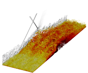
We investigate the interaction of an oblique shock with a flat-plate TBL as illustrated in figure 1. Three LES simulations are performed for this configuration at different Reynolds numbers but otherwise equal flow parameters. The shared parameters, including the geometry of the set-up and the free stream Mach number  $M_{\infty }=2.0$, are also detailed in figure 1. The virtual shock generator is located outside of the computational domain at a fixed distance $g=18.5\delta _{0,i}$ above the wall plane, where $\delta _{0,i}$ denotes the $99\,\%$ velocity-based boundary layer thickness at the inflow plane and remains constant across all cases. The shock generator induces a free stream flow deflection of $\vartheta =10.66^{\circ }$, which is $2^{\circ }$ smaller than the maximum theoretical value for a regular shock reflection at the investigated Mach number (Ben-Dor Reference Ben-Dor2007). The imposed flow deflection results in an oblique shock wave with wave angle $\phi =40.04^{\circ }$, which, in absence of the TBL, would impinge on the wall plane at $x_{imp}$. The channel height to wedge hypotenuse ratio is $g/w=1.16$.
Schematics of the computational domain along with the definition of common parameters to all simulations.

Case-dependent parameters are summarized in table 1, and they are attained by adjusting the free stream dynamic viscosity  $\mu _{\infty }$, see (2.7). We hereafter refer to the low Reynolds STBLI as case $\mathcal {B}_1$, to the moderate Reynolds STBLI as case $\mathcal {B}_2$ and to the high Reynolds STBLI as case $\mathcal {B}_3$.
Case-dependent parameters at the inflow plane and number of cells:  ${\textit {Re}}_{\delta _{0}}=\rho _{\infty }u_{\infty }\delta _{0}/\mu _{\infty }$; ${\textit {Re}}_{\tau }=\bar {\rho }_w u_{\tau } \delta _{0}/\bar {\mu }_w$.

The computational domain is rectangular with dimensions  $[L_x,L_y,L_z]=[45,16.5,4]\delta _{0,i}$ as depicted in figure 1. Non-reflecting boundary conditions based on the Riemann invariants are used at the top and outflow boundaries (Poinsot & Lele Reference Poinsot and Lele1992) while periodicity is imposed in the spanwise direction. The wall is modelled as isothermal at the free stream stagnation temperature, i.e. $T_{wall} = T_0$, and the incident shock and trailing-edge expansion fan are introduced at the top boundary by prescribing conditions based on the Rankine–Hugoniot relations and Prandtl–Meyer theory.
A digital filter technique (Xie & Castro Reference Xie and Castro2008) is used at the inflow plane to prescribe adequate turbulent boundary conditions with well-defined space and time correlations. Details about the implementation of the digital filter technique are provided in Laguarda & Hickel (Reference Laguarda and Hickel2024), and here we consider the filter settings denoted by  $A2$ in their publication. These settings include partitioning the inflow into three distinct zones, each characterized by different target scales, to more accurately represent structures in the inner, overlap and outer layer of the TBL (Veloudis et al. Reference Veloudis, Yang, McGuirk, Page and Spencer2007). The digital filter settings for case $\mathcal {B}_1$, however, omit the overlap-layer zone due to the absence of a distinct logarithmic region at such low Reynolds number ( $0.2\delta _{0}$ corresponds to $y^+\approx 100$ for this case). The prescribed first- and second-order statistical moments at the inflow plane are derived from the DNS data of Pirozzoli & Bernardini (Reference Pirozzoli and Bernardini2011b, Reference Pirozzoli and Bernardini2013) for supersonic TBLs at $M_{\infty } = 2.0$ and comparable friction Reynolds numbers. We also note that the domain size was chosen such that the virtual impingement point $x_{imp}$ is located far downstream of the inflow plane, at a distance $L_{imp}=32\delta _{0,i}$, to ensure proper relaxation of the boundary layer flow to an equilibrium state before it interacts with the incident shock.
A block-structured, piecewise Cartesian grid is constructed in the solution domain with an equal number of grid cells per block but varying grid spacing. At the wall, the spatial resolution properly resolves turbulent structures and the wall shear stress  $\tau _w = \mu _w |\partial u/\partial y|_w$, see table 1. Away from the wall, the grid is coarsened in streamwise and spanwise directions as shown in figure 2. Due to the applied grid stretching in the wall-normal direction (with constant stretching factor), the height of the computational cells increases with wall distance.
Block distribution of the numerical grid for the high Reynolds case  $\mathcal {B}_3$.

The adequacy of the selected grid resolution and domain size was verified through grid- and domain-sensitivity studies involving four distinct grid resolutions and four domain dimensions. The results for case  $\mathcal {B}_2$ are presented in Appendix B and confirm the convergence of the STBLI statistics at the selected grid resolution and domain size. To further support this conclusion, two-point autocorrelation functions of streamwise velocity fluctuations in the homogeneous spanwise direction are reported in Appendix C. These functions are evaluated at multiple locations within the investigated interactions, showing that turbulent fluctuations sufficiently decorrelate over the domain half-width ( $L_z/2$) in all cases.
Computations were initialized with the inviscid shock reflection solution. After an initial transient of  $15$ FTT of the full domain length, all STBLI cases were integrated for over $90$ FTT to properly resolve low-frequency dynamics. Flow statistics were computed by averaging the instantaneous three-dimensional solution in time and spanwise direction, with solution data collected at a sampling rate of $\Delta t\approx 0.02\delta _{0,i}/u_{\infty }$. Additionally, instantaneous three-dimensional snapshots of the interaction region were stored every $\Delta t\approx 0.5\delta _{0,i}/u_{\infty }$ for processing purposes, yielding an ensemble size of $\sim 8200$ snapshots per case.
3. Results
3.1. Incoming TBL
Characterizing the approaching TBL is particularly instructive for the present analysis since Reynolds number effects in STBLI also stem from the differences in the upstream TBL structure at low and high Reynolds number. For this purpose, additional simulations were performed using the same numerical set-up and inflow conditions described in § 2 but in absence of the impinging shock and expansion fan. Statistics and instantaneous three-dimensional snapshots were collected for  $12$ FTT after the initial transient, at the same sampling frequency as in the STBLI simulations.
The low, moderate and high Reynolds undisturbed TBLs are referred to as cases  $\mathcal {T}_1$, $\mathcal {T}_2$ and $\mathcal {T}_3$, respectively. A summary of relevant TBL parameters evaluated at the virtual impingement point $x_{imp}$ is provided in table 2. These parameters are used for scaling purposes in this section and also for the corresponding STBLI cases discussed in § 3.2 and § 3.3.
Undisturbed TBL parameters at the virtual impingement point  $x_{imp}$ without the shock.

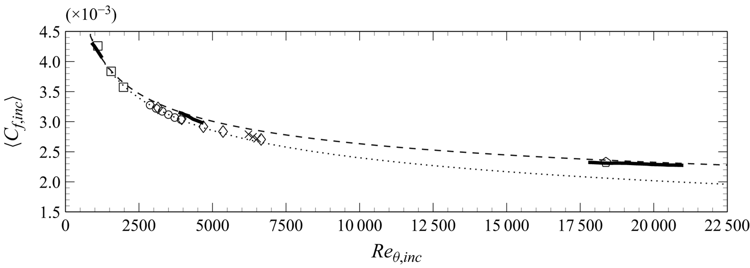
The evolution of the skin-friction coefficient against the momentum-thickness Reynolds number is shown in figure 3. The van Driest II transformation (Van Driest Reference Van Driest1956) has been employed to remove compressibility effects (Shahab et al. Reference Shahab, Lehnasch, Gatski and Comte2011; Hadjadj et al. Reference Hadjadj, Ben-Nasr, Shadloo and Chaudhuri2015). This leads to the equivalent incompressible skin-friction  $\langle C_{f,inc} \rangle$ and incompressible momentum-thickness Reynolds number ${\textit {Re}}_{\theta,inc}$ shown in the figure. Incompressible correlations as well as numerical and experimental data at different conditions are also included in figure 3 for reference (see caption). The present LES results are in very good agreement with the reference data, most notably with the Kármán–Schoenherr correlation and the high Reynolds experimental data of Bross et al. (Reference Bross, Scharnowski and Kähler2021) at $M_{\infty }=2.0$ and ${\textit {Re}}_{\tau }=4680$.
Incompressible skin-friction distribution as a function of  ${\textit {Re}}_{\theta,inc}$. Line legend: (——) present LES data; (- - -) Kármán–Schoenherr (Schoenherr Reference Schoenherr1932); ( $\cdots \cdots$) Smits, Matheson & Joubert (Reference Smits, Matheson and Joubert1983). Symbol legend: ( $\Box$) Simens et al. (Reference Simens, Jiménez, Hoyas and Mizuno2009); ( $\diamondsuit$) Sillero et al. (Reference Sillero, Jiménez, Moser and Malaya2011); ( $\circ$) Pirozzoli & Bernardini (Reference Pirozzoli and Bernardini2011b); ( $\times$) Pasquariello et al. (Reference Pasquariello, Hickel and Adams2017), (
 ) Bross, Scharnowski & Kähler (Reference Bross, Scharnowski and Kähler2021).
Regarding velocity statistics, we first note that the maximum magnitude of the fluctuating Mach number encountered is  $\sqrt {M^{\prime 2}}\approx 0.2$, in agreement with previous compressible studies at similar conditions (Lagha et al. Reference Lagha, Kim, Eldredge and Zhong2011b; Pirozzoli & Bernardini Reference Pirozzoli and Bernardini2011b). As argued by Smits & Dussauge (Reference Smits and Dussauge2006), this (small) value justifies the applicability of Morkovin's hypothesis (Morkovin Reference Morkovin1962) to the simulation data, implying that typical incompressible velocity statistics can be recovered from the present compressible results by simply accounting for mean-property variation effects.
Accordingly, figure 4(a) shows the mean velocity profile for each case following the van Driest transformation, which accounts for mean density variations by scaling the velocity gradient with  $\sqrt {\bar {\rho }/\bar {\rho }_{w}}$ (where $\bar {\rho }_{w}$ is the mean density at the wall, see table 2). This transformation is most effective at collapsing adiabatic or quasiadiabatic TBL data (Trettel & Larsson Reference Trettel and Larsson2016), which is the case for the present LES. Figure 4(a) confirms the collapse of the van Driest-transformed profiles in the inner layer, which exhibit a viscous sublayer with close linear behaviour and an overlap layer in line with the logarithmic law of the wall. For case $\mathcal {T}_3$, see the solid line in figure 4(a), the corresponding (quasi)logarithmic region extends for over a decade of inner-scaled wall distance, up to $y^+\approx 700$, owing to the high Reynolds number of this simulation.
(a) van Driest-transformed mean streamwise velocity profile, and (b) density-scaled Reynolds stresses: (-  ${\cdot }$ - ${\cdot }$) $\mathcal {T}_1$; (- - -) $\mathcal {T}_2$; (——) $\mathcal {T}_3$; ( $\bullet$, red) reference DNS data of Pirozzoli & Bernardini (Reference Pirozzoli and Bernardini2011b, Reference Pirozzoli and Bernardini2013) at $M_{\infty }=2.0$ and ${\textit {Re}}_{\tau }\approx [250,1100,4000]$.
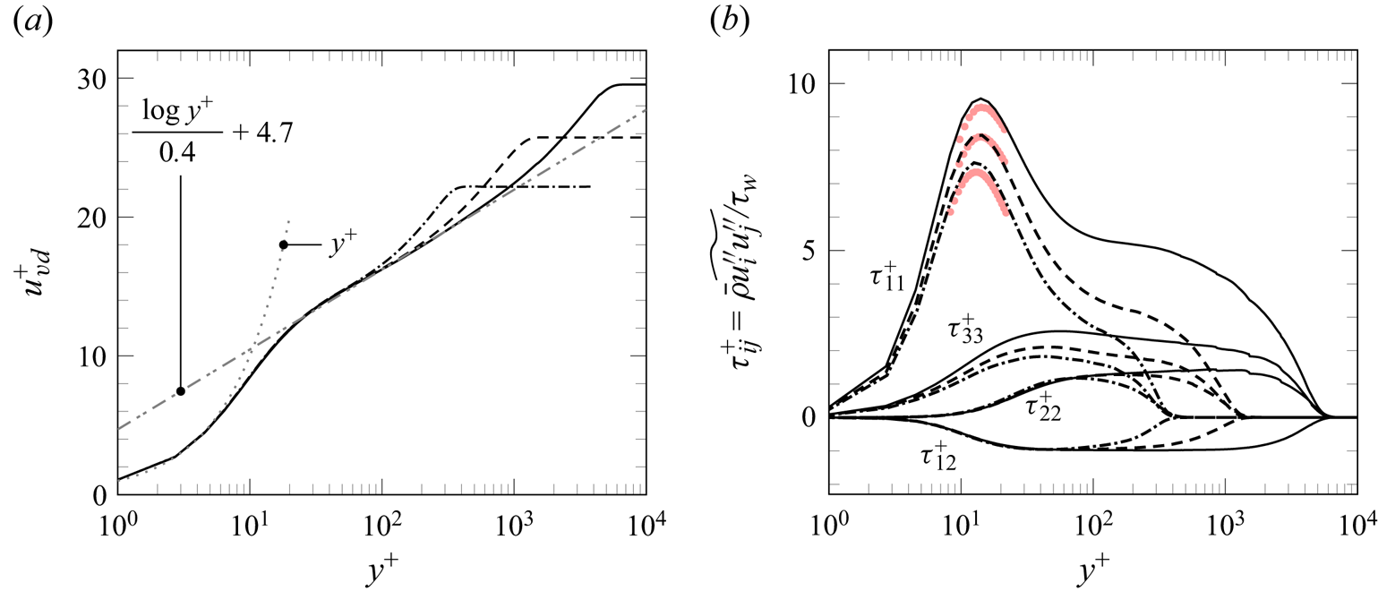
Density-scaled Reynolds stresses are reported in figure 4(b), and they exhibit the expected trend with increasing  $Re_{\tau }$; a noticeable increase in fluctuation intensity for the wall-parallel velocity components. This is attributed to the large-scale coherent motions emerging in the near-logarithmic region at high Reynolds number (Hutchins et al. Reference Hutchins, Nickels, Marusic and Chong2009; Pirozzoli & Bernardini Reference Pirozzoli and Bernardini2013). Such log-layer structures are known to exert a modulating influence on the near-wall cycle, which explains the accompanying increase in peak intensity for the streamwise stress (Hutchins & Marusic Reference Hutchins and Marusic2007b). The good agreement with the reference DNS data of Pirozzoli & Bernardini (Reference Pirozzoli and Bernardini2011b), presented near the streamwise stress peak locations in figure 4(b), confirms that the distinct peak values are very well captured in the present LES.
An important aspect of the TBL in the context of STBLI flows is the size of the underlying turbulent structures, which is addressed by inspecting energy spectra of streamwise velocity fluctuations. Figure 5(a) presents the streamwise spectra in premultiplied form at two different heights above the wall,  $y^+\approx 15$ (grey lines) and $y\approx 0.1\delta _{0}$ (black lines). The former height corresponds to the peak in streamwise velocity fluctuation, while the latter is found in the quasilogarithmic region of the moderate and high Reynolds TBL cases $\mathcal {T}_2$ and $\mathcal {T}_3$. Spectral distributions have been computed using Welch's algorithm with Hanning windows and three segments with $75\,\%$ overlap, in addition to the averaging in spanwise direction and in time.
(a) Premultiplied streamwise spectra of streamwise velocity fluctuations at (grey)  $y^+\approx 15$ and (black) $y\approx 0.1\delta _{0}$, and (b) spanwise spectra of streamwise velocity fluctuations at $y\approx 0.1\delta _{0}$: (- ${\cdot }$ - ${\cdot }$) case $\mathcal {T}_1$; (- - -) case $\mathcal {T}_2$; (——) case $\mathcal {T}_3$.

In the near-wall region ( $y^+\approx 15$), all cases in figure 5(a) show a distinct peak at an outer-scaled wavelength that decreases with increasing Reynolds number. Its inner-scaled value, however, remains constant for all Reynolds numbers at $\lambda ^+\approx 700$. This peak corresponds to the signature of energetic velocity streaks near the wall, which play a key role in the turbulence regeneration cycle (Lagha et al. Reference Lagha, Kim, Eldredge and Zhong2011a). Farther away from the wall, at $y\approx 0.1\delta _{0}$, noticeable differences emerge in the spectra. For case $\mathcal {T}_1$, the most energetic wavelength aligns with that at $y^+\approx 15$, suggesting continued association with near-wall streaks. This association is less evident in case $\mathcal {T}_2$, which exhibits a broader spectral distribution characteristic of moderate Reynolds TBLs (Smits, McKeon & Marusic Reference Smits, McKeon and Marusic2011). The high Reynolds case $\mathcal {T}_3$ presents the broadest range of energetic scales along with a distinct spectral peak at $\lambda _x\approx 5$– $6\delta _{0}$, roughly $30$ times larger than the wavelength associated with near-wall streaks. The presence of these two distinct peaks in the spectra, which closely align with the values reported by Hutchins & Marusic (Reference Hutchins and Marusic2007b) for an incompressible TBL at ${\textit {Re}}_{\tau }\approx 7300$, highlights the clear inner–outer scale separation and the genuinely high Reynolds nature of case $\mathcal {T}_3$.
Spanwise spectra at  $y\approx 0.1\delta _{0}$ are reported in figure 5(b) to provide an estimation of the spanwise spacing of the log-layer structures. All cases show reasonable agreement at high wavelengths, with cases $\mathcal {T}_2$ and $\mathcal {T}_3$ also exhibiting close $\kappa _{z}^{-5/3}$ behaviour in the inertial subrange. Moreover, the spectra exhibit a common peak at $\lambda _z \approx 0.7\delta _{0}$, indicating predominant structures of this width. These observations align with experimental studies at different Reynolds numbers (Hutchins & Marusic Reference Hutchins and Marusic2007a; Bross et al. Reference Bross, Scharnowski and Kähler2021), where the spanwise length scale of log-layer structures has been also found of order $O(\delta _{0})$ and virtually unaffected by Reynolds number.
The present spectral analysis thus reveals that the elongated structures populating the TBL can be up to  $5$–
$5$– $6\delta _{0}$ long and approximately $\sim 0.7\delta _{0}$ wide. To assess the potential modulating influence that they can exert on the STBLI dynamics, figure 6 presents two-dimensional power spectral density (PSD) maps of streamwise velocity fluctuations in the spanwise direction and in time at three wall-normal locations. The corresponding fluctuation signals have been extracted from the STBLI simulations upstream of the interaction, with a $90$ FTT time history that allows for the resolution of potential low-frequency tones that could influence the interaction dynamics. The Strouhal number $St_{\delta _{0}}=f\delta _{0}/u_{\infty }$ is calculated using $\delta _{0}$ (primary ordinate) and $St_{L_{sep}}=fL_{sep}/u_{\infty }$ is calculated using $L_{sep}$ (secondary ordinate), where $L_{sep}$ corresponds to the separation length, which is the distance between the mean separation and reattachment points in the corresponding STBLI. For the estimation of the two-dimensional spectra, the $90$ FTT time intervals have been divided into $10$ overlapping segments along the time axis (with a $65\,\%$ overlap) and windowed with the Hann window function.
Two-dimensional PSD maps of streamwise velocity fluctuations in the homogeneous spanwise direction and in time at three wall-normal locations upstream of the investigated STBLIs. Spectral maps are presented in premultiplied form and normalized by the variance, with blue-filled contours depicting four isocontours from  $0.075$ to $0.3$.

Spectral distributions in figure 6 highlight the decrease in length and time scales of near-wall turbulence as the Reynolds number increases. Figure 6(c i) additionally shows the emergence of an energetic branch at high-wavelengths ( $\lambda _z/\delta _0 > 0.1$) for the high Reynolds case at $y^+\approx 15$, indicating the presence of energetic outer-layer structures influencing the near-wall cycle. Farther away from the wall, at $y\approx 0.1\delta _0$, the spectra exhibit the broadest widening for the high Reynolds case, with spectral energy shifting towards lower frequencies. The energetic fluctuations, however, do not exceed a lower bound of $St_{L_{sep}}\approx 0.1$ (see the left-hand ordinate), which is higher than the typical 0.03–0.06 range reported in the literature for the low-frequency unsteadiness of STBLIs (Clemens & Narayanaswamy Reference Clemens and Narayanaswamy2014). This observation suggests that, in line with many other works in the literature, the dynamics of strong interactions at $St_{L_{sep}}<0.1$ are not directly caused by the passage of incoming long-wavelength structures.
A final observation pertains to the modulating influence of outer-layer structures and bulges on the STBLI flow. Figure 6 indicates that these structures, characterized by energetic spanwise scales of order  $0.1$ to $1\delta _{0}$ in all cases, can contribute to both moderate-frequency ( $St_{L_{sep}}\sim 0.1$– $1$) and high-frequency ( $St_{L_{sep}}\sim 10$) spanwise wrinkling of the separation-shock foot (Muck et al. Reference Muck, Andreopoulos and Dussauge1988; Gross, Little & Fasel Reference Gross, Little and Fasel2022).
3.2. STBLI organization
3.2.1. Instantaneous flow configuration
Instantaneous impressions of the temperature fields are provided in figure 7 to illustrate the resulting STBLI topology. Solid lines indicate instantaneous (yellow) and mean (white) contours of zero streamwise velocity, and show that the adverse pressure gradient imposed by the incident shock is strong enough to cause substantial (mean-)flow separation in all cases. For the higher Reynolds cases, that is, cases  $\mathcal {B}_2$ and $\mathcal {B}_3$, the separation shock emanates from deep within the TBL; for the low Reynolds case $\mathcal {B}_1$, in turn, the compression fan generated at the leading edge of the separated flow region is only coalescing into a shock wave well outside the TBL. This is directly linked to the height and curvature of the sonic line (from which compression waves emanate), which is Reynolds number dependent and dictates the intensity of the separation shock footprint on the surface (Dolling & Murphy Reference Dolling and Murphy1983).
Instantaneous temperature fields: (a) case  $\mathcal {B}_1$; (b) case $\mathcal {B}_2$; (c) case $\mathcal {B}_3$. Solid lines indicate instantaneous (yellow) and mean (white) isocontours of zero streamwise velocity, and $\blacktriangle$ indicates mean separation (S) and reattachment (R) locations.

At the separation shock foot, the flow is strongly decelerated and starts to detach. Turbulent structures from the upstream TBL are seeded into the free shear layer, and grow in size as they move away from the wall. The upper limit of the separation bubble is eventually established as a result of the interaction between the detached shear layer and the incident-transmitted shock, which turns the flow back towards the surface and initiates the reattachment process. All STBLI cases exhibit a very mild concave streamline curvature near reattachment, which translates into a weak compression fan instead of a coalesced reattachment shock. We also note that the intersection between the incident and the separation shock occurs approximately  $2.5\delta _{0}$ above the wall in all cases.
The organization of the investigated STBLI flows is further examined by employing the swirling strength criterion  $\lambda _{ci}$ to visualize instantaneous turbulent structures. This criterion is based on local spiralling motion, which in the vicinity of vortex cores translates into a real eigenvalue $\lambda _{r}$ plus a pair of complex conjugate eigenvalues $\lambda _{cr}\pm i\lambda _{ci}$ of the velocity gradient tensor (Zhou et al. Reference Zhou, Adrian, Balachandar and Kendall1999). In figure 8, coherent vortical structures in the investigated STBLIs are visualized by plotting an isosurface of the magnitude of the imaginary part of the complex conjugate eigenvalue $\lambda _{ci}$. In this figure, turbulent structures are also coloured by the local streamwise velocity, and a numerical schlieren visualization is included in the background of each rendering for reference. The Reynolds number increases from figure 8(a) to figure 8(c).
Instantaneous vortical structures visualized with the  $\lambda _{ci}$ criterion and coloured by the local streamwise velocity: (a) case $\mathcal {B}_1$ ( $|\lambda _{ci}|\delta _{0}/u_{\infty }=2.2$); (b) case $\mathcal {B}_2$ ( $|\lambda _{ci}|\delta _{0}/u_{\infty }=3.8$); (c) case $\mathcal {B}_3$ ( $|\lambda _{ci}|\delta _{0}/u_{\infty }=5.6$). A numerical schlieren is shown in the background slice for each case, and the streamwise velocity colour bar applies to all renders.

Figure 8 reveals clear differences in terms of size and organization of turbulent structures at low and high Reynolds number. Starting from the upstream TBL, structures resembling hairpin vortices can be observed for the low Reynolds case  $\mathcal {B}_1$, see figure 8(a). The higher Reynolds cases $\mathcal {B}_2$ and $\mathcal {B}_3$, in contrast, exhibit structures of much smaller size that do not conform to the canonical hairpin vortex. This is in agreement with the observations made by Pirozzoli & Bernardini (Reference Pirozzoli and Bernardini2011b) on a $M_{\infty }=2.0$ TBL flow at ${\textit {Re}}_{\tau }\approx 1100$.
At the leading edge of the interaction, where incoming turbulence is compressed and the shear layer detaches from the wall, spanwise variations become more pronounced at high Reynolds number, see figure 8(b,c). Based on the colour of the structures in the detaching shear layer, which indicates the magnitude of the local streamwise velocity, such variations are associated with alternating regions of low- and high-momentum fluid. Furthermore, within and above the high-speed streaks, larger vortical structures emerge in the detached shear layer as it moves away from the wall. These structures then break at the bubble apex, where the overall turbulence intensity is reduced. Past the interaction region, the boundary layer has clearly thickened and all cases exhibit more turbulent structures in the outer region compared with the upstream (undisturbed) TBL.
The background schlieren visualizations emphasize the origin of the separation shock deep within the TBL at high Reynolds number, as seen when comparing figures 8(a) and 8(c). Furthermore, the schlieren visualization in figure 8(b) captures the precise instant when the separation-shock front for the moderate Reynolds case  $\mathcal {B}_2$ is instantaneously deformed by the passage of outer-layer bulges. These structures, of order $\delta _{0}$ in span, contribute to the wrinkling of the separation-shock foot at both moderate and high frequencies, as discussed in § 3.1.
We have emphasized above that, despite the shift towards lower energetic frequencies, the energetic frequency scales of the incoming turbulence for case  $\mathcal {B}_3$ remain too high to significantly impact the low-frequency dynamics of STBLI. However, these structures, associated with larger streamwise wavelengths, still play a crucial role in modulating the flow organization. This is illustrated in figure 9, which shows instantaneous streamwise velocity fluctuations for case $\mathcal {B}_3$ at the same time instance as in figure 8(c).
Instantaneous streamwise velocity fluctuations for case  $\mathcal {B}_3$ at the same time instance as figure 8(c). Isosurfaces in (a) correspond to $u^{\prime }/u_{\infty }=-0.12$ (blue) and $u^{\prime }/u_{\infty }=0.12$ (red), and panels (b–g) illustrate streamwise-normal cuts of (a) at $(x-x_{imp})/\delta _{0}=\{-8.4,-5.6,-4.2,-2,1,5\}$, respectively. A numerical schlieren visualization is shown in the background slice of (a) for reference while solid lines in (b–g) indicate the instantaneous isocontour of zero streamwise velocity (yellow) and pressure gradient $|\boldsymbol {\nabla } p|\delta _{0}/p_{\infty }=4$ (grey).

Three-dimensional isosurfaces of positive (red) and negative (blue) streamwise velocity fluctuations are shown in figure 9(a), while figure 9(b–g) depict two-dimensional contours on  $yz$ slices at $(x-x_{imp})/\delta _{0}=\{-8.4,-5.6,-4.2,-2,1,5\}$. These visualizations reveal clear correlations between spanwise variations of the separation shock (grey lines) and the edge of the reverse-flow bubble (yellow lines) with alternating regions of low- and high-momentum fluid in the incoming TBL. At the leading edge of the interaction, they strongly modulate the separation-shock foot, see figure 9(c), where the passage of high-speed fluid brings the shock foot closer to the wall and also delays separation right at the surface. Moreover, as these velocity structures traverse the interaction, they reorganize and progressively exhibit much stronger spatial coherence. This is evident when comparing figure 9(b), representing the upstream TBL, with figure 9(g), corresponding to a location downstream of the interaction region. Spanwise autocorrelation functions at these two locations (reported in Appendix B) clearly highlight this increase in coherence, which is observed across all investigated Reynolds numbers.
Previous works have identified the resulting large-scale velocity structures beyond reattachment as the imprint of Görtler-like vortices in the interaction region (Priebe et al. Reference Priebe, Tu, Rowley and Martín2016; Pasquariello et al. Reference Pasquariello, Hickel and Adams2017; Hu et al. Reference Hu, Hickel and van Oudheusden2021). While these studies also argue that such structures could play a pivotal role in driving the low-frequency unsteadiness of STBLIs, their actual relevance remains unclear. We attempted to extract any large-scale vortex from the turbulent background by filtering the three-dimensional snapshot data following the approach of Pasquariello et al. (Reference Pasquariello, Hickel and Adams2017). However, the large-scale circulation is so weak compared with the small-scale turbulence in the present interactions that it was not possible to discern Görtler-like vortices in the filtered instantaneous snapshots. Their visualization is, however, possible with modal decomposition techniques applied to the full time series, as will be discussed in § 3.3.3.
3.2.2. Characteristics of the reverse-flow region
The spatial distributions of the average skin-friction coefficient, see figure 10(a), exhibit a large and connected separation region characteristic of strong interactions. The figure also shows that the location of the global minimum in  $\langle C_f \rangle$ is not affected by the Reynolds number and occurs approximately $1\delta _{0}$ upstream of the inviscid impingement point $x_{imp}$. The overall skin-friction distribution within the reverse-flow region, on the other hand, is noticeably different at low and high Reynolds number. The low Reynolds case $\mathcal {B}_1$, indicated with a dash–dotted line in figure 10(a), exhibits a $W$-shaped distribution characteristic of low Reynolds interactions (Priebe, Wu & Martin Reference Priebe, Wu and Martin2009; Aubard, Gloerfelt & Robinet Reference Aubard, Gloerfelt and Robinet2013; Pasquariello et al. Reference Pasquariello, Grilli, Hickel and Adams2014), with a second negative peak right after separation. Conversely, the higher Reynolds cases exhibit a skin-friction plateau in the first half of the separation bubble that precedes the global minimum on the second half.
(a) Time- and spanwise-averaged skin-friction evolution, and (b) probability of reverse-flow: (-  ${\cdot }$ - ${\cdot }$) case $\mathcal {B}_1$; (- - -) case $\mathcal {B}_2$; (——) case $\mathcal {B}_3$. Separated regions in (a) are shaded in red and the grey lines denote the corresponding skin-friction distribution for the undisturbed TBL. Distributions in (b) denote the probability of reverse-flow at the wall (black) and its maximum value in the wall-normal direction (blue).

Despite the aforementioned differences, the separation length  $L_{sep}$, i.e. the distance between mean separation and reattachment points, does not appear to change noticeably in the investigated Reynolds number range, see also table 3. This finding is in agreement with the experimental work of Souverein et al. (Reference Souverein, Dupont, Debieve, Dussauge, van Oudheusden and Scarano2010) involving interactions at ${\textit {Re}}_{\theta }\approx \{5000, 50\,000\}$ and the comparative numerical study of Morgan et al. (Reference Morgan, Duraisamy, Nguyen, Kawai and Lele2013) over the range ${\textit {Re}}_{\theta }=[1500, 4800]$, where $L_{sep}$ was also found insensitive to the Reynolds number.
Topological properties of the interaction region.

Figure 10(a) also includes the skin-friction distribution of the corresponding undisturbed TBLs (grey lines) in order to better appreciate the upstream influence of the STBLI flow. Inspired by Settles et al. (Reference Settles, Bogdonoff and Vas1976), we define the upstream influence parameter  $\Delta x_{ui}=x_{imp}-x_{ui}$ for impinging STBLIs as the distance between the inviscid impingement point $x_{imp}$ and the streamwise location where the skin-friction falls by $1\,\%$ with respect to the undisturbed TBL distribution, denoted by $x_{ui}$. The resulting values for this parameter are also reported in table 3, and they confirm the Reynolds number dependency of the upstream influence that was previously observed in compression ramp flows, i.e. a reduced upstream influence with increasing ${\textit {Re}}_{\tau }$. We find that the logarithmic fit $\Delta x_{ui}/\delta _{0}=-0.357\ln {{\textit {Re}}_{\tau }}+9.689$ approximates the present data with an $R^{2}$ value of $0.995$.
A final remark on figure 10(a) concerns the skin-friction distribution downstream of the interaction. As observed, all curves overshoot the corresponding values of the undisturbed TBLs beyond the reattachment point. This is due to the presence of the expansion fan that originates at the trailing edge of the (virtual) shock generator.
The probability of reverse-flow  $\chi$ is shown in figure 10(b) to further illustrate Reynolds number effects in the shock-induced flow separation. Black lines indicate the probability at the wall, i.e. the fraction of the total time when $C_f<0$, and blue lines consider the maximum value in the wall-normal direction, i.e. the fraction of the total time when $u<0$ at any point above the wall.
Initially, both probability distributions overlap for the lower Reynolds cases  $\mathcal {B}_1$ and $\mathcal {B}_2$, see figure 10(b), until $\chi \approx 0.60$ and $0.45$, respectively. This overlap ends with a local peak in $\chi$ at the wall that reveals the occurrence of partial flow reattachment near the leading edge of the interaction. Interestingly, the location of the local peak for case $\mathcal {B}_1$, found at $(x-x_{imp})/\delta _{0}\approx -5.6$, coincides with the local minimum in skin-friction near separation in figure 10(a). This correspondence suggests that the characteristic $W$-shaped distribution of $\langle C_f \rangle$ in low Reynolds interactions is a result of partial flow reattachment right after separation.
For the high Reynolds case  $\mathcal {B}_3$, both probability distributions in figure 10(b) only overlap until $\chi \approx 0.25$. Moreover, all cases exhibit a maximum in reverse-flow probability at $x-x_{imp}=-\delta _{0}$, where $\chi$ is almost unity for cases $\mathcal {B}_2$ and $\mathcal {B}_3$ when considering the maximum value in the wall-normal direction (see the corresponding blue lines). The location of this peak is also associated with a negative peak in $\langle C_f \rangle$, as shown in figure 10(a), in this case representing the global minimum.
The effect of Reynolds number on the recirculation bubble topology is further analysed using a set of topology parameters defined in figure 11(a) and reported in table 3. These parameters include the aspect ratio of the bubble, represented by its height  $h_{rev}$ normalized by $L_{sep}$, and the bubble area $A_{rev}$, which corresponds to its volume per unit span. The latter is normalized by the area of the triangle formed by the separation point, bubble apex and reattachment point locations to highlight the degree of compliance with a perfect triangular shape (with area $h_{rev}L_{sep}/2$).
(a) Relevant definitions concerning the interaction topology, and (b) close-up view of the recirculation region. Dividing streamlines are marked with solid black lines in (b), and blue lines are streamlines passing through  $y/\delta _{0}=\{0.05, 0.3\}$ at $x-x_{imp}=-7\delta _{0}$. Dotted grey lines indicate isocontours of reverse-flow probability ( $\chi =0.01$ and $0.8$), and dashed magenta lines show the free stream flow deflection.

For the higher-Reynolds cases  $\mathcal {B}_2$ and $\mathcal {B}_3$, the normalized $A_{rev}$ is very close to unity, see table 3, which indicates that the corresponding bubbles closely resemble triangles. Conversely, the recirculation bubble for the low Reynolds case $\mathcal {B}_1$ has a smaller normalized $A_{rev}$ of $0.78$. A close-up view of the different recirculation regions in figure 11(b) reveals that the reversed flow is initially confined to the wall for this case, over a distance of approximately $2\delta _{0}$ before the shear layer moves away from the wall. This is consistent with the presence of a compression fan instead of a coalesced separation shock at the leading edge of the interaction, and explains the greater deviation of the bubble shape from a perfect triangle.
Additionally, each panel in figure 11(b) includes the dividing streamline (black line) and two other streamlines above the separation region (blue lines). For the low Reynolds case  $\mathcal {B}_1$, these streamlines exhibit a much larger curvature radius around the leading edge of the separation bubble. The postshock flow deflection $\vartheta _{sep}$ is slightly larger than $12\,^{\circ }$ in all cases and essentially independent of the Reynolds number. This deflection is also indicated in figure 11(b) and reported in table 3, along with the corresponding theoretical shock angle $\phi _{sep}$.
Furthermore, table 3 provides additional parameters that assess the symmetry between the leading and trailing portions of the bubble. These parameters include the corresponding distance between the separation point and the streamwise location of the bubble apex, denoted  $L_u$ following the nomenclature used by Giepman (Reference Giepman2016) for laminar and transitional interactions (see also figure 11a). The corresponding volume of the bubble above this segment, $A_u$, is also reported and highlighted with a red shade in figure 11. Interestingly, both symmetry parameters reveal that the separation bubble for case $\mathcal {B}_2$ exhibits the highest degree of symmetry in shape, with $L_u=0.56L_{sep}$ and $A_u=0.53A_{rev}$. This symmetry is visually evident upon inspecting figure 11(b). The reverse-flow probability within the bubble, however, is clearly asymmetric in all cases, as indicated by the $\chi =0.8$ isocontour.
The isocontour of  $\chi =0.01$ is also included in figure 11(b) to illustrate the extent of the instantaneous reverse-flow. According to Simpson's terminology for TBL separation, $\chi =0.01$ marks the condition for incipient separation (Simpson et al. Reference Simpson1989). This isocontour appears as an essentially straight line at the leading edge of the bubble in all cases, see figure 11(b), and closely follows the postshock deflection of the outer flow. Notably, the maximum height above the wall of the $\chi =0.01$ isocontour is approximately $0.9\delta _{0}$, which is two to three times higher than the mean bubble height $h_{rev}$. Moreover, at the trailing edge of the bubble, the contour line is curved and eventually meets the wall approximately $2\delta _{0}$ downstream of the reattachment point. We use the streamwise distance over which the reverse-flow probability is higher than $\chi =0.01$ to define the reverse-flow-based length scale $L_{\chi }$. This parameter could serve as an alternative to $L_{sep}$ in cases involving weakly separated STBLIs with partitioned bubbles. For the present strong interactions, $L_{\chi }$ remains approximately $11\delta _{0}$ and shows little sensitivity to the Reynolds number (see table 3).
3.2.3. Mean and fluctuating wall pressure
After discussing the corresponding differences in recirculation-bubble topology, we now consider the impact of Reynolds number on wall-pressure characteristics of STBLIs. Figure 12(a) shows the mean wall-pressure distribution for the investigated interactions, all exhibiting the typical features of strong STBLIs with substantial flow separation (Matheis & Hickel Reference Matheis and Hickel2015; Pasquariello et al. Reference Pasquariello, Hickel and Adams2017). Characteristic inflection points associated with separation, the onset of reattachment and the reattachment compression are discernible on each curve (Délery, Marvin & Reshotko Reference Délery, Marvin and Reshotko1986). The low Reynolds case  $\mathcal {B}_1$, however, presents a more gradual pressure rise at the leading edge of the interaction as a result of the diffuse separation-shock foot, while the higher Reynolds cases $\mathcal {B}_2$ and $\mathcal {B}_3$ exhibit a sharper pressure increase. The pressure plateau is not fully established in any of the cases, and its magnitude, in close agreement with the predictions by Zukoski (Reference Zukoski1967), appears insensitive to the Reynolds number.
Time- and spanwise-averaged (a) wall pressure, and (b) wall-pressure fluctuation intensity. For the line legend, see caption of figure 10. Mean separation and reattachment points are indicated with a marker ( $\bullet$), and the plateau pressure computed according to the empirical formula by Zukoski (Reference Zukoski1967) is also shown in (a).

The corresponding wall-pressure fluctuation intensities are presented in figure 12(b). In contrast to the low Reynolds case  $\mathcal {B}_1$, which lacks a discernible peak at the leading edge of the interaction, indicative of attenuated wall-pressure intermittency (Priebe et al. Reference Priebe, Wu and Martin2009), distinct peaks are clearly visible for the higher Reynolds interactions due to the stronger separation-shock footprint on the surface. Notably, the peak intensity is almost twice as large for case $\mathcal {B}_3$ compared with $\mathcal {B}_2$. Additionally, case $\mathcal {B}_3$ exhibits the highest wall-pressure fluctuation intensities throughout the interaction, while the lowest values are observed for case $\mathcal {B}_2$. This observation further evidences the non-monotonic effect of Reynolds number on the interaction dynamics. Despite varying magnitudes, the curves in figure 12(b) share common features in good qualitative agreement with previous works on impinging STBLIs (e.g. Dupont et al. Reference Dupont, Haddad and Debieve2006; Pasquariello et al. Reference Pasquariello, Hickel and Adams2017). Specifically, all distributions show an increased level of fluctuation intensity postseparation, attributed to the flapping motion of the shear layer (Dupont et al. Reference Dupont, Haddad and Debieve2006). This is followed by a slight drop in pressure fluctuation intensity within the separated region before rising again due to the reattaching shear layer vortices.
Moreover, the wall-pressure statistics in figure 12 indicate that mean separation occurs downstream of the excursion domain of the separation shock (i.e. beyond the pressure fluctuation intensity peak in figure 12b) for the interactions at higher Reynolds number. We attribute this to the moderate incident-shock strength in the investigated STBLIs, which results in a deeper penetration of the high-momentum flow into the interaction region before the formation of the separation bubble.
3.2.4. Reynolds stresses
The effect of Reynolds number on second-order velocity statistics is analysed next. Figure 13 shows contours of the Favre-averaged streamwise Reynolds stress  $\tau _{11}=\widetilde {u^{''}u^{''}}$. Qualitatively, all cases bear similarities in terms of the location of increased fluctuation intensity, which is mainly confined to the shear layer at the leading edge of the separated region. This is in good agreement with previous works (Dupont et al. Reference Dupont, Piponniau, Sidorenko and Debiève2007; Pirozzoli et al. Reference Pirozzoli, Larsson, Nichols, Bernardini, Morgan and Lele2010; Pasquariello et al. Reference Pasquariello, Hickel and Adams2017). Additionally, $\tau _{11}$ is highly damped by the strong convex curvature at the bubble apex in all cases. As pointed out by Sandham (Reference Sandham2016), such curvature effects are strongest for this stress component.
Time- and spanwise-averaged streamwise Reynolds stress  $\tau _{11}=\widetilde {u^{''}u^{''}}$ for (a) case $\mathcal {B}_1$, (b) case $\mathcal {B}_2$ and (c) case $\mathcal {B}_3$. Solid line colour legend: (yellow) $\langle u \rangle = 0$; (grey) dividing streamline; (purple) $\langle M \rangle = 1$; (black) $95\,\%$ of $\max (\tau _{11})$. Green dashed lines mark selected streamlines, and $\square$ and $\triangle$ indicate the locations of $\max (\tau _{11})$ and max $(\mathcal {P}_{11})$, respectively.

One notable observation concerns the disparity in the location of maximum  $\tau _{11}$ across the different cases, as indicated by the $\square$ symbols in figure 13. It is evident that in figure 13(a,b), for the lower-Reynolds cases $\mathcal {B}_1$ and $\mathcal {B}_2$, this point is found near the separation-shock foot, where the production of $\tau _{11}$, i.e. $\mathcal {P}_{11}$, is highest. This point is indicated with a $\triangle$ symbol. Conversely, for the high Reynolds case $\mathcal {B}_3$ in figure 13(c), the streamwise stress distinctly peaks within the detached shear layer, which is no longer correlated with $\text {max}(\mathcal {P}_{11})$ (see also the isocontours of $95\,\%$ of $\max (\tau _{11})$ shown as black solid lines).
Previous numerical studies, such as Fang et al. (Reference Fang, Zheltovodov, Yao, Moulinec and Emerson2020) and the recent work of Kang & Lee (Reference Kang and Lee2024), which have examined turbulence amplification across canonical STBLIs, consistently identified peak locations of  $\tau _{11}$ and turbulence kinetic energy beneath the separation-shock foot and near the point of maximum stress production. While these findings are consistent with our observations in the lower-Reynolds cases, the observed disparity in stress peak locations for case $\mathcal {B}_3$ suggests that the widely accepted $\tau _{11}$ amplification mechanism proposed in the literature, which is associated with the deceleration of the mean flow and the near-wall cycle of the TBL, may not be the primary source of stress at high Reynolds number.
To clarify this, we analyse the corresponding transport budgets along two mean-flow streamlines crossing the interaction. The first streamline, labelled  $s_{a}$ in figure 13, intersects the point of $\text {max}(\mathcal {P}_{11})$ in all cases, which is consistently located in the near-wall region beneath the separation-shock foot. As shown in the inset panels of figure 13(a,b), this point is indeed in close proximity to the point of maximum $\tau _{11}$ for the lower-Reynolds cases $\mathcal {B}_1$ and $\mathcal {B}_2$. The second selected streamline, labelled as $s_b$, cuts through the shear layer as shown in figure 13. Notably, this intersection highlights the misalignment between the mean flow and the track of maximum stress in the detached shear layer. For the high Reynolds case $\mathcal {B}_3$, $s_b$ is selected such that it intersects the location of maximum $\tau _{11}$ over the interaction (i.e. the $\square$ symbol in figure 13c).
The distributions of the  $\tau _{11}$ transport budgets along the above-mentioned streamlines are depicted in figure 14. The various terms involved in the transport equation for the Favre-averaged Reynolds stresses are detailed in Appendix D, and they include production, $\mathcal {P}$, viscous diffusion, $\mathcal {D}^{\nu }$, turbulent convection, $\mathcal {D}^{t}$, pressure transport, $\mathcal {D}^{p}$, pressure–strain correlation, $\varPi$, turbulent mass flux, $\mathcal {M}$, and dissipation, $\epsilon$. The convective term of the material derivative is evaluated as it appears on the left-hand side of (D1) (with the sign unchanged) so that it serves as an indication of net $\tau _{11}$ gain. For clarity, two-dimensional contours of the most relevant terms are also shown in figure 15, and they should be considered alongside the discussion of figure 14.
Transport budgets for  $\tau _{11}$ along (a,c,e) streamline $s_a$, and (b,d,f) streamline $s_{b}$: (a,b) case $\mathcal {B}_1$; (c,d) case $\mathcal {B}_2$; (e,f) case $\mathcal {B}_3$. Symbol legend: production $\mathcal {P}_{11}$ ( $\blacksquare$, black); viscous diffusion $\mathcal {D}^{\nu }_{11}/\bar {\rho }$ ( $\blacktriangleleft$, teal); turbulent convection $\mathcal {D}^{t}_{11}/\bar {\rho }$ ( $\blacktriangle$, green); pressure transport $\mathcal {D}^{p}_{11}/\bar {\rho }$ ( $\blacktriangleright$, orange); pressure–strain correlation $\varPi _{11}$ (
 , blue); turbulent mass flux $\mathcal {M}_{11}$ ( $\times$, yellow); dissipation $\epsilon _{11}$ ( $\blacklozenge$, grey); convection $\tilde {u}_k \partial _k \tau _{11}$ ( $\bullet$, magenta). For reference, the evolution of $\tau _{11}$ (normalized by $u^2_{\infty }$) is also indicated with a solid red line.

Contours of selected  $\tau _{11}$ transport budgets: (a–c) production $\mathcal {P}_{11}$; (d–f) pressure–strain correlation $\varPi _{11}$; (g–i) pressure transport $\mathcal {D}^{p}_{11}$; (j–l) turbulent convection $\mathcal {D}^{t}_{11}$. Panels (a,d,g,j), (b,e,h,k) and (c,f,i,l) correspond to cases $\mathcal{B}_1, \mathcal{B}_2$ and $\mathcal{B}_3$, respectively, as indicated at top of panels (a,d,g,j). Contour levels are shown from $-0.05 u_{\infty }^3/\delta _{0}$ (dark blue) to $0.05 u_{\infty }^3/\delta _{0}$ (dark red).

We consider first the corresponding budget distributions along  $s_{a}$, which are depicted on figure 14(a,c,e). It is clear that the magnitude of the production term at the separation-shock foot is largest for the high Reynolds case $\mathcal {B}_3$ in figure 14(e). However, the amplification of $\mathcal {P}_{11}$ with respect to that of the undisturbed TBL is only $1.06$ , which indicates a minor impact of the mean-flow deceleration in the near-wall production at high Reynolds number. For the other cases, the amplification of this term is much larger; $1.58$ for case $\mathcal {B}_2$ in figure 14(c), and $2.44$ for case $\mathcal {B}_1$ in figure 14(a). In addition, the fact that $\mathcal {P}_{11}$ for case $\mathcal {B}_3$ exhibits a progressive increase in the upstream boundary layer is simply a result of the selected streamline deviating away from the wall, from $y^+\approx 6$ on the left-hand side of of figure 14(e) to $y^+\approx 10$ at the peak production. This deviation naturally alters the value of the production term as well as other terms like turbulent transport $\mathcal {D}^{t}_{11}$, which changes from a positive to a negative value. Thus, an indication of the STBLI onset is where previously inactive terms in the undisturbed TBL, like convection or pressure transport, become active.
Figure 14(c,e) reveal that the convection term, which indicates net  $\tau _{11}$ gain, is correlated with the initial amplification of the pressure transport term for the higher Reynolds cases $\mathcal {B}_2$ and $\mathcal {B}_3$. This is caused by the stronger footprint of the separation-shock dynamics at the wall, which leads to large negative values of the pressure $-$streamwise-velocity correlation for these cases and consequently a sharp rate of change in streamwise direction. The streamwise extent of increased pressure transport $\mathcal {D}^{p}_{11}$, including both positive and negative values, thus reflects the streamwise excursion range of the separation shock. For the low Reynolds case $\mathcal {B}_1$, in contrast, the more gradual compression and thus weaker footprint of the separation-shock dynamics at the wall result in negligible pressure-transport contributions. Here, the increase in $\tau _{11}$ is solely attributed to the amplification of $\mathcal {P}_{11}$ driven by the deceleration of the mean flow, see figure 14(a). This corresponds to the amplification mechanism previously reported in the literature (Fang et al. Reference Fang, Zheltovodov, Yao, Moulinec and Emerson2020), which this analysis demonstrates to be predominant only at low Reynolds numbers. Furthermore, the increase in pressure–strain correlation $\varPi _{11}$ eventually brings the amplification of $\tau _{11}$ to an end in all cases. The pressure–strain correlation is responsible for the redistribution of energy from the longitudinal stress $\tau _{11}$ towards the transverse stresses $\tau _{22}$ and $\tau _{33}$ (and indirectly to the shear stress $\tau _{12}$) which exhibit large positive values of $\varPi _{ij}$ at the separation shock foot (not shown here).
The role of pressure transport on the amplification of  $\tau _{11}$ at high Reynolds number is further highlighted in the budget distributions along the streamline $s_{b}$, which are shown on figure 14(b,d,f) for all cases. The level of $\mathcal {P}_{11}$ in the upstream TBL is much lower along this streamline, as expected away from the wall. For case $\mathcal {B}_{1}$, the progressive amplification of the production term together with increased turbulent convection $\mathcal {D}^{t}_{11}$ lead to a net gain in streamwise stress, see figure 14(b). A similar scenario is observed for case $\mathcal {B}_{2}$ in figure 14(d), with an additional contribution of pressure transport, albeit very moderate, at the leading edge of the interaction. The role of pressure transport, however, is much more significant for case $\mathcal {B}_{3}$ in figure 14(f). As shown, the evolution of the convection term at the leading edge of the interaction is highly correlated with the pressure-transport budget, especially its initial steep rise and peak value (occurring at $y^+\approx 350$). This results in the largest rate of change of $\tau _{11}$, which also contributes to the rapid amplification of $\mathcal {P}_{11}$. Even though the magnitude of the production term is much lower than the global production peak observed in the near-wall region (see figure 14e), it undergoes a much larger amplification from the free stream value along this streamline. Once the pressure-transport contribution becomes negative, the increased production (also affected by the mean-flow deceleration) and turbulent diffusion terms still enable a net gain in $\tau _{11}$ for over half a boundary layer thickness in the streamwise direction, eventually leading to the global peak stress along the detached shear layer.
The present analysis thus demonstrates that the maximum amplification of  $\tau _{11}$ at high Reynolds number is not linked to the near-wall cycle of the approaching TBL and is not so much influenced by the mean-flow deceleration at the leading edge of the interaction. Instead, it is largely driven by the unsteadiness of the (sharp) separation shock, which has a much stronger footprint close to the wall. As a result of the large pressure–streamwise-velocity correlation in the shock-excursion domain, the pressure-transport term acts as an important source of stress that results in the global $\tau _{11}$ peak being located away from the wall and within the detached shear layer. The contours of $\tau _{11}$ production, pressure–strain, pressure-transport and turbulent convection shown at the leading edge of the interaction in figure 15 further illustrate the effect of Reynolds number on the budget terms. In particular, figure 15(g–i) show the $\tau _{11}$ pressure-transport budget $\mathcal {D}^{p}_{11}$, where visible differences in the separation-shock foot region are observed.
For the sake of conciseness, we do not extend the discussion to the other Reynolds stresses, since no apparent Reynolds number dependency was observed in their corresponding amplification. The only other notable difference observed with previous literature is the location of maximum spanwise Reynolds stress  $\tau _{33}=\widetilde {w^{''}w^{''}}$, which is found within the first half of the detached shear layer in the present simulations. This finding is not aligned with the LES results of Pasquariello et al. (Reference Pasquariello, Hickel and Adams2017), where the $\tau _{33}$ peak appears approximately $3\delta _{0}$ downstream of the reattachment location and very close to the wall. We observe a moderate $\tau _{33}$ increase at the same location in our LES data, but the stress intensity is substantially lower than in the majority of the shear layer. Pasquariello et al. (Reference Pasquariello, Hickel and Adams2017) attribute the increased fluctuation to the presence of Görtler-like vortices resulting from the concave streamline curvature at reattachment. While this curvature is rather mild in the present STBLIs, which involve a weaker incident shock than that of Pasquariello et al. (Reference Pasquariello, Hickel and Adams2017), it remains above the critical Görtler number. The observed reorganization of velocity fluctuations across all interactions is also consistent with the presence of streamwise-aligned vortices, see § 3.2.1, but their apparently limited impact on $\tau _{33}$, in line with the observed lower vortex strength, perhaps suggests a less pivotal role in the low-frequency dynamics in our cases.
3.3. STBLI dynamics
In order to assess Reynolds number effects in the dynamics of the investigated STBLIs, we analyse temporal spectra of wall-pressure data, separation-shock location and bubble-volume variations. The most energetic frequencies are then linked to global flow phenomena via dynamic-mode decomposition (DMD) (Schmid Reference Schmid2010) of the LES data. In previous impinging STBLI studies, such modal analysis technique was commonly applied to two-dimensional datasets, often resulting from spanwise averaging (e.g. Grilli et al. Reference Grilli, Schmid, Hickel and Adams2012; Nichols et al. Reference Nichols, Larsson, Bernardini and Pirozzoli2017; Pasquariello et al. Reference Pasquariello, Hickel and Adams2017). Here, we instead employ a full three-dimensional dataset that includes the instantaneous streamwise velocity, pressure and streamwise vorticity fields. In addition, we use the sparsity-promoting variant of the DMD algorithm (known as SPDMD) (Jovanović, Schmid & Nichols Reference Jovanović, Schmid and Nichols2014) to seek a low-rank representation of the most relevant dynamics for each of the investigated Reynolds numbers.
3.3.1. Wall pressure
Figure 16 shows the premultiplied PSD map of the wall pressure for each of the investigated interactions. The corresponding signals were obtained from wall-pressure taps equispaced in the streamwise direction along the domain centreline and sampled at a frequency  $f_s \approx 37u_{\infty }/\delta _{0}$. Spectra have been estimated using Welch's algorithm, with Hanning windows and $10$ segments with $65\,\%$ overlap. The segment length exceeds $100 L_{sep}/u_{\infty }$ in all cases.
Frequency-weighted and normalized PSD map of wall pressure at the centreline: (a) case  $\mathcal {B}_1$; (b) case $\mathcal {B}_2$; (c) case $\mathcal {B}_3$. Dashed lines indicate mean separation $(S)$ and reattachment $(R)$ locations for each case. Contour levels range from zero (white) to $0.3$ (black).

The wall-pressure PSD maps in figure 16 illustrate one of the most prominent features of STBLIs: the shifting of the frequency of the most energetic fluctuations to much lower values. Consistent with previous works, the separation shock exhibits broadband low-frequency dynamics at a separation-length-based Strouhal number  $0.01\lesssim St_{L_{sep}}\lesssim 0.1$. The spatial extent associated with these low-frequency dynamics, indicative of the streamwise excursion domain of the separation shock, is approximately $\delta _{0}$ for the higher-Reynolds cases $\mathcal {B}_2$ and $\mathcal {B}_3$ in figure 16(b,c). However, for the low Reynolds case $\mathcal {B}1$, the low-frequency content extends for almost $2\delta _{0}$ in the streamwise direction but appears much less energetic, as seen in figure 16(a). This lower energy level is expected considering the diffused character of the separation-shock foot. Moreover, the separation point for this case (labelled $S$) occurs within the low-frequency region, while it is found downstream of the separation-shock excursion domain for cases $\mathcal {B}_2$ and $\mathcal {B}_3$. This observation is consistent with the analysis of wall-pressure fluctuations in figure 12(b).
Beyond the region of low-frequency unsteadiness, energetic frequencies of turbulent fluctuations notably decrease, and this trend is preserved well into the reverse-flow bubble in all cases. This observation confirms the formation of larger turbulent structures in the detached shear layer, associated with lower frequencies. Within the recirculation region, a spectral peak around  $St_{L_{sep}}\approx 0.1$ is also visible in all cases at $(x-x_{imp})/\delta _{0}\approx -1$, which corresponds to the point where the skin-friction exhibits a global minimum in figure 10(a). Beyond this point, and near the reattachment location (labelled $R$), energetic frequencies are highly broadband in all cases, spanning over two decades of $St_{L_{sep}}$. These frequencies include: (i) $St_{L_{sep}}$ larger than unity, characteristic of small-scale turbulence (but larger than in the upstream TBL); (ii) intermediate frequencies centred around $St_{L_{sep}}\approx 0.5$, related to the reattaching shear layer vortices (Dupont et al. Reference Dupont, Haddad and Debieve2006); and (iii) $St_{L_{sep}}\approx 0.1$, possibly associated with shear-layer dynamics, akin to the behaviour observed in step flows where this frequency is linked to the flapping motion of the shear layer (Hu et al. Reference Hu, Hickel and van Oudheusden2021). Finally, far downstream of the interaction, the spectra relax towards a state characteristic of canonical wall-turbulence in all cases.
The intermittent nature of the wall pressure at the separation-shock foot is illustrated in figure 17. In figure 17(a), the wall-pressure signal of a tap embedded within the separation-shock excursion domain is shown for each STBLI, while figure 17(b) includes the corresponding normalized p.d.f. of the signal. These data clearly illustrate the accentuated intermittency of the wall pressure at high Reynolds number; notably, the signal for the high Reynolds case  $\mathcal {B}_3$ in figure 17(a iii) exhibits a strongly bimodal behaviour, alternating between $p_{\infty }$ and the postshock pressure level (Dolling & Or Reference Dolling and Or1985). The signal is also clearly aperiodic, consistent with the broadband nature of the low-frequency unsteadiness. These observations are in very good agreement with previous high Reynolds experiments on the impinging shock configuration (Dolling & Murphy Reference Dolling and Murphy1983; Dupont et al. Reference Dupont, Haddad and Debieve2006; Rabey & Bruce Reference Rabey and Bruce2017).
(a) Instantaneous wall-pressure signal near the separation shock foot, and (b) corresponding normalized probability density distribution (p.d.f.): (a i,b i) case  $\mathcal {B}_1$; (a ii,b ii) case $\mathcal {B}_2$; (a iii,b iii) case $\mathcal {B}_3$. Dotted lines in (b) depict a reference Gaussian distribution.

Furthermore, the corresponding p.d.f. of the high Reynolds wall-pressure signal, shown in figure 17(b iii), exhibits high right-skewness (skewness coefficient of  $\alpha _3 = 0.56$), with the major apex at $- \sigma _{p_{w}}$ and the minor apex at $+0.6\sigma _{p_{w}}$. As noted by Dolling & Or (Reference Dolling and Or1985), the former peak reflects the high likelihood of encountering a value in a narrow range around $p_{\infty }$, while the latter indicates the probability of observing a broader range of postshock pressure levels.
For the low Reynolds case  $\mathcal {B}_1$, in contrast, wall-pressure fluctuations at the separation-shock foot exhibit an almost perfectly Gaussian distribution, see figure 17(b i), which is characteristic of low Reynolds interactions with a diffused separation-shock foot, where intermittency is attenuated (Ringuette et al. Reference Ringuette, Wu and Martin2008). Case $\mathcal {B}_2$ lies midway between cases $\mathcal {B}_1$ and $\mathcal {B}_3$ in terms of intermittent behaviour. Although the wall-pressure signal beneath the separation shock exhibits moderate intermittency, deviations from the free stream pressure level are not as pronounced or distinct as those observed at high Reynolds number.
3.3.2. Separation shock and recirculation bubble
The effect of Reynolds number on the STBLI unsteadiness is further examined in figures 18 and 19, which, respectively, show the time variation of the spanwise-averaged separation-shock location and bubble-volume signals for all cases, alongside their respective spectral content. The instantaneous separation-shock location is extracted from three-dimensional snapshots by searching for peak values of the pressure gradient field  $|\boldsymbol {\nabla } p|$ in a wall-normal slice outside the TBL (at $1.5\delta _{0}$ from the wall, before intersecting the incident shock), and then averaging the resulting shock front in the spanwise direction. The instantaneous volume of the separation bubble, on the other hand, is estimated as the volume of reverse-flow (i.e. $u<0$) in the corresponding three-dimensional snapshot.
Starting with the separation-shock location signals in figure 18, it is evident that all signals exhibit noticeable low-frequency unsteadiness, with deviations from the mean location of up to  $0.4\delta _0$ for the high Reynolds interaction. The spectra of the signals, which are shown in premultiplied form, highlight those frequencies in the range $0.01\lesssim St_{L_{sep}}\lesssim 0.1$ which make the largest contributions to the signal variance. This observation indicates that there are mechanisms driving the low-frequency dynamics that are fundamentally independent of the Reynolds number.
(a) Time variation of the spanwise-averaged separation-shock location at  $y=1.5\delta _{0}$, and (b) corresponding premultiplied and normalized PSD of the signal: (a i,b i) case $\mathcal {B}_1$; (a ii,b ii) case $\mathcal {B}_2$; (a iii,b iii) case $\mathcal {B}_3$.

Despite the spanwise averaging, higher frequencies are found relatively energetic in the shock-location signal for case  $\mathcal {B}_1$. This is again attributed to the diffused character of the separation shock at low Reynolds number, which is much more sensitive to turbulent fluctuations. Instantaneous visualizations of the flow for this case (not shown here) demonstrate that these fluctuations induce variations in the separation-shock front that are comparable to the range of motion of the shock at low frequencies.
Figure 19 shows the time evolution of the reverse-bubble volume and the corresponding spectral energy for the investigated interactions. Several similarities and differences can be discerned when comparing the data with that of figure 18. All bubble-volume signals exhibit noticeable low-frequency unsteadiness at  $St_{L_{sep}} < 0.1$, which can be associated with expansions and contraction of the recirculation region from both ends. However, these low-frequency dynamics are not the dominant contributors to the signal variance; instead, all PSDs peak at a distinct higher frequency, centred around $St_{L_{sep}}\approx 0.1$– $0.2$ as seen in figure 18(b).
(a) Time variation of the separation-bubble volume, and (b) corresponding premultiplied and normalized PSD of the signal: (a i,b i) case  $\mathcal {B}_1$; (a ii,b ii) case $\mathcal {B}_2$; (a iii,b iii) case $\mathcal {B}_3$.

This observation is in agreement with the numerical works of Morgan et al. (Reference Morgan, Duraisamy, Nguyen, Kawai and Lele2013) and Adler & Gaitonde (Reference Adler and Gaitonde2018) on impinging STBLIs, where the most significant bubble oscillations were found around  $St_{L_{sep}}\approx 0.1$. As previously pointed out, such frequency is prominent in subsonic detached shear layers (Cherry, Hillier & Latour Reference Cherry, Hillier and Latour1984; Schrijer, Sciacchitano & Scarano Reference Schrijer, Sciacchitano and Scarano2014) and supersonic step flows (Hu et al. Reference Hu, Hickel and van Oudheusden2021), where it is linked to the flapping motion of the shear layer. A similar phenomenon may occur in the investigated STBLIs, for which animations show visible oscillations in shear layer deflection. These oscillations have the potential to influence the entrainment process and reinjection of fluid into the bubble (Wu & Martin Reference Wu and Martin2008; Piponniau et al. Reference Piponniau, Dussauge, Debieve and Dupont2009), which could explain the observed spectral peak at $St_{L_{sep}}\approx 0.1$.
Furthermore, the fact that the spectra in figure 19(b) for the low Reynolds case  $\mathcal {B}_1$ peak at a higher frequency, around $St_{L_{sep}}\approx 0.2$, while for the high Reynolds case $\mathcal {B}_3$ the peak is found at $St_{L_{sep}}\approx 0.1$, suggests a possible correlation between these dynamics and the characteristic scales of the incoming turbulence, although this correlation is not yet clear.
A final remark concerns the relationship between the reverse-flow bubble volume and the location of the separation shock. In line with previous studies (e.g. Wu & Martin Reference Wu and Martin2008; Morgan et al. Reference Morgan, Duraisamy, Nguyen, Kawai and Lele2013; Adler & Gaitonde Reference Adler and Gaitonde2018), we find a significant correlation between both signals for a small negative lag, see figure 20(a), which indicates that separation-shock excursions are preceded by bubble-volume variations. In fact, we find that the time lag between both signals is approximately the acoustic propagation time from reattachment to separation; that is, the cross-correlation peak is found at  $\tau^* =\Delta t\, a_{w}/L_{sep}\approx 1.0$ in all cases, as shown in figure 20(b), with $a_{w}$ denoting the speed of sound at the wall temperature. This remarkable consistency in the normalized time lag provides compelling evidence for a downstream mechanism being responsible for the motion of the separation shock.
Cross-correlation between the separation-bubble volume and the spanwise-averaged separation-shock location signals, with the time lag normalized by (a)  $\delta _{0}/u_{\infty }$, and (b) $L_{sep}$ over the speed of sound at the wall temperature, $a_w$. Line legend: (- ${\cdot }$ - ${\cdot }$) case $\mathcal {B}_1$; (- - -) case $\mathcal {B}_2$; (——) case $\mathcal {B}_3$.

We also note that the reverse-flow region and the separation-shock location are expected to exhibit correlations at various other time scales associated with multiscale turbulent fluctuations. However, the use of the separation-shock location in spanwise-averaged form effectively removes such correlations and only preserves the observed acoustic connection.
3.3.3. Modal analysis
In this section, we aim to establish connections between the most energetic frequencies identified in the already discussed temporal spectra and global flow phenomena through SPDMD (Jovanović et al. Reference Jovanović, Schmid and Nichols2014). This decomposition method is a variant of the standard DMD algorithm described by Schmid (Reference Schmid2010), which seeks to decompose a data sequence into a set of modes that optimally represent its evolution. In the SPDMD framework, the standard DMD solution is additionally sparsified to produce a low-rank representation of the system dynamics. The sparsity-promoting step is controlled by a user-defined regularization parameter that determines the trade-off between accuracy and sparsity. For algorithmic details, the reader is referred to the original publications (Schmid Reference Schmid2010; Jovanović et al. Reference Jovanović, Schmid and Nichols2014).
The database for the SPDMD analysis consists of  $8192$ three-dimensional snapshots per case, recorded at a sampling interval of $0.5\delta _{0,i}/u_{\infty }$. Each snapshot includes the instantaneous streamwise velocity, pressure and streamwise vorticity fields to establish coherent links among these variables. All fields are stored in single precision to alleviate memory requirements, and the decomposition algorithm is parallelized following the approach described by Sayadi & Schmid (Reference Sayadi and Schmid2016).
The regularization parameter of the SPDMD algorithm is selected to yield a sparse representation comprising  $41$ modes per case. Since the resulting convex optimization problem in the SPDMD method involves regularizing the least-squares deviation between the snapshot matrix and the linear combination of standard DMD modes (see equations (6) and (9) in Jovanović et al. (Reference Jovanović, Schmid and Nichols2014)), each field in the snapshot matrix (velocity, pressure, vorticity) is appropriately rescaled to ensure that it contributes approximately a third of the $\ell _2$-norm. To guarantee the statistical significance of the sparse representation, dynamic modes with oscillation periods exceeding one-third of the total simulation time are excluded from selection by the SPDMD algorithm.
Figure 21 shows the resulting modal amplitudes and frequencies of the standard DMD solution (grey circles) and SPDMD solution (red crosses) for each case. The SPDMD solution exhibits a consistent structure characterized by a dominant mean mode and  $20$ complex conjugate pairs primarily concentrated in the low-frequency range ( $St_{L_{sep}}<0.1$) and extending into the moderate-frequency range ( $St_{L_{sep}}\approx 0.1$ to $0.6$). Notably, as the Reynolds number increases, there is a higher concentration of the retained modes at low frequencies, where modes generally exhibit the largest amplitudes. For instance, in case $\mathcal {B}_1$, the highest frequency in the sparse representation is $St_{L_{sep}}=0.712$, while for case $\mathcal {B}_3$, it is $St_{L_{sep}}=0.375$.
Modal amplitude  $|\alpha _i|$ and frequency distribution of the standard DMD solution ( $\circ$, grey) and SPDMD solution ( $\times$, red) for (a) case $\mathcal {B}_1$, (b) case $\mathcal {B}_2$ and (c) case $\mathcal {B}_3$. Modal amplitudes are normalized with respect to the amplitude of the mean mode in the corresponding SPDMD solution.

We also note that the SPDMD algorithm has excluded dynamic modes with frequencies above  $St_{L_{sep}}\approx 0.7$ from all sparse solutions. For this reason, the high-frequency range $St_{L_{sep}}>1.0$ is omitted in figure 21. However, the maximum modal frequency in each standard DMD solution is $St_{L_{sep}}\approx 10$.
The performance loss of the SPDMD solution, i.e. the fraction of energy that is not captured by the retained dynamic modes (see Jovanović et al. Reference Jovanović, Schmid and Nichols2014), is less than  $14\,\%$ in all cases. We also find that the SPDMD solution requires a factor $10$ more modes to reduce the performance loss by another $1\,\%$– $2\,\%$, which is consistent with the broadband nature of the flow. This observation aligns with the findings of Priebe et al. (Reference Priebe, Tu, Rowley and Martín2016), who noted the necessity of including all DMD modes within a particular frequency range to accurately reconstruct the variance of the corresponding dynamics.
Despite these considerations, our focus remains on the corresponding flow structures contained in the retained modes, which can provide valuable insights into the physical mechanisms driving the energetic STBLI dynamics.
A representative low-frequency mode from the SPDMD solution of cases  $\mathcal {B}_1$ and $\mathcal {B}_3$ are depicted in figures 22 and 23, respectively. The corresponding modal frequencies are $St_{L_{sep}}=0.076$ and $St_{L_{sep}}=0.039$, and the associated modal amplitudes represent the largest and second largest amplitudes after that of the mean mode. Isosurfaces of modal pressure (figures 22a,b and 23a,b), streamwise velocity (figures 22c,d and 23c,d) and streamwise vorticity fluctuations (figures 22e,f and 23e,f) are shown in the figures at two phases. These phases correspond to the instant when the separation shock is most upstream (figures 22a,c,e and 23a,c,e) and a quarter of a cycle afterwards when it moves fastest downstream (figures 22b,d,f and 23b,d,f). For visualization purposes, a top-hat filter with a constant filer width of $\Delta =0.1\delta _{0}$ in all directions has been applied to the vorticity field, since the vorticity includes more small-scale noise than the other variables. In addition, animations of the dynamic modes described are available in our data repository (Laguarda et al. Reference Laguarda, Hickel, Schrijer and van Oudheusden2023) and should be considered in conjunction with the discussion.
Isosurfaces of positive (red) and negative (blue) fluctuation from a representative low-frequency mode ( $St_{L_{sep}}=0.076$) in the SPDMD solution of case $\mathcal {B}_1$: (a,b) pressure; (c,d) streamwise velocity; (e,f) streamwise vorticity. There is a phase shift of $\Delta \theta _m = {\rm \pi}/4$ between (a,c,e) and (b,d,f).

Isosurfaces of positive (red) and negative (blue) fluctuation from a representative low-frequency mode ( $St_{L_{sep}}=0.039$) in the SPDMD solution of case $\mathcal {B}_3$: (a,b) pressure; (c,d) streamwise velocity; (e,f) streamwise vorticity. There is a phase shift of $\Delta \theta _m = {\rm \pi}/4$ between (a,c,e) and (b,d,f).

The low-frequency modes in figures 22 and 23 reveal that the characteristic large-amplitude excursion of the separation shock accounts for most of the energy in the pressure field, see figures 22(a,b) and 23(a,b). Its upstream motion is linked to negative pressure fluctuations of the reattachment compression, and vice versa, which is consistent with expansions and contractions of the recirculation bubble from both ends. The incident-transmitted shock, on the other hand, exhibits considerable pitching motion that is not consistent with a pure translation of the shock–shock interaction point. This suggests a non-negligible change in separation-shock deflection at low-frequencies. An asynchronous motion between the separation shock and the incident-transmitted shock is also observed, characterized by a phase shift of approximately  $\Delta \theta _m = {\rm \pi}/2$. Furthermore, the fluctuating streamwise velocity field in figures 22(c,d) and 23(c,d) show the presence of large-scale streaky structures statistically linked to the low-frequency dynamics of the separation shock. These streaks emerge at the separation-shock foot and convect downstream. Their strength is reduced at the bubble apex, as a result of the expansion, and increases again throughout the reattachment compression.
Priebe et al. (Reference Priebe, Tu, Rowley and Martín2016) identified very similar streaks in their DNS data of a compression ramp flow at Mach  $2.9$ by performing DMD of the three-dimensional streamwise mass-flux field. The authors argue that the observed elongated structures emerge as a result of Görtler-like vortices that play a key role in the low-frequency unsteadiness of the interaction, see also Pasquariello et al. (Reference Pasquariello, Hickel and Adams2017). Inspection of streamwise vorticity fluctuations in figures 22(e,f) and 23(e,f) indeed reveals the emergence of counter-rotating, large-scale streamwise vortices near separation and, more prominently, around the reattachment location. This observation confirms, at the very least, a correlation between the vortical activity throughout the interaction and the characteristic longitudinal excursions of the separation shock at the front.
The observed large-scale vortices, successfully isolated from the turbulent background with the employed modal decomposition technique (unlike with traditional averaging methods), exhibit varying strength throughout an oscillation cycle. This variation is accompanied by a translation of the vortex core primarily along the spanwise direction. Moreover, the streamwise vorticity is clearly in phase with the streamwise velocity field at reattachment, where both large-scale streaks and vortices appear and disappear at the same time instants within the oscillation cycle (see also the animation available online). The separation shock is moving fastest when these structures are established, and it reaches either end of its excursion domain when both streaks and vortices weaken and recombine. This observation provides further support for a direct coupling between the separation-shock motion and the flow dynamics at reattachment.
The specific arrangement of velocity streaks and streamwise vortices for the selected low-frequency mode of case  $\mathcal {B}_3$ is depicted in more detail in figure 24, which shows contours of streamwise velocity and streamwise vorticity fluctuations on a streamwise-normal slice at $(x-x_{imp})/\delta _{0}=4$, downstream of the interaction. The phase depicted corresponds to that in figure 23(b,df), and the isosurfaces of positive and negative fluctuation employed in the three-dimensional renderings are here indicated with solid and dashed lines, respectively.
Contours of (a) modal streamwise velocity, and (b) modal streamwise vorticity from the selected low-frequency mode of case  $\mathcal {B}_3$ ( $St_{L_{sep}}=0.039$) at $(x-x_{imp})/\delta _{0}=4$. Isosurfaces of positive and negative fluctuation in figure 23 are here indicated with solid and dashed lines, respectively.

Large-scale structures are clearly visible in both the streamwise velocity and vorticity fields in figure 24. Specifically, two counter-rotating vortex pairs are visible, arranged in a staggered pattern relative to the velocity streaks, which is consistent with a vortex-induced upwash or downwash. Additionally, the streak and vortex spacing is approximately  $0.7\delta _{99}$ in span, and their corresponding cores are found at a distance $0.3$– $0.5\delta _{0}$ from the wall.
Figure 25 includes a spanwise-normal slice of the modal vorticity field at  $z/\delta _{0}=1.1$ that further highlights the topology of an individual large-scale, anticlockwise rotating streamwise vortex at the trailing edge of the interaction. The figure clearly shows that the vortex does not extend to the surface but is accompanied by a region of clockwise vorticity fluctuation (opposite to that of the vortex) close to the wall, beyond $(x-x_{imp})/\delta _{0}\approx 3$. These observations align with the findings of Pasquariello et al. (Reference Pasquariello, Hickel and Adams2017) regarding the presence of streamwise-aligned vortices in impinging STBLI and the associated $\tau _{33}$ increase in the near-wall region beyond reattachment. However, as noted in § 3.2.4, the increased stress magnitude in this region does not lead to a global peak in the here-investigated interactions. This discrepancy is likely a consequence of the selected aerodynamic parameters, which result in a milder reattachment compression, thereby reducing the impact of the observed large-scale vortices on the spanwise velocity variance relative to other turbulent fluctuations.
Contours of modal streamwise vorticity from the selected low-frequency mode of case  $\mathcal {B}_3$ ( $St_{L_{sep}}=0.039$) at $z/\delta _{0}=1.1$. Mean zero streamwise velocity and mean sonic lines are indicated with yellow and purple lines, respectively. For additional details, see caption of figure 24.

Our data thus confirms the statistical link between velocity streaks, vortical structures and large-scale oscillations of the separation shock at low-frequencies, which was previously postulated by Priebe et al. (Reference Priebe, Tu, Rowley and Martín2016) and Pasquariello et al. (Reference Pasquariello, Hickel and Adams2017) but only supported by single-field analyses. The general characteristics of the modal shapes discussed above are consistent across the low-frequency range  $St_{L_{sep}}<0.1$ in the various sparse representations considered. The main differences in fact lie in the number of low-frequency modes selected by the SPDMD algorithm (three for case $\mathcal {B}_1$, five for case $\mathcal {B}_2$ and nine for case $\mathcal {B}_3$). Flow structures are very similar for all cases, which is why data for case $\mathcal {B}_2$ is omitted here. An animation of a representative low-frequency mode for case $\mathcal {B}_2$ is also available in our data repository (the associated $St_{L_{sep}}$ is $0.047$).
A final note on the low-frequency modes pertains to the dynamics of the bubble. While the separation shock shows spanwise-coherent behaviour, see figures 22 and 23, the characteristic quasi-two-dimensional breathing motion of the reverse-flow bubble becomes apparent only when the corresponding spanwise-averaged modal shape is superimposed on the mean flow. Such animations are also available in our data repository. However, when considering three-dimensional modal shapes, the observed streaks appear to obscure the expected behaviour of the bubble. This observation challenges the traditional conceptualization of the bubble motion at low frequencies and highlights the complexity of the actual dynamics involved.
Given the importance of  $St_{L_{sep}}\approx 0.1$– $0.2$ in the spectra of the reverse-flow bubble, we also examined SPDMD modes at these frequencies. These modes exhibit qualitative similarities to the low-frequency modes previously discussed. Consequently, they have been omitted from the paper for brevity (animations are still available online). Overall, a significant fraction of the modal pressure variance at this frequency is still concentrated around the separation shock, which exhibits a shorter excursion domain and slightly more pronounced spanwise variations. Streaky structures are also observed in the corresponding modal streamwise velocity fields, correlated with the separation-shock motion in a similar fashion as in the low-frequency modes. The same remark applies to the modal streamwise vorticity, where large-scale structures persist throughout and beyond the interaction region. These findings, along with further analysis of these modal shapes, suggest that the potential flapping motion of the shear layer at $St_{L_{sep}}\approx 0.1$, manifests as a highly three-dimensional phenomenon. Furthermore, the presence of large-scale streaks and vortical structures is not limited to low-frequency modes; instead, they appear over a broad frequency range, which raises questions about their role in the low-frequency dynamics of STBLIs.
For completeness, contours of modal pressure for a high-frequency SPDMD mode of case  $\mathcal {B}_3$ ( $St_{L_{sep}}=0.375$) are shown in figure 26 to illustrate the complete SPDMD reduced-order representation (an animation is also available in our data repository). At this frequency, shock oscillations are clearly associated with shear layer vortices that convect downstream, potentially inducing eddy Mach waves in the supersonic region of the flow (Nichols et al. Reference Nichols, Larsson, Bernardini and Pirozzoli2017). This particular modal shape is consistent across all high-frequency modes of the SPDMD representations and is correlated with small-scale velocity and vorticity fluctuations (not shown here).
Pressure fluctuations associated with a high-frequency mode ( $St_{L_{sep}}=0.375$) in the SPDMD solution of case $\mathcal {B}_3$. There is a phase shift of $\Delta \theta _m = {\rm \pi}/4$ between (a) and (b).

4. Conclusions
We have discussed Reynolds number effects in a Mach  $2.0$ STBLI with strong mean-flow separation. These effects have been quantified from a new wall-resolved and long-integrated LES database that involves three different simulations at friction Reynolds number ${\textit {Re}}_\tau =355$, $1226$ and $5118$, and otherwise equal flow parameters. The high Reynolds case, at ${\textit {Re}}_\tau =5118$ (and ${\textit {Re}}_{\theta }=26.4\times 10^3$), significantly extends the available parameter range of strong STBLI covered with high-fidelity simulations.
At low Reynolds number, the separation-shock foot is highly diffused and flow separation at the leading edge of the interaction remains initially restricted to the wall. Conversely, at high Reynolds number, the detached shear layer is immediately lifted away from the wall, and the separation shock originates deep within the TBL, resulting in a distinct peak in wall-pressure fluctuation intensity. Furthermore, analysis of the instantaneous flow revealed noticeable spanwise variations of the separation-shock foot and local separation line at high Reynolds number, associated with alternating regions of low- and high-momentum fluid in the incoming TBL. These fluctuations appear to reorganize into larger structures across the interaction, a phenomenon consistently observed across all cases.
In terms of the mean flow, differences in upstream influence were assessed using a custom parameter defined for the impinging STBLI case, which revealed a decreasing upstream effect with increasing friction Reynolds number. Notably, the separation length  $L_{sep}$ and the postshock flow deflection above the shear layer appear largely unaffected by the Reynolds number, as does the incipient pressure plateau in the mean wall-pressure. However, the shape of the reverse-flow bubble shows more pronounced deviations from a triangular shape at low Reynolds number, alongside a curved leading edge with a large curvature radius.
Furthermore, inspection of velocity statistics shows that the peak location of the streamwise Reynolds stress  $\tau _{11}$ moves from the separation-shock foot at low Reynolds number to the core of the shear layer at high Reynolds number. This finding motivated the analysis of $\tau _{11}$ transport budgets along mean-flow streamlines. Previous (low Reynolds) studies have identified the peak location at the separation-shock foot and attributed the maximum amplification to the deceleration of the mean flow and the near-wall cycle of the TBL. However, our results indicate a departure from this dominant amplification mechanism at high Reynolds numbers. Instead, the emergence of the global stress peak is linked to increased pressure transport in the separation shock-excursion domain, arising from the unsteady motion of the sharp separation shock.
Temporal spectra of wall pressure, separation-shock location and bubble-volume variations were subsequently analysed to evaluate Reynolds number effects in the dynamics of the investigated STBLIs. While the wall-pressure spectra for the low Reynolds case exhibit only moderate low-frequency content around the diffused separation shock foot, broadband and very energetic low-frequency dynamics are well-established in the other cases. Particularly at high Reynolds number, the wall-pressure signal underneath the separation-shock foot exhibits strong intermittency, characterized by a bimodal and highly right-skewed p.d.f. The spectra of the separation-shock location, tracked above the shear layer, show broadband energetic low-frequency content in all cases, at separation-length-based Strouhal numbers  $0.01\lesssim St_{L_{sep}}\lesssim 0.1$, thus confirming that the low-frequency dynamics of STBLIs are driven by mechanisms that are fundamentally independent of the Reynolds number.
Notably, the low-frequency range also exhibits energy in the spectra for the reverse-flow bubble volume, but the dominant contributions to the signal variance are found at  $St_{L_{sep}}\approx 0.1$– $0.2$ in all cases. This moderate frequency is similarly energetic in subsonic detached shear layers and supersonic backward-facing step flows, where it is linked to the flapping motion of the shear layer. We hypothesize that a comparable mechanism manifests in the investigated impinging STBLI configuration.
The relationship between the reverse-flow bubble volume and the spanwise-averaged separation-shock was also examined by cross-correlating both signals, revealing that the separation shock motion consistently lags behind bubble-volume variations in all cases. Interestingly, we find that the time lag between both signals is almost exactly equal to the acoustic propagation time from reattachment to separation in all cases. This provides compelling evidence for a downstream mechanism driving the motion of the separation shock.
We performed SPDMD of the three-dimensional pressure, streamwise velocity and streamwise vorticity fields to relate energetic frequencies in the temporal spectra with global flow phenomena. The identified subset of dynamically most relevant modes exhibits an increased concentration at low frequencies with increasing Reynolds number. Inspection of the corresponding low-frequency modes confirms a consistent statistical link among large-amplitude excursions of the separation shock, large-scale velocity streaks and streamwise-aligned vortices across all cases.
While these findings align with the hypothesis that Görtler-like vortices drive the low-frequency unsteadiness of STBLIs, causality cannot be established based on the present modal analysis results. Additionally, these results indicate the presence of similar vortices at frequencies above  $St_{L_{sep}}=0.1$. If these vortices are driving the low-frequency unsteadiness, as claimed in various publications, then the interaction region must act as a highly selective amplifier.
Acknowledgements
We acknowledge the Partnership for Advanced Computing in Europe (PRACE) for awarding us access to HAWK, a supercomputer of the High Performance Computing Center (HLRS) in Stuttgart, Germany.
Declaration of interests
The authors report no conflict of interest.
Appendix A. Previous studies on impinging STBLIs
Table 4 provides a summary of previous studies on impinging STBLI flows over the past two decades, focusing on interactions with adiabatic or quasiadiabatic wall conditions and up to a free stream Mach number  $M_{\infty }=3.0$. Values of the friction Reynolds number ${\textit {Re}}_{\tau }$ denoted with an asterisk have been estimated from inner-scaled velocity profiles reported in the corresponding work.
Summary of turbulence-resolving numerical simulations and experimental studies on canonical impinging STBLIs conducted over the past two decades.

Appendix B. Grid and domain sensitivity study
Tables 5 and 6 provide a summary of the grid and domain sensitivity study conducted for case  $\mathcal {B}_2$, which is inspired by a similar investigation conducted by Pasquariello et al. (Reference Pasquariello, Hickel and Adams2017). In the present study, four different grid resolutions and domain sizes are considered. The former include the coarsest grid level $\mathcal {G}^1$, characterized by $\Delta x_{min}^+=78$ and $\Delta z_{min}^+=19.6$. The second grid $\mathcal {G}^{1}_{x}$ doubles the number of grid cells in the streamwise direction compared with $\mathcal {G}^1$. The reference grid level $\mathcal {G}^{2}$ then doubles the number of cells of $\mathcal {G}^{1}_{x}$ in the spanwise direction, and finally, the finest grid $\mathcal {G}^{2}_{x}$ doubles the number of cells of $\mathcal {G}^{2}$ in the streamwise direction. The domain-size study considers the narrow domain $\mathcal {D}^1$, extending $2\delta _{0,i}$ in span, the reference domain $\mathcal {D}^2$, which spans $4\delta _{0,i}$, and the wide domain $\mathcal {D}^3$, with a width of $8\delta _{0,i}$. The impact of the domain length on the results is also assessed by considering the long domain $\mathcal {D}^4$, which has the same width as $\mathcal {D}^2$ but is $50\,\%$ longer in the streamwise direction, i.e. $67.5\delta _{0,i}$ compared with $45\delta _{0,i}$.
All cases were integrated for a time period of  $2050\delta _{0,i}/u_{\infty }$, which corresponds to $45$ FTT of the reference domain length. However, the reference configuration involving $\mathcal {G}^2$ and $\mathcal {D}^2$ was integrated for an additional $2050\delta _{0,i}/u_{\infty }$ (totalling $90$ FTT) to produce the results presented in the paper. Statistical samples were collected at a sampling interval of $\Delta t \approx 0.02\delta _{0,i}/u_{\infty }$ in all simulations.
Figure 27 shows the distinct impact of the grid resolution and domain size on selected wall properties. Starting with the effect of grid resolution in figure 27(a–c), it becomes evident that the under-resolved grid  $\mathcal {G}^1$ delays separation and under-predicts the extent of the recirculation bubble compared with the other grid levels. The peak in $\langle C_f \rangle$ within the recirculation bubble is also slightly under-predicted on this coarse grid, see figure 27(a), while the plateau level is well captured in all cases. Moreover, figure 27(b,c) indicate that the interaction region predicted by $\mathcal {G}^1$ exhibits increased wall-pressure levels at reattachment and lower wall-pressure fluctuation intensities throughout the interaction. The fluctuating wall-pressure distribution in the first half of the interaction is also qualitatively different compared with the higher grid resolutions.
Sensitivity of time- and spanwise-averaged wall-properties for case  $\mathcal {B}_2$ to grid resolution and domain size: (a) skin-friction, (b) wall pressure, (c) wall-pressure fluctuations.

Table 5 reports selected upstream TBL and STBLI statistics to highlight the convergence of the solution as the grid is refined. Percentage deviations from the reference grid resolution  $\mathcal {G}^{2}$ are provided in brackets for clarity. In the upstream TBL flow, the coarser grid levels $\mathcal {G}^1$ and $\mathcal {G}^{1}_{x}$ over-predict the peak value of the streamwise stress by $33.6\,\%$ and $16.2\,\%$, respectively, whereas the difference between the finest grids $\mathcal {G}^2$ and $\mathcal {G}^{2}_{x}$ is only $2.5\,\%$. The peak shear stress, in turn, shows minimal sensitivity to the grid resolution. In terms of STBLI statistics, $\mathcal {G}^1$ under-predicts the bubble extent as mentioned earlier, specifically by $9.1\,\%$ in length and $26\,\%$ in height compared with the reference. As the grid resolution increases, however, the percentage difference reduces to approximately $\sim 7\,\%$ for both metrics at $\mathcal {G}^{1}_{x}$ and to only $2\,\%$ at the finest grid resolution $\mathcal {G}^2_x$, see table 5. This confirms the convergence of the results at the reference grid level $\mathcal {G}^2$ for practical purposes.
Numerical parameters of the grid sensitivity study for case  $\mathcal {B}_2$. Percentage deviations from the reference grid resolution $\mathcal {G}^{2}$ are reported in brackets.

The effect of domain size is shown in figure 27(a ii,b ii,c ii). It is evident that both skin-friction and wall-pressure distributions show little sensitivity to the investigated domain dimensions. Statistics reported in table 6 confirm that incoming turbulence does not exhibit small-span effects in any domain configuration, while the extent of the recirculation region is only slightly over-predicted by  $\mathcal {D}^1$ (around $\sim 7\,\%$ in both length and height). Moreover, figure 27(c) shows that the STBLI dynamics, as opposed to the mean flow, are notably influenced by a narrow domain width of $2\delta _{0,i}$, leading to much higher wall-pressure fluctuations beneath the separation-shock foot and around the reattachment location. However, such confinement effects are only observed for $\mathcal {D}^1$; the other domain configurations lead to almost identical wall-pressure fluctuations throughout the interaction, which confirms the adequacy of the selected domain configuration $\mathcal {D}^{2}$ for the simulation of STBLI flows.
Numerical parameters of the domain sensitivity study for case  $\mathcal {B}_2$. Percentage deviations from the reference domain size $\mathcal {D}^{2}$ are reported in brackets.

Appendix C. Two-point spanwise autocorrelation functions
Figure 28 reports two-point autocorrelation functions of streamwise velocity fluctuations in the homogeneous spanwise direction for the investigated STBLIs at four distinct locations around the interaction region. These include the upstream TBL at  $y\approx 0.1\delta _0$, the midpoint of the reverse-flow region at both $y\approx 0.1\delta _0$ and $y\approx 0.5\delta _0$, and the flow downstream of the interaction at $y\approx 0.1\delta _0$.
Two-point spanwise autocorrelation functions of streamwise velocity fluctuations for the investigated STBLI flows. Functions computed at: (——)  $y\approx 0.1\delta _0$ upstream of the interaction region; (– –) $y\approx 0.1\delta _0$ within the recirculation bubble (at $50\,\%$ of $L_{sep}$); (- - -) $y\approx 0.5\delta _0$ above the recirculation bubble (at $50\,\%$ of $L_{sep}$); (- ${\cdot }$ - ${\cdot }$) $y\approx 0.1\delta _0$ downstream of the interaction.

Upstream of the interaction, correlation functions display the typical distribution for canonical TBL flows (see the solid lines), with negative values for large spacings indicating the presence of alternating velocity streaks. In comparison with the other locations considered in figure 28, turbulent fluctuations in the upstream TBL exhibit the smallest spanwise length scales, decorrelating over a distance much smaller than the domain half-width ( $L_z/2$).
At the midpoint of the reverse-flow region, in turn, the spanwise coherence of the fluctuations increases drastically. Correlation functions at  $y\approx 0.1\delta _0$, which are indicated with long-dashed lines, show the highest correlation values before the first zero-crossing. Notably, fluctuations in this region do not fully decorrelate in the spanwise direction, although the correlation coefficient is very small at $L_z/2$ (of approximately $-0.1$ in all cases). This can be expected considering that the recirculation-bubble dynamics are correlated with streamwise oscillations of the separation shock at low frequencies, which are highly spanwise coherent.
At  $y\approx 0.5\delta _0$ in this same region, which corresponds to a point in the free-shear layer above the bubble apex, correlations show lower positive values than those at $y\approx 0.1\delta _0$ but higher negative values for large spacings (see the short-dashed lines). This shape is believed to be a consequence of the observed reorganization of the velocity fluctuations across the interaction, which is particularly evident in figure 9 of the paper. The value of the correlation at $L_z/2$, however, is practically zero in all cases.
Finally, at  $y\approx 0.1\delta _0$ downstream of the interaction region, where the reattached shear layer is relaxing towards a new equilibrium state, correlation functions have not yet fully recovered their canonical shape. Spanwise length scales in the postinteraction region are also much larger than in the upstream TBL, see the dash–dotted lines, which is consistent with the observed reorganization of the velocity fluctuations.
Appendix D. Reynolds stress transport equations
The transport equation for the Favre-averaged Reynolds stress  $\tau _{ij}=\widetilde {u_i^{''}u_j^{''}}$ in convective form is
 \begin{equation} \dfrac{\partial\tau_{ij}}{\partial t}+\tilde{u}_k\dfrac{\partial\tau_{ij}}{\partial x_k}=\mathcal{P}_{ij}+\varPi_{ij}+\mathcal{D}_{ij}+\mathcal{M}_{ij}-\epsilon_{ij}, \end{equation}
where the mass averaged form of the continuity equation is used to simplify the left-hand side. Terms on the right-hand side represent the contributions due to production,
 \begin{equation} \mathcal{P}_{ij}=-\tau_{ik}\partial_{x_{k}}\tilde{u}_{j}-\tau_{jk}\partial_{x_{k}}\tilde{u}_{i}, \end{equation}
the pressure–strain correlation,
 \begin{equation} \bar{\rho}\varPi_{ij}=\overline{p^{\prime}(\partial_{x_{i}}u^{\prime}_{j}+\partial_{x_{j}}u^{\prime}_{i})}, \end{equation}
transport processes  $\bar {\rho }\mathcal {D}_{ij}=\mathcal {D}^{\nu }_{ij}+\mathcal {D}^{t}_{ij}+\mathcal {D}^{p}_{ij}$, which comprise viscous diffusion,
 \begin{equation} \mathcal{D}^{\nu}_{ij}=\partial_{x_{k}}[\overline{\sigma^{\prime}_{ik}u^{\prime}_{j}+\sigma^{\prime}_{jk}u^{\prime}_{i}}], \end{equation}
turbulent convection,
 \begin{equation} \mathcal{D}^{t}_{ij}=-\partial_{x_{k}}\left[\overline{\rho u^{\prime\prime}_{i}u^{\prime\prime}_{j}u^{\prime\prime}_{k}}\right], \end{equation}
and pressure transport,
 \begin{equation} \mathcal{D}^{p}_{ij}=-\partial_{x_{k}}[\overline{p^{\prime}u^{\prime}_i}\delta_{jk}+\overline{p^{\prime}u^{\prime}_j}\delta_{ik}], \end{equation} $\epsilon _{ij}$ in (D1) is dissipation,
 \begin{equation} \bar{\rho}\epsilon_{ij}=\overline{\sigma^{\prime}_{ik}\partial_{x_{k}}u^{\prime}_{j}+\sigma^{\prime}_{jk}\partial_{x_{k}}u^{\prime}_{i}}, \end{equation}
and  $\mathcal {M}_{ij}$ is the turbulent mass flux,
 \begin{equation} \bar{\rho}\mathcal{M}_{ij}=\overline{u^{\prime\prime}_i}\left(\partial_{x_{k}}\overline{\sigma}_{jk}-\partial_{x_{j}}\bar{p}\right)+\overline{u^{\prime\prime}_j}\left(\partial_{x_{k}}\overline{\sigma}_{ik}-\partial_{x_{i}}\bar{p}\right). \end{equation}
Overbars and tildes indicate Reynolds and Favre averages, respectively.


 Open access

