2.1. Sequence modeling: Recurrent Neural Networks (RNNs)

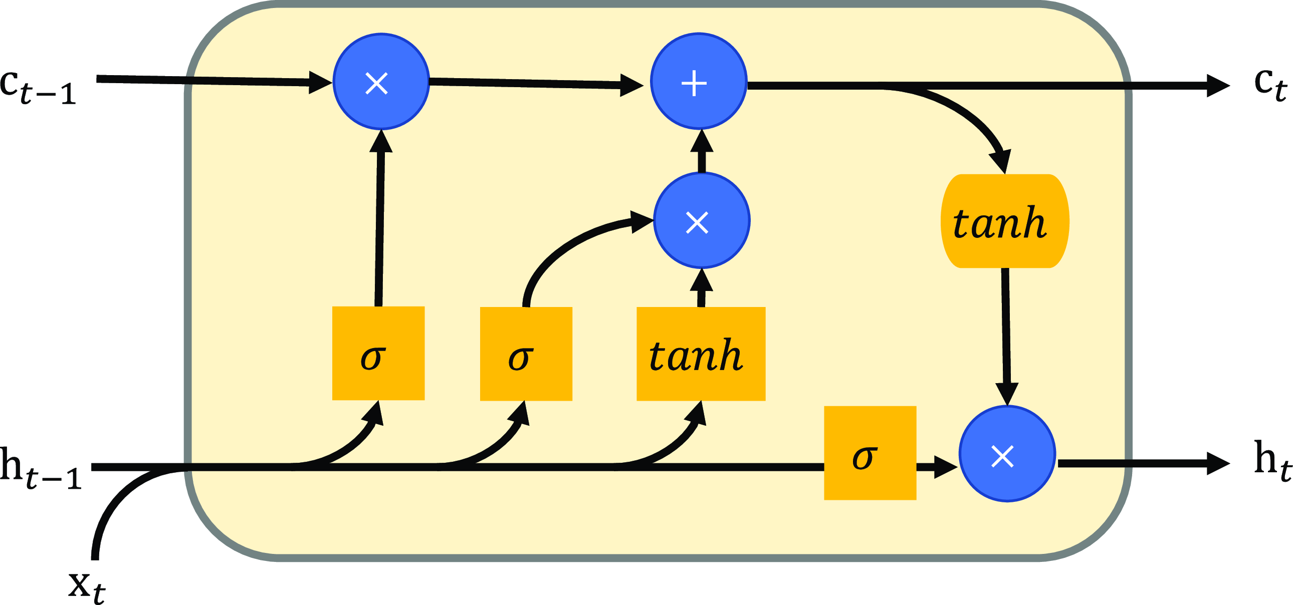
Recurrent Neural Networks (RNNs) are a natural fit for sequential data and thus have been applied to mortality time series. The RNN processes a time series one step at a time, carrying forward a summary of what it has learnt from previous years to the next step. In mortality modeling, this sequential structure can be the Lee-Carter time index. However, RNNs suffer from vanishing gradients in long sequences, where older information gradually fades. Long Short-Term Memory (LSTM) networks resolve this by maintaining an additional cell state, which allows information to be preserved and managed throughout the entire sequence. The cell state uses gate mechanisms to decide what to store, update, and discard (Hochreiter & Schmidhuber, Reference Hochreiter and Schmidhuber1997). Figure 2 shows a unit structure of LSTM. At each time step $t$ , an LSTM cell updates its internal memory and output by using the current input $\mathbf{x}_t$ , the previous hidden state $\mathbf{h}_{t-1}$ , and the previous cell state $\mathbf{c}_{t-1}$ . This architecture preserves both short-term and long-term dependencies whilst still being capable of learning non-linear temporal patterns in mortality data. Figure 3 shows recent studies that have applied RNNs and LSTMs to mortality forecasting.

Figure 2.

Data flow in an LSTM unit at time step $t$ . The input $\mathbf{x}_t$ and previous hidden state $\mathbf{h}_{t-1}$ pass through three gates (forget, input, and output) to compute the new cell state $\mathbf c_t$ and hidden state $\mathbf h_t$ . Yellow boxes denote activations $\sigma$ and $\tanh$ ; and blue circles refer to element-wise multiplication and addition. Adapted from Ingolfsson (Reference Ingolfsson2021).

Figure 3.

Tree of sequence modeling (RNN/LSTM) methods in mortality forecasting.

The Lee–Carter model (Lee & Carter, Reference Lee and Carter1992) models the mortality rates as

(1) \begin{equation} \ln (m_{x,t}) = \alpha _x + \beta _x\,k_t + \varepsilon _{x,t}, \end{equation}

where $\alpha _x$ denotes the average log-mortality at age $x$ , $\beta _x$ is the age-specific sensitivity to the time index $k_t$ , and $\varepsilon _{x,t}$ is the residual error term. The log of mortality $\ln (m_{x,t})$ is first centered by subtracting $\alpha _x$ , and then applying Singular Value Decomposition (SVD) to the resulting age–time matrix. The leading singular vectors give $\beta _x$ and $k_t$ . Finally, $k_t$ is forecasted via a random walk or an ARIMA model, and recombined with $\alpha _x$ and $\beta _x$ to produce mortality forecasts.

The Lee-Carter model assumes a constant Gaussian error variance on the log-mortality rates, yet the error is much larger when death counts are low. To address this, Brouhns et al. (Reference Brouhns, Denuit and Vermunt2002) reframed the model as a Poisson Generalized Linear Model (GLM), namely the Poisson Lee-Carter, for the death counts as

(2) \begin{equation} D_{x,t} \sim \textrm{Poisson}\; \bigl (E_{x,t}\,e^{\alpha _x + \beta _x k_t}\bigr ), \end{equation}

where the exposure $E_{x,t}$ is the the person-years lived at age $x$ in year $t$ . The familiar Lee-Carter parameters $\alpha _x$ , $\beta _x$ , and $k_t$ are now estimated by maximum-likelihood in a Poisson GLM, rather than by SVD. After maximizing the likelihood, the projected period index $k_t$ (from a random walk or ARIMA model) is substituted back to give future death counts.

The ARIMA models used in the Lee-Carter framework may fail to capture non-linear and complex temporal dependencies in mortality trends. Hence, Nigri et al. (Reference Nigri, Levantesi, Marino, Scognamiglio and Perla2019) introduced LSTM to replace the standard ARIMA-based projection of $k_t$ . Mortality rates are reconstructed through the Lee-Carter formula, with LSTM projected $k_t$ achieves superior out-of-sample accuracy across six countries using the Human Mortality Database (HMD) (Human Mortality Database, 2025). Beyond a plain LSTM, Chen & Khaliq (Reference Chen and Khaliq2023) explored alternative variants of RNN architectures, comparing LSTM, Bidirectional LSTM (Bi-LSTM), and Gated Recurrent Unit (GRU) for forecasting $k_t$ on the HMD United States data. They found all three deep learning models achieved comparable performance to Lee–Carter, with the Bi-LSTM performing marginally better due to its bidirectional processing capturing both past and future information.

Although RNN variants can extract rich temporal patterns, reliable calibration of these networks’ parameters becomes difficult when mortality data is scarce in calendar years. Lindholm & Palmborg (Reference Lindholm and Palmborg2022) tackled this problem by combining a traditional Lee-Carter framework with a residual learning LSTM. They first fit a standard Poisson Lee–Carter model to obtain the baseline time index trends, then train the LSTM only on the residuals. The LSTM only had to learn the remaining small non-linear deviations, which is more stable than trying to relearn the whole mortality pattern from limited data. Because short series can give an unrealistic validation result, they proposed three ways of splitting the data. The Last Observation and Random-Time splits take calendar years away from the already short series, so the network sees even fewer observations during training. Sub-Cohort Population instead splits individuals to be training or validation, so the full calendar span is retained to avoid further shortening the series. Applied to HMD populations, the method matches a random walk index performance when trends are linear but outperforms the random walk.

The RNN-based methods we have discussed so far are all on single populations for forecasting in isolation and ignore coherent relationships between populations. Coherent multi-population architectures can be used to link related populations and prevent unrealistic long-term divergence. Traditionally, the Augmented Common Factor (ACF) model (Li & Lee, Reference Li and Lee2005) extended Lee–Carter to multiple populations by combining a set of common factors and population-specific adjustments. Deep neural networks can achieve coherence by sharing information across multiple populations within a single architecture. Bravo (Reference Bravo2021) introduced a simple three-layer LSTM to jointly forecast Portugal mortality for both genders. The LSTM treats calendar year as the time dimension, and at each time step, it injects the age-specific mortality rate with a gender indicator. The network produced smooth, coherent mortality projections across both genders over the entire forecasting horizon and significantly outperformed Lee-Carter for males.

Much of the mortality forecasting literature is focused on point estimations, but actuaries often need calibrated intervals or tail risk understanding for risk assessment. Hence, Marino et al. (Reference Marino, Levantesi and Nigri2023) embedded an LSTM into the Lee-Carter framework and obtained prediction intervals by repeatedly resampling death counts via a Poisson bootstrap. For each sample, they refit the Lee-Carter model and retrain the LSTM on the updated time index, and then use the distribution of these forecasts to form the interval. The method not only yields more accurate point forecasts but also provides more reliable long-term intervals than the traditional method in the three HMD countries separately.

A growing trend in mortality forecasting is to incorporate external covariates, such as environmental, pollution, and fine-grained regional data into mortality forecasting (Dimai, Reference Dimai2024). This means actuaries can understand the explicit risk drivers for mortality prediction, which enables them to support scenario testing for pricing and reserving decisions. Robben et al. (Reference Robben, Antonio and Kleinow2024) introduced a two-stage machine learning framework, first isolating seasonal trends with a Serfling model, followed by a machine learning model (XGBoost) on weather and pollution anomalies (European Centre for Medium-Range Weather Forecasts (ECMWF), 2023; Eurostat, 2024) to capture residual spikes. Building on this, Zheng et al. (Reference Zheng, Wang, Zhu and Xue2025) introduced MortFCNet, a simple deep architecture combining GRU and fully connected networks to predict multi-population weekly death rates based on region-specific weather inputs. The GRU, a lighter RNN variant, is used to capture temporal dependencies in weekly mortality and weather sequences. It also has a downstream fully connected (feed-forward) MLP head, which transforms the GRU’s final hidden state into region-specific death-rate predictions. Unlike Serfling-based methods and gradient boosting models, which depend on predefined Fourier terms and manual feature engineering, MortFCNet learns patterns directly from raw time-series data, hence showing superior prediction performance to existing methods over 200 fine-grained regions.

In summary, RNNs became effective for mortality forecasting once the domain knowledge (e.g., the Lee–Carter structure) was integrated, the data limitations were tackled with sophisticated training methods (e.g., ensembles or boosting), multi-population extensions enforced the coherence, the interpretability was enhanced with interval estimations, and external covariates were used to help capture short-term mortality volatilities. While RNNs excel at learning temporal dynamics, plain (ungated) RNNs can struggle with very long forecasting horizons due to vanishing gradient; separately, cohort effects across age groups are not captured by default and require explicit cross-age links (e.g., shared latent factors or cohort covariates).

2.2. Attention mechanisms: transformers

Transformers followed RNNs into mortality forecasting to address the vanishing gradient limitation, because the self-attention mechanism in Transformers allows every time point to weigh all others and capture long-term dynamics (Vaswani et al., Reference Vaswani, Shazeer, Parmar, Uszkoreit, Jones, Gomez, Kaiser and Polosukhin2017).

Figure 4 shows the flow of information in a 1-D self-attention module. The input time series (e.g, the Lee-Carter time index $k_t$ ) is linearly projected via the weight matrices $W_Q$ , $W_K$ , and $W_V$ to obtain the matrices of queries $Q$ , keys $K$ , and values $V$ . The matrix multiplication $QK^{\top }$ measures the similarity between every pair of time points. Applying a softmax to each row converts these scores into attention weights that sum to one for each query time step. Each time step is then updated by a weighted sum of the $V$ vectors across all times, so highly similar parts of the sequence exert greater influence. The resulting vectors then pass through an output-projection layer $W_o$ to realign dimensionality. This adaptive mechanism highlights the most relevant information before the resulting representation is passed to the next stage of the Transformer (Zhang et al., Reference Zhang, Goodfellow, Metaxas and Odena2019). Recent studies of Transformers for mortality forecasting are shown in Figure 5.

Figure 4.

Diagram of a 1-D self-attention module for projecting the mortality time index $k_t$ . The input sequence is projected by $W_Q$ , $W_K$ , and $W_V$ to queries $Q$ , keys $K$ , and values $V$ . Soft-maxed similarity scores $QK^{\top }$ provide attention weights that re-scale $V$ , then the weighted result passes through an output-projection layer (via $W_o$ ) to produce an output that highlights the most relevant information. Adopted from Zhang et al. (Reference Zhang, Goodfellow, Metaxas and Odena2019).

Figure 5.

Tree of attention-based (Transformers) methods in mortality forecasting.

Roshani et al. (Reference Roshani, Izadi and Khaledi2022) were among the first to incorporate a Transformer self-attention network within a two-step Poisson–Lee–Carter framework, using it to forecast the Lee–Carter time index $k_t$ . They applied this approach to 11 HMD populations. The Transformer showed clear improvement over the LSTM and ARIMA baselines, particularly for longer forecasting horizons. However, the two-stage process propagates estimation error from the Lee–Carter fit into the Transformer stage.

To close this gap, Wang et al. (Reference Wang, Wen, Xiao and Wang2024) replaced the two-step process with a single-stage Transformer that forecast mortality rates for each of the eight HMD countries. An embedding layer first extracts the spatial age structure, while positional encoding is used to preserve the calendar order of the sequence. The multi-head self-attention block then allows each age-specific mortality rate to attend to every other across time, capturing long-range temporal dependencies that RNNs may miss, and a feed-forward network to predict mortality rate. Empirical tests showed that the Transformer outperformed the traditional Lee-Carter model and deep baselines (RNN, LSTM, and CNN) in predictive accuracy across all countries, particularly for older populations. However, because a separate model is fitted for each country, parameters are not shared across populations, leaving cross-country information unexploited.

Hence, Shen et al. (Reference Shen, Yang, Liu and Li2024) extended Transformers to share information explicitly across countries by introducing GT-A. The GT-A combines Graph Convolutional Networks (GCNs) to create cross-country links, with Transformers to forecast mortality rates for European HMD countries. First, Principal Component Analysis (PCA) is used to reduce the age dimension, then a $K$ -means is used to cluster countries according to Dynamic Time Warping (DTW) similarities. These clusters form the graph nodes, with edges capturing spatial and demographic relationships, forming an adaptive adjacency matrix. The matrix supplies the weights that GCN use when propagating information between nodes, capturing spatial links among clusters, while the Transformer models the temporal patterns within each node. In such a way, GT-A produces lower forecast errors than both the Lee-Carter and other neural baselines on 16 HMD populations.

In summary, Transformers entered mortality modeling because their self-attention inspects the entire age–period surface at once. It detects long-term links that recurrent and traditional time-series models often miss. Despite the benefits, transformer models only deliver point estimations without uncertainty quantification.

2.3. Latent-variable modeling: autoencoders

In mortality forecasting, AEs have also received attention, as methods such as Variational Autoencoder (VAE) can provide direct probabilistic forecasts that Transformers and other deep methods struggle to provide for actuaries to better assess risks. AEs are unsupervised neural networks designed to decompose high-dimensional inputs into latent representations and then reconstruct the original data from them. An AE, therefore, has two blocks, an encoder to non-linearly embed the input data into a low-dimensional latent space and a decoder to reconstruct the original data from this compressed representation. In mortality research, plain AEs can be used to reduce the age-period mortality source into a set of interpretable latent factors, but they return a point forecast. The VAE advances this idea by treating the latent representation as a probability distribution instead of a single deterministic vector. During training, the VAE learns both a mean and a variance for each latent dimension, allowing it to generate multiple plausible outcomes rather than a single point estimate (Kingma & Welling, Reference Kingma and Welling2014).

Figure 6 illustrates how a VAE probabilistically reconstructs mortality data. The age-specific average $\alpha _x$ from Lee-Carter is first subtracted from the log-mortality rate $\log (m_{x,t})$ to form the input vector $\mathbf{X}(t)$ . The encoder maps $\mathbf{X}(t)$ to a Gaussian distribution of mean $\boldsymbol \mu$ and standard deviation $\mathbf{s}$ , and a latent vector $\mathbf{z} = \boldsymbol \mu + \mathbf{s}\odot \boldsymbol \epsilon$ is sampled. The decoder reconstructs $\hat {\mathbf{X}}(t)$ from $\mathbf{z}$ , which then adds back $\alpha _x$ to recover the reconstructed log-mortality rates. Because the latent vector $\mathbf{z}$ is sampled from the latent probabilistic space, the decoder’s output $\hat {\mathbf{X}}(t)$ is a random variable; repeated sampling of $\mathbf{z}$ generates a PD rather than a single point forecast. Recent studies of AE for mortality forecasting as shown in Figure 7.

Figure 6.

VAE probabilistic reconstruction. The encoder transforms $\mathbf{X(t)}$ into a latent probabilistic space with mean $\boldsymbol \mu$ and scale $\mathbf{s}$ , from which $\mathbf{z}$ is sampled by using noise $\boldsymbol \epsilon$ . The decoder then reconstructs $\hat {\mathbf{X}}(t)$ from $\mathbf{z}$ (Miyata & Matsuyama, Reference Miyata and Matsuyama2022).

Figure 7.

Tree of latent-variable modeling (Variational autoencoders) methods in mortality forecasting.

The deterministic point-forecast plain neural network autoencoder (AE) was first applied to mortality forecasting by Hainaut (Reference Hainaut2018). This encoder compresses mortality data into low-dimensional latent factors, which are then projected forward via a simple random walk; the decoder subsequently reconstructs the full age-specific mortality rate. Importantly, the decoder $f_{\text{dec}}$ transforms the one-dimensional latent index $\kappa _t$ into an age-profile $f_{\text{dec}}(x,\kappa _t)$ , which mirrors Lee–Carter’s $\beta _x k_t$ , so the resulting curve over age is a familiar and interpretable sensitivity pattern. Results from France, the UK, and the US show that the AE significantly outperformed Lee-Carter, confirming that latent factors better summarize mortality trends whilst maintaining the interpretability.

Continuing the theme of interpretability, Tanaka & Matsuyama (Reference Tanaka and Matsuyama2025) developed an interpretable neural network for cause-of-death mortality forecasting. The model is a one-dimensional convolutional autoencoder (CAE) that replaces the traditional Lee–Carter tensor factorization. The encoder compresses high-dimensional cause-of-death data (World Health Organization, 2025) into a low-dimensional latent representation. By constraining the latent layer to one dimension, the CAE learns Lee-Carter-like time index $\kappa _t$ , then the decoder converts it into a cause ( $c$ ) and age-specific sensitivity curve similar to the $\beta _{x,c}$ , where the mapping from $\kappa _t$ to $f_{\textrm{dec}}(x,c,\kappa _t)$ remains directly interpretable. Here, $f_{\textrm{dec}}(x,c,\kappa _t)$ denotes the decoder that maps age $x$ , cause $c$ , and the time index $\kappa _t$ to the reconstructed log-mortality. The CNN enables parameter sharing and modeling the relationship between different causes of death. Tested in Japan, the United Kingdom, and Germany, Tanaka & Matsuyama (Reference Tanaka and Matsuyama2025) show that the CAE outperforms tensor factorization benchmarks while maintaining interpretability. However, AE models provide only point estimations.

AEs are useful for interpretable point estimations, but VAEs provide built-in probabilistic latent representations that plain AEs and Transformers lack. Miyata & Matsuyama (Reference Miyata and Matsuyama2022) embedded a VAE inside the Bayesian state-space (BSS) framework, with uncertainties handled by the BSS and the non-linear using a neural network decoder. Specifically, they formulated the log-mortality by keeping a latent factor $z_t$ that evolves as a drifted random walk (similar to the Lee-Carter time index $\kappa _t$ ), and the Lee-Carter structure $\alpha _x + \beta _x \kappa _t$ is replaced with a neural network decoder $f_{\theta }(z_t)$ which maps the latent factor to age-specific mortality rates. Because the BSS backbone already provides endogenous randomness, the model outputs internally calibrated confidence intervals, and the VAE estimator delivers without the heavy Markov Chain Monte Carlo (MCMC) sampling, such as random seeds, required by other neural networks. Empirical tests on HMD data show that the VAE achieves forecast errors at least as low as, and in several cases lower than, the standard Lee–Carter benchmark while providing the interval coverage.

In summary, applying AEs in mortality forecasting combines deep learning, probabilistic uncertainty modeling, and interpretable latent representations. This approach manages the black-boxes criticism by providing an interval estimation and by revealing interpretable latent factors to enhance the interpretability, but the current architecture designs do not capture cohort effects, as the latent time process is simplified to keep the estimation manageable.

2.4. Spatial grid modeling: Convolutional Neural Networks (CNNs)

CNNs followed RNNs to capture cohort effects between age groups, which was also a limitation of the AEs. CNNs use learnable filters that move across small neighborhoods of a matrix, enabling them to recognize local spatial and temporal patterns. In mortality forecasting, the input can be mortality rates arranged as a two-dimensional matrix, with rows representing years and columns representing age groups. Unlike RNNs, which process one year at a time, CNN filters slide across adjacent ages and years to capture the diagonal cohort effects. As these convolutions are shift-invariant, patterns such as sudden mortality spikes learnt in one part of the grid transfer to other ages and cohorts, which allows better generalizations (Zhang et al. Reference Zhang, Chen and Liu2022).

Figure 8 illustrates that, in a CNN, the input passes through several layers in sequence and each layer transforms the input in specific ways to help the network learn useful patterns. The input here is a mortality matrix for a country, where rows represent years and columns represent age groups. Each convolutional layer applies learnable filters, performing a weighted sum and outputs a new value into the feature map. The max pooling layer then downsamples the feature maps by keeping the most prominent value (maximum) to reduce dimensionality. The resulting features are then passed to dense layers to predict the mortality rate (LeCun et al., Reference LeCun, Bottou, Bengio and Haffner1998). Recent applications of CNN methods in mortality forecasting are shown in Figure 9.

Figure 8.

Data flow in a CNN block. The input is a 2D mortality matrix. The matrix is processed by sliding over a set of filters that the network learns during training, passing through an activation, and then being downsampled by max pooling. The resulting features are flattened and fed into a dense layer to produce the final mortality rate output (GeeksforGeeks, 2025; Podareanu et al., Reference Podareanu, Codreanu, Aigner, Leeuwen and Weinberg2019).

Figure 9.

Tree of spatial grid modeling (CNN) methods in mortality forecasting.

Both Perla et al. (Reference Perla, Richman, Scognamiglio and Wüthrich2021) and Wang et al. (Reference Wang, Zhang and Zhu2021) employed CNNs for age–period multi-population mortality forecasting. Perla et al. (Reference Perla, Richman, Scognamiglio and Wüthrich2021) implemented a one-dimensional (1D) CNN along each age’s time series, capturing temporal patterns in mortality improvements. Their results show that even a simple CNN outperforms traditional stochastic models on HMD and the US Mortality Database (UMD) (University of California, Berkeley 2025). However, processing each age separately prevents the 1D CNN from learning interactions across age or cohorts across the full mortality grid. By contrast, Wang et al. (Reference Wang, Zhang and Zhu2021) framed mortality data as a two-dimensional (2D) matrix (ages by years). This allows the CNN to scan both age and time, detecting local patterns such as cohort effects. Their two-dimensional model captures dependency structures that a 1D approach might miss by incorporating these neighborhood interactions. Out-of-sample tests on 41 HMD populations confirm superior performance to traditional models. Notably, Wang et al. (Reference Wang, Zhang and Zhu2021) also showed that the framework can be extended to multi-population data.

Since CNNs capture local spatial dependencies but struggle to capture the long-range temporal dynamics important for mortality improvements, later studies have paired them with sequence models, such as LSTM networks. Zhang et al. (Reference Zhang, Chen and Liu2022) therefore proposed a hybrid LSTM–CNN model for multi-population mortality forecasting, enabling the network to learn shared information across 21 HMD populations. In this architecture, the LSTM captures long-term temporal dependencies (mortality improvement trends), while the CNN extracts local age–period features via 2D convolutions. By merging these components, the model embeds an age–period–cohort structure within the network. On HMD data, the model produced the most accurate long-term forecasts, outperforming stand-alone CNNs, stand-alone LSTMs, and traditional benchmarks.

Overall, CNNs excel at detecting local age-period patterns, and when compared with LSTMs, they further improve long-range accuracy. However, the shared kernels of CNNs impose shift invariance, assuming that the same pattern reappears everywhere on the mortality surface. This can blur location-specific cohort variations.

2.5. Locally connected & multi-task neural networks

LCNs can retain convolutional strengths while capturing position-specific mortality patterns that the standard CNNs miss. FNNs are neural networks in which information flows in a single direction without any cycles or loops. The CNN described above is an FNN, and an LCN is a CNN variant without weight sharing. As illustrated in Figure 10, the fully connected feed-forward network (FFN) links every unit in one layer to every unit in the next, and ignores any spatial information. The CNNs discussed earlier process inputs by having each neuron in a convolutional layer look only at a small patch of the input to capture local patterns, and then share the same learnable filter across all positions. In contrast, LCNs preserve local connectivity, where each unit only connects to a restricted set of units and uses distinct filters for each region. Figure 11 illustrates recent studies of LCNs and other FNNs in mortality forecasting.

Figure 10.

Comparison of a locally connected layer versus a fully connected and a convolutional layer. In (a) the fully connected structure, each of the three output units is connected to all input units; in (b) the locally connected structure, each output unit has its own set of weights; and in (c) the convolutional structure, there is a single shared filter applied across all positions. The figures are adapted from Scognamiglio (Reference Scognamiglio2022).

Figure 11.

Tree of locally connected and multi-task network methods in mortality forecasting.

Scognamiglio (Reference Scognamiglio2022) tackled the multi-population shortcomings of the Lee-Carter model by using neural networks. Their architectures mirror the Lee-Carter setup by simultaneously learning the parameters (age intercept, sensitivity, and time index) for each population. They explored three networks, Fully Connected Layer (FCL), LCN, and CNN, and found LCN to be the most effective for its local connectivity. The pooling across multiple HMD populations produced smoother parameters and achieved better accuracy than the traditional Lee-Carter calibration. This shows LCNs can improve forecasts while retaining the model’s age-period interpretability.

Pursuing the same balance of accuracy and interpretability, Richman & Wüthrich (Reference Richman and Wüthrich2023) proposed LocalGLMNet, an FNN with a skip connection that preserves the additive form of a Generalized Linear Model (GLM) while allowing weights to be learnt non-linearly. The skip connection sends each input straight to the final output layer, so the prediction is an intercept plus the sum of feature-wise products between inputs and a learnt weight. If the weights remain constant across inputs, the model reduces to the ordinary GLM.

LocalGLMNet was introduced for tabular insurance data. Building on that foundation, Perla et al. (Reference Perla, Richman, Scognamiglio and Wüthrich2024) extended the LocalGLMNet (Richman & Wüthrich, Reference Richman and Wüthrich2023) and applied it to mortality grids; they (i) replaced the FCL with LCN so GLM coefficients can vary by age and time for each population smoothly, and capture localized patterns, (ii) used a denoising AE to filter measurement noise in the data, and (iii) added regularization to further enhance the forecast accuracy. On the HMD populations, the regularized LocalGLMNet surpassed both locally connected convolution benchmarks and the Lee–Carter model. Moreover, they applied a fine-tuned transfer-learned LocalGLMNet variant, which demonstrated superior accuracy when the model was trained on HMD and applied to the UDM datasets. Although the refined LocalGLMNet delivered more accurate point forecasts, it offers no information about forecast uncertainties that actuaries need.

Responding to the gap above, Corsaro et al. (Reference Corsaro, Marino and Scognamiglio2024) recognized that insurers need the full distribution of mortality outcomes beyond just the mean mortality rate. Hence, they introduced a jointly calibrated neural network quantile Lee–Carter model that learns all populations simultaneously. They fitted a shared embedding-based network to produce each population’s age intercept $a_x$ and sensitivities $\beta _x$ instead of separate SVD or quantile regressions for each population. A two-layer feed-forward network (LCN followed by FCN) trained the time index $k_t$ . The network is trained separately for each quantile (0.05, 0.10, 0.50, 0.90, 0.95). Results on HMD populations show that the jointly calibrated model outperformed both the traditional Lee-Carter average model and the single-population quantile models fitted separately. Additionally, multi-population extreme-quantile forecasts are more reliable than single-population models fitted separately. However, although Corsaro et al. (Reference Corsaro, Marino and Scognamiglio2024) took a step towards distributional information by providing quantile curves, each predicted quantile remains a point prediction, and the method does not quantify the model or parameter uncertainty.

Extending Lee-Carter models to handle diverging population trends, Perla & Scognamiglio (Reference Perla and Scognamiglio2023) proposed the Locally Coherent Multi-Population Neural Network, which combines a learnable country embedding with a relaxed coherence assumption. In this model, each country is represented by a learnt low-dimensional vector (the country embedding); hence, countries with similar age-period patterns cluster naturally in the latent space. The relaxed coherence refers to allowing separate clusters to share their own trends. Within each cluster, FCN layer is used to refine the age intercept and sensitivities, preserving the Lee-Carter interpretability whilst capturing local non-linearities. The model yields lower out-of-sample MSE than single-population Lee–Carter models and the fully-coherent ACF benchmark.

The above studies are concentrated on retaining an explicit Lee-Carter or GLM structure and estimating their covariates. Studies have also applied FNNs to learn directly from the mortality surface. Richman & Wüthrich (Reference Richman and Wüthrich2021) proposed a single-task FNN for multi-population forecasting. The approach was to train an FNN across all populations simultaneously, with combined data from various ages, years, genders, and countries, to predict the mortality rate for a single combination of inputs. The hidden layers are shared by all countries, and a country-embedding layer is used to distinguish different countries. This allows the model to learn shared mortality patterns across populations. While the model outperformed Lee-Carter and its variants for populations with similar trends, the accuracy deteriorated when mortality patterns diverged.

To address the performance drop of using single-task networks when mortality patterns diverge, De Mori et al. (Reference De Mori, Haberman, Millossovich and Zhu2025) proposed a hierarchical multi-task design to have a controlled way for pooling countries that have similar mortality trends. They first explicitly clustered 17 HMD populations with $K$ -means to group countries with similar life expectancy changes. Embedded inputs (year, age, sex, and country) are passed through three fully connected dense layers that learn representations common to every country. Subsequently, a cluster-specific dense layer is added to capture the pattern within clusters. This design draws strength from countries with larger datasets and achieves lower out-of-sample errors than both single-task networks and Lee-Carter benchmarks.

In summary, LCNs bridge FFNs and CNNs, capturing location-specific mortality patterns while limiting the number of parameters. When embedded in the Lee-Carter framework or an interpretable LocalGLMNet, LCN consistently demonstrated superior accuracy. Multi-task feed-forward network models share information across populations to reduce overfitting and improve accuracy.

3.1. Remaining challenges

Current deep learning models for mortality forecasting still face several important limitations. First, uncertainty quantification remains weak, as most recurrent, convolutional, Transformer, LCNs, and Multi-Task FNNs yield only point forecasts, offering no built-in measures of predictive uncertainty. Plain VAEs improve this, where the encoder outputs the Gaussian mean and variance. The Bayesian VAEs by Miyata & Matsuyama (Reference Miyata and Matsuyama2022) produced a probabilistic latent representation by capturing the parameter uncertainty. To manage model complexity, they modeled the latent factors as a one-dimensional random walk, with independent residuals and a single-neuron final layer. However, the simple structure cannot capture cohort effects or be used for multi-population forecasting.

Second, interpretability is important for actuarial decision-making; however, interpretability is limited and varies across architectures. For example, the filters of a CNN excel at capturing localized patterns, but these features do not readily translate into global age-period-cohort narratives familiar to actuaries. Furthermore, architectures like Transformers (Shen et al., Reference Shen, Yang, Liu and Li2024) remain largely opaque, failing to provide time index and age-period sensitivities analogous to Lee-Carter.

Third, multi-population mortality forecasting is still imperfect. For example, recent multi-task and graph-based models in mortality modeling (De Mori et al., Reference De Mori, Haberman, Millossovich and Zhu2025; Shen et al., Reference Shen, Yang, Liu and Li2024) rely on heuristic $K$ -means clustering to assign countries to groups. Although $K$ -means aims to minimize within-cluster variation (MacQueen, Reference MacQueen1967), and thus echoes the idea of Li & Lee (Reference Li and Lee2005) that reducing heterogeneity can improve multi-population forecasting, the method is unsupervised and not linked to forecasting loss. As a result, the clustering outcome may not reflect demographic similarity and may not guarantee predictive accuracy improvement. Moreover, the relationship between countries in multi-population mortality forecasting often ignores temporal changes in mortality trends over time. For example, Shen et al. (Reference Shen, Yang, Liu and Li2024) modeled country relationships by GCN, and Robben et al. (Reference Robben, Antonio and Kleinow2024) adopted an adjacent matrix in the penalty to incorporate smoothness across neighboring regions; although the methods explored spatial relationships, these relationships are assumed to be static.

Fourth, data scarcity at extreme ages or in small regions continues to undermine model stability, even when information is pooled across populations. For example, Richman & Wüthrich (Reference Richman and Wüthrich2023) noted that model weights become unpredictable for older age groups, and accuracy is lower for smaller populations.

Fifth, some areas in mortality forecasting are under-explored with deep learning, for example, deep learning models for cause-of-death mortality forecasting (Tanaka & Matsuyama, Reference Tanaka and Matsuyama2025). In addition, many recent and advanced deep learning methods and architectures, such as diffusion models (Ho et al., Reference Ho, Jain and Abbeel2020) and Mamba (Gu & Dao, Reference Gu and Dao2023), are still unexplored in mortality forecasting.

Finally, marginal gains in predictive accuracy offer limited actuarial value if they come at the expense of interpretability or make uncertainty quantification impractical. Actuarial work relies not only on point forecasts, but also on well-calibrated, explainable measures of uncertainty, particularly under regulatory frameworks.

3.2. Future directions

These shortcomings point to several directions for future work. First, to address the weak uncertainty quantification, Monte Carlo sampling from the latent space could be used to generate the confidence interval from the plain VAE, as similarly suggested for future work by Apellániz et al. (Reference Apellániz, Parras and Zazo2024) in the survival analysis. Moreover, hierarchical Bayesian methods could be combined with deep learning for multi-population mortality forecasting with uncertainty quantification.

Second, to tackle the limited interpretability, tailored interpretability tools, such as SHapley Additive exPlanations (SHAP) values (Lundberg & Lee, Reference Lundberg and Lee2017), could be adapted to mortality grids to map deep network components back to interpretable actuarial age, period, and cohort factors, making the motivation behind forecasting easier to explain.

Third, for multi-population mortality forecasting, instead of the heuristic grouping, a clustering layer can be constructed to cluster the populations under the supervision of the prediction loss. Moreover, to cover both the relationship between countries/regions and the dynamic temporal changes of mortality data (e.g., to induce a temporal index into the spatial adjacency matrix), spatio-temporal deep models can be explored.

Fourth, to overcome the data scarcity when forecasting the mortality rates, it can be helpful to integrate external covariates such as vaccination coverage, socioeconomic indicators, or environmental factors (Wang et al., Reference Wang, Wen, Xiao and Wang2024).

Fifth, it merits further exploration of deep learning models for cause-of-death mortality forecasting, for example, by using multi-task deep learning models and graph neural networks to model the relationship between causes. It is also worthwhile to explore the latest deep learning methods and architectures, such as Mamba and diffusion models, for mortality forecasting, because they have shown promising performance in modeling time series and spatio-temporal data in other areas like computer vision and pattern recognition. For example, Mamba-type selective state-space models offer efficient long-context sequence modeling (linear time); when paired with cohort information, they could better capture slow cohort trends and help stabilize forecasts for data-sparse ages, small regions, and rare causes. Conditional/score-based diffusion models yield samples from an approximate PD, enabling principled uncertainty quantification (via Monte Carlo quantiles).

Finally, although these future directions mitigate specific shortcomings, they do not yet resolve the overarching challenges of actuarial modeling. The development of actuarial models should balance predictive performance, complexity, uncertainty, and interpretability.