


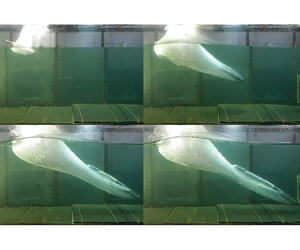



1. Introduction
Water entry of vehicles widely exists in the fields of aeronautics, astronautics and military weapons, i.e. aerial-underwater and air-drop vehicles. With the development of technology, the water-entry velocity of vehicles is increasing, reaching hundreds of metres per second. The process of high-speed water entry is a transient process with strong nonlinear characteristics. In this process, the vehicle structure suffers severe hydrodynamic loads which may not only cause the deformation and damage of the thin structures but also lead to the malfunction of internal instruments. Moreover, the hydrodynamic loads affect and determine the characteristics and stability of the trajectory. High-speed water entry usually occurs within a very short period of time and is usually accompanied by nonlinear flow phenomena such as water impact, free surface splash, air entrainment and cavity evolution. Such behaviour poses great challenges in fluid mechanics.
High-speed water entry is a classical hydrodynamic problem. The related water-entry work can be found dating back to the beginning of the last century. The pioneering work on the theoretical research of water impact was carried out by Von Kármán (Reference Von Kármán1929) and Wagner (Reference Wagner1932). Then, for impacting bodies with small deadrise angles, Cointe & Armand (Reference Cointe and Armand1987) and Howison, Ockendon & Wilson (Reference Howison, Ockendon and Wilson1991) further developed and extended Wanger's theory through the matched asymptotic expansions. Dobrovol'skaya (Reference Dobrovol'skaya1969), Semenov & Iafrati (Reference Semenov and Iafrati2006) and Semenov & Wu (Reference Semenov and Wu2016) presented similarity solutions for wedges that enter the water surface with a constant velocity. Previous methods were designed and developed for two-dimensional asymmetric objects (Semenov & Iafrati Reference Semenov and Iafrati2006; Faltinsen & Semenov Reference Faltinsen and Semenov2008; Semenov & Wu Reference Semenov and Wu2019), arbitrary section bodies (Zhao & Faltinsen Reference Zhao and Faltinsen1993; Mei, Liu & Yue Reference Mei, Liu and Yue1999), axisymmetric three-dimensional objects (Shiffman & Spencer Reference Shiffman and Spencer1951; Hulin et al. Reference Hulin, Del Buono, Tassin, Bernardini and Iafrati2022) and three-dimensional simple objects (Korobkin & Scolan Reference Korobkin and Scolan2006; Tsaousis, Papadopoulos & Chatjigeorgiou Reference Tsaousis, Papadopoulos and Chatjigeorgiou2020). However, these studies are based on potential flow theory, and the liquid is assumed to be incompressible. When the impact velocity is high and/or the object is blunt enough, it is necessary to take into account the compressibility of the fluid (Skalak & Feit Reference Skalak and Feit1966; Korobkin & Pukhnachov Reference Korobkin and Pukhnachov1988). Previous researchers examined the impact of water on compressible fluids (Korobkin Reference Korobkin1992, Reference Korobkin1994). However, in most cases, the liquid is assumed to be ideal and weakly compressible, and shock waves induced by the impact are described based on the acoustic approximation. Eroshin's experiments indicated that the maximum impact force by the linear acoustic approximation is lower than the experimental results for high-speed water entry (Eroshin et al. Reference Eroshin, Romanenkov, Serebryakov and Yakimov1980). Furthermore, the theoretical methods have two other limitations: they are only suitable for the initial stage of water-entry processes, and the presence of air is not taken into account.
In addition to theoretical research, researchers have also carried out various water-entry experiments including different nose shapes (Thoroddsen et al. Reference Thoroddsen, Etoh, Takehara and Takano2004; Truscott, Epps & Techet Reference Truscott, Epps and Techet2012; Bodily Reference Bodily2013; Marston et al. Reference Marston, Truscott, Speirs, Mansoor and Thoroddsen2016), spinning bodies (Truscott & Techet Reference Truscott and Techet2009; Kiara, Paredes & Yue Reference Kiara, Paredes and Yue2017), hydrophobic and hydrophilic objects (Aristoff & Bush Reference Aristoff and Bush2009; Techet & Truscott Reference Techet and Truscott2011; Yi et al. Reference Yi, Li, Jiang, Lohse, Sun and Mathai2021) and air cushion effects (Chuang Reference Chuang1966; Eroshin et al. Reference Eroshin, Plyusnin, Romanenkov, Sozonenko and Yakimov1984; Ermanyuk & Ohkusu Reference Ermanyuk and Ohkusu2005; Ma et al. Reference Ma, Causon, Qian, Mingham, Mai, Greaves and Raby2016). Published research on high-speed water entry is rare. Several experimental studies looked at the trajectory and cavity of high-speed projectiles (Abelson Reference Abelson1970; Waugh & Stubstad Reference Waugh and Stubstad1972; Hrubes Reference Hrubes2001; Shi & Kume Reference Shi and Kume2001; Truscott Reference Truscott2009; Chen et al. Reference Chen, Huang, Zhang, Qi and Guo2019b; Kiyama et al. Reference Kiyama, Mansoor, Speirs, Tagawa and Truscott2019; Guo et al. Reference Guo, Chen, Mu and Zhang2020), and the research on strong loading is insufficient (May & Woodhull Reference May and Woodhull1948; Eroshin et al. Reference Eroshin, Romanenkov, Serebryakov and Yakimov1980; Truscott, Epps & Belden Reference Truscott, Epps and Belden2014). Due to the limitations of experimental technology and measurement equipment, the size of the experimental projectile is relatively small, and the collection of experimental information and data is difficult.
With the advancement of computer technology, computational fluid dynamics (CFD) techniques have gradually become an important and useful tool to solve high-speed water-entry problems and have the advantage of capturing the detailed characteristics of flow fields. Zhao & Faltinsen (Reference Zhao and Faltinsen1993), Iafrati (Reference Iafrati2000) and Wu, Sun & He (Reference Wu, Sun and He2004) developed the boundary element method (BEM) with a jet flow approximation for the two-dimensional water entry with arbitrary cross-section. Battistin & Iafrati (Reference Battistin and Iafrati2003), Sun & Wu (Reference Sun and Wu2013) and Wu & Sun (Reference Wu and Sun2014) extended the BEM to an axisymmetric model and a three-dimensional model. Park, Jung & Park (Reference Park, Jung and Park2003) developed the source plane method to compute the impact forces and ricochet behaviour of the body during water entry. In addition, various approaches were proposed and developed to study water-entry problems, including smoothed particle hydrodynamics (SPH) method (Oger et al. Reference Oger, Doring, Alessandrini and Ferrant2006; Yuan et al. Reference Yuan, Hong, Zhao and Gong2022) and finite volume method (FVM) (Kleefsman et al. Reference Kleefsman, Fekken, Veldman, Iwanowski and Buchner2005; Hong, Wang & Liu Reference Hong, Wang and Liu2019). In terms of high-speed water entry, preliminary research has been carried out, mainly focusing on impact load (Hong et al. Reference Hong, Wang and Liu2019), load-reducing buffers (including various foam materials, springs and so on) (Shi, Gao & Pan Reference Shi, Gao and Pan2019; Li et al. Reference Li, Sun, Zong, Li and Zhao2021a; Li, Zong & Sun Reference Li, Zong and Sun2021b), trajectory and stability (Li, Lu & Cai Reference Li, Lu and Cai2020; Wang et al. Reference Wang, Shi, Pan, Chen and Zhao2021), cavity formation and evolution (Guo et al. Reference Guo, Zhang, Xiao, Wei and Ren2012; Chen et al. Reference Chen, Sun, Wei and Wang2019a; Sun et al. Reference Sun, Zhou, Yin and Zong2020), etc. To date, numerical research on high-speed water impact is not rich, and the tail slamming phenomenon has rarely been addressed. The strong impact and strong nonlinearity of high-speed water entry pose great challenges to the robustness and stability of CFD methods.
Among the various CFD methods, the immersed boundary (IB) method (Iaccarino & Verzicco Reference Iaccarino and Verzicco2003; Mittal & Iaccarino Reference Mittal and Iaccarino2005; Griffith & Patankar Reference Griffith and Patankar2020) is an important approach for fluid–structure interaction (FSI) problems and is widely utilized due to its excellent ability to deal with complex boundaries (Mittal et al. Reference Mittal, Dong, Bozkurttas, Najjar, Vargas and von Loebbecke2008; Luo et al. Reference Luo, Wang, Tan and Fan2019; Zhou et al. Reference Zhou, Li, Wang, Mu and Zhao2020; Ou et al. Reference Ou, Chi, Guo and Thévenin2022). The IB method employs Euler grids for the flow field and Lagrangian grids for the boundary to address the FSI problems (see figure 1) and introduces body forces into the momentum equation to represent the effect of complex boundaries on the flow. The key challenge in developing the IB methods is the calculation of the body force. Calculation of the body force for the rigid boundary includes the penalty IB method (Goldstein, Handler & Sirovich Reference Goldstein, Handler and Sirovich1993; Lai & Peskin Reference Lai and Peskin2000; Kim Reference Kim2003; Kim & Peskin Reference Kim and Peskin2016) (also known as the feedback forcing method) and the direct forcing method (Mohd-Yusof Reference Mohd-Yusof1997; Fadlun et al. Reference Fadlun, Verzicco, Orlandi and Mohd-Yusof2000). In the first method, a rigid boundary is attached to an equilibrium location by a damped oscillator with a zero resting length. The empirical coefficients (i.e. spring constant and damped coefficient) are employed in the calculation of the body force, which may cause severe stability constraints or spurious elastic effects. In the second method, the direct forcing method proposed by Mohd-Yusof (Reference Mohd-Yusof1997) removes the uncertainties of the empirical coefficients, and velocity reconstruction is employed to calculate the force. However, severe force oscillations usually occur for flows with moving boundaries. Yang et al. (Reference Yang, Zhang, Li and He2009) and Gazzola et al. (Reference Gazzola, Chatelain, van Rees and Koumoutsakos2011) recommended that the smooth discrete delta function be employed to avoid the spurious elastic effects and force oscillations mentioned above. The implicit scheme is also recommended since the boundary condition can be satisfied easily (Le et al. Reference Le, White, Peraire, Lim and Khoo2009; Obeidat & Bordas Reference Obeidat and Bordas2019; Yu & Pantano Reference Yu and Pantano2022). Different IB methods have their own advantages and disadvantages for flows with moving boundaries. Such deficiencies, i.e. spurious force oscillations, are usually minimal in the penalty IB method due to the smooth distribution from solid to fluid (Liao et al. Reference Liao, Chang, Lin and McDonough2010).
Sketch of immersed boundary for (a) single-phase flow (fluid grid contains one fluid phase, forming a liquid–solid interface or gas–solid interface) and (b) multiphase flow (fluid grid contains multiple fluid phases, forming a gas–liquid–solid interface). Fluid domain  $\varOmega$ is discretized with fixed Cartesian grids, and surface of rigid body is discretized as an immersed boundary $\varGamma$. Concentrated nodal masses of fluid grid a are basically uniform, but concentrated nodal masses of fluid grid b are uneven due to presence of the multiphase interface.

Previous approaches based on the penalty IB method were designed and developed for single-phase flow problems, e.g. flow over cylinders, flow over flexible airfoils and blood flow in heart valves (Peskin Reference Peskin1982; Wu, Shu & Zhang Reference Wu, Shu and Zhang2010; Wang et al. Reference Wang, Currao, Han, Neely, Young and Tian2017). The fluid grid near the IB is generally homogeneous, i.e. the fluid grid contains one fluid phase, as shown in figure 1(a). However, in multiphase flow problems, the fluid grid near the boundary may contain multiple fluid phases, e.g. the free surface, as shown in figure 1(b). Since the discrete delta function is determined only by the distance parameter in the previous penalty IB methods, numerical instability and spurious force oscillation will occur for multiphase flow problems, especially for multiphase flow with high density ratios. To tackle this issue, Wang et al. (Reference Wang, Currao, Han, Neely, Young and Tian2017) added a partitioned iterative manner to the penalty IB method and used a four-point delta function as a distribution function to study a flexible plate moving across a multiphase flow. Tian et al. (Reference Tian, Zhang, Liu and Wang2021b) proposed a force distribution technique by adding the term of fluid mass weight to address the low-speed water entry of spheres. The motivation of this work is to seek a novel IB formulation for FSI problems involving multiphase flow and strong impact.
In the present work, a novel FSI scheme to deal with high-speed water entry is proposed. This FSI scheme is based on an improved IB method, which is designed considering the mass difference at the multiphase interface. It is simple to implement and is efficient in controlling spurious force oscillation. In addition, unit quaternions are used instead of Euler angles to describe the spatial orientations and rotations of rigid bodies in three-dimensional space due to the issue of gimbal lock, which always occurs when using Euler angles to describe the rotation of a three-dimensional object because of the singularity that occurs whenever the first rotation axis is aligned with the third rotation axis. Considering the compressibility of fluid and the presence of air, the multiphase Euler finite element method (EFEM) (Benson Reference Benson1992a) is introduced as the fluid solver. Using these improvements and measures mentioned above, an efficient FSI scheme is constructed. The present scheme is validated by a variety of numerical cases. Based on this FSI scheme, the hydrodynamic process of high-speed water entry of a slender body with different noses is investigated, including the two stages of the initial water impact and tail slamming.
This paper is structured as follows. The theoretical model and numerical methodology are reported in detail in § 2. To validate the accuracy and capability of the present FSI scheme, three numerical cases of water entry are carried out in § 3. In § 4, the hydrodynamic loads of high-speed oblique water entry with different noses are analysed and discussed. Finally, conclusions are drawn in § 5.
2. Theoretical methodology and mathematical model
This section describes the details of the novel fluid–structure interaction scheme. The FSI treatment in this scheme is performed based on the improved IB method, which can handle multiphase flow problems during high-speed water entry. The multiphase EFEM was developed with the parallelization technique for fluid simulation. A quaternion-based six degrees of freedom (6-DOF) system is implemented as the rigid body motion solver.
2.1. Problem description of high-speed water entry
High-speed water entry of the slender body of revolution is investigated numerically in this work. The IB method (Mittal & Iaccarino Reference Mittal and Iaccarino2005; Griffith & Patankar Reference Griffith and Patankar2020), which is widely applied in FSI problems, is used to replicate this process. The fluid (water and air) is described by Eulerian grids on account of the large deformation and splash of the free surface during water entry. It is convenient to formulate the motion of the slender body by Lagrangian grids. In the numerical implementation, fluid grids (Eulerian grids) and surface grids of the body (Lagrangian grids) overlap (see figure 1), and there is no effect between the two sets of grids except around the IB. That is, the fluid motion and body motion are solved separately, and some treatments are employed for the coupling interface, i.e. the IB.
The numerical model for high-speed water entry is established in the framework of the IB method, as illustrated in figure 2. The slender body of revolution enters the still water with an initial velocity  ${v_0}$ and initial angle $\theta _0$. Initial angle $\theta _0$ is the angle between the rotating axis and the horizontal free surface. The domain size of the fluid field is $L \times W \times H$, and the water depth is $D$. The origin of the inertial reference frame is set up at the intersection of the rotating axis and the horizontal free surface, which is defined as the global coordinate system (GCS), i.e. $( xyz )$. In addition, a body reference frame fixed with a slender body is set to describe the motion of the body, of which the origin coincides with the centre of gravity $\boldsymbol {G}$. This body reference frame is defined as the local coordinate system (LCS), i.e. $( x_by_bz_b )$. Both frames of reference are represented using a Cartesian coordinate system. To facilitate the subsequent discussion of the hydrodynamic loads exerted on the body, it is specified here that the direction of the $x_b$ axis is along the axial direction of the body, and the direction of the $z_b$ axis is along the normal direction. The dimensionless coefficients are commonly used to characterize the water impact loads. The axial drag coefficient and the normal drag coefficient are respectively defined as
 $$\begin{gather} {C_{xb}} = \frac{{{F}_{xb}}}{{0.5\rho v_0^2 {\rm \pi}R^2}} , \end{gather}$$
 $$\begin{gather}{C_{zb}} = \frac{{{F}_{zb}}}{{0.5\rho v_0^2 {\rm \pi}R^2}} , \end{gather}$$
where  $F_{xb}$ is the axial force on the projectile, $F_{zb}$ is the normal force on the projectile, $\rho$ is the density of water, $v_0$ is the initial water-entry velocity and $R$ is the radius of the projectile. In addition, it is marked that $t=0\ {\rm {ms}}$ when the body contacts the free surface in the present work. In the following, the FSI treatment, fluid solver and rigid body motion solver are presented in sequence.
Schematic diagram of model of high-speed water entry. Slender body of revolution enters the still water, where initial velocity is  $v_0$, initial angle is $\theta _0$ and gravitational acceleration is $\boldsymbol {g}$. Domain size of fluid field (including water and air) is $L \times W \times H$, and water depth is $D$. Global coordinate system $( xyz )$ is set up at intersection of rotating axis and horizontal free surface. Local coordinate system $( x_by_bz_b )$ is fixed with gravity centre $\boldsymbol {G}$ of the slender body, where the $x_b$-axis points to head along revolving axis, the $y_b$-axis is in same direction as $y$-axis at initial moment and the $z_b$-axis is determined by the right-hand rule.

2.2. Immersed boundary method for FSI treatment
The core of the IB method represents the interaction between the complex boundary and fluid through a body-force field  $\boldsymbol {f}$ added to the momentum equation of the fluid, as shown in figure 3. Therefore, the governing equations of fluid can be discretized and solved on a regular grid to retain the advantages of accuracy and efficiency. The governing equations of the IB method (Kim Reference Kim2003) can be written as
 $$\begin{gather} {\boldsymbol{f}}\left( {{\boldsymbol{x}},t} \right) = \sum\limits_\varGamma {{\boldsymbol{F}}\left( {{\boldsymbol{X}},t} \right)\delta \left( {{\boldsymbol{x}},{\boldsymbol{X}},t} \right)} , \end{gather}$$
 $$\begin{gather}{\boldsymbol{v}}\left( {{\boldsymbol{X}},t} \right) = \sum\limits_\varOmega {{\boldsymbol{v}}\left( {{\boldsymbol{x}},t} \right)\delta \left( {{\boldsymbol{x}},{\boldsymbol{X}},t} \right)} , \end{gather}$$
where  $\varOmega$ represents the whole fluid field, and $\varGamma$ represents the boundary of the body, also known as the IB; $\boldsymbol {x}$, $\boldsymbol {v}$ and $\boldsymbol {f}$ are the coordinates of the fluid grid node, the fluid velocity and the body force acting on the fluid, respectively; $\boldsymbol {X}$ and $\boldsymbol {F}$ represent the coordinates of the boundary node and the coupling forces from the IB to the fluid, respectively; $\delta$ is a Dirac delta function and is usually replaced by a discrete delta function used to interpolate the variables from the boundary node to the fluid grid node. In previous research, various smoothed discrete delta functions were proposed to suppress the non-physical oscillations of the coupling force. However, the smoothing of these functions also weakens the sharp representation of the IB. The simple bilinear/trilinear interpolation function (also called the shape function in EFEM) is used as the Dirac delta function in the present numerical scheme.
Sketch of coupling force in IB method. Coupling force  $\boldsymbol {F}$ is calculated from fluid field at position of boundary node $\boldsymbol {X}$ and then interpolated to surrounding fluid grid node $\boldsymbol {x}$ to obtain body force $\boldsymbol {f}$. Reacting force $-\boldsymbol {F}$ is exerted on the body.

2.2.1. Penalty IB method
In the penalty IB method (Kim Reference Kim2003; Kim & Peskin Reference Kim and Peskin2016), also known as the feedback forcing method (Goldstein et al. Reference Goldstein, Handler and Sirovich1993), the coupling force between the fluid and the body can be determined by
 \begin{equation} {\boldsymbol{F}}\left( {{\boldsymbol{X}},t} \right) = K \int_0^t {\left( {{\boldsymbol{V}}\left( {{\boldsymbol{X}},\tau} \right) - {\boldsymbol{v}}\left( {{\boldsymbol{X}},\tau} \right)} \right){\rm{d}} \tau} + C \left( {{\boldsymbol{V}}\left( {{\boldsymbol{X}},t} \right) - {\boldsymbol{v}}\left( {{\boldsymbol{X}},t} \right)} \right), \end{equation}
where  ${\boldsymbol {V}}( {{\boldsymbol {X}}, \tau } )$ and ${\boldsymbol {V}}( {{\boldsymbol {X}},t} )$ denote the velocity of boundary node $\boldsymbol {X}$, ${\boldsymbol {v}}( {{\boldsymbol {X}}, \tau } )$ and ${\boldsymbol {v}}( {{\boldsymbol {X}},t} )$ denote the interpolated fluid velocity at boundary node $\boldsymbol {X}$, i.e. (2.4). Here, $K$ and $C$ are free constants according to the problem being solved. For the inviscid fluid and the rigid body, the free-slip conditions hold at the interface. The boundary coupling force is exerted only in the normal direction of the boundary $\varGamma$, as shown in figure 4(a), and is given as
 \begin{align} {\boldsymbol{F}}\left( {{\boldsymbol{X}},t} \right) &= \left\{ K \Delta t\left[ {{\boldsymbol{V}}\left( {{\boldsymbol{X}},t} \right) - {\boldsymbol{v}}\left( {{\boldsymbol{X}},t} \right)} \right] \boldsymbol{\cdot} {\boldsymbol{n}}\left( {{\boldsymbol{X}},t} \right) \right.\nonumber\\ &\quad +\left. C \left[ {\boldsymbol{V}}\left( {{\boldsymbol{X}},t} \right) - {\boldsymbol{v}}\left( {{\boldsymbol{X}},t} \right) \right]\boldsymbol{\cdot} {\boldsymbol{n}}\left( {{\boldsymbol{X}},t} \right) \right\}{\boldsymbol{n}}\left( {{\boldsymbol{X}},t} \right) , \end{align}
where  $\boldsymbol {n}$ is the unit normal vector of the boundary $\varGamma$, and $\Delta t$ is the time increment. From a physical point of view, it can be regarded as a damped simple harmonic oscillator placed between the boundary and the fluid interface for the consistent motion of the IB (see figure 4b). Hence, $K$ is regarded as the spring stiffness, and $C$ is the damping coefficient. Aquelet, Souli & Olovsson (Reference Aquelet, Souli and Olovsson2006) proposed a coefficient formula to define the two coefficients $K$ and $C$, and the formula for $K$ is expressed as
 \begin{equation} K=K\left( {{\boldsymbol{X}},t} \right) = {p_f}\frac{{{{\left[ {\mathbb{S}\left( {{\boldsymbol{X}},t} \right)} \right]}^2}}}{{\mathbb{V}\left( {{\boldsymbol{X}},t} \right)}}{K_b}\left( {{\boldsymbol{X}},t} \right) , \end{equation}
where  $K_b$ is the bulk modulus of the fluid cell containing the boundary node $\boldsymbol {X}$, and $\mathbb {V}$ is the volume of the fluid cell; $\mathbb {S}$ is the average area of the body surface grids connected to the boundary node $\boldsymbol {X}$; $p_f$ is an empirical coefficient with a range of $0 < {p_f} < 1$. A larger $p_f$ value may cause instabilities, and $p_f$ is generally set to 0.1. Also, $C$ is taken as the critical damping coefficient of the spring system to eliminate numerical oscillations and is calculated by
 \begin{equation} C=C\left( {{\boldsymbol{X}},t} \right) = 2\sqrt {K\left( {{\boldsymbol{X}},t} \right) \bar{m}\left( {{\boldsymbol{X}},t} \right)} , \end{equation}
where  $\bar {m}( {{\boldsymbol {X}},t} )$ is the fluid mass obtained by interpolation at the boundary node, that is,
 \begin{equation} \bar{m}\left( {{\boldsymbol{X}},t} \right) = \sum\limits_\varOmega {m({\boldsymbol{x}},t)\delta ({\boldsymbol{x}},{\boldsymbol{X}},t)}, \end{equation}
where  $m({\boldsymbol {x}},t)$ is concentrated nodal mass corresponding to the component of the lumped mass matrix described in (2.37) in § 2.3, which is the average mass of the connected fluid cells.
Sketch of coupling force calculation in the IB method. (a) The IB (red solid line) and the fictitious fluid interface (green solid line) coincide at  $t=t_n$. After one time increment $\Delta t$ without FSI treatment, they (dashed line) deviate from each other with the respective velocities $\boldsymbol {V}$ and $\boldsymbol {v}$. A pair of equal and opposite forces $\boldsymbol {F}$ and $-\boldsymbol {F}$ in the normal direction to the surface are exerted on the fictitious fluid interface and IB, respectively, to counteract their deviation. (b) In the penalty IB method, the coupling force $\boldsymbol {F}$ is determined by a damped oscillator with a zero resting length, which is used to connect the boundary node (red hollow dot) and fictitious fluid point (green solid dot). Here, $K$ and $C$ are artificial empirical coefficients and are regarded as the spring stiffness and damping coefficient from a physical point of view. (c) In the present IB method, the coupling force $\boldsymbol {F}$ is directly calculated based on the velocity difference $\Delta V$ between the boundary node and the fictitious fluid point, where $\bar {m}( {{\boldsymbol {X}},t} )$ is the fluid mass obtained by interpolation at the boundary node.

The resultant force  ${{\boldsymbol {F}}_f}$ and moment ${{\boldsymbol {T}}_f}$ exerted by the fluid on the rigid body are given by
 \begin{equation} \left.\begin{gathered} \displaystyle {{\boldsymbol{F}}_f}\left( t \right) =- \sum\limits_\varGamma {{\boldsymbol{F}} \left( {{\boldsymbol{X}},t} \right)}, \\ \displaystyle {{\boldsymbol{T}}_f}\left( t \right) =- \sum\limits_\varGamma {\left( {{\boldsymbol{X}} - {\boldsymbol{G}}} \right) \times {\boldsymbol{F}}\left( {{\boldsymbol{X}},t} \right)} . \end{gathered}\right\} \end{equation}
With its inherent advantage of momentum conservation, the penalty IB method has been extensively applied to the study of FSIs by many researchers. The details of the numerical scheme can be found in Aquelet et al. (Reference Aquelet, Souli and Olovsson2006), Wang & Guedes Soares (Reference Wang and Guedes Soares2014) and Tian et al. (Reference Tian, Zhang, Liu and Wang2021b).
2.2.2. Improved IB method
Since the violent water impact is usually inertia dominated, fluid viscosity is currently ignored. Therefore, the free-slip condition (Anderson Reference Anderson1995) holds on the IB for the inviscid fluid and the rigid body. On the IB  $\varGamma$, it satisfies
 \begin{equation} \Delta V \left( {{\boldsymbol{X}},t} \right) = \left[ {{\boldsymbol{V}}\left( {{\boldsymbol{X}},t} \right) - {\boldsymbol{v}}\left( {{\boldsymbol{X}},t} \right)} \right] \boldsymbol{\cdot} {\boldsymbol{n}}\left( {{\boldsymbol{X}},t} \right) = 0 . \end{equation}
 Without the FSI treatment,  $\Delta V \ne 0$ is self-evident at the next time increment, as shown in figure 4(a). To eliminate the velocity difference $\Delta V$ between the boundary node and the fictitious fluid point (see figure 4c), the novel coupling force $\tilde {\boldsymbol {F}}$ at the boundary node $\boldsymbol {X}$ in one time increment $\Delta t$ is directly defined as
 \begin{equation} \tilde{\boldsymbol{F}}\left( {{\boldsymbol{X}},t} \right) = {\bar{m}} \left( {{\boldsymbol{X}},t} \right) {\boldsymbol{A}}\left( {{\boldsymbol{X}},t} \right) , \end{equation}
where  $\bar {m}( {{\boldsymbol {X}},t} )$ is the fluid mass calculated by (2.9), and ${\boldsymbol {A}}( {{\boldsymbol {X}},t} )$ is defined as
 \begin{equation} {\boldsymbol{A}}\left( {{\boldsymbol{X}},t} \right) = \frac{{\Delta V ^* \left( {{\boldsymbol{X}},t} \right)}}{{\Delta t}}{\boldsymbol{n}}\left( {{\boldsymbol{X}},t} \right) = \frac{{\left[ {{\boldsymbol{V} ^*}\left( {{\boldsymbol{X}},t} \right) - {\boldsymbol{v} ^*}\left( {{\boldsymbol{X}},t} \right)} \right] \boldsymbol{\cdot} {\boldsymbol{n}}\left( {{\boldsymbol{X}},t} \right)}}{{\Delta t}}{\boldsymbol{n}}\left( {{\boldsymbol{X}},t} \right) , \end{equation}
where the superscript  $*$ represents the variables calculated at the next time increment without FSI treatment. Namely, ${\boldsymbol {v} ^*}( {{\boldsymbol {X}},t} )$ denotes the interpolated fluid velocity by solving the momentum equation without taking into account the body-force field. However, since the coupling force is zero, ${\boldsymbol {V} ^*}( {{\boldsymbol {X}},t} )$ is replaced by the boundary node velocity at the current moment, i.e. ${\boldsymbol {V}}( {{\boldsymbol {X}},t} )$. Thus,
 \begin{equation} \tilde{\boldsymbol{F}}\left( {{\boldsymbol{X}},t} \right) = {\bar{m}} \left( {{\boldsymbol{X}},t} \right) \frac{{\left[ {{\boldsymbol{V}}\left( {{\boldsymbol{X}},t} \right) - {\boldsymbol{v} ^*}\left( {{\boldsymbol{X}},t} \right)} \right] \boldsymbol{\cdot} {\boldsymbol{n}}\left( {{\boldsymbol{X}},t} \right)}}{{\Delta t}}{\boldsymbol{n}}\left( {{\boldsymbol{X}},t} \right) . \end{equation}
 In the conventional IB method, the coupling force  $\tilde {\boldsymbol {F}}( {{\boldsymbol {X}},t} )$ is distributed to the surrounding fluid grid nodes through the Dirac delta function, as in (2.3), that is,
 \begin{equation} {\boldsymbol{f}}({\boldsymbol{x}},{\boldsymbol{X}},t) = \tilde{\boldsymbol{F}}\left( {{\boldsymbol{X}},t} \right) \delta ({\boldsymbol{x}},{\boldsymbol{X}},t) = \delta ({\boldsymbol{x}},{\boldsymbol{X}},t) {\bar{m}} \left( {{\boldsymbol{X}},t} \right) {\boldsymbol{A}}\left( {{\boldsymbol{X}},t} \right) . \end{equation}
The Dirac delta function is dependent only on the distance parameters. When the fluid cells near the IB contain free surfaces or multiphase interfaces, the conventional methods may cause discontinuities in the flow velocity due to the uneven mass distribution. This will cause non-physical force oscillations, numerical instability and even interface disturbance.
Substituting (2.9) into (2.12), we obtain
 \begin{equation} \tilde{\boldsymbol{F}}\left( {{\boldsymbol{X}},t} \right) = {\boldsymbol{A}}\left( {{\boldsymbol{X}},t} \right) \sum\limits_\varOmega {m({\boldsymbol{x}},t)\delta ({\boldsymbol{x}},{\boldsymbol{X}},t)} . \end{equation}
It is noticeable that (2.16) contains the summation term for the mass of surrounding fluid grid nodes. With this feature, we can assign the force to the surrounding fluid nodes as
 \begin{equation} \tilde{\boldsymbol{f}}({\boldsymbol{x}},{\boldsymbol{X}},t) = m\left( {{\boldsymbol{x}},t} \right){\boldsymbol{A}}\left( {{\boldsymbol{X}},t} \right)\delta \left( {{\boldsymbol{x}},{\boldsymbol{X}},t} \right). \end{equation}
By combining (2.16) and (2.17), we can obtain
 \begin{align} \tilde{\boldsymbol{F}}({\boldsymbol{X}},t) = {\boldsymbol{A}}\left( {{\boldsymbol{X}},t} \right) \sum\limits_\varOmega { m({\boldsymbol{x}},t)\delta ({\boldsymbol{x}},{\boldsymbol{X}},t)} = \sum\limits_\varOmega {{\boldsymbol{A}}\left( {{\boldsymbol{X}},t} \right) m({\boldsymbol{x}},t)\delta ({\boldsymbol{x}},{\boldsymbol{X}},t)} = \sum\limits_\varOmega {\tilde{\boldsymbol{f}}({\boldsymbol{x}},{\boldsymbol{X}},t)}, \end{align}
which indicates that the novel force distribution method still satisfies linear momentum conservation.
Integrating  $\tilde {\boldsymbol {f}}({\boldsymbol {x}},{\boldsymbol {X}},t)$ over the IB $\varGamma$, we obtain the body-force field exerted on the fluid:
 \begin{equation} \tilde{\boldsymbol{f}}\left( {{\boldsymbol{x}},t} \right) =\sum\limits_\varGamma { \tilde{\boldsymbol{f}} ({\boldsymbol{x}},{\boldsymbol{X}},t)}. \end{equation}
 The ratio of the fluid grid size to the boundary grid size in the IB method is generally greater than one to ensure the robustness of the numerical scheme and is set to approximately two in the present numerical scheme. The term  ${{{{[ {\mathbb {S}( {{\boldsymbol {X}},t} )} ]}^2}}}/{{\mathbb {V}( {{\boldsymbol {X}},t} )}}$ in (2.7) represents the correction for the difference in grid sizes. Similarly, the dimensionless coefficient $\lambda$ is defined to consider the discrepancy between the fluid grids and boundary grids, that is,
 \begin{equation} \lambda \left( {{\boldsymbol{X}},t} \right) = \frac{{\mathbb{S}\left( {{\boldsymbol{X}},t} \right)}}{{{{\left[ {\mathbb{V}\left( {{\boldsymbol{X}},t} \right)} \right]}^{2/3}}}} . \end{equation}
 Adding the dimensionless coefficient  $\lambda$ to (2.19), the novel fluid body-force field can be obtained as
 \begin{align} \tilde{\boldsymbol{f}}\left( {{\boldsymbol{x}},t} \right) & =\sum\limits_\varGamma {\lambda \left( {{\boldsymbol{X}},t} \right) \tilde{\boldsymbol{f}}({\boldsymbol{x}},{\boldsymbol{X}},t)}\nonumber\\ & = m\left( {{\boldsymbol{x}},t} \right) \sum\limits_\varGamma { \frac{{ \mathbb{S}\left( {{\boldsymbol{X}},t} \right)}}{{{{\left[ {\mathbb{V}\left( {{\boldsymbol{X}},t} \right)} \right]}^{2/3}}}} \frac{{\left[ {{\boldsymbol{V}}\left( {{\boldsymbol{X}},t} \right) - {\boldsymbol{v} ^*}\left( {{\boldsymbol{X}},t} \right)} \right] \boldsymbol{\cdot} {\boldsymbol{n}}\left( {{\boldsymbol{X}},t} \right)}}{{\Delta t}} {\boldsymbol{n}}\left( {{\boldsymbol{X}},t} \right) \delta \left( {{\boldsymbol{x}},{\boldsymbol{X}},t} \right) }. \end{align}
Therefore, the novel coupling force is calculated as
 \begin{align} \tilde{\boldsymbol{F}}({\boldsymbol{X}},t) &= \lambda \left( {{\boldsymbol{X}},t} \right) {\boldsymbol{A}}\left( {{\boldsymbol{X}},t} \right) \sum\limits_\varOmega {m({\boldsymbol{x}},t)\delta ({\boldsymbol{x}},{\boldsymbol{X}},t)}\nonumber\\ & = \frac{{ \mathbb{S}\left( {{\boldsymbol{X}},t} \right)}}{{{{\left[ {\mathbb{V}\left( {{\boldsymbol{X}},t} \right)} \right]}^{2/3}}}} \frac{{\left[ {{\boldsymbol{V}}\left( {{\boldsymbol{X}},t} \right) - {\boldsymbol{v} ^*}\left( {{\boldsymbol{X}},t} \right)} \right] \boldsymbol{\cdot} {\boldsymbol{n}}\left( {{\boldsymbol{X}},t} \right)}}{{\Delta t}}{\boldsymbol{n}}\left( {{\boldsymbol{X}},t} \right) \sum\limits_\varOmega {m({\boldsymbol{x}},t)\delta ({\boldsymbol{x}},{\boldsymbol{X}},t)}. \end{align}
According to (2.10), the resultant forces and moments on the rigid body can also be obtained as
 \begin{equation} \left.\begin{gathered} \displaystyle {{\boldsymbol{F}}_f}\left( t \right) =- \sum\limits_\varGamma {\tilde{\boldsymbol{F}}\left( {{\boldsymbol{X}},t} \right)}, \\ \displaystyle {{\boldsymbol{T}}_f}\left( t \right) =- \sum\limits_\varGamma {\left( {{\boldsymbol{X}} - {\boldsymbol{G}}} \right) \times \tilde{\boldsymbol{F}}\left( {{\boldsymbol{X}},t} \right)} .\end{gathered}\right\} \end{equation}
2.2.3. Comparison between penalty IB method and present IB method
Although the calculations of body force in the above two methods are completely different, as one is a spring system and the other is directly calculated based on velocity difference  $\Delta V$, they lead to expressions with very similar structures. In the penalty IB method, the body force $\boldsymbol {f}$ is deduced by (2.3) and (2.6), and the formula can be reorganized as
 \begin{equation} {\boldsymbol{f}}\left( {{\boldsymbol{x}},t} \right) = \sum\limits_\varGamma {\left[ {K\left( {{\boldsymbol{X}},t} \right)\Delta t + C\left( {{\boldsymbol{X}},t} \right)} \right]\Delta V\left( {{\boldsymbol{X}},t} \right) {\boldsymbol{n}}\left( {{\boldsymbol{X}},t} \right)\delta \left( {{\boldsymbol{x}},{\boldsymbol{X}},t} \right)} . \end{equation}
 In the improved IB method, the body force  $\tilde {\boldsymbol {f}}$ is rewritten in a similar form as
 \begin{equation} \tilde{\boldsymbol{f}}\left( {{\boldsymbol{x}},t} \right) = m\left( {{\boldsymbol{x}},t} \right) \sum\limits_\varGamma {\frac{{\lambda \left( {{\boldsymbol{X}},t} \right)}}{{\Delta t}}\Delta V ^* \left( {{\boldsymbol{X}},t} \right) {\boldsymbol{n}}\left( {{\boldsymbol{X}},t} \right)\delta \left( {{\boldsymbol{x}},{\boldsymbol{X}},t} \right)} . \end{equation}
 Observing the two expressions for the body force, it can be found that both of them are proportional to velocity difference  $\Delta V$, but the coefficients are different. This also conforms to the core of the IB method, which is that the fluid velocity near the IB is reconstructed with the body force added into the momentum equation of the fluid for consistent motion of the FSI interface.
In the classical IB method, the coupling force is distributed to the surrounding fluid grid nodes through the Dirac delta function as (2.3). When the fluid is a single homogeneous material, it works well. However, for multiphase flows with IB, the mass difference of fluid nodes at the interface, i.e. the fluid cell containing the moving interface, as shown in figure 3, may cause excessive nodal acceleration. The discontinuity in the velocity of the flow field inevitably leads to non-physical force oscillation. For example, for the high-speed water entry in the present work, due to the high density ratio of water and air at the interface, the concentrated nodal mass may differ by hundreds of times. The general approaches of the smooth distribution function and the implicit scheme usually cannot deal with this issue of uneven mass distribution. Tian et al. (Reference Tian, Zhang, Liu and Wang2021b) corrected (2.3) by adding the term of mass weight, that is,
 \begin{equation} {\boldsymbol{f}}\left( {{\boldsymbol{x}},t} \right) = \sum\limits_\varGamma {{\boldsymbol{F}}\left( {{\boldsymbol{X}},t} \right)\frac{{m\left( {{\boldsymbol{x}},t} \right)\delta \left( {{\boldsymbol{x}},{\boldsymbol{X}},t} \right)}}{{\displaystyle\sum\nolimits_k {m\left( {{{\boldsymbol{x}}_k},t} \right)\delta \left( {{{\boldsymbol{x}}_k},{\boldsymbol{X}},t} \right)} }}}, \end{equation}
where the subscript  $k$ indicates the nodes of the fluid grid overlapping the boundary node. The accelerations induced by body force for Tian's method and the improved IB method are compared in (2.27) and (2.28):
 $$\begin{gather} {\boldsymbol{a}}\left( {{\boldsymbol{x}},t} \right) =\frac{{\boldsymbol{f}}\left( {{\boldsymbol{x}},t} \right)}{m\left( {{\boldsymbol{x}},t} \right)} = \sum\limits_\varGamma {{\boldsymbol{F}}\left( {{\boldsymbol{X}},t} \right)\frac{{ \delta \left( {{\boldsymbol{x}},{\boldsymbol{X}},t} \right)}}{{\displaystyle\sum\nolimits_k {m\left( {{{\boldsymbol{x}}_k},t} \right)\delta \left( {{{\boldsymbol{x}}_k},{\boldsymbol{X}},t} \right)} }}}, \end{gather}$$
 $$\begin{gather}\tilde{\boldsymbol{a}}\left( {{\boldsymbol{x}},t} \right) =\frac{\tilde{\boldsymbol{f}}\left( {{\boldsymbol{x}},t} \right)}{m\left( {{\boldsymbol{x}},t} \right)} = \sum\limits_\varGamma {\frac{{\lambda \left( {{\boldsymbol{X}},t} \right)}}{{\Delta t}}\Delta V^* \left( {{\boldsymbol{X}},t} \right) {\boldsymbol{n}}\left( {{\boldsymbol{X}},t} \right)\delta \left( {{\boldsymbol{x}},{\boldsymbol{X}},t} \right)} . \end{gather}$$
 We find that  $\tilde {\boldsymbol {a}}$ in (2.28) is dependent only on the velocity difference $\Delta V$ and not the concentrated nodal masses of the fluid grid. In addition, Tian's method is based on the penalty IB method and indeed causes non-physical force oscillation. The applicability of Tian's method in the problem of high-speed water impact needs to be examined further (see § 3 for the detailed discussion). Additionally, it is also dependent on the empirical coefficients, which is crucial for the stability and robustness of the numerical scheme.
The present IB method provides two major advantages over the previous penalty IB methods: it can tackle the FSI problems of multiphase flow with high density ratios, and also removes the uncertainties related to the artificial coefficients in the penalty IB methods. Therefore, the improved IB method has good applicability and robustness. The comparative analysis of the above methods for high-speed water entry is detailed in § 3.
2.2.4. Internal treatment of the body
In the present numerical scheme, there are no special treatments for the fluid inside the IB, leaving the inner fluid free to develop. Previous research indicated that the fluid inside the closed IB has an influence on the dynamics of the rigid body (Suzuki & Inamuro Reference Suzuki and Inamuro2011). In all cases of water entry carried out in the present work, the inner fluid is set as air, of which the density is much smaller than that of the solid. Therefore, in this case, the influence is negligible.
2.3. Multiphase Eulerian finite element method for fluid dynamics
2.3.1. Governing equations of fluid
According to previous research on the hydrodynamics of high-speed water entry, the characteristics of high velocity and transient and strong impact at the initial stage are observed, so the fluid viscosity, surface tension and heat conduction can be ignored. Therefore, the Cauchy stress tensor  ${\boldsymbol {\sigma }}$ in the Navier–Stokes equations (Anderson Reference Anderson1995) can be simplified to its isotropic part $- p{\boldsymbol {\delta }}$, that is, the nonlinear Euler equations of inviscid and initially irrotational compressible single-phase flow:
 \begin{equation} \frac{{\partial {\boldsymbol{E}}}}{{\partial t}} + \boldsymbol{\nabla} \boldsymbol{\cdot} \left( {{\boldsymbol{Ev}}} \right) = {\boldsymbol{S}}, \end{equation}
where  $\boldsymbol {E}$ is the conservation variable of the fluid, $\boldsymbol {v}$ is the fluid velocity and on the right side of the equation, $\boldsymbol {S}$ is the source term. In the coordinate system of $( {xyz} )$, as shown in figure 2, the conservation variable of the fluid and the source term are
 \begin{equation} {\boldsymbol{E}} = \left[ {\begin{array}{@{}c@{}} \rho \\ {\rho {v_i}}\\ {\rho {e_{{{in}}}}} \end{array}} \right], \quad{\boldsymbol{S}} = \left[ {\begin{array}{@{}c@{}} 0\\ { - (\boldsymbol{\nabla} p)_i + \rho {g_i} + {f_i}}\\ { - p\boldsymbol{\nabla} \boldsymbol{\cdot} {\boldsymbol{v}}} \end{array}} \right] ,\quad i = 1, 2, 3, \end{equation}
where the subscript  $i$ represents three components, corresponding to the three axis directions of the coordinate system $( {xyz} )$. Also, $\rho$ is the fluid density, ${e_{{{in}}}}$ is the internal energy per unit mass of the fluid, $p$ is the pressure, $v_i$ is the component of fluid velocity $\boldsymbol {v}$ and $g_i$ is the component of gravitational acceleration $\boldsymbol {g}$. The gravity direction is specified along the axial direction of $z$, and $\boldsymbol {g} = ( 0, 0, -9.8)\ \textrm {{m}}\ \textrm {{s}}^{-2}$. In addition, $f_i$, the component of ${\boldsymbol {f}}$, is the body force from the IB.
The volume of fluid method (Hirt & Nichols Reference Hirt and Nichols1981) is used to deal with multiphase flow in the process of water entry, and the advection equation is
 \begin{equation} \frac{{\partial \alpha_j}}{{\partial t}} + {\boldsymbol{v}} \boldsymbol{\cdot} \boldsymbol{\nabla} \alpha_j = 0 , \end{equation}
where  $\alpha _j$ is the volume fraction of the fluid phase and satisfies $0 \leqslant {\alpha _j} \leqslant 1$ and $\sum \nolimits _j {{\alpha _j}} = 1$ in one fluid cell. Here, $j$ is the fluid phase number, i.e. $j=1,2$, representing the water phase and the air phase, respectively. In a mixed fluid cell, the fluid is assumed to be a homogeneous mixture of fluid phases, and the fluid density and pressure are computed as a function of $\bar {\rho } = \sum {{\alpha _j}{\rho _j}}$ and $\bar {p} = \sum {{\alpha _j}{p_j}}$.
The advection equation (2.31) is reorganized and added to (2.29) to compose the Euler equations for multiphase compressible flow, in which the conservation variable of the fluid  $\boldsymbol {E}$ and source term $\boldsymbol {S}$ are
 \begin{align} {\boldsymbol{E}} = \left[ {\begin{array}{@{}c@{}} {{\alpha _j}}\\ {{\alpha _j}{\rho _j}}\\ {\bar{\rho} {v_i}}\\ {{\alpha _j}{\rho _j}{e_{{{in}}_j}}} \end{array}} \right],\quad {\boldsymbol{S}} = \left[ \begin{array}{@{}c@{}} {\alpha _j} \boldsymbol{\nabla} \boldsymbol{\cdot} {\boldsymbol{v}}\\ 0\\ - (\boldsymbol{\nabla} \bar{p})_i + \bar{\rho}{g_i} + {f_i}\\ - {\alpha _j}\bar{p} \boldsymbol{\nabla} \boldsymbol{\cdot} {\boldsymbol{v}} \end{array} \right],\quad i = 1, 2, 3,\ j = 1,2 . \end{align}
 In (2.29), the number of unknown variables in the equations is greater than the number of equations. Therefore, to make the Euler equations closed, the equation of state (EOS) is used. It is assumed that air is an ideal gas, and the  $\gamma$-law EOS (Fedkiw et al. Reference Fedkiw, Aslam, Merriman and Osher1999) used for an ideal gas is given as
 \begin{equation} p_g = \rho_g {e_{{{in}}_g}} \left( {\gamma_g - 1} \right) , \end{equation}
where the subscript  $g$ indicates the gas phase; $\gamma _g$ is the ratio of the specific heats. For air, the reference densities are $\rho _{g_0} =1.29\ \textrm {{kg}}\ \textrm {{m}}^{-3}$ and $\gamma _g=1.4$. The EOS commonly used for water includes the Tait EOS, stiffened gas (SG) EOS and Mie–Grüneisen EOS. The SG EOS (Saurel et al. Reference Saurel, Le Métayer, Massoni and Gavrilyuk2007) is used in this work, and it can be expressed as
 \begin{equation} p_l = \rho_l {e_{{{in}}_l}} \left( {\gamma_l - 1} \right) - \gamma_l {P_w} , \end{equation}
where the subscript  $l$ indicates the liquid phase; $\gamma _l$ and $P_w$ are parameters obtained from the shock Hugoniot experiment. Typically, for water, the reference density $\rho _{l_0} =1000.0\ \textrm {{kg}}\ \textrm {{m}}^{-3}$, $\gamma _l=7.15$ and $P_w=3.309 \times 10^8$ Pa.
Thus, (2.29) and (2.32)–(2.34) constitute the governing equation system and can be solved for compressible multiphase flow.
2.3.2. Multiphase Eulerian finite element method
In CFD techniques, there are many methods to solve the above governing equations of fluid motion, such as SPH, FVM and finite difference method (FDM). In this work, the multiphase EFEM (Benson Reference Benson1992a; Benson & Okazawa Reference Benson and Okazawa2004; Liu et al. Reference Liu, Zhang, Tian and Wang2019) based on the operator splitting technique (OST) is used to solve the above system of (2.29). The core idea is to separate the convection term from the Euler equations by using operator splitting to avoid the numerical instability caused by handling the convection term using the Galerkin method. With the OST treatment, (2.29) is divided into two equations, that is, (2.35a) and (2.35b), which are solved sequentially in one time increment:

In the first step, (2.35a) can be solved after some mathematical transformations. Substituting the continuity equation into the momentum equation and the energy equation and after some manipulations, (2.35a) can be transformed into
 \begin{equation} \left.
{\begin{array}{l@{}} \displaystyle \dfrac{\partial {\rho
_j}}{{\partial t}} =- {\rho _j} \boldsymbol{\nabla}
\boldsymbol{\cdot} {\boldsymbol{v}} \\ \displaystyle
\bar{\rho}\dfrac{{\partial {v _i} }}{{\partial t}} =-
(\boldsymbol{\nabla} \bar p)_i + \bar{\rho} {g_i} + {f_i}
\\ \displaystyle {\rho _j} \dfrac{{\partial
{e_{{{in}}_j}} }}{{\partial t}} =- \bar{p}
\boldsymbol{\nabla} \boldsymbol{\cdot} {\boldsymbol{v}}
\end{array}},\quad i = 1, 2, 3,\ j = 1,2.\right\}
\end{equation}
\begin{equation} \left.
{\begin{array}{l@{}} \displaystyle \dfrac{\partial {\rho
_j}}{{\partial t}} =- {\rho _j} \boldsymbol{\nabla}
\boldsymbol{\cdot} {\boldsymbol{v}} \\ \displaystyle
\bar{\rho}\dfrac{{\partial {v _i} }}{{\partial t}} =-
(\boldsymbol{\nabla} \bar p)_i + \bar{\rho} {g_i} + {f_i}
\\ \displaystyle {\rho _j} \dfrac{{\partial
{e_{{{in}}_j}} }}{{\partial t}} =- \bar{p}
\boldsymbol{\nabla} \boldsymbol{\cdot} {\boldsymbol{v}}
\end{array}},\quad i = 1, 2, 3,\ j = 1,2.\right\}
\end{equation}
It can be found that the only difference between (2.36) and the standard Lagrangian formulation is the type of the time derivative. Therefore, it can be solved by the classical explicit finite element method. In finite element formulations, the velocity component  $v_i$ is known at the nodes, while the variables of $\alpha _j$, $\rho _j$ and $e_{{{in}}_j}$ are at the centre of the elements. The accelerations of the nodes are calculated by solving the momentum equation though the Galerkin method (Wu & Gu Reference Wu and Gu2012), and its discrete form is
 \begin{align} &\sum\limits_k { \left( \int_{{\varOmega ^k}} {{{\bar{\rho} }^k}\varPhi _M^k\varPhi _N^k\,{\rm{d}}{\varOmega ^k}} \right) } \dot{v}_i \nonumber\\ &\quad =\sum\limits_k \left[ \int_{{\varOmega ^k}} {{{\bar{\rho} }^k}\varPhi _M^k{g_i}\,{\rm{d}}{\varOmega ^k}} + \int_{{\varOmega ^k}} {{{\bar{p}}^k}{{( {\boldsymbol{\nabla} \varPhi _M^k})}_i}\,{\rm{d}}{\varOmega ^k}} - \int_{{\varGamma ^k}} {\bar{p}\varPhi _M^k{{\boldsymbol{n}}_i}\,{\rm{d}}{\varGamma ^k}} \right] + {f_i} , \end{align}
where the superscript  $k$ represents the fluid element number, $M$ and $N$ are both the total number of nodes of the fluid element $\varOmega$, $\varPhi _M^k$ and $\varPhi _N^k$ are the shape functions of element $k$,
$k$,  $\varOmega ^k$ denotes the element $k$,
$k$,  $\varGamma ^k$ indicates the element boundary of $k$ and $\boldsymbol {n}_i$ represents the component of the outer unit normal of $\varGamma ^k$ in the direction $i$. Then, the velocity field is computed and updated, so the density and energy of each phase are updated by
 \begin{equation} \left.
{\begin{array}{c@{}} \displaystyle {\dot{\rho}_j^k} =-
\dfrac{{\rho _j^k}}{{{V^k}}}\int_{{\varGamma ^k}} {\varPhi
_N^k {{\boldsymbol{v}}} \boldsymbol{\cdot}
{\boldsymbol{n}}}\, {\rm{d}}{\varGamma ^k}\\
\displaystyle {\dot{e_{{in}}} _j^k} =-
\dfrac{{{{\bar{p}}^k}}}{{m_j^k}}\int_{{\varGamma ^k}}
{\varPhi _N^k{{\boldsymbol{v}}} \boldsymbol{\cdot}
{\boldsymbol{n}}} \,{\rm{d}}{\varGamma ^k} \end{array}},\quad j=1,2,\right\} \end{equation}
\begin{equation} \left.
{\begin{array}{c@{}} \displaystyle {\dot{\rho}_j^k} =-
\dfrac{{\rho _j^k}}{{{V^k}}}\int_{{\varGamma ^k}} {\varPhi
_N^k {{\boldsymbol{v}}} \boldsymbol{\cdot}
{\boldsymbol{n}}}\, {\rm{d}}{\varGamma ^k}\\
\displaystyle {\dot{e_{{in}}} _j^k} =-
\dfrac{{{{\bar{p}}^k}}}{{m_j^k}}\int_{{\varGamma ^k}}
{\varPhi _N^k{{\boldsymbol{v}}} \boldsymbol{\cdot}
{\boldsymbol{n}}} \,{\rm{d}}{\varGamma ^k} \end{array}},\quad j=1,2,\right\} \end{equation}
where  $\boldsymbol {n}$ is a unit vector perpendicular to the external surface of $\varGamma ^k$, $V$ is the element volume and $m_j$ is the mass of the $j$ fluid phase.
In the second step, the form of (2.35b) is consistent with the advection equation. Therefore, the transport flux of the conservation variable  $\boldsymbol {E}$ between adjacent elements is calculated to solve (2.35b). Actually, the physical time is not advanced during this step. In each time increment, the transport calculation can be split into a sequence of one-dimensional transports (Benson & Okazawa Reference Benson and Okazawa2004). The structured grids are decomposed into one-dimensional transport calculations in three directions. Before solving the advection equation, the interface of multiphase flow is constructed by the piecewise-linear interface construction algorithm (Rider & Kothe Reference Rider and Kothe1998). Then, the volume of material transported between adjacent elements is calculated, and the element-centred variables (mass and internal energy) and the node-centred variable (momentum) are updated by the monotone upwind scheme conservation laws scheme (Van Leer Reference Van Leer1977) and half-index shift algorithm (Benson Reference Benson1992b), respectively. After advection, the pressure is updated by the EOS, and the time increment is also updated. Then, the numerical implementation enters the next loop.
Regarding the simplicity and stability of the technique, the numerical scheme of EFEM has been extensively discussed by many researchers (Benson Reference Benson1992a, Reference Benson1997; Tian et al. Reference Tian, Zhang, Liu and Tao2021a), so the details will not be discussed here.
2.4. Quaternion-based 6-DOF system for rigid motions
2.4.1. Motion equations of rigid body
In this study, the structural deformation of the body during water entry is ignored, and the object is assumed to be a rigid body since the hydrodynamic loads during high-speed water entry are primarily investigated. The local coordinate system fixed on the gravity centre  $\boldsymbol {G}$ of the body is established to represent the position and orientation of the rigid body, as shown in figure 2. It is specified that the translational velocity and angular velocity at the gravity centre $\boldsymbol {G}$ are $\boldsymbol {V}_G$ and $\boldsymbol {\omega }$, respectively. The 6-DOF motion equations of a rigid body (Fossen Reference Fossen1994), including translation and rotation equations, are as follows:
 $$\begin{gather} M( {{\dot{\boldsymbol{V}}}_G^b + {\boldsymbol{\omega }^b} \times {\boldsymbol{V}}_G^b}) = {\boldsymbol{F}}_{0}^b , \end{gather}$$
 $$\begin{gather}{{\boldsymbol{\mathsf{J}}}_G}{\dot{\boldsymbol{\omega}}^b} + {\boldsymbol{\omega }^b} \times ( {{\boldsymbol{\mathsf{J}}}_G}{\boldsymbol{\omega }^b}) = {\boldsymbol{T}}_{0}^b , \end{gather}$$
where the superscript  $b$ represents the variables in the LCS, $M$ is the mass of the rigid body and $\boldsymbol{\mathsf{J}}_G$ is the inertia matrix with respect to the gravity centre $\boldsymbol {G}$ of the rigid body in the LCS,
 \begin{equation} {{\boldsymbol{\mathsf{J}}}_G} = \left[ {\begin{array}{@{}ccc@{}} {{J_{xx}}} & {{J_{xy}}} & {{J_{xz}}}\\ {{J_{yx}}} & {{J_{yy}}} & {{J_{yz}}}\\ {{J_{zx}}} & {{J_{zy}}} & {{J_{zz}}} \end{array}} \right] , \end{equation}
constructed from the moments  $( {{J_{xx}},{J_{yy}},{J_{zz}}} )$ and products $( {{J_{xy}},{J_{xz}},{J_{yz}}} )$ of inertia of the body. In the LCS, the three axes $( {{J_{xy}},{J_{xz}},{J_{yz}}} )$ are principal axes of revolution of the rigid body, so ${J_{xy}} = {J_{xz}} = {J_{yz}} = 0$. Also, ${\boldsymbol {F}}_{0}^b$ and ${\boldsymbol {T}}_{0}^b$ are the resultant forces and moments acting on the rigid body in the LCS, respectively. They are calculated in the GCS and then transformed into the LCS, which are expressed as
 \begin{equation} \left.\begin{gathered} {\boldsymbol{F}}_{0}^b = {\boldsymbol{\mathsf{R}}}\left( {{\boldsymbol{F}}_{f}} + M{\boldsymbol{g}}\right) ,\\ {\boldsymbol{T}}_{0}^b = {\boldsymbol{\mathsf{R}}}{{\boldsymbol{T}}_{f}}, \end{gathered}\right\} \end{equation}
where  $\boldsymbol{\mathsf{R}}$ is the rotation matrix from the GCS to the LCS.
2.4.2. Unit quaternions for 6-DOF system
Before solving the motion equations (2.39) and (2.40), it is necessary to determine the relationship between the LCS and the GCS. Although Euler angles are most commonly used to represent the rigid body motion due to the convenience in implementation and visualization, a phenomenon called gimbal lock sometimes occurs. Unit quaternions (Chelnokov Reference Chelnokov1983; Featherstone Reference Featherstone2008) are used instead of Euler angles to represent spatial orientations and rotations of rigid bodies in three-dimensional space, which have several advantages over Euler angles, including low computation cost, high accuracy, avoidance of trigonometric calculation and the absence of singularity.
Unit quaternions are a normalized set of quaternions and are generally represented in the form
 \begin{equation} {\boldsymbol{Q}} = {\left( {{q_0},{q_1},{q_2},{q_3}} \right)^{\rm{T}}} = {q_0} + {q_1}{\boldsymbol{i}} + {q_2}{\boldsymbol{j}} + {q_3}{\boldsymbol{k}} , \end{equation}
where  ${\boldsymbol {i}},{\boldsymbol {j}},{\boldsymbol {k}}$ are the basic quaternions with $\boldsymbol {i}^2=\boldsymbol {j}^2=\boldsymbol {k}^2=\boldsymbol {i}\boldsymbol{\cdot}\boldsymbol {j}\boldsymbol{\cdot}\boldsymbol {k}=-1$, and ${q_0},{q_1},{q_2},{q_3}$ are real numbers. The four numbers of unit quaternions are called Euler parameters and satisfy
 \begin{equation} {q_0}^2+{q_1}^2+{q_2}^2+{q_3}^2=1 . \end{equation}
 When the LCS coincides with the GCS,  ${\boldsymbol {Q}}$ is equal to ${( {1,0,0,0} )^\textrm {{T}}}$. For the initial condition of high-speed water entry in figure 2, the initial water entry angle of the slender body is $\theta _0$. Correspondingly, the initial unit quaternions are set as
 \begin{equation} {\boldsymbol{Q}} ={\left( \cos \frac{\theta_0}{2}, \sin \frac{\theta_0}{2}, \sin \frac{\theta_0}{2}, \sin \frac{\theta_0}{2} \right)^{\rm{T}}} . \end{equation}
 According to the rigid body dynamics of mechanisms (Featherstone Reference Featherstone2008), the rotation matrix  $\boldsymbol{\mathsf{R}}$ from the GCS to the LCS can be derived by unit quaternions ${\boldsymbol {Q}}$, that is,
 \begin{align} {\boldsymbol{\mathsf{R}}} = \left[ {\begin{array}{@{}ccc@{}} {{q_0}^2 + {q_1}^2 - {q_2}^2 - {q_3}^2} & {2 {{q_1}{q_2} + 2 {q_0}{q_3}} } & {2 {{q_1}{q_3} - 2 {q_0}{q_2}} }\\ {2 {{q_1}{q_2} - 2 {q_0}{q_3}}} & {{q_0}^2 - {q_1}^2 + {q_2}^2 - {q_3}^2} & {2 {{q_2}{q_3} + 2 {q_0}{q_1}} }\\ {2 {{q_1}{q_3} + 2 {q_0}{q_2}} } & {2 {{q_2}{q_3} - 2 {q_0}{q_1}} } & {{q_0}^2 - {q_1}^2 - {q_2}^2 + {q_3}^2} \end{array}} \right] . \end{align}
 After solving the motion equations (2.39) and (2.40), unit quaternions are updated from  $t_n$ to $t_{n+1}$, which is expressed as
 \begin{equation} {\boldsymbol{Q}}_{t_{n+1}} = {\boldsymbol{Q}}_{t_{n}} + \frac{1}{2} \Delta t \left[ {\begin{array}{@{}cccc@{}} 0 & { - {\omega _x}} & { - {\omega _y}} & { - {\omega _z}}\\ {{\omega _x}} & 0 & {{\omega _z}} & { - {\omega _y}}\\ {{\omega _y}} & { - {\omega _z}} & 0 & {{\omega _x}}\\ {{\omega _z}} & {{\omega _y}} & { - {\omega _x}} & 0 \end{array}} \right]{\boldsymbol{Q}}_{t_{n}} , \end{equation}
where  $( {{\omega _x},{\omega _y},{\omega _z}} )$ is the component of $\boldsymbol {\omega }^b$.
However, the drawback of unit quaternion representation is the lack of intuitive visualization. To address this issue, Euler angles can be derived based on unit quaternions, and yaw angle  $\psi$, pitch angle $\theta$ and roll angle $\phi$ are, respectively, expressed as
 \begin{equation} \left.\begin{gathered} \displaystyle \psi = \arctan \left[ {\frac{{2\left( {{q_1}{q_2} + {q_0}{q_3}} \right)}}{{{q_0}^2 + {q_1}^2 - {q_2}^2 - {q_3}^2}}} \right],\\ \displaystyle \theta =- \arcsin \left( {2\left( {{q_1}{q_3} - {q_0}{q_2}} \right)} \right),\\ \displaystyle \phi = \arctan \left[ {\frac{{2\left( {{q_2}{q_3} + {q_0}{q_1}} \right)}}{{{q_0}^2 - {q_1}^2 - {q_2}^2 + {q_3}^2}}} \right]. \end{gathered}\right\} \end{equation}
2.5. Time integration and numerical implementation
The FSI scheme based on the improved IB method is established by combining the multiphase flow solver (multiphase Euler finite element method) and the solver of rigid body motion (quaternion-based 6-DOF system). The overall framework of the numerical scheme is illustrated in figure 5. In the time integration, the explicit central difference method is used to update, and the time increment  $\Delta t$ is updated adaptively according to the Courant–Friedrichs–Lewy (CFL) conditions (Courant, Friedrichs & Lewy Reference Courant, Friedrichs and Lewy1928; Anderson Reference Anderson1995):
 \begin{equation} \Delta t = C_{{CFL}} \min \left( \frac{ {{ \mathbb{V} }^{1/3}} }{c+{\left| {\boldsymbol{v}} \right|}},\frac{1}{{\left| {\boldsymbol{\nabla} \boldsymbol{\cdot} {\boldsymbol{v}}} \right|}} \right) , \end{equation}
where coefficient  $C_{{CFL}}$ is taken as 0.5. For the three-dimensional numerical simulation, the high computational cost is a common problem. The adaptive mesh refinement (AMR) technique and MPI parallelization technique (MacNeice et al. Reference MacNeice, Olson, Mobarry, de Fainchtein and Packer2000; Tian et al. Reference Tian, Zhang, Liu and Tao2021a) are adopted to improve the computational efficiency.
Flowchart of FSI scheme, showing how improved IB method integrates fluid solver (Eulerian finite element method) and rigid body motion solver (quaternion-based 6-DOF system). Step a and step b correspond to (2.35a) and (2.35b).

3. Numerical validation and discussion
In this section, three typical cases (two-dimensional water entry of wedges, oblique water entry and vertical water entry) are selected to assess the performance of the present FSI scheme.
3.1. Two-dimensional water entry of wedges
Before addressing the water entry of the slender body, a careful check of the capabilities of the present numerical method is carried out regarding the pressure peak developing about the spray root during the water impact through a popular benchmark: two-dimensional water impact of wedges. The sketch of this benchmark is plotted in figure 6, where the rigid wedge with deadrise angle  $\alpha _d$ rotated by a heel angle $\alpha _h$ enters the still water with a constant velocity $v_0$.
Sketch of two-dimensional water entry of wedges with constant velocity  $v_0$. Here, $\alpha _d$ is deadrise angle, and $\alpha _h$ is heel angle.

A symmetric case, the wedge rotated by  $\alpha _h=0^{\circ }$, is first considered. The length and deadrise angle of this wedge are $D=0.3$ m and $\alpha _d=20^{\circ }$, respectively. The constant water-entry velocity is set as $10\ \textrm {m}\ \textrm {s}^{-1}$. The gravitational effects are omitted in the numerical simulation for comparison with the literature results. With the aim of evaluating the effect of grid discretization, four grid resolutions of $D/\Delta x=150,300,450,600$ are used to simulate this test. The velocity and pressure fields obtained by the present FSI scheme using the finest grid resolution at $t=1.9\ \textrm {{ms}}$ are depicted in figure 7(a). The present method perfectly reproduces the water impact of a symmetric wedge and provides smooth velocity and pressure fields. Figure 7(b) gives the pressure coefficient $(P-P_0)/0.5 \rho v_0^2$ vs the horizontal coordinate $x/v_0t$ for different grid resolutions. The numerical results converge as the resolution increases. In figure 7(c), the results obtained by the present method are compared with those provided by the asymptotic solution, similarity solution and BEM (Zhao & Faltinsen Reference Zhao and Faltinsen1993; Semenov & Iafrati Reference Semenov and Iafrati2006). They show good agreement with the similarity solution and BEM, especially for the pressure peak in the jet regions. However, the asymptotic solution deviates from the other results. According to Zhao & Faltinsen (Reference Zhao and Faltinsen1993), the simple asymptotic solution based on Wagner is only available for small $\alpha _d$ values and agrees with the similarity solution for $\alpha _d<10^{\circ }$.
Water entry of wedge with  $\alpha _d=20^{\circ }$ rotated by $\alpha _h=0^{\circ }$. (a) Velocity and pressure fields obtained by present model using the finest grid resolution at $t=1.9\ \textrm {{ms}}$. (b) Pressure coefficients $(P-P_0)/0.5 \rho v_0^2$ vs horizontal coordinate $x/v_0t$ for different grid resolutions. (c) Pressure distributions by present model are compared with literature data obtained in Zhao & Faltinsen (Reference Zhao and Faltinsen1993) and Semenov & Iafrati (Reference Semenov and Iafrati2006).

As a further validation of this model, a more common case of asymmetric water impact is considered. The wedge with  $\alpha _d=25^{\circ }$ rotated by $\alpha _h=5^{\circ }$ is referred to as Semenov & Iafrati (Reference Semenov and Iafrati2006). Other initial conditions remain the same as those in the previous case, including the constant velocity and the length of the wedge. This numerical simulation is performed using the grid resolution $D/\Delta x=600$. From figures 8(a) and 8(b), it can be seen that the velocity and pressure fields predicted by the present model at $t = 2.4\ \textrm {{ms}}$ are quite stable and smooth. Good agreements between the present model and analytical solution can be further found in figure 8(c), which compares the pressure coefficient provided by the present model and the similarity solution. The pressure coefficient distributions throughout the wetted body surface are close, although small differences occur in the left jet regions.
Water entry of asymmetric wedge predicted by present model using grid resolution  $D/\Delta x=600$ at $t = 2.4\ \textrm {{ms}}$. (a) Velocity field. (b) Pressure field. (c) Comparison of pressure coefficients obtained by present model and by similarity solution proposed in Semenov & Iafrati (Reference Semenov and Iafrati2006).

3.2. Oblique water entry of slender cylinder
In this subsection, the water-entry experiment was designed and performed to further evaluate the performance and accuracy of the present FSI scheme. A schematic of the experimental set-up is displayed in figure 9(a). The projectile is shot from a pneumatic cannon into a water tank with a size of  $5\ \textrm {m}\times 1.2\ \textrm {m}\times 1.8\ \textrm {m}$, and the water depth is 1.45 m. The projectile is a slender body of revolution, as shown in figure 9(c), which is a combination of two cylinders with different cross-sections. The profile sizes are given in figure 10(a). The radius $R$ is 50 mm, and the total length is 740 mm. The projectile is made of aluminium alloy with a mass of 5.3 kg, and the distance from the gravity centre to the nose is 310 mm. For the inertia matrix with respect to the gravity centre in the LCS, as shown in figure 2, the moments $( {{J_{xx}},{J_{yy}},{J_{zz}}} )$ of inertia of the body are $0.00946\ \textrm {{kg}}\ \textrm {{m}}^{2}$, $0.208\ \textrm {{kg}}\ \textrm {m}^{2}$ and $0.208\ \textrm {{kg}}\ \textrm {m}^{2}$, respectively. The micro data acquisition instrument and the sensors (see figure 9c) are placed inside the projectile to record the impact acceleration and pitching motion, including $x_b$-axis acceleration, $z_b$-axis acceleration and angular velocity about the $y_b$-axis (defined as axial acceleration, normal acceleration and pitch angular velocity, respectively, hereinafter). The sensor position is 300 mm from the centre of gravity. The sampling rate is set at 100 kHz, which is adequate for this configuration (Van Nuffel et al. Reference Van Nuffel, Vepa, De Baere, Degrieck, De Rouck and Van Paepegem2013). The process of water entry is recorded by a high-speed camera. In the experiment, five sets of repeated tests were carried out to remove the uncertainty and dispersion of the experimental results. The initial velocity of the projectile is approximately $35\ \textrm {m}\ \textrm {s}^{-1}$, and the initial angle $\theta _0$ is $20^{\circ }$. The reader can refer to Appendix A for more details.
Experimental set-up: (a) layout of experimental system, (b) launching system and water tank, (c) projectile with flat nose. In dashed box, sensors are arranged on the head, including accelerometer along  $x_b$-axis (A), accelerometer along $z_b$-axis (B) and angular velocity sensor about $y_b$-axis (C).

Schematic diagram of profiles for three projectiles: (a) flat nose, (b) hemispherical nose, (c) truncated hemispherical nose. Black dot indicates centre of gravity. (Unit: mm.)

In the numerical simulation, the fluid domain is taken as  $3.6\ \textrm {m}\times 1.2\ \textrm {m}\times 1.8\ \textrm {m}$ to reduce the computational cost, as seen in figure 11(a). The boundary of the fluid domain is set as the rigid boundary condition. For the convergence of the numerical scheme, four grid resolutions are set, i.e. $R/\Delta x = 10, 20, 30, 40$. Taking the case of $R/\Delta x = 30$, the total number of initial grid points is approximately 7.3 million. Figure 11(b) illustrates the grid generation strategy in AMR. The fluid grids are adaptively refined around the projectile and the water–air interface. In the following, we will discuss the oblique water entry process in terms of two stages: the early stage for the body crossing the water surface and the later stage for the body moving in the evolving cavity.
(a) Initial configuration for oblique water entry. Water domain has width of  $W=24R$. (b) Grid generation strategy for AMR and initial pressure field. Solid white line indicates boundary of subgrid blocks, and solid red line represents free surface. Inset: black solid line represents grid line.

3.2.1. Early stage of water entry
The numerical results of the pressure field and cavity shape for several typical instants at the early stage of water entry are given in figure 12. Figure 12 clearly shows that the body gradually crosses the water surface and enters the water, and a high-pressure area around the nose is formed. With the movement of the body, the pressure decreases gradually to approximately 0.95 MPa at  $t = 2\ \textrm {{ms}}$. When $t = 8\ \textrm {{ms}}$, the free surface breaks and splashes up, and the splash velocity is approximately $65\ \textrm {m}\ \textrm {s}^{-1}$, which is much higher than the initial velocity of water entry. Meanwhile, the air is entrained, and a cavity is gradually developed. At $t = 20\ \textrm {{ms}}$, a strongly lateral impact occurs on the body, and the initial cavity is formed. During the whole process, the free surface evolves smoothly, and the pressure field is smooth and stable. The cylinder is subjected to severe water impact during the process of water entry. The axial accelerations and normal accelerations at the gravity centre obtained by different grid resolutions are plotted in figure 13 for the convergence test of the present method. The numerical results converge well with decreasing grid sizes.
Snapshots of the cavity shape and the pressure distribution at four time instants ( $t = 2\ \textrm {ms}$, 8 ms, 14 ms and 20 ms) during oblique water entry. The solid black line denotes the water–air interface. The inset at the bottom left corner is the cavity shape at the corresponding time, coloured by the velocity value.

Convergence test with four different grid resolutions. (a) Acceleration along the  $x_b$-axis, (b) acceleration along the $z_b$-axis.

To test the performance of the improved IB method proposed here, the penalty IB method and Tian's method are also applied to simulate the above oblique water-entry problem with the same grid resolution  $R/\Delta x = 30$ and the same initial conditions. Figure 14(a–c) provides the cavity shapes obtained through the three methods at $t = 20\ \textrm {{ms}}$. These cavity shapes seem to be identical in general. As a further comparison of the mentioned IB methods, the measuring point for impact pressure is arranged at the centre of the cylinder nose. The results for impact pressure are plotted in figure 14(d–f), where the same sampling rate for different methods is presented. It is noticeable that the time evolution of pressure by the penalty IB method shows violent oscillations, especially around the pressure peak. The main reason is that the mass differences of the fluid grid nodes around the IB make the velocity field discontinuous and thus result in non-physical oscillations of pressure. For the result from Tian's method, the pressure curve also shows some oscillations, but they are less than those of the penalty IB method. This indicates that it does partly suppress the non-physical oscillations by adding the term of mass weight, but the oscillations are still obvious around the pressure peak. However, the non-physical oscillations are significantly suppressed in the result obtained by the improved IB method. This can be seen more intuitively from figure 14(g–i), which gives the pressure fields with contour lines at $t = 4\ \textrm {{ms}}$ corresponding to the peak time of impact pressure in figure 14(d–f). There are some notable pressure fluctuations for the results from the penalty IB method and Tian's method, especially in the high-pressure region near the cylinder nose. In contrast, the pressure field is quite smooth for the improved IB method.
Comparison of numerical results by three methods: penalty IB method (a,d,g), Tian's method (b,e,h) and improved IB method (c,f,i). (a–c) Cavity shape at  $t = 20 \ \textrm {{ms}}$, (d–f) time evolution of pressure at centre of the flat nose, (g–i) pressure field with contour line at $t = 4\ \textrm {{ms}}$, where white line denotes pressure contour line and black line denotes water–air interface.

3.2.2. Later stage of water entry
Since the period of the projectile crossing the free surface is too short, the later stage of water entry is discussed further to test this method. The accuracy of the improved IB method is further examined by comparison with the experimental results. The sensors are arranged on the head of the projectile in figure 9(c). According to rigid body dynamics (Fossen Reference Fossen1994), the acceleration at this location needs to be calculated by
 \begin{equation} {\boldsymbol{A}}^H = \dot{\boldsymbol{V}}_G^b + \dot{\boldsymbol{\omega }}^b \times {\boldsymbol{X}}_S^b , \end{equation}
where  ${\boldsymbol {X}}_S^b$ indicates coordinates of the location of the accelerometers in the LCS, ${\boldsymbol {X}}_S^b = (0.3, 0.0, 0.0)^\textrm {{T}}$ m. In figure 15, the results obtained by the present method are compared with the experimental results in terms of axial acceleration, normal acceleration, pitch angular velocity and cavity shapes. The comparison of axial acceleration is quite good during the whole water-entry process, even at the steep peak. After the peak, the axial acceleration decays exponentially and gradually tends towards flatness. In terms of normal acceleration and pitch angular velocity, they are in good agreement with the experimental results, although small differences occur, which may be primarily caused by the minor uncertain disturbances in the initial conditions of the present experiment. However, these minor disturbances are not taken into account in the numerical simulation. The pitching motion depends upon the water-entry initial conditions, and minor disturbances in the initial condition will induce significant changes in the pitching motion of the projectile. This can also be confirmed by the experimental results that the colour band of the pitch angular velocity in figure 15(c) is relatively wider than those in figures 15(a) and 15(b) (the reader can refer to Appendix A and supplementary material for more details). The phenomenon of tail slamming caused by the differences in pitching motion can be more intuitively seen in 15(d), which compares the cavity evolutions from experimental and numerical results. The deformation of the free surface, shape of the cavity and movement of the body are very close. However, there are some discrepancies in the later stage after tail slamming. These might be caused by the violent impact, which can induce unstable angular velocities of the body and thus affect the cavity evolution. Conversely, the cavity evolution will affect the body movement. The effect of tail slamming can also be confirmed by the inflection point of normal acceleration at approximately $t = 150\ \textrm {{ms}}$ in figure 15(b). Although the peak induced by tail slamming is smaller than that induced by water impact in the early stage, the duration is significantly longer than the former. In addition, tail slamming can also significantly affect the motion trajectory of the projectile. Therefore, it is necessary to pay attention to the effects of tail slamming. The impact loads of tail slamming for different nose types are discussed further in § 4. Overall, the present numerical method for body acceleration, pitch angular velocity and cavity shape shows good agreement with the experimental results throughout the whole water-entry process. In addition, the present numerical method can also be applied to the oblique water-entry problem of a high-speed supercavitating vehicle, see Appendix D.
Comparisons between experimental and numerical results. (a) Acceleration along the  $x_b$-axis, (b) acceleration along the $z_b$-axis, (c) angular velocity around the $y_b$-axis and (d) cavity evolution at four moments. Experimental data are shown by shaded regions from 5 repeated experiments (see Appendix A and supplementary material available at https://doi.org/10.1017/jfm.2023.120 for more details).

3.3. Vertical water entry of high-speed circular cylinder
In this subsection, vertical water entry of a high-speed circular cylinder is applied to examine the present FSI scheme for strong impact problems. Since the initial velocity  $v_0$ exceeds $150\ \textrm {m}\ \textrm {s}^{-1}$, this is an extremely challenging case where the flow process with such a high velocity is strongly compressible and the transient impact pressure can be up to several hundreds of MPa. The numerical results are compared with the experimental results performed by Eroshin et al. (Reference Eroshin, Romanenkov, Serebryakov and Yakimov1980). The same projectile and configuration are used in the simulation. The projectile has a radius of $R = 15\ \textrm {{mm}}$, length of 120 mm and mass of 0.382 kg. The centre of gravity is at the centroid of the geometry. The computational domain has a size of $0.48\ \textrm {m}\times 0.48\ \textrm {m}\times 0.96\ \textrm {m}$, and the water depth is set as 0.63 m, as shown in figure 16. The non-reflection boundary condition based on impedance match theory is enforced at the fluid boundary. The total pressure enforced on the fluid boundary is equal to the sum of the hydrostatic pressure and the dynamic pressure, and the dynamic pressure is assumed to be linearly dependent on the velocity (Liu et al. Reference Liu, Zhang, Tian and Wang2018). Four grid resolutions $R/\Delta x = 10,20,30,40$ are used in the simulation, and the grid generation strategy in AMR is the same as the previous example.
Initial configuration for vertical water entry. Width of computational domain is  $W = 32R$.

The vertical water-entry process with initial velocity  $v_0 = 200\ \textrm {{m}}\ \textrm {{s}}^{-1}$ is given in figure 17(a). During the process of high-speed water entry, many complex nonlinear phenomena occur involving the strong compressibility of fluid, breaking and splashing of the free surface, etc. When the projectile strikes the free surface, shock waves are generated in the water and propagate outward rapidly. Subsequently, the projectile drives the fluid movement through the exchange of momentum, and the free surface begins to splash. In this moment, a cavity is formed and begins to flow in frame 1. As the projectile moves down, the cavity diameter gradually increases, and a splash crown forms due to the actions of gravity and inertial force, as shown in frame 2. However, due to the high-speed flow of air inside the cavity, the internal pressure of the cavity decreases, and thus the pressure difference between the inside and outside of the cavity forms, which causes the cavity to shrink quickly and finally seal near the free surface, as plotted in frames 3 and 4.
(a) Vertical water entry of projectile at initial velocity  $v_0 = 200\ \textrm {m}\ \textrm {s}^{-1}$ at four time instants $t=0.3\ \textrm {{ms}},0.9\ \textrm {{ms}},1.6\ \textrm {{ms}},3.0\ \textrm {{ms}}$, velocity field (left), pressure field (right) and cavity shape (transparent shadow). (b) Time evolutions of axial drag coefficient for different grid resolutions. (c) Maximum drag coefficient vs initial velocity for cylinder. Experimental results, fitting curve and acoustic solution refer to Eroshin et al. (Reference Eroshin, Romanenkov, Serebryakov and Yakimov1980), and red solid line is fitted by least-squares method according to experimental data.

When the cylinder strikes the free surface, the cylinder is subjected to extremely strong impact loads. The time evolutions of the axial drag coefficient for different grid resolutions during water entry are displayed in figure 17(b). The peak stage and plateau stage show that the drag coefficient gradually converges as the grid size decreases. The maximum drag coefficient (defined by (2.1)) during water entry is measured in Eroshin's experiment. Following this experiment, four test cases with initial velocities of  $150\ \textrm {m}\ \textrm {s}^{-1}$, $200\ \textrm {m}\ \textrm {s}^{-1}$, $250\ \textrm {m}\ \textrm {s}^{-1}$ and $300\ \textrm {m}\ \textrm {s}^{-1}$ are simulated by the present method. Figure 17(c) shows the dependence of the maximum axial drag coefficients $C_{xb}^{{max}}$ on the initial velocity obtained by the present method and Eroshin's experiment. It can be found that the numerical results are in good accordance with the fitting curve by experimental data. When the initial velocity increases, the errors between them tend to be large, and fluctuate up and down. This may mainly come from the nonlinearity and instability during the high-speed and strong impact, which might cause errors in the experimental tests and numerical simulations. However, the accuracy of the present FSI method for high-speed water entry is further validated.
Additionally, it is noticeable in figure 17(c) that the acoustic solution (Eroshin et al. Reference Eroshin, Romanenkov, Serebryakov and Yakimov1980) is lower than the results by the present method and the experiment. The acoustic solution is derived based on the linear acoustic approximation, where the liquid is treated as lightly compressible and the shock wave velocity is constant. Acoustic pressure is commonly expressed as  $\rho _0 c_0 v_0$, where $\rho _0$ and $c_0$ are the density and shock wave velocity for the undisturbed liquid, respectively. Figure 18(b) plots the time evolution of the impact pressure at the centre of the projectile nose obtained from the present method and the acoustic solution. The lower estimation of the acoustic solution can be further confirmed by figure 18(b), which shows that the impact pressure captured by the present method is evidently higher than the acoustic pressure. According to Skalak & Feit (Reference Skalak and Feit1966), when the impact velocity is high or the body is sufficiently blunt, i.e. vertical water entry of the cylinder discussed here, it is necessary to take into account the fluid compressibility to obtain realistic results. As a further discussion of the influence of fluid compressibility, an incompressible solution obtained by the BEM (Wu et al. Reference Wu, Sun and He2004; Sun & Wu Reference Sun and Wu2013, Reference Sun and Wu2020) is also presented in figure 18(b). Since the BEM is based on the assumption of an incompressible fluid, the BEM cannot obtain converged and accurate results in the early impact stage where shock waves are generated in water. This shock wave pressure lasts for a short period, approximately $t_c = R/c_0$ according to Chuang (Reference Chuang1966). Therefore, the time evolution of pressure by BEM starts at $t = t_c$, and the results before $t = t_c$ are not discussed here (the reader can refer to Appendix B for more details). It can be seen by comparing the results of the present method and BEM that the impact pressure decays rapidly after the pressure peak induced by the shock waves, then fluctuates up and down around the BEM solution and gradually tends to overlap with the BEM solution after $t/(R/c_0) = 10$. The overlap of the results at the later stage by the present method and BEM again validates the accuracy of the present method for high-speed water entry. It can be concluded that only if the fluid compressibility is not ignored can the mathematical model obtain the realistic transient impact pressure during high-speed water entry. This transient strong impact pressure may not only damage the local structure but also cause failure of the electronic devices inside the vehicle.
(a) Comparison of numerical results of FSI interface at 0.05 ms from penalty IB method (left), Tian's method (middle) and improved IB method (right). (b) Time evolutions of pressure at centre of projectile nose obtained by different methods.

This case of vertical water entry is also simulated by the other two methods, i.e. the penalty IB method and Tian's method. Figure 18(a) presents a comparison of the FSI interfaces at 0.05 ms. For the results of the penalty IB method, there is an obvious interface disturbance, which causes the non-physical phenomenon of the liquid penetrating the coupled interface. Tian's correction method makes some improvements, but there is still a slight disturbance at the interface. For the improved IB method, the multiphase flow interface is stable and smooth and without obvious numerical artefacts. It is demonstrated that it is essential to consider the mass difference of fluid grid nodes near the IB for violent water-entry problems. Furthermore, from the time evolutions of the impact pressure at the centre of the projectile nose in figure 18(b), it can be clearly seen that the pressure peak and the pulse width from the above numerical methods show a significant difference. The results of the penalty IB method and Tian's method show violent oscillations, while the improved IB method accurately captures the strong impact pressure. Compared with those from the two methods, the pulse width of shock wave pressure by the present method is closer to the theoretical estimation  $t_c = R/c_0$, and the pressure evolution is relatively smooth. In general, the robustness and excellent accuracy of the present FSI scheme are further validated by the strong impact case of high-speed vertical water entry.
4. Hydrodynamic loads of water entry with different noses
In this section, the hydrodynamic loads of the slender bodies of revolution with different noses during the process of water entry are studied. First, projectiles with a flat nose and a hemispherical nose are simulated for comparison. The formation mechanism of the axial and normal drag forces and the bending moment is discussed, including the initial water impact and tail slamming. To the authors’ knowledge, this is the first time tail slamming has been studied in detail. Furthermore, a combination case of the above two cases, the projectile with a truncated hemispherical nose, is simulated for comparison, and the force of the water entry process is discussed in detail.
4.1. Cases of flat nose and hemispherical nose
The water entry of the projectile with two different noses is modelled. One is the cylinder with a flat nose, which is the same as the model in § 3.2, and the other is the cylinder with a hemispherical nose, whose section and size are shown in figure 10(b). The main parameters of geometry, mass and moment of inertia, of the two models are consistent except for the nose shape. In the two cases, the projectile enters the water with an initial velocity of  $200\ \textrm {m}\ \textrm {s}^{-1}$, and the angle of the axis with respect to the water surface is $30^{\circ }$. In the simulation, the size of the fluid domain is $13.5\ \textrm {m}\times 4.5\ \textrm {m}\times 9\ \textrm {m}$, and the water depth is set as 6 m. The boundary of the fluid domain is set as the non-reflection boundary condition. The grid resolution of the fluid domain is taken as $R/\Delta x = 30$, and the total number of initial grid points is approximately 8.5 million. The physical time of the simulation of the above two cases is 100 ms, and several typical instants of the cavity evolution in the process are given in figures 19(a) and 19(b). The diameter of the cavity of the flat nose case is larger than that of the hemispherical nose case. In addition, it is noticeable that the moving distance of the flat nose case at 90 ms is obviously shorter than that of the hemispherical nose case, which indicates that the hydrodynamic resistance of the flat nose is greater. This can be further confirmed from 19(d), which shows that more kinetic energy is transposed to the fluid for the flat nose case. In addition, the projectile rotates and collides with the cavity wall in both cases, which is the tail slamming phenomenon. In the following, the water-entry process is discussed from two stages: one is the early stage, which corresponds to the stage when the projectile crosses the water surface, and the other stage is the later stage, corresponding to the stage of cavity evolution and tail slamming.
Cavity evolution of oblique water entry of projectile with different noses: (a) flat nose, (b) hemispherical nose, (c) truncated hemispherical nose. Time increases from left to right with  $t = 10 \ \textrm {{ms}}$, 50 ms, 90 ms. (d) Time evolutions of kinetic energy for projectiles with different noses.

4.1.1. Early stage of water entry
For the early stage, the projectile strikes and crosses the free surface. The lower side of the projectile touches the free surface first during oblique water entry. Therefore, in addition to the axial drag force, the normal drag force is the focus of hydrodynamic loads. The time evolutions of the axial and normal drag coefficients (defined by (2.1) and (2.2)) of the projectile are plotted in figure 20. For the axial drag force, the peak value of the case of flat nose is approximately three times that of the hemispherical nose, while the pulse width of the former is much smaller, at a third to half of the latter case. For the normal drag force, the case of a flat nose is very small, but the case of a hemispherical nose is very large. This is determined by the pressure distribution on the nose during the water-entry process. Figures 21(a) and 21(b) display the pressure field of the flat nose and hemispherical nose when crossing the free surface, respectively. For the flat nose projectile, when penetrating the free surface, a high-pressure area is formed at the wetted surface of the nose, and the centre of the high-pressure area gradually moves from the edge of the nose to the centre. During this process, the pressure consistently acts in the direction of the normal of the flat nose. Therefore, the axial drag force increases sharply until the centre of the high pressure moves to the centre of the nose, and the peak forms when  $t$ is approximately 0.55 ms. For the hemispherical nose projectile, a similar high-pressure area is also formed and gradually moves from the edge to the pole of the hemisphere. However, because the normal direction of the hemispherical nose changes continuously, a normal drag force is also generated along with the axial force. At the moment the nose contacts the water surface, the peak of the normal drag force occurs. In the following, the axial drag force continues to increase, while the normal force gradually decays from the peak. When the centre of the high-pressure area moves to the pole of the hemisphere, the peak of the axial drag force also occurs.
Drag coefficients for different projectiles at early stage of water entry. (a) Drag coefficient on the  $x_b$-axis. (b) Drag coefficient on the $z_b$-axis.

Water impact process for three different projectiles during he early stage of water entry: (a)  $t = 0.0$ ms, 0.25 ms, 0.4 ms, 0.55 ms for flat nose, (b) $t = 0.0$ ms, 0.1 ms, 0.25 ms, 0.55 ms for hemispherical nose, (c) $t = 0.0$ ms, 0.05 ms, 0.25 ms, 0.55 ms for truncated hemispherical nose. Straight arrows denote main hydrodynamic force exerted by fluid on objects, and curved arrows represent change in pitch moment about the $y_b$-axis.

During oblique water entry, the hydrodynamic pressure is normal to the wetted surface of the projectile nose, and the resultant force may produce a pitch moment about the gravity centre  $\boldsymbol {G}$, which directly leads to the hydrodynamic pitch phenomenon. It is noticeable in figure 21 that pitch moments in the opposite direction are produced for different noses. The time evolutions of the pitch moment (defined as the $y_b$-axis component of $\boldsymbol {T}_{0}^b$ and denoted as $T_{yb}$) for different projectiles are given in figure 22. We can clearly see that the directions of the pitch moment of the two cases are opposite. For the flat nose case, the moment is positive and reaches the peak at $t = 0.25\ \textrm {{ms}}$. This is because the centre of the high-pressure area is consistently located at the lower side of the central axis, which passes the gravity centre. Thus, the moment formed by the pressure in the normal direction of the flat nose with respect to the gravity centre is always clockwise, that is, it is positive in this process. In contrast, the high-pressure area acts in the normal direction of the hemisphere, and an anticlockwise moment with respect to the gravity centre is formed, until, at $t = 0.1\ \textrm {{ms}}$, the peak of the moment occurs. The moment peak of the hemispherical nose case is 2.5 times that of the flat nose case. However, the pulse widths of the pitch moment in the two cases are basically the same.
Pitch moment about the  $y_b$-axis vs time for three different projectiles at early stage of water entry. Time labels (hollow circles in different colours) correspond to time sequences of snapshots in figure 21, respectively.

4.1.2. Later stage of water entry
As discussed above, the pitch moment in different directions is generated and significantly affects the trajectory. The tail slamming phenomenon of the two cases is shown in figures 23(a) and 23(b). The times of tail slamming for the flat nose case and the hemispherical case are 48 ms and 15 ms, respectively. This is strongly related to the moment formed at the early stage. Because a greater pitch moment is formed for the hemispherical nose case, the projectile begins to slam at the tail more quickly. In addition, the tail of the projectile with a hemispherical nose impacts the lower wall of the cavity, but on the upper wall for the projectile with a flat nose. The axial and normal drag coefficients for the two cases during the whole process of water entry are plotted in figure 24. It can be seen that there is almost no sudden change during tail slamming for the axial drag force. However, tail slamming causes sudden changes in the normal drag force. Especially for the hemispherical nose case, the peak of the normal drag force induced by tail slamming is almost half of the peak when crossing the water surface. Moreover, the pulse width of the tail slamming force is much larger. In comparison, the tail slamming force of the flat nose case is gentle, and a small sudden change occurs. This indicates that tail slamming is also very dangerous for projectiles with hemispherical noses regarding the normal force.
Tail slamming phenomenon at later stage of water entry: (a) flat nose, (b) hemispherical nose, (c) truncated hemispherical nose. Corresponding moments are 41 ms, 12 ms and 54 ms, respectively.

Drag coefficients for different projectiles during water entry process. (a) Drag coefficient on the  $x_b$-axis. (b) Drag coefficient on the $z_b$-axis.

As the projectile is a slender body, the severe normal force, which is perpendicular to the revolving axis of the slender body, will inevitably lead to a bending tendency. Therefore, the section bending moment is an important factor in the hydrodynamic loads of water entry, in addition to the axial and normal drag forces. The time evolutions of the bending moment  $M_{yb}$ (defined as the $y_b$-axis component of $\boldsymbol {M}^b$) at the cross-section with respect to the gravity centre $\boldsymbol {G}$ are given in figure 25(a). The definition of the bending moment can be found in Appendix C. For the flat nose case, the bending moment reaches the maximum peak at the moment of impacting the water surface and then decreases gradually. When tail slamming occurs, a slight change takes place. However, for the hemispherical nose case, the amplitude of the bending moment is greater than that of the flat nose case. After the initial impact on the water surface, the bending moment begins to increase and reaches the first peak when the centre of the high-pressure area moves to the pole of the hemisphere. After crossing the free surface, the bending moment gradually increases as the projectile rotates and reaches the maximum peak before tail slamming. When tail slamming occurs, the bending moment is suddenly unloaded and then decays when the projectile rebounds back by the cavity wall. This intensive moment can cause the projectile to move violently and threaten the stability of the thin structure of the vehicle, even causing large deformation or break off.
(a) Time evolutions of bending moment at cross-section with gravity centre  $\boldsymbol {G}$ for projectiles with different noses. (b) Time evolutions of pitch angular velocity for projectiles with different noses.

4.2. Case of truncated hemispherical nose
Given the discussion above, the axial drag force is critical for the flat nose case, but for the hemispherical nose case, violent tail slamming occurs and causes a severe bending moment. In the following, a variant of flat nose and hemispherical nose is studied, i.e. the truncated hemispherical nose. The model of the projectile with a truncated hemispherical nose is depicted in figure 10(c). The parameters of geometry, mass, moment of inertia and initial condition of water entry are consistent with the numerical case in the previous section. In figure 24, comparisons of the axial and normal drag forces of the three cases are displayed. Correspondingly, the pressure field at the early stage of water entry is plotted in figure 21(c). Obviously, the first peak values of the axial and normal forces of the truncated hemispherical nose are between the flat nose case and the hemispherical nose case. A high-pressure area also occurs and moves similarly to the cases of the flat nose and the hemispherical nose. Initially, the pressure mainly acts in the direction of the normal of the arcuate part and mainly contributes to the normal drag force (frames 1 and 2). Because the arc part is small, the normal drag force quickly reaches its peak and then begins to decay. With the moving of the high-pressure area, the pressure begins to act on the flat part and acts in the direction of the normal, which is parallel to the axis of the projectile (frames 3 and 4). Thus, the peak of the axial drag force is formed. Table 1 lists the maximum axial drag force and the nose disc area, where the ratio of disc area between the truncated hemispherical nose and the flat nose is approximately 0.51, and the axial drag force of the truncated hemispherical nose case is approximately half of that of the flat nose case. The maximum axial drag force is linearly dependent on the disc area. Note that the second peak of the normal drag force, which is from the tail slamming process, is very small and can even be ignored for the case of a truncated hemispherical nose.
Maximum axial drag force and nose disc area.

Additionally, the time evolutions of the bending moment and pitch angular velocity in the cross-section with respect to the gravity centre in the three cases are plotted in figure 25. Obviously, compared with the flat nose case and the hemispherical nose case, the angular velocity of the truncated hemispherical nose case decreases. This is because the nose is the combination of the arc and the flat plane, and the direction of the pressure acting on the nose changes smoothly. The pitch moment around the gravity centre is in anticlockwise and then clockwise direction. Thus, the pitch moment and the angular velocity are lower. As a result, tail slamming is delayed and occurs at  $t = 74\ \textrm {{ms}}$, as shown in figure 23(c). With the actions of the force and pitch moment formed at the early stage, the tail of the projectile begins to slam upward and downward, respectively, for the flat nose case and hemispherical nose case. The projectile with a truncated nose could maintain an approximately straight trajectory, referring to figure 26. Although tail slamming also occurs in the case of oblique water entry of the truncated hemispherical case, the angular velocity is very low, and therefore the bending moment at tail slamming is also small (see figure 25a). Based on the above discussions, the projectile shows a low impact load and stable trajectory, which can be applied to various vehicles crossing the water surface.
Trajectories of water entry of projectile with different noses: A, flat nose; B, hemispherical nose; C, truncated hemispherical nose. Markers on three trajectories represent position of gravity centre with time interval of 10 ms from  $t=0\ \textrm {{ms}}$ to 100 ms, and short solid line represents orientation of projectile.

5. Concluding remarks
In the present work, a novel FSI scheme was proposed to resolve the high-speed water-entry problem. An improved IB method was proposed to overcome the interface disturbance and suppress the non-physical force oscillation, which is always caused by the mass difference at the multiphase interface. The Eulerian finite element for multiphase flow was applied to solve the fluid dynamics, and the quaternion-based 6-DOF system is used for rigid body motions. The improved method showed good accuracy and stability at the interface when tested by water entry of wedges, oblique water entry of a slender cylinder and vertical water entry of a high-speed cylinder, despite strong compressibility, violent splashing, etc. Moreover, the improved method removes the artificial coefficients in penalty IB methods, which seriously affects the stability and accuracy.
Based on this methodology, the high-speed water entry of a slender body with different noses was simulated, and the violent hydrodynamic loads, including the axial and normal drag forces and the bending moment, were intensively discussed, especially focusing on the process of crossing the water surface and tail slamming. To the authors’ knowledge, this is the first time tail slamming has been a subject of focus. The water entry of the projectile with a flat nose and hemispherical nose forms a high-pressure area when the nose contacts the water surface. The high-pressure area gradually moves to the centre of the nose, and the peaks of the axial and normal drag forces are reached during this process. For the axial drag force, there exists a larger peak but with a narrow pulse width for the flat nose case and the opposite for the hemispherical nose case. For the normal drag force, there is a significant peak in the hemispherical nose case, but it is almost negligible in the flat nose case. Because the hydrodynamic pressure is normal to the wetted surface of the projectile nose, a clockwise moment and an anticlockwise moment are formed for the flat nose case and the hemispherical nose case, respectively. It is the pitch moment at the early stage that induces the tail of the projectile at the later stage to slam upward and downward. Especially for the hemispherical nose case, more intensive tail slamming causes the projectile to rebound and causes a sudden unloading of the bending moment, which is destructive for the vehicle structure. To combine the features of the flat and hemispherical noses, the water entry of the projectile with a truncated hemispherical nose was simulated and compared. The results showed that medium axial and normal drag forces occur when compared with the former two cases. Moreover, the tail slamming load is significantly reduced, and the trajectory is relatively stable for the projectile with a truncated hemispherical nose. This can provide some references for studies of various vehicles crossing a water surface.
Supplementary materials
Supplementary materials are available at https://doi.org/10.1017/jfm.2023.120.
Acknowledgements
The authors sincerely appreciate Dr X.-J. Liu for the experimental preparations. The authors are also grateful to A.P.S. Li for the valuable guidance in the simulation by BEM.
Funding
This work was supported by the National Natural Science Foundation of China (grant numbers 51925904, 52088102) and the Natural Science Foundation of Heilongjiang Province (grant number YQ2021E021).
Declaration of interests
The authors report no conflict of interest.
Data availability statement
Source data that support the findings of this study are openly available. The experimental data used to generate figures 15 and 27 can be found in the online supplementary materials. All other data that support the plots within this paper and other findings of this study are available from the corresponding author upon reasonable request.
Appendix A. Experimental data of oblique water entry
In § 3.2, we designed and carried out an oblique water-entry experiment to verify the accuracy of the FSI scheme. The projectile with a flat nose is launched from a pneumatic canon, and minor perturbations in the initial conditions may induce significant changes in the result. Five sets of repeated experiments were carried out to remove the uncertainty and dispersion of the experimental results, as shown in table 2. The deviation of the initial velocity is within  $\pm 0.5\ \textrm {{m}}\ \textrm {{s}}^{-1}$, and the initial velocity of water entry in the numerical simulation is set to $35\ \textrm {m}\ \textrm {s}^{-1}$. Figure 27 illustrates the results of five sets of experiments, including acceleration along the $x_b$-axis, acceleration along the $z_b$-axis and angular velocity around the $y_b$-axis. The detailed experimental data are shown in the supplementary material. It can be seen that the evolutions of the $x_b$-axis acceleration in different cases are basically coincident, but the evolutions of pitch angular velocity are clearly dispersed due to the initial perturbations. The time instants of tail slamming in different cases are different and range from 127 to 147 ms, which is also reflected in the different inflection points of the $z_b$-axis acceleration. Overall, the repeatability of the experimental data is quite good. The shaded band into which all the data of the five sets of experiments fall is established as the experimental result region for better analysis and is used in figure 15.
Experimental results of oblique water entry. (a) Acceleration along the  $x_b$-axis, (b) acceleration along the $z_b$-axis, (c) angular velocity around the $y_b$-axis. Legends in (b,c) are same as in (a).

Summary of initial conditions for water-entry experiments.

Appendix B. Results of vertical water entry by BEM
To compare the influence of fluid compressibility, the BEM (Wu et al. Reference Wu, Sun and He2004; Sun & Wu Reference Sun and Wu2013, Reference Sun and Wu2020; Han et al. Reference Han, Zhang, Tan and Li2022; Zhang et al. Reference Zhang, Li, Cui, Li and Liu2023) is introduced to simulate the vertical water entry. It is derived based on potential flow theory, and the fluid is assumed to be incompressible. The initial conditions are the same as those in § 3.3, and the initial water-entry velocity is set as  $200\ \textrm {m}\ \textrm {s}^{-1}$. This simulation is performed based on the two-dimensional axisymmetric model, and five grid resolutions are set for the grid convergence test.
Figure 28 illustrates the time evolutions of the pressure at the centre of the projectile nose obtained by the BEM for different grid resolutions. As the grid size decreases, the impact pressure increases gradually and does not converge. According to the water hammer theory (Cook Reference Cook1928), the impact pressure can be estimated by  $\rho c v$, where $\rho$, $c$ and $v$ are the liquid density, the shock wave velocity in the liquid and the impact velocity, respectively. For an incompressible fluid, $c$ is infinite, and the impact pressure tends to infinity. However, it is noticeable in figure 28 that the latter segments of pressure evolutions ( $tc_0/R>1$) for different grid resolutions are convergent. According to shock theory (Chuang Reference Chuang1966; Obara, Bourne & Field Reference Obara, Bourne and Field1995), the shock wave pressure lasts for a short period of approximately $t_c=R/c_0$. This indicates that the results of the BEM are convergent after the shock wave period for vertical water entry. Therefore, the results by the BEM starting from $t=R/c_0$ are used in figure 18 as the solution for the incompressible fluid.
Time evolutions of pressure at centre of projectile nose obtained by BEM for different grid resolutions.

Appendix C. Definition of bending moment at body cross-section
The definition of the bending moment is presented in this section. The bending moment is usually a quantity for a deformable body. However, to illustrate the bending effect during oblique water entry, the bending moment for a rigid body is also defined. Taking the cross-section at the centre of gravity  $\boldsymbol {G}$ as an example, as shown in figure 29, the section divides the projectile into two parts. The part of the projectile from this section to the nose, denoted by $\varLambda$, is regarded as an independent body. The rotational equation of motion (Fossen Reference Fossen1994) for part $\varLambda$ with respect to the equilibrium point $\boldsymbol {G}$ in the LCS is expressed as
 \begin{equation}
{\boldsymbol{\mathsf{J}}}_G^\varLambda
{\dot{\boldsymbol{\omega }}^b} + {\boldsymbol{\omega }^b}
\times ( {\boldsymbol{\mathsf{J}}}_G^\varLambda
{\boldsymbol{\omega }^b}) + {M^\varLambda
}{\boldsymbol{X}}_C^b \times \dot{\boldsymbol{V}}_G^b +
{M^\varLambda }{\boldsymbol{X}}_C^b \times (
{\boldsymbol{\omega }^b} \times {\boldsymbol{V}}_G^b)
={{\boldsymbol{T}}_0^b},
\end{equation}
\begin{equation}
{\boldsymbol{\mathsf{J}}}_G^\varLambda
{\dot{\boldsymbol{\omega }}^b} + {\boldsymbol{\omega }^b}
\times ( {\boldsymbol{\mathsf{J}}}_G^\varLambda
{\boldsymbol{\omega }^b}) + {M^\varLambda
}{\boldsymbol{X}}_C^b \times \dot{\boldsymbol{V}}_G^b +
{M^\varLambda }{\boldsymbol{X}}_C^b \times (
{\boldsymbol{\omega }^b} \times {\boldsymbol{V}}_G^b)
={{\boldsymbol{T}}_0^b},
\end{equation}
where the superscript  $b$ indicates the variable in the LCS, ${\boldsymbol {X}}_C^b$ indicates the coordinates of the gravity centre $\boldsymbol {C}$ of part $\varLambda$ in the LCS, ${M^\varLambda }$ is the mass of part $\varLambda$ and ${\boldsymbol{\mathsf{J}}}_G^\varLambda$ is the rotational inertia of part $\varLambda$ with respect to the gravity centre $\boldsymbol {G}$ in the LCS.
Sketch of bending moment calculation. Dotted line represents cross-section with gravity centre  $\boldsymbol {G}$.

Equation (2.40) is a specific case of this equation where the equilibrium point is chosen to coincide with the centre of gravity. The term on the right-hand side of this equation is the resultant moments acting on the part  $\varLambda$ and is calculated as
 \begin{equation} {{\boldsymbol{T}}_0^b} = {{\boldsymbol{M}}^b} + {\boldsymbol{X}}_C^b \times \left( {M^\varLambda} {{\boldsymbol{Rg}}}\right) + \boldsymbol{\mathsf{R}} {\boldsymbol{T}}_\varLambda . \end{equation}
 The first term on the right-hand side is the bending moment at the cross-section. The second term is the moment induced by the gravity of part  $\varLambda$. The third term is the moment exerted by the fluid on part $\varLambda$. As in (2.10), ${\boldsymbol {T}}_\varLambda$ is obtained by
 \begin{equation} {\boldsymbol{T}}_\varLambda =- \sum\limits_\varLambda {\left( {{\boldsymbol{X}} - {\boldsymbol{G}}} \right) \times {\boldsymbol{F}} }. \end{equation}
Substituting (C2) into (C1), we can get
 \begin{align} {{\boldsymbol{M}}^b} &=
{\boldsymbol{\mathsf{J}}}_G^\varLambda
{\boldsymbol{\dot \omega }^b} + {\boldsymbol{\omega }^b} \times
( {\boldsymbol{\mathsf{J}}}_G^\varLambda
{\boldsymbol{\omega }^b}) + {M^\varLambda
}{\boldsymbol{X}}_C^b \times \dot{\boldsymbol{V}}_G^b +
{M^\varLambda }{\boldsymbol{X}}_C^b \times (
{\boldsymbol{\omega }^b} \times {\boldsymbol{V}}_G^b
)\nonumber\\ &\quad - {\boldsymbol{X}}_C^b \times
\left( {M^\varLambda} {{\boldsymbol{Rg}}}\right) -
\boldsymbol{\mathsf{R}} {\boldsymbol{T}}_\varLambda .
\end{align}
\begin{align} {{\boldsymbol{M}}^b} &=
{\boldsymbol{\mathsf{J}}}_G^\varLambda
{\boldsymbol{\dot \omega }^b} + {\boldsymbol{\omega }^b} \times
( {\boldsymbol{\mathsf{J}}}_G^\varLambda
{\boldsymbol{\omega }^b}) + {M^\varLambda
}{\boldsymbol{X}}_C^b \times \dot{\boldsymbol{V}}_G^b +
{M^\varLambda }{\boldsymbol{X}}_C^b \times (
{\boldsymbol{\omega }^b} \times {\boldsymbol{V}}_G^b
)\nonumber\\ &\quad - {\boldsymbol{X}}_C^b \times
\left( {M^\varLambda} {{\boldsymbol{Rg}}}\right) -
\boldsymbol{\mathsf{R}} {\boldsymbol{T}}_\varLambda .
\end{align} The bending moment at the cross-section with respect to the gravity centre  $\boldsymbol {G}$ during water entry can be calculated by this equation. In § 4, we mentioned that the mass parameters of the three projectiles (flat nose, hemispherical nose and truncated hemispherical nose) are assumed to be identical for the comparative analysis. Similarly, the relevant parameters required to calculate the bending moment for the three projectiles are set to the same parameters, as shown below:
(i) ${M^\varLambda }$ is equal to 2.41 kg;
(ii)
${\boldsymbol {X}}_C^b$ is equal to $(0.189, 0.0, 0.0)^\textrm {{T}}$ m;(iii)
${\boldsymbol{\mathsf{J}}}_G^\varLambda$ is equal to
(C5)\begin{equation} \left[\begin{array}{@{}ccc@{}} 0.00559 & 0.0 & 0.0\\ 0.0 & 0.1117 & 0.0\\ 0.0 & 0.0 & 0.1117 \end{array}\right]\ {\rm{kg}}\ {\rm{m}}^{2}. \end{equation}


Appendix D. Oblique water entry of high-speed supercavitating vehicle
In order to illustrate the applicability of the numerical method proposed here, two cases of oblique water entry of a high-speed supercavitating vehicle are given in this section. An experiment of oblique water entry with a 34 mm-diameter supercavitating projectile was carried out. Figure 31 illustrates a good agreement of cavity evolution between the numerical results and the experimental results. In addition, the high-speed case is only simulated by the present method and the model of the supercavitating projectile is shown in figure 30(a). The parameters of mass and moment of inertia are consistent with the numerical case in § 3.2. In the simulation, the initial velocity of the projectile is set as  $200\ \textrm {m}\ \textrm {s}^{-1}$, and the initial angle $\theta _0$ is set as $30^{\circ }$. Figure 30(b) gives the numerical results of cavity shape at several time instants, including cavity formation, cavity closure and cavity collapse. At the last moment, the tail slamming phenomenon also occurs, as in the example in § 3.2, and the tail of the projectile collided with the lower wall of the cavity. The axial acceleration, the normal acceleration and the pitch angular velocity during water entry are plotted in figure 30(c–e). It can be noticed that the maximum impact load of high-speed water impact can reach approximately $10\,000\ \textrm {{m}}\ \textrm {s}^{-2}$, which will seriously threaten the safety of the structure. The tail slamming of the projectile leads to a normal impact load with a longer pulse width, which seriously affects the pitching motion of the projectile. It can be concluded from figures 30 and 31 that the water entry process of the high-speed supercavitating projectile is well reproduced by the present method.
A 34 mm-diameter supercavitating projectile entries water at  $v_0 = 31.5\ \textrm {{m}}\ \textrm {{s}}^{-1}$, with an inclination angle of $\theta _0 = 30^{\circ }$. The mass of the projectile is 1.14 kg, and the moments $( {{J_{xx}},{J_{yy}},{J_{zz}}} )$ of inertia of the projectile are $0.000265\ \textrm {{kg}}\ \textrm {{m}}^{2}$, $0.0256\ \textrm {{kg}}\ \textrm {{m}}^{2}$ and $0.0256\ \textrm {{kg}}\ \textrm {m}^{2}$, respectively. (a) Schematic diagram of profile (unit: mm), (b) comparison of cavity evolution at six time instants.

Oblique water entry of high-speed supercavitating projectile. (a) Schematic diagram of profile (unit: mm), (b) cavity evolution at six time instants, (c) acceleration along the  $x_b$-axis, (d) acceleration along the $z_b$-axis, (e) angular velocity around the $y_b$-axis.


 Open access

