2.1. General model for all filaments

In our study, we simulate the movement of an active, undulating swimmer, modelled as an active filament, travelling through a fully 3-D suspension or network of passive filaments. To perform these simulations, we employ the filament model developed in Schoeller et al. (Reference Schoeller, Townsend, Westwood and Keaveny2021). The model is a 3-D development of the 2-D model of swimming filaments first introduced in Majmudar et al. (Reference Majmudar, Keaveny, Zhang and Shelley2012), adapted for sperm in Schoeller & Keaveny (Reference Schoeller and Keaveny2018) and used in studies of 2-D obstacle arrays in Kamal & Keaveny (Reference Kamal and Keaveny2018). For full discussion, we refer the reader to Schoeller et al. (Reference Schoeller, Townsend, Westwood and Keaveny2021, § 2); we will summarise the model here in the context of a single filament.

In the model, the filament, sketched in figure 1, has length $L$ and a circular cross-section of radius $a$. The filament is parametrised by its arclength, $0 \leq s \leq L$, such that the position of any point on the filament centreline at time $t$ is $\boldsymbol {Y}(s,t)$. Additionally, we introduce a right-handed orthonormal frame at any $s$ and $t$, $\{\hat {\boldsymbol {t}}(s,t),\hat {\boldsymbol {\mu }}(s,t),\hat {\boldsymbol {\nu }}(s,t)\}$, that we will employ to keep track of the deformation of the filament.

Figure 1.

Filament context and discretisation. (a) Cartoon of the swimming suspension: the swimmer (blue) makes its way through a suspension of passive network filaments (pale red) in three dimensions. (b) Spatial discretisation of the filament with positions $\boldsymbol {Y}_n$ and vectors $\hat {\boldsymbol {t}}_n$ satisfying the constraint, (2.4). (c) Forces and torques in the discrete system with $\boldsymbol {F}_n = \Delta L \boldsymbol {f}_n$ and $\boldsymbol {T}_n = \Delta L \boldsymbol {\tau }_n$. Diagrams reproduced from Schoeller et al. (Reference Schoeller, Townsend, Westwood and Keaveny2021).

To derive the equations of motion, we begin by considering the force and moment balances along the filament (Landau & Lifshitz Reference Landau and Lifshitz1986, § 19; Powers Reference Powers2010)

(2.1)$$\begin{gather} {\frac{\partial \boldsymbol{\varLambda}}{\partial s}} + \boldsymbol{f} = \boldsymbol{0}, \end{gather}$$

(2.2)$$\begin{gather}{\frac{\partial \boldsymbol{M}}{\partial s}} + \hat{\boldsymbol{t}} \times \boldsymbol{\varLambda} + \boldsymbol{\tau} = \boldsymbol{0}, \end{gather}$$

where $\boldsymbol {\varLambda }(s,t)$ and $\boldsymbol {M}(s,t)$ are the internal force and moment on the filament cross-section. The internal moments, $\boldsymbol {M}(s,t)$, are linearly related to the filament bending and twist through the constitutive law

(2.3) \begin{align} \boldsymbol{M}(s,t)&= K_B \left[\hat{\boldsymbol{\mu}}\left(\hat{\boldsymbol{t}}\boldsymbol{\cdot}{\frac{\partial \hat{\boldsymbol{\nu}}}{\partial s}} - \kappa_\mu(s,t) \right) + \hat{\boldsymbol{\nu}}\left(\hat{\boldsymbol{\mu}}\boldsymbol{\cdot}{\frac{\partial \hat{\boldsymbol{t}}}{\partial s}}- \kappa_\nu(s,t)\right)\right]\nonumber\\ &\quad + K_T \hat{\boldsymbol{t}} \left(\hat{\boldsymbol{\nu}}\boldsymbol{\cdot} {\frac{\partial \hat{\boldsymbol{\mu}}}{\partial s}} -\gamma_0(s,t) \right), \end{align}

where $K_B$ is the bending modulus and $K_T$ is the twist modulus. We also have preferred curvatures $\kappa _{\mu }(s,t)$ and $\kappa _{\nu }(s,t)$ and preferred twist, $\gamma _0(s,t)$, that can incorporate non-trivial equilibrium filament shapes (Lim et al. Reference Lim, Ferent, Wang and Peskin2008; Lim Reference Lim2010; Olson, Lim & Cortez Reference Olson, Lim and Cortez2013) and time-dependent filament motion. For the passive filaments comprising the suspension or network, the preferred curvatures and twist are zero, but for the swimmer, there is a time-dependent $\kappa _\nu$, as defined in § 2.2. The internal force, $\boldsymbol {\varLambda }(s,t)$, enforces the kinematic constraint

(2.4)\begin{equation} \hat{\boldsymbol{t}} = {\frac{\partial \boldsymbol{Y}}{\partial s}}; \end{equation}

unlike the internal moment, the internal force is a priori unknown and will be solved for in the final part of the numerical method.

Also appearing in (2.2) are $\boldsymbol {f}$ and $\boldsymbol {\tau }$ which are the external force and torque per unit length on the filament, respectively. These consist of short-ranged, repulsive forces when filaments collide, but also the force and torque per unit length exerted on the filament by the surrounding fluid.

Next, we discretise the filament into $N$ segments of length $\Delta L$. Each segment has position $\boldsymbol {Y}_n$ and orientation vector $\hat {\boldsymbol {t}}_n$. After applying central differencing to (2.2), we have

(2.5)$$\begin{gather} \frac{\boldsymbol{\varLambda}_{n+1/2} - \boldsymbol{\varLambda}_{n-1/2}}{\Delta L} + \boldsymbol{f}_n = \boldsymbol{0}, \end{gather}$$

(2.6)$$\begin{gather}\frac{\boldsymbol{M}_{n+1/2} - \boldsymbol{M}_{n-1/2}}{\Delta L} + \frac{1}{2} \hat{\boldsymbol{t}}_n \times (\boldsymbol{\varLambda}_{n+1/2} + \boldsymbol{\varLambda}_{n-1/2}) + \boldsymbol{\tau}_n = \boldsymbol{0}, \end{gather}$$

where $\boldsymbol {M}_{n+1/2}$ and $\boldsymbol {\varLambda }_{n+1/2}$ are the internal moment and force between segments $n$ and $n+1$, and $\boldsymbol {f}_n$ and $\boldsymbol {\tau }_n$ are the external force and torque, respectively, per unit length on segment $n$. For the discrete system, $\boldsymbol {\varLambda }_{n+1/2}$ can be viewed as the Lagrange multiplier that enforces

(2.7)\begin{equation} \boldsymbol{Y}_{n+1} - \boldsymbol{Y}_n - \frac{\Delta L}{2}( \hat{\boldsymbol{t}}_n + \hat{\boldsymbol{t}}_{n+1} ) = \boldsymbol{0},\end{equation}

the discrete version of (2.4).

Multiplying (2.5), (2.6) through by $\Delta L$, we arrive at the force and torque balances on each segment $n$

(2.8)$$\begin{gather} \boldsymbol{F}^C_n + \boldsymbol{F}_n = \boldsymbol{0}, \end{gather}$$

(2.9)$$\begin{gather}\boldsymbol{T}^E_n + \boldsymbol{T}^C_n + \boldsymbol{T}_n = \boldsymbol{0}, \end{gather}$$

where $\boldsymbol {F}^C_n =\boldsymbol {\varLambda }_{n+1/2} - \boldsymbol {\varLambda }_{n-1/2}$, $\boldsymbol {T}^E_n = \boldsymbol {M}_{n+1/2} - \boldsymbol {M}_{n-1/2}$ and $\boldsymbol {T}^C_n = ({\Delta L}/{2}) \hat {\boldsymbol {t}}_n\times (\boldsymbol {\varLambda }_{n+1/2} + \boldsymbol {\varLambda }_{n-1/2}).$ The external forces and torques acting on each segment are $\boldsymbol {F}_n = \Delta L \boldsymbol {f}_n$ and $\boldsymbol {T}_n = \Delta L \boldsymbol {\tau }_n$ and are composed of the repulsive, or barrier, forces between segments and the hydrodynamic force and torque on each segment, $\boldsymbol {F}_n = \boldsymbol {F}^B_n - \boldsymbol {F}^H_n$ and $\boldsymbol {T}_n = - \boldsymbol {T}^H_n$. The barrier force, $\boldsymbol {F}^B_n$, prevents segments from overlapping and acts between pairs of segments of different filaments, or between non-neighbouring segments of the same filament. Specifically, expressing the centre-to-centre displacement between two segments as $\boldsymbol {r}_{nm} = \boldsymbol {Y}_n - \boldsymbol {Y}_m$, then $\boldsymbol {F}^B_n = \sum _m \boldsymbol {F}^B_{nm}$ where (Dance, Climent & Maxey Reference Dance, Climent and Maxey2004)

(2.10)\begin{equation} \boldsymbol{F}^B_{nm} = F^S \left(\frac{4a^2\chi^2 - r_{nm}^2}{4a^2(\chi^2 - 1)}\right)^4 \frac{\boldsymbol{r}_{nm}}{2a} \quad (\text{if } r_{nm} < 2 \chi a), \end{equation}

and $\boldsymbol {F}^B_{nm} = \boldsymbol {0}$ otherwise, where $r_{nm} = |\boldsymbol {r}_{nm}|$ and $\chi = 1.1$. The force strength $F^S$ is set to $51K_B/L^2$, where $K_B$ and $L$ are the bending modulus and length of the swimmer described in § 2.2. The steric forces serve to prevent the filament and swimmer segments from overlapping. The choice of $F^S = 51K_B/L^2$ is chosen to ensure that overlapping does not occur while also not introducing numerical stiffness that would lead to large increases in the number of Broyden iterations needed during a timestep. Additionally, this force captures steric interactions between the swimmer and filaments that are expected to occur in real swimmer–biopolymer suspensions where lubrication interactions break down due to polymer roughness and surface aberrations.

At this point we now have full expressions for the hydrodynamic forces and torques, $\boldsymbol {F}^H_n$ and $\boldsymbol {T}^H_n$, acting on all filament segments, in terms of the unknown Lagrange multipliers $\boldsymbol {\varLambda }_n$. As such, we now consider the hydrodynamic model which will allow us to close the system and obtain the motion of the filaments using an iterative method. Due to the negligible influence of fluid inertia, the hydrodynamic interactions are governed by the Stokes equations for a fluid with viscosity $\eta$. Due to the linearity of the Stokes equations, the velocities, $\boldsymbol {V}_n$, and angular velocities, $\boldsymbol {\varOmega }_n$, of the segments are linearly related to the hydrodynamic forces and torques on the segments, leading to the mobility problem

(2.11)\begin{equation} \begin{pmatrix} \boldsymbol{V}\\\boldsymbol{\varOmega} \end{pmatrix} = \mathcal{M}\boldsymbol{\cdot} \begin{pmatrix} \boldsymbol{F}^H\\\boldsymbol{T}^H \end{pmatrix}, \end{equation}

where $\boldsymbol {V}^\mathsf {T} = (\boldsymbol {V}_1^\mathsf {T},\ldots,\boldsymbol {V}_N^\mathsf {T})$ is the vector of all segment velocity components, and similarly for $\boldsymbol {\varOmega }$, $\boldsymbol {F}^H$ and $\boldsymbol {T}^H$.

The computation of the mobility matrix, $\mathcal {M}$, (or, more efficiently, the computation of its action on the force and torque vector) can be performed with a number of different hydrodynamic models and computational methodologies. In this paper, we use the matrix-free force coupling method (FCM) (Maxey & Patel Reference Maxey and Patel2001; Lomholt & Maxey Reference Lomholt and Maxey2003; Liu et al. Reference Liu, Keaveny, Maxey and Karniadakis2009). In FCM, the forces and torques exerted on the fluid by the segments are transferred through a truncated, regularised force multipole expansion in the Stokes equations. The delta functions in the multipole expansion are replaced by smooth Gaussians, and, using the ratios established for spherical particles, the envelope size of the Gaussians is based on the filament radius, $a$. After finding the fluid velocity, the same Gaussian functions are used to average over the fluid volume to obtain the velocity, $\boldsymbol {V}_n$, and angular velocity, $\boldsymbol {\varOmega }_n$, of each segment, $n$.

Having obtained the velocities and angular velocities of the segments, we now integrate in time. For the segment positions, we integrate

(2.12)\begin{equation} {\frac{{\rm d} \boldsymbol{Y}_n}{{\rm d} t}} = \boldsymbol{V}_n,\end{equation}

while for segment orientations, we have

(2.13)\begin{equation} {\frac{{\rm d} \boldsymbol{\mathsf{q}}_n}{{\rm d} t}} = \frac{1}{2}(0, \boldsymbol{\varOmega}_n) \mathbin{\bullet} \boldsymbol{\mathsf{q}}_n,\end{equation}

where ${{\boldsymbol{\mathsf{q}}}}_n$ is the unit quaternion that provides the rotation matrix

(2.14)\begin{equation} {{\boldsymbol{\mathsf{R}}}}({{\boldsymbol{\mathsf{q}}}}_n(s,t)) = (\hat{\boldsymbol{t}}_n\ \hat{\boldsymbol{\mu}}_n\ \hat{\boldsymbol{\nu}}_n ). \end{equation}

To advance in time, we discretise (2.12), (2.13) using a geometric second-order backward differentiation scheme (Ascher & Petzold Reference Ascher and Petzold1998; Iserles et al. Reference Iserles, Munthe-Kaas, Nørsett and Zanna2000; Faltinsen, Marthinsen & Munthe-Kaas Reference Faltinsen, Marthinsen and Munthe-Kaas2001) that ensures that the quaternions remain unit length. The resulting equations, along with (2.7), yield a system of nonlinear equations that we solve using Broyden's method (Broyden Reference Broyden1965), a quasi-Newton iterative method, to obtain the updated segment positions, $\boldsymbol {Y}_n$, the quaternions associated with the segment orientations, ${{\boldsymbol{\mathsf{q}}}}_n$, and the Lagrange multipliers, $\boldsymbol {\varLambda }_n$.

For full details of the filament model, especially in regard to the quaternion representation and geometric integration scheme, we again refer the reader to Schoeller et al. (Reference Schoeller, Townsend, Westwood and Keaveny2021, § 2).

2.2. Swimmer

In all our simulations, the swimmer has length $L=33a$, is discretised into $N=15$ segments and its bending modulus and twisting modulus are equal, $K_T = K_B$. Swimmer motion is generated by planar undulations, driven by a preferred curvature

(2.15)\begin{equation} \kappa_\nu(s,t) = K_0 \sin (ks - \omega t + \phi)\times \begin{cases}2(L-s)/L & s>L/2,\\1 & s\leq L/2,\end{cases} \end{equation}

where $k = 2{\rm \pi} /L$. To connect with previous work in Kamal & Keaveny (Reference Kamal and Keaveny2018), we choose $K_0 = 8.25/L$ and set $\omega$ to yield a dimensionless sperm number $Sp = (4{\rm \pi} \omega \eta /K_B)^{1/4}L = 5.87$. The linear decay in amplitude for $s > L/2$ is introduced to limit otherwise very high curvatures toward the end of the swimmer (Majmudar et al. Reference Majmudar, Keaveny, Zhang and Shelley2012; Kamal & Keaveny Reference Kamal and Keaveny2018; Schoeller & Keaveny Reference Schoeller and Keaveny2018). The other preferred curvature, $\kappa _\mu$, and the preferred twist, $\gamma _0$, are set to zero. Under these conditions, in a quiescent fluid, a single swimmer swims its length $L$ in a time of $11.5T$, where $T = 2{\rm \pi} /\omega$ is the undulation period. The resultant periodic waveform has a wavelength equal to the length of the swimmer, broadly matching observations of sperm cells and C. elegans (Rikmenspoel Reference Rikmenspoel1965; Sznitman et al. Reference Sznitman, Purohit, Krajacic, Lamitina and Arratia2010); it is depicted in figure 11(a).

2.3. Domain size

All simulations are performed in a cubic periodic domain of size $87a\times 87a\times 87a = 2.64L \times 2.64L \times 2.64L$, where $L$ is the swimmer length, with a grid size of $288\times 288\times 288$ used to solve the Stokes equations as part of the FCM mobility problem. The domain size is chosen to ensure periodic images have a negligible effect on the swimmer's motion. Illustrations of the domain will be presented in the next section.

3.1. Filament environment

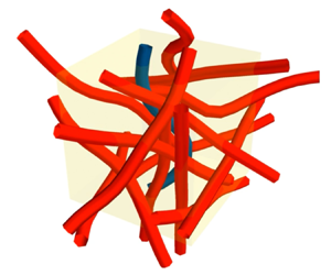
Producing the filament suspension follows a common and straightforward algorithm. We first place an undeformed swimmer (length $L=33a$) in the periodic domain. We then randomly seed (in position and orientation) $M$ undeformed filaments of length $L=33a$. This will inevitably lead to overlapping between filaments, which must be addressed before the simulation is run. For low filament volume fraction, $\phi < 5\,\%$, where $\phi = 4 {\rm \pi}a^3 L M / (3V\Delta L)$, overlap is resolved as part of the seeding process itself, where filaments are checked for overlap as they are seeded and the seed is rejected if overlap occurs. This is continued until all $M$ filaments are successfully introduced to the domain. For high volume fractions, $\phi > 5\,\%$, filaments are placed at random positions and orientations in the domain, regardless of any overlap. To remove overlap, the filaments are allowed to evolve under very short-ranged repulsive forces with segment mobility based on Stokes drag. The filaments are allowed to evolve until all overlap is removed and this final configuration is used as the initial condition for our simulations. An example of a suspension simulation initial condition for $\phi = 11.2\,\%$ is shown in figure 2(a).

Figure 2.

Filament suspension seeding. (a) Render of an unconnected suspension from § 3.1 in a yellow periodic box at 11.3 % volume concentration. (b) Diagram of filaments connected by springs at the node at $\boldsymbol {r}_1$, as used in § 4.1. (c) A render of one periodic cell of the connected network suspension highlighting the placement of the connecting nodes.

Suspension simulations are conducted using two values of the non-dimensional relative bending modulus, $K_B' := K_B/K_B^{swim} = 10^{-3}$ and $1$, where $K_B^{swim}$ is the bending modulus of the swimmer. These values correspond to relatively flexible and stiff networks, respectively. We use non-dimensional parameters in our study, allowing us to transcend a link to any specific organism and environment, but we briefly present dimensional measurements from the literature for context. For C. elegans, estimates of $K_B^{swim}$ range widely, from $O(10^{-16})$ to $O(10^{-13})\ \text {N m}^2$ (Fang-Yen et al. Reference Fang-Yen, Wyart, Xie, Kawai, Kodger, Chen, Wen and Samuel2010; Sznitman et al. Reference Sznitman, Purohit, Krajacic, Lamitina and Arratia2010; Backholm, Ryu & Dalnoki-Veress Reference Backholm, Ryu and Dalnoki-Veress2013). For mammalian sperm cells, the estimated range is at least $O(10^{-21})$ to $O(10^{-19})\ \text {N m}^2$ (Rikmenspoel Reference Rikmenspoel1965; Lindemann, Macauley & Lesich Reference Lindemann, Macauley and Lesich2005; Gadêlha Reference Gadêlha2012). Estimates for mucin fibres are scarce in the literature, partly due to significant variation in their diameter, which ranges from 3 to 10 nm (Shogren, Gerken & Jentoft Reference Shogren, Gerken and Jentoft1989). Given that $K_B$ scales with the fourth power of the diameter for long, thin tubes, this results in a variation spanning four orders of magnitude. Assuming a typical biopolymer Young's modulus of $1\ \mathrm {GPa}$, the estimated $K_B$ ranges from $O(10^{-25})$ to $O(10^{-22})\ \mathrm {N\ m}^2$.

Simulations are also performed for six different filament volume fractions between $\phi = 1.9\,\%$ and $18.9\,\%$. Videos of simulations with $\phi =7.6\,\%$ for both $K'_B=10^{-3}$ and $1$ are included in the supplementary material available at https://doi.org/10.1017/jfm.2024.603.

3.2. Swimming speeds in filament suspensions

We start by recording and measuring the swimming speed of the undulating filament as it moves through the filament suspensions. For each value of $K'_B$ and $\phi$, we perform 10 independent simulations, each with different randomly generated initial filament configurations, run for 20 periods of undulation. As the active filament swims, its stroke adds periodic contributions to the swimmer's speed. To remove these contributions, the swimming speed is defined as the period average of the centre of mass velocity in the direction of the period-averaged swimmer orientation (Kamal & Keaveny Reference Kamal and Keaveny2018).

At any given time $t$, the instantaneous velocity of the centre of mass of the swimmer is given by

(3.1)\begin{equation} \boldsymbol{V}_{CoM} = \frac{1}{N}\sum_{n=1}^N \boldsymbol{V}_n,\end{equation}

where $\boldsymbol {V}_n$ is the velocity of segment $n$. The instantaneous orientation vector of the swimmer is given by $\hat {\boldsymbol {p}} = \boldsymbol {p}/|\boldsymbol {p}|$ where

(3.2)\begin{equation} \boldsymbol{p} ={-}\frac{1}{N}\sum_{n=1}^N \hat{\boldsymbol{t}}_n,\end{equation}

and where $\hat {\boldsymbol {t}}_n$ is the tangent vector of segment $n$. We can then calculate the period-averaged velocity of the swimmer, $\boldsymbol {V}_{period}(t)$, for time $t\geq T$, as

(3.3)\begin{equation} \boldsymbol{V}_{period}(t) = \frac{1}{T}\int_{t-T}^{t}\boldsymbol{V}_{CoM}(t')\,{\mathrm d} t', \end{equation}

while the period-averaged orientation is $\hat {\boldsymbol {P}} = \boldsymbol {P}/|\boldsymbol {P}|$, where

(3.4)\begin{equation} \boldsymbol{P}(t) = \frac{1}{T}\int_{t-T}^{t}\hat{\boldsymbol{p}}(t')\,{\mathrm d} t'.\end{equation}

The swimming speed, $V_{swim}(t)$, at any given time is then defined as

(3.5)\begin{equation} V_{swim}(t) = \boldsymbol{V}_{period}(t)\boldsymbol{\cdot}\hat{\boldsymbol{P}}(t).\end{equation}

In figure 3(a), we present the normalised swimming speed $V_{swim}(t) / \langle V_{swim}^0 \rangle$, where $\langle V_{swim}^0 \rangle$ is the swimming speed in the absence of filaments, for each independent simulation, for increasing concentration and both values of the bending modulus. Along with this, we show in (b) of the same figure, $\langle V_{swim} \rangle /\langle V_{swim}^0 \rangle$, the average value of the swimming speed across both time and independent simulations. We see that in suspensions of relatively flexible filaments ($K'_B = 10^{-3}$), the speed of the swimmer is promoted up to 15 % due to the presence of the filaments, with more concentrated suspensions yielding higher speeds. For suspensions with stiffer filaments ($K'_B=1$), a small speed promotion of up to 5 % is observed at low concentrations, but at higher concentrations (above $\phi \sim 12\,\%$), the swimmer is on average hindered, displaying speed decreases of up to $20\,\%$.

Figure 3.

Swimmer speeds in the filament suspensions. (a) Superimposed swimmer speeds over 20 periods of undulation for 10 independent simulations for each parameter pair $(\phi, K'_B)$ in a filament suspension. (b) Mean swimming speed, averaged over time and simulations, for each filament stiffness, $K'_B$, as a function of filament volume fraction, $\phi$. Error bars signify $\pm 1$ standard deviation of simulations’ mean over time. (c) Mean of simulations’ standard deviation, $\sigma$, over time.

The speed enhancement at low concentrations is consistent with the speed increases of up to 20 % seen in simulations of 2-D undulatory swimmers in Stokes–Oldroyd-B viscoelastic fluids (Teran et al. Reference Teran, Fauci and Shelley2010; Thomases & Guy Reference Thomases and Guy2014). In common with the planar undulatory motion in Kamal & Keaveny (Reference Kamal and Keaveny2018), the average swimmer slowdown for rigid, concentrated networks is not due to a uniform speed decrease across all independent runs; instead, it is due to large variations in the speed, including periods of time where the swimmer is trapped within the network in some simulations. But in contrast, our speed enhancement is significantly less than in simulations of interrupted planar swimming, where fixed (Majmudar et al. Reference Majmudar, Keaveny, Zhang and Shelley2012) or tethered (Kamal & Keaveny Reference Kamal and Keaveny2018) discrete obstacles lead to three- to tenfold speed increases. We also see less enhancement than in helical swimming with fixed obstacles (at 40 %: Leshansky Reference Leshansky2009), where swimming speed can increase monotonically with concentration (Klingner et al. Reference Klingner, Mahdy, Hanafi, Adel, Misra and Khalil2020). We discuss mechanisms for these distinctions in § 6.

The fluctuations in the swimmer speed seen in figure 3(a) increase with concentration, but this effect is much larger for the stiffer networks. At the highest concentration, the swimmer is sometimes sped up by a factor of 2, but also sometimes forced backwards in a number of simulations. This is quantified by the standard deviation in panel (c) of the same figure, where the mean standard deviation, $\langle \sigma \rangle$, increases almost linearly with concentration and reaches $0.4$ of the unhindered swimmer speed in the most concentrated suspensions of stiff filaments.

4.1. Filament environment

A number of methods for generating linked filament networks exist in the literature. One approach, seen in 2-D (Head, Levine & MacKintosh Reference Head, Levine and MacKintosh2003a,Reference Head, Levine and MacKintoshb; DiDonna & Levine Reference DiDonna and Levine2006; Heussinger & Frey Reference Heussinger and Frey2006) and 3-D (Åström et al. Reference Åström, Kumar, Vattulainen and Karttunen2008) models of actin networks, is to seed straight filaments isotropically and add cross-links where filaments intersect, potentially removing loose ends (Wilhelm & Frey Reference Wilhelm and Frey2003; Huisman et al. Reference Huisman, van Dillen, Onck and Van der Giessen2007). Another option is to seed straight filaments, but let them grow into other shapes according to an algorithm, before forming cross-links (Buxton, Clarke & Hussey Reference Buxton, Clarke and Hussey2009).

Here, we use a probability-based algorithm to construct a phenomenological model of a generic network, based on Buxton & Clarke (Reference Buxton and Clarke2007). We place the swimmer, of length $L$, in the empty periodic domain and seed $N_{nodes}$ nodes randomly inside the domain at a distance at least $R_{min} = 2.2LN_{nodes}^{-1/3}$ from each other. The exponent of $-1/3$ corresponds to hard sphere packing inside a finite domain. For each pair of nodes, $i$ and $j$, with positions $\boldsymbol {r}_i$ and $\boldsymbol {r}_j$, respectively, we place a filament connecting these nodes with a probability $P_{conn}$ if the distance between nodes is $|\boldsymbol {r}_i - \boldsymbol {r}_j| = |\boldsymbol {r}_{ij}| < R_{max} = 1.2L$. The filament is placed along the vector $\boldsymbol {r}_{ij}$, with its centre at the midpoint of $\boldsymbol {r}_{ij}$ and formed of $N=\lfloor (r_{ij}-2r_{spacing})/\Delta L \rfloor$ segments, where $r_{spacing} = 2a$ is taken to ensure filaments do not overlap at the nodes. Linear spring forces $-k_s(x-\ell )\hat {\boldsymbol {x}}$, where $\boldsymbol {x}=x\hat {\boldsymbol {x}}$ is the end-to-end vector and $\ell$ is the natural spring length, are applied between all pairs of filament end segments that meet at a node. In doing this, we generate a network spanning the periodic domain with no external force holding it in place; in practice, the drag on the component filaments limits the network from moving as a rigid body. The seeding algorithm is summarised in figure 2(b).

To ensure that filaments do not overlap, this seeding procedure is carried out in a separate simulation, using friction-based mobility and an active collision barrier, until an equilibrium has been found. We once again define the volume concentration of the network by treating each segment as a sphere with its hydrodynamic radius $a$. That is, for $M$ filaments of length $L_i$ in a periodic domain with volume $V$, we have $\phi = 4 {\rm \pi}a^3 \sum _{i=1}^M{L_i} / (3V\Delta L)$. Under this definition, the concentration scales as the square of the number of nodes, $\phi \sim N_{nodes}^2$. Over a large number of independent random initial seeds, the concentration is normally distributed with a standard deviation that grows linearly with $N_{nodes}$.

Simulations are performed for different concentrations of filaments between $\phi = 3.4\,\%$ and $18.7\,\%$. We choose $N_{nodes}$ and $P_{conn}$ to produce networks of a given concentration with a common mean filament length of approximately $0.75L$, and common mean number of connections at each node (to within a reasonable tolerance). Our parameter choices are summarised in table 1.

Table 1.

Spring network seeding parameters for each concentration $\phi$, used in the algorithm in § 4.1.

The pair distribution function (PDF) of node separations under these configurations is displayed in figure 4(a). We see a bump near $R_{min}$ corresponding to close packing, but otherwise the PDF follows the shape for a uniform distribution, slightly enhanced. A render of one such network at 11.3 % volume concentration is shown in figure 2(c), with the nodes represented by black circles.

Figure 4.

Spring network seeding statistics. (a) Pair distribution function of node spacing for each of our concentrations, averaged over 1000 trials. The horizontal black dotted line corresponds to the pair distribution function of a uniform distribution in a periodic domain (Deserno Reference Deserno2004). (b) Histogram of the number of connections at each node for each of our concentrations, averaged over 100 trials. The mean in each case, represented by the vertical dotted line, is between 16 and 19.

Simulations are performed for two different values of the network filament bending modulus, $K'_B = 10^{-3}$ and $1$ (as for the filament suspensions), and for three values of the spring modulus, $k'_s = 0,0.36,3.6$, where $k'_s := k_sL^3/K_B^{swim}$. The swimmer bending and twist modulus remains constant, and the twist modulus, $K_T$, for every filament, is set equal to its bending modulus.

Simulations of flagellar swimming through a viscoelastic network formed of virtually cross-linked nodes by Wróbel et al. (Reference Wróbel, Lynch, Barrett, Fauci and Cortez2016) show that the connectivity number matters: higher-connectivity networks are stiffer. Here, we keep this number constant so that we can explore the effect of the other parameters in the system: the network filament bending modulus, the filament concentration and the spring modulus of the networks. The distribution of connection numbers in each case is shown in figure 4(b), where the mean connectivity number in each of our simulations is between 16 and 19. For comparison, cubic lattices with the diagonals excluded and included have connectivity numbers of 6 and 26, respectively, and were used in Wróbel et al. (Reference Wróbel, Lynch, Barrett, Fauci and Cortez2016). Buxton & Clarke (Reference Buxton and Clarke2007) use connectivity numbers between 5 and 15.

4.2. Swimming speeds in filament networks

We now present results from simulations examining swimmer motion in the connected filament networks. We again explore the effects of filament bending stiffness and volume fraction, but now also include the spring constant of the connections. For each triplet of parameters $(K'_B,\phi,k'_s)$, five simulations are performed, each with a different initial random configuration, and each running for 20 undulation periods.

The mean speed and standard deviation over the simulation run, $\langle V_{swim} \rangle$ and $\langle \sigma \rangle$, are presented in figure 5. We perform simulations for three different values of the spring constant. In the case where $k'_s=0$, the simulations differ from the filament suspensions in § 3 only in the seeding algorithm. For comparison, $\langle V_{swim} \rangle$ and $\langle \sigma \rangle$ from the suspension simulations are reproduced in this figure. We see that, for $k'_s=0$ and $0.36$, the trend in the data follows that found for filament suspension simulations: swimmer speed is promoted with concentration in flexible networks ($K'_B=10^{-3}$) up to $\sim 15\,\%$, but rigid networks ($K'_B=1$) produce a small speed promotion followed by a hindrance as concentration increases.

Figure 5.

Swimmer speeds in the filament networks. Mean normalised swimmer speed and standard deviation over 20 periods of undulation, as a function of the volume fraction of network filaments, for both values of the network filament bending modulus and for all three values of the network spring strength $k'_s$. Results for each parameter set are averaged from 5 independent simulations, and error bars signify $\pm 1$ standard deviation over the 5 simulations. For comparison, the suspension measurements from figure 3 are included in pale grey.

The more striking differences with the suspensions simulations are observed when $k'_s=3.6$, where the filament tethers are stiffer than the swimmer. Here, the swimmer speed in the flexible network decreases monotonically with concentration, down to an approximate reduction of $12\,\%$. The swimmer is hindered even further in the stiff filament network, with speeds decreasing by approximately $35\,\%$ at the highest concentrations. Interestingly, at intermediate concentrations, there is little difference with the weaker-spring scenarios. The effects of the stronger spring constant also yield considerably higher fluctuations in swimming speed with a standard deviation of up to $0.2\langle V_{swim}^0 \rangle$, although notably not as high as in the unconnected suspensions from § 3 where the standard deviation can be as high as $0.4 \langle V_{swim}^0 \rangle$.

5.1. The role of steric forces directly

The barrier force can result in a non-trivial net force on the swimmer that can push or pull it through the environment. We compute the mean period-averaged barrier force in the swimming direction, $\langle F_{swim} \rangle$. This can be measured analogously to $\langle V_{swim}\rangle$ in (3.1)–(3.5), namely

(5.1a–c)\begin{align} \boldsymbol{F}_{total} = \sum_{n=1}^N \boldsymbol{F}_n^B, \quad \boldsymbol{F}_{period}(t) = \frac{1}{T}\int_{t-T}^t\boldsymbol{F}_{total}(t')\,{\mathrm d} t', \quad F_{swim}(t) = \boldsymbol{F}_{period}(t)\boldsymbol{\cdot}\hat{\boldsymbol{P}}(t), \end{align}

noting that since the constraint forces on the swimmer sum to zero, the total barrier force is equal to the total hydrodynamic force, $\sum _n \boldsymbol {F}_n^B = \sum _n \boldsymbol {F}_n^H$.

The total force, $\langle F_{swim} \rangle$, in the suspensions is presented in figure 6(a). For all but the most concentrated case with the stiff filaments, the steric forces act against the direction of swimming. This is somewhat surprising as everywhere where this force is opposite the swimming direction, the velocity plot in figure 3 showed us that the swimmer is travelling faster than it does in the absence of filaments. The high-concentration, high-stiffness case appears an outlier, being pushed on average forwards, indicative of a different regime which will appear again in the spring networks.

Figure 6.

Force from the suspensions. While forces correlate with speed fluctuations, on average they push backwards (with the outlying high-$\phi$, high-$K'_B$ result indicative of a different regime we will also see in the spring networks). (a) Mean period-averaged force on the swimmer as a function of $\phi$, non-dimensionalised on the swimmer length and bending modulus. Error bars signify $\pm 1$ standard deviation over the 10 simulations. (b) Period-averaged force on the swimmer over time for the circled data point on the left, overlaid with the swimming velocity. Fluctuations in the force are seen to correlate with speed, but consider the region between the two horizontal bars: the swimmer speed often remains above the swimming speed in the absence of filaments (red line), despite the forces being negative, i.e. pushing backwards (orange line).

Although the direction of the mean force appears at odds with the increase in swimming speed, an examination of the time series before averaging shows a direct correlation between force and speed fluctuations, as shown in figure 6(b). But, still, the region between the horizontal lines in this panel represents times when the forces oppose swimming, and yet the swimmer is still travelling faster than it would in the absence of filaments, suggestive of a uniform promotion in speed across the simulation.

The filament networks follow similar trends but paint a more nuanced picture, with the total forces presented in figure 7. As in the suspensions, the steric forces from interactions with flexible network filaments push against the direction of swimming, with larger concentrations leading to stronger opposing forces. Once again, this happens despite the swimmer moving faster in these networks than they would at 0 % concentration (figure 5), although this is not universal: at the highest spring constant the filament speed does drop below its filament-free value. Interestingly, increasing the spring constant from $k'_s=0$ to $0.36$ makes little difference to the force yet mildly promotes swimming speed. At low filament concentrations, the swimmer behaves similarly in stiff and flexible filament networks, however, we see that above a critical concentration the forces from stiff networks will push in the direction of swimming yet the swimmer slows down. The force is much weaker for the $(k'_s=0, K'_B=1)$ case than in the matching suspension case, which we attribute to the differences in filament seeding. Increasing the spring constant recaptures and enhances the behaviour seen in the suspension.

Figure 7.

Forces from the spring networks: mean force on the swimmer in the swimming direction. Plotted as a function of the volume concentration of network filaments, for both values of the network filament bending modulus and all three spring constants. Results for each parameter set are averaged from 5 independent simulations. This is analogous to figure 6 in the filament suspensions.

These results suggest that there are two force regimes for the swimmer: one where the swimmer is gently resisted, almost linearly with concentration; and one where the swimmer is pushed forwards by the network. What is surprising is that these two force regimes do not clearly translate to observable swimming speed regimes. In particular, the barrier forces cannot be responsible for the speed increase seen in suspensions at lower-to-mid concentrations. We conclude that something else is acting to mask the total applied force.

5.2. The role of the swimming gait

Along with modifying the swimmer's rigid body motion, steric forces can also act to change the swimming gait. Swimmer undulations produce collisions with the surrounding filaments, inducing lateral forces which can reduce the amplitude of the undulation and alter the beat plane, making the gait less effective. Sample gaits from the suspension simulations, in both the beating and out-of-beating plane, are illustrated at increasing concentration in figure 8(a). These stills show that in flexible suspensions, increased concentration leads to slightly reduced beating-plane amplitudes and minor out-of-plane movements. But in rigid suspensions, especially at the highest concentration (bottom row), sample gaits deviate significantly from beating behaviour in a filament-free environment, with out-of-plane amplitude sometimes surpassing in-plane amplitude.

Figure 8.

Swimming gait amplitudes and effectiveness in suspensions. Higher concentrations lead to smaller-amplitude swimming gaits and slower swimming speeds. (a) Snapshots of sample swimming gaits, moving from left to right, in the beating plane (green, ‘side on’) and in the out-of-beating plane (purple, ‘top down’). Snapshots are from a suspension simulation and take place over two periods of undulation after a given time $t^*$. The mean amplitude in the swimming direction–beating plane, $A$, is marked with dotted black lines. As panel (b) summarises, the amplitude decreases as concentration increases, which coincides with deflection in the out-of-beating plane. This is emphasised when the suspended filaments are more rigid. Videos of the $\phi =7.6\,\%$ cases, with the surrounding filaments visible, are included in the supplementary material. (b) Mean amplitude in the beating plane, $\langle A \rangle$, for increasing concentration of suspension filaments, and for suspension filaments with bending modulus $K'_B=10^{-3}$ and $1$. The amplitude decreases with $\phi$. (c) Mean speed achieved with the extracted swimmer gait when placed in a 0 % concentration fluid, $\langle V_{swim}^{from\,gait}\rangle$, subject to no external forces, following the procedure in Appendix A. This correlates well with the amplitude graph to the left, and shows that the gait enforced by the filament suspension is less effective at swimming than the unrestricted gait in an empty fluid. In both (b) and (c), error bars signify $\pm 1$ standard deviation over the 10 simulations.

We can quantify these observations by measuring the mean amplitude in the beating plane, presented in figure 8(b) for suspensions and in figure 9(a) for our networks. We find that increased filament stiffness, $K'_B$, and for the networks, increased spring constants, $k'_s$, lead to smaller amplitudes at higher concentrations.

Figure 9.

Swimming gait amplitudes and effectiveness in networks. (a) Mean amplitude in the beating plane for increasing concentration of network filaments, and for network filaments with bending modulus $K'_B=10^{-3}$ and $1$ connected with springs with three different spring constants, $k'_s$. (b) Mean speed achieved with the extracted swimmer gait from the network simulations, following the procedure in Appendix A. This is the network analogue of figure 8. Combined with figure 7, this demonstrates that collectively, the gait and total barrier force, apart from in the most concentrated case with the stiffest filaments and spring constants, act to slow the swimmer down.

We can assess further the efficacy of these reduced-amplitude gaits by examining how well they propel the swimming in the absence of filaments. To do this, we remove the rigid body motion from the swimmer in the filament environment and recompute it in a viscous fluid absent of any filaments using the remaining undulations. We describe this computation in detail in Appendix A. The resulting speed when the imposed-gait swimmer swims is shown in figures 8(c) and 9(b). Correlating strongly with the stroke amplitude in both the suspensions and the networks, we see that the imposed gait is less effective at swimming, and increasingly so for the higher $K'_B$ and (in the network) higher $k'_s$. Thus, any gait changes result in reduced swimming speeds rather than the increases that we observe in the full simulations.

5.3. The role of hydrodynamics

So far we have seen that steric interactions, at mid-to-low concentrations, hinder swimming speed directly through rigid body forces. Additionally, when we remove all suspended filaments and impose the swimming gait seen in the full simulations, the swimmer again moves with a reduced speed compared with its natural gait in an empty fluid.

To understand the speed increases noted in figure 3, having eliminated steric forces and swimming gait, we turn our attention to hydrodynamic interactions. To investigate this, we run our suspension simulations again, including all filaments but now without hydrodynamic interactions between the suspended bodies. We accomplish this by solving the fluid mobility problem in (2.11) using a resistive force theory (RFT) (Johnson & Brokaw Reference Johnson and Brokaw1979; Lauga & Powers Reference Lauga and Powers2009) with coefficients tuned to recover the correct filament dynamics as in Schoeller & Keaveny (Reference Schoeller and Keaveny2018). The details are provided in Appendix B.

The resulting force and speed of the swimmer in these simulations without hydrodynamics are shown in figure 10 and, similar to the gait analysis simulations in figure 8, show no modest increase in speed at low-to-mid concentrations. Unlike simulations with full hydrodynamics (reproduced from figure 3 in light grey in the background of figure 10), we see that the swimming speed in this concentration regime is strongly affected by the steric forces, as evidenced by the strong correlation between these forces (a) and the resulting speed (b). At these concentrations, also observe the reduction in swimmer amplitude present in the full simulations, figure 8.

Figure 10.

Non-hydrodynamic simulations using RFT. In the absence of hydrodynamic interactions, the forces experienced by the swimmer strongly correlate to the swimmer speed. (a) Mean force on the swimmer in the swimming direction. (b) Mean normalised swimmer speed (with results from figure 3, which include hydrodynamic interactions, reproduced in the background in light grey for comparison). In both panels, results are again averaged from 20 periods of undulation and are plotted as a function of the volume concentration of network filaments, for both values of the network filament bending modulus. Results for each parameter set are averaged from 10 independent simulations, and error bars signify $\pm 1$ standard deviation over these simulations.

Although the general shape of the total force graph is similar between RFT and the full simulations, see figures 6 and 10, it is noticeable that the backwards force response of $K'_B=10^{-3}$ is stronger, and of $K'_B=1$ is weaker, without the hydrodynamics. This can be attributed to the difference in hydrodynamic model since, when the hydrodynamics is included, both the swimmer and the suspended filaments can deform each other without contact; whereas in the drag-based model, the filaments only affect each other on contact through the repulsive forces. In short, the presence of hydrodynamics in figure 3 significantly changes the swimmer behaviour from a steric force driven regime seen in the absence of hydrodynamics, in figure 10.

5.4. Summary of investigation

In this examination of swimmer motion, we have analysed the swimming gait and the forces experienced by the swimmer. While we find that the fluctuations in the swimming speed are closely correlated with collisions between the swimmer and filaments, enhancement in the mean speed is not linked to the force experienced by the swimmer or changes in swimming gait. In fact, both effects would produce a monotonic decrease in the speed with filament concentration. This suggests that the enhancement is instead linked to hydrodynamic interactions between the swimmer and filaments. We confirm this by performing RFT simulations where hydrodynamic interactions between the swimmer and filaments are removed and for which we do not observe any enhanced speed.