


1. Introduction
We investigate the propagation of three-dimensional (3-D) hydraulic fractures emerging from a point source accounting for buoyancy forces. Hydraulic fractures (HFs) are tensile fluid-filled fractures propagating under internal fluid pressure that exceed the minimum compressive in situ stress of the surrounding media (Detournay Reference Detournay2016). They are encountered in various engineering applications (Germanovich & Murdoch Reference Germanovich and Murdoch2010; Jeffrey et al. Reference Jeffrey, Chen, Mills and Pegg2013; Smith & Montgomery Reference Smith and Montgomery2015), but also occur in nature due to fluid over-pressure at depth, for example during the formation of magmatic intrusions (Spence, Sharp & Turcotte Reference Spence, Sharp and Turcotte1987; Lister & Kerr Reference Lister and Kerr1991; Rivalta et al. Reference Rivalta, Taisne, Bunger and Katz2015). The minimum physical ingredients to model HF growth are lubrication flow within the elastically deformable fracture coupled with quasi-static fracture propagation under the assumption of linear elastic fracture mechanics (LEFM) (Detournay Reference Detournay2016). In the absence of buoyancy, theoretical predictions reproduce well experiments in brittle and impermeable materials (Bunger & Detournay Reference Bunger and Detournay2008; Lecampion et al. Reference Lecampion, Desroches, Jeffrey and Bunger2017; Xing et al. Reference Xing, Yoshioka, Adachi, El-Fayoumi and Bunger2017).
Hydraulic fractures propagate radially from a point source and continue so in the absence of buoyancy. For such a geometry, the growth is initially dominated by energy dissipation in viscous flow and transitions to a regime dominated by fracture energy dissipation at late time (in association with the increase of the fracture perimeter). Growth solutions in both regimes are well known (Abé, Keer & Mura Reference Abé, Keer and Mura1976; Spence & Sharp Reference Spence and Sharp1985; Savitski & Detournay Reference Savitski and Detournay2002). The presence of buoyant forces necessarily elongates the fracture. A large body of work investigated the impact of buoyant forces on two-dimensional (2-D) plane strain fractures (Weertman Reference Weertman1971; Spence & Turcotte Reference Spence and Turcotte1985, Reference Spence and Turcotte1990; Spence et al. Reference Spence, Sharp and Turcotte1987; Lister Reference Lister1990a; Roper & Lister Reference Roper and Lister2007). The early work of Weertman (Reference Weertman1971) focused on a toughness-dominated fracture with a linear pressure gradient, and did not consider any fluid flow. These considerations led to a fluid-filled pocket with a stress intensity factor equal to the material resistance at the upper tip, and zero at the lower tip, of such a bubble crack. A 2-D pulse is hence created. Owing to the lack of coupling with lubrication flow, a description of the dynamics of its ascent is missing. A first attempt to include viscous effects was made by Spence et al. (Reference Spence, Sharp and Turcotte1987) and Spence & Turcotte (Reference Spence and Turcotte1990). Lister (Reference Lister1990a) has obtained solutions as a function of a dimensionless fracture toughness with a focus on small fracture toughness / large viscosity cases. These 2-D buoyant HFs exhibit a distinct head region, close to the propagating edge, where a hydrostatic gradient develops, and a tail region where viscous flow occurs within a conduit of constant width. The solution in the so-called toughness-dominated regime was obtained by Roper & Lister (Reference Roper and Lister2007), complementing earlier work (Lister Reference Lister1990a; Lister & Kerr Reference Lister and Kerr1991).
A pseudo-three-dimensional (pseudo-3-D) solution for viscosity-dominated buoyant fractures was developed by Lister (Reference Lister1990b) in conjunction with a scaling analysis. Assuming a large aspect ratio for the fracture allows for a partial uncoupling of elasticity and lubrication flow. The boundary conditions of his model are such that the fracture has an unprescribed open upper end, such that this approximate solution is deemed to be valid in the near-source region. It predicts an ever-increasing horizontal extent of the fracture, which must be limited in the case of a finite, non-zero fracture toughness. A planar 3-D solution has been derived by Garagash & Germanovich (Reference Garagash and Germanovich2014) (see also Germanovich et al. Reference Germanovich, Garagash, Murdoch and Robinowitz2014; Garagash & Germanovich Reference Garagash and Germanovich2022) in the limit of large material toughness. This approximate solution is constructed by matching a constant-breadth (blade-like) viscosity-dominated tail with a 3-D toughness-dominated head under a hydrostatic gradient. This approximate toughness solution shows a propagating head akin to a constant 3-D Weertman pulse (Weertman Reference Weertman1971) propagating upwards due to the linear extension of a fixed breadth in a viscosity-dominated tail. Recently, the problem of a finite volume release has been investigated in the limit of zero fluid viscosity numerically by Davis, Rivalta & Dahm (Reference Davis, Rivalta and Dahm2020), focusing on the minimal volume required for the start of buoyant propagation. Similar simulations are reported in Salimzadeh, Zimmerman & Khalili (Reference Salimzadeh, Zimmerman and Khalili2020), where lubrication flow is included but only small-volume releases are investigated, without an extensive study of the late-time growth of buoyant 3-D HFs.
In this paper, we investigate the transition of initially radial expansion HFs to the late-time fully 3-D buoyant regimes accounting for the complete coupling between elastohydrodynamic lubrication flow and LEFM. Notably, we aim to clarify the domain of validity of previous contributions in the viscosity- and toughness-dominated limits, and fully understand the solution space of 3-D buoyant fractures under constant-volume release.
2. Formulation and methods
2.1. Mathematical formulation
We consider a pure opening mode (mode I) HF propagating from a point source located at depth in the  $x$–
$x$– $z$ plane, as sketched in figure 1. This
  $x$–
$x$– $z$ plane is perpendicular to the minimum in situ stress
  $\sigma _{o}(z)$ (taken positive in compression). We assume that the minimum in situ stress acts in the
  $y$ direction and is thus perpendicular to the gravity vector
  ${\boldsymbol {g}=(0,0,-g)}$ (with
  ${g}$ the Earth's gravitational acceleration). Owing to the possibly large fracture dimensions, we account for a linear vertical gradient of the in situ stress (resulting from the initial solid equilibrium). Assuming a linear elastic medium with uniform properties, the quasi-static balance of momentum for a planar tensile HF reduces to a hyper-singular boundary integral equation over the fracture surface
  $\mathcal {A}(t)$. This integral equation relates the fracture width
  ${w(x,z,t)}$ to the net loading, which is equivalent to the difference between the fluid pressure inside the fracture
  ${p_{f}(x,z,t)}$ and the minimum compressive in situ stress
  ${\sigma _{o}(x,z)}$ (Crouch & Starfield Reference Crouch and Starfield1983; Hills et al. Reference Hills, Kelly, Dai and Korsunsky1996):
 \begin{equation} p(x,z,t)=p_{f}(x,z,t)-\sigma_{o}(x,z)={-}\frac{E^{\prime}}{8{\rm \pi}} \int_{\mathcal{A}(t)}\frac{w(x^{\prime},z^{\prime},t)}{[(x^{\prime}-x)^{2}+ (z^{\prime}-z)^{2}]^{3/2}}\,\text{d}x^{\prime}\,\text{d}z^{\prime},\end{equation}
where  $E^{\prime }=E/(1-\nu ^{2})$ is the plane-strain modulus, with
  $E$ the material Young's modulus and
  $\nu$ its Poisson's ratio. As typically observed in the Earth's crust (Jaeger, Cook & Zimmerman Reference Jaeger, Cook and Zimmerman2007; Cornet Reference Cornet2015; Heidbach Reference Heidbach2018), the minimum confining stress
  ${\sigma _{o}(z)}$ increases linearly with depth proportional to the solid weight
  ${\gamma _{s}=\rho _{s}g}$ multiplied by a dimensionless lateral Earth pressure coefficient
  ${\alpha }$. Accounting for the downward orientation of the gravitational vector in the chosen coordinate system (see figure 1), the vertical gradient for
  ${\sigma _{o}(z)}$ is linear over the entire medium:
 \begin{equation} \text{d}\sigma_{o}(z)/\text{d}z={-}\alpha\rho_{s}g\to \boldsymbol{\nabla}\sigma_{o}=\alpha\rho_{s}\boldsymbol{g}. \end{equation}
Fluid flow within the thin deforming fracture is governed by lubrication theory (Batchelor Reference Batchelor1967). Neglecting any fluid exchange between the rock and the fracture (a reasonable assumption for tight formations and high-viscosity fluids), the width-averaged continuity equation for an incompressible fluid reduces to
 \begin{equation} \frac{\partial w(x,z,t)}{\partial t}+\boldsymbol{\nabla}\boldsymbol{\cdot}\left(w(x,z,t)\, \boldsymbol{v}_{f}(x,z,t)\right)=\delta(x)\,\delta(z)\,Q_{o}(t),\end{equation}
where  $\boldsymbol {v}_{f}(x,z)$ is the width-averaged fluid velocity, and
  $Q_{o}$ is the volumetric flow rate at the point source located at the origin
  ${(x,z)=(0,0)}$. Additionally, the assumption of no fluid exchange with the surrounding medium dictates that the total volume of the fracture is equal to the total volume released. Assuming a constant release rate
  $Q_{o}$, the global volume conservation is
 \begin{equation} \mathcal{V}(t)=\int_{\mathcal{A}(t)}w(x,z)\,\text{d}x\,\text{d}z=Q_{o}t.\end{equation}
Assuming laminar flow and a Newtonian rheology, the fluid flux  $\boldsymbol {q}(x,z,t)=w(x,z,t)$
  $\boldsymbol {v}_{f}(x,z,t)$ reduces to Poiseuille's law accounting for buoyancy forces:
 \begin{equation} \boldsymbol{q}(x,z,t)=w(x,z,t)\,\boldsymbol{v}_{f}(x,z,t)={-}\frac{w(x,z,t)^{3}}{\mu^{\prime}}\left(\boldsymbol{\nabla}p_{f} (x,z,t)-\rho_{f}\boldsymbol{g}\right),\end{equation}
where  $\mu ^{\prime }=12\mu _{f}$ is the equivalent parallel plates fluid viscosity,
  $\mu _{f}$ is the fluid viscosity, and
  $\rho _{f}$ is the fluid density. Introducing the net pressure
  ${p(x,z,t)=p_{f}(x,z,t)-\sigma _{o}(z)}$ and using (2.2), (2.5) is rewritten as
 \begin{equation} \boldsymbol{q}(x,z,t)={-}\frac{w(x,z,t)^{3}}{\mu^{\prime}} \left(\boldsymbol{\nabla}p(x,z,t)+{\rm \Delta}\gamma\, \frac{\boldsymbol{g}}{\left|\boldsymbol{g}\right|}\right),\end{equation}
where  ${{\rm \Delta} \gamma ={\rm \Delta} \rho \,g=(\alpha \rho _{s}-\rho _{f})g}$ is the effective buoyancy contrast of the system. For
  $\alpha = 1$, it equals the buoyancy contrast between the solid and the fluid. Values of the lateral Earth pressure coefficient
  ${\alpha }$ different from 1 have no influence other than affecting the value of the effective buoyancy contrast
  ${{\rm \Delta} \gamma }$ of the system. We consider HFs at depth such that the confining stress is assumed to be sufficiently large for the presence of a fluid lag to be negligible (see discussion in Garagash & Detournay Reference Garagash and Detournay2000; Lecampion & Detournay Reference Lecampion and Detournay2007; Detournay Reference Detournay2016). In this limit, the boundary conditions at the fracture front reduce to a zero fluid flux normal to the front (
 ${\boldsymbol {q}(x_{c},z_{c})=0}$) and zero fracture width (
 ${w(x_{c},z_{c})=0}$) (see Detournay & Peirce (Reference Detournay and Peirce2014) for a detailed discussion).
Schematic of a buoyancy-driven hydraulic fracture (red for head, green for tail, grey for source region). The tail length is reduced for illustration, indicated by dashed lines and a shaded area. The fracture propagates in the  $x$–
$x$– $z$ plane with a gravity vector
  ${\boldsymbol {g}}$ oriented in the
  ${-z}$ direction. The fracture front
  ${\mathcal {C}(t)}$, fracture surface
  ${\mathcal {A}(t)}$ (dark grey area), opening
  ${w(x,z,t)}$, net pressure
  ${p(x,z,t)}$, and local normal velocity of the fracture
  ${v_{c}(x_{c},z_{c})}$ with
  ${(x_{c},z_{c})\in {\mathcal {C}(t)}}$ characterize fracture growth under a constant release rate
  ${Q_{o}}$ in a medium with a linear confining stress with depth
  ${\sigma _{o}(z)}$. Here,
  ${\ell ^{{head}}(t)}$ and
  ${b^{{head}}(t)}$ denote the length and breadth of the head,
  ${\ell (t)}$ is the total fracture length, and
  ${b(z,t)}$ is the local breadth of the fracture.

Finally, the fracture is assumed to propagate in quasi-static equilibrium under the assumption of LEFM. For a pure opening mode fracture, the propagation criterion reduces to
 \begin{equation} \left(K_{I}(x_{c},z_{c})-K_{Ic}\right)v_{c}(x_{c},z_{c})=0,\quad v_{c}(x_{c},z_{c})\ge0,\quad K_{I}(x_{c},z_{c})\le K_{Ic},\end{equation}
for all  ${(x_{c},z_{c})\in {\mathcal {C}(t)}}$. In this equation,
  ${K_{I}}$ is the stress intensity factor,
  ${K_{Ic}}$ is the material fracture toughness, and
  ${v_{c}(x_{c},z_{c})}$ is the local fracture velocity normal to the front (see figure 1). When the fracture is propagating at a point
  ${(x_{c},z_{c})}$, the velocity is positive, and the stress intensity factor equals the material toughness (
 ${v_{c}(x_{c},z_{c})>0}$,
  $K_{I}(x_{c},z_{c})=K_{Ic}$).
2.2. Numerical solver
For the numerical solution of the moving boundary problem presented in § 2.1, we use the open-source 3-D-planar HF solver PyFrac (Zia & Lecampion Reference Zia and Lecampion2020). This solver is based on the implicit level set algorithm (ILSA) developed originally by Peirce & Detournay (Reference Peirce and Detournay2008) for 3-D planar HFs (see also Dontsov & Peirce (Reference Dontsov and Peirce2017) for more details). The numerical scheme combines the discretization of a finite domain with the steadily moving plane-strain HF asymptotic solution (Garagash, Detournay & Adachi Reference Garagash, Detournay and Adachi2011) near the fracture front. Even with a coarse discretization of the finite domain, the coupling between these two scales allows for an accurate estimation of the fracture front velocity  $v_{c}(x_{c},z_{c})$. We use the improvement of Peruzzo, Lecampion & Zia (Reference Peruzzo, Lecampion and Zia2021), which imposes strict continuity of the fracture front during its reconstruction from the level set values at the cell centre. The discretization of the elasticity equation (2.1) is performed using piecewise constant rectangular displacement discontinuity elements, while an implicit finite volume scheme is used for elastohydrodynamic lubrication flow. In various implementations, this numerical scheme has proved to be both accurate and robust when tested against known HF growth solutions (Peirce Reference Peirce2015, Reference Peirce2016; Zia, Lecampion & Zhang Reference Zia, Lecampion and Zhang2018; Moukhtari, Lecampion & Zia Reference Moukhtari, Lecampion and Zia2020; Zia & Lecampion Reference Zia and Lecampion2020; Möri & Lecampion Reference Möri and Lecampion2021).
We use a minimal initial discretization of  $61\times 61$ elements, and add elements as the fracture elongates for all simulations presented herein. Our simulations need to run over several orders of magnitude in time and space to capture the transition and the late-time buoyant propagation stage. We thus adopt two different remeshing techniques to ensure that the smaller spatial dimension (horizontal in our case) always satisfies a minimum discretization of
  ${61}$ elements. A second condition of the discretization is that the original element aspect ratio is ensured during the entire simulation, even when the aspect ratio of the mesh domain is changing. This discretization constrains the maximum relative error on the fracture radius to 2–3 % for radial fractures (Zia & Lecampion Reference Zia and Lecampion2020; Möri & Lecampion Reference Möri and Lecampion2021). The fracture is initialized as a radial HF in the viscosity-dominated regime (Savitski & Detournay Reference Savitski and Detournay2002), which corresponds to the early-time solution of this type of fracture. We use this technique to ensure that we capture consistently the entire propagation in all the different regimes.
2.3. Scaling analysis
In the configuration studied herein, the HF initially propagates radially outwards from a point source. It remains radial as long as the fracture is sufficiently small that buoyancy forces remain negligible. At late time, the fracture elongates in the direction of the buoyant force. A head and tail structure similar to the plane-strain (2-D) case is expected to develop. This head–tail structure has either a horizontal breadth that stabilizes in space at late times, or an ever-growing one (Lister Reference Lister1990b; Garagash & Germanovich Reference Garagash and Germanovich2014). We capture the evolution of the fracture shape by introducing  ${\ell (t)}$ as the vertical extent (to which we will alternatively refer as the fracture length) and
  ${b(z,t)}$ as the horizontal breadth (see figure 1). We recognize that the horizontal breadth may not be uniform in space and will thus refer to
  ${b(t)}$ as the maximum horizontal breadth of the fracture. We scale these fracture dimensions as
 \begin{equation} \ell(t)=\ell_{*}(t)\,\gamma(\mathcal{P}_{i}),\quad b(t)=b_{*}(t)\, \beta(\mathcal{\mathcal{P}}_{i}),\end{equation}
where  ${\ell _{*}(t)}$ and
  ${b_{*}(t)}$ are a characteristic fracture length and (maximum) breadth, respectively, and
  ${\gamma }$ and
  ${\beta }$ are the corresponding dimensionless extents. Following the notation of previous work (Detournay Reference Detournay2004), we scale the fracture width and net pressure as
 \begin{equation} w(x,z,t)=w_{*}(t)\,\varOmega (x/b_{*},z/\ell_{*},\mathcal{\mathcal{P}}_{i}),\quad p(x,z,t)=p_{*}(t)\,\varPi(x/b_{*},z/\ell_{*},\mathcal{\mathcal{P}}_{i}),\end{equation}
with  ${w_{*}(t)}$ and
  ${p_{*}(t)}$ the characteristic width and net pressure scales,
  ${\varOmega }$ and
  ${\varPi }$ the dimensionless width and pressure. In the previous expressions, we recognized that the characteristic scales may depend on time and that the dimensionless solution is a function of a finite set of dimensionless numbers
  $\mathcal {P}_{i}$.
Introducing such a scaling into the governing equations provides a set of dimensionless groups denoted by  ${\mathcal {G}}$. In particular, the scaling of the elasticity equation (2.1) provides, besides the characteristic aspect ratio of the fracture,
 \begin{equation} {\mathcal{G}_{s}=b_{*}/\ell_{*}}, \end{equation}
a dimensionless group defined as the ratio between the characteristic elastic pressure  $w_{*}E^{\prime }/b^{*}$ and the characteristic net pressure
  $p_{*}$:
 \begin{equation} \mathcal{G}_{e}=\frac{w_{*}E^{\prime}}{p_{*}b_{*}}.\end{equation}
Elasticity is always of first order for a fracture problem (i.e.  $\mathcal {G}_{e}=1$), such that this equation yields a direct relation between the characteristic net pressure, fracture opening, and a fracture dimension. Scaling wise, the global volume conservation (2.4) provides a ratio between the released volume
  ${Q_{o}t}$ and the characteristic fracture volume
  ${w_{*}b_{*}\ell _{*}}$:
 \begin{equation} \mathcal{G}_{v}=\frac{Q_{o}t}{w_{*}b_{*}\ell_{*}}.\end{equation}
A dimensionless fracture toughness  ${\mathcal {G}_{k}}$ emerges from the linear fracture propagation criterion
  $K_{I}=K_{Ic}$ as a ratio between the characteristic LEFM pressure for the material
  ${K_{Ic}/\sqrt {b_{*}}}$ and the characteristic net pressure
  ${p_{*}}$:
 \begin{equation} \mathcal{G}_{k}=\frac{K_{Ic}}{p_{*}\sqrt{b_{*}}}.\end{equation}
Poiseuille's viscous drop (2.6) inside the fracture provides a dimensionless group akin to a dimensionless viscosity defined as the ratio between the characteristic viscous pressure  ${\mu ^{\prime }Q_{o}/w_{*}^{3}}$ and the characteristic pressure
  ${p_{*}}$:
 \begin{equation} \mathcal{G}_{m}=\frac{\mu^{\prime}Q_{o}}{w_{*}^{3}p_{*}}.\end{equation}
Finally, a last dimensionless group relates the characteristic buoyancy pressure  ${{\rm \Delta} \gamma \,\ell _{*}}$ to the characteristic pressure
  $p_{*}$:
 \begin{equation} \mathcal{G}_{b}=\frac{{\rm \Delta}\gamma\,\ell_{*}}{p_{*}}.\end{equation}
Using these dimensionless groups to emphasize the relative importance of the underlying physical mechanism, one obtains different scalings associated with different propagation regimes.
3. Onset of the buoyant regime
The contribution of buoyant forces is negligible for a small enough fracture: from (2.15),  $\mathcal {G}_{b}\ll 1$. In the absence of buoyancy, the HF propagates with a radial penny-shaped geometry. In an impermeable medium, Savitski & Detournay (Reference Savitski and Detournay2002) have shown that the HF transitions from a viscosity-dominated regime at early time towards a toughness-dominated regime at late time. The increase in fracture energy dissipation is related directly to the increase of the fracture perimeter. Self-similar solutions have been obtained in both the
  ${{M}}$ (viscous) scaling and the
  ${{K}}$ (toughness) scaling. Following Savitski & Detournay (Reference Savitski and Detournay2002), the characteristic scales are denoted with a subscript
  ${m}$ for the
  ${{M}}$ (viscous) scaling, and
  ${k}$ for the
  ${{K}}$ (toughness) scaling (see table 3 in the Appendix). The transition from the early-time viscosity-dominated to the toughness-dominated regime is captured entirely by a dimensionless toughness
  ${\mathcal {K}_{m}}$ increasing with time as (Savitski & Detournay Reference Savitski and Detournay2002)
 \begin{equation} {\mathcal{K}_{m}=K_{Ic}\,\frac{t^{1/9}}{E^{\prime13/18}Q_{o}^{1/6}\mu^{\prime5/18}}}.\end{equation}
This dimensionless toughness (defined in the  ${{M}}$ scaling) is directly related to a dimensionless viscosity defined in the
  ${{K}}$ scaling:
 \begin{equation} \mathcal{M}_{k}=\mathcal{K}_{m}^{{-}18/5}=\left(t_{mk}/t\right)^{2/5}.\end{equation}
In the absence of buoyancy, the toughness-dominated regime is reached when  ${\mathcal {K}_{m}\sim \mathcal {M}_{k}\sim 1}$ (Savitski & Detournay Reference Savitski and Detournay2002) (note our use of the fracture toughness
  $K_{Ic}$ instead of the reduced fracture toughness used in some previous work,
  $K^{\prime }=\sqrt {32/{\rm \pi} }\,K_{Ic}$), or alternatively for times greater than a characteristic time
  ${t_{mk}}$ defined as the time when
  ${\mathcal {K}_{m}=\mathcal {M}_{k}=1}$:
 \begin{equation} t_{mk}=\frac{E^{\prime13/2}\mu^{\prime5/2}Q_{o}^{3/2}}{K_{Ic}^{9}}.\end{equation}
The corresponding characteristic fracture radius at this time of transition between viscous and toughness growth is, according to Savitski & Detournay (Reference Savitski and Detournay2002),
 \begin{equation} \ell_{mk}=\frac{E^{\prime3}Q_{o}\mu^{\prime}}{K_{Ic}^{4}}.\end{equation}
To estimate when the buoyancy forces will start to play a role, still assuming that  ${b_{*}\sim \ell _{*}}$ – a hypothesis valid at the onset of the buoyant regime – it is worth computing the dimensionless buoyancy
  $\mathcal {G}_{b}$ from (2.15):
 \begin{equation} {\mathcal{B}_{m}={\rm \Delta}\gamma\,\frac{Q_{o}^{1/3}t^{7/9}}{E^{\prime5/9}\mu^{\prime4/9}},\quad \mathcal{B}_{k}={\rm \Delta}\gamma\,\frac{E^{\prime3/5}Q_{o}^{3/5}t^{3/5}}{K_{Ic}^{8/5}}}\end{equation}
in the viscous (subscript  $m$) and toughness (subscript
  $k$) scaling, respectively. As expected, the effect of buoyancy increases with time as the fracture grows. For each limiting regime, we deduce a transition time scale where buoyancy becomes dominant as the time when
  $\mathcal {B}_{m}$ (respectively
  $\mathcal {B}_{k}$) equals 1:
 \begin{equation} {t_{m\hat{m}}=\frac{E^{\prime5/7}\mu^{\prime4/7}}{{\rm \Delta}\gamma^{9/7}\,Q_{o}^{3/7}},\quad t_{k\hat{k}}=\frac{K_{Ic}^{8/3}}{E^{\prime}Q_{o}\,{\rm \Delta}\gamma^{5/3}}}.\end{equation}
In the following, we use  ${\hat {\cdot }}$ to highlight scalings where buoyancy plays a dominant role. Similarly to the previous viscosity to toughness transition, it is practical to obtain the corresponding transition length scales (see table 4 in the Appendix for details):
 \begin{equation} {\ell_{m\hat{m}}=\frac{E^{\prime3/7}Q_{o}^{1/7}\mu^{\prime1/7}}{{\rm \Delta}\gamma^{4/7}},\quad \ell_{k\hat{k}}=\frac{K_{Ic}^{2/3}}{{\rm \Delta}\gamma^{2/3}}\equiv\ell_{b}.}\end{equation}
It is worth noting that the toughness–buoyancy length scale  ${\ell _{k\hat {k}}}$ – that we will refer to alternatively as
  $\ell _{b}$ – can be obtained directly by assuming
  ${b_{*}\sim \ell _{*}}$ and balancing the toughness pressure
  ${K_{Ic}/\sqrt {\ell _{*}}}$ with the buoyancy pressure
  ${{\rm \Delta} \gamma \,\ell _{*}}$. Such a buoyancy length scale
  $\ell _{b}$ is strictly equal to the one obtained in the 2-D plane-strain case (Weertman Reference Weertman1971; Lister Reference Lister1990a; Lister & Kerr Reference Lister and Kerr1991; Heimpel & Olson Reference Heimpel and Olson1994; Roper & Lister Reference Roper and Lister2007) as well as for a finger-like 3-D geometry (Garagash & Germanovich Reference Garagash and Germanovich2014). The buoyancy effect becomes of order one either when the initially radial HF is still propagating in the viscosity-dominated regime (which implies
  $\mathcal {K}_m(t=t_{m\hat {m}}) < 1$; see (3.1)) or when it is already in the toughness-dominated regime (for which
  $\mathcal {M}_k(t=t_{k\hat {k}}) < 1$; see (3.2)). The interplay between the radial transition from viscosity- to toughness-dominated and the one from radial to buoyant can thus be captured by either
 \begin{equation} \mathcal{K}_{\hat{m}}=\mathcal{K}_m(t = t_{m\hat{m}})= \frac{K_{Ic}}{E^{\prime 9/14} Q_o^{3/14}\,{\rm \Delta}\gamma^{1/7}\,\mu^{\prime 3/14}} = \left(\frac{\ell_{m\hat{m}}}{ \ell_{mk}} \right)^{1/4} = \left(\frac{t_{m\hat{m}}}{t_{mk}} \right)^{1/9} \end{equation}
or
 \begin{equation} \mathcal{M}_{\hat{k}}=\mathcal{M}_k(t = t_{k\hat{k}})=\mu^{\prime}\, \frac{Q_{o}E^{\prime3}\,{\rm \Delta}\gamma^{2/3}}{K_{Ic}^{14/3}}=\frac{\ell_{mk}}{\ell_{k\hat{k}}} = \left(\frac{t_{mk}}{t_{k\hat{k}}} \right)^{2/5}. \end{equation}
These two dimensionless numbers are related as  $\mathcal {M}_{\hat {k}}^{-3/14}=\mathcal {K}_{\hat {m}}$. In fact, the different transition time scales (3.6a,b) and (3.3) are related as
  $t_{m\hat {m}}/t_{mk} =(t_{k\hat {k}}/t_{mk})^{27/35}$. The transition to buoyancy can therefore be grasped by any ratio of these transition time scales such that only one of the two parameters of (3.8) and (3.9) is required to define the transition.
In the following, we choose  $\mathcal {M}_{\hat {k}}$ to quantify the transition from a radial to a buoyant HF. Physically,
  $\mathcal {M}_{\hat {k}}$ quantifies if the fracture is viscosity-dominated (
 ${\mathcal {M}_{\hat {k}}>1}$) or toughness-dominated (
 ${\mathcal {M}_{\hat {k}}<1}$) at the onset of the buoyant regimes. Interestingly,
  $\mathcal {M}_{\hat {k}}$ is directly the ratio of the characteristic viscous–toughness transition length scale
  $\ell _{mk}$ (without buoyancy) with the buoyant toughness transition scale
  $\ell _{b}=\ell _{k\hat {k}}$. This confirms that
  $\mathcal {M}_{\hat {k}}$ in (3.9) captures properly the competition between the transition from viscous to toughness growth, and the transition to the buoyant regime.
4. Toughness-dominated buoyant fractures ( $\mathcal {M}_{\hat {k}}\ll 1$)

We first focus on toughness-dominated buoyant fractures ( $\mathcal {M}_{\hat {k}}\ll 1$), for which the transition to the buoyant regime occurs when the initially radial fracture is already propagating in the toughness-dominated regime (
 $t_{k\hat {k}}\gg t_{mk}$). Figures 2(e–i) show the complete fracture evolution for a value of
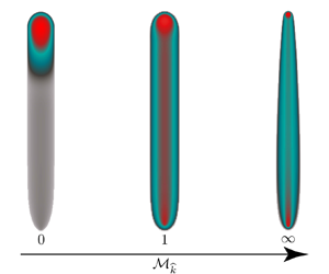
  ${\mathcal {M}_{\hat {k}}\approx 1.0\times 10^{-3}}$. The fracture is initially radial (figure 2e), elongates as buoyancy commences to act (figure 2 f,g), and ends-up being akin to a finger-like fracture (figure 2h,i). It is worth noting that for
  $t>t_{k\hat {k}}$, the breadth is uniform such that the creation of new fracture surfaces only occurs in the head region. This buoyant fracture exhibits a head-tail structure qualitatively similar to the plane-strain 2-D case (Lister Reference Lister1990a; Roper & Lister Reference Roper and Lister2007). In the tail, the breadth is constant, and no new fracture surfaces are created in the horizontal direction. This can be clearly observed from figure 2 (footprints i–h and the evolution of the breadth). In other words, the head is toughness-dominated, while in the tail only a viscous vertical flow is dissipating energy.
Toughness-dominated buoyant fracture. Green dashed lines indicate the 3-D  $\hat {{K}}$ GG (2014) solution. (a) Opening along the centreline
  ${w(0,z,t)/w_{\hat {k}}^{{head}}}$ for a simulation with
  ${\mathcal {M}_{\hat {k}}=1\times 10^{-2}}$. (b) Net pressure along the centreline
  ${p(0,z,t)/p_{\hat {k}}^{{head}}}$ for the same simulation. (c) Fracture length
  ${\ell (t)/\ell _{b}}$ for three simulations with large toughness
  ${\mathcal {M}_{\hat {k}}\in [10^{-3},10^{-1}]}$. Dash-dotted green lines highlight the late-time linear term of the
  ${\hat {{K}}}$ solution. (d) Fracture breadth
  ${b(t)/\ell _{b}}$ (continuous) and head breadth
  ${b^{{head}}(t)/\ell _{b}}$ (dashed). Grey lines indicate an error margin of
  ${5\,\%}$. (e–i) Evolution of the fracture footprint from radial (e) towards the final finger-like shape (h,i) for a fracture with
  ${\mathcal {M}_{\hat {k}}=1\times 10^{-3}}$. For the fracture shape in (i), the vertical extent is cropped between
  ${\ell (t)/\ell _{b}=6}$ and
  ${\ell (t)/\ell _{b}=30}$. Thick red dashed lines indicate the head shape according to the 3-D
  $\hat {{K}}$ GG (2014) solution. Note that the final stage (i) has not reached the constant terminal velocity (see c).

4.1. Toughness-dominated head
The characteristic scales of the toughness-dominated head are such that  $b_{*}^{{head}}\sim \ell _{*}^{{head}}$ and can be obtained assuming that toughness, buoyancy and elasticity are all of first order in the head. One obtains the head scales
 \begin{equation} \left.\begin{gathered} b_{\hat{k}}^{{head}} =\ell_{\hat{k}}^{{head}}=\ell_{b}=\frac{K_{Ic}^{2/3}}{{\rm \Delta}\gamma^{2/3}},\quad w_{\hat{k}}^{{head}}=\frac{K_{Ic}^{4/3}}{E^{\prime}\,{\rm \Delta}\gamma^{1/3}},\\ p_{\hat{k}}^{{head}} =K_{Ic}^{2/3}\,{\rm \Delta}\gamma^{1/3},\quad V_{\hat{k}}^{{head}}=Q_{o}t_{k\hat{k}}=\frac{K_{Ic}^{8/3}}{E^{\prime}\,{\rm \Delta}\gamma^{5/3}}, \end{gathered}\right\} \end{equation}
which correspond exactly to the characteristic scales for a radial HF at the transition to buoyancy  $t=t_{k\hat {k}}$. This scaling is similar (up to numerical factors) to those obtained previously for 3-D and 2-D buoyant fractures (Lister Reference Lister1990a; Roper & Lister Reference Roper and Lister2007; Garagash & Germanovich Reference Garagash and Germanovich2022).
4.2. Viscosity-dominated tail
The tail has a constant breadth equal to the characteristic breadth scale of the head. In the tail, the viscous flow dissipation in the vertical direction is quantified by the ratio of viscous pressure  ${\mu ^{\prime }v_{z*}\ell _{*}/w_{*}^{2}}$ to the characteristic buoyancy pressure
  ${{\rm \Delta} \gamma \,\ell _{*}}$ (with
  $\partial p/\partial z\ll {\rm \Delta} \gamma$ in the tail):
 \begin{equation} \mathcal{G}_{mz}=\frac{\mu^{\prime}v_{z*}}{w_{*}^{2}\,{\rm \Delta}\gamma},\end{equation}
which is clearly dominant over any horizontal viscous dissipation. For  $\mathcal {G}_{mz}=1$, the characteristic vertical velocity is a function of the characteristic tail opening. The elongated form of this buoyant fracture is such that its aspect ratio is related directly to the ratio of characteristic horizontal
  $v_{x*}$ to vertical
  $v_{z*}$ fluid velocities,
 \begin{equation} \frac{b_{*}}{\ell_{*}}\sim\frac{v_{x*}}{v_{z*}},\end{equation}
and the characteristic vertical fracture velocity is of the same order of magnitude as the vertical fluid velocity
 \begin{equation} \frac{\partial\ell}{\partial t}\sim\frac{\ell_{*}}{t}=v_{z*}.\end{equation}
Assuming a viscosity-dominated tail of constant breadth  $b_{*}=\ell _{b}$ set by buoyancy (
 ${\mathcal {G}_{mz}=1}$), global volume conservation, elasticity (
 $\mathcal {G}_{v}=\mathcal {G}_{e}=1$) and (4.3)–(4.4) provides the following characteristic tail scales:
 \begin{equation} \left.\begin{gathered} \ell_{\hat{k}}=\frac{Q_{o}^{2/3}\,{\rm \Delta}\gamma^{7/9}\,t}{K_{Ic}^{4/9}\mu^{\prime1/3}},\quad b_{\hat{k}}=\ell_{b},\\ w_{\hat{k}}=\frac{Q_{o}^{1/3}\mu^{\prime1/3}}{K_{Ic}^{2/9}\,{\rm \Delta}\gamma^{1/9}}= \mathcal{M}_{\hat{k}}^{1/3}w_{\hat{k}}^{{head}},\quad p_{\hat{k}}=E^{\prime}\, \frac{{\rm \Delta}\gamma^{5/9}\,Q_{o}^{1/3}\mu^{\prime1/3}}{K_{Ic}^{8/9}}= \mathcal{M}_{\hat{k}}^{1/3}p_{\hat{k}}^{{head}}. \end{gathered}\right\} \end{equation}
The corresponding horizontal characteristic fluid velocity decreases in inverse proportion to time as  $v_{x*}=\ell _{b}/t$.
4.3. Large-time buoyant regime
The head and tail structure of such a fracture with uniform breadth can be leveraged further to obtain an approximate solution at late time ( $t\gg t_{k\hat {k}}$) when assuming a state of plane strain for each horizontal cross-section. Such an approximate 3-D solution was obtained by Garagash & Germanovich (Reference Garagash and Germanovich2014) (see details in Garagash & Germanovich Reference Garagash and Germanovich2022), imposing a toughness-dominated head and a viscosity-dominated tail (in which
  $\partial p/\partial z\ll {\rm \Delta} \gamma$). In that solution, which we will refer to as the 3-D
  $\hat {{K}}$ GG (2014) solution, the head is constant and the upward growth is governed by the extension of the viscous tail. We compare numerical simulations with this late-time solution (this approximate solution in the scaling used here is recalled in the supplementary material available at https://doi.org/10.1017/jfm.2022.800). We perform a series of simulations for
  $\mathcal {M}_{\hat {k}}=10^{-3}$,
  $10^{-2}$ and
  $10^{-1}$. A typical evolution of the fracture opening and net pressure along the centreline (
 ${x=0}$) of a buoyant toughness fracture (
 $\mathcal {M}_{\hat {k}}=10^{-2}$) is reported in figures 2(a,b), respectively. The time evolutions of length and breadth are illustrated in figures 2(c,d). We can observe that both fracture length and breadth compare well with the 3-D
  $\hat {{K}}$ GG (2014) solution at late time, especially for
  $\mathcal {M}_{\hat {k}}=10^{-3}, 10^{-2}$.
We further compare various characteristic quantities from our simulations with the 3-D  $\hat {{K}}$ GG (2014) late-time solution of Garagash & Germanovich (Reference Garagash and Germanovich2014) in table 1. Our numerical evolution of the head length
  ${\ell ^{{head}}(t)/\ell _{b}}$ shows a marked variability but converges for the cases
  ${\mathcal {M}_{\hat {k}}=1\times 10^{-3}}$ and
  ${\mathcal {M}_{\hat {k}}=1\times 10^{-2}}$ to their solution
  ${\ell ^{{head}}(t)/\ell _{b}\sim 1.77}$ at late time. The explanation for the variability lies within our automatic evaluation of the head length from our numerical results. Before an inflexion point forms in the opening along the centreline, we estimate the head length as the maximum distance between the source point and the front. Once an inflexion point forms (see figure 3a), we use either this inflexion point or a local pressure minimum between the opening inflexion and the maximum pressure in the head (see figure 3b). These changes in criteria are more visible for the less toughness-dominated simulation
  ${\mathcal {M}_{\hat {k}}=1\times 10^{-1}}$. Nonetheless, they do not affect the estimation of
  $\ell ^{{head}}(t)$ for lower values of
  $\mathcal {M}_{\hat {k}}$. Overall, the length of the head stabilizes once it is evaluated via the pressure minima. The reason is because Garagash & Germanovich (Reference Garagash and Germanovich2014) similarly define the length of the head as the point where the minimum pressure is reached (see figure 3). The relative difference of
  ${\sim }4\,\%$ for the simulation with
  ${\mathcal {M}_{\hat {k}}=1\times 10^{-3}}$ is within the precision of our post-processing method. The increased mismatch of
  ${\sim }8.5\,\%$ for
  ${\mathcal {M}_{\hat {k}}=1\times 10^{-2}}$ is caused by a deviation from the strictly zero viscosity case and the uncertainties of our evaluation method. Finally, the simulation with
  ${\mathcal {M}_{\hat {k}}=1\times 10^{-1}}$ has a relative difference
  ${\sim }17\,\%$, which clearly reflects a significant deviation from the approximate 3-D
  $\hat {{K}}$ GG (2014) solution.
Comparison between characteristic head and tail lengths, head breadth and head volume for toughness-dominated fractures  ${\mathcal {M}_{\hat {k}}\in [10^{-3},10^{-1}]}$ at various dimensionless times
  ${t/t_{k\hat {k}}}$. The mismatch is calculated as the relative difference between our numerical results and the approximate 3-D
  $\hat {{K}}$ GG (2014) solution (GG in the table).

Tip-based scaled opening (a) and pressure (b) of three toughness-dominated buoyant simulations with  ${\mathcal {M}_{\hat {k}}\in [10^{-3},10^{-1}]}$. Continuous lines correspond to the PyFrac simulations (Zia & Lecampion Reference Zia and Lecampion2020), with dots indicating the discretization (the number of elements in the head is
  ${>}50$), and dashed lines a 2-D plane-strain steadily moving solution. The vertical green dashed line indicates the head length, and green continuous lines the 3-D
  ${\hat {{K}}}$ solutions. Here, ‘RL (2007)’ means Roper & Lister (Reference Roper and Lister2007).

Defining the head breadth  ${b^{{head}}=b(z=z^{{head}}=z_{tip}-\ell ^{{head}})}$ with
  ${z_{tip}=\max \{ z_{c}\} }$ (see figures 1 and 2i), figure 2(d) shows that the maximum breadth
  ${b(t)}$ (continuous lines) is equivalent to the head breadth
  ${b^{{head}}}$ (dashed lines) for
  ${\mathcal {M}_{\hat {k}}\leq 1\times 10^{-2}}$. Combining these observations with figures 2(h,i), we conclude that this breadth corresponds to the stabilized breadth of the finger-like fracture. From figure 2(d), we observe that the breadth in simulations
  ${\mathcal {M}_{\hat {k}}=1\times 10^{-3}}$ and
  ${1\times 10^{-2}}$ is fully established for
  ${t/t_{k\hat {k}}\gtrsim 1}$, corresponding to the moment where the head is entirely formed. This is supported by the values displayed in table 1 that are stable for the corresponding simulations. We validate the semi-analytical 3-D
  $\hat {{K}}$ GG (2014) solution
  ${b\approx {\rm \pi}^{-1/3}\ell _{b}}$ (green dotted line in figure 2d) within our numerical precision. The mismatch lies below
  $1\,\%$ for
  ${\mathcal {M}_{\hat {k}}=1\times 10^{-3}}$, and is around
  $5\,\%$ for
  ${\mathcal {M}_{\hat {k}}=1\times 10^{-2}}$. For the simulation with
  ${\mathcal {M}_{\hat {k}}=1\times 10^{-1}}$, the breadth remains stable but shows a relative mismatch of about
  $25\,\%$, indicating the limit of validity of the 3-D
  $\hat {{K}}$ GG (2014) solution.
To ensure that the head is effectively constant in time, we additionally estimate its volume. Generally, our estimated head volumes are larger than the semi-analytical solution:  ${V^{{head}}\approx 0.701V_{\hat {k}}^{{head}}}$. This phenomenon is not surprising as we overestimate the head length with the post-processing of our numerical results. We can confirm the emergence of a constant head volume and verify the order of magnitude derived by Garagash & Germanovich (Reference Garagash and Germanovich2014) for small values of
  ${\mathcal {M}_{\hat {k}}}$ (see (3.9)). In conclusion, our numerical evaluation indicates that the head of a buoyancy-driven HF is constant, and that the semi-analytical 3-D
  $\hat {{K}}$ GG (2014) solution of Garagash & Germanovich (Reference Garagash and Germanovich2022) is valid as long as
  ${\mathcal {M}_{\hat {k}}\leq 1\times 10^{-2}}$.
It is interesting to compare the fully 3-D results reported here with the 2-D plane-strain solutions reported previously in the literature (Lister Reference Lister1990a; Lister & Kerr Reference Lister and Kerr1991; Roper & Lister Reference Roper and Lister2007). At late time, assuming that we are far enough from the source region and neglecting any 3-D curvature, one can approximate the fracture as semi-infinite, propagating at a constant velocity. Notably, such a 2-D solution has been presented by Roper & Lister (Reference Roper and Lister2007) for large toughnesses. Their scaling can be retrieved from ours (4.1) by replacing the 2-D injection rate with  ${Q_{2D}\sim \partial \ell _{\hat {k}}/\partial t w_{\hat {k}}}$. We construct a 2-D numerical solver for a semi-infinite HF combining a Gauss–Chebyshev quadrature for elasticity and finite difference for lubrication flow similar to the one used in Moukhtari & Lecampion (Reference Moukhtari and Lecampion2018). This 2-D solver verifies exactly the large fracture toughness limit of Roper & Lister (Reference Roper and Lister2007), and we use it to compare with this contribution hereafter (we report details of this 2-D solver in the supplementary material available at https://doi.org/10.1017/jfm.2022.800).
In figure 3, we plot the opening and pressure along the centreline ( ${x=0}$) as a function of the tip-based coordinate
  ${\hat {z}(t)=z_{tip}(t)-z}$, such that
 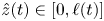 ${\hat {z}(t)\in [0,\ell (t)]}$ marks the interior of the fracture. Even for very small dimensionless viscosities (
 ${\mathcal {M}_{\hat {k}}\ll 1}$), the pressure gradient in the head from the 3-D numerical simulations is not entirely linear and presents a gentler slope than the limiting 3-D
  $\hat {K}$ GG (2014) solution (green dashed line; Garagash & Germanovich (Reference Garagash and Germanovich2014)). Only for the simulation with
  ${\mathcal {M}_{\hat {k}}=1\times 10^{-3}}$ is the viscous flow small enough to allow for a truly linear pressure gradient in the head. The shape of the opening is qualitatively similar between two and three dimensions (see
  ${\mathcal {M}_{\hat {k}}=1\times 10^{-3}}$), but the 2-D ones shrink in the direction of the buoyant force. The difference with the 2-D solution is directly related to 3-D effects associated with the curvature of the head.
The 3-D Garagash & Germanovich (Reference Garagash and Germanovich2014) and 2-D Roper & Lister (Reference Roper and Lister2007) solutions predict a negative net pressure at the end of the head. Our 3-D simulations do not show such a feature, and exhibit a smaller ‘neck’ than the one described by Roper & Lister (Reference Roper and Lister2007) in two dimensions. The ‘neck’ defines the region at the end of the head, where fracture opening is reduced compared to its stable value in the tail. This location is a pinch point leading to the influx of the fluid from the tail into the head. Nevertheless, figure 3 shows that the minimum pressure in the neck decreases with decreasing  ${\mathcal {M}_{\hat {k}}}$. We expect that a negative net pressure should appear for smaller values of
  ${\mathcal {M}_{\hat {k}}}$. These observations influence directly the opening distribution (figure 3a). We observe only a limited reduction of the opening between the tail and the head in the fully 3-D simulations. Nonetheless, such a neck is present, and an inflexion point can be identified (black circles in figure 3a). In the limit of zero fluid viscosity, the opening in the tail would become
  ${0}$. This would be when the neck fully pinches and a finite volume pulse forms.
4.4. Transient towards the late buoyant regime
In figure 2(c), an acceleration phase associated with the transition to buoyancy can be observed. Such an acceleration is related directly to the fact that when radial, the fracture velocity decreases with time as  $\ell _{k}\propto t^{2/5}$ and ultimately, once in the fully buoyant regime, reaches a constant velocity. The intensity of such acceleration can be related directly to the dimensionless number
  $\mathcal {M}_{\hat {k}}$ by comparing this terminal velocity with the radial velocity at the onset of buoyancy
  ${t=t_{k\hat {k}}}$ (see (3.6a,b)):
 \begin{equation} v_{\hat{k}}/v_{k}(t_{k\hat{k}})=\mathcal{M}_{\hat{k}}^{{-}1/3}.\end{equation}
The fracture needs to ‘catch up’ from a length  $\ell _{k}(t_{k\hat {k}})\sim \ell _{b}$ to the buoyant late-time solution (
 $\ell _{\hat {k}}(t_{k\hat {k}})\sim \mathcal {M}_{\hat {k}}^{-1/3}\ell _{b}$) and thus accelerates. According to figure 2(c), the acceleration starts approximately when
  ${t/t_{k\hat {k}}\approx 0.5}$. Correlating this with the observations of figure 2(a), this corresponds approximately to the time when the bulk of the head starts to leave the source region. The acceleration is thus driven by the pressure difference between the head and tail visible in figure 2(b). Figure 2(c) further shows that around
  ${t/t_{k\hat {k}}\approx 3}$, the fracture starts to decelerate and approaches the complete 3-D
  ${\hat {K}}$ solution (green dashed lines). The simulation then presents a good match until the end of the simulation (around
  ${t/t_{k\hat {k}}\approx 6.5}$). A convergence towards the linear, dominant term (green dash-dotted lines) is observed only once a simulation reaches about
  ${t/t_{k\hat {k}}\approx 10}$ (see the simulation with
  ${\mathcal {M}_{\hat {k}}=1\times 10^{-1}}$ in figure 2c). This is consistent with the approximate 3-D
  ${\hat {K}}$ GG (2014) solution, which predicts that linear velocity is reached within
  $5\,\%$ in relative terms when
  ${t/t_{k\hat {k}}\approx 14}$ (see the supplementary material available at https://doi.org/10.1017/jfm.2022.800 for details).
In the limiting case of zero fluid viscosity ( ${\mu ^{\prime }=0\to \mathcal {M}_{\hat {k}}=0}$), the acceleration is infinite, and we cannot hope to capture such a sharp transition numerically. The strictly
  $\mathcal {M}_{\hat {k}}=0$ limit corresponds to a 3-D Weertman pulse (Weertman Reference Weertman1971) associated with a zero-width tail. For very small but non-zero values of
  ${\mu ^{\prime }\,|\,\mathcal {M}_{\hat {k}}}$, overcoming the transition phase is numerically challenging but possible. Defining the end of the transient via the
  $5\,\%$ deviation level from the 3-D approximate solution (
 ${t/t_{k\hat {k}}\approx 14})$, we obtain a corresponding fracture length
  ${\ell (t)\sim 19\mathcal {M}_{\hat {k}}^{-1/3}\ell _{b}}$. Expressing this limit as the aspect ratio
  ${\ell (t)/b(t)}$, assuming that the breadth follows the Garagash & Germanovich (Reference Garagash and Germanovich2014) solution (
 ${b(t)\approx {\rm \pi}^{-1/3}\ell _{b}})$, the required aspect ratio is
  ${\ell (t)/b(t)\approx 28\mathcal {M}_{\hat {k}}^{-1/3}}$. The numerical example with
  ${\mathcal {M}_{\hat {k}}=1\times 10^{-2}}$ (largest value of
  ${\mathcal {M}_{\hat {k}}}$ validating the 3-D
  ${\hat {K}}$ solution) leads to a aspect ratio of
  ${\ell (t)/b(t)\sim 132}$ with a corresponding fracture length of
  ${\ell (t)\sim 90\ell _{b}}$. Such fracture lengths require a significant number of discretization cells. Numerically, the discretization is bounded mainly by two parameters: the distance of the source point to the fracture front, and the number of elements discretizing the head where a strong gradient of opening and pressure takes place. In the toughness-dominated case, the first parameter is more restrictive and requires discretizations of about
  ${44}$ elements per
  ${\ell _{b}}$. The total number of degrees of freedom thus quickly exceeds the current computational capacities of PyFrac (Zia & Lecampion Reference Zia and Lecampion2020) and ultimately explains why we do not report simulations for values of
  $\mathcal {M}_{\hat {k}}$ lower than
  $10^{-3}$.
5. Viscosity-dominated buoyant fractures ($\mathcal {M}_{\hat {k}}\gg 1$)

We now turn to the viscosity-dominated limit for which the transition to buoyancy occurs prior to the transition to the radial toughness-dominated regime:  $t_{m\hat {m}}\ll t_{mk}$, i.e.
  $\mathcal {M}_{\hat {k}}\gg 1$. We focus on the limiting case of a strictly zero-fracture toughness (
 ${\mathcal {M}_{\hat {k}}=\infty }$), which we will also refer to as the
  $\hat {M}$ limit (at late time). The evolution of such a fracture can be grasped from the numerical results reported in figures 4(e–i). Similar to the toughness case (figure 2), the fracture is initially radial (figure 4e) and elongates (figures 4 f–i) as soon as buoyancy plays a role (
 $t\sim t_{m\hat {m}}$). The overall footprint is strikingly different from the toughness limit. Notably, the fracture breadth is not uniform along the vertical direction and grows continuously horizontally due to the lack of any resistance to fracture. The shape of the fracture at late time is akin to an inverted cudgel with a distinct source and head regions.
Viscosity-dominated buoyant fracture. (a) Opening along the centreline  ${w(x=0,z,t)/w_{m\hat {m}}}$ for a simulation with
  ${\mathcal {M}_{\hat {k}}=\infty }$. (b) Net pressure along the centreline
  ${p(x=0,z,t)/p_{m\hat {m}}}$ for the same simulation. (c) Fracture length
  ${\ell (t)/\ell _{m\hat {m}}}$ for six simulations with large viscosity
  ${\mathcal {M}_{\hat {k}}\in [5\times 10^{2},\infty]}$. (d) Fracture breadth
  ${ b(t)/\ell _{m\hat {m}}}$ for the same simulations. (e–i) Evolution of the fracture footprint from radial (e) towards the final elongated inverse cudgel shape (h,i) for the same simulation as in (a) and (b).

5.1. Late-time zero-toughness limit
It is enlightening to compare this simulation for  $\mathcal {M}_{\hat {k}}=\infty$ with the scaling derived originally by Lister (Reference Lister1990b) for this problem (and his near-source solution). We first recall briefly the argument of such a scaling. Contrary to the toughness limit, the breadth is not constant, but the aspect ratio of the fracture remains related to the ratio of the characteristic horizontal
  $v_{x*}$ and vertical
  $v_{z*}$ fluid velocities:
 \begin{equation} \frac{b_{*}}{\ell_{*}}\sim\frac{v_{x*}}{v_{z*}}.\end{equation}
The horizontal and vertical extents are linked to their corresponding velocities as  $b_{*}=v_{x*}t$,
  $\ell _{*}=v_{z*}t$. Viscous fluid dissipation for viscous fractures occurs as much in the vertical as it does in the horizontal direction. Vertically, the net pressure gradient
  $\partial p/\partial z$ is negligible compared to
  ${\rm \Delta} \gamma$ such that, similarly to the viscosity-dominated tail in the
  $\hat {K}$ limit, the dimensionless ratio
 \begin{equation} \mathcal{G}_{mz}=\frac{\mu^{\prime}v_{z*}}{w_{*}^{2}\,{\rm \Delta}\gamma}\end{equation}
is of order 1. Horizontally, in the absence of gravitational forces, the magnitude of viscous flow is quantified by the ratio of the horizontal viscous pressure  ${\mu ^{\prime }v_{x*}b_{*}/w_{*}^{2}}$ to the characteristic net pressure
  ${p_{*}}$,
 \begin{equation} \mathcal{G}_{mx}=\frac{\mu^{\prime}v_{x*}b_{*}}{w_{*}^{2}p_{*}},\end{equation}
which is also of order one. Combined with elasticity ( $\mathcal {G}_{e}=1$) and global volume balance (
 $\mathcal {G}_{v}=1$), solving for the lengths, width and pressure scales, we recover the scaling of Lister (Reference Lister1990b):
 \begin{equation} \left.\begin{gathered} \ell_{\hat{m}}=\frac{{\rm \Delta}\gamma^{1/2}\,Q_{o}^{1/2}}{E^{\prime1/6} \mu^{\prime1/3}}\,t^{5/6},\quad b_{\hat{m}}=\frac{E^{\prime1/4}Q_{o}^{1/4}}{{\rm \Delta} \gamma^{1/4}}\,t^{1/4},\\ w_{\hat{m}}=\frac{Q_{o}^{1/4}\mu^{\prime1/3}}{{\rm \Delta}\gamma^{1/4}\, E^{\prime1/12}}\,t^{{-}1/12},\quad p_{\hat{m}}=\frac{E^{\prime^{2/3}}\mu^{\prime1/3}}{t^{1/3}}. \end{gathered}\right\} \end{equation}
Interestingly, in that scaling, the dimensionless toughness ( $\mathcal {G}_{k}\equiv \mathcal {K}_{\hat {m}}$) associated with horizontal growth (defined with
  $b_{*}$ as the characteristic fracture length) increases with time. From (2.13), we obtain the ‘horizontal’ (subscript
  $x$) dimensionless toughness
 \begin{equation} \mathcal{K}_{\hat{m},x}(t)=K_{Ic}\,\frac{{\rm \Delta}\gamma^{1/8}\,t^{5/24}}{E^{\prime19/24}Q_{o}^{1/8} \mu^{\prime1/3}}=\mathcal{M}_{\hat{k}}^{{-}3/14}\left(\frac{t}{t_{m\hat{m}}}\right)^{5/24}.\end{equation}
As a result, for the case of finite fracture toughness, one expects the horizontal growth to stop (and thus the breadth to stabilize) when  $\mathcal {K}_{\hat {m},x}(t)$ reaches order 1.
The time evolution of fracture length and breadth obtained numerically (figures 4c,d) exhibit a transition from the radial viscosity regime to this late buoyant viscous scaling. The power-law evolution with time of length and breadth matches (5.4) precisely at late time for the  $\mathcal {M}_{\hat {k}}=\infty$ simulation. Contrary to the toughness case, where the horizontal growth stops abruptly, we observe a smoother horizontal deceleration accompanied by vertical acceleration, which is less abrupt than in the toughness case.
In this zero-toughness limit, at late time, the growth of the fracture is self-similar and will not stop (either horizontally or vertically) as long as the volume release continues. To confirm the overall self-similarity of such a viscous, buoyant late-time regime, we rescaled our numerical results at different times and plot scaled footprints, centreline width and net pressure, as well as the volume of each horizontal cross-section in figure 5. The  ${z}$-axis is shifted such that the lowest point of the fracture coincides with
  ${\tilde {z}=0}$. A nice collapse of the scaled footprint is observed for
  ${t/t_{m\hat {m}}\gtrsim 100}$. A similar collapse appears for centreline sections of width, pressure and cross-section volume. We recognize that the head region shrinks with time and eventually reduces to a boundary layer. Before discussing the head region, we observe that the source region solution derived in Lister (Reference Lister1990b) matches our numerical results, albeit in a relatively narrow zone close to the injection point only. The Lister (Reference Lister1990b) solution is based on a pseudo-3-D approximation assuming only horizontal growth with an unspecified upper ‘head’ part. In this approximate solution, the breadth increases monotonically with the scaled coordinate
  $z/\ell _{\hat {m}}(t)$ without any possibility of reduction at large
  $z/\ell _{\hat {m}}(t)$ to model the fracture ‘head’. For the Lister (Reference Lister1990b) solution, the distance within which this source solution is applicable depends on the material, fluid and release properties. This distance is equivalent to the transition length scale of a fracture without buoyancy
  $\ell _{mk}$, which for the zero-toughness case becomes infinite. This solution, however, appears as the correct inner solution in the near-source region (but not up to
  $z\sim \ell _{mk}$). Further comparison of the width profiles at different cross-sections between our numerical solution and this approximation is reported in figure 6.
Scaled evolution of characteristic values of a buoyancy-driven viscosity-dominated fracture. Fracture footprint (a), cross-sectional volume, i.e. integral of the opening over the breadth (b), opening (c), and pressure (d) at various dimensionless times  ${t/t_{m\hat {m}}}$ . Blue dashed lines represent the pseudo-3-D near-source solution of Lister (Reference Lister1990b). A shifted coordinate system
  ${\tilde {z}}$ is used such that the lowest point of the fracture marks
  ${\tilde {z}=0}$.

Footprint and cross-sectional opening profiles of two buoyant, viscosity-dominated fractures. The colour code of the fractures represents the scaled opening as described at the top. Black lines correspond to opening-profile evaluations. The horizontal blue dashed line in (a) is the limiting height for the viscous solution of Lister (Reference Lister1990b). Blue dashed lines in (a,e) show the Lister (Reference Lister1990b) solution. Red dashed lines mark the maximum breadth and the beginning of the head. (b–d) Opening profiles in the cross-section, where blue dashed lines represent the Lister (Reference Lister1990b) solution, dash-dotted lines correspond to  ${\mathcal {M}_{\hat {k}}=\infty }$, and continuous lines correspond to
  ${\mathcal {M}_{\hat {k}}=10^{5}}$.

5.1.1. Head region
From both the footprints with width contours displayed in figure 4 and the scaled profiles in figure 5, we observe that, contrary to the toughness case, the head region shrinks with time. Self-similarity of the overall fracture growth actually becomes evident when the volumes of the head and the source region are negligible compared to the volume in the tail, i.e. for times greater than  ${\sim }100 t_{m\hat {m}}$. The depletion of the head can be explored by the following scaling argument. In a viscous head (
 $b_{*}^{{head}}\sim \ell _{*}^{{head}}$), the horizontal and vertical fluid velocities are of the same order, elasticity (
 $\mathcal {G}_{e}=1$) and buoyancy (
 $\mathcal {G}_{b}=1$), and viscous dissipation dominates (
 $\mathcal {G}_{mz}=1$), but its volume is a priori unknown. In addition, we assume that the characteristic fluid velocity in the head is given by the vertical characteristic velocity
  ${v_{z\hat {m}}}\sim {\ell _{\hat {m}}/t}$ from (5.4). In other words, the volumetric flow rate between the head and the tail is
  ${Q_{*}=w_{*}^{{head}}b_{*}^{{head}}v_{z\hat {m}}}$. Under those assumptions, the corresponding characteristic viscous head scales are
 \begin{equation} \left.\begin{gathered} \ell_{\hat{m}}^{{head}}=b_{\hat{m}}^{{head}}= \frac{E^{\prime11/24}Q_{o}^{1/8}\mu^{\prime1/6}}{{\rm \Delta}\gamma^{5/8}\,t^{1/24}},\quad w_{\hat{m}}^{{head}}=\frac{Q_{o}^{1/4}\mu^{\prime1/3}}{E^{\prime1/12}\,{\rm \Delta}\gamma^{1/4}\,t^{1/12}}, \\ p_{\hat{m}}^{{head}}=\frac{E^{\prime11/24}Q_{o}^{1/8}\mu^{\prime1/6}\,{\rm \Delta}\gamma^{3/8}}{t^{1/24}},\quad V_{\hat{m}}^{{head}}=\frac{E^{\prime5/6}Q_{o}^{1/2}\mu^{\prime2/3}}{{\rm \Delta}\gamma^{3/2}\,t^{1/6}}. \end{gathered}\right\} \end{equation}
These characteristic scales are consistent with the shrinking/depleting viscous head observed numerically. The numerical validation is presented in table 2, where we observe the evolution of the head length, the head volume, and the maximum opening in the head. Even thoughwe do not have an analytical or semi-analytical solution to compare to, stabilization, when normalized with the depleting scales (5.6), is observed in table 2 within the precision of our automatic evaluation of the head length. It is interesting to note that at the onset of buoyancy, for  ${t\approx t_{m\hat {m}}}$ (defined in (3.6a,b)), these scales are strictly equal to the radial viscosity-dominated scales (e.g.
  $\ell _{\hat {m}}^{{head}}(t_{m\hat {m}})=\ell _{m}(t_{m\hat {m}})$,
  $V_{\hat {m}}^{{head}}(t_{m\hat {m}})=Q_{o}t_{m\hat {m}}$). This confirms the mechanism of a viscous head that detaches from the source region and slowly depletes as it moves upward.
Comparison between characteristic head length, head volume and maximum opening in the head ( ${w_{{max}}^{{head}}=\max _{x,z} \{w(x,z\in [z_{tip}-\ell ^{{head}}(t),z_{tip}],t)\} }$) for viscosity-dominated fractures
  ${ \mathcal {M}_{\hat {k}}\in [1\times 10^{4},\infty]}$ at various dimensionless times
  ${t/t_{m\hat {m}}}$.

5.1.2 Comparison with the semi-infinite plane-strain solution
Such a 3-D viscous head can be compared to the existing 2-D plane-strain solution for a viscosity-dominated steadily moving buoyant fracture (Lister Reference Lister1990a). The 2-D scales of Lister (Reference Lister1990a) are based on a constant fracture velocity. For the 3-D case, the characteristic fracture velocity  $v_{z\hat {m}}$ decreases as
 \begin{equation} v_{z\hat{m}}=\frac{\ell_{\hat{m}}}{t}=\frac{{\rm \Delta}\gamma^{1/2}\, Q_{o}^{1/2}}{E^{\prime1/6}\mu^{\prime1/3}t^{1/6}}, \end{equation}
which can be translated into a reducing 2-D release rate by multiplication with the characteristic tail opening
 \begin{equation} Q_{2D}\sim v_{z\hat{m}}w_{\hat{m}}\sim\frac{Q_{o}^{3/4}\, {\rm \Delta}\gamma^{1/4}}{E^{\prime1/4}t^{1/4}}.\end{equation}
Replacing this injection rate into the scales of Lister (Reference Lister1990a), we retrieve exactly the scaling of (5.6). Rescaled 3-D numerical results are shown along with the zero-toughness solution of Lister (Reference Lister1990a) using a tip-based coordinate system ( ${\hat {z}(t)=z_{tip}(t)-z}$) in figure 7. The 3-D and 2-D solutions practically coincide (relative error
  $\sim 5\,\%$) for times
  ${t\gtrsim 50t_{m\hat {m}}}$. In the viscosity-dominated case, the shrinking of the head indeed reduces the effect of the 3-D curvature at large time (see also the scaled footprint in figure 5) and thus renders the elastic state of plane-strain more valid.
Tip-based opening (a) and pressure (b) of a viscosity-dominated buoyant simulation with  ${\mathcal {M}_{\hat {k}}=\infty }$ as a function of the scaled tip coordinate. Continuous lines correspond to the simulations with PyFrac (Zia & Lecampion Reference Zia and Lecampion2020), with dots marking the locations of discrete evaluations. The dash-dotted line shows the 2-D plane-strain steadily moving solution (see details in the supplementary material available at https://doi.org/10.1017/jfm.2022.800).

In conclusion, the buoyant viscosity-dominated fracture exhibits a viscous source region following the Lister (Reference Lister1990b) solution, combined with a depleting head according to the scaling (5.6) at the propagating edge for late times ( $t\gg t_{m\hat {m}}$). The depleting head follows the solution of a 2-D semi-infinite plane-strain fracture along the centreline. It may be possible to construct a complete pseudo-3-D approximation matching these asymptotes in the source and head region, a task we leave open for further studies.
6. Intermediate/finite $\mathcal {M}_{\hat {k}}$ cases

In the toughness-dominated case, we have seen that the  $\hat {K}$ limit is captured by the Garagash & Germanovich (Reference Garagash and Germanovich2014) finger-like solution for
  ${\mathcal {M}_{\hat {k}}\lesssim 1\times 10^{-2}}$. On the other end, for zero-toughness (
 ${\mathcal {M}_{\hat {k}}=\infty }$), horizontal growth continues as
  $\sim t^{1/4}$ at late times (
 $t\gtrsim 100t_{m\hat {m}}$). Numerical results for large but finite values of
  $\mathcal {M}_{\hat {k}}$ (see figures 4c,d) show that, as anticipated (Lister Reference Lister1990b; Garagash & Germanovich Reference Garagash and Germanovich2022), horizontal growth arrests after some time. The vertical velocity thus increases to a constant terminal velocity due to volume balance. This is confirmed by the
  $\mathcal {M}_{\hat {k}}=500,10^{3}$ simulations displayed in figures 4(c,d) (and to a lesser extent for
  $\mathcal {M}_{\hat {k}}=10^{4}$ where the horizontal arrest was not reached completely). The characteristic time scale for such a horizontal arrest can be estimated as the time at which the horizontal dimensionless toughness
  $\mathcal {K}_{\hat {m},x}$ of (5.5) in the viscous tail scaling reaches order 1. We obtain
 \begin{equation} \mathcal{K}_{\hat{m},x}\left(t_{\hat{m}\hat{k}}^{x}\right)=1\rightarrow t_{\hat{m}\hat{k}}^{x}=\frac{E^{\prime19/5}Q_{o}^{3/5}\mu^{\prime8/5}}{K_{Ic}^{24/5}\, {\rm \Delta}\gamma^{3/5}}=\mathcal{M}_{\hat{k}}^{36/35}t_{m\hat{m}},\end{equation}
and the corresponding maximum breadth and length scales are
 \begin{equation} b_{\hat{m}}\left(t_{\hat{m}\hat{k}}^{x}\right)= \mathcal{M}_{\hat{k}}^{2/5}\ell_{b},\quad \ell_{\hat{m}} \left(t_{\hat{m}\hat{k}}^{x}\right)=\ell_{mk}.\end{equation}
From our previous discussion, the zero-toughness ( ${\mathcal {M}_{\hat {k}}=\infty }$) self-similar growth is established for
  $t\gtrsim 100t_{m\hat {m}}$. For large values of
  $\mathcal {M}_{\hat {k}}$, such a zero-toughness solution is thus expected to be realized at intermediate times after the transition to buoyancy but prior to the characteristic time of horizontal arrest, i.e. for
  $t\in [100 t_{m\hat {m}},t_{\hat {m}\hat {k}}^{x}]$. Using (6.1), we thus expect to see a period of lateral growth for dimensionless viscosities at least larger than
  $\mathcal {M}_{\hat {k}}^{36/35}\sim \mathcal {M}_{\hat {k}}=100$.
We performed a series of simulations spanning a wide range of values of  $\mathcal {M}_{\hat {k}}$ from
  $10^{-3}$ to
  $10^{3}$ for which the simulations were run long enough to observe a cessation of horizontal growth. We report in figure 8 the evolution of the maximum breadth of the buoyant fracture with
  $\mathcal {M}_{\hat {k}}$. As expected, in the toughness-dominated limit
  $\mathcal {M}_{\hat {k}}<1$, the fracture breadth remains close to the
  $\hat {K}$ limit. The maximum breadth then increases with
  $\mathcal {M}_{\hat {k}}$, from the Garagash & Germanovich (Reference Garagash and Germanovich2014)
  $b\sim {\rm \pi}^{-1/3}\ell _{b}$ solution for
  $\mathcal {M}_{\hat {k}}<10^{-2}$, up to
  $b\sim 5\ell _{b}$ for
  $\mathcal {M}_{\hat {k}}=100$. For values up to
  $\mathcal {M}_{\hat {k}}\sim 100$, we always observe a uniform breadth along the fracture footprint, and no horizontal growth is observed after the transition to buoyancy. These fractures have a clear finger-like shape. It is worth noting that from their approximate 3-D toughness solution, Garagash & Germanovich (Reference Garagash and Germanovich2014) obtain a lower value (
 ${\mathcal {M}_{\hat {k}}\approx 0.92}$) as a criterion for no further horizontal growth. Accounting for fully 3-D effects, the domain of ‘finger-like’ fracture shapes is seen to extend up to
  $\mathcal {M}_{\hat {k}}=100$.
Comparison of maximum breadth for buoyant fractures as a function of the dimensionless viscosity  ${\mathcal {M}_{\hat {k}}\in [10^{-3},5\times 10^{3}]}$. Black dots are used for fractures with a uniform breadth, and red stars are used otherwise. The dashed green lines represent the limits of the 3-D
  ${\hat {K}}$ GG (2014) solution (
 ${b\sim {\rm \pi}^{-1/3}\ell _{b}}$ for the breadth limit (horizontal line) and
  ${\mathcal {M}_{\hat {k}}\approx 0.92}$ for the stabilization criterion (vertical line)). The grey dashed line emphasizes the scaling relation
  $\max _{z,t}\{ b(z,t)\} \sim \mathcal {M}_{\hat {k}}^{2/5}\ell _{b}$.

For values  $\mathcal {M}_{\hat {k}}>100$, the fractures have a distinctly different late-time shape akin to an inverted cudgel (non-uniform horizontal breadth) with an ultimately fixed maximum horizontal breadth. We recover the predicted evolution of the maximum breadth (6.2a,b) as
  ${\mathcal {M}_{\hat {k}}^{2/5}\ell _{b}}$ (red stars in figure 8). A fit of our numerical results actually provides
  $\max _{z,t}\{ b(z,t)\} \approx 0.6858\mathcal {M}_{\hat {k}}^{2/5}\ell _{b}$ for
  ${\mathcal {M}_{\hat {k}}\in [10^{2},2\times 10^{3}]}$. Using this fitted pre-factor on the breadth evolution, assuming
  $b\sim b_{\hat {m}}(t)$ before stabilization, we estimate the time for breadth stabilization to be
  ${{\sim }0.22t_{\hat {m}\hat {k}}^{x}}$. We show graphically in figure 9 that this estimation agrees fairly well with the numerical results. For the reported simulations, the fracture length ultimately evolves linearly in time (indicated by a 1 : 1 slope in figure 9) as
  ${\ell (t)/\ell _{m\hat {m}}\sim \mathcal {M}_{\hat {k}}^{-6/35}(t/t_{m\hat {m}})}$.
Evolution of fracture breadth and length for intermediate fractures without a uniform breadth  ${\mathcal {M}_{\hat {k}}\in [10^{2},2\times 10^{3}]}$ (the simulation with
  ${\mathcal {M}_{\hat {k}}=\infty }$ is used as a reference). Dashed lines show fracture breadth, continuous lines fracture height, and horizontal dash-dotted lines the expected time where lateral growth stops. The emerging power laws are indicated.

We also performed simulations for  $\mathcal {M}_{\hat {k}}>10^{3}$, which, however, did not reach the arrest of horizontal growth within a reasonable computational time limit. It is worth pointing out that from these numerical results, the self-similar viscous (
 ${\mathcal {M}_{\hat {k}}=\infty }$) evolution is actually visible at intermediate times only for dimensionless viscosities larger than
  $10^{4}$ (see figures 4c,d).
7. Discussion
7.1. Orders of magnitude
In nature, buoyant HFs are suggested to be a major contributor to the transport of magma through the lithosphere (Rivalta et al. Reference Rivalta, Taisne, Bunger and Katz2015). For such cases, data collection is difficult and often restricted to the investigation of outcrops from dykes. A broad range of rarely well-constrained parameters is possible. We thus only briefly illustrate the emergence of dykes using the following parameters (Möri & Lecampion Reference Möri and Lecampion2021):  $E^{\prime }\sim 10\,\textrm {GPa}$,
  $K_{Ic}\sim 1.5\,\textrm {MPa}\,\textrm {m}^{1/2}$,
  $\mu _{f}=100\,\textrm {Pa}\,\textrm {s}$,
  ${\rm \Delta} \rho \sim 250\,\textrm {kg}\,\textrm {m}^{-3}$, and a low value of the release rate
  $Q_{o}\sim 1\,\textrm {m}^{3}\,\textrm {s}^{-1}$. For this set of parameters, the dyke intrusion is strongly viscosity-dominated with
  ${\mathcal {M}_{\hat {k}}\approx 3.29\times 10^{6}}$, and has a maximum lateral extent of tens of kilometres. The use of a higher release rate would linearly increase the value of
  ${\mathcal {M}_{\hat {k}}}$ and thus only render the growth more viscosity-dominated. The corresponding fracture height easily exceeds the thickness of the lithosphere, as already pointed out by Lister (Reference Lister1990b). As a result, such large extents will necessarily clash with the length scales of stress and material heterogeneities. It also indicates the very strong effect of buoyancy on upward growth.
7.2. Comparison with experiments
Various experiments on buoyant fractures have been performed in the laboratory (Heimpel & Olson Reference Heimpel and Olson1994; Ito & Martel Reference Ito and Martel2002; Rivalta, Böttinger & Dahm Reference Rivalta, Böttinger and Dahm2005; Taisne & Tait Reference Taisne and Tait2009; Taisne, Tait & Jaupart Reference Taisne, Tait and Jaupart2011). Most of these experiments consist of a finite (not continuous) release, and aim at investigating various mechanisms (arrest due to material heterogeneities among other things). In figure 10(a), we evaluate the evolution of the fracture velocity with time for the experiments performed by Heimpel & Olson (Reference Heimpel and Olson1994). The data in their figure 2 are transformed to correspond to our scaled velocity and time. All experimental parameters except the release rate  $Q_o$ are taken from Heimpel & Olson (Reference Heimpel and Olson1994). The good match of figure 10(a) was obtained using an estimate of the release rate
  $Q_{o}\sim 10^{-8}\,\textrm {m}^{3}\,\textrm {s}^{-1}$. The corresponding dimensionless viscosities are in the range
  ${\mathcal {M}_{\hat {k}}\in [8.8\times 10^{-8},2.3\times 10^{-3}]}$ (see details in the supplementary material available at https://doi.org/10.1017/jfm.2022.800). When superimposing their velocity evolution onto our numerical results for
  ${\mathcal {M}_{\hat {k}}\in [10^{-3},10^{-1}]}$, we observe that their experiments start in the transition between the radial and buoyant regimes. In other words, their experiments are situated within the accelerating phase, and their velocities tend to stabilize only towards the very end of the experiment. Some experiments show a deceleration but do not quite reach a constant velocity as the time to overcome the transient (
 ${t/t_{k\hat {k}}\approx 14}$) is reached in none of the experiments. This is a direct consequence of the limited sample size, which is insufficient in all experiments to reach the end of the transient regime (see details in the supplementary material available at https://doi.org/10.1017/jfm.2022.800). We thus conclude that these experiments are strongly influenced by their initial conditions (a too-large initial notch) and the finiteness of the specimens, which prevents them from reaching the constant terminal velocity.
(a) Comparison of the experiments of Heimpel & Olson (Reference Heimpel and Olson1994) with our simulations. The experiment takes place within the transient, and the initiation already favours the buoyant propagation. (b) Comparison of estimated and observed breadth for two experimental studies.

As described in § 4.2, in that range of such low dimensionless viscosities, we can nevertheless compare the fracture breadth in the transient phase. We could extract information on the fracture breadth from two contributions, albeit with uncertainties on some reported parameters. We assume that for such toughness-dominated buoyant fractures, the  $\hat {K}$ solution of Garagash & Germanovich (Reference Garagash and Germanovich2022) is also valid in the case of a finite volume release, which allows us to use the data from Taisne & Tait (Reference Taisne and Tait2009). In figure 10(b), we report the measured breadth
  ${b^{{exp}}}$ and compare it to the limiting 3-D
  $\hat {K}$ GG (2014) solution
  ${{\rm \pi} ^{-1/3}\ell _{b}}$. The breadth is generally underestimated for both contributions. In most cases, the extension of the fracture in these experiments clashes with the finite size of the sample, and the initial notch size might be inadequate. These boundary and initiation effects may also modify the linear gradient of the background stress and thus render the evaluation of
  ${{\rm \Delta} \gamma }$ erroneous.
7.3. Possibility of approximate solutions
The computational cost of the reported simulations is considerable and tests the limits of the numerical solver used herein (see § 2.2 for details). For example, the simulations presented in figures 2 and 4 took between two and two and a half weeks on a multithreaded Linux desktop system with twelve Intel![]() Core i7-8700 CPUs, and used at most 30 GB of RAM. Such requirements are common for the simulations presented in this paper.
Core i7-8700 CPUs, and used at most 30 GB of RAM. Such requirements are common for the simulations presented in this paper.
Interestingly, our results point to the possible development of reduced-order pseudo-3-D models (Adachi & Peirce Reference Adachi and Peirce2008; Adachi, Detournay & Peirce Reference Adachi, Detournay and Peirce2010) that would inevitably be much more efficient computationally. For example, the 3-D  $\hat {K}$ GG (2014) solution of Garagash & Germanovich (Reference Garagash and Germanovich2022) is based on a finger-like fracture approximation for the tail while keeping a complete description of the elasticity in the head region. We could demonstrate the validity of this assumption as discussed in § 4. Employing the knowledge gained from our results, the development of accurate and computationally efficient models similar to the ones presented in Dontsov & Peirce (Reference Dontsov and Peirce2015) may be possible. The solution derived in Lister (Reference Lister1990b) is based on a similar approach for the zero-toughness case. We could show that this approach works fairly well within the source region but fails to capture the transition to the head region, which has not been prescribed in the work of Lister (Reference Lister1990b). The insights gained from our simulations (see § 5.1) could be used to develop further an enhanced pseudo-3-D model for the viscous case. Such a model could then possibly bridge the source region solution of Lister (Reference Lister1990b) with a viscous head.
8. Conclusions
For a homogeneous linear elastic solid subjected to a linear background confining stress and a Newtonian fluid, using numerical simulations and scaling analysis, we have shown that under a constant release rate, the growth of 3-D buoyant fractures is governed by a single dimensionless number  $\mathcal {M}_{\hat {k}}$ (see (3.9)). It is worth emphasizing the very large computational cost of the simulations reported here, which span more than ten, respectively twenty, orders of magnitude in space and time. They reach the computational limit of our current implementation of the ILSA. Nonetheless, from this series of simulations, we have shown that a family of buoyant hydraulic fractures (HFs) emerges at late times as a function of
  $\mathcal {M}_{\hat {k}}$. The solution phase space can be summarized in the diagram displayed in figure 11. At early time, all fractures start with a radial shape and are initially dominated by viscous dissipation (
 $ {M}$), and remain radial for times lower than the buoyancy transition time scales (3.6a,b). Depending on the ratio between the radial viscosity to toughness transition time scale
  $t_{mk}$ (without buoyancy) and the viscous buoyancy transition time scale
  $t_{m\hat {m}}$ (or
  $t_{k\hat {k}}$), encapsulated in the definition of the dimensionless viscosity
  $\mathcal {M}_{\hat {k}}$ in (3.9), a family of solutions exists at late time when buoyancy dominates. If the transition to buoyancy occurs when the HF is already in the toughness-dominated regime (
 ${\mathcal {M}_{\hat {k}}\lesssim 10^{-2}}$), then the late time growth is well captured by the
  ${\hat {K}}$ approximate solution of Garagash & Germanovich (Reference Garagash and Germanovich2014). In this limit of large toughness, the buoyant HF has a distinct toughness-dominated head with a constant volume and shape, and a viscosity-dominated tail that governs its upward growth. For an intermediate range
  ${\mathcal {M}_{\hat {k}}\in [10^{-2},10^{2}]}$, the fracture remains finger-like with a uniform breadth for each cross-section, albeit with an increasing breadth with
  $\mathcal {M}_{\hat {k}}$. Above
  $\mathcal {M}_{\hat {k}}>100$, the HFs exhibit an inverted cudgel shape at late time (the breadth is no longer spatially uniform in the tail), and the maximum horizontal breadth increases as
  $\mathcal {M}_{\hat {k}}^{2/5}\ell _{b}$ as horizontal growth occurs until a given time
  $t_{\hat {m}\hat {k}}^{x}$ (see (6.1)). For values
  ${\mathcal {M}_{\hat {k}}\gtrsim 10^{4}}$, a zero-toughness self-similar
  $\hat {M}$ limit (§ 5) can be observed at intermediate times. This self-similar
  $\hat {M}$ viscosity-dominated limit exhibits an ever-increasing breadth in association with thezero-toughness assumption. The scaling of the
  $\hat {M}$, regime originally presented in Lister (Reference Lister1990b), is confirmed by our numerical results. In that limit, the viscous head is slowly depleting with time with a centreline evolution akin to the known 2-D plane-strain near-tip asymptotic solution at late time. It might be possible to develop an approximate solution for that viscous limit along similar lines as in the toughness-dominated case when combining the source solution and the near-tip viscous head. A finite toughness always ensures an ultimate arrest of horizontal growth at a characteristic time
  $t_{\hat {m}\hat {k}}^{x}=\mathcal {M}_{\hat {k}}^{36/35}t_{m\hat {m}}$ for which the horizontal dimensionless toughness becomes of order 1. Besides their final shapes, another important difference between buoyant toughness-dominated HFs and viscous ones lies in the transition to the buoyant regime. For toughness-dominated fractures, a significant vertical acceleration (
 $\propto \mathcal {M}_{\hat {k}}^{-1/3}$) is observed, whereas viscosity-dominated fractures have a smoother vertical acceleration thanks to horizontal growth.
Propagation diagram for 3-D buoyant fractures under a continuous fluid release. Radial growth is initially viscosity-dominated ( ${M}$). Transition to buoyancy occurs either before (
 ${\mathcal {M}_{\hat {k}}}\gg 1$) or after (
 ${\mathcal {M}_{\hat {k}}}\ll 1$) the transition to radial toughness-dominated growth. At late times, a family of buoyancy-driven solutions as a function of
  ${\mathcal {M}_{\hat {k}}}$ (see (3.9)) emerges. The large toughness limit (§ 4) is reached for values
  ${\mathcal {M}_{\hat {k}}\lesssim 10^{-2}}$, whereas the zero-toughness solution (§ 5) appears at intermediate times
  $t\in [100t_{m\hat {m}},t_{\hat {m}\hat {k}}^{x}]$ for
  ${\mathcal {M}_{\hat {k}}\gtrsim 10^{4}}$.

Natural magmatic buoyant fractures are likely always viscosity-dominated, while on the other hand, all laboratory experiments have been performed under toughness-dominated conditions. It appears that even in the toughness regime, precise experiments are still lacking quantitative comparison with the theoretical predictions reported here for buoyant fractures. Orders of magnitude for magmatic dykes also indicate that their horizontal and vertical extents will necessarily clash with length scales of stress and material heterogeneities at late times. These heterogeneities, as well as the possibility of fluid exchange with the surrounding rock and thermal effects, may play a critical role in the growth and potential arrest of buoyant HFs on their way towards the surface. The interplay of these effects on linear HF mechanics growth remains to be investigated. Finally, most fluid releases are of a finite volume rather than having an ever-ongoing release at a constant injection rate. This particular problem is part of ongoing research and is essentially based on the findings presented in this paper.
Supplementary material
Supplementary material is available at https://doi.org/10.1017/jfm.2022.800.
Acknowledgements
The authors gratefully acknowledge in-depth discussions with D. Garagash regarding the 3-D toughness-dominated approximate solution presented in Garagash & Germanovich (Reference Garagash and Germanovich2014, Reference Garagash and Germanovich2022) and Germanovich et al. (Reference Germanovich, Garagash, Murdoch and Robinowitz2014).
Funding
This work was funded by the Swiss National Science Foundation under grant no. 92237.
Declaration of interests
The authors report no conflict of interest.
Data availability statement
The version of the open-source solver PyFrac, corresponding scripts and results of simulations in this study are openly available at 10.5281/zenodo.6511166.
Author contributions
A.M. contributed to conceptualization, methodology, formal analysis, investigation, software, validation, visualization, writing original draft. B.L. contributed to conceptualization, methodology, formal analysis, validation, supervision, funding acquisition, writing review and editing.
Appendix. Recapitulating tables of scales
For completeness, we list all the scales used within this paper in tables 3 and 4. A Wolfram Mathematica notebook containing their derivation and the different scalings is further provided in the supplementary material available at https://doi.org/10.1017/jfm.2022.800.
Characteristic scales (and governing dimensionless parameters  $\mathcal {P}_{s}$) in the different scalings.

Transition scales between regimes. The toughness head scales in table 3 correspond to the transition scales  ${K}\rightarrow \hat {K}$.


 Open access