

Introduction
The main purpose of palaeoclimate modelling is to produce experiments which study the basic interactions of the different parts of the climate system (atmosphere, hydrosphere, cryosphere, lithosphere and biosphere) and their long-term variability.
Many models designed to address the ice-age cycle use an annual net mass-balance function which depends on the snow-line parameterization; or degree-day factor, which is generally calibrated using present-day measurements. Such parameterizations over-simplify a great number of complex processes and take insufficient account of the seasonal cycle and latitudinal distribution of insolation. The sensitivity is arbitrarily fixed and the model conception restricts the number of processes that can be responsible for amplification of the solar forcing. Seasonal models thus seem to be absolutely necessary. For the present, however, atmospheric general-circulation models (CCMs) seem to be unable to yield a reliable quantitative computation of the net snow accumulation (Reference OglesbyOglesby, 1990), while coupling with oceanic CCMs and other complex climatic sub-system models (sea-ice, biosphere) is unrealizable For long simulations, Simple coupled climate/cryosphere models, on the other hand, allow us to study a great number of physical processes such as those related to snow and ice accumulation and ablation. Low computer cost allows us to integrate these models over a long time period and run a great number of sensitivity experiments.
1. The Models
We have coupled a fine-grid horizontal (latitude, longitude) model (CIM, continental surface and ice-sheet model) able to represent the inception, waxing and waning of the ice sheets on the Earth’s surface, to the two-dimensional LLN (Louvain-la-Neuve) climate model (latitude, altitude) representing in zonal mean the different parts of the climate system for the Northern Hemisphere (atmosphere, ocean, sea ice, continental surface covered or not by snow) (Reference Gallée, van Ypersele, Fichefet, Tricot and Berger.Gallée and others. 1991, Reference Gallée, van Ypersele, Fichefet, Marsiat, Tricot and Berger.1992).
The LLN climate model is latitude-, surface- and altitude-dependent. Its domain covers the Northern Hemisphere with a resolution of 5° latitude. Atmospheric dynamics are represented by a zonally averaged quasi-geostrophic model, including parameterization of the meridional transport of quasi-geostrophic potential vorticity and of the Hadley sensible-heat transport. The atmosphere interacts with the other components of the climate system through vertical fluxes of momentum, heat and water vapour. The model explicitly incorporates detailed radiative-transfer schemes, surface-energy balances, and snow and sea-ice budgets. The vertical profile of the upper-ocean temperature is computed by an integral mixed-layer model which takes into account the meridional convergence of heat. Sea ice is represented by a thermodynamic model including leads and lateral accretion.
The CIM horizontal model we developed combines three parts; a model representing ice dynamics; a model representing- the depression of the asthenosphere under the weight of the ice; and the mass-balance evaluation over the ice sheets and over the continents.
The ice-sheet model
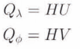
The ice-sheet model is a vertically integrated ice-dynamics model, written in spherical coordinates, which can be integrated all over the Earth. To avoid the singularity of the poles, we substitute for the horizontal velocities (v, v) the new fields U and V defined as:

whore ϕ is the latitude and r is the radius of the Earth. The mass fluxes are:
where λ is the longitude, and at the poles (ϕ = ±) U = V = 0 and Qλ = Qϕ = 0.
The full set of equations governing the ice motion is then


where H = h − b is the ice thickness, b is the bedrock elevation with respect to sea level, h is the ice-surface elevation with respect to sea level, μ = sin ϕ, M is the mass balance over the ice-sheet surface and ρ is the density of ice which is assumed to be homogeneous. The factor A relating strain rate and deviator tensor in the generalized flow law depends mainly on the temperature. In the present model, the temperature distribution in the ice is not computed and a constant value of A is used. On the other hand, we do not make a distinction between internal deformation and basal sliding, so A can be adjusted to allow crudely for basal sliding.
This highly non-linear set of equations is solved on a spherical grid composed of 257 circles in latitude, each including 256 equidistant points in longitude. This represents a grid mesh of 1.4° longitude to 0.7° latitude, corresponding to a 27.2 km × 77.8 km grid mesh at 80° N.
A thin-channel model is used on a spherical grid to compute the sinking of the crust under the weight of the ice. Sea-level variations associated with variations in ice volume are calculated. The model does not take into account the possible existence of ice shelves; calving of ice occurs when ice floats.
The mass-balance model
One of the most important parts of an ice-sheet model is the computation of the annual net mass balance. In the present model, the annual cycle of surface temperature and the seasonal evolution of a possible snow layer are computed at each continental point (whether covered with snow or not). A complete description of the model is given by Reference Marsiat.Marsiat (in press).
In regions where some precipitation falls as snow, one can observe the following situations:
The summer temperature remains sufficiently high to melt the snow accumulated during winter. The snowfield is non-permanent.
The snow survives during summer. The minimum thickness of snow observed during summer remains constant from year to year. The snowfield is permanent and stable with zero mass balance.
The minimum thickness of snow grows from year to year. A thickening snowfield or névé forms at this point, which, if maintained for a sufficiently long time, will compact to form a glacier or an ice sheet. The mass balance M is computed from the inter-annual variation of the minimal snow thickness h s:
At the ice-sheet surface, the net mass balance is computed from the difference during an annual cycle between snow precipitation and snow melting. When the snow accumulated in winter is completely melted, the summer heating melts the underlying ice.
The annual cycle of surface temperature is computed from balance between atmospheric fluxes reaching the surface, seasonal heat transfer and storage in the soil, and heat conduction in the snow layer where it exists. When the computed temperature of the snow or ice surface exceeds the freezing temperature T f = 273.15 K, the surface temperature is reset to T f and the excess of energy LM is used to melt the snow or ice. The thickness of snow Δh s melted during a time step Δt is then:

where ρ s = 330 kg m−3 is the density of snow and L f = 0.33 × 10⁶ J kg−1 is the latent heat of fusion.
As solar radiation often represents the main energy source for modification of the snow cover, knowledge of interactions between the radiation and the snow is fundamental for the energy and mass balance of the snow mantle. The snow albedo is not constant in time and may vary considerably, e.g. under the influence of the snow-aging process. Simulations conducted by Galléc and others (1992) show the importance of the snow-albedo modification in the degradation processes. We distinguish two types of vegetation rover: low-vegetation cover, such as steppes or tundra, and the high-vegetation, forest type, or taiga. Because snow rarely covers the treetops. the albedo of the forest covered by snow, α s = 0.4, is much lower than the albedo of the snow-covered fields. Over tundras and ice sheets, the snow-surface albedo is a function of snow-precipitation frequency and snow-surface temperature. Albedo values range from 0.85 for cold fresh snow to 0.4 for old melting snow. On the other hand, when the snow thickness is < 10 cm, the albedo decreases linearly in the albedo of the underlying surface. To prevent any intense cooling of the mountain areas, it is also assumed that the snow does not cover the entire grid mesh of the high-altitude regions (z ≤ 1500 m) until the thickness of the snow reaches 5 m.
Because not much is known regarding past precipitation rates and precipitation fields are unreliably predicted by present-day GCMs, we compute for each grid point a local annual cycle of precipitation, calibrated using the present data but strongly dependent on the local slope and on the local temperature variations in time. The fraction of precipitation falling as snow is a function of the local temperature. Details of the precipitation parameterization are given by Reference Marsiat.Marsiat (in press).
The coupling
The coupling between the CIM and LLN models is achieved by the use in the CIM model of the following zonally averaged quantities computed by the LLN model:
the solar and long-wave downward fluxes;
a term representing the contribution of the diurnal and synoptic temperature variance to the sensible-heat flux;
the 500 mbar level temperature;
the zonal annual mean precipitation rate.
Inversely, the CIM provides the LLX model with the spatial extent and the mean altitude of the ice sheets.
The coupling between a horizontal model of continental surfaces (latitude–longitude) like the CIM model and a zonally averaged vertical climate model (latitude altitude) like the LLN model is not easy to realize. It is assumed that at the 500 mbar level, for all points situated at the same latitude, the atmosphere is identical to the zonal mean computed by the LLN model. Local radiative fluxes and temperature at the top of the boundary layer are then interpolated from the zonal means, taking into account local characteristics such as altitude. Details of the interpolation process are given by Reference Marsiat.Marsiat (m press).
The coupling of the models is asynchronous, with an equilibrium climatic state of the LLN model computed every 1000 years. In the CIM model, we do not restrain the growth domain of the ice sheets, in contrast to the experiments conducted by Reference Deblonde and PeltierDeblonde and Peltier (1991). Their ice-sheet model is solved only within pre-defined sub-domains corresponding to the North American and European ice-sheet complexes. Thus, they neglect the Greenland variations and do not address ice-sheet development in other regions sensitive to glaciation like Siberia (Reference OglesbyOglesby, 1990).
In previous simulations (Reference Marsiat.Marsiat. in press), we used the topography of a 0.7° × 1.4° grid interpolated from the 2° × 2° CLIMAP (Reference McIntyre and ClineMcIntyre and Cline, 1981) topography. In an attempt to improve the ice repartition simulated by the model, we have replaced this coarse representation of the Earth’s topography by fields interpolated from a 3’ × 3’ topography.
2. Simulations with the Coupled CIM/LIN Model
2.1. Simulation of the present climate
The continental-model CIM coupled to the LLN model, under the present insolation conditions, simulates the annual cycle of temperature and precipitation at the surface of the continents. It is important to note that in this simulation the albedo of the soil without snow or ice is computed only once a year. Effectively this albedo is parameterized as a function of the water availability of the vegetation type, which depends on the July temperature. However, for the tundras and ice sheets that are covered with snow or ice, the albedo depending essentially on the snow-surface temperature, snow-precipitation frequency and thickness of the snow layer is computed at each time step. In that case, the seasonal cycle is strongly affected by the albedo/temperature feedback. As the two-dimensional LLN model is designed only for the Northern Hemisphere, the domain of experiments has been restricted to the continental areas north of 23.11° N (the southern limit of the Himalayan Massif).
The simulated present-day annual mean temperature (Fig. 1) is not much influenced by the change of topography. The most important differences between observation and simulation of the present-day annual mean temperature (Fig. 1) appeal in (i) high-altitude regions, which are too cold and (ii) continental regions subject to the influence of warm oceanic current, which are also too cold. Less significant differences occur in Siberia, where the simulated amplitude of the annual cycle is too weak (probably due to a strong return exerted by the sensible- and latent-heat fluxes to the 500 mbar zonal mean temperature) and in Canada, where the annual mean temperature is too high. In the real climate, the influence of Hudson Bay and the open water of the Canadian Arctic maintains this region just above the freezing point during summer. The model’s neglect of oceanic currents leads to important errors in simulated local temperature (Scandinavia) and is more important than the simplicity of the local thermal balance and the zonal mean fluxes used in the annual-cycle computation.
Simulated annual mean surface temperature (°C).

As verification of model performance, it is interesting to study the snowfield representation and the mass balance over the Greenland ice sheet. In particular, the mid-January snowfield extent is close to the maximum extent of the snow during the year and the mid-July snowfield extent is representative of the permanent snowfield that persists through the whole year. The simulated January 1 cm snow thickness (Fig. 2) is close to the 50% snow frequency in January and corresponds well to the average winter situation. In July (Fig. 2), the simulated snowfield covers regions where snow is regularly observed, bin its extent is larger than the 50% July snow frequency. It must be noted that, in our simulations, regions like Himalaya, Alaska, Baffin Island. Scandinavia and north and east Siberia tend to maintain summer snow accumulated during winter. The summer-snow cover observed in the Canadian Arctic is the result of the improvement of the topography.
Northern Hemisphere snow cover in January (dotted area) and July (black area).

The simulated snow mass balance over Greenland (Fig. 3) is in good agreement with the data of Reference Radok, Barry, Jenssen, Keen, Kiladis and McInnes.Radok and others (1982). Simulated low accumulation rates (0–40 cm a−1) are observed north of 75°N. High accumulation rates are encountered at the southern tip in the southwestern pan and along the east coast of the ice sheet. Ablation by melting is more important on the margins of the ice sheet. Along the northwestern and northeastern coasts of Greenland, the simulated high ablation rates disagree with observed accumulation rates. This is probably due to the lack of high precipitation rates in Reference JaegerJaeger’s (1976) precipitation data which are used for this simulation.
Simulated present-day Greenland mass balance (m ice a−1).

2.2. Palaeoclimatic simulation
The palaeoclimatic simulation of the last glacial-to-interglacial cycle was done by coupling asynchronously the climatic LLN model to the continental model CIM. Using the prevailing latitudinal and seasonal cycle of insolation and atmospheric CO2 concentration at the beginning of a millennium, the climate model computes an equilibrium climatic state. The annual cycle of temperature (at surface and 500 mbar) and of downward solar and long-wave fluxes, and the annual mean precipitation of this particular climatic state, are then used by the CIM model to compute the seasonal cycle of surface temperature and precipitation of snow or rain in each continental point of the grid. This allows computation of net mass balance at each grid point. From the global distribution of the mass balance, the model computes the evolution of the ice distribution on the Northern Hemisphere surface. It must be noted that inception of ice occurs without the help of small starter glaciers or initial snow cover. After 1000 years of integration, the mean ice-sheet altitude and the fraction of the continental plate covered by ice become new surface-boundary conditions for the climate-model simulation (LLN-model) for the next millennium. The palaeoclimatic simulation starts at 123 ka RP, which probably corresponds to a minimum ice volume and may imply that there were no ice sheets in the Northern Hemisphere except probably over Greenland. For simplicity, we start the integration with the present-day climatic and topographic conditions, i.e. with the present-day Greenland’s size and shape.
Total ice-volume variations for the Northern Hemisphere are shown in Figure 4a. The corresponding sea-level variations which are directly computed by the model (Fig. 4b) agree very well with the sea-level variations reconstruction of Reference Chappell and ShackletonChappell and Shackleton (1986). Maximum ice volumes are followed by many recession events leading to rapid sea-level rise. Thus solar forcing in this experiment is sufficient to explain the ice-age cycle. As far as total ice volume is concerned, the new topography allows better representation of the last glacial-to-interglacial ice-volume variations principally at the Last Glacial Maximum (LGM).
Total ice volume simulated during the last glacial–interglacial cycle, b. Variation in sea level (full line) and including a reconstruction of the Antarctic ice-shed contribution (long-dashed line) based on the estimation at the LGM (−26 m) from Reference Tushingham and PeltierTushingham and Peltier (1991). compared to the sea-level reconstruction of Reference Chappell and ShackletonChappell and Shackleton (1986) (short-dashed line).

2.2.1 Glaciation mechanism
Probably because of the cold bias observed in the mountainous areas, the Tibetan Plateau is the first region to glaciate. A thousand years later extended ice fields appear in the Canadian Arctic. Scandinavia, Alaska and north and east Siberia are also covered by smaller ice fields. Until 119 ka BP, the glaciated areas remain concentrated in relatively high-altitude regions. About 118 ka BP, when the insolation deficit is maximum, a rapid expansion which can be considered to be an “instantaneous glaciation” occurs. This expansion is not the result of amalgamation and spreading out of the mountain glaciers but is obtained by widespread snowline lowering which leads to in-place glaciation of relatively low-altitude regions. Climate cooling is amplified by a rapid increase of the continental albedo, Ice extends rapidly. Rapid growth rate of the area occupied by the ice sheets is maintained through 115 ka BP, where-as the ice thickness remains relatively small (about 1000 m). When the insolation decrease ceases, after 115 ka BP, the ice can expand into new areas only by discharge. The ice-volume increase then is essentially due to the increase in ice thickness. The continental albedo remains constant. Surface cooling due to the increasing altitude of the ice surface, keeping most of the surface in accumulation areas, prevents melting until 111 ka BP, i.e. 5000 years after the June insolation starts to increase again. A quite similar pattern of ice growth occurs after 80 ka BP until 64 ka BP, although leading to a smaller ice volume.
The mechanism of glaciation leading to the LGM is quite different. Throughout the long period 64–30 ka BP the insolation anomaly is slightly positive. If the ice sheets have reached a sufficient size at 64 ka BP, the increase in ablation at the periphery of the ice sheet is compensated for by an increase in accumulation in the centre of the ice sheet. The ice volume remains at about 11 × 106 km3 during about 30 000 years. It is the presence of ice sheets at 29 ka BP, when the insolation anomaly becomes negative, that amplifies the relatively weak insolation signal. Effectively, the insolation deficit is less important and lasts no longer than during the preceding cooling phases. The relatively high albedo at high latitudes gives rise to an ice-volume signal more important than the insolation signal. Although the insolation starts to increase again after 25 ka BP, the growing process continues until 17 ka BP (LGM) (Fig. 5). At this time, the ice volume reaches 41 × 106 km3. The ice-sheet distribution is quite similar to that at 111 ka BP, but the ice thicknesses are larger.
Simulated ice sheets at the Last Glacial Maximum (m of ice thickness).

2.2.2 Deglaciation mechanism
The deglaciation mechanism is the reverse of the glaciation mechanism. After the Last Glacial Maximum, which occurs 8000 years after the insolation minimum, the continuing increase in insolation leads to a decrease in ice accumulation in the centre of ice sheets and to an increase in ice ablation at their margin. The ice flow increases, balancing the loss of ice by ablation with an ice-mass transport from the centre to the periphery of the ice sheet. The area occupied by the ice does not change significantly but the altitude of the ice surface decreases slowly, bringing the ice surface into much warmer air. The continental albedo remains relatively stable. Around 13 ka BP, when the excess of insolation is maximum reaching more than 50 Wm−2 from today’s values), ice loss by ablation can no longer be compensated for by ice flow and the ice recedes rapidly. The warming caused by the excess of insolation is amplified by a rapid decrease of the continental albedo. In less than 3000 years, most of the ice disappears from the continents. leaving remnants of ice sheets on Baffin Island, in Alaska, Cordillera and Scandinavia and on Putorana Plateau. Larger ice sheets survive in Greenland and on the Tibetan Plateau.
2.2.3 Ice-sheet distribution
Inception of the Laurentide ice sheet occurs on Baffin Island and in Labrador, around 119 ka BP. The ice sheet grows from these two domes, with largest thicknesses being observed over the Labrador dome which extends south to 45° N. During phases of maximum expansion, the ice reaches 62° N in the centre of the continent, which is farther north than palaeoclimatic reconstructions suggest. This difference can be partially explained by the fact that the growth domain of ice sheets is restricted to the continent. Ice cannot extend over Hudson Bay without a reduction in sea level. Coupling with an ice-shelf model would probably improve the behaviour of the model in this region. At the LGM the Laurentide ice volume reaches 10 × 106 km3.
The ice mass simulated in Alaska is also erroneous. This is because simulated accumulation is calibrated with the very high precipitation rates presently observed in this region. The total amounts of ice in Alaska and the Rocky Mountains (the Cordilleran ice sheet) reaches 4 × 10⁶ km at the LGM. which is too large.
Due to the important negative bias of simulated temperature in Scandinavia, the inception of ice occurs rapidly. The ice is not sensitive enough to the insolation variations and does not disappear totally during warm phases. As for Hudson Bay, coupling with an ice-shelf model would probably improve the representation of ice extending over the Barents and Kara Seas. The new topography allows simulation of a Scottish ice sheet, which never connects to the Scandinavian ice sheet, and of small ice caps in the Alps and Pyrenees. At the LGM. the Eurasian ice sheet represents an ice volume of 4.2 × 10⁶ km3, slightly less than the reconstruction of Reference Tushingham and PeltierTushingham and Peltier (1991) (5.2 × 10⁶ km3).
The biggest simulated ice sheet remains in Siberia, with main domes situated over Putorana Plateau, the Sayan Mountains and far cast over the continent. A quasi-complete ice cover of Siberia is realized at the LGM. The simulation of these ice masses over Siberia seems to be unavoidable with our model. Modification of the atmospheric circulation and humidity-transport pattern in Siberia during the last glacial-to-interglacial cycle should probably be invoked to prevent an ice sheet from growing in this region.
3. Discussion and Conclusion
In many studies, imposing climatic change on glaciers and ice sheets has been done by moving an equilibrium line up and down or using simple or more complicated ablation–temperature correlations, like the degree-day method. This approach may be questioned because future or past climates may involve changes in several climate parameters and not just temperature. Also, the constants used in the parameterizations need not be the same for past climates as for the present climate. In view of this, we tried a more process-oriented approach, formulating the accumulation of snow as a function of local precipitation and temperature and the ablation of snow as a function of the local surface-energy balance. Atmospheric forcing was provided by the coupling with a statistical–dynamical climate model.
The simulation of the total ice volume and of the associated sea-level variations realized by asynchronous coupling between the CIM and LLN models agrees well with the geological sea-level reconstruction of Reference Chappell and ShackletonChappell and Shackleton (1986) for the entire glacial-to-interglacial cycle. Principal features of the ice-age cycle can be reproduced by a physically based model of mass balance. Due to the numerous feed-backs included in the model, periods of ice growth can be observed during phases of increasing insolation, and, inversely, a decrease in ice volume can last longer than the insolation decrease. Sensitivity experiments (Reference Marsiat.Marsiat, in press) show that changing some parameterization or improving the representation of the present climate affects the amount of ice that is simulated during the cold phases but does not affect the deglaciation mechanism. In particular, the response of the model at the LGM (stage 2) is strongly dependent on the ice sheet’s behaviour during stage 3. During that period, insolation variations are slow and less pronounced. The behaviour of the ice sheets in a relatively warm climate is extremely dependent on the sensitive equilibrium between accumulation and ablation processes and on the shape of the ice sheets at the beginning of the warm period. The sensitivity of the model to the solar forcing is of the same scale as the data presently published. Despite the limitations of the simulations presented here, it is suggested that insolation variations are sufficient to create large amounts of ice on the continents.
The introduction of a new topography has improved the simulated total ice volume, but has little effect on the ice repartition, which differs from geological reconstructions. Most of these differences can be attributed to processes lacking in the model and which influence the present-day climate. This is the case in the mountainous areas where ice appears too rapidly and is not sensitive enough to insolation variations so that the ice does not disappear completely at the end of the glacial cycle. The oceanic influence is the most important process not included in our model. Neglect of the oceanic thermal influence on the adjacent continents is responsible for the early inception of the European ice sheets and, partly, for the lack of expansion of the Laurentide ice sheet. Finally, the massive presence of ice in Siberia seems unavoidable in the simulations produced by this model. With the present-day regime of precipitation, any cooling in Siberia induces important glaciation of this region.
Acknowledgements
I would like to thank H. Gallée and co-workers for allowing me to use the LLN model and for helpful discussions on coupling the models. The graphics were made with the NCAR graphics package.


